Generalized Gelfand-Dikii equation for fermionic Schwinger pair production

Abstract

Schwinger pair creation in a purely time-dependent electric field can be reduced to an effective quantum mechanical problem using a variety of formalisms. Here we develop an approach based on the Gelfand-Dikii equation for scalar QED, and on a generalization of that equation for spinor QED. We discuss a number of solvable special cases from this point of view. In previous work, two of the authors had shown for the scalar case how to use the well-known solitonic solutions of the KdV equation to construct Pöschl-Teller like electric fields that do not pair create at some fixed but arbitrary momentum. Here, we present numerical evidence that this construction can be adapted to the fermionic case by a mere change of parameters.

Published in J. Phys.: Conf. Ser. 2249 012020

1 Introduction

The case of a purely time-dependent field is, despite of the idealized character of such a field, a popular testing ground for approaches to Schwinger pair creation in strong-field QED. This is because it can effectively be reduced to a quantum-mechanical time evolution problem, and thus is relatively amenable to exact analytical treatments. Moreover, this time evolution can be formulated in many equivalent ways (see, e.g., [1]). Here we focus on an approach based on the Gelfand-Dikii equation, which offers an interesting link to the Korteweg-de-Vries (‘KdV’) equation. In previous work by two of the authors [2] this connection was used for the construction of electric fields in scalar QED that are related to the well-known solitonic solutions of that equation, and have the property that they do not pair create at some fixed reference momentum. Here we extend this approach to the spinor QED case. We find an evolution equation describing the pair creation of spin half particles that can be considered as a natural generalization of the Gelfand-Dikii equation, and we present numerical evidence that also the concept of solitonic electric fields possesses some extension to the spinor QED case.

2 Basic set-up

Let us consider a purely time-dependent electric field ${\bf E}(t)$ pointing into a fixed direction, and its vector potential in temporal gauge $A_{0}=0,\dot{\bf A}(t)=-{\bf E}(t)$. We further assume that the field is localized in time, $E(\infty)=E(-\infty)=0$, with a finite integral $\int_{-\infty}^{\infty}dt\,E(t)=A(-\infty)-A(\infty)$.

3 Review of the scalar QED case

3.1 The mode equation

The Hamiltonian of a charged field with mass $m$ and charge $q$ in a purely time-dependent electric field can be decomposed into an infinite number of harmonic oscillators with time-dependent frequencies,

$$H(t)=\sum_{\bf k}\pi_{\bf k}^{*}\pi_{\bf k}+\omega_{\bf k}^{2}(t)\phi_{\bf k}^{*}\phi_{\bf k},$$ (1)

where

$$\omega_{\bf k}^{2}(t)=\Pi^{2}+\mu^{2},\quad\Pi=k_{\parallel}-qA_{\parallel},\quad\mu^{2}=m^{2}+{\bf k}_{\perp}^{2}$$ (2)

and $k_{\parallel},k_{\perp}$ denote the components of the canonical three-momentum along the field resp. perpendicular to it. Since we assume that the field integral is finite, we can define the limits

$$\omega_{\bf k}^{\pm}\equiv\lim_{t\to\pm\infty}\omega_{\bf k}(t)\,.$$ (3)

The simplicity of the purely time-dependent electric field case is due to the fact that the individual modes $\phi_{\bf k}$ obey a time-dependent oscillator equation (“ mode equation”)

$$\ddot{\phi}_{\bf k}(t)+\omega^{2}_{\bf k}(t)\phi_{\bf k}(t)=0\,.$$ (4)

Canonical quantization of the scalar field leads to the Wronskian constraint

$${\rm Wr}[\phi_{\bf k},\phi^{*}_{\bf k}]\equiv\phi_{\bf k}\dot{\phi}^{*}_{\bf k}-\dot{\phi}_{\bf k}\phi^{*}_{\bf k}=i\,.$$ (5)

Using Bogolyubov theory, from a solution of the mode equation with index $\bf k$ one can get the density of created pairs ${\cal N}_{\bf k}(t)$

$${\cal N}_{\bf k}(t)=\frac{|\dot{\phi}_{\bf k}(t)|^{2}+\omega_{\bf k}^{2}(t)|\phi_{\bf k}(t)|^{2}}{2\omega_{\bf k}(t)}-\frac{1}{2}\,.$$ (6)

Usually one assumes that initially there are no particles present, ${\rm lim}_{t\to-\infty}{\cal N}_{\bf k}(t)=0$. The relevant solution of the mode equation will then obey (up to an irrelevant phase factor)

$$\phi_{\bf k}(t)\,\stackrel{{\scriptstyle t\to-\infty}}{{\longrightarrow}}\,\frac{1}{\sqrt{2\omega_{i}}}\,\,{\rm e}^{-i\omega_{i}t}\,.$$ (7)

No direct physical meaning can be ascribed to ${\cal N}_{\bf k}(t)$ at intermediate times, since its definition is inherently ambiguous on account of its dependence on the choice of an instantaneous adiabatic basis [1].

3.2 The quantum Vlasov equation

Alternatively, one can use the Quantum Vlasov Equation [3, 4, 5, 6]. This is an evolution equation at fixed $\bf k$ for the density of pairs ${\cal N}_{\bf k}(t)$:

$$\dot{\cal N}_{\bf k}(t) = \frac{\dot{\omega}_{\bf k}(t)}{2\omega_{\bf k}(t)}\int_{t_{0}}^{t}dt^{\prime}\frac{\dot{\omega}_{\bf k}(t^{\prime})}{\omega_{\bf k}(t^{\prime})}(1+2{\cal N}_{\bf k}(t^{\prime}))\cos\Bigl{[}2\int_{t^{\prime}}^{t}dt^{\prime\prime}\omega_{\bf k}(t^{\prime\prime})\Bigr{]}\,.$$ (8)

Here $t_{0}$ is the initial time, usually $-\infty$, and

$$\omega_{\bf k}^{2}(t) = (k_{\parallel}-qA_{\parallel}(t))^{2}+{\bf k}_{\perp}^{2}+m^{2}\,.$$ (9)

${\cal N}_{\bf k}(t)$ is zero at $t=-\infty$, and for $t\to\infty$ turns into the density of created pairs with fixed momentum $\bf k$.

3.3 The time-like Sauter field

As an example, let us consider the time-like Sauter field, defined by

$$E(t)=-\dot{A}=-E_{0}\,{\rm sech}^{2}(t/\tau)$$ (10)

which we can realize by

$$A^{\mu}=(0,0,0,E_{0}\tau(1+\rm tanh(t/\tau)))\,.$$ (11)

The exact solution of the mode equation for this field, obeying the initial conditions, is given by

$$\phi_{\bf k}(t) = \frac{1}{\sqrt{2\omega_{i}\,{\rm e}^{\pi\omega_{i}\tau}}}z^{-\frac{i}{2}\omega_{i}\tau}(1-z)^{\frac{1}{2}+i\lambda^{\rm sc}}\phantom{}_{2}F_{1}(\alpha^{\rm sc},\beta^{\rm sc};\gamma;z)$$ (12)

where $z\equiv-\,{\rm e}^{\frac{2t}{\tau}}$, and

$$\lambda^{\rm sc} \equiv \sqrt{(eE_{0}\tau^{2})^{2}-\frac{1}{4}}\,,$$

$$\alpha^{\rm sc} \equiv \frac{1}{2}-\frac{i}{2}\Bigl{[}\tau(\omega_{i}-\omega_{f})-2\lambda^{\rm sc}\Bigr{]}\,,$$

$$\beta^{\rm sc} \equiv \frac{1}{2}-\frac{i}{2}\Bigl{[}\tau(\omega_{i}+\omega_{f})-2\lambda^{\rm sc}\Bigr{]}\,,$$

$$\gamma \equiv 1-i\tau\omega_{i}\,,$$

$$\omega_{i} = \omega_{0}\equiv\sqrt{{\bf k}^{2}+m^{2}}\,,$$

$$\omega_{f} = \sqrt{(k_{\parallel}-2qE_{0}\tau)^{2}+\mu^{2}}\,.$$

Using the solution of the mode equation in (6), we plot ${\cal N}_{\bf k}(t)$ for $E_{0}=1$, $\tau=3$, and $k_{\parallel}=\omega_{0}=1$ (Fig. 1)

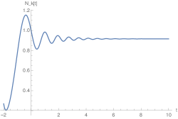
Figure 1: Plot of the pair-creation rate ${\cal N}_{\bf k}(t)$ for the Sauter field with $E_{0}=1$, $\tau=3$, $k_{\parallel}=\omega_{0}=1$.

Only its asymptotic value for $t\to\infty$ is physically meaningful.

3.4 The Gelfand-Dikii equation

To obtain ${\cal N}_{\bf k}(t)$, it is sufficient to know $|\phi_{\bf k}(t)|$. This suggests that it might be more economical to work with $G_{\bf k}(t)\equiv|\phi_{\bf k}(t)|^{2}$, which evolves by a linear third-order differential equation,

$$\dddot{G}_{\bf k}(t)+4\omega^{2}_{\bf k}(t)\dot{G}_{\bf k}(t)+2\bigl{(}\omega_{\bf k}^{2}(t)\bigr{)}^{\cdot}G_{\bf k}(t)=0$$ (14)

with the initial condition

$${\rm lim}_{t\to-\infty}G_{\bf k}(t)=\frac{1}{2\omega_{i}}\,.$$

This is actually the Gelfand-Dikii equation [7]. In terms of $G_{\bf k}$, ${\cal N}_{\bf k}(t)$ is given by

$${\cal N}_{\bf k}(t)=\frac{\ddot{G}_{\bf k}}{4\omega(t)}+\omega(t)G_{\bf k}-\frac{1}{2}\,.$$ (15)

For example, for the Sauter field one has

$$G_{\bf k} = \frac{1-z}{2\omega_{0}\,{\rm e}^{\pi\omega_{0}\tau}}\Bigl{|}\phantom{}_{2}F_{1}(\alpha^{\rm sc},\beta^{\rm sc};\gamma;z)\Bigr{|}^{2}\,.$$ (16)

3.5 Solitonic electric fields

The Gelfand-Dikii equation relates to the resolvent of the mode equation, and through it to the (generalized) KdV equation [7]. In [2, 8] the following infinite family of vector potentials was constructed, related to the solitonic solutions of the KdV equation:

$$qA_{\parallel(p)}(t)\equiv\tilde{k}_{\parallel}-\sqrt{\tilde{k}_{\parallel}^{2}+\frac{p(p+1)\omega_{0}^{2}}{\cosh^{2}(\omega_{0}t)}},\quad p=1,2,\ldots$$ (17)

where $\tilde{k}_{\parallel}$ is a fixed but arbitrary reference momentum. The corresponding squared energies at $k_{\parallel}=\tilde{k}_{\parallel}$ are of Pöschl-Teller type,

$$\omega^{2}_{(p){\bf\tilde{k}}}(t)=\omega_{0}^{2}\Bigl{(}1+\frac{p(p+1)}{\cosh^{2}(\omega_{0}t)}\Bigr{)},\quad p=1,2,\ldots$$

All these “solitonic” electric fields do not produce pairs for $k_{\parallel}=\tilde{k}_{\parallel}$ (although they will generally do so for other values of $k_{\parallel}$). For these solitonic fields, the mode equation can be solved exactly:

$$\phi_{(p)}(t)=\frac{e^{-i\omega_{0}t}}{\sqrt{2\omega_{0}}}\,\Big{(}1+e^{2\omega_{0}t}\Big{)}^{p+1}\,_{2}F_{1}\Big{[}1+p;-i+p+1;1-i;-e^{2\omega_{0}t}\Big{]}\,.$$ (18)

Let us show the resulting ${\cal N}_{\tilde{\bf k}}(t)$ for the simplest case $p=1$:

$${\cal N}_{\bf\tilde{k}}(t) = \frac{4+\rm sech^{4}(\omega_{0}t)(1+2\cosh(2\omega_{0}t))}{8\sqrt{1+2\rm sech^{2}(\omega_{0}t)}}-{1\over 2}\,.$$ (19)

In Fig. 2 we plot this function for $\omega_{0}=1.1$.

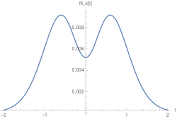
Figure 2: ${\cal N}_{\bf\tilde{k}}(t)$ for the $p=1$ soliton (with $\omega_{0}=1.1$).

Since ${\cal N}_{\bf\tilde{k}}(t)$ vanishes for $t\to\infty$ there is no pair creation at that particular momentum $\bf k=\bf\tilde{k}$. The external field excites the vacuum, but no particles materialize.

4 Generalization to spinor QED

4.1 The mode equation

For spin $\frac{1}{2}$ particles the mode equation becomes [9]

$$\ddot{\psi}_{\bf k}^{(\pm)}(t)+\bigl{[}\omega^{2}_{\bf k}(t)\mp iq\dot{A}_{\parallel}(t)\bigr{]}\psi_{\bf k}^{(\pm)}(t)=0\,,$$ (20)

where the $(\pm)$ denotes the spin. In QFT, this comes from the spin-diagonalized square of the Dirac operator. In [10] it was shown that the constraint equation (5) generalizes to

$$\omega_{\bf k}^{2}|\psi_{\bf k}^{(\pm)}|^{2}+|\dot{\psi}_{\bf k}^{(\pm)}|^{2}\mp i\Pi(\dot{\psi}_{\bf k}^{(\pm)}\psi_{\bf k}^{(\pm)\ast}-\psi_{\bf k}^{(\pm)}\dot{\psi}_{\bf k}^{(\pm)\ast})=\mu^{2}$$ (21)

where $\Pi=k_{\parallel}-qA_{\parallel}(t)$ and that ${\cal N}_{\bf k}(t)$ can, with appropriate initial conditions imposed on $\psi_{\bf k}^{(\pm)}$, be written in terms of the mode solution as

$${\cal N}_{\bf k}(t) = \frac{1}{2\omega_{\bf k}(\omega_{\bf k}-\Pi)}\biggl{[}\omega_{\bf k}^{2}|\psi_{\bf k}^{(\pm)}|^{2}+|\dot{\psi}^{(\pm)}|^{2}\mp i\omega_{\bf k}(\dot{\psi}_{\bf k}^{(\pm)}\psi_{\bf k}^{(\pm)\ast}-\psi_{\bf k}^{(\pm)}\dot{\psi}^{(\pm)\ast})\biggr{]}\,.$$ (22)

Note that ${\cal N}_{\bf k}(t)$ does not depend on the spin orientiation. Combining the last two equations, we can also write

$${\cal N}_{\bf k}(t) = \frac{\mu^{2}}{2\Pi(\omega_{\bf k}-\Pi)}-\frac{\omega_{\bf k}^{2}|\psi_{\bf k}^{(\pm)}|^{2}+|\dot{\psi}_{\bf k}^{(\pm)}|^{2}}{2\omega_{\bf k}\Pi}\,.$$ (23)

4.2 Fermionic Quantum Vlasov Equation

There is also a fermionic generalization of the Quantum Vlasov Equation [5]

$$\dot{\cal N}_{\bf k}(t) = \frac{\mu q\dot{A}_{\parallel}(t)}{2\omega_{\bf k}^{2}(t)}\int_{-\infty}^{t}dt^{\prime}\,\frac{\mu q\dot{A}_{\parallel}(t^{\prime})}{\omega_{\bf k}^{2}(t^{\prime})}\bigl{(}1-2{\cal N}_{\bf k}(t^{\prime})\bigr{)}\cos\Bigl{[}2\int_{t^{\prime}}^{t}dt^{\prime\prime}\omega_{\bf k}(t^{\prime\prime})\Bigr{]}\,.$$ (24)

4.3 Fermionic Gelfand-Dikii equation

Defining $G^{\pm}_{\bf k}\equiv|\psi_{\bf k}^{\pm}|^{2}$ like in the scalar case and combining (20), (21), one arrives at the following generalization of the Gelfand-Dikii equation (14)

$$\dddot{G^{\pm}_{\bf k}}-\frac{E}{\Pi}\ddot{G^{\pm}_{\bf k}}+4\omega_{\bf k}^{2}\dot{G_{\bf k}}+\Bigl{(}2\bigl{(}\omega_{\bf k}^{2}\bigr{)}^{\cdot}-4\frac{E\omega_{\bf k}^{2}}{\Pi}\Bigr{)}G^{\pm}_{\bf k}=-2\mu^{2}\frac{E}{\Pi}\,.$$ (25)

Differentiating the mode equation one can eliminate $|\dot{\psi}^{(\pm)}|^{2}$ and rewrite ${\cal N}_{\bf k}$ in terms of $G_{\bf k}^{\pm}$:

$${\cal N}_{\bf k}=\frac{1}{2}+\frac{\omega_{\bf k}}{\Pi}\Bigl{(}\frac{1}{2}-G_{\bf k}^{\pm}\Bigr{)}-\frac{\ddot{G}_{\bf k}^{\pm}}{4\omega_{\bf k}\Pi}\,.$$ (26)

4.4 Fermions in the solitonic field

A numerical analysis using the Quantum Vlasov Equation (24) suggests that the above solitonic fields (17) are non-pair creating also in the fermionic case, although for different values of the parameter $p$:

$$p={1\over 2}\bigl{(}\pm\sqrt{m^{2}+m+1}-1\bigr{)},\quad m=2,4,6,\ldots$$ (27)

As an example, let us show the result of such a numerical evaluation for the simplest cases $m=2,p={1\over 2}\bigl{(}\pm\sqrt{7}-1\bigr{)}$ (Fig. 3) and $m=4,p={1\over 2}\bigl{(}\pm\sqrt{21}-1\bigr{)}$ (Fig. 4).

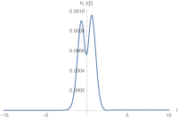
Figure 3: Fermionic ${\cal N}_{\bf\tilde{k}}(t)$ for the $p={1\over 2}\bigl{(}\pm\sqrt{7}-1\bigr{)}$ soliton.

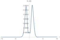
Figure 4: Fermionic ${\cal N}_{\bf\tilde{k}}(t)$ for the $p={1\over 2}\bigl{(}\pm\sqrt{21}-1\bigr{)}$ soliton.

This should be compared to the case $p=1$, which would not pair create in the scalar case but clearly does so here (Fig. 5):

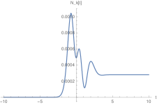
Figure 5: Fermionic ${\cal N}_{\bf\tilde{k}}(t)$ for the $p=1$ soliton.

5 Summary and Outlook

To summarize,

• We have presented an evolution equation for fermions in a purely time-dependent electric field that can be seen as a fermionic generalization of the Gelfand-Dikii equation.

• Solitonic electric fields allow one to tune the pair creation rate to disappear at some prescribed longitudinal momentum for both scalars and spinors, although not for the same field.

• Thus they provide an example of spin selection in the pair creation process, and also a step towards “designer fields”, that is, the construction of fields with a prescribed pair-creation spectrum [11].

• It remains to find an analytic derivation of the “magic numbers” (27).

A more extensive study of fermionic pair creation in solitonic fields is in progress [12].

The work of SPK was supported by the Institute for Basic Science (IBS) under IBS-R012-D1. CS thanks the CIC of UMSNH for financial support.

References

References

[1]
R Dabrowski and G V Dunne, Time dependence of adiabatic particle number, Phys. Rev.
D 94, 065005 (2016), arXiv:1606.00902 [hep-th].
[2]
S P Kim and C Schubert,
Non-adiabatic Quantum Vlasov Equation for Schwinger Pair Production,
Phys .Rev. D 84 125028 (2011), arXiv:1110.0900 [hep-th].
[3]
Y Kluger, J M Eisenberg, B Svetitsky, F Cooper and E Mottola,
Pair production in a strong electric field,
Phys. Rev. Lett. 67 (1991) 2427.
[4]
Y Kluger, J M Eisenberg, B Svetitsky, F Cooper and E Mottola,
Fermion pair production in a strong electric field,
Phys. Rev. D 45 (1992) 4659.
[5]
S Schmidt, D Blaschke, G Röpke, S A Smolyansky, A V Prozorkevich and V D Toneev,
A quantum kinetic equation for particle production in the Schwinger mechanism,
Int. J. Mod. Phys. E 7 (1998) 709, arXiv: hep-ph/9809227.
[6]
F Hebenstreit, R Alkofer and H Gies,
Pair production beyond the Schwinger formula in time-dependent electric fields,
Phys. Rev. D 78, 061701 (2008), arXiv:0807.2785.
[7]
I M Gelfand and A Dikii,
Asymptotic Behavior of the Resolvent of Sturm-Liouville Equations and the Algebra of the Korteweg-De Vries Equations, Russ. Math. Surveys 30, 5 (1975).
[8]
A Huet, S P Kim and C Schubert,
Vlasov equation for Schwinger pair production in a time-dependent electric field,
Phys. Rev. D 90 (2014) 125033, arXiv:1411.3074 [hep-th].
[9]
A B Balantekin, J E Seger and S H Fricke,
Dynamical effects in pair production by electric fields,
Int. J. Mod. Phys. A 6 (1991) 695.
[10]
A M Fedotov, E G Gelfer, K Yu Korolev and S A Smolyansky,
Kinetic equation approach to pair production by a time-dependent electric field,
Phys. Rev. D, 83, 025011 (2011), arXiv:1008.2098 [hep-ph].
[11]
F Hebenstreit,
The inverse problem for Schwinger pair production,
Phys. Lett. B 753 (2016) 336, arXiv:1509.08693 [hep-ph].
[12]
N Ahmadiniaz, A M Fedotov, E G Gelfer, S P Kim and C Schubert,