Voxel Field Fusion for 3D Object Detection

Abstract

In this work, we present a conceptually simple yet effective framework for cross-modality 3D object detection, named voxel field fusion. The proposed approach aims to maintain cross-modality consistency by representing and fusing augmented image features as a ray in the voxel field. To this end, the learnable sampler is first designed to sample vital features from the image plane that are projected to the voxel grid in a point-to-ray manner, which maintains the consistency in feature representation with spatial context. In addition, ray-wise fusion is conducted to fuse features with the supplemental context in the constructed voxel field. We further develop mixed augmentor to align feature-variant transformations, which bridges the modality gap in data augmentation. The proposed framework is demonstrated to achieve consistent gains in various benchmarks and outperforms previous fusion-based methods on KITTI and nuScenes datasets. Code is made available at https://github.com/dvlab-research/VFF.

1 Introduction

Object detection in 3D scenes is regarded as a vital task to provide accurate perception for real-world applications. Over the past decades, research attentions [51, 38, 40, 15, 27] have been dedicated to 3D object detection from raw point clouds. Due to the inherent properties of LiDAR sensors, the captured point clouds are usually sparse and cannot provide sufficient context to distinguish among hard cases in distant or occluded regions, which consequently yields inferior performance in such scenarios. However, in safety-critical applications like autonomous driving, the frequently occurred miss-detection is unacceptable.

To address this issue, previous studies introduce image features in the cross-modality fusion [32, 13, 33]. The main challenge is to maintain the cross-modality consistency in this process that might be damaged in feature representation considering context deficiency and density variance, and data augmentation for cross-modality misalignment. In particular, previous work represents image features in a point-to-point manner in Figure 1(a), which conducts fusion in each single point, constrained by the sparsity of point clouds. In this case, the rich context cues from images cannot be well utilized because adjacency in the image plane cannot be guaranteed in 3D space. Meanwhile, given augmented point clouds, traditional approaches [17, 50] usually keep raw images unchanged and reverse transformations in point clouds for pairwise correspondence. However, because of the flipping and scaling variance in 2D convolutions, the asynchronous augmentation brings cross-modality misalignment and instability.

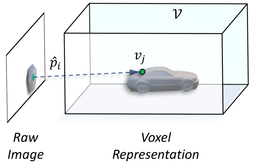
(a) Point-to-point manner

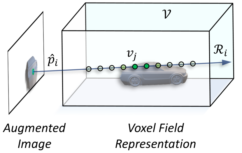
(b) Point-to-ray manner

Figure 1: Compared with previous work [17, 50] in 1(a) that projects feature from raw image to voxel and represents in a point-to-point manner, the proposed method in 1(b) projects feature from augmented image to voxel field and represents in a point-to-ray manner. Dotted and solid arrow denote point- and ray-level projection.

In this paper, we propose a new cross-modality framework, called voxel field fusion (VFF). Mixed augmentation for both modalities is first applied for data-level pre-processing. As briefly illustrated in Figure 1(b), VFF projects augmented image features to the voxel grid and represents it in a point-to-ray manner, called voxel field similar to that in neural rendering [20, 19]. In this way, representations of both modalities are well aligned, and surrounding spatial context is replenished in voxel field. In short, the key idea of VFF is to maintain modality consistency by representing and fusing augmented image feature as a ray in voxel field.

The image-to-voxel dense rendering is usually resource-intensive or requires extra models for depth prediction [25, 47]. To facilitate this process, we draw inspiration from recent advances in neural rendering [20, 19, 48] and propose a learnable sampler and ray-wise fusion for efficient ray construction and cross-modality fusion. In particular, instead of random sampling [20], learnable sampler is designed to select image features for interaction within the activated area with high responses, where features are represented in a point-to-ray manner as aforementioned. Then, ray-wise fusion is conducted in the voxel field according to the predicted score of each voxel along the ray. For the misalignment in augmentation, the mixed augmentor is further proposed to bridge this gap by aligning feature-variant augmentation (flipping and scaling) in image level.

With the above designs, the cross-modality consistency can be maintained from the aspect of feature representation and data augmentation in an end-to-end manner. Generally, the proposed VFF is distinguished from two aspects. First, it projects image features in a point-to-ray manner and represents, as well as fuses them, in the voxel field, which eliminates the modality gap and provides accurate 3D context to detect hard cases. Second, it efficiently samples high-responded features from augmented images, which enables the network to construct each ray on the fly.

The overall framework, called voxel field fusion, can be easily instantiated with various voxel-based backbones for 3D object detection, which is fully elaborated in Section 3. Extensive empirical studies of the designed workflow are conducted in Section 4 to reveal the effect of each component. We further report experimental results on two widely-adopted datasets, namely KITTI [10] and nuScenes [2]. The proposed VFF is proved to achieve consistent increases over various benchmarks and attains significant gain with 2.2% AP over strong baselines on hard cases of KITTI test set. Meanwhile, it surpasses previous fusion-based methods by a large margin and achieves leading performance on nuScenes test set with 68.4% mAP and 72.4% NDS.

2 Related Work

LiDAR-based 3D Detection. Given point clouds as input, traditional LiDAR-based approaches are usually distinguished by their representation for irregular data, e.g., grid and point. Grid-based methods project the point clouds to regular grids and process them by 2D or 3D networks. The methods with 2D networks usually construct 2D bird-view grids [6, 40, 39] or pseudo image [15] and generating 3D bonding boxes on top of it. Meanwhile, the approaches with 3D networks construct 3D voxels from the divided point clouds and predict boxes with detection heads [38, 8, 44]. Point-based methods directly handle raw point cloud with set abstraction [24] and generate 3D proposals on top of it [28, 42, 22, 21]. Given the sparse property of point cloud, the recognition ability is limited due to lack of texture features, especially in real scenes with multiple categories like nuScenes [2] dataset.

Image-based 3D Detection. Previous image-based methods construct the network and extract features from pure monocular or multiple images for 3D box prediction. Given a single image, several monocular-based approaches [1, 31, 35] try to regress and predict 3D boxes directly, while others propose to construct middle-level representation and perform detection on top of it [36, 47]. Because of the depth requirement in 3D detection, previous work also tries to enhance the ability from depth estimation [5, 30, 25]. Another stream for relatively accurate depth is utilizing stereo or multi-view images to construct 3D geometry volume [43, 4, 7] and conduct object detection on top of it. Although depth estimated from multi-view is much better than that from a single image, it still lags behind the accurate point cloud from LiDAR.

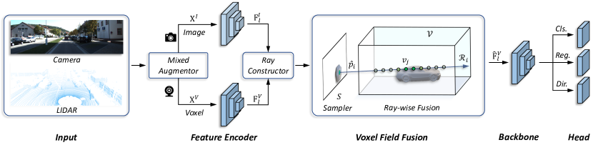
Figure 2: The framework for 3D object detection with voxel field fusion. In particular, inputs with different modalities are firstly processed with the mixed augmentor that is adopted for training only. Then, features of both modalities are respectively extracted in feature encoder, where the correspondence is established in ray constructor. In voxel field fusion, the vital image feature for interaction is selected with the designed sampler. And the ray-wise fusion is then conducted with the high-responded feature along each ray. With the fused and newly generated feature in the voxel field, the following detection backbone and head are applied to predict the final 3D proposals.

Cross-modality Fusion. With inherent limitation of every single modality, there are several methods to combine the strength of image and LiDAR with cross-modality fusion. In particular, point- and proposal-level fusion are introduced to combine features from different modalities. Point-level fusion [17, 13, 33] is usually applied in early stage of the network, while the proposal-based manner [6, 14, 46] is often adopted in the late stage for instance-level fusion. There are also methods that combine these two fusion manners, such as MVX-Net [32]. Compared with proposal-level fusion, the point-level one is a more subtle manner, which is also adopted in our method for deep fusion. Previous point-level fusion approaches [13, 33] usually enhance the point feature from image semantics in a point-to-point manner, ignoring the surrounding context in 3D space. Different from them, the proposed voxel field fusion represents the augmented image feature in a point-to-ray manner in the voxel field, which makes further use of merits from both modalities with sufficient context.

3 Voxel Field Fusion

The overall framework is conceptually simple: mixed augmentor is designed to align data augmentation across modalities; learnable sampler is introduced to efficiently select key features for interaction; and ray-wise fusion is proposed to fuse and combine features along the ray.

3.1 Mixed Augmentor

Given inputs captured from the camera and LiDAR, we first process the data with correspondence, as presented in Figure 2. To this end, a joint strategy, called mixed augmentor, is proposed to handle the aforementioned augmentation misalignment during training from two aspects, namely sample-added and sample-static augmentation.

Sample-added. The sample-added augmentation is defined to increase samples in each scene from the whole database, i.e., GT-sampling [38]. In this case, we supplement the RGB data of sampled 3D objects in a copy-paste manner [9, 49]. That means for each sampled object, we crop data within the projected 2D box and paste it onto the input image, where the crops are reorganized according to the actual depth or the cropping order. In this process, the occluded points covered by near samples are filtered to avoid the cross-modality ambiguity in nuScenes dataset, similar to that of [34].

Sample-static. The sample-static augmentation includes a set of transformations without new sample added, e.g., flipping, rescaling, and rotation. Different from previous work [50, 34], which uses reprojection to find the pairwise correspondence across modalities, we utilize image-level operations for augmentations that affect pretrained 2D convolutions, as summarized in Table 1. Specifically, due to inherent properties like flipping and scaling variance of convolution, the asynchronous augmentation across modalities brings the misalignment. For example, if a flipping operation is applied to point cloud $\mathcal{C}$ but not corresponding images $\mathcal{P}$, the left-right context of point $p_{i}$ projected from point $c_{i}$ would be malposed. We further validate effectiveness of the proposed workflow in Tables 2 and 3.

Table 1: Corresponding operations in the mixed augmentor.

type	Point operation	Image operation
Sample-added	GT-sampling	Copy-paste
Sample-static	Flip	Image-flip
	Rescale	Image-rescale
	Rotate	Reproject

3.2 Voxel Field Construction

With the above designed augmentor, we have input image $\mathbf{X}^{I}\in\mathbb{R}^{H\times W\times 3}$ and voxelized point cloud $\mathbf{X}^{V}\in\mathbb{R}^{X\times Y\times Z\times 4}$, as depicted in Figure 2. The feature encoder with stacked convolutions is applied to extract feature $\mathbf{F}_{l}^{I}$ and $\mathbf{F}_{l}^{V}$ for image and voxel in the $l$-th stage, where $l$ is set to 1 by default and further investigated in Table 7. With the ray constructor, the correspondence between voxel bin $v_{i}$ and image pixel $p_{i}$ is established in voxel field with the given projection matrix $\mathbf{T}_{\mathrm{Voxel\rightarrow{Image}}}$.

Voxel Field. In voxel representation, point clouds of a scene are captured within a voxel space $\mathcal{V}$ that contains several bins. Every single voxel $v$ in it can be represented by the function $\mathcal{F}$, called voxel field. Specifically, for the feature $\mathrm{F}^{V}_{l,v}$ in voxel bin $v$ with coordinates $(x,y,z)$, we have $\mathrm{F}^{V}_{l,v}=\mathcal{F}(x,y,z)$. In the voxel field, the ray $\mathcal{R}_{i}\in\mathcal{V}$ from the point $p_{i}$ through the voxel space $\mathcal{V}$ in a fixed direction is constructed with

$$p_{i}=v_{j}\mathbf{T}^{T}_{\mathrm{Voxel\rightarrow{Image}}},\;\forall v_{j}\in\mathcal{R}_{i}.$$ (1)

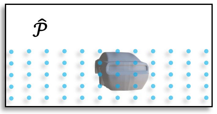
(a) Sample by uniformity

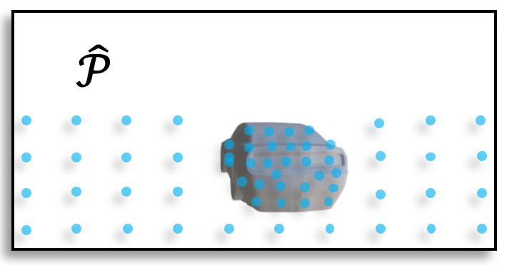
(b) Sample by density

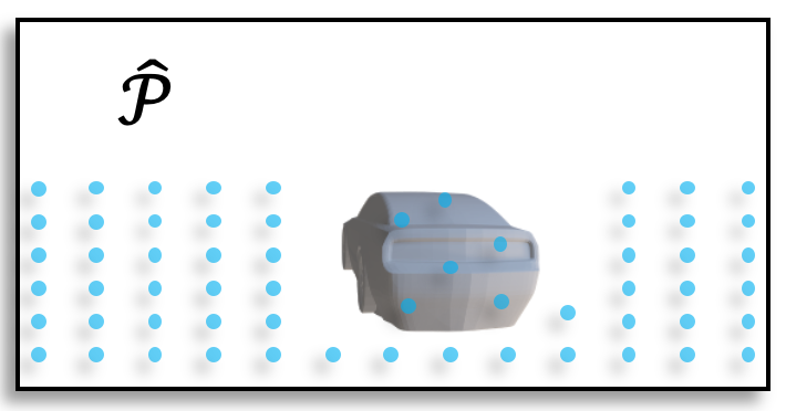
(c) Sample by sparsity

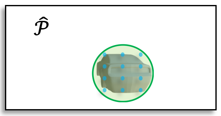
(d) Sample by importance

Figure 3: Toy examples of different sampling methods. The blue points denote the sampled pixels for ray interaction. Compared with heuristic manners, our proposed learnable sampler in 3(d) only considers the important green area with high responses.

This means all voxel bins $v_{j}$ with the same projected point $p_{i}$ are marked to be located in the $i$-th ray set $\mathcal{R}_{i}$. Theoretically, the number of the whole set $\mathcal{R}$ can be up to $W\times H$ if without constraint, which brings huge computational cost that linearly increases with the number of sampled points.

Learnable Sampler. To reduce the computational burden, learnable sampler is proposed to select $n$ points from the image plane for ray interaction, which brings $n$ rays in total. In particular, we first split the image to several non-overlap windows with size $w\times w$ and filter out the empty windows with no projected point $p_{i}$, where $w$ is set to 64 by default. Different from heuristic approaches for sampling, we adopt a learnable strategy to select key features by importance, as illustrated in Figure 3. For heuristic manner, $n$ features from the image plane are randomly sampled according to uniformity, density, and sparsity of projected LiDAR points. Although the heuristic sampling method reduces the cost for ray construction, it still introduces several useless points that could increase computation in this process. To facilitate the efficiency, a learnable sampler $\mathcal{S}$ is further proposed, which only conducts the sampling procedure from the predicted important sub-region with high responses, as depicted in Figure 3(d). Therefore, a set of sampled pixels $\widehat{\mathcal{P}}$ is achieved by

$$\mathcal{S}(\mathcal{P})=\mathcal{U}(\{p_{i}:\mathbbm{1}(\delta(f(\mathrm{F}^{I}_{l,i})))=1\}),$$ (2)

where $f$, $\delta$, and $\mathcal{U}$ denote stacked convolutions, $\mathrm{sigmoid}$ activation, and uniform sampler, respectively. The indicator $\mathbbm{1}$ is set to 1 if the activated response in $p_{i}$ surpasses the threshold 0.5. Considering the importance of foreground instance in 3D detection, here we set the Gaussian region inside each 2D object box to be the positive area for supervision, which is further explained in Section 3.4. In this way, the amount of sampled pixels $\widehat{\mathcal{P}}$, as well as the cost, are further reduced. Meanwhile, the high accuracy is still retained thanks to the proposed learnable sampler, as compared in Table 4.

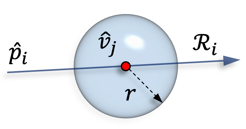
(a) Single fusion with each point

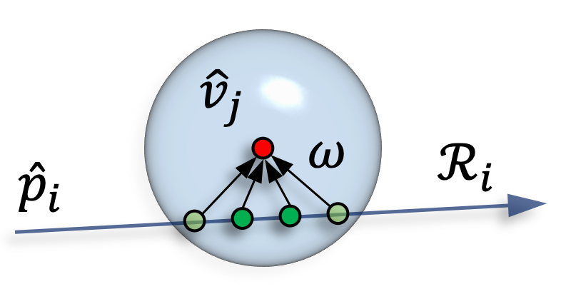
(b) Local fusion with aggregation

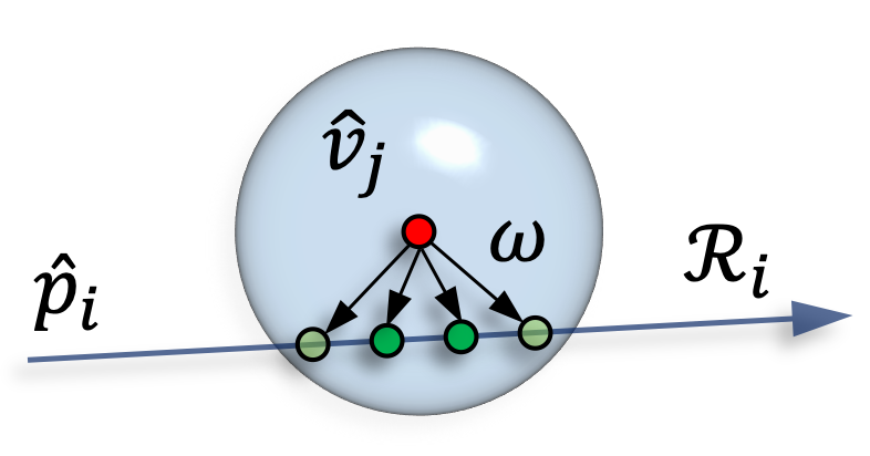
(c) Local fusion with propagation

(d) Ray-wise fusion along the ray

Figure 4: Toy examples of different fusion methods. The red point $\hat{v}_{j}$ denotes the anchor voxel with LiDAR points. Green points in $\mathcal{R}_{i}$ indicate voxel bins $v_{j}$ within the ball with radius $r$. The dotted line in 4(d) represents the assigned existence probability for training.

3.3 Ray-voxel Interaction

Recall from Equation (1), the ray $\mathcal{R}_{i}$ is constructed with the pixel $\hat{p}_{i}\in\widehat{\mathcal{P}}$ from the above designed sampler $\mathcal{S}$. Thus, the cross-modality fusion can be conducted with the ray $\mathcal{R}_{i}$ in the voxel field. Previous research [17, 33, 34] performs fusion with sparse points from LiDAR sensor only, with no consideration of surrounding 3D context, as presented in Figure 4(a). Therefore, a naive solution is to extend the perception region to include points that are located in the nearby region with radius $r$ of the voxel space $\mathcal{V}$, named local fusion. In this section, we first introduce the basic local fusion and then improve over it to formulate the designed ray-wise fusion.

Local Fusion. In this case, two types of local fusion are designed as our benchmark. Given the prior that features along the ray are more likely to be located near LiDAR points and the closer features usually contribute more, local fusion is conducted inside each Gaussian ball and ignores outside features along ray $\mathcal{R}_{i}$. Here, we call the voxels that contains LiDAR points as anchor voxels. The local fusion is divided into aggregation and propagation according to specific operations. The aggregation manner in Figure 4(b) aggregates image features to the anchor voxel $\hat{v}_{j}$ with Gaussian weight $\omega$, while the propagation one in Figure 4(c) propagates features in $\hat{v}_{j}$ to each voxel with weight $\omega$.

Ray-wise Fusion. Although the designed local fusion extends the perception region from a single voxel to near area, it still set a hard boundary in this process. And such an approach cannot fully release the potential of ray-wise representation, especially in most of the voxels without LiDAR points. Thus, besides the anchor voxel $\hat{v}_{j}$, we further extend the operation region to the whole ray, called ray-wise fusion. Compared with single fusion in Figure 4(a), ours is more robust to sensor jitter due to a larger fault-tolerant space brought by Gaussian ball. Different from local fusion, the ray-wise manner in Figure 4(d) takes the above local prior to label assign in the training stage only, as elaborated in Section 3.4. Specifically, given the voxel $v_{j}$ along the ray $\mathcal{R}_{i}$, its probability $\omega_{j}$ is calculated by

$$\omega_{j}=\delta(\left\langle\mathbf{F}^{I}_{l,i},\mathbf{F}^{\prime}_{l,v_{j}}\right\rangle),$$ (3)

where $\delta$ denotes $\mathrm{sigmoid}$ activation, and the voxel feature $\mathbf{F}^{\prime}_{l,v_{j}}=\mathrm{MLP}([x_{j},y_{j},z_{j}])$ is transformed from the coordinate $(x_{j},y_{j},z_{j})$ of $v_{j}$ with multi-layer perceptron. Here, $\omega_{j}$ can be viewed as the response of image feature $\mathbf{F}^{I}_{l,i}$ to the position of $v_{j}$. From another perspective, this operation converts the monocular depth estimation with $\mathbf{F}^{I}_{l,i}$ from a regression problem to classification in a single ray $\mathcal{R}_{i}$. It actually reduces the solution space to a ray. With the predicted score $\omega_{j}$, we conduct the fusion in voxel $v_{j}$ with

$$\widehat{\mathcal{F}}(x_{j},y_{j},z_{j})=\mathcal{F}(x_{j},y_{j},z_{j})+\omega_{j}f([\mathbf{F}^{I}_{l,i},\mathbf{F}^{\prime}_{l,v_{j}}]).$$ (4)

Here, $f$ denotes the convolution. $\widehat{\mathcal{F}}(x_{j},y_{j},z_{j})$ indicates the new generated feature in voxel $v_{j}$. In this process, $\mathcal{F}(x_{j},y_{j},z_{j})$ is set to 0 if the original voxel $v_{j}$ is empty, which can be viewed as completion in empty voxels of $\mathcal{V}$. For network efficiency, only the voxels with top predicted scores $\omega$ are selected for fusion, which accounts for a quarter of original non-empty voxels in total. As presented in Figure 2, the fused feature $\widehat{F}^{V}_{l}$ is obtained for the next stage in the 3D detection backbone and the following detection head. This framework can be instantiated with various voxel-based backbones for experiments in Section 4, e.g., PV-RCNN [27], Voxel R-CNN [8], and CenterPoint [44].

3.4 Optimization Objectives

Recall from Equations (2) and (3), there are two learnable factors required supervision. For learnable sampler $\mathcal{S}$, given the prior that foreground objects are usually more important, we draw Gaussian distribution inside each box with

$$\mathbf{Y}_{l,u,v}=\exp\left(-\frac{(u-\hat{u}_{i})^{2}+(v-\hat{v}_{i})^{2}}{2\sigma_{i}^{2}}\right),$$ (5)

where $(\hat{u}_{i},\hat{v}_{i})$ denotes coordinate of the $i$-th object center, and $\sigma_{i}$ indicates the object size-adaptive standard deviation. For activated probability $\omega_{j}$, the Gaussian-like supervision $\hat{\omega}_{j}$ of voxel $v_{j}$ is formulated as

$$\hat{\omega}_{j}=\exp\left(-\frac{(x-\hat{x}_{j})^{2}+(y-\hat{y}_{j})^{2}+(z-\hat{z}_{j})^{2}}{2\sigma_{j}^{2}}\right),$$ (6)

where $(\hat{x}_{j},\hat{y}_{j},\hat{z}_{j})$ denotes the location of anchor voxel $\hat{v}_{j}$ in Figure 4, and $\sigma_{j}$ indicates the size-adaptive standard deviation. And the voxels with Euclidean distance larger than radius $r$ are assigned as 0, which is investigated in Table 6. In this way, positions of LiDAR points can be utilized to provide supervision for feature selection in the ray. Finally, the objective function of voxel field fusion is defined as

$$\mathcal{L}_{\mathrm{vff}}=\lambda_{\mathrm{s}}\mathrm{BCE}(f(\mathrm{F}^{I}_{l}),\mathbf{Y}_{l})+\lambda_{\mathrm{r}}\sum^{m}\mathrm{FL}(\omega,\hat{\omega})/m,$$ (7)

where $f(\mathrm{F}^{I}_{l})$ represents the convolved feature in Equation (2), and $m$ denotes the size of ray set $\mathcal{R}$. $\mathrm{BCE}$ and $\mathrm{FL}$ indicate the binary cross-entropy loss and focal loss [18], respectively. $\lambda_{\mathrm{s}}$ and $\lambda_{\mathrm{r}}$ denote the balanced loss factor for sampler and ray-wise fusion. The optimization target for the whole network is the summation of raw detection loss $\mathcal{L}_{\mathrm{det}}$ and voxel field fusion loss $\mathcal{L}_{\mathrm{vff}}$.

4 Experiments

In this section, the experimental setup is first introduced. Then, we give the analysis of each component on KITTI val set with PV-RCNN [27] as the backbone. Comparisons with previous work on nuScenes [2] and KITTI [10] datasets are reported in the end.

4.1 Experimental Setup

Dataset. KITTI dataset [10] is a widely-adopted multi-modality benchmark for 3D object detection, which provides synced LiDAR points and front-view camera images. It contains 7,481 samples for training and 7,518 samples for testing, where the training samples are usually split to train set with 3,712 samples and val set with 3,769 samples. nuScenes dataset [2] is a large-scale benchmark for autonomous driving with 1,000 scenes, which are divided into 700, 150, 150 scenes in the train set, val set, and test set, respectively. Here, we use the synced data with 10 object categories that are collected from a 32-beam LiDAR and six cameras in a 360-degree field of view.

Implementation Details. In this work, three different backbones are adopted to validate the proposed framework, i.e., PV-RCNN [27] and Voxel R-CNN [8] on KITTI dataset, and CenterPoint [44] on nuScenes dataset. We follow corresponding architecture and training settings in each network. In the proposed VFF, three convolutions and MLPs are applied to the learnable sampler in Equation (2) and feature transformation in Equation (3), where individual MLP is used for each camera view. For optimization, $\lambda_{\mathrm{s}}$ and $\lambda_{\mathrm{r}}$ in Equation (7) is set to 2 and 5 in all our experiments. Besides the non-empty voxels, we select features along each ray with probability $\omega$ bigger than 0.05 in the inference stage.

4.2 Component-wise Analysis

Aligned Augmentation. As elaborated in Section 3.1, aligned data plays a vital role in cross-modality consistency. In Table 2, we compare the joint strategy for the sample-static augmentation listed in Table 1, where PV-RCNN and basic single fusion are adopted. As compared in Table 2, the designed image-level transformation contributes significantly to feature-variant augmentations, namely Flip and Rescale. If flip augmentation is adopted only, the performance gain is up to 1.65% AP on moderate cases.

Table 2: Comparisons on different augmentations on the KITTI val set. aug type and align type denote the adopted sample-static augmentation and type of cross-modality alignment, respectively.

aug type	align type		AP3D@Car-R40 (IoU=0.7)
			Easy	Moderate	Hard
None	–		88.69	81.82	79.91
+ Flip	reproject		89.26	82.50	82.27
	ours		91.34	84.15	82.48
+ Rescale	reproject		91.78	84.25	82.58
	ours		91.68	84.53	82.59
+ Rotate	reproject		91.30	84.45	82.64
	ours		91.43	84.57	82.61

Table 3: Comparisons on different strategies in mixed augmentor on the KITTI val set. strategy and fusion denote the strategy in mixed augmentor and the usage of voxel field fusion, respectively.

strategy	fusion		AP3D@Car-R40 (IoU=0.7)
			Easy	Moderate	Hard
Original	✗		86.40	75.47	71.32
	✓		87.08	76.25	72.03
+ Added	✗		87.77	79.19	76.71
	✓		89.56	82.53	80.00
+ Static	✗		91.53	84.36	82.29
	✓		92.31	85.51	82.92

Table 4: Comparisons on different sampling types on the KITTI val set. sample type and learn denote the adopted sampler and learnable manner for feature selection in Section 3.2, respectively.

sample type	learn		AP3D@Car-R40 (IoU=0.7)
			Easy	Moderate	Hard
Uniformity	✗		88.69	81.90	79.82
Sparsity	✗		89.09	81.68	79.85
Density	✗		88.72	82.01	81.42
Importance	✓		89.11	82.10	79.98

Mixed Augmentor. The proposed mixed augmentor in Section 3.1 maintains consistency in augmentation from sample-added and sample-static strategies. Here, we investigate the augmentor with VFF in Table 3. In the mixed augmentor, sample-added strategy yields notable gain with 6.28% AP. With the sample-static manner, the network with VFF is further improved to 85.51% AP on moderate cases. For clear comparisons, the following ablation studies are conducted with sample-added strategy only by default.

Learnable Sampler. To facilitate voxel field construction, learnable sampler is proposed in Section 3.2. In Table 4, different sampling methods are compared, which are divided into heuristic and learnable sets. As presented in Figure 3, the heuristic sampler contains the type of uniformity, sparsity, and density. And the network with heuristic sampler achieves peak performance with 82.01%AP when sampling based on density. As for the learnable sampler, the proposed sampling with importance in Figure 3(d) attains a superior result than the heuristic one with 82.10% AP.

Table 5: Comparisons on different fusion strategies on the KITTI val set. range and operation denote the fusion range and specific operation, respectively. Single fusion is a subset of the others.

range	operation		AP3D@Car-R40 (IoU=0.7)
			Easy	Moderate	Hard
Single	–		88.69	81.82	79.91
Local	aggregate		89.00	82.12	81.52
	propagate		89.16	82.07	81.17
Ray-wise	generate		89.56	82.53	80.00

Table 6: Comparisons on different types of supervision on the KITTI val set. radius and gaussian denote the adopted radius $r$ and the usage of Gaussian distribution in Section 3.3, respectively.

radius	gaussian		AP3D@Car-R40 (IoU=0.7)
			Easy	Moderate	Hard
0	✗		89.11	82.10	79.98
1	✓		89.56	82.53	80.00
2	✓		88.33	81.75	79.54

Table 7: Comparisons on different fusion positions on the KITTI val set. stage and fusion denote the specific fusion stage in the network and the usage of voxel field fusion, respectively.

stage	fusion		AP3D@Car-R40 (IoU=0.7)
			Easy	Moderate	Hard
–	✗		87.77	79.19	76.71
Stage-1	✓		89.56	82.53	80.00
Stage-2	✓		89.12	80.43	79.70
Stage-3	✓		89.64	80.27	77.93
Stage-4	✓		88.69	80.22	78.10

Table 8: Comparisons on different methods with a single model on the KITTI val set. * denotes our result from official source code.

method		AP3D@Car-R40 (IoU=0.7)				AP3D@Car-R11 (IoU=0.7)				APBEV@Car-R40 (IoU=0.7)
		Easy	Moderate	Hard		Easy	Moderate	Hard		Easy	Moderate	Hard
LiDAR-based
SECOND [38]		–	–	–		87.43	76.48	69.10		–	–	–
PointRCNN [28]		–	–	–		88.88	78.63	77.38		–	–	–
STD [42]		–	–	–		89.70	79.80	79.30		–	–	–
PV-RCNN [27]		92.57	84.83	82.69		89.35	83.69	78.70		95.76	91.11	88.93
Voxel R-CNN [8]		92.38	85.29	82.86		89.41	84.52	78.93		95.52	91.25	88.99
LiDAR+RGB
UberATG-MMF [16]		–	–	–		88.40	77.43	70.22		–	–	–
3D-CVF [46]		89.67	79.88	78.47		–	–	–		–	–	–
EPNet [13]		92.28	82.59	80.14		–	–	–		95.51	88.76	88.36
PV-RCNN*		91.53	84.36	82.29		88.95	83.51	78.72		92.82	90.43	88.41
+ VFF		92.31	85.51	82.92		89.45	84.21	79.13		95.43	91.40	90.66
Voxel R-CNN*		92.27	84.88	82.50		89.46	83.61	78.80		95.51	91.13	88.85
+ VFF		92.47	85.65	83.38		89.51	84.76	79.21		95.65	91.75	91.39

Table 9: Comparisons on cross-modality fusion of different categories on the KITTI val set. We report results of car, pedestrian, and cyclist with IoU=0.7, 0.5, and 0.5, respectively.

category	fusion		AP3D-R40
			Easy	Moderate	Hard
Car	✗		91.53	84.36	82.29
	✓		92.31	85.51	82.92
Pedestrian	✗		66.04	59.19	54.15
	✓		73.26	65.11	60.03
Cyclist	✗		91.31	72.18	67.60
	✓		89.40	73.12	69.86

Table 10: Comparisons on different types of pretrained 2D backbone on the KITTI val set. model denotes the adopted pretrained model in feature encoder with corresponding task.

model	AP3D@Car-R40 (IoU=0.7)
	Easy	Moderate	Hard
Cls: ResNet [12]	91.96	85.33	84.24
Det: Faster R-CNN [26]	91.98	85.11	82.52
Seg: DeepLabV3 [3]	92.31	85.51	82.92

Table 11: Comparisons on cross-modality fusion of different data on the KITTI val set. beam num and fusion denote LiDAR beam number and the usage of voxel field fusion, respectively.

beam num	fusion		AP3D@Car-R40 (IoU=0.7)
			Easy	Moderate	Hard
Beam-64	✗		91.53	84.36	82.29
	✓		92.31	85.51	82.92
Beam-32	✗		91.14	79.51	76.54
	✓		92.20	82.36	79.81

Ray-voxel Interaction. The interaction between ray and voxel is a core operation of the proposed framework in Section 3.3. Here, we compare different fusion methods presented in Figure 4. As shown in Table 5, the performance improves with fusion range increases from a single point to the whole ray. Compared with single fusion and local fusion, the ray-wise strategy surpasses them with a significant gap, which proves the effectiveness of ray-wise fusion.

Ray-wise Supervision. Considering noise from sensor jitter or other issues, the Gaussian-like assignment is proposed to provide supervision in Figure 4(d) and Equation (6). Different supervision strategies are compared in Table 6. It is clear that the Gaussian distribution with radius 1 results in the best performance 82.53% AP. And extra region provides wrong guidance to the ray that goes through each Gaussian ball, which harms feature localization in each ray.

Fusion Stage. We further investigate the fusion stage of the proposed VFF in Table 7. Compared with the baseline, the designed fusion yields superior performance in each stage. The early-stage fusion contributes more, which surpasses the baseline with 3.34% AP. Meanwhile, fusion in the later stage brings less gain, which could be attributed to the low resolution for key feature selection and insufficient fusion.

Different Categories. The ray-wise representation of image features in VFF introduces sufficient context for ambiguous examples. In Table 9, we report comparisons with VFF on various categories. It is clear that the performance of each class has been improved especially for pedestrian, which is up to nearly 6% AP on cases of all difficulties.

Pretrained Network. In Table 10, we analyze the pretrained 2D backbone, which provides the feature $\mathbf{F}^{I}_{l}$ in the feature encoder of Figure 2. Here, we adopt all the augmentations and ResNet-50 based models for different tasks in Table 10, i.e., classification, detection, and semantic segmentation. Compared with other tasks, the network [3] provides better features if pretrained with semantic setting.

Table 12: Comparisons on different methods with single model on the nuScenes test set.

method	mAP	NDS	Car	Truck	Bus	Trailer	C.V.	Ped.	Motor.	Bicycle	T.C.	Barrier
LiDAR-based
PointPillars [15]	30.5	45.3	68.4	23.0	28.2	23.4	4.1	59.7	27.4	1.1	30.8	38.9
3DSSD [41]	42.6	56.4	81.2	47.2	61.4	30.5	12.6	70.2	36.0	8.6	31.1	47.9
CBGS [52]	52.8	63.3	81.1	48.5	54.9	42.9	10.5	80.1	51.5	22.3	70.9	65.7
CenterPoint [44]	60.3	67.3	85.2	53.5	63.6	56.0	20.0	84.6	59.5	30.7	78.4	71.1
LiDAR+RGB
PointPainting [33]	46.4	58.1	77.9	35.8	36.2	37.3	15.8	73.3	41.5	24.1	62.4	60.2
FusionPainting [37]	66.3	70.4	86.3	58.5	66.8	59.4	27.7	87.5	71.2	51.7	84.2	70.2
MVP [45]	66.4	70.5	86.8	58.5	67.4	57.3	26.1	89.1	70.0	49.3	85.0	74.8
PointAugmenting [34]	66.8	71.0	87.5	57.3	65.2	60.7	28.0	87.9	74.3	50.9	83.6	72.6
VFF + CenterPoint	68.4	72.4	86.8	58.1	70.2	61.0	32.1	87.1	78.5	52.9	83.8	73.9

Table 13: Comparisons on different methods on KITTI test set.

method		AP3D@Car-R40 (IoU=0.7)
		Easy	Moderate	Hard
LiDAR-based
PointPillars [15]		82.58	74.31	68.99
PointRCNN [28]		86.96	75.64	70.70
Part-$A^{2}$ [29]		87.81	78.49	73.51
STD [42]		87.95	79.71	75.09
SA-SSD [11]		88.75	79.79	74.16
PV-RCNN [27]		90.25	81.43	76.82
Voxel R-CNN [8]		90.90	81.62	77.06
LiDAR+RGB
MV3D [6]		74.97	63.63	54.00
F-PointNet [23]		82.19	69.79	60.59
AVOD [14]		83.07	71.76	65.73
UberATG-MMF [16]		88.40	77.43	70.22
EPNet [13]		89.81	79.28	74.59
3D-CVF [46]		89.20	80.05	73.11
VFF + PV-RCNN		89.58	81.97	79.17
VFF + Voxel R-CNN		89.50	82.09	79.29

Sparse LiDAR. To verify the effectiveness of VFF with different LiDAR sparsity, we downsample the LiDAR points on the KITTI dataset to 32-beam following [47]. As presented in Table 11, the proposed VFF achieves significant gain with 2.85% AP over the baseline. For hard cases, the gap is enlarged to 3.27% AP. It could attribute to the replenishment of empty voxels that lack LiDAR points.

4.3 Main Results

nuScenes. We further report results on the large scale nuScenes test set. As shown in Table 15, the proposed method surpasses all previous approaches with 68.4% mAP and 72.4% NDS. Compared with our strong backbone CenterPoint [44], the performance gain brought by VFF is up to 8.1% mAP and 5.1% NDS. As for ambiguous classes like motorcycle and bicycle, the gain is even up to 19% AP.

KITTI. In Table 8, we carry out experiments on KITTI val set. Compared with the baseline, our proposed VFF achieves consistent gain on various evaluation metrics and attains 85.51% and 85.65% AP with PV-RCNN [27] and Voxel R-CNN [8], respectively. The result on KITTI test set is reported on Table 13. Compared with previous fusion-based methods, the proposed VFF pushes the top performance to 81.97% AP and 82.09% AP with PV-RCNN and Voxel R-CNN as the backbone, respectively. Thanks to the designed fusion manner, our method outperforms all previous models on hard cases with 79.29% AP, which attains 2.2% AP improvement over the baseline.

5 Conclusion

We have presented the voxel field fusion, a conceptually simple yet effective framework for cross-modality fusion in 3D object detection. The key difference from prior works lies in that we maintain modality consistency by representing and fusing augmented image features as a ray in the voxel field. In particular, inconsistency in feature representation for multi-modalities is eliminated with learnable sampler and ray-wise fusion. Meanwhile, the mixed augmentor is developed to bridge the gap in cross-modality data augmentation. Experiments on KITTI and nuScenes dataset prove the effectiveness of the proposed framework, which achieves consistent gains in various benchmarks and surpasses previous fusion-based models on both datasets.

6 Acknowledgments

We thank Yilun Chen and Tao Hu for their suggestions. This work is supported by The National Key Research and Development Program of China (No. 2017YFA0700800) and Beijing Academy of Artificial Intelligence (BAAI).

Appendix A Experimental Details

Here, we provide more details in the network architecture and training process of the proposed voxel field fusion.

A.1 Network Architecture

Voxel-based Network. In our experiments, the voxel-based network is adopted as the main framework. In particular, we conduct experiments with different networks on corresponding official implementations, i.e., OpenPCDet for PV-RCNN [27] and Voxel R-CNN [8] on the KITTI [10] dataset, and CenterPoint [44] on the nuScenes [2] dataset. And all the settings are kept identical with the original version, except the experiment with beam-32 LiDAR in Table 11, where the number of voxels is reduced to a half.

Image-based Network. The image-based feature encoder is required in the proposed cross-modality fusion, as depicted in Figure 2. For different models in Table 10, only the basic backbone with ResNet-50 is utilized to provide the feature $\mathbf{F}^{I}_{l}$ in the $l$-th stage. Feature encoders for different modalities in Figure 2 are aligned to have a same block depth. Specifically, in the $l$-th stage of the voxel-based network, we first extract the image feature $\mathbf{F}^{I}_{l}$ from the corresponding $l$-th stage of the pretrained model. Then, the feature $\mathbf{F}^{I}_{l}$ is upsampled to have the same stride of that in voxel feature $\mathbf{F}^{V}_{l}$. Therefore, the cross-modality correspondence can be established in the calibrator of Figure 2.

A.2 Training Process

Detailed Settings. As declared before, for the voxel-based network, we follow all settings in the corresponding framework for fair comparisons. Meanwhile, for the image-based network, we detach the grad from the original backbone and update the parameters of adopted blocks using grad from the voxel-based network only. Due to the variance in datasets, different strategies are adopted for network evaluation. In particular, for the KITTI dataset, we follow common practice in [27,8] and report the top performance of car in last 10 epoches for stable comparisons. For the nuScenes dataset, we report the performance of the final optimized model.

Augmentation. In Section 3.1 of the main paper, image-level transformation is proposed in the sample-static strategy of mixed augmentor. Specifically, for image-level operations in Table 1, we first randomly sample 100 projected points from LiDAR and calculate the affine matrix according to selected transformed points. Then, the image-level augmentation is conducted with the affine matrix. Due to the asymmetrical arrangement of six cameras, image-level augmentations in the nuScene dataset can not be well-aligned. Thus, we apply the image-level augmentations on KITTI and keep the reproject manner on nuScenes dataset.

Table 14: Comparisons with different methods for context enlargement on the KITTI val set. operation and 3D denote the operation to enlarge context and the action in 3D voxel space, respectively.

operation	3D		AP3D@Car-R40 (IoU=0.7)
			Easy	Moderate	Hard
Single	✗		91.43	84.57	82.61
Conv	✗		91.93	84.89	82.69
Deform Conv	✗		92.10	84.91	82.98
Attention	✗		91.29	83.78	82.14
Ray-wise	✓		92.31	85.51	82.92

Appendix B Additional Analysis

Captured Context. In Table 14, we investigate approaches to enlarge the captured context. In particular, compared with single fusion in Figure 4a, two types of methods are compared by capturing rich context in the image plane and 3D voxel space. As illustrated in Table 14, additional operations in the image plane bring limited gain. It is attributed to the damage of adjacency relation in the voxel space, as analysed before. And the ray-wise manner achieves noticeable gains with geometry priors for context casting.

Table 15: Comparisons with different numbers of views on the nuScenes val set. * denotes our result from the official source code.

method	mAP	NDS	Car	Truck	Bus	Trailer	C.V.	Ped.	Motor.	Bicycle	T.C.	Barrrier
CenterPoint*	58.9	66.4	85.4	56.9	69.7	36.0	17.5	85.1	59.7	40.8	70.0	67.6
+ VFF-1 view	58.6	66.1	85.4	57.1	70.7	37.2	17.1	84.5	59.9	38.8	69.0	66.4
+ VFF-3 view	60.1	67.1	85.8	59.1	71.4	39.4	18.3	85.7	62.5	40.8	72.0	66.1
+ VFF-6 view	63.4	68.7	86.4	60.1	71.7	38.8	23.8	86.2	71.5	52.2	75.8	68.0
+ Fade [34]	65.2	70.1	87.2	60.9	72.1	39.2	25.0	87.0	73.2	61.1	77.0	69.7
+ Flip Test	66.3	71.2	87.6	62.7	72.8	40.5	26.5	87.5	75.0	62.7	77.8	70.0

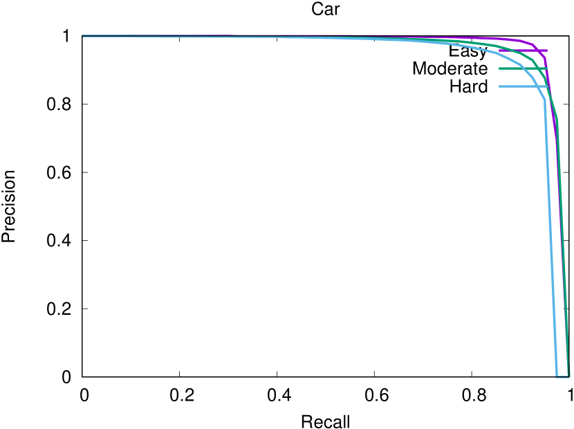
(a) Car: Detection

(b) Car: Orientation

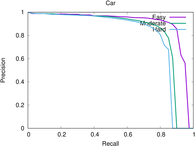
(c) Car: 3D Detection

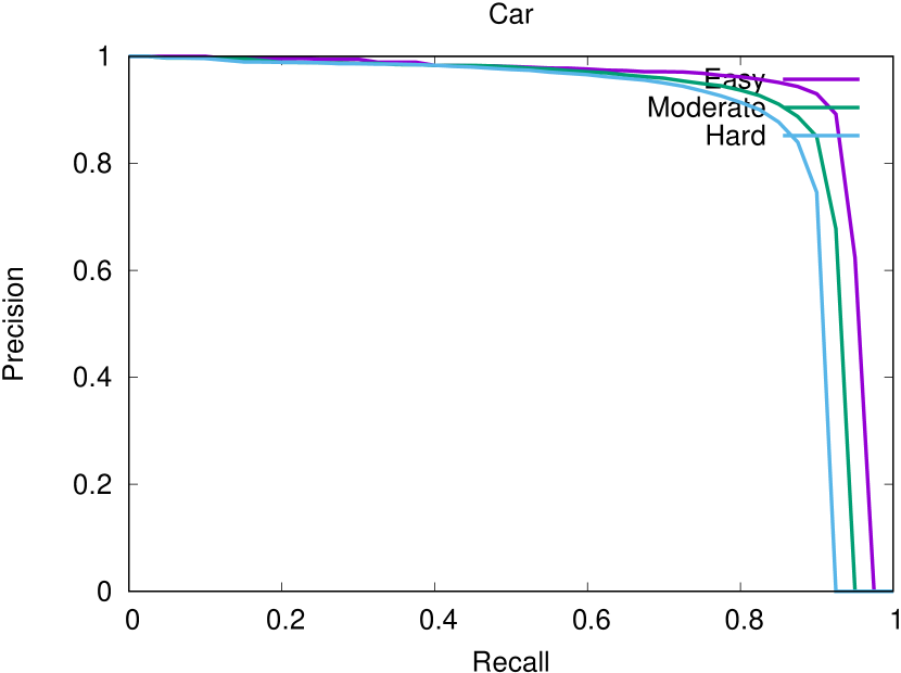
(d) Car: Bird’s Eye View

Figure 5: Precision-Recall curves of Voxel R-CNN with the proposed voxel field fusion on the KITTI test set.

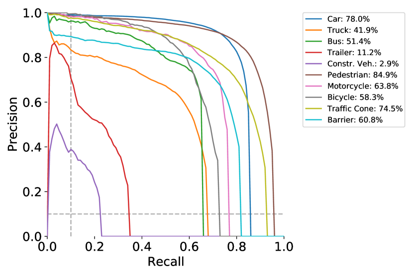
(a) Threshold: 0.5m

(b) Threshold: 1.0m

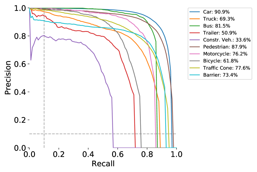
(c) Threshold: 2.0m

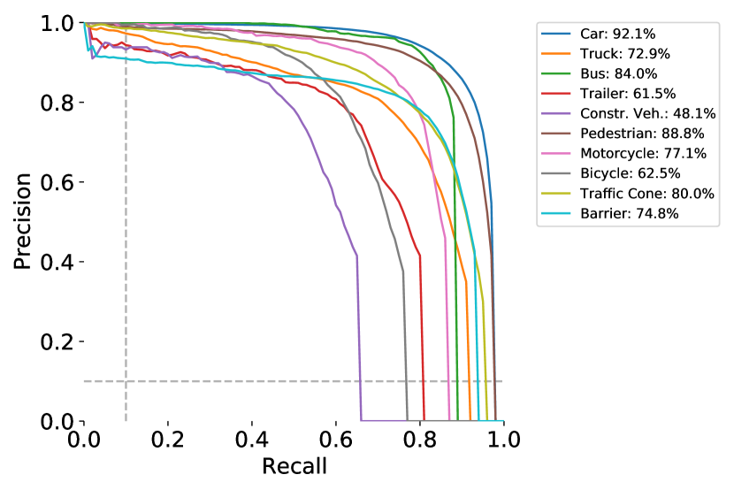
(d) Threshold: 4.0m

Figure 6: Precision-Recall curves of CenterPoint with the proposed voxel field fusion on the nuScenes val set.

Figure 7: Examples of the output predictions in different scenes on the nuScenes val set.

Number of Views. In Table 15, we conduct experiments with different numbers of views on nuScenes dataset. It is clear that the performance increases significantly with more views added, and attains top performance with 4.5% AP gain over the strong baseline. An interesting finding is that fusion with one view brings little performance drop. It could be attributed to the non-uniform distribution brought by part of image features in each scene. With more training and testing strategies, the model achieves 66.3% mAP and 71.2% NDS on nuScenes val set. Here, Fade strategy [34] denotes training without GT-Sampling in last 5 epoch.

Detailed Results. In Figure 5, we draw precision-recall (PR) curves of car on KITTI test set. The proposed method achieves satisfactory results on various metrics. Meanwhile, we present PR curves with various thresholds on nuScenes val set. It is obvious that the network attains good results for common vehicles like car and bus, while achieves inferior results in uncommon objects like construct vehicle.

Predictions on nuScenes. As for large-scale scenes in the nuScenes [2] dataset, we present the predictions in Figure 7. It is clear that the proposed framework predicts satisfactory results with images from the 360-degree field of view.

Appendix C Qualitative Results

In this section, qualitative studies of key components in the proposed framework are conducted with analysis.

Mixed Augmentor. In Figure 8, we present images with randomly adopted operations in the mixed augmentor. It is clear that the cross-modality correspondence is well aligned in various scenes with designed image-level augmentations.

Voxel Field Fusion. We further visualize predictions of each component, as shown in Figure 9. Given inputs with different modalities in various scenes, learnable sampler in Figure 9(a) and ray-wise fusion in Figure 9(b) works well.

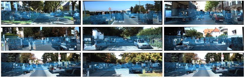
Figure 8: Examples of the proposed mixed augmentor on KITTI val set. The blue points indicate the projected LiDAR in the image plane.

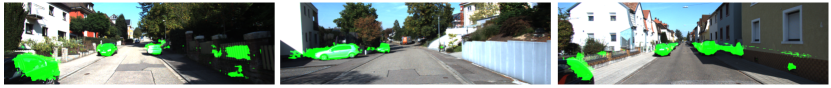
(a) Examples of important areas with the proposed learnable sampler. The green region in each figure indicates activated part with high responses.

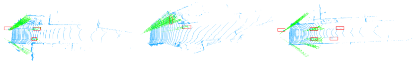
(b) Examples of selected points for ray-wise fusion in BEV. The green points locate newly generated features, and red boxes indicate annotated objects.

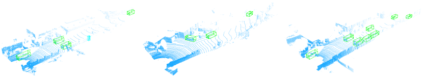
(c) Examples of the output predictions in different scenes. The green and light blue boxes represent the predicted cars and pedestrians.

Figure 9: Examples of key components in the voxel field fusion on KITTI val set. The figures in each column belong to the same scene.

References

- [1] Garrick Brazil and Xiaoming Liu. M3d-rpn: Monocular 3d region proposal network for object detection. In ICCV, 2019.
- [2] Holger Caesar, Varun Bankiti, Alex H Lang, Sourabh Vora, Venice Erin Liong, Qiang Xu, Anush Krishnan, Yu Pan, Giancarlo Baldan, and Oscar Beijbom. nuscenes: A multimodal dataset for autonomous driving. In CVPR, 2020.
- [3] Liang-Chieh Chen, George Papandreou, Florian Schroff, and Hartwig Adam. Rethinking atrous convolution for semantic image segmentation. arXiv:1706.05587, 2017.
- [4] Rui Chen, Songfang Han, Jing Xu, and Hao Su. Point-based multi-view stereo network. In ICCV, 2019.
- [5] Xiaozhi Chen, Kaustav Kundu, Yukun Zhu, Andrew G Berneshawi, Huimin Ma, Sanja Fidler, and Raquel Urtasun. 3d object proposals for accurate object class detection. In NeurIPS, 2015.
- [6] Xiaozhi Chen, Huimin Ma, Ji Wan, Bo Li, and Tian Xia. Multi-view 3d object detection network for autonomous driving. In CVPR, 2017.
- [7] Yilun Chen, Shu Liu, Xiaoyong Shen, and Jiaya Jia. Dsgn: Deep stereo geometry network for 3d object detection. In CVPR, 2020.
- [8] Jiajun Deng, Shaoshuai Shi, Peiwei Li, Wengang Zhou, Yanyong Zhang, and Houqiang Li. Voxel r-cnn: Towards high performance voxel-based 3d object detection. In AAAI, 2021.
- [9] Nikita Dvornik, Julien Mairal, and Cordelia Schmid. Modeling visual context is key to augmenting object detection datasets. In ECCV, 2018.
- [10] Andreas Geiger, Philip Lenz, and Raquel Urtasun. Are we ready for autonomous driving? the kitti vision benchmark suite. In CVPR, 2012.
- [11] Chenhang He, Hui Zeng, Jianqiang Huang, Xian-Sheng Hua, and Lei Zhang. Structure aware single-stage 3d object detection from point cloud. In CVPR, 2020.
- [12] Kaiming He, Xiangyu Zhang, Shaoqing Ren, and Jian Sun. Deep residual learning for image recognition. In CVPR, 2016.
- [13] Tengteng Huang, Zhe Liu, Xiwu Chen, and Xiang Bai. Epnet: Enhancing point features with image semantics for 3d object detection. In ECCV, 2020.
- [14] Jason Ku, Melissa Mozifian, Jungwook Lee, Ali Harakeh, and Steven L Waslander. Joint 3d proposal generation and object detection from view aggregation. In IROS, 2018.
- [15] Alex H Lang, Sourabh Vora, Holger Caesar, Lubing Zhou, Jiong Yang, and Oscar Beijbom. Pointpillars: Fast encoders for object detection from point clouds. In CVPR, 2019.
- [16] Ming Liang, Bin Yang, Yun Chen, Rui Hu, and Raquel Urtasun. Multi-task multi-sensor fusion for 3d object detection. In CVPR, 2019.
- [17] Ming Liang, Bin Yang, Shenlong Wang, and Raquel Urtasun. Deep continuous fusion for multi-sensor 3d object detection. In ECCV, 2018.
- [18] Tsung-Yi Lin, Priya Goyal, Ross Girshick, Kaiming He, and Piotr Dollár. Focal loss for dense object detection. In ICCV, 2017.
- [19] Lingjie Liu, Jiatao Gu, Kyaw Zaw Lin, Tat-Seng Chua, and Christian Theobalt. Neural sparse voxel fields. In NeurIPS, 2020.
- [20] Ben Mildenhall, Pratul P Srinivasan, Matthew Tancik, Jonathan T Barron, Ravi Ramamoorthi, and Ren Ng. Nerf: Representing scenes as neural radiance fields for view synthesis. In ECCV, 2020.
- [21] Charles R Qi, Xinlei Chen, Or Litany, and Leonidas J Guibas. Imvotenet: Boosting 3d object detection in point clouds with image votes. In CVPR, 2020.
- [22] Charles R Qi, Or Litany, Kaiming He, and Leonidas J Guibas. Deep hough voting for 3d object detection in point clouds. In ICCV, 2019.
- [23] Charles R Qi, Wei Liu, Chenxia Wu, Hao Su, and Leonidas J Guibas. Frustum pointnets for 3d object detection from rgb-d data. In CVPR, 2018.
- [24] Charles R Qi, Li Yi, Hao Su, and Leonidas J Guibas. Pointnet++: Deep hierarchical feature learning on point sets in a metric space. In NeurIPS, 2017.
- [25] Cody Reading, Ali Harakeh, Julia Chae, and Steven L Waslander. Categorical depth distribution network for monocular 3d object detection. In CVPR, 2021.
- [26] Shaoqing Ren, Kaiming He, Ross Girshick, and Jian Sun. Faster r-cnn: towards real-time object detection with region proposal networks. TPAMI, 2016.
- [27] Shaoshuai Shi, Chaoxu Guo, Li Jiang, Zhe Wang, Jianping Shi, Xiaogang Wang, and Hongsheng Li. Pv-rcnn: Point-voxel feature set abstraction for 3d object detection. In CVPR, 2020.
- [28] Shaoshuai Shi, Xiaogang Wang, and Hongsheng Li. Pointrcnn: 3d object proposal generation and detection from point cloud. In CVPR, 2019.
- [29] Shaoshuai Shi, Zhe Wang, Jianping Shi, Xiaogang Wang, and Hongsheng Li. From points to parts: 3d object detection from point cloud with part-aware and part-aggregation network. TPAMI, 2020.
- [30] Xuepeng Shi, Zhixiang Chen, and Tae-Kyun Kim. Distance-normalized unified representation for monocular 3d object detection. In ECCV, 2020.
- [31] Andrea Simonelli, Samuel Rota Bulo, Lorenzo Porzi, Manuel López-Antequera, and Peter Kontschieder. Disentangling monocular 3d object detection. In ICCV, 2019.
- [32] Vishwanath A Sindagi, Yin Zhou, and Oncel Tuzel. Mvx-net: Multimodal voxelnet for 3d object detection. In ICRA, 2019.
- [33] Sourabh Vora, Alex H Lang, Bassam Helou, and Oscar Beijbom. Pointpainting: Sequential fusion for 3d object detection. In CVPR, 2020.
- [34] Chunwei Wang, Chao Ma, Ming Zhu, and Xiaokang Yang. Pointaugmenting: Cross-modal augmentation for 3d object detection. In CVPR, 2021.
- [35] Tai Wang, Xinge Zhu, Jiangmiao Pang, and Dahua Lin. Fcos3d: Fully convolutional one-stage monocular 3d object detection. arXiv:2104.10956, 2021.
- [36] Yan Wang, Wei-Lun Chao, Divyansh Garg, Bharath Hariharan, Mark Campbell, and Kilian Q Weinberger. Pseudo-lidar from visual depth estimation: Bridging the gap in 3d object detection for autonomous driving. In CVPR, 2019.
- [37] Shaoqing Xu, Dingfu Zhou, Jin Fang, Junbo Yin, Zhou Bin, and Liangjun Zhang. Fusionpainting: Multimodal fusion with adaptive attention for 3d object detection. In ITSC, 2021.
- [38] Yan Yan, Yuxing Mao, and Bo Li. Second: Sparsely embedded convolutional detection. Sensors, 2018.
- [39] Bin Yang, Ming Liang, and Raquel Urtasun. Hdnet: Exploiting hd maps for 3d object detection. In CoRL, 2018.
- [40] Bin Yang, Wenjie Luo, and Raquel Urtasun. Pixor: Real-time 3d object detection from point clouds. In CVPR, 2018.
- [41] Zetong Yang, Yanan Sun, Shu Liu, and Jiaya Jia. 3dssd: Point-based 3d single stage object detector. In CVPR, 2020.
- [42] Zetong Yang, Yanan Sun, Shu Liu, Xiaoyong Shen, and Jiaya Jia. Std: Sparse-to-dense 3d object detector for point cloud. In ICCV, 2019.
- [43] Yao Yao, Zixin Luo, Shiwei Li, Tian Fang, and Long Quan. Mvsnet: Depth inference for unstructured multi-view stereo. In ECCV, 2018.
- [44] Tianwei Yin, Xingyi Zhou, and Philipp Krahenbuhl. Center-based 3d object detection and tracking. In CVPR, 2021.
- [45] Tianwei Yin, Xingyi Zhou, and Philipp Krähenbühl. Multimodal virtual point 3d detection. In NeurIPS, 2021.
- [46] Jin Hyeok Yoo, Yecheol Kim, Jisong Kim, and Jun Won Choi. 3d-cvf: Generating joint camera and lidar features using cross-view spatial feature fusion for 3d object detection. In ECCV, 2020.
- [47] Yurong You, Yan Wang, Wei-Lun Chao, Divyansh Garg, Geoff Pleiss, Bharath Hariharan, Mark Campbell, and Kilian Q Weinberger. Pseudo-lidar++: Accurate depth for 3d object detection in autonomous driving. In ICLR, 2020.
- [48] Alex Yu, Vickie Ye, Matthew Tancik, and Angjoo Kanazawa. pixelnerf: Neural radiance fields from one or few images. In CVPR, 2021.
- [49] Sangdoo Yun, Dongyoon Han, Seong Joon Oh, Sanghyuk Chun, Junsuk Choe, and Youngjoon Yoo. Cutmix: Regularization strategy to train strong classifiers with localizable features. In ICCV, 2019.
- [50] Wenwei Zhang, Zhe Wang, and Chen Change Loy. Exploring data augmentation for multi-modality 3d object detection. arXiv:2012.12741, 2020.
- [51] Yin Zhou and Oncel Tuzel. Voxelnet: End-to-end learning for point cloud based 3d object detection. In CVPR, 2018.
- [52] Benjin Zhu, Zhengkai Jiang, Xiangxin Zhou, Zeming Li, and Gang Yu. Class-balanced grouping and sampling for point cloud 3d object detection. arXiv:1908.09492, 2019.