Bias-inducing geometries: an exactly solvable data model with fairness implications

Abstract

Machine learning (ML) may be oblivious to human bias but it is not immune to its perpetuation. Marginalisation and iniquitous group representation are often traceable in the very data used for training, and may be reflected or even enhanced by the learning models. In the present work, we aim to clarify the role played by data geometry in the emergence of ML bias. We introduce an exactly solvable high-dimensional model of data imbalance, where parametric control over the many bias-inducing factors allows for an extensive exploration of the bias inheritance mechanism. Through the tools of statistical physics, we analytically characterise the typical properties of learning models trained in this synthetic framework and obtain exact predictions for the observables that are commonly employed for fairness assessment. Simplifying the nature of the problem to its minimal components, we can retrace and unpack typical unfairness behaviour observed on real-world datasets. Finally, we focus on the effectiveness of bias mitigation strategies, first by considering a loss-reweighing scheme, that allows for an implicit minimization of different unfairness metrics and a quantification of the incompatibilities between existing fairness criteria. Then, we propose a novel mitigation strategy based on a matched inference setting that entails the introduction of coupled learning models. Our theoretical analysis of this approach shows that the coupled strategy can strike superior fairness-accuracy trade-offs.

1 Introduction

Machine Learning (ML) systems are actively being integrated into multiple aspects of our lives, making the question about their failure points of utmost importance. Recent studies [1, 2] have shown that these systems may have a significant disparity in failure rates across the multiple sub-populations targeted in the application. ML systems appear to perpetuate discriminatory biases that align with those present in our society [3, 4, 5, 6].

Bias could originate at many levels in the ML pipeline, from the problem definition to data collection, to the training and deployment of the ML algorithm [7]. Without minimising the importance of the other factors, we will focus this study on data itself, which often represents a critical source of bias [8]. A dataset can inadvertently contain the record of a history of discriminatory behaviour, tangled in complex dependencies which are hardly eradicated even when the explicit discriminatory attribute is removed. The root of the discrimination can indeed be hidden in the structural properties of the dataset, since different sub-populations are almost inevitably heterogeneously represented. Thus, an important open question is when and how such heterogeneity can induce bias in ML systems.

Disproportional numerical representation of the different sub-populations in a dataset is of course the most visible – but not only possible – form of representation heterogeneity. Learning with an unbalanced dataset, where some classes are underrepresented, has been shown to drastically bias the outcome of a classifier [9, 10]. Furthermore, imbalances in the relative representation can become particularly problematic in the high-dimensional, feature-rich regime [11]. In this work, however, we aim at identifying the many other geometrical properties of data that can systematically lead to biased trained models.

ML bias can be prevented or removed by implementing targeted heuristics in the training pipeline. A vast literature focuses on the study of bias mitigation methods in the context of real-world data, either by revising the data sampling step or by adjusting the optimisation objective. Several methods have been shown to be effective in correcting for class imbalances in standard classification settings, including oversampling [12], undersampling [13] and reweighing strategies. In the general framework, the class label and sub-population membership do not necessarily overlap but some of these ideas can be adapted to allow for bias mitigation [14, 15]. Despite many empirical successes, a large gap remains in the theoretical understanding of bias-induction mechanisms and how to counteract them. The introduction of a controlled minimal setting, where these phenomena can be characterised exactly could allow for a better theoretical grasp of these nuanced interactions.

In this work, we aim to address this theory gap by introducing the Teacher-Mixture (T-M) model, a novel exactly-solvable generative model producing high-dimensional correlated data. This model offers a controlled setting where data imbalances and the emergence of bias become more transparent and can be better understood, allowing also for the design of theoretically grounded and effective solutions. The model is designed to capture common observations about the data structure of real datasets, with a particular focus on the coexistence of non-trivial correlations, both among inputs and between inputs and labels, induced by the presence of a sub-population structure. Surprisingly, the few ingredients encoded in the model are capable of generating a rich and realistic ML bias phenomenology.

The rest of the work is structured as follows: in Sec. 2 we describe the T-M model and derive an analytical characterisation of the typical performance of solutions in the high-dimensional limit. Sec. 3 examines the different sources of bias (shown in Fig. 1c) and their role the bias-induction mechanism. This leads also to the identification of a positive transfer effect among the sub-populations within the dataset: despite their distinct characteristics, which make it tempting to split the dataset and use different classifiers, the shared underlying features can be leveraged to enhance the performance of a single classifier on both groups. Finally in Sec. 4, we study the trade-offs between different definitions of fairness: we compare the effects of a sample reweighing mitigation strategy with a novel model-matched mitigation strategy, where two coupled networks are jointly trained, allowing for specialisation on different sub-populations as well as transfer of valuable cross-population information. All the discussed mitigation strategies are analytically characterised.

2 Modelling Data Imbalance

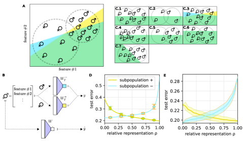
Figure 1: The Teacher-Mixture (T-M) model can account for several types of data imbalance and gives rise to a bias-induction phenomenology compatible with observations in realistic datasets. Panel A The T-M model is a generative model of high-dimensional structured data. Inputs are sampled from a combination of multivariate Gaussian distributions, with different centroids and covariances for each sub-population in the dataset. The probability of sampling from each sub-population can be tuned, giving rise to representation imbalance. In particular, the cartoon shows a larger relative representation for the male population, which also has a smaller variance. Panel B Given a vector of input features and a group membership (male/female), the ground-truth label is assigned by the associated 1-layer teacher network (represented by one of the vectors $W_{T}^{\pm}$). The decision boundaries are demarked in blue and yellow (while their intersection is coloured in green)). The labelling rules can be aligned, i.e. the decision rule does not depend on the group membership, or misaligned as in panel A. A 1-layer student network is given inputs $\boldsymbol{x}^{\mu}$ and labels $y^{\mu}$, and trained to produce the correct outputs $\hat{y}$ via gradient descent on the loss $\ell(\hat{y},y)$. Panel C The panel exemplifies how manipulating the parameters of the T-M model can alter the data distribution: C.1 represents the balanced condition with equally represented, distributed and labelled samples; C.2 shows scarcity of data points in both clusters; C.3 displays an example of rule misalignment; C.4 shows different sub-population variances; C.5 shows relative representation imbalance; C.6 represents the case of unbalanced labels; C.7 shows a case of positive group-label correlation . Panel D shows the training performance of the student network on an instance of the problem as the relative representation is manipulated. Not surprisingly, when one sub-population a largely predominant on the dataset, the classifier will be biased to have higher accuracy on it. The plot shows the match between the analytic curves described in Sec. 2 (solid lines), and numerical simulations on the synthetic framework (dots). Panel E contains a similar experiment, but with data from the ‘CelebA’ dataset [16]. Details in the SI A.

Drug testing provides a historically significant example of the potential consequences of unchecked data imbalance: substantial evidence [17, 18, 8] shows that the scarcity of data points corresponding to female individuals in drug-efficiency studies resulted in a larger number of side effects in their group. This historical data gap has often been justified on the basis of a “simplification” criterion: due to the inherent variance of the female sub-population (caused e.g. by fluctuating hormonal levels), their inclusion in medical trials can introduce complex interactions that are instead absent in the “standard” male sub-population. However, ignoring biological sex as a discriminative factor in the analysis can induce serious adverse effects on the female sub-population, ranging from over-dosage to ineffectiveness of treatment.

The Teacher-Mixture (T-M) model is designed to allow a theoretical characterisation of the impact of such data imbalances on the inference process (e.g., determining a discriminative rule for administering the drug to the patients). While retaining analytical tractability, the T-M model retraces the main features of real data with multiple coexisting sub-populations and allows for a richer phenomenology than previously analysed data models. In panel A of Fig. 1, we sketch a 2-dimensional cartoon of the T-M data distribution, framed in the context of drug testing.

The T-M combines aspects of two common modelling frameworks for supervised learning, namely the Gaussian-Mixture (GM) and the Teacher-Student (TS) setups [19]. The GM is a simple model of clustered input data, where each data point is sampled from one out of a narrow set of high-dimensional Gaussian distributions. Instead, the T-M inherits from the TS setup a simple model of input-label correlation, where the ground-truth labels are produced by a realisable "teacher" rule, to be inferred by the trained model during the learning process. For simplicity, in this study, we will only consider linear labelling rules. In the T-M, however, we allow for the existence of group-specific rules: at inference, the model will have to strike a compromise between them. In the sketch in Fig. 1 A, the female and male sub-populations are represented as partially overlapping data clouds, with different variances and group-dependent offsets (the two features in the sketch could represent some combination of clinical values recorded during the trial). Note that the female population is numerically under-represented, as in the above-described real-world scenarios. The shaded areas represent the true regions of the effectiveness of the tested drug for female/male subjects (cyan/yellow shades). As depicted in panel B, the goal of the inference model is to infer a decision boundary for the administration of the drug based on the observations of its effectiveness on the test subjects. While the vast majority of the subjects would be identically classified according to the two different labelling rules (green region), some false positives could occur if the inference only accounts for a single sub-population.

If no explicit bias mitigation strategy is employed, a heterogeneous representation of the two sub-groups will inevitably lead to a biased inference model. In panels D and E of Fig. 1, we show that the classification accuracy on the two sub-populations, as the fraction of data points belonging to each group (the relative representation) is varied, is biased in favour of the majority group. Many different factors, parametrically controlled in the T-M, can accentuate the impact of the relative representation, as shown in panel C of Fig. 1 and further discussed below.

For simplicity, the results discussed in this paper will focus on the case of two groups, but the analysis could be extended to multiple sub-populations.

Formal definition We consider a synthetic dataset of $n$ samples $\mathcal{D}=\left\{\mathbf{x}^{\mu},y^{\mu}\right\}_{\mu=1}^{n}$, with $\mathbf{x}^{\mu}\in\mathbb{R}^{d}$, $y^{\mu}\in\{1,-1\}$. We define the $\mathcal{O}(1)$ ratio $\alpha=n/d$ and we refer to it as the dataset size parameter. Each input vector is i.i.d. sampled from a mixture of two symmetric Gaussians with variances $\Delta=\{\Delta_{+},\Delta_{-}\}$, $\mathbf{x}\sim\mathcal{N}(\pm\boldsymbol{v}/\sqrt{d},\Delta_{\pm}\mathbb{I}^{d\times d})$, with respective probabilities $\rho$ and $(1-\rho)$. The shift vector $\mathbf{v}$ is a Gaussian vector with i.i.d. entries with zero mean and variance $1$. The $1/\sqrt{d}$ scaling corresponds to the high-noise noise regime, where the two Gaussian clouds are overlapping and hard to disentangle [20, 21], e.g. as in the case of CelebA and MEPS shown in the Supplementary Information (SI) A. The ground-truth labels, instead, are provided by two i.i.d. Gaussian teacher vectors, namely $\mathbf{W}_{T}^{+}$ and $\mathbf{W}_{T}^{-}$, with components of zero mean and variance 1. Each teacher produces labels for the inputs with the corresponding group-membership, namely $y^{\mu}=\mathrm{sign}\left(\mathbf{W}_{T}^{\pm}\cdot\mathbf{x}_{\pm}^{\mu}/\sqrt{d}+b_{T}^{\pm}\right)$. The thresholds $b_{T}^{\pm}$ correspond to the teacher bias terms, included in the model to control the fraction of positive and negative samples within the two sub-populations. Overall, the geometric picture of the data distribution (sketched in Fig. 1) is summarised by three sufficient statics, $\tilde{m}_{\pm}=\frac{1}{d}\boldsymbol{W}_{T}^{\pm}\cdot\boldsymbol{v}$ and $q_{T}=\frac{1}{d}\boldsymbol{W}_{T}^{+}\cdot\boldsymbol{W}_{T}^{-}$, , that respectively quantify the alignment of the teacher labelling rules with respect to the shift vector, controlling the group-label correlation, and the alignment between the teacher vectors, controlling the correlation between labels assigned to similar inputs belonging to different communities.

Given the synthetic dataset $\mathcal{D}$, we study the properties of a single-layer network $\boldsymbol{W}$, with output $\hat{y}^{\mu}=\mathrm{sign}\left(\mathbf{W}\cdot\mathbf{x}_{\pm}^{\mu}/\sqrt{d}+b\right)$, trained via empirical risk minimisation (ERM) with loss:

$$\mathcal{L}(\boldsymbol{W},b_{s})=\sum_{\mu\in\mathcal{D}}\ell\left(\boldsymbol{W},b_{s};\boldsymbol{x}^{\mu},y^{\mu}\right)+\frac{\lambda||\boldsymbol{W}||_{2}^{2}}{2}$$ (1)

where $\ell$ is assumed to be convex in student’s parameters, $\lambda$ is an external parameter that regulates the intensity of the $L_{2}$ regularisation, and the index $c^{\mu}\in\{+,-\}$ denotes the group membership of data point $\mu$.

Given this framework, we derive a theoretical characterisation of the training performance of this learning model and consider the possible implications from an ML fairness perspective. In particular, we aim to study the role of data geometry and cardinality in the training of a fair classifier. To quantify the level of bias in the predictions of the trained model, we need to choose a metric of fairness. We will employ disparate impact (DI) [22], an ML analog of the 80% rule [23], which allows a simple assessment of the over-specialisation of the classifier on one of the sub-populations. In our framework, we characterise bias against sub-population $+$ using the following definition of $DI=p(\hat{y}=y|+)/p(\hat{y}=y|-)$, evaluating the ratio between test accuracy in sub-population $+$ and sub-population $-$. Note that how to measure bias is itself an active line of research, and the DI alone cannot return a full picture of the unfairness. In Sec. 4, we compare these results with those obtained with other metrics. Notice, that the T-M model allows to parametrically move from a model-mismatched scenario ($q_{T}<1$) where the rule to be inferred is not in the function space of learnable rules, to a model-matched scenario ($q_{T}=1$) where the rule is actually learnable but, as we will discuss further in Sec. 3, the model may systematically fail to identify it. We will discuss in detail when these failure modes occur and why.

Finally, the T-M model has, at the same time, the advantage of being simple, allowing a better understanding of the many facets of ML bias, and the disadvantage of being simple, since some modelling assumptions might not reflect the complexity of real-world data. For example, we ignore any type of correlation among the inputs other than the clustering structure. However, this modelling approach continues a long tradition of research in statistical physics [24], which has shown that theoretical insights gained in prototypical settings can often be helpful in disentangling and interpreting the complexity of real-world behaviour.

Remark 1

By looking at the available degrees of freedom in the T-M, several possible sources of bias naturally emerge from the model:

• the relative representation, $\rho=n_{+}/(n_{+}+n_{-})$, with $n_{c}$ the number of points in group $c$.

• the group variance, $\Delta_{c}$, determining the width of the clusters.

• the group label frequencies, controlled through the bias terms $b_{c}$.

• the group-label correlation, $m_{c}$.

• the inter-group similarity, $q_{T}$, which measures the alignment between the two teachers, i.e. the linear discriminators that assign the labels to the two groups of inputs.

• the dataset size, $\alpha$, representing the ratio between the number of inputs and the input dimension.

Theoretical analysis in high-dimensions.

In principle, solving Eq. 1 requires finding the minimiser of a complex non-linear, high-dimensional, quenched random function. However, statistical physics [25] showed that in the limit $n,d\to\infty$, $n/d=\alpha$, a large class of problems, including the T-M model, becomes analytically tractable. In fact, in this proportional high-dimensional regime, the behaviour of the learning model becomes deterministic and trackable due to the strong concentration properties of a narrow set of descriptors that specify the relevant geometrical properties of the ERM estimator. The original high-dimensional learning problem can be reduced to a simple system of equations that depends on a set of scalar sufficient statistics: $Q=\frac{1}{d}\boldsymbol{W}\cdot\boldsymbol{W}$, $m=\frac{1}{d}\boldsymbol{W}\cdot\boldsymbol{v}$, and $R_{\pm}=\frac{1}{d}\boldsymbol{W}\cdot\boldsymbol{W}_{T}^{\pm}$, representing the typical norm of the trained estimator, its magnetisation in the direction of the cluster centres, and its alignment with the two teachers of the T-M.

Analytical result 1

In the high dimensional limit when $n$, $d\to\infty$ at a fixed ratio $\alpha=n/d$, the scalar descriptors $\Theta=\{Q,m,R_{\pm},\delta q\}$ of the vector $\boldsymbol{w}$ obtained by the empirical risk minimisation of Eq. 1 with a convex loss, and their Lagrange multipliers $\hat{\Theta}=\{\hat{Q},\hat{m},\hat{R}_{\pm},\delta\hat{q}\}$, converge to deterministic quantities given by the unique fixed point of the system:
$Q=-2\frac{\partial s(\hat{\Theta};\lambda)}{\partial\,\delta\hat{q}};$ $m=\frac{\partial s(\hat{\Theta};\lambda)}{\partial\,\hat{m}};$ $R_{\pm}=\frac{\partial s(\hat{\Theta};\lambda)}{\partial\,\hat{R}_{\pm}};$ $\delta q=2\frac{\partial s(\hat{\Theta};\lambda)}{\partial\,\hat{Q}};$ $\hat{Q}=2\alpha\frac{\partial e(\Theta;\Delta)}{\partial\,\delta q};$ $\hat{m}=\alpha\frac{\partial e(\Theta;\Delta)}{\partial\,m};$ $\hat{R}_{\pm}=\alpha\frac{\partial e(\Theta;\Delta_{\pm})}{\partial\,R_{\pm}};$ $\delta\hat{q}=2\alpha\frac{\partial e(\Theta;\Delta)}{\partial\,Q}$. with:

$$\begin{split}s&(\hat{\Theta};\lambda)=\frac{1}{2\left(\delta\hat{q}+\lambda\right)}\Bigg{[}\hat{Q}+\left(\hat{m}+\sum_{c\in\{\pm\}}\tilde{m}_{c}\hat{R}_{c}\right)^{2}+\\ &+\sum_{c\in\{\pm\}}(1-\tilde{m}_{c}^{2})\hat{R}_{c}^{2}+2\left(q_{T}-\prod_{c\in\{\pm\}}\tilde{m}_{c}\right)\prod_{c\in\{\pm\}}\hat{R}_{c}\Bigg{]}\end{split}$$ (2)

$$\begin{split}e&(\Theta;\Delta)=\mathbb{E}_{c}\Bigg{[}\mathbb{E}_{z}\\ &\sum_{y=\pm 1}H\left(-y\frac{\sqrt{Q}(c\,\tilde{m}_{c}+\tilde{b}_{c})+\sqrt{\Delta_{c}}R_{c}z}{\sqrt{\Delta_{c}(Q-R_{c}^{2})}}\right)v(y,c,\Theta)\Bigg{]}\end{split}$$ (3)

where $c\in\{+,-\}\sim\mathrm{Bernoulli}(\rho)$, $z\sim\mathcal{N}(0,1)$, $H(\cdot)=\frac{1}{2}\mathrm{erfc}(\cdot/\sqrt{2})$ is the Gaussian tail function, $w$ is the solution of: $v(y,c,\Theta)=\max_{w}\left[-\frac{w^{2}}{2}-\ell\left(y,\sqrt{\Delta_{c}\delta q}w+\sqrt{\Delta_{c}Q}z+c\,m+b\right)\right)]$ and the bias $b$ implicitly solves the equation $\,\,\partial_{b}e(\Theta;\Delta)=0$.

The result was obtained through the non-rigorous yet exact replica method from statistical physics [25, 26, 19]. The derivation details are deferred to the Methods 6.1. We remark that several analytic results obtained through the replica method have been subsequently proved rigorously. In particular, the proofs presented by [27, 20, 28] in settings similar to the present one suggest that an extension for the T-M case could be derived. However, this is left for future work. In this manuscript, we verify the validity of our theory by comparison with numerical simulations, as shown e.g. in the central panel of Fig. 1.

The obtained fixed point for the scalar descriptors $\Theta$ can be used to evaluate simple expressions for common model evaluation metrics, such as the confusion matrix or the generalisation error.

Analytical result 2

In the same limit as in Analytical result 1, the entries of the confusion matrix, representing the probability of classifying as $\hat{y}$ an instance sampled from sub-population $c$ with true label $y$, are given by:

$$\begin{split}p\left(\hat{y}\,|\,y;c\right)=&\mathbb{E}_{z}\Bigg{[}\mathrm{Heav}\left(y\left(\sqrt{\Delta_{c}}z+c\,\tilde{m}_{c}+\tilde{b}_{c}\right)\right)\times\\ &\times H\left(-\hat{y}\frac{(c\,m+b)+\sqrt{\Delta_{c}}R_{c}z}{\sqrt{\Delta_{c}(Q-R_{c}^{2})}}\right)\Bigg{]},\end{split}$$ (4)

where $z\sim\mathcal{N}(0,1)$ and $\mathrm{Heav}(\cdot)$ is the Heaviside step function. The generalisation error, representing the fraction of wrongly labelled instances, can then be obtained as $\epsilon_{g}=\mathbb{E}_{c}\left[\sum_{\hat{y}\neq y}p(\hat{y}\,|\,y;c)\right]$.

This second yields a fully deterministic estimate of the accuracy of the trained model on the different data sub-populations. These scores will be used in the following sections to investigate the possible presence of bias in the classification output of the model. Note that the results 1 and 2 allow for an extremely efficient and exact evaluation of the learning performance in the T-M, remapping the original high-dimensional optimisation problem onto a system of deterministic scalar equations that can be easily solved by recursion.

3 Investigating the sources of bias

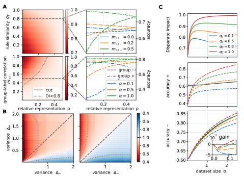
Figure 2: Simple geometrical properties cause the emergence of bias but data correlation can lead to benefit in classification of both subpopulations. Panel A Each point in the left diagrams shows, for different values of the model parameters, the Disparate Impact (DI) of the trained model (darker colours represent stronger biases). In particular, in the left upper (lower) diagram, on the x-axis we vary the relative representation $\rho$, while on the y-axis we explore possible values of the rule similarity $q_{T}$ (group-label correlation $m_{\pm}$). The corresponding figures on the right show the values of the accuracy for the two sub-populations in correspondence of the cut represented by the dashed line on the left. Panel B We show the disparate impact as the distribution of the two subpopulations is changed by altering their variances ($\Delta_{+}$ and $\Delta_{-}$). The diagonal line gives the configurations where the two subpopulations have the same variance. The two figures consider different levels of representation, from left to right $\rho=0.1,0.5$. The latter is the situation with both subpopulations being equally represented in the dataset. We use the red and blue colours to quantify the disparate bias against sub-population $+$ and $-$ (respectively). Panel C With $10\%$ of the data points in sub-population $+$ ($\rho=0.1$), we compare the performance with different levels of rule similarity ($q_{T}$) as the size of the dataset is increased, showing the disparate impact in the upper figure and the individual accuracies in central and lower ones. In central and lower figures, the baselines –plotted in black– show the accuracies attained when the model is trained only on the corresponding group data. The inset of the lower figure highlights the differences in accuracy in the small dataset regime. When the rules are sufficiently aligned, joint training on both groups will induce a better accuracy on the smaller sub-population provided $\alpha$ is not too small. Moreover, at intermediate values of $\alpha$ also the larger group can benefit from the information transfer.

FAIRNESS METRIC	CONDITION
Statistical Parity	$\mathbb{P}[\hat{Y}=y|C=c]=\mathbb{P}[\hat{Y}=y]\;\forall y,c$
Equal Opportunity	$\mathbb{P}[\hat{Y}=1|C=c,Y=1]=\mathbb{P}[\hat{Y}=1|Y=1]\;\forall c$
Equal Accuracy	$\mathbb{P}[\hat{Y}=y|C=c,Y=y]=\mathbb{P}[\hat{Y}=y|Y=y]\;\forall y,c$
Equal Odds	$\mathbb{P}[\hat{Y}=1|C=c,Y=1]=\mathbb{P}[\hat{Y}=1|Y=1]\ \cap$ $\mathbb{P}[\hat{Y}=1|C=c,Y=-1]=\mathbb{P}[\hat{Y}=1|Y=-1]\;\forall c$
Predicted Parity	$\mathbb{P}[Y=1|C=+,\hat{Y}=y]=\mathbb{P}[Y=1|C=-,\hat{Y}=y]$ $=\mathbb{P}[Y=1|\hat{Y}=y]\;\forall y$

Table 1: List of Fairness Metrics. Statistical Parity: Equal fractions of each group should be treated as belonging to the positive class [29, 30, 31]. Equal Opportunity: Each group needs to achieve equal true positive rate[32]. Equal Accuracy: Each group is required to achieve the same level of accuracy. Equal Odds: Each group should achieve equal true positive and false positive rates[22, 33]. Predicted Parity. Given inputs that are classified by the model with label $y$, the fraction of input with true label $y^{*}$ should be consistent across sub-populations. This gives two sub-criteria: predicted parity 1 requires the condition only for $y^{*}=1$, while predicted parity 10 requires the condition for both $y^{*}=1$ and $y^{*}=-1$ [34].

With these analytical results in hand, we now turn to systematically investigating the effect of the sources of bias identified in remark 1, which potentially mine the design of a fair classifier. We consider three separate experiments to summarise some distinctive features of the fairness behaviour in the T-M: namely, the impact of the correlation between the labelling rules and the group structure, the interplay between relative representation and group variance, and the different accuracy trade-offs between the sub-populations at different dataset sizes. The parameters of the experiments, if not specified in the caption, are detailed in the Methods 6.2.

Group-label correlation.

In the two upper panels of Fig. 2a, we consider a scenario where the labelling rules for the two groups are not perfectly aligned, i.e. $\boldsymbol{W}_{T}^{+}\neq\boldsymbol{W}_{T}^{-}$ (and/or $b_{+}\neq b_{-}$). Note that, in this case, we have a clear mismatch between the learning model, a single linear classifier, and the true input-output structure in the data: the learning model cannot reach perfect generalisation for both sub-populations at the same time. For simplicity, we set an equal correlation between the two teacher vectors and the shift vector, $m_{+}=m_{-}>0$, and isolate the role of rule similarity $q_{T}$. The upper-left panel shows a phase diagram of the DI (DI$<1$ indicating a lower accuracy on group $+$), as function of the similarity of the teachers and the fraction of $+$ samples in the dataset. As intuitively expected, the induced bias exceeds the 80% rule when the labelling rules are misaligned and the group sizes are numerically unbalanced (small $q_{T}$ and $\rho$). Indeed, in the cut displayed in the upper-right panel, by lowering the group-label correlation $m_{\pm}$ the gap between the measured accuracies on the two sub-populations becomes smaller. However:

Remark 2

Even when $q_{T}=1$ and the task is solvable (i.e. the classifier can learn the input-output mapping), the trained model can still be biased.

This is shown in the two lower panels of Fig. 2a, where a large high-bias region (DI$<80$%) exists. In particular, the lower-left panel shows the cause of this effect in the presence of a non-zero group-label correlation $m_{\pm}$, and in the lower-right panel we see how this effect is more pronounced in the data-scarce regime. In all four panels, as $\rho$ reaches $0.5$, the two sub-populations become equally represented and the classifier achieves the same accuracy for both.

Bias and variance.

In Fig. 2b, we plot the DI as a function of the group variances $\Delta_{\pm}$, for different values of the fraction of $+$ samples. One finds that the model might need a disproportionate number of samples in the two groups to obtain comparable accuracies. We can see that:

Remark 3

Balancing the group relative representation does not guarantee a fair training outcome.

In fact, the quality of a group’s representation in the dataset can increase if the number of points is kept constant but the group variance is reduced. The blue regions in the left panel indicate a higher accuracy for the smaller sub-population even if the dataset only contains $10\%$ of samples belonging to it. This exemplifies the fact that a very focused distribution (low $\Delta_{\pm}$) actually requires less samples. The right panel ($\rho=0.5$) shows the scenario one would expect a priori: on the diagonal line the DI is balanced, but by setting $\Delta_{+}>\Delta_{-}$ (or viceversa) one induces a bias in the classification.

Positive transfer.

If mixing different sub-populations in the same dataset can induce unfair behaviour, one could think of splitting the data and train independent models. In Fig. 2c, we show that a positive transfer effect [35] can yet be traced between the two groups when the rules are sufficiently similar. This means that the accuracy on the under-represented group is enhanced when information is shared across the two sub-populations.

Remark 4

The performance on the smaller sub-population tends to further deteriorate if the dataset is split according to the sub-group structure.

To clarify this point, in the top plot of Fig. 2c we show the DI as a function of the dataset size $\alpha$, for several values of the rule similarity $q_{T}$ and at fixed $\rho=0.10$. In the middle and bottom plots in Fig. 2c, we also display the gain in accuracy on each sub-population when the model is trained on the full dataset, comparing with a baseline classifier (black lines) trained only on the respective data subsets ($+$ in the central panel, $-$ in the lower panel). These two plots elucidate the positive transfer effect: for sufficiently similar rules (large $q_{T}$), both populations can benefit from shared training at intermediate dataset sizes. If the dataset is too small (low $\alpha$ regime), the lack of data combined with a high variance in the input distribution can induce over-fitting, with a larger drop in performance for the smaller group. On the other hand, as the dataset size becomes sufficiently large, the positive transfer effect is eventually lost for the large sub-population (large $\alpha$ regime). Connecting the results of this section to the drug testing examples, after observing that the distribution of side effects in the female population presented a larger variance, the solution was simply to collect more data of female subjects. Moreover, the results shown in Fig. 2b indicate the need for a higher relative representation of female subjects in the dataset to achieve an unbiased classifier. While implementing this solution might have introduced higher variance in the results due to the intrinsic high-variability of the data, it would have significantly reduced the risk of administering drugs with limited testing on half of the population.

4 Mitigation strategies

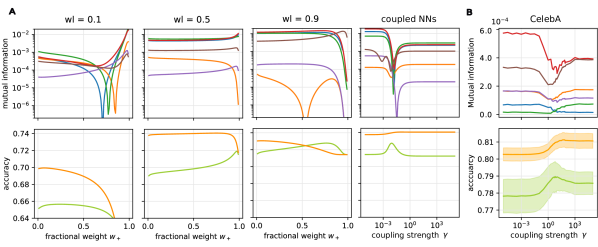
Figure 3: Fairness-accuracy trade-off with reweighing and coupled architecture. Panel A The figures show the effect of re-weighting and coupled architectures de-biasing methods in a instance of the T-M model. The lowers figures shows the accuracy for subpopulation $+$ and subpopulation $-$ and the upper figures show the mutual information for the several fairness metrics defined in Table 1, namely statistical parity, equal opportunities, equal accuracy, equal odds, predicted parity $1$, and predicted parity $10$. The goal of the algorithm is to identify regions with high accuracy (lower figures) and low mutual information (higher figures) for all metrics: this would imply that fairness is approximately achieved under all the criteria. The first three group of figures refer to the reweighing strategy, forcing higher relevance for a certain label in each panel ($w_{1}=0.1,0.5,0.9$) and the relative importance of a given subpopultation (parameter $w_{+}$) on the x-axis. The last panels instead refer to the proposed coupled networks strategy and the x-axis represent the strength of the coupling $\gamma$. The figures clearly show that our strategy achieves a higher accuracy in both subpopulations while preserving a higher level of fairness. Interestingly the minimum of the mutual information roughly correspond to the same parameter of the coupling strength, contrarily to what observed in the reweighing strategy. Panel B The two panels, show an example from the CelebA dataset splitting and classifying according to the attributes “Wearing_Lipstick” and “Wavy_Hair” respectively, more details are provided in the SI A.1 and A. The observations made for the synthetic model applies also in this real-world case.

To assess or ensure the fairness of a ML model on a given data distribution, a plethora of different fairness criteria have been designed [36, 37]. In convex settings, any of these criteria can be separately enforced via a hard constraint during the optimisation process [38, 39, 40]. However, it was proved that some criteria are completely incompatible and cannot be exactly achieved simultaneously [30, 41, 42]. In the same spirit of [36], we drop the hard constraint and instead quantify exactly how far a given trained model is from meeting the criteria. Each criterion requires the probability of obtaining a specific classification outcome $E$ to be the same across the sub-populations. For example, according to the definition of Equal Opportunity (Table 1), the true positive rate $P(E=(\hat{Y}=1\,|\,Y=1))$ should not depend on the group-membership $C$. A natural measure of the observed dependence between $E$ and $C$ is given by the Mutual Information (MI):

$$I(E;C)=D_{KL}(\mathbb{P}[E,C]\ \big{|}\ \mathbb{P}[E]\mathbb{P}[C])=\mathbb{E}\log\frac{\mathbb{P}[E,C]}{\mathbb{P}[E]\mathbb{P}[C]}.$$ (5)

The fairness condition is exactly verified only when the joint distribution factorizes, i.e. $\mathbb{P}[E,C]=\mathbb{P}[E]\mathbb{P}[C]$, and the mutual information goes to zero. Table 1 provides some other examples of classification events $E$, for some well-established fairness criteria. Note that some criteria might not be sensible in specific settings (e.g., Statistical Parity is unlikely to be guaranteed in a drug-testing scenario).

In the following, we consider two simple bias mitigation strategies that can be analysed within our analytical framework. The required generalisations of the results shown in Sec. 2 are detailed in the Methods 6.1. First, we study the de-biasing effect of a sample reweighing strategy where the relevance of each sample is varied based on its label and group membership [43, 44, 45]. By adjusting the weights, one can indirectly minimise the MI relative to any given fairness measure. We use the simultaneous quantitative predictions on the various metrics to assess the compatibility between different fairness definitions. Then, we propose a theory-based mitigation protocol, along the lines of protocols used in the context of multi-task learning [46], that couples two architectures trained in parallel.

Loss Reweighing.

Recent literature shows that some fairness constraints cannot be satisfied simultaneously. ML systems are instead forced to accept trade-offs between them [30]. This sort of compromise is well-captured in the simple framework of the T-M model. The first three panels of Fig. 3a show accuracies and MI measured with respect to the various fairness criteria while varying the two reweighing parameters, $w_{1}$ and $w_{+}$, which up-weigh data points with true label $1$ and in group $+$, respectively. Thus, each loss term in Eq. 1 is reweighed as:

$$\mathcal{W}(c,y)=\begin{cases}w_{1}w_{+}&\text{if}\quad c=+,y=1\\ w_{1}(1-w_{+})&\text{if}\quad c=-,y=1\\ (1-w_{1})w_{+}&\text{if}\quad c=+,y=-1\\ (1-w_{1})(1-w_{+})&\text{if}\quad c=-,y=-1\,.\\ \end{cases}$$ (6)

By changing these relative weights one can force the model to pay more attention to some types of errors and re-establish a balance between the accuracies on the two sub-populations. The goal is to identify a classifier that achieves high accuracy (lower panels) while minimising the MI for different fairness metrics. Notably, given a weight $w_{1}$, these minima occur for different values of the weight $w_{+}$. Only $w_{1}=0.1$ seems to have a value of $w_{+}$ close to several minima of the MI, but this point correspond to a sharp decrease in accuracy in both subpopulations, thus fairness is achieved but at the expense of accuracy. These results are in agreement with rigorous results in the literature [42], but also show how the incompatibilities between the different constraints extend to regimes where the fairness criteria are not exactly satisfied.

Coupled Networks.

The emergence of classification bias in the T-M traces back to the clear mismatch between the generative model of data and the learning model. In order to move towards a matched inference setting, we need to enhance the learning model to account for the presence of multiple sub-populations and labelling rules. This inspires a novel mitigation strategy – that we call coupled neural networks – consisting in the simultaneous training of multiple neural networks, each one seeing a different subset of the data associated with a different sub-population. This idea is represented by the following modified loss

$$\begin{split}&\mathcal{L}_{\text{cnn}}(\boldsymbol{w})=\sum_{c\in{\pm}}\sum_{\mu\in\mathcal{D}^{c}}\ell\left(\boldsymbol{W_{c}},b_{s,c};\boldsymbol{x}^{\mu},y^{\mu}\right)\\ &\quad+\frac{\lambda}{2}\left(||\boldsymbol{W}_{+}||_{2}^{2}+||\boldsymbol{W}_{-}||_{2}^{2}\right)+\frac{\gamma}{2}||\boldsymbol{W}_{+}-\boldsymbol{W}_{-}||_{2}^{2}\end{split}$$ (7)

where $\boldsymbol{W}_{\pm}$ are the weights of the two networks and $\hat{y}_{\pm}^{\mu}$ are their respective estimation of label $y^{\mu}$. The networks exchange information by means of the elastic penalty $\gamma$ that mutually attracts them, and the intensity of this elastic interaction is obtained by cross-validation. This approach shares some ideas with other methods present in the literature: [47, 48] add an elastic penalty term to the loss to bias the training trajectory, while [49] proposes to combine estimations from different Bayesian classifiers. However, note that these prior approaches were tailored for different learning protocols or problem domains, and could not be applied in the problem setting considered in this paper.

Remark 5

The coupled neural networks method allows for higher expressivity and specialisation on the various sub-populations, while also encouraging positive transfer between similarly labelled sub-populations, leading to better fairness-accuracy trade-offs.

The upper rightmost plots of Fig. 3a, displaying the behaviour of the mutual information as a function of the coupling parameter for different fairness metrics, shows the key advantage of using this method. We observe a more robust consistency among the various fairness metrics: the positions of the different minima are now very close to each other. Moreover, the value of the coupling parameter achieving this agreement condition is also the one that minimises the gap in terms of test accuracy between the two sub-populations, as shown in the lower plot, without hindering the performance on the larger group. Notice that this result does not contradict the impossibility theorem [42] which states that statistical parity, equal odds, and predicted parity cannot be satisfied altogether. In fact, our result only concerns soft minimisation of each fairness metrics. The result is in agreement with [50] whose results show that the trade-off between fairness and accuracy vanishes when the true distribution of data is capture. Leveraging the universal approximation property of neural networks, the coupled networks method seems a promising direction for applications. In the panels of Fig. 3b we show promising preliminary results in the realistic dataset CelebA. We stress that real data often presents more complex correlations than those modelled in the T-M, which may hinder the effectiveness of this strategy in unexpected ways.

The method of the coupled networks can be generalised to an arbitrary number of classes and sub-populations, and can be combined with standard clustering methods when the group membership label is not available. A future research direction will be to better investigate its range of applicability and, consequently, its limitations in real-world scenarios. In the Methods 6.1 and in the SI C we provide additional results for this method and we discuss the effect of training the networks on data subsets that only partially correlate with the true group structure.

5 Discussion

The goal of this study was to design a novel generative model of high-dimensional correlated data that allows the study of the effect of data geometry in the bias induction mechanism, in isolation from real-world confounding factors. While a focus on each specific dataset might be required to ensure fairness in applications with high societal impact, we believe that the study of the ML bias phenomenology in controlled synthetic settings might allow more coherent advancements in the understanding and prevention of bias induction.

The Teacher-Mixture (T-M) model captures non-trivial correlations among inputs and between inputs and labels, representing various imbalances appearing in real datasets when different sub-populations coexist in the sample. Surprisingly, with few modelling ingredients, the T-M can generate a rich and realistic ML bias phenomenology. We derive an analytical characterisation of its performance in the high-dimensional limit, showing agreement with numerical simulations and producing realistic unfairness behaviour. By isolating different sources of bias, we gain insights into situations where unfairness may persist despite apparent data balance, cautioning against relying solely on simple rebalancing techniques. We identify a positive transfer effect among diverse sub-populations, leveraging shared underlying features to enhance performance across groups.

Additionally, we analyzed the trade-offs between different ways of quantifying the model fairness, focusing on a sample reweighing mitigation strategy that can be analytically characterised within our framework. We also proposed a theory-based mitigation strategy that effectively promotes fairness without compromising overall performance, as demonstrated in the T-M model. Instead of imposing an hard constraint on a desired fairness metric which would incur in the incompatibility theorem [42], the coupled networks strategy minimises several fairness metrics simultaneously only approximately. Furthermore, the strategy seems to avoid the typical fairness-accuracy trade-off. This result is in agreement with the findings of [50] showing that it is possible to construct a Bayes optimal classifier that is not affected by the trade-off.

Future directions for our research include incorporating more complex elements into the data model, such as exploring the multi-label classification case [51] and the effect of feature dependencies (e.g., proxy variables) in the generated data. Another important but challenging address for further work is to move to the non-convex optimisation setting and to more complex model architectures, where at this time some of the analytic techniques employed in this work fail to generalise. Moreover, further explorations of the efficacy and limitations of the coupled networks strategy in the context of deep networks and more complex datasets is called for. By investigating its performance in deeper architectures and diverse real-world datasets, and connecting to the existing literature [52, 53], we can assess the scalability and generalisability of this approach for addressing fairness concerns.

6 Methods

6.1 Replica analysis

We will directly present the most general setting for this calculation, where the learning model is composed of two linear classifiers (“students” in the following), coupled by an elastic penalty of intensity $\gamma$. This allows us to characterise the novel mitigation strategy proposed in this work, while the standard case with a single learning model can be obtained by setting $\gamma=0$. Each student, denoted by the index $s=1,2$, is assumed to be trained on a fraction of the full dataset $\mathcal{D}_{s}$. Note that, in principle, the data split could not be aligned with the group structure of the dataset.

The loss function for the coupled learning model reads:

$$\mathcal{L}(\boldsymbol{W}_{1},\boldsymbol{W}_{2})=\sum_{s=1,2}\sum_{\mu\in\mathcal{D}_{s}}\ell\left(\frac{\boldsymbol{W}_{T}^{c^{\mu}}\cdot\boldsymbol{x}^{\mu}}{\sqrt{d}}+\tilde{b}_{c^{\mu}},\frac{\boldsymbol{W}_{s}\cdot\boldsymbol{x}^{\mu}}{\sqrt{d}}+b_{s}\right)+\sum_{s=1,2}\frac{\lambda}{2}\left(\sum_{i=1}^{d}W_{s,i}^{2}\right)-\frac{\gamma}{2}\lVert\boldsymbol{W}_{1}-\boldsymbol{W}_{2}\rVert^{2}$$ (8)

and we will focus in the following on the cross-entropy loss:

$$\ell(y,q)=-\mathrm{Heav}\left(y\right)\log\sigma(q)-\left(1-\mathrm{Heav}\left(y\right)\right)\log\text{$\left(1-\sigma(q)\right)$}$$ (9)

where $\mathrm{Heav}(\cdot)$ is the Heaviside step function, which outputs $1$ for positive arguments and $0$ for negative ones, and $\sigma\left(x\right)=\left(1+\exp\left(-x\right)\right)^{-1}$ is the sigmoid activation function. The calculation also holds for alternative convex losses, e.g. the Hinge loss or the MSE loss, since the only affected part is the numerical optimisation of the proximal operator, as shown below.

Teacher partition function

In the T-M model, the label distribution is non-trivially dependent on the mutual alignment of the shift vector $\boldsymbol{v}$, determining the means of the two Gaussians in the input mixture, and the two teacher vectors $\boldsymbol{W}_{T}^{\pm}$. Since we are allowed to fix a Gauge for one of these vectors (compatible with its distribution), we choose for simplicity $\boldsymbol{v}=\boldsymbol{1}$ to be a vector with all entries equal to $1$ (still normalized on the sphere of radius $d$). We define the teacher partition function:

$$Z_{T}=\int d\mu(\boldsymbol{W}_{T}^{+},\boldsymbol{W}_{T}^{-})=\int\prod_{c=\pm}\left[d\mu\left(\boldsymbol{W}_{T}^{c}\right)\delta\left(\left|\boldsymbol{W}_{T}^{c}\right|^{2}-d\right)\delta\left(\boldsymbol{W}_{T}^{c}\cdot\boldsymbol{1}-d\tilde{m}_{c}\right)\right]\delta\left(\boldsymbol{W}_{T}^{+}\cdot\boldsymbol{T}_{-}-d\,q_{T}\right),$$

where the measures $\mu({\boldsymbol{T_{\pm}}})$ are in this case assumed to be factorised normal distributions. The Dirac’s $\delta$-functions ensure that the geometrical disposition of the model vectors is the one defined by the chosen magnetisations $\tilde{m}_{\pm}$ and the overlap $q_{T}$, and that the vectors are normalised to the $d$-sphere.

At this point, and throughout this section, we use the integral representation of the $\delta$-function:

$$\delta(x-ad)=\int\frac{d\hat{a}}{2\pi/d}e^{-i\hat{a}\left(\frac{x}{d}-a\right)},$$ (10)

where $\hat{a}$ is a so-called conjugate field that plays a role similar to a Lagrange multiplier, enforcing the constraint contained in the $\delta$-function. We can rewrite:

$$Z_{T}=\int\prod_{c=\pm}\frac{d\hat{Q}_{T}^{c}}{2\pi/d}\int\prod_{c=\pm}\frac{d\hat{\tilde{m}}_{c}}{2\pi/d}\int\frac{d\hat{q}_{T}}{2\pi/d}e^{d\,\Phi_{T}\left(\{\tilde{m}_{\pm},q_{T}\},\{\hat{Q}_{T}^{\pm},\hat{\tilde{m}}_{\pm},\hat{q}_{T}\}\right)},$$ (11)

where the action $\Phi_{T}$ represents the entropy of configurations for the teacher that satisfy the chosen geometrical constraints. Given that the components of the teacher vectors are i.i.d., the entropy can be factorised over them. In high dimensions, i.e. when $d\to\infty$, the integral will be dominated by "typical" configurations for the vectors, and the integral $Z_{T}$ can be computed through a saddle-point approximation. We Wick rotate the fields in order to avoid dealing explicitly with imaginary quantities, and decompose $\Phi_{T}=g_{Ti}+g_{Ts}$:

$$g_{Ti}=-\left(\sum_{c}\hat{\tilde{m}}_{c}\tilde{m}_{c}+\sum_{c}\hat{Q}_{T}^{c}+\hat{q}_{T}q_{T}\right),$$ (12)

$$g_{Ts}=\log\int\mathcal{D}T_{+}\int\mathcal{D}T_{-}\exp\left(\sum_{c}\hat{Q}_{T}^{c}T_{c}^{2}+\sum_{c}\hat{\tilde{m}}_{c}T_{c}+\hat{q}_{T}T_{+}T_{-}\right).$$

After a few Gaussian integrations the computation of the second term yields:

$$g_{Ts}=\frac{\left(1-2\hat{Q}_{T}^{-}\right)\hat{\tilde{m}}_{+}^{2}+\left(1-2\hat{Q}_{T}^{+}\right)\hat{\tilde{m}}_{-}^{2}+2\hat{q}_{T}\hat{\tilde{m}}_{+}\hat{\tilde{m}}_{-}}{2\left(\left(1-2\hat{Q}_{T}^{-}\right)\left(1-2\hat{Q}_{T}^{+}\right)-\hat{q}_{T}^{2}\right)}-\frac{1}{2}\log\left(\left(1-2\hat{Q}_{T}^{+}\right)\left(1-2\hat{Q}_{T}^{-}\right)-\hat{q}_{T}^{2}\right).$$

Now, in order to complete the computation of the partition function $Z_{T}$, we have impose the saddle point condition for $\Phi_{T}$, which is realised when the entropy is extremised with respect to the fields we introduced. From the associated saddle point equations one can find two useful identities:

$$1-\tilde{m}_{c}^{2}=\frac{\left(1-2\hat{Q}_{T}^{-c}\right)}{\left(\left(1-2\hat{Q}_{T}^{-}\right)\left(1-2\hat{Q}_{T}^{+}\right)-\hat{q}_{T}^{2}\right)}$$ (13)

$$q_{T}-\tilde{m}_{+}\tilde{m}_{-}=\frac{\hat{q}_{T}}{\left(\left(1-2\hat{Q}_{T}^{-}\right)\left(1-2\hat{Q}_{T}^{+}\right)-\hat{q}_{T}^{2}\right)}$$ (14)

Free entropy of the learning model

In this subsection we aim to achieve analytical characterisation of typical learning performance in the T-M, i.e. to describe the solutions of the following optimisation problem:

$$\boldsymbol{W}_{1}^{\star},\,\boldsymbol{W}_{2}^{\star}=\underset{\boldsymbol{W}_{1},\,\boldsymbol{W}_{2}}{\mathrm{argmin}}\,\,\mathcal{L}(\boldsymbol{W}_{1},\,\boldsymbol{W}_{2};\mathcal{D}),$$ (15)

where $\mathcal{D}$ represents a realisation of the data and $\mathcal{L}(\cdot)$ was defined in Eq. 8. In typical statistical physics fashion, we can associate this problem with a Boltzmann-Gibbs probability measure, over the possible configurations of the student model parameters:

$$P(\boldsymbol{W}_{1},\,\boldsymbol{W}_{2};\mathcal{D})=\frac{e^{-\beta\mathcal{L}(\boldsymbol{W}_{1},\,\boldsymbol{W}_{2};\mathcal{D})}}{Z_{W}},$$ (16)

where the loss $\mathcal{L}$ plays the role of an the energy function, $\beta$ is an inverse temperature and $Z_{W}$ is the partition function (normalisation of the Boltzmann-Gibbs measure).

Since the loss is convex in the student parameters, when the inverse temperature is sent to infinity, $\beta\to\infty$, the probability measure focuses on the unique minimiser of the loss, representing the solution of the learning problem. In the asymptotic limit $d\to\infty$, the behaviour of this model becomes predictable since the overwhelming majority of the possible dataset realisations (with the same configuration of the generative parameters) will produce solutions with the same macroscopic properties (norm, test performance, etc). We therefore need to consider a self-averaging quantity, which is independent of the specific realisation of the dataset so that the typical learning scenario can be captured.

Thus, we aim to compute the average free-energy:

$$\Phi_{W}=\lim_{d\to\infty}\lim_{\beta}\frac{1}{\beta d}\left<\log Z_{W}(\boldsymbol{W}_{1},\boldsymbol{W}_{2};\mathcal{D}_{1},\mathcal{D}_{2})\right>_{\mathcal{D}_{1},\mathcal{D}_{2}}.$$ (17)

This type of quenched average is not easily computed because of the $\log$ function in the definition. The replica trick, based on the simple identity $\lim_{r\to 0}(x^{r}-1)/r=log(x)$, provides a method to tackle this computation. One can replicate the partition function, introducing $r$ independent copies of the original system. Each of them, however, sees the same realisation of the data $\mathcal{D}$ (the "disorder" of the system, in the statistical physics terminology). When one takes the average over $\mathcal{D}$, the $r$ replicas become effectively coupled, and can be intuitively interpreted as i.i.d. samples from the Boltzmann-Gibbs measure of the original problem. At the end of the computation, one takes the analytic continuation of the integer $r$ to the real axis and computes the limit $\lim_{r\to 0}$, re-establishing the logarithm and the initial expression.

We start by computing the replicated volume (product over the $r$ partition functions) $\Omega^{r}(\mathcal{D})$, which is still explicitly dependent on the sampled dataset:

$$\Omega^{r}(\mathcal{D})=\int\frac{d\mu(\boldsymbol{W}_{T}^{+},\boldsymbol{W}_{T}^{-})}{Z_{T}}\int\prod_{s,a}\left[db_{s}^{a}d\boldsymbol{W}_{s}^{a}e^{-\frac{\beta\gamma}{2}\lVert\boldsymbol{W}_{1}^{a}-\boldsymbol{W}_{2}^{a}\rVert^{2}}\prod_{\mu\in\mathcal{D}_{s}}e^{-\beta\,\ell\left(\frac{\boldsymbol{W}_{T}^{c^{\mu}}\cdot\boldsymbol{x}^{\mu}}{\sqrt{d}}+\tilde{b}_{c^{\mu}},\frac{\boldsymbol{W}_{s}^{a}\cdot\boldsymbol{x}^{\mu}}{\sqrt{d}}+b_{s}^{a}\right)}\right],$$ (18)

where $s=1,2$ indexes the two coupled student models and $a=1,...,r$ is the replica index.

To make progress we have to take the disorder average, i.e. the expectation over the distribution of $\boldsymbol{x}^{\mu}$ as defined in the T-M model. We can exploit $\delta$-functions in order to replace with dummy variables, $u_{\mu}$ and $\lambda^{a}_{\mu}$, the dot products in the loss and isolate the input dependence in simpler exponential terms:

$$1=\int\prod_{\mu}du_{\mu}\,\delta\left(u_{\mu}-\frac{\boldsymbol{W}_{T}^{c^{\mu}}\cdot\boldsymbol{x}^{\mu}}{\sqrt{d}}\right)\int\prod_{a,s,\mu\in\mathcal{D}_{s}}d\lambda_{\mu}^{a}\delta\left(\lambda_{\mu}^{a}-\frac{\boldsymbol{W}_{s}^{a}\cdot\boldsymbol{x}^{\mu}}{\sqrt{d}}\right)$$ (19)

$$=\int\prod_{\mu}\frac{du_{\mu}d\hat{u}_{\mu}}{2\pi}e^{i\hat{u}_{\mu}\left(u_{\mu}-\sum_{i=1}^{d}\frac{W_{T,i}^{c^{\mu}}x_{i}^{\mu}}{\sqrt{d}}\right)}\int\prod_{a,s,\mu\in\mathcal{D}_{s}}\frac{d\lambda_{\mu}^{a}d\hat{\lambda}_{\mu}^{a}}{2\pi}e^{i\hat{\lambda}_{\mu}^{a}\left(\lambda_{\mu}^{a}-\sum_{i=1}^{d}\frac{W_{s,i}^{a}x_{i}^{\mu}}{\sqrt{d}}\right)}$$ (20)

We can now evaluate the expectation over the input distribution, collecting all the terms where each given input appears. By neglecting terms that vanish in the $N\to\infty$ limit, for each pattern $\mu$ we get:

$$\mathbb{E}_{\boldsymbol{x}^{\mu}}e^{-i\sum_{a}\hat{\lambda}_{a}^{\mu}\sum_{i=1}^{N}\frac{W_{s^{\mu},i}^{a}x_{i}^{\mu}}{\sqrt{d}}-i\hat{u}_{\mu}\sum_{i=1}^{d}\frac{W_{T,i}^{c^{\mu}}x_{i}^{\mu}}{\sqrt{d}}}=$$

$$= \prod_{i=1}^{N}e^{-ic^{\mu}\left(\sum_{a}\hat{\lambda}_{a}^{\mu}\frac{W_{s^{\mu},i}^{a}v_{i}}{d}+\hat{u}^{\mu}\frac{W_{T,i}^{c^{\mu}}v_{i}^{\mu}}{d}\right)}\mathbb{E}_{z_{i}^{\mu}}e^{-i\left(\sum_{a}\hat{\lambda}_{a}^{\mu}\frac{W_{s^{\mu},i}^{a}}{\sqrt{d}}+\hat{u}_{\mu}\frac{W_{T,i}^{c^{\mu}}}{\sqrt{d}}\right)z_{i}^{\mu}}$$

$$=e^{-ic^{\mu}\left(\sum_{a}\hat{\lambda}_{a}^{\mu}\frac{\sum_{i}W_{s^{\mu},i}^{a}}{d}+\hat{u}^{\mu}\frac{\sum_{i}W_{T,i}^{c^{\mu}}}{d}\right)-\frac{\Delta_{c^{\mu}}}{2}\left(\sum_{ab}\hat{\lambda}_{a}^{\mu}\hat{\lambda}_{b}^{\mu}\frac{\sum_{i}W_{s^{\mu},i}^{a}w_{s^{\mu},i}^{b}}{d}+2\hat{u}^{\mu}\sum_{a}\hat{\lambda}_{a}^{\mu}\frac{\sum_{i}W_{s^{\mu},i}^{a}W_{T,i}^{c^{\mu}}}{d}+\left(\hat{u}^{\mu}\right)^{2}\frac{\sum_{i}(W_{T,i}^{c^{\mu}})^{2}}{d}\right)}.$$ (22)

To get Eq. 22, we used the fact that the noise $\boldsymbol{z}^{\mu}$ is i.i.d. sampled from centred Gaussians of variance determined by the group, and explicitly used our Gauge choice $\boldsymbol{v}=\boldsymbol{1}$. In this expression we the relevant order parameters of the model appear, describing the overlaps between the student vectors, the shift vector and the teacher vectors. We are thus going to introduce via $\delta$-functions the following parameters:

• $m_{s}^{a}=\frac{\boldsymbol{W}_{s}^{a}\cdot\boldsymbol{1}}{d}$, $\tilde{m}_{c}=\frac{\boldsymbol{W}_{T}^{c}\cdot\boldsymbol{1}}{d}$: magentisations in the direction of the $+$ group centre of the students and the teachers.

• $q_{s}^{ab}=\frac{\sum_{i}w_{si}^{a}w_{si}^{b}}{d}$: self-overlap between different replicas of each student.

• $R_{sc}^{a}=\frac{\sum_{i}W_{s,i}^{a}W_{T,i}^{c}}{d}$: overlap between student and teacher vectors.

• $q_{T}^{c}=\frac{\sum_{i}T_{ci}^{2}}{d}$: norm of the teacher vectors (equal to $1$ by assumption).

After the introduction of these order parameters (via the integral representation of the $\delta$-function) the replicated volume can be expressed as:

$$\Omega^{d}=\int\prod_{s,a}\frac{dm_{s}^{a}d\hat{m}_{s}^{a}}{2\pi/d}\int\prod_{sc,a}\frac{dR_{sc}^{a}d\hat{R}_{sc}^{a}}{2\pi/d}\int\prod_{s,ab}\frac{dq_{s}^{ab}d\hat{q}_{s}^{ab}}{2\pi/d}\int\prod_{c}db_{c}^{a}G_{I}^{d}G_{S}^{d}\prod_{sc}G_{E}(s,c)^{\alpha_{c,s}d}$$ (23)

where $\alpha_{c,s}N$ indicates the number of patterns from group $c$ contained in the data slice $\mathcal{D}_{s}$ given to student $s$. We also introduced the interaction, the entropic and the energetic terms:

$$G_{I}=\exp\left(-N\left(\sum_{s,a}\hat{m}_{s}^{a}m_{s}^{a}+\sum_{s,ab}\hat{q}_{s}^{ab}q_{s}^{ab}+\sum_{sc,a}\hat{R}_{sc}^{a}R_{sc}^{a}\right)\right)$$ (24)

$$G_{S}=\int\prod_{c}\mathcal{D}T_{c}\exp\left(\sum_{c}\hat{Q}_{T}^{c}T_{c}^{2}+\sum_{c}\hat{\tilde{m}}_{c}T_{c}+\hat{q}_{T}T_{+}T_{-}\right)$$

$$\times\int\prod_{s,a}d\mu\left(w_{s}^{a}\right)e^{-\beta\gamma(w_{1}^{a}-w_{2}^{a})^{2}}\exp\left(\sum_{s,a}\hat{m}_{s}^{a}w_{s}^{a}+\sum_{s,ab}\hat{q}_{s}^{ab}w_{s}^{a}w_{s}^{b}+\sum_{sc,a}\hat{R}_{sc}^{a}w_{s}^{a}T_{c}\right)$$ (25)

$$G_{E}(s,c)=\int\frac{dud\hat{u}}{2\pi}e^{iu\hat{u}}\int\prod_{a}\left(\frac{d\lambda^{a}d\hat{\lambda}^{a}}{2\pi}e^{i\lambda^{a}\hat{\lambda}^{a}}\right)e^{-\frac{\Delta^{c}}{2}\sum_{ab}\hat{\lambda}_{a}\hat{\lambda}_{b}q_{s}^{ab}-\Delta^{c}\hat{u}\sum_{a}\hat{\lambda}_{a}R_{sc}^{a}-\frac{\Delta^{c}}{2}\left(\hat{u}\right)^{2}}$$

$$\times\prod_{a}e^{-\beta\,\ell\left(u+c\tilde{m}_{c}+\tilde{b}_{c},\lambda^{a}+cm_{s}^{a}+b_{s}^{a}\right)}$$ (26)

The shorthand notation $\mathcal{D}x=\frac{e^{-\frac{x^{2}}{2}}}{\sqrt{2\pi}}$ is used to indicate a normal Gaussian measure. Note that, after the factorization in the $G_{S}$, the variables $T_{c}$ and $w^{a}_{s}$ denote a component of the vectors $\boldsymbol{W}_{T}^{c}$ and $\boldsymbol{W}_{s}^{a}$ respectively.

Replica symmetric ansatz.

To make further progress, we have to make an assumption for the structure of the introduced order parameters. Given the convex nature of the optimisation objective 8, the simplest possible ansatz, the so-called replica symmetric (RS) ansatz, is fortunately exact. Replica symmetry introduces a strong constraint for the overlap parameters, requiring the $r$ replicas of the students to be indistinguishable and the free entropy to be invariant under their permutation. Mathematically, the RS ansatz implies that:

• $m_{s}^{a}=m_{s}$ for all $a=1,...,r$ (same for the conjugate)

• $R_{sc}^{a}=R_{sc}$ for all $a=1,...,r$ (same for the conjugate)

• $q_{s}^{ab}=q_{s}$ for all $a>b$, $q^{ab}_{s}=Q_{s}$ for all $a=b$ (same for the conjugate)

• $b_{s}^{a}=b_{s}$ for all $a=1,...,r$

Moreover, since we want to describe the minimisers of the loss, we are going to take the $\beta\to\infty$ limit in the Gibbs-Boltzmann measure. The replicas, which represent independent samples from it, will collapse on the unique minimum. This is represented by the following scaling law with $\beta$ for the order parameters, which will be used below:

$$Q-q=\delta q/\beta;\,\,\,\,\,\hat{Q}-\hat{q}=-\beta\delta\hat{q};\,\,\,\,\,\hat{q}\sim\beta^{2}\hat{q};\,\,\,\,\,\hat{m}\sim\beta\hat{m};\,\,\,\,\,\hat{R}\sim\beta\hat{R}$$ (27)

Interaction term.

We now proceed with the calculation of the different terms in 23, where we can substitute the RS ansatz. In the interaction term, neglecting terms of $\mathcal{O}(n^{2})$, we get:

$$G_{i}=\exp\left(-n\left(\sum_{s}\left(\hat{m}_{s}m_{s}+\sum_{c}\hat{R}_{sc}R_{sc}+\frac{\hat{Q}_{s}Q_{s}}{2}-\frac{\hat{q}_{s}q_{s}}{2}\right)\right)\right)$$ (28)

In the $\beta\to\infty$ limit the expression becomes:

$$\log(G_{i})/d=g_{i}=-\beta\left(\sum_{s}\left(\hat{m}_{s}m_{s}+\sum_{c}\hat{R}_{sc}R_{sc}+\frac{1}{2}\left(\hat{q}_{s}\delta q_{s}-\delta\hat{q}_{s}q_{s}\right)\right)\right)$$ (29)

Entropic term

In the entropic term the computation is more involved, due to the couplings between the Gaussian measures for the teachers and for those of the students. We substitute the RS ansatz in expression 25 to get:

$$G_{S}=\int\mathcal{D}T_{+}\int\mathcal{D}T_{-}\exp\left(\sum_{c}\hat{Q}_{T}^{c}T_{c}^{2}+\sum_{c}\hat{\tilde{m}}_{c}T_{c}+\hat{q}_{T}T_{+}T_{-}\right)\int\prod_{s,a}d\mu\left(w_{s}^{a}\right)e^{-\frac{\gamma}{2}\left(w_{1}^{a}-w_{2}^{a}\right)^{2}}$$

$$\times\prod_{s}\exp\left(\hat{m}_{s}\sum_{a}w_{s}^{a}+\frac{1}{2}\left(\hat{Q_{s}}-\hat{q}_{s}\right)\sum_{a}\left(w_{s}^{a}\right)^{2}+\frac{1}{2}\hat{q}_{s}\left(\sum_{a}w_{s}^{a}\right)^{2}+\sum_{c}\hat{R}_{sc}\sum_{a}w_{s}^{a}T_{c}\right)$$ (30)

We perform a Hubbard-Stratonovich transformation to remove the squared sum in the previous equation, introducing the Gaussian fields $z_{s}$. Then, we rewrite coupling term between the teachers as $\hat{q}_{T}T_{+}T_{-}=\frac{\hat{q}_{T}}{2}(T_{+}+T_{-})^{2}-\frac{\hat{q}_{T}}{2}(T_{+}^{2}+T_{-}^{2})$, and perform a second Hubbard-Stratonovich transformation, with field $\tilde{z}$, to remove the explicit coupling between $T_{+}$ and $T_{-}$. Similarly, the elastic coupling between the students can be turned into a linear term with fields $z_{12}^{a}$:

$$=\int\mathcal{D}\tilde{z}\int\prod_{s}\mathcal{D}z_{s}\int\frac{dT_{c}}{\sqrt{2\pi}}\exp\left(-\frac{1}{2}\sum_{c}\left(1-2\hat{Q}_{T}^{c}+\hat{q}_{T}\right)T_{c}^{2}+\sum_{c}\left(\hat{\tilde{m}}_{c}+\sqrt{\hat{q}_{T}}\tilde{z}\right)T_{c}\right)\int\prod_{a}\mathcal{D}z_{12}^{a}$$

$$\times\int\prod_{s,a}d\mu\left(w_{s}^{a}\right)\prod_{s}\exp\left(\frac{1}{2}\left(\hat{Q}_{s}-\hat{q}_{s}\right)\sum_{a}\left(w_{s}^{a}\right)^{2}+\left(\hat{m}_{s}+\sum_{c}\hat{R}_{sc}T_{c}+\sqrt{\hat{q_{s}}}z_{s}+is\sqrt{\gamma}z_{12}^{a}\right)\sum_{a}w_{s}^{a}\right)$$ (31)

After rescaling the variances of the teacher measures and centring them, one can factorise over the replica index and take the $r\to 0$ limit, obtaining the following expression for $g_{S}=\log G_{S}/d$:

$$g_{S}=A+\int\prod_{s}\mathcal{D}z_{s}\int\prod_{c}\mathcal{D}T_{c}\int\mathcal{D}\tilde{z}\log\int\mathcal{D}z_{12}\int\prod_{s}d\mu\left(w_{s}\right)\exp\left(\frac{1}{2}\left(\hat{Q}_{s}-\hat{q}_{s}\right)w_{s}^{2}+B_{s}w_{s}\right)$$ (32)

where:

$$A=\frac{\sum_{c}\hat{\tilde{m}}_{c}^{2}\left(1-2\hat{Q}_{T}^{-c}\right)+2\hat{q}_{T}\left(\sum_{c}\hat{\tilde{m}}_{c}\right)^{2}}{2\left(\left(1-2\hat{Q}_{T}^{+}\right)\left(1-2\hat{Q}_{T}^{-}\right)-\hat{q}_{T}^{2}\right)}$$ (33)

$$B_{s}=b_{s}\left(T_{\pm},z_{\pm},\tilde{z},z_{s}\right)+is\sqrt{\gamma}z_{12}$$ (34)

$$b_{s}=\hat{m}_{s}+\sqrt{\hat{q}_{s}}z_{s}+\sum_{c}\left[\tilde{m}_{c}\hat{R}_{sc}+\frac{\hat{R}_{sc}}{\sqrt{\left(1-2\hat{Q}_{T}^{c}+\hat{q}_{T}\right)}}T_{c}+\frac{\sqrt{\hat{q}_{T}}}{\sqrt{1-\sum_{c^{\prime}}\frac{\hat{q}_{T}}{\left(1-2\hat{Q}_{T}^{c^{\prime}}+\hat{q}_{T}\right)}}}\frac{\hat{R}_{sc}}{\left(1-2\hat{Q}_{T}^{c}+\hat{q}_{T}\right)}\tilde{z}\right]$$ (35)

In the $\beta\to\infty$ limit, and considering the $L_{2}$-regularisation on the student weights $d\mu\left(w\right)=\frac{dw}{\sqrt{2\pi}}e^{-\frac{\beta\lambda}{2}w^{2}}$ we get:

$$g_{S}=A+\int\prod_{s}\mathcal{D}z_{c}\int\prod_{c}\mathcal{D}T_{c}\int\mathcal{D}\tilde{z}\log\int\mathcal{D}z_{12}\exp{\left(\sum_{s}\max_{w_{s}}\left(-\frac{\lambda+\delta\hat{q}_{s}}{2}w_{s}^{2}+B_{s}w_{s}\right)\right)}$$ (36)

and the maximisation gives:

$$w_{s}^{\star}=\frac{B_{s}}{\left(\lambda+\delta\hat{q}_{s}\right)};\,\,\,\,\,\,\max_{w_{s}}\left(-\frac{\lambda+\delta\hat{q}_{s}}{2}w_{s}^{2}+B_{s}w_{s}\right)=\frac{B_{s}^{2}}{2\left(\lambda+\delta\hat{q}_{s}\right)}$$ (37)

Substituting the above described scaling laws for the order parameters in the $\beta\to\infty$ limit one finds that the $A$ term becomes sub-dominant and can be ignored. The remaining steps are quite tedious, but the procedure to obtain the final result for the entropic channel is straightforward:

• Expand the sums in Eq.36.

• Perform the $z_{1}2$ Gaussian integration and take the $\log$ of the result.

• Identify the terms that have even powers in the Hubbard-Stratonovich Gaussian fields and in the teacher variables. The Gaussian integrations will kill all the remaining cross terms, so they can be ignored.

• Perform the remaining Gaussian integrations.

• Use identities 13 and 14 to remove the dependence on the conjugate fields appearing in the Teacher measure and only retain a dependence on $\tilde{m}_{c}$, $Q_{T}^{c}$, and $q_{T}$.

The final expression reads:

$$g_{S}=\frac{\beta}{2\left(\prod_{s}(\lambda+\gamma+\delta\hat{q}_{s})-\gamma^{2}\right)}\left[\left(\sum_{s}\left(\hat{m}_{s}+\sum_{s}\tilde{m}_{c}\hat{R}_{sc}\right)^{2}\left(\lambda+\gamma+\delta\hat{q}_{\lnot s}\right)+2\gamma\prod_{s}\left(\hat{m}_{s}+\sum_{c}\tilde{m}_{c}\hat{R}_{sc}\right)\right)\right.$$ (38)

$$+\left(\sum_{s}\hat{q}_{s}\left(\lambda+\gamma+\delta\hat{q}_{\lnot s}\right)\right)+\left(\sum_{c}\left(1-\tilde{m}_{c}^{2}\right)\left(\sum_{s}\hat{R}_{sc}^{2}\left(\lambda+\gamma+\delta\hat{q}_{\lnot s}\right)+2\gamma\prod_{s}\hat{R}_{sc}\right)\right)$$ (39)

$$\left.+\left(2\left(q_{T}-\tilde{m}_{+}\tilde{m}_{-}\right)\left(\sum_{s}\left(\prod_{c}\hat{R}_{sc}\left(\lambda+\delta\hat{q}_{\lnot s}\right)\right)+\gamma\left(\prod_{c}\left(\sum_{s}\hat{R}_{sc}\right)\right)\right)\right)\right]$$ (40)

where the notation $\lnot s$ denotes the other student index with respect to the one used in the corresponding sum or product.

Energetic term.

We can compute the energetic channel for a generic student $s$ and a generic data group $c$. Each term will be multiplied by $\alpha_{c,s}$, determining the fraction of inputs from group $c$ in the dataset $\mathcal{D}_{s}$ of student $s$. For simplifying the notation in this subsection we drop the indices $s,c$, with the understanding that the all the order parameters, and model parameters, appearing in the following expressions are those corresponding to a specific pair of these indices.

Substituting the RS ansatz in Eq. 26 we get:

$$G_{E}=\int\frac{dud\hat{u}}{2\pi}e^{iu\hat{u}}\int\prod_{a}\left(\frac{d\lambda^{a}d\hat{\lambda}^{a}}{2\pi}e^{i\lambda^{a}\hat{\lambda}^{a}}\right)e^{-\frac{\Delta}{2}\sum_{ab}\hat{\lambda}_{a}\hat{\lambda}_{b}q-\Delta\hat{u}R\sum_{a}\hat{\lambda}_{a}-\frac{\Delta}{2}\left(\hat{u}\right)^{2}q_{T}}$$ (41)

$$\times\prod_{a}e^{-\beta\,\ell\left(u+c\tilde{m}+\tilde{b},\lambda^{a}+cm+b\right)}$$ (42)

We can start by evaluating the Gaussian in $\hat{u}$, then performing a Hubbard-Stratonovich transformation, with field $z$, to remove the squared sums on the replica index. Following up with the Gaussian integration in $\hat{\lambda}$ we find that the argument of the integrations factorises over the replica index. Up to first order in $r$ when $r\to 0$, we find for $g_{E}=\log G_{E}/d$:

$$g_{E}=\int\mathcal{D}z\int\mathcal{D}u\log\int\mathcal{D}\lambda e^{-\beta\,\ell\left(\sqrt{\Delta q_{T}}u+c\tilde{m}+\tilde{b},\sqrt{\Delta\left(Q-q\right)}\lambda+\frac{\sqrt{\Delta}R}{\sqrt{q_{T}}}u+\sqrt{\Delta\frac{\left(q-R^{2}\right)}{q_{T}}}z+cm+b\right)}$$ (43)

and in the the $\beta\to\infty$ limit we can solve the integral by saddle-point:

$$\log\int\mathcal{D}\lambda e^{-\beta\,\ell\left(\sqrt{\Delta q_{T}}u+c\tilde{m}+\tilde{b},\sqrt{\Delta\left(Q-q\right)}\lambda+\frac{\sqrt{\Delta}R}{\sqrt{q_{T}}}u+\sqrt{\Delta\frac{\left(q-R^{2}\right)}{q_{T}}}z+cm+b\right)}=-\beta M$$ (44)

with:

$$M=\min_{\lambda}\frac{\lambda^{2}}{2}+\ell\left(\sqrt{\Delta q_{T}}u+c\tilde{m}+\tilde{b},\sqrt{\Delta\delta q}\lambda+\frac{\sqrt{\Delta}R}{\sqrt{q_{T}}}u+\sqrt{\Delta\frac{\left(q-R^{2}\right)}{q_{T}}}z+cm+b\right)$$ (45)

To simplify further, we can shift $\frac{\sqrt{\Delta}R}{\sqrt{q_{T}}}u+\sqrt{\Delta\frac{\left(q-R^{2}\right)}{q_{T}}}z\rightarrow\sqrt{\Delta q}z^{\prime}$. Then, given the definition of the logistic loss 9, we can split the $u$ integration over the intervals $\sqrt{\Delta q_{T}}u+c\tilde{m_{c}}>0$ and $\sqrt{\Delta q_{T}}u+c\tilde{m_{c}}<0$ and eventually get (re-establishing the $s,c$ indices):

$$g_{E}(s,c)=\sum_{y}\int\mathcal{D}zH\left(-y\frac{q_{s}\frac{c\tilde{m}_{c}+\tilde{b}_{c}}{\sqrt{1}}+\sqrt{\Delta_{c}}R_{sc}z}{\sqrt{\Delta_{c}\left(q_{s}-R_{sc}^{2}\right)}}\right)M_{E}\left(y,s,c\right)$$ (46)

Where $H(x)=\frac{1}{2}\,\mathrm{erfc}(x/\sqrt{2})$ is the Gaussian tail function and we defined the proximal:

$$M_{E}\left(y,s,c\right)=\max_{\lambda}-\frac{\lambda^{2}}{2}-\ell\left(y,\sqrt{\Delta_{c}\delta q_{s}}\lambda+\sqrt{\Delta_{c}q_{s}}z+cm_{s}+b_{s}\right)$$ (47)

Note that this simple 1D optimisation problem has to be solved numerically in correspondence of each point evaluated in the integral.

The reweighing strategy is easily embedded in this calculation by explicitly changing the definition of $\ell$, adding a different weight $\mathcal{W}_{c,y}$ for each combination of label and group membership. Defining a one-hot encoding vector for the teacher-produced label, $Y\in\mathbb{R}^{2}$, and a output probability (constructed from the sigmoid function) for the student, $P(\hat{Y})$, the reweighed cross-entropy loss can be written as:

$$\mathcal{L}(\mathcal{D})=\sum_{c=\pm}\sum_{y=0,1}(\mathcal{W})_{(c,y)}Y_{y}\log P(\hat{Y}_{y}).$$ (48)

For the sake of simplicity we reduced the degrees of freedom to two, parameterising these weights as:

$$\mathcal{W}=2\begin{pmatrix}w_{+}w_{1}&w_{+}(1-w_{1})\\ (1-w_{+})w_{1}&(1-w_{+})(1-w_{1})\end{pmatrix}$$ (49)

where $w_{+},w_{1}\in[0,1]$ can be used to increase the relative weight of a misclassification errors in the group $+$ and label $1$ respectively.

Different losses could be chosen instead of the cross-entropy and, again, only the numerical optimisation of the proximal would be affected.

Saddle-point of the free-entropy

We thus have found that the free-entropy $\Phi_{W}$ can be written as a simple function of few scalar order parameters. In the high-dimensional limit, the integral in 23 is dominated by the typical configuration of the order parameters, which is found by extremising the free-entropy with respect to all the overlap parameters:

$$\Phi_{W}=\underset{o.p.}{\mathrm{extr}}\,\,\,\left\{\,g_{I}+g_{S}+\sum_{s,c}\alpha_{s,c}\,g_{E}(s,c)\,\right\}$$ (50)

The saddle-point is typically found by fixed-poimnt iteration: setting each derivative, with respect to the order parameters, to zero returns a saddle-point condition for the conjugate parameters, and vice-versa.

The fixed-point is uniquely determined by the value of the generative parameters, $\tilde{m}_{\pm}$ and $q_{T}$, and the pattern densities $\alpha_{s,c}$. In the main text, for simplicity, we parameterise $\alpha_{s,c}$ through the fraction $\eta$, which represents the percentage of patterns from group $+$ assigned to the first student model.

The special case of a single student model is obtained from this calculation by setting $\gamma=0$ and assigning all the inputs in the first dataset $\mathcal{D}_{1}$.

Test accuracy.

All the performance assessment metrics employed in this paper can be derived from the confusion matrix, which measures the TP, FP, TN, FN rates on new samples from the T-M. These quantities can be evaluated analytically and are easily expressed as a function of the saddle-point order parameters obtained in the previous paragraphs.

Suppose we obtain a new data point with label $y$ from group $c$, then probability of obtaining an output $\hat{y}$ from the trained model $s$ is given by:

$$P\left(Y=y,\hat{Y}=\hat{y}\right)=\mathbb{E}_{\mathbf{x}(c)}\left\langle\Theta\left(y\left(\frac{\mathbf{W}_{T}^{c}\cdot\mathbf{x}(c)}{\sqrt{d}}+\tilde{b}\right)\right)\Theta\left(\hat{y}\left(\frac{\mathbf{W}_{s}\cdot\mathbf{x}(c)}{\sqrt{d}}+b\right)\right)\right\rangle_{\mu(\boldsymbol{W}_{T},\boldsymbol{W})}$$ (51)

$$=\mathbb{E}_{\mathbf{x}(c)}\left\langle\int\frac{dud\hat{u}}{2\pi}e^{i\hat{u}\left(u-\sum_{i=1}^{d}\frac{W_{T,i}x_{i}}{\sqrt{d}}\right)}\int\frac{d\lambda d\hat{\lambda}}{2\pi}e^{i\hat{\lambda}\left(\lambda-\sum_{i=1}^{d}\frac{W_{i}x_{i}}{\sqrt{d}}\right)}\right\rangle\Theta\left(y\left(u+\tilde{b}\right)\right)\Theta\left(\hat{y}\left(\lambda+b\right)\right)$$ (52)

where, following the same lines as in the free-entropy computation, we used $\delta$-functions to extract the dependence on the input, to facilitate the expectation:

$$\mathbb{E}_{\boldsymbol{x}(c)}\left<e^{-i\hat{\lambda}\frac{\boldsymbol{W}_{s}\cdot\boldsymbol{x}(c)}{\sqrt{d}}-i\hat{u}\frac{\mathbf{W}_{T}\cdot\mathbf{x}(c)}{\sqrt{d}}}\right>$$ (53)

$$=e^{-ic\left(\hat{\lambda}m+\hat{u}\tilde{m}\right)}e^{-\frac{\Delta}{2}\left(\hat{\lambda}^{2}Q+2\hat{u}\hat{\lambda}R+\hat{u}^{2}\right)}.$$ (54)

We have substituted the overlaps that come out of the average with their typical values in the Boltzmann-Gibbs measure of the T-M. Note that we can substitute $q=Q$ since in the $\beta\to\infty$ limit they are equal up to the first order.

The Gaussian integrals can be computed and one gets the final expression:

$$P\left(Y=y,\hat{Y}=\hat{y}\right)=\int_{-\infty}^{\infty}\mathcal{D}u\Theta\left(y\left(\sqrt{\Delta_{c}}u+c\tilde{m}_{c}+\tilde{b}_{c}\right)\right)H\left(-\hat{y}\frac{\sqrt{\Delta_{c}}R_{sc}u+cm_{s}+b_{s}}{\sqrt{\Delta_{c}\left(q_{s}-R_{sc}^{2}\right)}}\right)$$ (55)

Similarly, one can also obtain e.g. the label $1$ frequency:

$$P\left(Y=1\right)=\rho H\left(-\frac{\tilde{m}_{+}+\tilde{b}_{+}}{\sqrt{\Delta_{+}}}\right)+\left(1-\rho\right)H\left(\frac{\tilde{m}_{-}-\tilde{b}_{-}}{\sqrt{\Delta_{-}}}\right)$$ (56)

and the generalisation error:

$$\epsilon_{g}=\int_{-\infty}^{\infty}\mathcal{D}uH\left(\mathrm{sign}\left(\left(\sqrt{\Delta_{c}}u+c\tilde{m}_{c}+\tilde{b}_{c}\right)\right)\frac{\sqrt{\Delta_{c}}R_{sc}u+cm_{s}+b_{s}}{\sqrt{\Delta_{c}\left(q_{s}-R_{sc}^{2}\right)}}\right).$$ (57)

6.2 Parameters used in the figures

The following list contains the parameters of the T-M model used to plot the figures of the paper.

• Fig. 1d: $\Delta_{+}=0.5,\Delta_{-}=2_{0}.5,\alpha=2.5,q_{T}-0.2$.

• Fig. 2a (upper): $m_{\pm}=0.2$, $\alpha=0.5,\Delta_{+}=0.5,\Delta_{-}=0.5,b_{+}=0,b_{-}=0$.

• Fig. 2a (lower): $\alpha=0.5$, $\Delta_{+}=0.5,\Delta_{-}=0.5,b_{+}=0,b_{-}=0$.

• Fig. 2b: $\alpha=0.5,q_{T}=1,m=0.5,b_{+}=0,b_{-}=0$.

• Fig. 2c: $\rho=0.1$, $m=0.2,\Delta_{+}=0.5,\Delta_{-}=0.5,b_{+}=0,b_{-}=0$.

• Fig. 3a: $\rho=0.1,q_{T}=0.8,\Delta_{+}=2.0,\Delta_{-}=0.5,\alpha=0.5,m_{+}=0.3,m_{-}=0.1,b_{+}=0.5,b_{-}=0.5$.

Supplementary Information

Appendix A Real data validation

In the next two sections, we demonstrate the ability of the Teacher-Mixture model to mimic unfairness scenarios in real-world applications. In particular, we perform this validation through a set of numerical experiments on the CelebA dataset [16]. This dataset consists of a collection of face images of celebrities, equipped with metadata indicating the presence of specific attributes in each picture. As can be seen in Fig. A.3, the consistent amount of these attributes allows to explore many possible learning scenarios in unfairness conditions. This feature of CelebA together with its size and the high-dimensional nature of face pictures, makes it a good candidate for validating the Teacher-Mixture model on real datasets. Moreover, as shown in Fig. A.2 through a PCA clustering, the different sub-populations associated to a given CelebA attribute are overlapping and hard to disentangle. This situation precisely corresponds to the high-noise regime the Teacher-Mixture model is meant to describe. Interestingly, the picture emerging from the simulations on CelebA turned out to be quite general and further extendable to lower-dimensional datasets such as the such as the Medical Expenditure Panel Survey (MEPS) dataset [54]. More details on both datasets are discussed in Sec. A.2 and Sec. A.3. Here we provide a general overview on the experimental framework applied to CelebA.

A.1 Model motivation

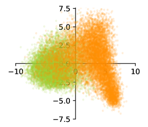
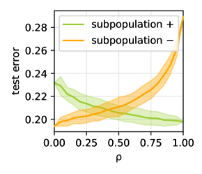
Figure A.1: Relative representation and bias. Numerical experiments on a sub-sample of the CelebA dataset. (Left) A 2D projection of the pre-processed dataset, obtained from PCA, where the colours represent the two sub-populations. (Right) Per community test error, as the fraction of samples from the two subpopulations is varied (dataset dimension is fixed).

We construct a dataset by sub-sampling CelebA and by preprocessing the selected images through an Xception network [55] trained on ImageNet [56]. As depicted in the scatter plot in Fig. A.1, the first two principal components of the obtained data clearly reveal a clustered structure. Many attributes contained in the metadata are highly correlated with the split into these two sub-populations. For example, in the figure we colour the points according to the attribute "Wearing_Lipstick". Now, suppose we are interested in predicting a different target attribute, which is not as easily determined by just looking at the group membership, e.g. "Wavy_Hair". What happens to the model accuracy if one alters the relative representation of the two groups, e.g. when one varies the fraction of points that belong to the orange group?

The right panel of Fig. A.1 shows the outcome of this experiment. As we can see from the plot, the fact that a group is under-represented induces a gap in the generalisation performance of the model when evaluated on the different sub-populations. The presence of a gap is a clear indicator of unfairness, induced by an implicit bias towards the over-represented group.

Many factors might play a role in determining and exacerbating this phenomenon. This is precisely why designing a general recipe for a fair / unbiased classifier is a very challenging, if solvable, problem. Some bias inducing factors are linked to the sampling quality of the dataset, as in the case of the overall number of datapoints and the balance between the sub-populations frequencies. Other factors are controlled by the different degree of variability in the input distributions of each group. In other cases the imbalance is hidden and can only be recognised by looking at the joint distribution of inputs and labels. For example, the balance between the positive/negative labels might differ among the groups and may be strongly correlated with the group membership. Even similar individuals with different group memberships might be labelled differently. The present work aims at modelling the data structure observed in these types of experiments, to obtain detailed understanding of the various sources of bias in these problems.

A.2 Additional details on the CelebA experiments

The CelebA dataset is a collection of $202.599$ face images of various celebrities, accompanied by $40$ binary attributes per image (for instance, whether a celebrity features black hairs or not) [16]. To obtain the results presented in the main text we apply the following pre-processing pipeline: We first downsample CelebA up to $20.000$ images. Notice that this is done with the purpose of considering settings with limited amount of available data. Indeed, as we have seen in the main manuscript, data scarcity is one of the main bias-inducing ingredients. We are thus not interested to consider the entire CelebA dataset, especially for simple classification tasks like the one described in the main text. By exploiting the deep learning framework provided by Tensorflow [58], we then pre-process the dataset using the features extracted from an Xception convolutional network [55] pre-trained on Imagenet [56]. Finally, we collect the extracted features together with the associated binary attributes in a json file.

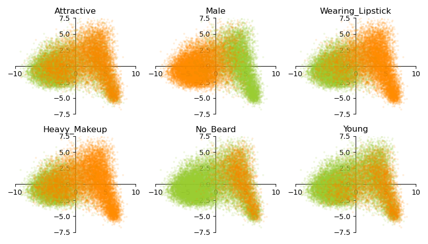
Figure A.2: Clustering CelebA according to attributes. We show 6 of the 40 attributes in CelebA demonstrating a neat clustering.

By applying PCA on the pre-processed dataset, we observe a clustering structure in the data when projected to the space of the PCA principal components. The clusters appear to reflect a natural correspondence with the binary attributes associated to each input data point, however this is not a general implication and many datasets show clustering with a non interpretable connection to the attributes. The clusters can be clearly seen in Fig. A.2, where we use colours to show whether a celebrity features a given attribute (green dots) or not (orange dots). In the plot, the axes correspond to the directions traced by the two PCA leading eigenvectors. As we can see from Fig. A.2, the two sub-populations are overlapping and hard to disentangle. This situation precisely corresponds to the high-noise regime the T-M model is meant to describe. Among the various clustering depicted in Fig. A.2, we decided to disregard those corresponding to ethically questionable attributes, such as "Attractive", "Male" or "Young". Finally, we chose as sensitive attribute – determining the membership in the subpopulations – the "Wearing_Lipstick" feature since it gives a more homogeneous distribution of the data points in the two clusters.

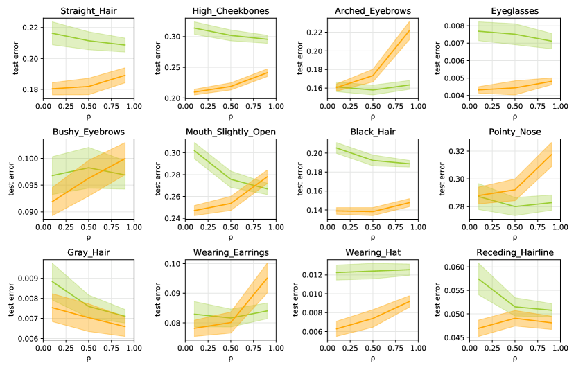
Figure A.3: Relative representation across attributes. The panels show the generalisation error depending on the relative representation in different attributes. The sub-populations $+$ (green) $-$ (orange) are obtained splitting according to the attribute "Wearing_Lipstick". The simulations are averaged over $100$ samples.

Anyone of the other attributes can be considered as a possible target, and thus be used to label the data points. The final pre-processing step consist in downsampling further the data in order to have the same ratio of $0$ and $1$ labels in the two subpopulations. This step helps mitigating bias induced by the different ratio of label in the two subpopulations and simplifies the identification of the other sources of bias. The general case can be addressed in the T-M model, in Sec. B we comment more on the bias induced by different label ratios.

As Fig. A.3 illustrates, there is a large number of possible outcomes concerning the behaviour of the test error as a function of the relative representation. Indeed, as we have seen in the main text, the presence and the position of the crossing point strictly depends on both the cluster variances and the amount of available data. Despite all these behaviours are fully reproducible in the T-M model by means of its corresponding parameters, we here decided to chose the “Wavy_Hair" as target feature because it shows a nicely symmetric profile of the test error that is more suitable for illustration purposes. To get the learning curves in Fig. A.3, we train a classifier with logistic regression and $L_{2}$-regularisation. In particular, we use the LogisticRegression class from scikit-learn [59]. This class implements several logistic regression solvers, among which the lbfgs optimizer. This solver implements a second order gradient descent optimization which can consistently speed-up the training process. The training algorithm stops either if the maximum component of the gradient goes below a certain threshold, or if a maximum number of iterations is reached. In our case, we set the threshold at $1e-15$ and the maximum number of iterations to $10^{5}$. The parameter penalty of the LogisticRegression class is a flag determining whether an $L_{2}$-regularisation needs to be added to the training or not. The C hyper-parameter corresponds instead to the inverse of the regularisation strength. In our experiments, we chose the value of the regularisation strength by cross-validation in the interval $(10^{-3},10^{3})$ with $30$ points sampled in logarithmic scale.

A.3 Other datasets

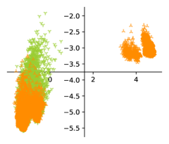
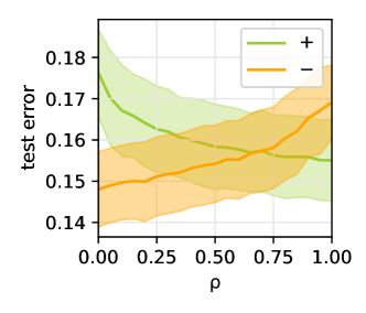
Figure A.4: MEPS dataset. (Left) Clustering in the MEPS dataset, according to be above or below the average age. (Right) Crossing of the generalisation error as the relative representation $\rho$ is changed. The simulations are averaged over $100$ samples.

The observations made on the CelebA dataset are quite general and can be further extended to lower-dimensional datasets. As example of this, we considered the Medical Expenditure Panel Survey (MEPS) dataset. This is a dataset containing a large set of surveys which have been conducted across the United States in order to quantify the cost and use of health care and health insurance coverage. The dataset consists of about $150$ features, including sensitive attributes, such as age or medical sex, as well as attributes describing the clinical status of each patient. The label is instead binary and measures the expenditure on medical services of each individual, assessing whether the total amount of medical expenses is below or above a certain threshold. As it can be seen in Fig. A.4, the behaviour is qualitatively similar to the one already observed in the CelebA dataset of celebrity face images. Indeed, even in this case, PCA shows the presence of two distinct clusters when considering the age as the sensitive attribute and then splitting the dataset in two sub-populations, according to the middle point of the age distribution. Moreover, the generalisation error per community exhibits a crossing according to the relative representation.

Appendix B Exploration of the parameter space

B.1 Supporting results

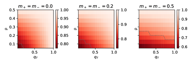
Figure B.1: Bias with two different rules to be learned. The three phase diagrams give the DI depending on $\rho$ (y-axis) and $q_{T}$ (x-axis). Moving from the left panel to the right panel $m_{+}$ and $m_{i}$ are increased. The other parameters are: $\alpha=0.5,\Delta_{+}=0.5,\Delta_{-}=0.5,b_{+}=0,b_{-}=0$.

This section presents supporting results on the sources of bias. In Fig. B.1, we re-propose the the study of the disparate impact (DI) depending on the relative representation $\rho$ and the rule similarity $q_{T}$, paying close attention to the role of the group-label correlation $m_{+}$, $m_{-}$. Interestingly, if $m_{+}=m_{-}=0$, when the rules become identical ($q_{T}=1$) the bias is removed. However if $m_{+}=m_{-}\neq 0$ this is no longer true. This shows once again that it is not sufficient for a classifier to be able of reproducing the rule, as bias can appear in reason of other concurring factors.

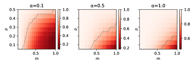
Figure B.2: Bias with a learnable rule. We show the accuracy gain as function of the proportion of group $+$ ($\rho$) and the correlation between label and group ($m_{+},m_{-}$). The different figures show how of increasing the dataset size (increasing from left to right) mitigates the bias. The other parameters are: $q_{T}=1.0,\Delta_{+}=0.5,\Delta_{-}=0.5,b_{+}=0,b_{-}=0$.

The main difference with respect to the case with $q_{T}\neq 1$ is that, if $q_{T}=1$, increasing the amount of training data can be a solution. In fact, bias at $q_{T}=1$ is due to overfitting with respect ot the largest sub-population, and this effect can be cured by increasing in $\alpha$. This is illustrated in Fig. B.2, that extends the figure of the main text showing the effect of $\alpha$. Moving from left to right, $\alpha$ increases and the area where the $80\%$ rule is violated shrinks down.

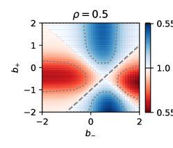
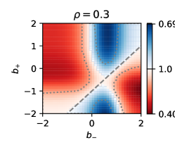
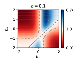
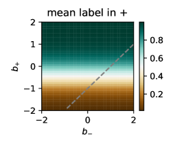
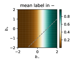
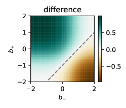
Figure B.3: Labels within groups and classifier bias. The first row shows the DI as faction of $b_{+}$ and $b_{-}$ with $\Delta_{+}=\Delta_{-}=0.5$, $\alpha=0.5$, $m_{+}=m_{-}=0.5$. From left to right, the relative representation $\rho$ moves from equally represented groups to having group $+$ under-represented. The 80% threshold is denoted by the dotted line. The dashed line indicates equal within-group label fraction. The second row shows the average labelling in $+$ (left), $-$ (centre), and their difference (right). Notice that these diagrams are independent of $\rho$ and therefor apply to the three settings shown in the first row.

The results shown until this point are agnostic with respect to the relative fraction of labels inside the sub-populations. When this quantity is strongly varied across the groups, it can contribute to an additional source of bias, especially if combined with a small relative representation. Indeed, the classifier can simply bias its prediction towards the most likely outcome reaching an accuracy that apparently exceeds random guessing, without effectively doing any informed prediction. Many factors play a role in deciding the relative fraction of labels in the T-M model, the bias terms ($b_{+}$ and $b_{-}$) are the most relevant since they directly shift the decision boundaries. We consider these two parameters in Fig. B.3 to exemplify this concept.

When the sub-populations are equally represented $\rho=0.5$, the separations between bias towards $+$ or $-$ is clearly marked by two straight lines. One separation is simply given by the line of equal label fraction, the other is given by the uncertainty of the classifier, receiving contrasting inputs from the two groups. As the relative representation $\rho$ decreases, the classifier accommodates the inputs from the largest group and the separation line is distorted. Finally, observe that the line of equal label fraction (bottom right panel) is not centred in the diagram because $m_{+}=m_{-}\neq 0$.

Appendix C Mitigation strategies

Real data.

In Fig. 3 of the main text, we show the effect of reweighing in the synthetic model. The same analysis can be applied to real data, yielding similar results. In particular, in line with the other validations, we present in Fig. C.1 the result for the CelebA dataset when the splitting is done according to the "Wearing_Lipstick" and the target feature is "Wavy_Hair".

Figure C.1: Mitigation using re-weighting on real data. The four panels show the same quantities as in Fig. 3A but applied to the CelebA dataset. Each panels shows in upper figure the mutual information on the fairness metrics – statistical parity, equal opportunities, equal accuracy, equal odds, predicted parity $1$, and predicted parity $10$– and in the lower figure the accuracy of for subpopulation $+$ and subpopulation $-$. The first 3 panels show the effect on the reweighing strategy for different values of the label weight (from left to right $w_{l}=0.1,0.5,0.9$). The last panel shows the performance of the coupled neural network strategy.

Similarly to what observa in the synthetic dataset, the coupled neural network strategy allows for a better performance on all the fairness metrics while retraining a high accuracy for both subpopulations.

Additional results varying group membership.

Some strategies require information concerning the group membership of each data point. Depending on the situation, this information may contain errors or it may even be unavailable. Consequently we should take into account the robustness of the mitigation strategies with respect to these errors. Call $\eta$ the fraction of points for which the group was correctly assessed. The phase diagrams in Fig. C.2a show the DI under the reweighing mitigation scheme (controlling the group importance in the loss) and the coupled classifier mitigation. We can clearly observe a greater resilience to the error rates in the case of our strategy. The reweighing strategy appears to have low DI only in extreme cases, where the accuracy on the largest sub-population is greatly deteriorated.

We can understand the larger picture by looking at the different fairness metrics described in the main text, Fig. C.2b, for which the same observations apply. Since $\eta$ is not an actual hyper-parameter, but rather represents an imperfect imputation of the group structure, we consider the maximum for each value of $\eta$. The picture seems quite robust on the side of reweighing (upper group): for every $\eta$ the maximum is achieved for different values of the parameters. Instead, the picture changes for the coupled classifiers (lower group): the method is robust to this perturbation until a critical value (roughly 25% of mismatched inputs), where the minima of the MI become inconsistent and therefore the fairness metrics cannot be optimised all at once.

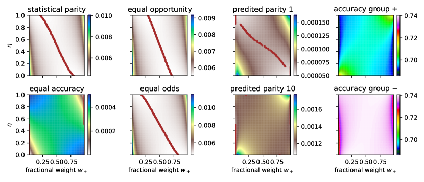
(a) MI with errors in the group membership under community re-weighting strategy.

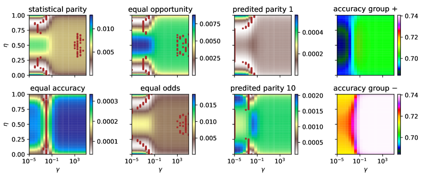
(b) MI with errors in the group membership under coupled neural networks strategy.

Figure C.2: Effect of noise in the attribute of the sub-communities. In the heatmaps we show in colors how having imperfect information concerning the sub-community membership affect each fairness metrics (six left figures) and the accuracy (right two plots). The vertical axis of the figures represents the probability of mismatch $\eta$, while the horizontal axis refer to the parameter of the strategy ($w_{+}$ and $\gamma$ resepctively). For every value of the mismatch probability, we denote with red points the minima of the mutual information for each fairness metrics.

References

- [1] Joy Buolamwini and Timnit Gebru. Gender shades: Intersectional accuracy disparities in commercial gender classification. In Conference on fairness, accountability and transparency, pages 77–91. PMLR, 2018.
- [2] Laura Weidinger, John Mellor, Maribeth Rauh, Conor Griffin, Jonathan Uesato, Po-Sen Huang, Myra Cheng, Mia Glaese, Borja Balle, Atoosa Kasirzadeh, et al. Ethical and social risks of harm from language models. arXiv preprint arXiv:2112.04359, 2021.
- [3] Ruha Benjamin. Race after technology: Abolitionist tools for the new jim code. Social Forces, 2019.
- [4] Safiya Umoja Noble. Algorithms of oppression. New York University Press, 2018.
- [5] Virginia Eubanks. Automating inequality: How high-tech tools profile, police, and punish the poor. St. Martin’s Press, 2018.
- [6] Meredith Broussard. Artificial unintelligence: How computers misunderstand the world. mit Press, 2018.
- [7] Harini Suresh and John Guttag. Understanding potential sources of harm throughout the machine learning life cycle. 2021.
- [8] Caroline Criado Perez. Invisible women: Data bias in a world designed for men. Abrams, 2019.
- [9] Sotiris Kotsiantis, Dimitris Kanellopoulos, Panayiotis Pintelas, et al. Handling imbalanced datasets: A review. GESTS international transactions on computer science and engineering, 30(1):25–36, 2006.
- [10] Le Wang, Meng Han, Xiaojuan Li, Ni Zhang, and Haodong Cheng. Review of classification methods on unbalanced data sets. IEEE Access, 9:64606–64628, 2021.
- [11] Xue-wen Chen and Michael Wasikowski. Fast: a roc-based feature selection metric for small samples and imbalanced data classification problems. In Proceedings of the 14th ACM SIGKDD international conference on Knowledge discovery and data mining, pages 124–132, 2008.
- [12] Nitesh V Chawla, Kevin W Bowyer, Lawrence O Hall, and W Philip Kegelmeyer. Smote: synthetic minority over-sampling technique. Journal of artificial intelligence research, 16:321–357, 2002.
- [13] Xu-Ying Liu, Jianxin Wu, and Zhi-Hua Zhou. Exploratory undersampling for class-imbalance learning. IEEE Transactions on Systems, Man, and Cybernetics, Part B (Cybernetics), 39(2):539–550, 2008.
- [14] Zeyu Wang, Klint Qinami, Ioannis Christos Karakozis, Kyle Genova, Prem Nair, Kenji Hata, and Olga Russakovsky. Towards fairness in visual recognition: Effective strategies for bias mitigation. In Proceedings of the IEEE/CVF conference on computer vision and pattern recognition, pages 8919–8928, 2020.
- [15] Badr Youbi Idrissi, Martin Arjovsky, Mohammad Pezeshki, and David Lopez-Paz. Simple data balancing achieves competitive worst-group-accuracy. In Conference on Causal Learning and Reasoning, pages 336–351. PMLR, 2022.
- [16] Ziwei Liu, Ping Luo, Xiaogang Wang, and Xiaoou Tang. Deep learning face attributes in the wild. In Proceedings of International Conference on Computer Vision (ICCV), December 2015.
- [17] Robert N Hughes. Sex does matter: comments on the prevalence of male-only investigations of drug effects on rodent behaviour. Behavioural pharmacology, 18(7):583–589, 2007.
- [18] Robert N Hughes. Sex still matters: has the prevalence of male-only studies of drug effects on rodent behaviour changed during the past decade? Behavioural pharmacology, 30(1):95–99, 2019.
- [19] Lenka Zdeborová and Florent Krzakala. Statistical physics of inference: Thresholds and algorithms. Advances in Physics, 65(5):453–552, 2016.
- [20] Francesca Mignacco, Florent Krzakala, Yue Lu, Pierfrancesco Urbani, and Lenka Zdeborova. The role of regularization in classification of high-dimensional noisy gaussian mixture. In International Conference on Machine Learning, pages 6874–6883. PMLR, 2020.
- [21] Luca Saglietti and Lenka Zdeborová. Solvable model for inheriting the regularization through knowledge distillation. In Mathematical and Scientific Machine Learning, pages 809–846. PMLR, 2022.
- [22] Michael Feldman, Sorelle A Friedler, John Moeller, Carlos Scheidegger, and Suresh Venkatasubramanian. Certifying and removing disparate impact. In proceedings of the 21th ACM SIGKDD international conference on knowledge discovery and data mining, pages 259–268, 2015.
- [23] US Equal Employment Opportunity Commission et al. Questions and answers to clarify and provide a common interpretation of the uniform guidelines on employee selection procedures. US Equal Employment Opportunity Commission: Washington, DC, USA, 1979.
- [24] Patrick Charbonneau, Enzo Marinari, Marc Mézard, Giorgio Parisi, Federico Ricci-Tersenghi, Gabriele Sicuro, and Francesco Zamponi. Spin Glass Theory and Far Beyond. WORLD SCIENTIFIC, 2023.
- [25] Marc Mézard, Giorgio Parisi, and Miguel Angel Virasoro. Spin glass theory and beyond: An Introduction to the Replica Method and Its Applications, volume 9. World Scientific Publishing Company, 1987.
- [26] Andreas Engel and Christian Van den Broeck. Statistical mechanics of learning. Cambridge University Press, 2001.
- [27] Christos Thrampoulidis, Samet Oymak, and Babak Hassibi. Regularized linear regression: A precise analysis of the estimation error. In Conference on Learning Theory, pages 1683–1709. PMLR, 2015.
- [28] Bruno Loureiro, Cedric Gerbelot, Hugo Cui, Sebastian Goldt, Florent Krzakala, Marc Mezard, and Lenka Zdeborová. Learning curves of generic features maps for realistic datasets with a teacher-student model. Advances in Neural Information Processing Systems, 34:18137–18151, 2021.
- [29] Cynthia Dwork, Moritz Hardt, Toniann Pitassi, Omer Reingold, and Richard Zemel. Fairness through awareness. In Proceedings of the 3rd innovations in theoretical computer science conference, pages 214–226, 2012.
- [30] Jon Kleinberg, Sendhil Mullainathan, and Manish Raghavan. Inherent trade-offs in the fair determination of risk scores. arXiv preprint arXiv:1609.05807, 2016.
- [31] Sam Corbett-Davies, Emma Pierson, Avi Feller, Sharad Goel, and Aziz Huq. Algorithmic decision making and the cost of fairness. In Proceedings of the 23rd acm sigkdd international conference on knowledge discovery and data mining, pages 797–806, 2017.
- [32] Moritz Hardt, Eric Price, and Nati Srebro. Equality of opportunity in supervised learning. Advances in neural information processing systems, 29, 2016.
- [33] Muhammad Bilal Zafar, Isabel Valera, Manuel Gomez Rogriguez, and Krishna P Gummadi. Fairness constraints: Mechanisms for fair classification. In Artificial Intelligence and Statistics, pages 962–970. PMLR, 2017.
- [34] Alexandra Chouldechova. Fair prediction with disparate impact: A study of bias in recidivism prediction instruments. Big data, 5(2):153–163, 2017.
- [35] Federica Gerace, Luca Saglietti, Stefano Sarao Mannelli, Andrew Saxe, and Lenka Zdeborová. Probing transfer learning with a model of synthetic correlated datasets. Machine Learning: Science and Technology, 2022.
- [36] Till Speicher, Hoda Heidari, Nina Grgic-Hlaca, Krishna P Gummadi, Adish Singla, Adrian Weller, and Muhammad Bilal Zafar. A unified approach to quantifying algorithmic unfairness: Measuring individual &group unfairness via inequality indices. In Proceedings of the 24th ACM SIGKDD International Conference on Knowledge Discovery & Data Mining, pages 2239–2248, 2018.
- [37] Alessandro Castelnovo, Riccardo Crupi, Greta Greco, Daniele Regoli, Ilaria Giuseppina Penco, and Andrea Claudio Cosentini. A clarification of the nuances in the fairness metrics landscape. Scientific Reports, 12(1):1–21, 2022.
- [38] Alekh Agarwal, Alina Beygelzimer, Miroslav Dudík, John Langford, and Hanna Wallach. A reductions approach to fair classification. In International Conference on Machine Learning, pages 60–69. PMLR, 2018.
- [39] Alekh Agarwal, Miroslav Dudík, and Zhiwei Steven Wu. Fair regression: Quantitative definitions and reduction-based algorithms. In International Conference on Machine Learning, pages 120–129. PMLR, 2019.
- [40] L Elisa Celis, Lingxiao Huang, Vijay Keswani, and Nisheeth K Vishnoi. Classification with fairness constraints: A meta-algorithm with provable guarantees. In Proceedings of the conference on fairness, accountability, and transparency, pages 319–328, 2019.
- [41] Sam Corbett-Davies and Sharad Goel. The measure and mismeasure of fairness: A critical review of fair machine learning. arXiv preprint arXiv:1808.00023, 2018.
- [42] Solon Barocas, Moritz Hardt, and Arvind Narayanan. Fairness and Machine Learning. fairmlbook.org, 2019. http://www.fairmlbook.org.
- [43] Faisal Kamiran and Toon Calders. Data preprocessing techniques for classification without discrimination. Knowledge and information systems, 33(1):1–33, 2012.
- [44] Drago Plecko and Nicolai Meinshausen. Fair data adaptation with quantile preservation. Journal of Machine Learning Research, 21(242):1–44, 2020.
- [45] Kristian Lum and James Johndrow. A statistical framework for fair predictive algorithms. arXiv preprint arXiv:1610.08077, 2016.
- [46] Andrei A Rusu, Neil C Rabinowitz, Guillaume Desjardins, Hubert Soyer, James Kirkpatrick, Koray Kavukcuoglu, Razvan Pascanu, and Raia Hadsell. Progressive neural networks. arXiv preprint arXiv:1606.04671, 2016.
- [47] Friedemann Zenke, Ben Poole, and Surya Ganguli. Continual learning through synaptic intelligence. In International Conference on Machine Learning, pages 3987–3995. PMLR, 2017.
- [48] Luca Saglietti, Stefano Sarao Mannelli, and Andrew Saxe. An analytical theory of curriculum learning in teacher-student networks. arXiv preprint arXiv:2106.08068, 2021.
- [49] Toon Calders and Sicco Verwer. Three naive bayes approaches for discrimination-free classification. Data mining and knowledge discovery, 21(2):277–292, 2010.
- [50] Sanghamitra Dutta, Dennis Wei, Hazar Yueksel, Pin-Yu Chen, Sijia Liu, and Kush Varshney. Is there a trade-off between fairness and accuracy? a perspective using mismatched hypothesis testing. In International conference on machine learning, pages 2803–2813. PMLR, 2020.
- [51] Elisabetta Cornacchia, Francesca Mignacco, Rodrigo Veiga, Cédric Gerbelot, Bruno Loureiro, and Lenka Zdeborová. Learning curves for the multi-class teacher–student perceptron. Machine Learning: Science and Technology, 4(1):015019, 2023.
- [52] Shiori Sagawa, Aditi Raghunathan, Pang Wei Koh, and Percy Liang. An investigation of why overparameterization exacerbates spurious correlations. In International Conference on Machine Learning, pages 8346–8356. PMLR, 2020.
- [53] Samuel James Bell and Levent Sagun. Simplicity bias leads to amplified performance disparities. In Proceedings of the 2023 ACM Conference on Fairness, Accountability, and Transparency, pages 355–369, 2023.
- [54] Lynn A. Blewett, Julia A. Rivera Drew, Risa Griffin, Natalie Del Ponte, and Pat Convey. IPUMS health surveys: Medical expenditure panel survey, version 2.1 [dataset]. Minneapolis, MN: IPUMS, 2021.
- [55] François Chollet. Xception: Deep learning with depthwise separable convolutions. In Proceedings of the IEEE conference on computer vision and pattern recognition, pages 1251–1258, 2017.
- [56] Jia Deng, Wei Dong, Richard Socher, Li-Jia Li, Kai Li, and Li Fei-Fei. Imagenet: A large-scale hierarchical image database. In 2009 IEEE conference on computer vision and pattern recognition, pages 248–255. Ieee, 2009.
- [57] Emily Denton, Ben Hutchinson, Margaret Mitchell, and Timnit Gebru. Detecting bias with generative counterfactual face attribute augmentation. 2019.
- [58] Martín Abadi, Ashish Agarwal, Paul Barham, Eugene Brevdo, Zhifeng Chen, Craig Citro, Greg S. Corrado, Andy Davis, Jeffrey Dean, Matthieu Devin, Sanjay Ghemawat, Ian Goodfellow, Andrew Harp, Geoffrey Irving, Michael Isard, Yangqing Jia, Rafal Jozefowicz, Lukasz Kaiser, Manjunath Kudlur, Josh Levenberg, Dandelion Mané, Rajat Monga, Sherry Moore, Derek Murray, Chris Olah, Mike Schuster, Jonathon Shlens, Benoit Steiner, Ilya Sutskever, Kunal Talwar, Paul Tucker, Vincent Vanhoucke, Vijay Vasudevan, Fernanda Viégas, Oriol Vinyals, Pete Warden, Martin Wattenberg, Martin Wicke, Yuan Yu, and Xiaoqiang Zheng. TensorFlow: Large-scale machine learning on heterogeneous systems, 2015. Software available from tensorflow.org.
- [59] F. Pedregosa, G. Varoquaux, A. Gramfort, V. Michel, B. Thirion, O. Grisel, M. Blondel, P. Prettenhofer, R. Weiss, V. Dubourg, J. Vanderplas, A. Passos, D. Cournapeau, M. Brucher, M. Perrot, and E. Duchesnay. Scikit-learn: Machine learning in Python. Journal of Machine Learning Research, 12:2825–2830, 2011.