A parton branching with transverse momentum dependent splitting functions

Abstract

Off-shell, transverse-momentum dependent splitting functions can be defined from the high-energy limit of partonic decay amplitudes. Based on these splitting functions, we construct Sudakov form factors and formulate a new parton branching algorithm. We present a first Monte Carlo implementation of the algorithm. We use the numerical results to verify explicitly momentum sum rules for TMD parton distributions.

CERN-TH-2022-087
                                                                                                                     IFJPAN-IV-2022-8

Experimental analyses in high-energy physics depend on event simulations performed through Monte Carlo (MC) generators [1] based on parton branching methods. The development of MC event generators is crucial for the planning of future experimental programs such as the High-Luminosity Large Hadron Collider (HL-LHC) [2], the proposed forward physics facility [3] and hadron-electron facility [4] at the HL-LHC, the Electron Ion Collider (EIC) [5] and the Future Circular Collider (FCC) [6].

While most MC tools rely on the description of hadron structure provided by collinear parton distribution functions (PDFs) [7], ongoing advances in MC generators raise the question of assessing the impact of a more complete description of hadron structure including transverse momentum dependent (TMD) parton distributions [8] on MC simulations. In fact, several developments of the last few years in parton branching methods have involved aspects of TMD physics. This includes, for instance, TMD perturbative resummation and its matching with finite-order next-to-next-to-leading (NNLO) corrections [9, 10]; parton branching formulation of the evolution of TMD distributions [11, 12]; implementation of soft and collinear corrections in parton showers with subleading-logarithmic accuracy [13, 14]; multi-jet merging with TMD parton showers [15, 16].

In this work we begin an investigation of the transverse momentum dependence at the level of the partonic splitting functions [17, 18, 19], an aspect which has not been explored so far in parton branching MC. To this end we propose using off-shell TMD splitting functions defined from the high-energy limit of QCD multi-parton amplitudes according to the high-energy factorization method [20]. We construct a parton branching formalism based on the TMD splitting functions thus defined.

To do this, we employ the approach [11, 12] and extend it to introduce new real-emission TMD splitting kernels and new Sudakov form factors. This approach makes use of the concept of “unitarity”, commonly applied in parton-showering algorithms, to relate real and virtual emissions, and to express Sudakov form factors in terms of real-emission kernels and soft-gluon resolution scales. In this respect it differs from the treatment of Sudakov factors in terms of integrals over virtual emissions, used in several computations based on TMD dynamics, e.g. [21, 22] and [23, 24]. The approach we use is well-suited for the implementation of the transverse momentum dependence in real-emission kernels, exploiting the positivity of the splitting function defined through the method [20]. Since the splitting function [20], once combined with factorization formulas in transverse momentum, accomplishes the small-$x$ resummation in the evolution kernels [25], this study constitutes a first step toward a full generator extending [11, 12] to the small-$x$ phase space [26]. In this Letter we present the branching evolution equations which result from this approach, and illustrate two numerical applications to the momentum sum rule and to the evolution of TMD parton distributions. An earlier discussion of results from this investigation may be found in [27].

We will proceed as follows. We will first briefly discuss the TMD splitting functions. Next we will describe their parton branching implementation. We will finally present MC results from the numerical solution of the branching equations.

Consider the initial-state (spacelike) parton cascade in Fig. 1. We use a Sudakov parameterization of the four-momenta along the decay chain in terms of lightcone and transverse momenta. For the gluon to quark splitting process depicted in Fig. 1 we parameterize the four-momenta $k$ and $k^{\prime}$ as

$$k=xp+k_{T}+{{k^{2}+{k}_{\perp}^{2}}\over{2xp\cdot{\overline{p}}}}\ {\overline{p}}\;\;\;,\;\;\;\;\;k^{\prime}=x^{\prime}p+k_{T}^{\prime}+{{k^{\prime 2}+{k}_{\perp}^{\prime 2}}\over{2x^{\prime}p\cdot{\overline{p}}}}\ {\overline{p}}\;.$$ (1)

Here we use the notation $v^{\mu}=(v^{+},v^{-},{v}_{\perp})$ for any four-vector, with $v^{\pm}=(v^{0}\pm v^{3})/\sqrt{2}$ lightcone components and ${v}_{\perp}$ two-dimensional euclidean vector; the reference (lightcone) momenta $p$ and ${\overline{p}}$ are $p=(\sqrt{s/2},0,0_{\perp})$, ${\overline{p}}=(0,\sqrt{s/2},0_{\perp})$; the transverse momenta fulfill $k_{T}^{2}=-k_{\perp}^{2}$, $k_{T}^{\prime 2}=-k_{\perp}^{\prime 2}$. We define the lightcone momentum transfer at the splitting as $z=x/x^{\prime}$. By four-momentum conservation, we have

$$k^{\prime 2}={q^{2}\over{1-z}}+{k^{2}\over z}+{{\tilde{q}}_{\perp}^{2}\over{z(1-z)}}\;,$$ (2)

where ${\tilde{q}}_{\perp}=k_{\perp}-zk_{\perp}^{\prime}$.

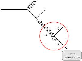
Figure 1: Spacelike parton cascade.

The splitting probability for the off-shell gluon to quark splitting process in Fig. 1 can be defined and computed by high-energy factorization [20] as a function of the strong coupling $\alpha_{s}$, lightcone momentum transfer $z$, and transverse momenta $k_{\perp}^{\prime}$ and ${\tilde{q}}_{\perp}$. Its explicit expression is given by

$${P}_{qg}\left(\alpha_{s},z,{k_{\perp}^{\prime}},{\tilde{q}}_{\perp}\right)={{\alpha_{s}T_{F}}\over{2\pi}}{{{\tilde{q}}_{\perp}^{2}z(1-z)}\over{({\tilde{q}}_{\perp}^{2}+z(1-z){k}_{\perp}^{\prime 2})^{2}}}\left[{{{\tilde{q}}_{\perp}^{2}}\over{z(1-z)}}+4(1-2z){\tilde{q}}_{\perp}\cdot{k}_{\perp}^{\prime}-4{{({\tilde{q}}_{\perp}\cdot{k_{\perp}^{\prime}})^{2}}\over{{k}_{\perp}^{\prime 2}}}+4z(1-z){k}_{\perp}^{\prime 2}\right],$$ (3)

where $T_{F}$ is the color trace invariant, $T_{F}=1/2$. For $k_{\perp}^{\prime 2}\ll k_{\perp}^{2}$, after angular average the TMD splitting probability in Eq. (3) returns, for all lightcone momentum fractions $z$, the leading-order collinear splitting function [28, 29, 30]. For finite $k_{\perp}^{\prime 2}$ such that $k_{\perp}^{\prime 2}\sim{\cal O}(k_{\perp}^{2})$, on the other hand, Eq. (3) gives a series expansion in powers $({k_{\perp}^{\prime 2}}/{{\tilde{q}}_{\perp}^{2}})^{n}$, with $z$-dependent coefficients. These finite-$k_{\perp}^{\prime 2}$ contributions, through convolution with transverse momentum dependent gluon Green’s functions [20, 31, 32], provide the resummation of the higher-order corrections to the gluon to quark splitting function that are logarithmically enhanced for $z\to 0$ [25], at all orders in $\alpha_{s}$. Off-shell TMD splitting functions obtained by high-energy factorization have been further studied in the context of forward Drell-Yan production in [33], and have been computed for all partonic channels in [34, 35, 36]. These splitting functions are positive definite and interpolate consistently between the collinear limit and the high-energy limit [20, 34, 36].

To construct a parton branching based on TMD splitting functions, we extend the method [12]. We introduce the soft-gluon resolution scale $z_{M}$ to separate resolvable and non-resolvable branchings, and consider the branching evolution of the momentum weighted TMD parton distributions $\tilde{\mathcal{A}}_{a}(x,k_{\perp}^{2},\mu^{2})$, where $a$ is the flavor index, $x$ is the longitudinal momentum fraction, $k_{\perp}$ is the transverse momentum, and $\mu$ is the evolution variable. We require that the resolvable branchings are described by emission kernels given by the TMD splitting functions. Based on the behavior of TMD distributions with respect to the resolution scale $z_{M}$ analyzed in [11, 37], we also require the evolution to be angular-ordered. For the evolution of $\tilde{\mathcal{A}}_{a}$ from scale $\mu_{0}$ to scale $\mu$ we write

$$\tilde{\mathcal{A}}_{a}(x,k_{\perp}^{2},\mu^{2}) =\tilde{\mathcal{A}}_{a}(x,k_{\perp}^{2},\mu_{0}^{2})-\int{{d^{2}\mu_{\perp}^{\prime}}\over{\pi\mu_{\perp}^{\prime 2}}}F_{a}(\mu_{\perp}^{\prime 2},k_{\perp}^{2})\tilde{\mathcal{A}}_{a}(x,k_{\perp}^{2},\mu_{\perp}^{\prime 2})\Theta(\mu_{\perp}^{\prime 2}-\mu_{0}^{2})\Theta(\mu^{2}-\mu_{\perp}^{\prime 2})+$$

$$+\sum_{b}\int{{d^{2}\mu_{\perp}^{\prime}}\over{\pi\mu_{\perp}^{\prime 2}}}\int\limits_{x}^{z_{M}}dz\tilde{P}^{R}_{ab}(z,k_{\perp}+(1-z)\mu_{\perp}^{\prime},\mu_{\perp}^{\prime})\tilde{\mathcal{A}}_{b}\left({{x}\over{z}},(k_{\perp}+(1-z)\mu_{\perp}^{\prime})^{2},\mu^{\prime 2}\right)\Theta(\mu_{\perp}^{\prime 2}-\mu_{0}^{2})\Theta(\mu^{2}-\mu_{\perp}^{\prime 2}),$$ (4)

where the virtual corrections and non-resolvable branchings are collectively represented by the contribution in $F_{a}$ in the first line, in which $F_{a}$ is a kernel to be determined, and the resolvable branchings are described by the term in the second line through the TMD, fully angle-dependent splitting functions $\tilde{P}^{R}_{ab}$. The explicit expressions for the functions $\tilde{P}^{R}_{ab}$ are given in [20, 33, 34, 35, 36].

To determine the specific form of $F_{a}$, we apply the “unitarity” approach, analogously to [12]. Using four-momentum conservation, we require that the sum over flavors of the normalization integrals for TMD distributions $\tilde{\mathcal{A}}_{a}$ is not changed by evolution, so that

$$0=\sum_{a}\int_{0}^{1}dx\int dk_{\perp}^{2}\tilde{\mathcal{A}}_{a}(x,k_{\perp}^{2},\mu^{2})-\sum_{a}\int_{0}^{1}dx\int dk_{\perp}^{2}\tilde{\mathcal{A}}_{a}(x,k_{\perp}^{2},\mu_{0}^{2}).$$ (5)

Inserting now the TMD PDF at the scale $\mu$ in the above relation, using Eq. (A parton branching with transverse momentum dependent splitting functions) and subsequently substituting $k_{\perp}^{\prime}=k_{\perp}+(1-z)\mu_{\perp}$ as well as $t=x/z$, the momentum sum rule yields the following relation between the real splitting functions and the non-resolvable branchings:

$$0=\sum_{b}\int{{d^{2}\mu_{\perp}^{\prime}}\over{\pi\mu_{\perp}^{\prime 2}}}\Theta(\mu_{\perp}^{\prime 2}-\mu_{0}^{2})\Theta(\mu^{2}-\mu_{\perp}^{\prime 2})\int\limits_{0}^{1}dt\int dk_{\bot}^{\prime 2}\left(F_{b}(\mu_{\perp}^{\prime 2},k_{\perp}^{\prime 2})-\sum_{a}\int\limits_{0}^{z_{M}}dz\ z\tilde{P}^{R}_{ab}(z,k_{\perp}^{\prime},\mu_{\perp}^{\prime})\right)\tilde{\mathcal{A}}_{b}(t,k_{\perp}^{\prime 2},\mu_{\perp}^{\prime 2}).$$ (6)

Therefore the sum rule allows us to fix the still missing term corresponding to non-resolvable branchings. Introducing the angular averaged TMD splitting functions $\bar{P}^{R}_{ba}(z,k_{\perp}^{2},\mu^{\prime 2})$, we have

$$F_{a}(\mu^{\prime 2},k_{\perp}^{2})=\sum_{b}\int\limits_{0}^{z_{M}}dz\ z\bar{P}^{R}_{ba}(z,k_{\perp}^{2},\mu^{\prime 2}).$$ (7)

With that we write Eq. (A parton branching with transverse momentum dependent splitting functions) in differential form,

$${{d\tilde{\mathcal{A}}_{a}(x,k_{\perp}^{2},\mu^{2})}\over{d\ln\mu^{2}}} =-\tilde{\mathcal{A}}_{a}(x,k_{\perp}^{2},\mu^{2})\sum_{b}\int_{0}^{z_{M}}dz\ z\bar{P}^{R}_{ba}(z,k_{\perp}^{2},\mu^{2})$$

$$+\sum_{b}\int{{d^{2}\mu_{\perp}^{\prime}}\over{\pi}}\delta(\mu^{2}-\mu_{\perp}^{\prime 2})\int\limits_{x}^{z_{M}}dz\tilde{P}^{R}_{ab}(z,k_{\perp}+(1-z)\mu_{\perp}^{\prime},\mu_{\perp}^{\prime})\tilde{\mathcal{A}}_{b}\left({{x}\over{z}},(k_{\perp}+(1-z)\mu_{\perp}^{\prime})^{2},\mu^{2}\right),$$ (8)

and introduce the TMD Sudakov form factor,

$$\Delta_{a}(\mu^{2},\mu_{0}^{2},k_{\perp}^{2})\equiv\Delta_{a}(\mu^{2},k_{\perp}^{2})=\exp\left(-\sum_{b}\int_{\mu_{0}^{2}}^{\mu^{2}}{{d\mu^{\prime 2}}\over{\mu^{\prime 2}}}\int_{0}^{z_{M}}dz\ z\bar{P}^{R}_{ba}(z,k_{\perp}^{2},\mu^{\prime 2})\right).$$ (9)

Using

$${{d\Delta_{a}(\mu^{2},k_{\perp}^{2})}\over{d\ln\mu^{2}}}=-\Delta_{a}(\mu^{2},k_{\perp}^{2})\sum_{b}\int_{0}^{z_{M}}dz\ z\bar{P}^{R}_{ba}(z,k_{\perp}^{2},\mu^{2}),$$ (10)

we arrive at

$${{d\tilde{\mathcal{A}}_{a}(x,k_{\perp}^{2},\mu^{2})}\over{d\ln\mu^{2}}} ={{1}\over{\Delta_{a}(\mu^{2},k_{\perp}^{2})}}{{d\Delta_{a}(\mu^{2},k_{\perp}^{2})}\over{d\ln\mu^{2}}}\tilde{\mathcal{A}}_{a}(x,k_{\perp}^{2},\mu^{2})$$

$$+\sum_{b}\int{{d^{2}\mu_{\perp}^{\prime}}\over{\pi}}\delta(\mu^{2}-\mu_{\perp}^{\prime 2})\int\limits_{x}^{z_{M}}dz\tilde{P}^{R}_{ab}(z,k_{\perp}+(1-z)\mu_{\perp}^{\prime},\mu_{\perp}^{\prime})\tilde{\mathcal{A}}_{b}\left({{x}\over{z}},(k_{\perp}+(1-z)\mu_{\perp}^{\prime})^{2},\mu^{2}\right).$$ (11)

By dividing Eq. (11) by $\Delta_{a}(\mu^{2},k_{\perp}^{2})$ and integrating over $d\ln\mu^{2}$, we obtain

$$\tilde{\mathcal{A}}_{a}\left(x,k_{\perp}^{2},\mu^{2}\right) =\Delta_{a}\left(\mu^{2},k_{\perp}^{2}\right)\tilde{\mathcal{A}}_{a}\left(x,k_{\perp}^{2},\mu_{0}^{2}\right)+$$

$$\sum_{b}\int{{d^{2}\mu_{\perp}^{\prime}}\over{\pi\mu_{\perp}^{\prime 2}}}\Theta(\mu_{\perp}^{\prime 2}-\mu_{0}^{2})\Theta(\mu^{2}-\mu_{\perp}^{\prime 2})\int\limits_{x}^{z_{M}}\textrm{d}z\,{{\Delta_{a}\left(\mu^{2},k_{\perp}^{2}\right)}\over{\Delta_{a}\left(\mu_{\perp}^{\prime 2},k_{\perp}^{2}\right)}}\tilde{P}_{ab}^{R}\left(z,k_{\perp}+(1-z)\mu_{\perp}^{\prime},\mu_{\perp}^{\prime}\right)\tilde{\mathcal{A}}_{b}\left({{x}\over{z}},(k_{\perp}+(1-z)\mu_{\perp}^{\prime})^{2},\mu_{\perp}^{\prime 2}\right).$$ (12)

The evolution equation (12) implies the introduction of the new Sudakov form factor defined in Eq. (9) in terms of angular-averaged TMD splitting functions. This is one of the main results of this paper. It can be compared with recent approaches [38, 39, 40, 41] aiming at a combined treatment of Sudakov and small-$x$ contributions to parton evolution. The distinctive feature of the approach presented in this paper is that the treatment is done at the level of unintegrated, $k_{\perp}$-dependent splitting functions which factorize in the high-energy limit and control the summation of small-$x$ logarithmic contributions to the evolution. These splitting functions are then used in the branching algorithm, where they are integrated to construct the new Sudakov factors. In what follows we present a numerical MC implementation of the Sudakov factor and evolution equation, and use the MC results to illustrate properties of the new algorithm.

To solve the new branching equation by the MC method, we note that all TMD splitting functions are positive definite, so that the procedure [12] applies. Compared to [12] we however adapt the implementation of the Sudakov form factor, to take account of the $k_{\bot}$-dependence, by making use of the veto algorithm [42]. In the MC code, the scale of the next branching $\mu_{i}$ is generated according to the Sudakov form factor,

$$R=1-{{\Delta_{a}(\mu_{i}^{2})}\over{\Delta_{a}(\mu_{i-1}^{2})}}\Leftrightarrow\mu_{i}^{2}=\Delta_{a}^{-1}((1-R)\Delta_{a}(\mu_{i-1}^{2})),$$ (13)

where R represents a uniformly distributed random number between zero and one. To find the inverse of the Sudakov form factor and generate $\mu_{i}$, in the case of collinear splitting functions a table of Sudakov factors is computed and interpolation methods are used to calculate $\mu_{i}$. In the case of the $k_{\bot}$-dependent Sudakov form factor, instead of extending the Sudakov table by an additional dimension we use the veto algorithm. By writing $\Delta_{a}(\mu^{2},k_{\bot}^{2})=\exp\left(-\int_{\mu_{0}^{2}}^{\mu^{2}}({d\mu^{\prime 2}}/{\mu^{\prime 2}})g_{a}(\mu^{\prime 2},k_{\bot}^{2})\right)$, with $g_{a}(\mu^{2},k_{\bot}^{2})=\sum_{b}\int_{0}^{z_{M}}dz\ z\ \bar{P}^{R}_{ba}(z,k_{\bot}^{2},\mu^{\prime 2})$ the differential branching probability, in the veto algorithm one proposes to find a function $g_{a}^{\prime}$ such that $g_{a}^{\prime}(\mu^{2})\geq g_{a}(\mu^{2},k_{\bot}^{2})$ for all $\mu$ and $k_{\bot}$ and proceeds in the following way:

1. start with $j=0$, $p_{j=0}^{2}=\mu_{i-1}^{2}$,

2. add one to j. Select $p^{2}_{j}>p^{2}_{j-1}$ according to $R=1-\exp\left(-\int_{p_{j-1}^{2}}^{p_{j}^{2}}({dp^{\prime 2}}/{p^{\prime 2}})g_{a}^{\prime}(p^{\prime 2})\right)$,

3. if $g(p^{2}_{j})/g^{\prime}(p^{2}_{j})\leq(\rm{newly\;generated})\;R$ go to 2,

4. else: $\mu_{i}^{2}=p^{2}_{j}$ is the generated scale.

The function $g^{\prime}$ is usually chosen to have a known inverse function, but for our application we choose $g_{a}^{\prime}(\mu^{2})=\sum_{b}\int_{0}^{z_{M}}dz\ z\ (P^{R}_{ba}(z)+h_{ba}(z))$, where the first term is the integral of the collinear splitting function and the function $h_{ba}$ is added to ensure that $g^{\prime}$ is larger than $g$ for all values of $k_{\bot}$ and $\mu$. This function $g^{\prime}$ does not have a known inverse, but has one variable less than the function $g$ (no $k_{\bot}$) and can be dealt with by using tables, similar to the ones from the collinear Sudakov form factor. It is also close to $g$ which makes the algorithm efficient. The other variables of the splittings can be simply computed according to the method [12] but with TMD splitting functions.

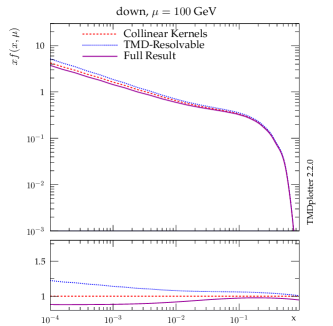
(a)

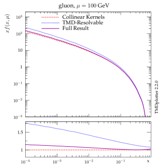
(b)

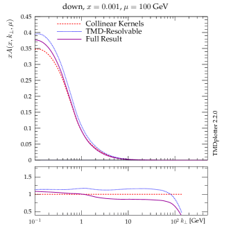
(c)

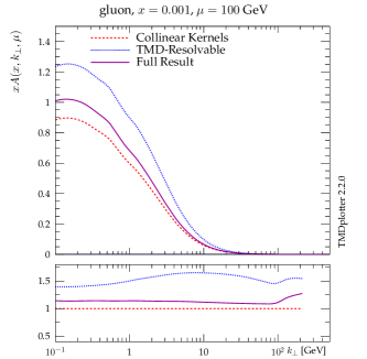
(d)

Figure 2: Evolution of the integrated (top) and TMD (bottom) parton distributions using the new branching equations with $k_{\perp}$-dependent splitting kernels. The solid magenta curves give the full result, while the dotted blue curves show the contribution to the full result from $k_{\perp}$-dependent splittings in resolvable emissions only. The dashed red curves show the result of evolution with purely collinear splitting kernels.

We next present numerical results from this MC solution of the branching evolution equations. For the purpose of illustrating the implementation of the branching evolution, we can take, as initial TMD distributions at scale $\mu_{0}$, any of the parameterizations available e.g. in the library [43, 44]. The numerical results which follow are obtained by taking the parameterization given in [45, 46] at $\mu_{0}=1.4$ GeV. In Fig. 2, the solid magenta curves show the results for gluon and down-quark TMD distributions evolved to $\mu=100$ GeV. In the top panels of Fig. 2 we plot the $x$ dependence of the distributions integrated over $k_{\perp}^{2}$, $f_{a}(x,\mu^{2})$, while in the bottom panels we plot the $k_{\perp}$ dependence for fixed $x$.

Fig. 2 presents, besides the solid magenta curves, two other sets of curves which are obtained with the same initial TMD distributions at scale $\mu_{0}$ but different evolution kernels, and are displayed for the purpose of comparison: the dashed red curves show the results which are obtained without including any $k_{\perp}$ dependence in the splitting kernels, that is, with the purely collinear splitting kernels; the dotted blue curves show the results which are obtained by including the $k_{\perp}$ dependence of splitting functions in resolvable emissions only.

The comparison of the full result (solid magenta) with the purely collinear result (dashed red) in Fig. 2 illustrates that the influence of the TMD splitting kernels on evolution is significant especially for low $x$. More particularly, it illustrates that the impact of the TMD splittings is not washed out by $k_{\perp}$-integration, and persists at the level of the distributions integrated over $k_{\perp}$ as well. We stress that the TMD distributions corresponding to the solid magenta curves and dashed red curves both fulfill the integral relations in Eq. (5). The differences between them stem from dynamical contributions encoded in the TMD splitting functions. These give rise to a change in the $k_{\perp}$ and $x$ shapes of the TMD distributions after evolution.

The comparison of the full result (solid magenta) with the result from including TMD splitting functions in resolvable emissions only (dotted blue) in Fig. 2 illustrates the decomposition of TMD splitting effects into resolvable and non-resolvable components. As implied by the analysis leading to Eq. (12), the TMD distributions corresponding to the dotted blue curves in Fig. 2 do not fulfill the integral relations in Eq. (5). Unlike the case described in the previous paragraph, therefore, the departure of the dotted blue curves from the full result can be attributed to violations of the relation (5).

	Full Result
$\mu^{2}$ (GeV2)	$\alpha_{s}(\mu^{2})$, fix. $z_{M}$	$\alpha_{s}(q_{\bot}^{2})$, fix. $z_{M}$	$\alpha_{s}(q_{\bot}^{2})$, dyn. $z_{M}$
3	1.000	1.000	1.000
10	0.999	0.999	0.999
$10^{2}$	0.997	0.996	0.997
$10^{3}$	0.994	0.992	0.994
$10^{4}$	0.991	0.987	0.991
$10^{5}$	0.984	0.978	0.983
	TMD-Resolvable
$\mu^{2}$ (GeV2)	$\alpha_{s}(\mu^{2})$, fix. $z_{M}$	$\alpha_{s}(q_{\bot}^{2})$, fix. $z_{M}$	$\alpha_{s}(q_{\bot}^{2})$, dyn. $z_{M}$
3	1.029	1.038	1.000
10	1.087	1.139	1.007
$10^{2}$	1.156	1.304	1.045
$10^{3}$	1.195	1.413	1.091
$10^{4}$	1.219	1.478	1.129
$10^{5}$	1.229	1.507	1.148
	Collinear Kernels
$\mu^{2}$ (GeV2)	$\alpha_{s}(\mu^{2})$ fix. $z_{M}$	$\alpha_{s}(q_{\bot}^{2})$, fix. $z_{M}$	$\alpha_{s}(q_{\bot}^{2})$, dyn. $z_{M}$
3	1.000	1.000	1.000
10	0.999	0.999	0.999
$10^{2}$	0.997	0.997	0.997
$10^{3}$	0.995	0.993	0.995
$10^{4}$	0.992	0.989	0.992
$10^{5}$	0.986	0.981	0.984

Table 1: Momentum sum rule check for (top) full result; (middle) result from $k_{\perp}$-dependent splittings in resolvable emissions only; (bottom) result from purely collinear splitting kernels. The three columns correspond to three different boundary conditions on the strong coupling $\alpha_{s}$ and soft-gluon resolution scale $z_{M}$.

To examine the size of these violations, in Tab. 1 we perform a numerical check of momentum sum rules. We present numerical results for $\sum_{a}\int_{x_{0}}^{1}dx\ xf_{a}(x,\mu^{2})$, where $x_{0}$ is a small fixed value. We have verified numerically the convergence of the result for decreasing $x_{0}$ and for the results in the Table we use $x_{0}=10^{-5}$. We report results for the three cases considered in Fig. 2, at different values of $\mu$. The three columns for each case correspond to different scenarios for the scale of the running coupling $\alpha_{s}$ and the soft-gluon resolution scale $z_{M}$: the first two have constant $z_{M}$ (“fix. $z_{M}$”) [46], one with $\alpha_{s}$ taken at the branching scale $\mu$ and one with $\alpha_{s}$ taken at the transverse momentum $q_{\perp}$, while the third has $\mu$-dependent (dynamical) $z_{M}$ (“dyn. $z_{M}$”) [37]. Consistently with the discussion above, the table shows that, regardless of the scenario for $\alpha_{s}$ and $z_{M}$, the momentum sum rule is satisfied, within the numerical accuracy, in the case of the branching evolution with TMD splitting functions proposed in this paper (top rows) as well as in the case of purely collinear splitting functions (bottom rows), while it is violated in the case of TMD splitting functions in real-emission kernels and collinear Sudakov factors (middle rows).

The numerical implementation of an approach which both includes the TMD splitting functions and satisfies the momentum sum rule is one of the main achievements of this paper. The construction of a full MC event generator implementing this approach, e.g. using the methods of [47], will be the subject of future work. Such a MC could be compared with existing small-$x$ MC generators based on high-energy factorization [48], e.g. [49, 50, 51, 52].

In conclusion, we have formulated a parton branching which is applicable to TMD and integrated distributions and for the first time takes into account both the $z$ and $k_{\perp}$ dependence of splitting functions defined from the high-energy limit of partonic decay processes. These (off-shell) splitting functions have well-prescribed collinear and high-energy limits: they coincide with the customary leading-order collinear splitting functions for $k_{\perp}\to 0$, and contain finite-$k_{\perp}$ corrections which are responsible for the all-order resummation of logarithmically enhanced contributions to parton evolution for $x\to 0$. We have introduced new Sudakov form factors, for both gluon and quark channels, depending on the angular-averaged TMD splitting functions. Using these elements, our approach describes resolvable and non-resolvable branchings. We have presented its MC implementation, and applied it to obtain numerical results for the evolution of TMD distributions, and to verify explicitly integral relations expressing the momentum sum rules.

Acknowledgments. We thank H. Jung for useful discussions. M. H. gratefully acknowledges support by Consejo Nacional de Ciencia y Tecnología grant number A1 S-43940 (CONACYT-SEP Ciencias Básicas). A. K. is grateful for the support of Narodowe Centrum Nauki under grant SONATAbis no 2019/34/E/ST2/00186. K. K. acknowledges the European Union’s Horizon 2020 research and innovation programme under grant agreement No. 824093. A. L. acknowledges funding by Research Foundation-Flanders (FWO) (application number: 1272421N). This work is supported partially by grant V03319N from the common FWO-PAS exchange program.

References

- [1] A. Buckley et al., arXiv:1902.01674 [hep-ph].
- [2] P. Azzi et al., CERN Yellow Rep. Monogr. 7 (2019) 1 [arXiv:1902.04070 [hep-ph]].
- [3] J. L. Feng et al., arXiv:2203.05090 [hep-ex].
- [4] P. Agostini et al. [LHeC and FCC-he Study Group], J. Phys. G 48 (2021) 110501 [arXiv:2007.14491 [hep-ex]].
- [5] Y. Hatta et al., arXiv:2002.12333 [hep-ph].
- [6] M. L. Mangano et al., CERN Yellow Rep. (2017) no.3, 1 [arXiv:1607.01831 [hep-ph]].
- [7] K. Kovařík, P.M. Nadolsky and D.E. Soper, Rev. Mod. Phys. 92 (2020) 045003 [arXiv:1905.06957 [hep-ph]].
- [8] R. Angeles-Martinez et al., Acta Phys. Polon. B 46 (2015) 2501 [arXiv:1507.05267 [hep-ph]].
- [9] X. Chen et al., arXiv:2203.01565 [hep-ph].
- [10] W. Bizon et al., JHEP 12 (2018) 132 [arXiv:1805.05916 [hep-ph]].
- [11] F. Hautmann et al., Phys. Lett. B 772 (2017) 446 [arXiv:1704.01757 [hep-ph]].
- [12] F. Hautmann et al., JHEP 1801 (2018) 070 [arXiv:1708.03279 [hep-ph]].
- [13] M. van Beekveld et al., arXiv:2205.02237 [hep-ph].
- [14] L. Gellersen, S. Höche and S. Prestel, arXiv:2110.05964 [hep-ph].
- [15] A. Bermudez Martinez, F. Hautmann and M. L. Mangano, Phys. Lett. B 822 (2021) 136700 [arXiv:2107.01224 [hep-ph]].
- [16] A. Bermudez Martinez, F. Hautmann and M. L. Mangano, arXiv:2109.08173 [hep-ph].
- [17] S. Gieseke, P. Stephens and B. Webber, JHEP 12 (2003) 045 [arXiv:hep-ph/0310083 [hep-ph]].
- [18] J. C. Collins, Acta Phys. Polon. B 34 (2003) 3103 [arXiv:hep-ph/0304122 [hep-ph]].
- [19] F. Hautmann, Phys. Lett. B 655 (2007) 26 [arXiv:hep-ph/0702196 [hep-ph]].
- [20] S. Catani and F. Hautmann, Nucl. Phys. B 427 (1994) 475 [arXiv:hep-ph/9405388 [hep-ph]].
- [21] S. Camarda et al., Eur. Phys. J. C 80 (2020) 251 [erratum: Eur. Phys. J. C 80 (2020) 440] [arXiv:1910.07049 [hep-ph]].
- [22] S. Camarda, L. Cieri and G. Ferrera, Phys. Rev. D 104 (2021) L111503 [arXiv:2103.04974 [hep-ph]].
- [23] F. Coradeschi and T. Cridge, Comput. Phys. Commun. 238 (2019) 262 [arXiv:1711.02083 [hep-ph]].
- [24] E. Accomando et al., Phys. Lett. B 803 (2020) 135293 [arXiv:1910.13759 [hep-ph]].
- [25] S. Catani and F. Hautmann, Phys. Lett. B 315 (1993) 157.
- [26] S. Taheri Monfared, F. Hautmann, H. Jung and M. Schmitz, PoS DIS2019 (2019) 136 [arXiv:1908.01621 [hep-ph]].
- [27] L. Keersmaekers, arXiv:2109.07326 [hep-ph].
- [28] V.N. Gribov and L.N. Lipatov, Sov. J. Nucl. Phys. 15 (1972) 438.
- [29] G. Altarelli and G. Parisi, Nucl. Phys. B126 (1977) 298.
- [30] Yu.L. Dokshitzer, Sov. J. Nucl. Phys. 46 (1977) 641.
- [31] E. A. Kuraev, L. N. Lipatov and V. S. Fadin, Sov. Phys. JETP 45 (1977) 199.
- [32] I. I. Balitsky and L. N. Lipatov, Sov. J. Nucl. Phys. 28 (1978) 822.
- [33] F. Hautmann, M. Hentschinski and H. Jung, Nucl. Phys. B 865 (2012) 54 [arXiv:1205.1759 [hep-ph]].
- [34] O. Gituliar, M. Hentschinski and K. Kutak, JHEP 01 (2016) 181 [arXiv:1511.08439 [hep-ph]].
- [35] M. Hentschinski, A. Kusina and K. Kutak, Phys. Rev. D 94 (2016) 114013 [arXiv:1607.01507 [hep-ph]].
- [36] M. Hentschinski, A. Kusina, K. Kutak and M. Serino, Eur. Phys. J. C 78 (2018) 174 [arXiv:1711.04587 [hep-ph]].
- [37] F. Hautmann, L. Keersmaekers, A. Lelek and A. M. Van Kampen, Nucl. Phys. B 949 (2019) 114795 [arXiv:1908.08524 [hep-ph]].
- [38] A. H. Mueller, B. W. Xiao and F. Yuan, Phys. Rev. D 88 (2013) 114010 [arXiv:1308.2993 [hep-ph]].
- [39] S. Marzani, Phys. Rev. D 93 (2016) 054047 [arXiv:1511.06039 [hep-ph]].
- [40] M. Nefedov, Phys. Rev. D 104 (2021) 054039 [arXiv:2105.13915 [hep-ph]].
- [41] M. Hentschinski, Phys. Rev. D 104 (2021) 054014 [arXiv:2107.06203 [hep-ph]].
- [42] T. Sjostrand, S. Mrenna and P.Z. Skands, JHEP 05 (2006) 026 [hep-ph/0603175].
- [43] N. A. Abdulov et al., Eur. Phys. J. C 81 (2021) 752 [arXiv:2103.09741 [hep-ph]].
- [44] F. Hautmann et al., Eur. Phys. J. C 74 (2014) 3220 [arXiv:1408.3015 [hep-ph]].
- [45] ZEUS, H1 Coll., Eur. Phys. J. C 75 (2015) 580 [arXiv:1506.06042 [hep-ex]].
- [46] A. Bermudez Martinez et al., Phys. Rev. D 99 (2019) 074008 [arXiv:1804.11152 [hep-ph]].
- [47] S. Baranov et al., Eur. Phys. J. C81 (2021) 425 [arXiv:2101.10221 [hep-ph]].
- [48] S. Catani, M. Ciafaloni and F. Hautmann, Nucl. Phys. B 366 (1991) 135.
- [49] H. Jung et al., Eur. Phys. J. C 70 (2010) 1237 [arXiv:1008.0152 [hep-ph]].
- [50] J. R. Andersen and J. M. Smillie, JHEP 06 (2011) 010 [arXiv:1101.5394 [hep-ph]].
- [51] G. Chachamis and A. Sabio Vera, Phys. Rev. D 93 (2016) 074004 [arXiv:1511.03548 [hep-ph]].
- [52] A. van Hameren, Comput. Phys. Commun. 224 (2018) 371 [arXiv:1611.00680 [hep-ph]].