Matrix-free Monolithic Multigrid Methods
for Stokes and Generalized Stokes Problems

Abstract

We consider the widely used continuous $\mathcal{Q}_{k}$-$\mathcal{Q}_{k-1}$ quadrilateral or hexahedral Taylor-Hood elements for the finite element discretization of the Stokes and generalized Stokes systems in two and three spatial dimensions. For the fast solution of the corresponding symmetric, but indefinite system of finite element equations, we propose and analyze matrix-free monolithic geometric multigrid solvers that are based on appropriately scaled Chebyshev-Jacobi smoothers. The analysis is based on results by Schöberl and Zulehner (2003). We present and discuss several numerical results for typical benchmark problems.

1 Introduction

The Stokes problem

$$-\mu\Delta u+\nabla p=f,\;\operatorname{div}u=0\;\mbox{in}\,\Omega,\;\mbox{and}\,u=u_{D}:=0\;\mbox{on}\,\partial\Omega$$ (1)

and the generalized Stokes problem

$$-\mu\Delta u+\gamma\varrho u+\nabla p=f,\;\operatorname{div}u=0\;\mbox{in}\,\Omega,\;\mbox{and}\,u=u_{D}:=0\;\mbox{on}\,\partial\Omega$$ (2)

are two important basic problems in fluid mechanics, where one looks for the velocity field $u=(u_{1},\dots,u_{d})$ and pressure field $p$ for some given right-hand side $f=(f_{1},\dots,f_{d})$, dynamic viscosity $\mu$, and density $\varrho$. For simplicity, we consider homogeneous Dirichlet date $u_{D}$ for the velocity in the analysis part of the paper, whereas non-homogeneous Dirichlet date $u_{D}$ are also permitted in our numerical studies presented in Section 4. Here, $d\in\{2,3\}$ denotes the space dimension. The non-negative parameter $\gamma$ depends on the time integration scheme, e.g., implicit Euler gives $\gamma=1/\Delta t$, and $\gamma=0$ formally turns the generalized Stokes problem (2) into the classical Stokes problem (1). The computational domain $\Omega\subset\mathbb{R}^{d}$ is supposed to be bounded and Lipschitz with boundary $\partial\Omega$. We mention that the Stokes problem arise from the iterative linearization of the stationary Navier-Stokes equations when treating the advection term on the right-hand side. The same idea leads to the generalized Stokes problem after an implicit time discretization of the instationary Navier-Stokes equations; see, e.g., [46]. Moreover, both problems are building blocks in fluid-structure interaction (FSI) problems where the Navier-Stokes equations model the fluid part; see, e.g., [38], [49], [23]. The Stokes problem itself can be used as model for describing dominantly viscous fluids. Thus fast solvers for the discrete surrogates of (1) or (2) are of great importance in many applications where the Navier-Stokes equations are involved. The mixed finite element discretization of (1) or (2) finally leads to large-scale linear systems of the form

$$\begin{pmatrix}A&B^{T}\\ B&-C\end{pmatrix}\begin{pmatrix}\mathbf{u}\\ \mathbf{p}\end{pmatrix}=\begin{pmatrix}\mathbf{f}\\ \mathbf{g}\end{pmatrix},$$ (3)

where here $\mathbf{u}\in\mathbb{R}^{n}$, $\mathbf{p}\in\mathbb{R}^{m}$, $\mathbf{f}\in\mathbb{R}^{n}$, and $\mathbf{g}\in\mathbb{R}^{m}$ are vectors, $A$ is a symmetric and positive definite (spd) $n\times n$ matrix, $C$ is a non-negative $m\times m$ matrix, $B^{T}$ is transposed to the $m\times n$ matrix $B$. Usually the matrix $C$ is $0$, but stabilizations can create a non-trivial matrix $C$; see, e.g., [16, 26].

The system matrix of (3) is symmetric, but indefinite. So special direct or iterative solvers tailored to these properties of the system matrix are needed; see, e.g., [39]. Iterative methods are most suited for large-scale systems as they usually arise after mixed finite element discretization. Similar to the Conjugate Gradient (CG) method in the case of spd systems, the MinRes [36] and the Bramble-Pasciak CG [7] are certainly efficient Krylov-subspace solvers for symmetric, indefinite systems of the form (3) provided that suitable preconditioners are available. We refer the reader to the survey article [4], the monograph [16], the more recent articles [33, 2, 34], and the references therein.
Monolithic geometric multigrid methods are another class of efficient solvers for large scale systems of finite element equations. The multigrid convergence analysis is based on the smoothing property and the approximation property; see [20]. In the case of symmetric, indefinite systems of the form (3), the construction of suitable smoothers is crucial for the overall efficiency of the multigrid method. Such smoothers range from low cost methods like Richardson-type iterations applied to the normal equation associated with (3), see [48, 9], collective smoothers, like Vanka-type smoothers, based on the solutions of small local problems, see [47, 41], to more expensive methods, whose costs for the Stokes problem are comparable with the costs of an optimal preconditioner for a discrete Laplace-like equation either in $\mathbf{p}$, like the exact and inexact Braess-Sarazin smoothers [6, 53] or, more recently in $\mathbf{u}$, resulting in better smoothing properties [10, 11]. A general framework for the construction and the analysis of smoothers was introduced in [50, 51] with the concept of transforming smoothers, which include several classes like distributive Gauss-Seidel smoothers. Yet another class of smoothers are Uzawa-type smoothers, see the survey article [14] (as well as the references therein), where also other classes of block smoothers are discussed.

In this paper, we are looking for an efficient (parallel) matrix-free implementation of all ingredients of Geometric MultiGrid (GMG) algorithms, which are based on a solid convergence analysis. Current developments of matrix-free solvers include problems in finite‐strain hyperelasticity [13], phase-field fracture [24, 25, 23], fluid-structure interaction [49], discontinuous Galerkin [28], compressible Navier-Stokes equations [19], incompressible Navier-Stokes and Stokes equations [17] as well as sustainable open-source code developments [32, 12], matrix-free implementations on locally refined meshes [31], and implementations on graphics processors [29].

Matrix-free implementations should avoid the assembling of all matrices involved in the multigrid algorithm. Matrix-free implementations can directly make use of the finite-difference-star representation of a matrix-vector multiplication especially, for finite difference or volume discretizations, or similarly the stencil representation of finite elemenet equations [3], or can be realized by the element matrices on the fly in the case of finite element discretizations; see, e.g., [27]. We are going to use the latter (element-based) matrix-free technique that leads not only to a considerable reduction of the memory demand, but also to a reduction of the arithmetical complexity, especially, for higher-order finite element discretizations; see, e.g., [32]. Moreover, element-based matrix-free techniques are very suited for the implementation on massively parallel computers with distributed memory [27]. On the other side, the element-based matrix-free technology restricts the use of smoothers mentioned above. Smoothers that are constructed from the assembled matrix are out of the game. We will consider inexact symmetric Uzawa smoothers (also known as a class of block approximate factorization smoothers) of the form

$$\hat{\mathbf{u}}^{j+1} =\mathbf{u}^{j}+{\hat{A}}^{-1}(\mathbf{f}-A\mathbf{u}^{j}-B^{T}\mathbf{p}^{j}),$$ (4)

$$\mathbf{p}^{j+1} =\mathbf{p}^{j}+{\hat{S}}^{-1}(B\hat{\mathbf{u}}^{j+1}-C\mathbf{p}^{j}-\mathbf{g}),$$ (5)

$$\mathbf{u}^{j+1} =\mathbf{u}^{j}+{\hat{A}}^{-1}(\mathbf{f}-A\hat{\mathbf{u}}^{j+1}-B^{T}\mathbf{p}^{j}),$$ (6)

which were analyzed by Schöberl and Zulehner in [41]. They showed the smoothing property provided that the spd “preconditioning” matrices $\hat{A}$ and $\hat{S}$ satisfy the spectral inequalities

$${\hat{A}}\geq A\quad\mbox{and}\quad{\hat{S}}\geq{\tilde{S}}=B{\hat{A}}^{-1}B^{T}+C,$$ (7)

and an additional estimate of the difference of the system matrix and the “preconditioning” matrix generated by the smoother (4) - (6). The W-cycle multigrid convergence then follows from this smoothing property and the approximation property. The application of ${\hat{A}}^{-1}$ and ${\hat{S}}^{-1}$ to vectors will be realized completely matrix-free by means of the Chebyshev-Jacobi method. Once the smoother can be performed matrix-free, the complete multigrid cycle can be implemented matrix-free and in parallel. The implementation is based on the deal.II finite element library [1], and in particular, the matrix-free and geometric multigrid modules [27, 22]. The parallel performance and scalability of matrix-free GMG solvers has widely been demonstrated; see, e.g., [28, 32, 13, 25, 31]. Hence, in this work, we mainly focus on the numerical analysis and the quantitative numerical illustration of the theoretical results.

The remainder of the paper is organized as follows. Section 2 provides the mixed variational formulation of (1) and (2), their mixed fined element discretization by means of inf-sup stable $\mathcal{Q}_{k}$-$\mathcal{Q}_{k-1}$ quadrilateral or hexahedral finite elements, and recalls some well-known results on solvability and discretization error estimates. In Section 3, we present the matrix-free GMG algorithm, in particular, the class of matrix-free smoothers we are going to use, and the analysis of the smoothing and approximation properties yielding W-cycle multigrid convergence. Section 4 presents and discusses our numerical results for different benchmark problems supporting the theoretical results. Finally, we draw some conclusions and give an outlook in Section 5.

2 Mixed Variational Formulation and Discretization

The mixed variational formulation of (1) or (2) read as follows: Find $u\in V=H^{1}_{0}(\Omega)^{d}$ and $p\in Q=L_{0}^{2}(\Omega)=\{q\in L^{2}(\Omega):\int_{\Omega}qdx=0\}$ such that

$$a(u,v)+b(v,p) =\langle F,v\rangle \forall v\in V,$$ (8)

$$b(u,q) =0 \forall q\in Q,$$ (9)

with

$$a(u,v) =\int_{\Omega}(\mu\,\nabla u:\nabla v+\gamma\varrho uv)\,dx,$$ (10)

$$b(u,q) =\int_{\Omega}q\,\operatorname{div}u\,dx,$$ (11)

$$\langle F,v\rangle =\int_{\Omega}fv\,dx.$$ (12)

In some applications, e.g., FSI, instead of the bilinear form (10), the bilinear form

$$a(u,v)=\int_{\Omega}(\mu\,\varepsilon(u):\varepsilon(v)+\gamma\varrho uv)\,dx,$$ (13)

is used, where $\varepsilon(u)=\frac{1}{2}(\nabla u+(\nabla u)^{T})$ denotes the deformation rate tensor, and $\mu$ and $\varrho$ may depend on the spatial variable $x$, but should always be uniformly positive and bounded; see, e.g., [49]. In both cases, the bilinear form $a(\cdot,\cdot)$ is elliptic and bounded on $V$. Since $F$ obviously belongs to the dual space $V^{*}$ of $V$, and since the bilinear form $b(\cdot,\cdot)$ is also bounded and fulfills the famous LBB (inf-sup) condition

$$\inf_{q\in Q\setminus\{0\}}\sup_{v\in V\setminus\{0\}}\frac{b(v,q)}{\|v\|_{H^{1}(\Omega)^{d}}\|q\|_{L^{2}(\Omega)}}\geq c>0,$$ (14)

the mixed variational problem (8) - (9) is well-posed, i.e. there exists a unique solution $(u,p)\in V\times Q$ satisfying an a priori estimate; see, e.g., [18, 44]. Throughout this paper, $c$ denotes a generic constant independent of the mesh level.

For later use we mention that the mixed variational problem (8) - (9) can also be written as a variational problem on $V\times Q$: Find $(u,p)\in V\times Q$ such that

$$\mathcal{B}((u,p),(v,q))=\langle F,v\rangle\quad\text{for all}\ (v,q)\in V\times Q$$ (15)

with the bilinear form

$$\mathcal{B}((w,r),(v,q))=a(w,v)+b(v,r)+b(w,q).$$

Figure 1: Construction of the tensor product nodes using a bilinear mapping $T_{\tau}$.

Let us now briefly describe the mixed finite element discretization of (8) - (9) by means of Taylor-Hood $\mathcal{Q}_{k}$-$\mathcal{Q}_{k-1}$ finite elements, i.e., continuous, piecewise polynomials of degree $k$ and $k-1$ in each coordinate direction, with $k\in\mathbb{N},k\geq 2$. We assume that the computational domain $\Omega$ can be decomposed into non-overlapping convex quadrilateral (hexahedral) elements $\tau\in\mathcal{T}_{h}$. Each of the elements $\tau\in\mathcal{T}_{h}$ is the image of the reference element $(0,1)^{d}$ by a bilinear (trilinear) transformation $T_{\tau}$. The nodal basis points for the shape functions are constructed using a tensor-product scheme on the reference element $(0,1)^{d}$ as visualized in Figure 1. This leads to the elementwise space

$$\mathcal{Q}_{k}(\tau):=\{\hat{u}\circ T_{\tau},\hat{u}\in\mathcal{Q}_{k}\},$$

and the corresponding global, continuous space

$$V_{h}:=\{v\in V:{\left.\kern-1.2pt{v}\vphantom{\big{|}}\right|_{\tau}}\in\mathcal{Q}_{k}(\tau)\quad\forall\tau\in\mathcal{T}_{h}\}.$$

The same construction is applied for the pressure space to obtain

$$\mathcal{Q}_{h}:=\{q\in Q\cap C(\Omega):{\left.\kern-1.2pt{q}\vphantom{\big{|}}\right|_{\tau}}\in\mathcal{Q}_{k-1}(\tau)\quad\forall\tau\in\mathcal{T}_{h}\}.$$

Since not all features of the geometry can be represented by this construction (e.g., circles), we adapt the mesh during refinement to resolve those entities; see Figure 2.

Figure 2: The mesh is gradually adapted to the geometry (left) during refinement.

Now the mixed finite element discretization of (8) - (9) reads as follows: Find $u_{h}\in V_{h}\subset V$ and $p_{h}\in Q_{h}\subset Q$ such that

$$a(u_{h},v_{h})+b(v_{h},p_{h}) =\langle F,v_{h}\rangle\quad\forall v_{h}\in V_{h},$$ (16)

$$b(u_{h},q_{h}) =0\quad\forall v_{h}\in Q_{h}.$$ (17)

Once the usual nodal basis is chosen in $V_{h}$ and $Q_{h}$, the finite element scheme (16) - (17) is equivalent to the linear system (3) with $C=0$ and $g=0$ that can be written in the compact form

$$\mathbf{K}\mathbf{x}=\mathbf{b},\quad\mbox{with}\;\mathbf{K}=\begin{pmatrix}A&B^{T}\\ B&0\end{pmatrix},\;\mathbf{x}=\begin{pmatrix}\mathbf{u}\\ \mathbf{p}\end{pmatrix},\mbox{ and }\mathbf{b}=\begin{pmatrix}\mathbf{f}\\ 0\end{pmatrix}.$$ (18)

The discrete inf-sup condition

$$\inf_{q_{h}\in Q_{h}\setminus\{0\}}\sup_{v_{h}\in V_{h}\setminus\{0\}}\frac{b(v_{h},q_{h})}{\|v_{h}\|_{H^{1}(\Omega)^{d}}\|q_{h}\|_{L^{2}(\Omega)}}\geq c>0,$$ (19)

ensures existence and uniqueness of the finite element solution $(u_{h},p_{h})\in V_{h}\times Q_{h}$, and the estimate of the discretization error by the best approximation error. The inf-sup condition is ensured for $d=2$ and all $k\geq 2$, see [43]. The inf-sup condition also holds for $d=3$ and all $k\geq 2$ under mild conditions on the mesh, if we restrict ourselves to affine linear transformations $T_{\tau}$. We refer the reader to Appendix A for the precise formulation of the conditions imposed on the mesh. As a consequence the following Cea-type discretization error estimate holds.

$$\|u-u_{h}\|_{H^{1}(\Omega)^{d}}+\|p-p_{h}\|_{L^{2}(\Omega)}\leq c\,\left(\inf_{v_{h}\in V_{h}}\|u-v_{h}\|_{H^{1}(\Omega)^{d}}+\inf_{q_{h}\in Q_{h}}\|p-g_{h}\|_{L^{2}(\Omega)}\right).$$

If $\Omega$ is convex or if its boundary is sufficiently smooth, it follows from the theory of elliptic regularity that $(u,p)$ even belongs to $H^{2}(\Omega)^{d}\times H^{1}(\Omega)$ and we have

$$\|u\|_{H^{2}(\Omega)^{d}}+\|p\|_{H^{1}(\Omega)}\leq c\,\|f\|_{L^{2}(\Omega)}.$$ (20)

Based on this elliptic regularity and a standard duality argument we additionally have the following error estimate in $L^{2}(\Omega)^{d}$:

$$\|u-u_{h}\|_{L^{2}(\Omega)^{d}}\leq c\,h\,\left(\|u-u_{h}\|_{H^{1}(\Omega)^{d}}+\|p-p_{h}\|_{L^{2}(\Omega)}\right),$$

where $h$ denotes the mesh size of $\mathcal{T}_{h}$; see, e.g., [26].

3 Matrix-free Geometric Multigrid Solvers

3.1 Multigrid Algorithm and its Matrix-Free Implementation

Now let us assume that there is a sequence of meshes $\mathcal{T}_{\ell}$, $\ell=0,1,...,L$, where the subindex $0$ denotes the coarsest mesh, and the subindex $L$ the finest mesh obtained after $L$ uniform mesh refinement steps. This sequence of meshes leads to a sequence of nested finite element spaces $V_{\ell}\times Q_{\ell}$.

The multigrid method starts on the finest level $L$, and recursively adapts the current solution by solving the equation on the coarser levels. The corrections are then prolongated back to the finer levels. A crucial component is the smoother, which is applied before and after switching levels. Sometimes the post-smoothing is omitted. Its main purpose is to ”smooth” the error, such that it can be represented on the coarser grids without losing too much accuracy. The scheme is illustrated in Algorithm 1. More details and the analysis for multigrid methods can be found in the standard literature; see, e.g., [20, 8].

1

2MG ($\mathbf{x}_{\ell},\mathbf{b}_{\ell}$)

3

4if $\ell=0$ then

      $\mathbf{x}_{\ell}\leftarrow\mathbf{K}^{-1}_{\ell}\mathbf{b}_{\ell}$;

       /* coarse grid solution */

5     

6      end if

7     

     $\mathbf{x}_{\ell}\leftarrow\mathcal{S}_{\ell}(\mathbf{x}_{\ell},\mathbf{b}_{\ell})$ ;

       /* pre-smoothing */

8     

     $\mathbf{r}_{\ell}\leftarrow\mathbf{b}_{\ell}-\mathbf{K}_{\ell}\mathbf{x}_{\ell}$ ;

       /* residual */

9     

     $\mathbf{r}_{\ell-1}\leftarrow\mathbf{I}^{\ell-1}_{\ell}\mathbf{r}_{\ell}$ ;

       /* restriction */

10     

11     $\mathbf{w}_{\ell-1}\leftarrow 0$

12     for $j=1,\dots,\gamma$ do

           $\mathbf{w}_{\ell-1}\leftarrow\textnormal{{MG}}(\mathbf{w}_{\ell-1},\mathbf{r}_{\ell-1})$;

            /* recursion */

13          

14           end for

15          

          $\mathbf{w}_{\ell}\leftarrow\mathbf{I}_{\ell-1}^{\ell}\mathbf{w}_{\ell-1}$;

            /* prolongation */

16          

          $\mathbf{x}_{\ell}\leftarrow\mathbf{x}_{\ell}+\mathbf{w}_{\ell}$;

            /* correction */

17          

          $\mathbf{x}_{\ell}\leftarrow\mathcal{S}_{\ell}(\mathbf{x}_{\ell},\mathbf{b}_{\ell})$;

            /* post-smoothing */

18          

19          return $\mathbf{x}_{\ell}$

Algorithm 1 Multigrid method for the solution of $\mathbf{K}_{\ell}\mathbf{x}_{\ell}=\mathbf{b}_{\ell}$.

GMG methods are particularly suited for matrix-free applications since the entries of the matrix $\mathbf{K}=\mathbf{K}_{\ell}$ (we omit the level subindex where it is not needed) are actually not required. Therefore, we would like to avoid the assembly of the huge sparse matrix $\mathbf{K}$ and its subsequent multiplications with a vector $\mathbf{x}$. Rather, we assemble the result $\mathbf{Kx}$ directly, i.e.,

$${\mathbf{Kx}=\sum_{\tau\in\mathcal{T}}\mathbf{P}_{\tau}\mathbf{K}_{\tau}\mathbf{P}_{\tau}^{T}\mathbf{x},}$$

with the local-to-global mapping $\mathbf{P}_{\tau}$, and the element matrices $\mathbf{K}_{\tau}$. While this already captures the main idea of matrix-free methods, further optimizations are required to reach a competitive performance. These details are explained in great detail in the work [27, 28, 32, 12], and are readily included in the deal.II library [1]. The further optimizations include the mapping of the element-wise contributions $\mathbf{K}_{\tau}$ to the reference domain. Therein, the tensor product structure of the shape functions is exploited via sum-factorization. Thus, even the assembly of the dense local element matrices $\mathbf{K}_{\tau}$ can be replaced by efficient sum-factorization techniques; see, e.g., [30, 27]. This leads to a very promising computational complexity for matrix-vector multiplication, in particular for high polynomial degree shape functions. There, we only need $\mathcal{O}(d^{2}(p+1)(1-\frac{1}{p+1})^{-d})$ operations per dof compared to $\mathcal{O}((p+1)^{d})$ for a sparse matrix based approach; see [27]. Furthermore, the workload is split across multiple compute nodes using MPI, and accelerated by explicit vectorization, i.e., multiple elements are handled simultaneously with a single CPU instruction. The operators on each level of the GMG method can be represented by such a matrix-free procedure.

The convergence rate of the multigrid method given by Algorithm 1 is determined by the smoothing property and the approximation property; see [20]. In order to prove the convergence of the $W$-cycle, it is enough to investigate the convergence of the $(\ell-(\ell-1))$ two-grid method which is defined by Algorithm 1 when $\mathbf{w}_{\ell-1}\leftarrow\textnormal{{MG}}(\mathbf{w}_{\ell-1},\mathbf{r}_{\ell-1})$ is replaced by the exact solution $\mathbf{w}_{\ell-1}\leftarrow\mathbf{K}^{-1}_{\ell-1}\mathbf{r}_{\ell-1}$ of the coarse grid system $\mathbf{K}_{\ell-1}\mathbf{x}_{\ell-1}=\mathbf{r}_{\ell-1}$ in step 10. In the algebraic setting, the two-grid iteration operator has the form

$$\mathbf{M}_{\ell}^{\ell-1}=\mathbf{S}_{\ell}^{m}(\mathbf{I}_{\ell}-\mathbf{I}_{\ell-1}^{\ell}\mathbf{K}_{\ell-1}^{-1}\mathbf{I}_{\ell}^{\ell-1}\mathbf{K}_{\ell})\mathbf{S}_{\ell}^{m}=\mathbf{S}_{\ell}^{m}\mathbf{C}_{\ell}^{\ell-1}\mathbf{S}_{\ell}^{m}$$ (21)

where $\mathbf{I}_{\ell}$ is the identity matrix, $\mathbf{C}_{\ell}^{\ell-1}=\mathbf{I}_{\ell}-\mathbf{I}_{\ell-1}^{\ell}\mathbf{K}_{\ell-1}^{-1}\mathbf{I}_{\ell}^{\ell-1}\mathbf{K}_{\ell}$ is the coarse-grid-correction operator, $\mathbf{S}_{\ell}$ denotes the iteration operator of the smoother, $m$ is the number of pre- and post-smoothing steps of some symmetric smoother $\mathcal{S}_{\ell}$ as defined in (4) - (6). Here, $\mathbf{M}_{\ell}^{\ell-1}$, $\mathbf{C}_{\ell}^{\ell-1}$, and $\mathbf{S}_{\ell}$ are linear operators on $X_{\ell}=\mathbb{R}^{N_{\ell}}$ with $N_{\ell}=\dim V_{\ell}+\dim Q_{\ell}$. If there is no post-smoothing, i.e. $\mathbf{M}_{\ell}^{\ell-1}=\mathbf{C}_{\ell}^{\ell-1}\mathbf{S}_{\ell}^{m}$, then two-grid convergence rate estimate

$$\|\mathbf{M}_{\ell}^{\ell-1}\|_{L(X_{\ell},X_{\ell})}\leq\|\mathbf{C}_{\ell}^{\ell-1}\mathbf{K}_{\ell}^{-1}\|_{L(X_{\ell}^{*},X_{\ell})}\,\|\mathbf{K}_{\ell}\mathbf{S}_{\ell}^{m}\|_{L(X_{\ell},X_{\ell}^{*})}\leq c\,\eta(m)=:\sigma(m)$$ (22)

follows from the approximation property

$$\|\mathbf{C}_{\ell}^{\ell-1}\mathbf{K}_{\ell}^{-1}\|_{L(X_{\ell}^{*},X_{\ell})}\leq c,$$ (23)

and the smoothing property

$$\|\mathbf{K}_{\ell}\mathbf{S}_{\ell}^{m}\|_{L(X_{\ell},X_{\ell}^{*})}\leq\eta(m),$$ (24)

where $\|\cdot\|_{L(Y,Z)}$ denotes the standard operator norm, $\mathbf{K}_{\ell}$ is interpreted as a linear operator from $X_{\ell}$ to its dual $X_{\ell}^{*}$ and $X_{\ell}=\mathbb{R}^{N_{\ell}}$ is equipped with a suitable mesh-dependent vector norm $\|\cdot\|_{X_{\ell}}$ in which we want to study the multigrid convergence, $c$ is some positive constant, and the non-negative function $\eta(m)$ converges to $0$ for $m$ tending to infinity. Both $c$ and $\eta$ are independent of level index $\ell$. Due to these properties, $\sigma(m)$ becomes smaller than $1$ for sufficiently many smoothing steps, and the two grid-method converges at least with the rate $\sigma(m)$. The convergence of the $W$- and the generalized $V$-cycles then easily follows from a perturbation argument; see [20]. We note that the convergence of the pure $V$-cycle is not covered by this theory. In the next subsection, we prove the approximation property (23), whereas, in Subsection 3.3, we propose several matrix-free smoothers, and prove the smoothing property (24).

3.2 Approximation Property

For the prolongation operator $\mathbf{I}_{\ell-1}^{\ell}$ we use the matrix representation of the canocical injection from $V_{\ell-1}\times Q_{\ell-1}$ to $V_{\ell}\times Q_{\ell}$, and set $\mathbf{I}_{\ell}^{\ell-1}=\left(\mathbf{I}_{\ell-1}^{\ell}\right)^{T}$ for the restriction operator. As already pointed out, we need to specify a mesh-dependent norm $\|\cdot\|_{X_{\ell}}$ on $X_{\ell}=\mathbb{R}^{N_{\ell}}$. Let $h_{\ell}$ be the mesh size of $\mathcal{T}_{\ell}$. Then we set

$$\|\mathbf{y}_{\ell}\|_{X_{\ell}}=\left(h_{\ell}^{d-2}\|\mathbf{v}_{\ell}\|^{2}+h_{\ell}^{d}\|\mathbf{q}_{\ell}\|^{2}\right)^{1/2}\quad\text{for}\ \mathbf{y}_{\ell}=\begin{pmatrix}\mathbf{v}_{\ell}\\ \mathbf{q}_{\ell}\end{pmatrix}\in X_{\ell}=\mathbb{R}^{N_{\ell}},$$ (25)

where $\|\cdot\|$ denotes the Euclidean norm of vectors. If $\mathbf{v}_{\ell}$ and $\mathbf{q}_{\ell}$ are the vector representations of some elements $v_{\ell}\in V_{\ell}$ and $q_{\ell}\in Q_{\ell}$, respectively, then it is easy to see that $\|\mathbf{y}_{\ell}\|_{X_{\ell}}$ and $\|(v_{\ell},q_{\ell})\|_{0,\ell}$, given by

$$\|(v_{\ell},q_{\ell})\|_{0,\ell}=\left(h_{\ell}^{-2}\|v_{\ell}\|_{L^{2}(\Omega)^{d}}^{2}+\|q_{\ell}\|_{L^{2}(\Omega)}^{2}\|\right)^{1/2},\quad\text{for}\,(v_{\ell},q_{\ell})\in V_{\ell}\times Q_{\ell},$$

are equivalent norms, in short

$$\|\mathbf{y}_{\ell}\|_{X_{\ell}}\sim\|(v_{\ell},q_{\ell})\|_{0,\ell}.$$

Associated with this norm on $V_{\ell}\times Q_{\ell}$ and the bilinear form $\mathcal{B}$, a second mesh-dependent norm on $V_{\ell}\times Q_{\ell}$ is introduced by

$$\|(v_{\ell},q_{\ell})\|_{2,\ell}=\sup_{0\neq(w_{\ell},r_{\ell})\in V_{\ell}\times Q_{\ell}}\frac{\mathcal{B}((v_{\ell},q_{\ell}),(w_{\ell},r_{\ell}))}{\|(w_{\ell},r_{\ell})\|_{0,\ell}}\quad\text{for}\,(v_{\ell},q_{\ell})\in V_{\ell}\times Q_{\ell}.$$

Obviously, $\|(v_{\ell},q_{\ell})\|_{2,\ell}$ and $\|\mathbf{K}_{\ell}\mathbf{y}_{\ell}\|_{X_{\ell}^{*}}$ are equivalent norms, too, i.e.,

$$\|(v_{\ell},q_{\ell})\|_{2,\ell}\sim\|\mathbf{K}_{\ell}\mathbf{y}_{\ell}\|_{X_{\ell}^{*}},$$

where $\|\cdot\|_{X_{\ell}^{*}}$ denotes the norm in $X_{\ell}^{*}$ dual to $\|\cdot\|_{X_{\ell}}$.

Observe that $\mathbf{K}_{\ell-1}^{-1}\mathbf{I}_{\ell}^{\ell-1}\mathbf{K}_{\ell}$ is the matrix representation of the Ritz projection $R_{\ell}^{\ell-1}$ from $V_{\ell}\times Q_{\ell}$ onto $V_{\ell-1}\times Q_{\ell-1}$, given by

$$\mathcal{B}(R_{\ell}^{\ell-1}(v_{\ell},q_{\ell}),(w_{\ell-1},r_{\ell-1}))=\mathcal{B}((v_{\ell},q_{\ell}),(w_{\ell-1},r_{\ell-1})),$$

for all $(v_{\ell},q_{\ell})\in V_{\ell}\times Q_{\ell}$ and $(w_{\ell-1},r_{\ell-1})\in V_{\ell-1}\times Q_{\ell-1}$. Under the assumption of elliptic regularity the approximation property was shown in [48] in the following form.

$$\|[I-R_{\ell}^{\ell-1}](v_{\ell},q_{\ell})\|_{0,\ell}\leq c\,\|(v_{\ell},q_{\ell})\|_{2,\ell}\quad\text{for all}\ (v_{\ell},q_{\ell})\in V_{\ell}\times Q_{\ell},$$

with a constant $c$ which is independent of the level $\ell$. Therefore,

$$\|\mathbf{C}_{\ell}^{\ell-1}\mathbf{y}_{\ell}\|_{X_{\ell}}\sim\|[I-R_{\ell}^{\ell-1}](v_{\ell},q_{\ell})\|_{0,\ell}\leq c\,\|(v_{\ell},q_{\ell})\|_{2,\ell}\sim c\,\|\mathbf{K}_{\ell}\mathbf{y}_{\ell}\|_{X_{\ell}^{*}}\quad\text{for all}\ \mathbf{y}_{\ell}\in X_{\ell},$$

which immediately implies the approximation property of the form (23).

3.3 Matrix-free Smoothers and Smoothing Property

We now introduce different classes of properly scaled Chebyshev-Jacobi smoothers, which allow an efficient matrix-free implementation, and investigate their smoothing property. Since the smoothers are living only on one level, we omit the level subindex $\ell$ throughout this subsection.

3.3.1 Scaled Chebyshev-Jacobi Smoothers

The main challenge of a matrix-free implementation of the GMG algorithm is connected with an appropriate smoother that must permit an efficient matrix-free implementation as well. Since the matrix entries are not at our disposal, many classical methods like (block)-Gauss-Seidel, (block)-Jacobi, or ILU, are not applicable. Rather, we should look for smoothing methods that only require matrix-vector operations. One class of methods that seems to be predestined for this task are polynomial methods. This approach yields smoothers that are based on a matrix polynomial $s_{k_{C}}(C)$ of the degree $k_{C}$ . Such a polynomial can be efficiently applied by only performing matrix-vector multiplications with the matrix-free operator $C$.

We can further improve the situation by precomputing the diagonal of a matrix-free operator, which enables us to use Jacobi-based methods. The diagonal can be computed efficiently using the deal.II matrix-free framework, and storing it comes at the cost of only one additional vector. In fact, we will use the Jacobi-method, and improve its smoothing property by means of polynomial acceleration.

For a matrix-free implementation, our choices for $\hat{A}$ and $\hat{S}$ in (4)–(6) are focused on Chebyshev-Jacobi smoothers for the realization of matrix-free application of $\hat{A}^{-1}$ and $\hat{S}^{-1}$ to vectors.

For a linear system of the form $Mx=b$ with some (simple) preconditioner $D$ these smoothers are semi-iterative algorithms of the form

$$\tilde{x}=x+s_{k}(D^{-1}M)D^{-1}(b-Mx)$$

with $s_{k}(t)=(1-T_{k+1}(t))t^{-1}$ and $T_{k+1}(t):={C_{k+1}(\frac{\beta+\alpha-2t}{\beta-\alpha})}/{C_{k+1}(\frac{\beta+\alpha}{\beta-\alpha})},$ where $C_{k+1}$ denotes the Chebyshev polynomial of the first kind of degree $k+1$. We note that, in this subsection, the subindex $k$ is related to the degree of the Chebyshev polynomial and not to the polynomial degree of the shape functions used for constructing the finite element spaces $\mathcal{Q}_{k}$-$\mathcal{Q}_{k-1}$ introduced in Section2. Later we will again add the subindex that indicates the matrix to which the polynom belongs as we did above with $k_{C}$. The interval $[\alpha,\beta]$ contains the high energy eigenvalues of $D^{-1}M$. In particular, we will use $[\alpha,\beta]=[\beta/2,\beta]$ with $\beta=\lambda_{\text{max}}(D^{-1}M)$. Actually, in the numerical tests, a close approximation of $\lambda_{\text{max}}(D^{-1}M)$ will be used for $\beta$. The iteration matrix for the Chebyshev-Jacobi method is then given by $T_{k+1}(D^{-1}M)$ with associated preconditioner $C_{M}^{-1}=\operatorname{Cheb}(M,D,k)=s_{k}(D^{-1}M)D^{-1}$. The Chebyshev-Jacobi method is easy to apply by exploiting a three-term recurrence relation, see, e.g., [39]. For $k=0$, it corresponds to the damped Jacobi method with damping parameter $\omega=2/(\alpha+\beta)$ and the iteration matrix $T_{1}(D^{-1}M)=I-\omega D^{-1}M$.

The next lemma contains two important estimates for the Chebyshev-Jacobi smoother, which are required for the scaling of the smoother and the proof of the smoothing property.

Lemma 1.

Let $M$ and $D$ be symmetric and positive definite matrices, $k\in\mathbb{N}_{0}$, and $\alpha,\beta\in\mathbb{R}$ with $0<\alpha<\beta=\lambda_{\text{max}}(D^{-1}M)$. Then the following estimates hold.

$$c_{1}\,M\leq C_{M}\quad\text{and}\quad C_{M}\leq c_{2}\,\beta\,D,$$

where

$$c_{1}=\left(1+\frac{1}{C_{k+1}(\bar{s})}\right)^{-1},\quad c_{2}=\left(1-\frac{1}{C_{k+1}(\bar{s})}\right)^{-1}$$

with $\bar{s}=(\beta+\alpha)/(\beta-\alpha)$.

Proof.

We have

$$M^{1/2}C_{M}^{-1}M^{1/2} =M^{1/2}s_{k}(D^{-1}M)D^{-1}M^{1/2}=s_{k}(M^{1/2}D^{-1}M^{1/2})M^{1/2}D^{-1}M^{1/2}$$

$$\leq\lambda_{\text{max}}\left(s_{k}(M^{1/2}D^{-1}M^{1/2})M^{1/2}D^{-1}M^{1/2}\right)\,I$$

Since $\sigma(M^{1/2}D^{-1}M^{1/2})=\sigma(D^{-1}M)\subset[0,\beta]$, we immediately obtain

$$\lambda_{\text{max}}\left(s_{k}(M^{1/2}D^{-1}M^{1/2})M^{1/2}D^{-1}M^{1/2}\right)\leq\max_{\lambda\in[0,\beta]}\left(s_{k}(\lambda)\,\lambda\right)=1+\frac{1}{C_{k+1}(\bar{s})}=\frac{1}{c_{1}},$$

which proves the first inequality.

For the second inequality, we proceed in a similar way. We obtain

$$D^{1/2}C_{M}^{-1}D^{1/2} =D^{1/2}s_{k}(D^{-1}M)D^{-1}D^{1/2}=s_{k}(D^{-1/2}MD^{-1/2})$$

$$\geq\lambda_{\text{min}}\left(s_{k}(D^{-1/2}MD^{-1/2})\right)\,I$$

and

$$\lambda_{\text{min}}\left(s_{k}(D^{-1/2}MD^{-1/2})\right)\geq\min_{\lambda\in[0,\beta]}s_{k}(\lambda)\geq\frac{1}{\beta}\left(1-\frac{1}{C_{k+1}(\bar{s})}\right)=\frac{1}{c_{2}\beta},$$

which completes the proof of the second inequality. The used bounds involving the polynomial $s_{k}$ follow easily from well-known properties of Chebyshev polynomials. ∎

Note that, for a fixed ratio $\alpha/\beta$, the quantities $c_{1}$ and $c_{2}$ in Lemma 1 depend only on $k$ and approach 1 for $k$ approaching $\infty$.

With these notations we set

$$\hat{A}^{-1}=\sigma\,\operatorname{Cheb}(A,D_{A},k_{A})$$

with $D_{A}:=\operatorname{diag}(A)$, $\beta=\lambda_{\text{max}}(D_{A}^{-1}A)$, $\alpha=\beta/2$, and $\sigma=c_{1}=c_{1}(k_{A},\alpha,\beta)$ according to Lemma 1, which guarantees $\hat{A}\geq A$.

In principle the same construction could be carried out for $\hat{S}$ leading to

$$\hat{S}^{-1}=\tau\,\operatorname{Cheb}(\tilde{S},D_{\tilde{S}},k_{S})$$

with $\tilde{S}=B\hat{A}^{-1}B^{T}$, $D_{\tilde{S}}:=\operatorname{diag}(\tilde{S})$, $\beta=\lambda_{\text{max}}(D_{\tilde{S}}^{-1}\tilde{S})$, $\alpha=\beta/2$, and $\tau=c_{1}=c_{1}(k_{S},\alpha,\beta)$ according to Lemma 1, which guarantees $\hat{S}\geq\tilde{S}$. However, obtaining $\operatorname{diag}(\tilde{S})$ as required for the Chebyshev-Jacobi smoother is more expensive, since it involves the inverse $\hat{A}^{-1}$. Hence, we aim to replace $D_{\tilde{S}}$ by cheaper approximations, namely

$$\tilde{D}_{\tilde{S}_{d}} :=\operatorname{diag}(\tilde{S}_{d})\quad\text{with}\quad\tilde{S}_{d}:=B(\operatorname{diag}(A))^{-1}B^{T},$$ (26)

$$\tilde{D}_{\tilde{S}_{p}} :=\operatorname{diag}(\tilde{S}_{p})\quad\text{with}\quad\tilde{S}_{p}:=M_{p},$$ (27)

$$\tilde{D}_{\tilde{S}_{loc}} :=\sum_{\tau\in\mathcal{T}_{h}}P_{\tau}^{T}{\operatorname{diag}(B_{\tau}(\operatorname{diag}(A_{\tau}))^{-1}B_{\tau}^{T})P_{\tau},}$$ (28)

where $M_{p}$ denotes the pressure mass matrix, and where the local-to-global matrices $P_{\tau}$ were defined before. The approximation $\tilde{D}_{\tilde{S}_{loc}}$ computes the diagonal $\operatorname{diag}(B_{\tau}(\operatorname{diag}(A_{\tau}))^{-1}B_{\tau}^{T})$ locally on each element $\tau$ and assembles it together. The computation of $\tilde{D}_{\tilde{S}_{d}}$ still requires to assemble the sparse matrix $B$, in order to compute $(\tilde{D}_{\tilde{S}_{d}})_{ii}=\sum_{j}B_{ij}^{2}(\operatorname{diag}(A)_{jj})^{-1}$. Thus, in order to keep the smoother fully matrix-free, the choices $\tilde{D}_{\tilde{S}_{p}}$ and $\tilde{D}_{\tilde{S}_{loc}}$ are preferred.

The setup of the ingredients of the smoother is summarized in Algorithm 2. The smoother (4) - (6) with $\hat{A}$ and $\hat{S}$ defined by Algorithm 2 can be written in the compact form

$$\mathbf{x}^{j+1}=\mathbf{x}^{j}+\mathbf{\hat{K}}^{-1}[\mathbf{b}-\mathbf{K}\mathbf{x}^{j}]$$ (29)

with

$$\mathbf{\hat{K}}=\begin{pmatrix}\hat{A}&B^{T}\\ B&B\hat{A}^{-1}B^{T}-\hat{S}\end{pmatrix}$$

The iteration matrix $\mathbf{S}$ of the smoother (29) is obviously given by $\mathbf{S}=\mathbf{I}-\mathbf{\hat{K}}^{-1}\mathbf{K}$. We note that, in Algorithm 2, $\bar{s}=3$ for the standard choice $\alpha=\beta/2$.

1

Input : $k_{A},k_{S}$

2

3

/* Velocity part */

4

5$D_{A}\leftarrow\operatorname{diag}(A)$

6$\beta\leftarrow\lambda_{max}(D_{A}^{-1}A)$

7$\alpha\leftarrow\beta/2$

8$C_{A}^{-1}\leftarrow\operatorname{Cheb}(A,D_{A},k_{A})$

9$\sigma=\frac{C_{k_{A}+1}(\bar{s})}{1+C_{k_{A}+1}(\bar{s})}$

$\hat{A}^{-1}\leftarrow\sigma\,C_{A}^{-1}$;

  /* scale Chebyshev to guarantee $\hat{A}\geq A$ */

10

/* Pressure part */

11

$\tilde{D}_{\tilde{S}}\leftarrow\tilde{D}_{\tilde{S}_{d}},\tilde{D}_{\tilde{S}_{p}},$ or $\tilde{D}_{\tilde{S}_{loc}}$;

  /* see (26),(27), or (28) */

12

13$\beta\leftarrow\rho(\tilde{D}_{\tilde{S}}^{-1}\tilde{S})$

14$\alpha=\beta/2$

15$C_{S}^{-1}\leftarrow Cheb(\tilde{S},\tilde{D}_{\tilde{S}},k_{S})$

16$\tau=\frac{C_{k_{S}+1}(\bar{s})}{1+C_{k_{S}+1}(\bar{s})}$

$\hat{S}^{-1}\leftarrow\tau\,C_{S}^{-1}$;

  /* scale Chebyshev to guarantee $\hat{S}\geq\tilde{S}$ */

17

18

19return $\hat{A}^{-1},\hat{S}^{-1}$

Algorithm 2 Setup of the smoother for the Stokes problem.

3.3.2 Smoothing Property

Since we can always ensure by scaling that the ingredients $\hat{A}$ and $\hat{S}$ of $\mathbf{\hat{K}}$ satisfy the spectral inequalities (7) for all choices proposed in Subsection 3.3.1, Theorem 7 from [14] (see also Theorem 3 in [41]) delivers the estimate

$$\|\mathbf{K}\mathbf{S}^{m}\|_{L(X_{\ell},X_{\ell}^{*})}\leq\eta_{0}(m-1)\,\|\mathbf{\hat{K}}-\mathbf{K}\|_{L(X_{\ell},X_{\ell}^{*})}$$ (30)

with

$$\eta_{0}(m)=\frac{1}{2^{m}}\binom{m}{\lfloor(m+1)/2\rfloor}\leq\left\{\begin{array}[]{ll}\sqrt{\displaystyle\frac{2}{\pi m}}&\text{for even }m,\\ \sqrt{\displaystyle\frac{2}{\pi(m+1)}}&\text{for odd }m,\end{array}\right.$$

where $\binom{m}{\ell}$ denotes the binomial coefficient, and $\lfloor x\rfloor$ is nothing but the largest integer less or equal to $x\in\mathbb{R}$.

It remains to show that

$$\|\mathbf{\hat{K}}-\mathbf{K}\|_{L(X_{\ell},X_{\ell}^{*})}\leq c$$ (31)

to get the smoothing property (24) with $\eta(m)=c\eta_{0}(m)=O(1/\sqrt{m})$, where $c$ is some non-negative constant that should be independent of the level index $\ell$. Indeed, following [41], we can proceed as follows: First we note that

$$\mathbf{\hat{K}}-\mathbf{K}=\begin{pmatrix}\hat{A}-A&0\\ 0&\hat{S}-\tilde{S}\end{pmatrix}.$$

Therefore, it follows from the definition (25) of the norm in $X_{\ell}$ that

$$\|\mathbf{\hat{K}}-\mathbf{K}\|_{L(X_{\ell},X_{\ell}^{*})} =\max\left(h^{-(d-2)}\|\hat{A}-A\|,h^{-d}\|\hat{S}-\tilde{S}\|\right)$$

$$\leq\max\left(h^{-(d-2)}\|\hat{A}\|,h^{-d}\|\hat{S}\|\right),$$

where here the matrix norm $\|\cdot\|$ is the spectral norm that is associated to the Euclidean vector norm. So, (31) holds, if

$$h^{-(d-2)}\|\hat{A}\|\leq c\quad\text{and}\quad h^{-d}\|\hat{S}\|.$$

We start with the verification of the first estimate

$$h^{-(d-2)}\|\hat{A}\|\leq c.$$ (32)

From Lemma 1 with $M=\hat{A}$ and $D=D_{A}$, it follows that

$$\hat{A}\leq\frac{c_{2}}{c_{1}}\,\lambda_{\text{max}}(D_{A}^{-1}A)\,D_{A},$$

which leads to $\|\hat{A}\|\leq(c_{2}/c_{1})\,\lambda_{\text{max}}(D_{A}^{-1}A)\|D_{A}\|$. In order to conclude from this estimate that (32) holds for some constant $c$ independent of the mesh level, it suffices to show that

$$A\leq c\,D_{A}\quad\text{and}\quad\|D_{A}\|\leq c\,h^{d-2}.$$

The first part, which is equivalent to $\lambda_{\text{max}}(D_{A}^{-1}A)\leq c$, follows, e.g., from [21, Theorem 12.20] by exploiting the sparsity pattern on $A$, whereas the second part can easily be obtained by a standard scaling argument.

Next we discuss the second estimate

$$h^{-d}\|\hat{S}\|\leq c$$

with $\hat{S}^{-1}=\tau\,\operatorname{Cheb}(\tilde{S},\tilde{D}_{S},k_{S})$ and the three different choices for $\tilde{D}_{S}$ given by (26), (27), and (28). For each case it follows from Lemma 1 that $\|\hat{S}\|\leq(c_{2}/c_{1})\,\lambda_{\text{max}}(\tilde{D}_{S}^{-1}\tilde{S})\|\tilde{D}_{S}\|$. As before it suffices to show that

$$\tilde{S}\leq c\,\tilde{D}_{S}\quad\text{and}\quad\|\tilde{D}_{S}\|\leq c\,h^{d}.$$ (33)

We will discuss these conditions for each of the three choices for $\tilde{D}_{S}$ separately.

1. We start with the choice $\tilde{D}_{S}=\tilde{D}_{\tilde{S}_{p}}=\operatorname{diag}(M_{p})$. The coercivity of the bilinear form $a(\cdot,\cdot)$ and the boundedness of the bilinear form $b(\cdot,\cdot)$ yield the estimate

   $$\sup_{v_{h}\in V_{h}}\frac{b(v_{h},q_{h})^{2}}{a(v_{h},v_{h})}\leq c\,\|q_{h}\|_{L^{2}(\Omega)}^{2},$$

   or, equivalently, in matrix notation,

   $$BA^{-1}B^{T}\leq c\,M_{p}.$$

   From the scaling condition $\hat{A}\geq A$, we obtain the following upper bound of $\tilde{S}$.

   $$\tilde{S}=B\hat{A}^{-1}B^{T}\leq BA^{-1}B^{T}\leq c\,M_{p}.$$

   As before by exploting the sparsity pattern of $M_{p}$ and by using a standard scaling argument it follows that

   $$M_{p}\leq c\,\operatorname{diag}(M_{p})\quad\text{and}\quad\|\operatorname{diag}(M_{p})\|\leq ch^{d},$$

   which, together with $\tilde{S}\leq c\,M_{p}$, directly yield the required estimates (33).

2. Next we discuss the choice $\tilde{D}_{S}=\tilde{D}_{\tilde{S}_{d}}=\operatorname{diag}(B(\operatorname{diag}(A))^{-1}B^{T})$. It suffices to show that

   $$\tilde{D}_{\tilde{S}_{d}}\sim\tilde{D}_{\tilde{S}_{p}}.$$

   Then the estimates (33) follow directly from the previous case $\tilde{D}_{S}=\tilde{D}_{\tilde{S}_{p}}$.

   For $v_{h}\in V_{h}$ and $q_{h}\in Q_{h}$, we have

   $$b(v_{h},q_{h})=-\int_{\Omega}q_{h}\operatorname{div}v_{h}\ dx=\int_{\Omega}v_{h}\cdot\nabla q_{h}\ dx$$

   via integration by parts, which in turn implies

   $$\sup_{v_{h}\in V_{h}}\frac{b(v_{h},q_{h})}{\|v_{h}\|_{L^{2}(\Omega)^{d}}}\leq\|\nabla q_{h}\|_{L^{2}(\Omega)},$$

   or, equivalently, in matrix notation

   $$BM_{v}^{-1}B^{T}\leq K_{p},$$

   where $M_{v}$ is the mass matrix in $V_{h}$ and $K_{p}$ is the matrix representing the $H^{1}$-seminorm in $Q_{h}$. A reverse inequality of the form

   $$BM_{v}^{-1}B^{T}\gtrsim\,K_{p}$$

   also holds, see (35). Therefore we have

   $$BM_{v}^{-1}B^{T}\sim K_{p}.$$

   Here we used the following notation for symmetric matrices $M$, $N$: $M\lesssim N$ if there is a constant $c>0$ such that $M\leq c\,N$, $M\gtrsim N$ if $N\lesssim M$, and $M\sim N$ if $M\lesssim N$ and $M\gtrsim N$. The involved constants are meant to be independent of the mesh level.

   A standard scaling argument gives

   $$\operatorname{diag}(A)\sim h^{-2}\,M_{v}.$$

   Hence

   $$B(\operatorname{diag}(A))^{-1}B^{T}\sim h^{2}BM_{v}^{-1}B^{T}\sim h^{2}\,K_{p}$$

   and

   $$\tilde{D}_{S}=\operatorname{diag}(B(\operatorname{diag}(A))^{-1}B^{T})\sim h^{2}\,\operatorname{diag}(K_{p})\sim\operatorname{diag}(M_{p})=\tilde{D}_{\tilde{S}_{p}},$$

   which concludes the discussion of this case.

3. For the choice $\tilde{D}_{S}=\tilde{D}_{\tilde{S}_{loc}}=\sum_{\tau\in\mathcal{T}}P_{\tau}^{T}\operatorname{diag}(B_{\tau}(\operatorname{diag}(A_{\tau}))^{-1}B_{\tau}^{T})P_{\tau}$ we procede similarly to the previous case: We have, see (35),

   $$B_{\tau}M_{v,\tau}^{-1}B_{\tau}^{\top}\gtrsim K_{p,\tau}.$$

   An inequality in reverse direction

   $$B_{\tau}M_{v,\tau}^{-1}B_{\tau}^{\top}\lesssim h_{\tau}^{-2}M_{p,\tau}$$

   follows from a standard scaling argument. These two estimates imply

   $$h_{\tau}^{-2}\operatorname{diag}(M_{p,\tau})\sim\operatorname{diag}(K_{p,\tau})\lesssim\operatorname{diag}\left(B_{\tau}M_{v,\tau}^{-1}B_{\tau}^{\top}\right)\lesssim h_{\tau}^{-2}\operatorname{diag}(M_{p,\tau}).$$

   Therefore,

   $$\operatorname{diag}\left(B_{\tau}M_{v,\tau}^{-1}B_{\tau}^{\top}\right)\sim h_{\tau}^{-2}\operatorname{diag}(M_{p,\tau})$$

   and

   $$\sum_{\tau\in\mathcal{T}_{h}}P_{\tau}^{T}\operatorname{diag}(B_{\tau}(\operatorname{diag}(A_{\tau}))^{-1}B_{\tau}^{T})P_{\tau}$$

   $$\quad\sim\sum_{\tau\in\mathcal{T}_{h}}h^{2}\,P_{\tau}^{T}\operatorname{diag}(B_{\tau}M_{v,\tau}^{-1}B_{\tau}^{T})P_{\tau}\sim\sum_{\tau\in\mathcal{T}_{h}}P_{\tau}^{T}\operatorname{diag}(M_{p,\tau})P_{\tau}\sim\operatorname{diag}(M_{p}).$$

   We have shown that

   $$\tilde{D}_{\tilde{S}_{loc}}=\sum_{\tau\in\mathcal{T}_{h}}P_{\tau}^{T}\operatorname{diag}(B_{\tau}(\operatorname{diag}(A_{\tau}))^{-1}B_{\tau}^{T})P_{\tau}\sim\operatorname{diag}(M_{p})=\tilde{D}_{\tilde{S}_{p}},$$

   which concludes the discussion of the last case.

4 Numerical Results

In this section, we perform some numerical experiments in two and three spatial dimensions in order to illustrate and quantify the theoretical results. First, the numerical setting is described. Then we present the results of extensive numerical tests for the unit square with homogeneous Dirichlet boundary conditions and some right-hand side force, typical benchmark problems, namely the driven cavity Stokes problem in 2d and 3d, the 2d Stokes flow around a cylinder, and finally the 2d instationary driven cavity Stokes problem with implicit time discretization of which leads to the solution of a generalized Stokes problem at every time step.

4.1 Numerical Setting and Programming Code

The code is implemented in C++ using the open-source finite element library deal.II [1], and in particular, their matrix-free and geometric multigrid components; see [12, 27]. For the GMG method, we use a W-cycle with an equal number of pre- and post-smoothing steps, which will be varied in the numerical experiments. On the coarsest grid, we assemble the sparse matrix and apply a direct method for solving the algebraic system. This is feasible due to the small amount of dofs on $\mathcal{T}_{\ell=0}$. For more complex geometries yielding more dofs on the coarse grid $\mathcal{T}_{0}$, iterative solvers might be a more suitable and more efficient alternative. In all computations presented below, the finite element discretization is always done by inf-sup stable $\mathcal{Q}_{2}$-$\mathcal{Q}_{1}$ elements on quadrilateral and hexahedral meshes in two and three spatial dimensions, respectively.

In order to measure the multigrid convergence rate $\sigma(m)$, we perform $i\leq 15$ iterations of the multigrid solver until a reduction of the initial residual by $10^{-10}$ is achieved. Since the first few steps usually yield a much better reduction compared to the later iterations, we only consider the average reduction $q$ of the last $3$ steps; see, e.g., [45]. Hence, we compute

$$q=\left(\frac{r^{j}}{r^{j-3}}\right)^{\frac{1}{3}},$$

where $r^{j}=\|\mathbf{b}-\mathbf{Kx}^{j}\|$ denotes the residual after $j$ GMG iterations, with the initial guess $\mathbf{x}^{0}=\mathbf{0}$.

For the timings, we report the time $T$ needed to reduce the error by $\varepsilon=10^{-1}$, i.e.,

$$T(\varepsilon)=T_{iter}\frac{\log(\varepsilon)}{\log(q)},$$

with the time for a single iteration $T_{iter}$ and the respective reduction rate $q$ obtained as described before. The experiments were done on one node of our local hpc cluster Radon1, equipped with a Intel(R) Xeon(R) Silver 4214R CPU with 2.40GHz and 128 GB of RAM.

4.2 Laser beam material processing

In order to substantiate our theoretical setting, we first consider an example with homogeneous Dirichlet boundary conditions. The background of this example is in laser material processing; see for instance [35]. Therein, various physics interact in which the heated material can be modeled with the help of viscous flow (here Stokes). Concentrating on the fluid component only, the laser beam is mathematically modeled by a non-homogeneous right-hand side point force that is here represented by a smoothed Gaussian curve.

4.2.1 Geometry, Boundary Conditions, Parameters, and Right Hand Side

The domain is the unit square $(0,1)^{2}$. For the boundary conditions we have $u_{D}=(0,0)^{T}$. The (dynamic) viscosity is given by $\mu=0.0022$. Given the point $x_{0}=(0.75,0.75)\in\Omega$, the right hand side $f$ of (1) is given by

$$f=\begin{pmatrix}f_{1}\\ f_{2}\end{pmatrix}=\begin{pmatrix}0\\ c_{1}\exp(-c_{2}(x-x_{0})^{2})\end{pmatrix},\quad x\in\Omega,$$ (34)

with $c_{1}=0.001$ and $c_{2}=100$. Figure 3 illustrates the computed solutions.

Figure 3: Laser beam material processing: Computed solution of the first test case. (a) x-velocity, (b) y-velocity, (c) pressure

4.2.2 Results for Different Diagonal Approximations

We start with comparing the convergence rates using the different approximations for $\tilde{D}_{\tilde{S}}$ which are visualized in Figure 4. For the $A$-block, we can easily compute $D_{A}=\operatorname{diag}(A)$ and, hence, apply $\hat{A}^{-1}:=\hat{\sigma}C_{A}^{-1}$. However, for the Schur-complement part, computing the exact diagonal $D_{\tilde{S}}$ is computationally expensive since it involves $\hat{A}^{-1}$. Hence, in (26), (27), and (28), we suggested several approximations $\tilde{D}_{S}$, which are visualized in Figure 4. We here consider only $2467$ dofs since we want to compare different cheaper approximations with the expensive diagonal $D_{\tilde{S}}$. The plot only shows the results for the Jacobi setting ($k=0$) and the Chebyshev-Jacobi degrees $k=3$, but the behavior is similar for other polynomial degrees in between, and will be investigated later on in the more complex examples. We can see that using any of the approximations $\tilde{D}_{S}$ yields mostly similar rates as the exact diagonal $D_{\tilde{S}}$. In any case, increasing the number of smoothing steps improves the convergence rate of the multigrid solver. In the Jacobi case presented in top-left corner of Figure 4, this is not obvious from the plot. However, for sufficiently many smoothing steps, the expected behavior $q\sim 1/\sqrt{m}$ is attained.

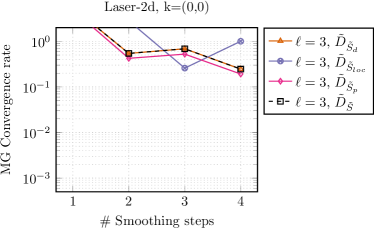
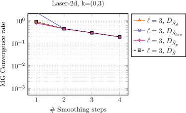
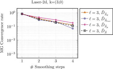
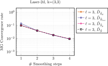
Figure 4: Laser beam material processing: Convergence rates for different diagonal approximations of the Schur complement and various Chebyshev polynomial degrees.

4.3 2d Driven Cavity

The second example deals with the stationary Lid-Driven Cavity flow [42, 52]; see also the benchmark collection of TU Dortmund.

4.3.1 Geometry, Boundary conditions, and Parameters

The computational domain is given by the unit square $\Omega=(0,1)^{2}$. The flow is driven by a prescribed velocity $u_{D}=(1,0)^{T}$ on the top boundary $\Gamma_{top}$, and $u_{D}=(0,0)^{T}$ on the remaining part $\partial\Omega\backslash\Gamma_{top}$ of the boundary $\partial\Omega$ of $\Omega$; see Figure 5 for a visualization of this setting. We first consider the stationary Stokes problem (1), with the the viscosity $\mu=1$ and the right-hand side $f=0$.

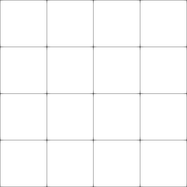
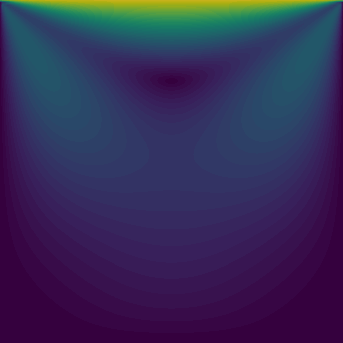
Figure 5: 2d Driven Cavity: Geometry, coarse grid, and velocity field of the computed solution.

4.3.2 Different diagonal approximations of the Schur Complement

Again, we investigate the effect of the approximations (26), (27), and (28) replacing the computationally expensive diagonal $D_{\tilde{S}}$. The convergence rates using the different approximations for $\tilde{D}_{\tilde{S}}$ are visualized in Figure 6. We here consider only $2467$ dofs since we want to compare different cheaper approximations with the expensive diagonal $D_{\tilde{S}}$. The plot only shows the results for the Jacobi setting ($k=0$) and the Chebyshev-Jacobi degrees $k=3$, but the behavior is similar for other polynomial degrees in between, and will be investigated afterwards. We can see that using $\tilde{D}_{\tilde{S}_{d}}$ yields very similar rates as the exact diagonal $D_{\tilde{S}}$ for most degrees. Furthermore, using the pressure approximations works very well in this example. This might be due to the simple tensor-product geometry. In the Schäfer-Turek benchmark later on, this choice still works but is less effective. The locally computed diagonals fall slightly behind, most likely due to the missing contributions from neighboring elements. In any case, increasing the number of smoothing steps improves the convergence rate of the multigrid solver. In the Jacobi case given in the top-left corner of Figure 6, this is not obvious from the plot. However, for sufficiently many smoothing steps, the expected behavior $q\sim 1/\sqrt{m}$ is attained.

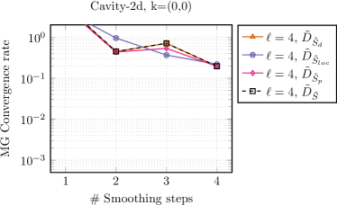
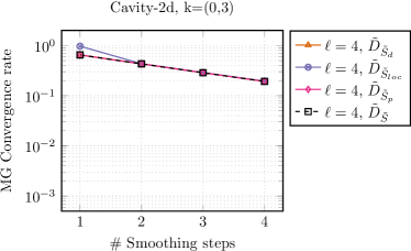
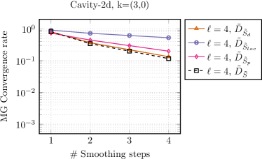
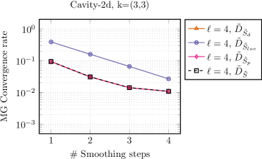
Figure 6: 2d Driven Cavity: Convergence rates for different diagonal approximations of the Schur complement and various Chebyshev polynomial degrees.

4.3.3 Different Polynomial Degrees

Next, we look at the influence of the polynomial degrees $k_{A}$ and $k_{S}$ of the Chebyshev smoother. Higher values improve the reduction but come at additional costs in the application. The convergence rates are visualized in Figure 7 for the diagonal approximation $\tilde{D}_{\tilde{S}_{d}}$.

In Figure 8, we additionally consider the time that is needed for the application of the smoother. We note that increasing the degree of the Chebyshev polynomial may not improve the convergence rates enough to justify the increased computational effort. We present the achievable reduction of the residual per second for a fixed problem size of $148\,739$ dofs. The convergence rates stay constant during $h$-refinement, but the cost of applying the smoother grows linearly with the number of dofs. A hyphen denotes configurations that did not yield a convergent algorithm, e.g., because an insufficient number of smoothing steps has been performed. We can see that the additional cost of higher Chebyshev degrees does not necessarily pay off. Rather, the best performance is achieved for degrees $(1,1),(2,1)$ with two smoothing steps and $(3,2)$ with one smoothing step.

4.3.4 $W$-cycle versus $V$-cycle

The use of the $V$-cycle instead of the $W$-cycle yields almost the same convergence rates, but the $V$-cycle is cheaper; see Figure 8 (b). To stay in line with the multigrid convergence analysis provided in Section 3, we mainly use the $W$-cycle here. However, for practical purposes, it is advisable to use a $V$-cycle for better performance.

Figure 7: 2d Driven Cavity: Convergence rates for varying Chebyshev degrees and smoothing steps.

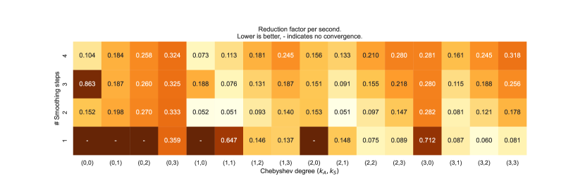
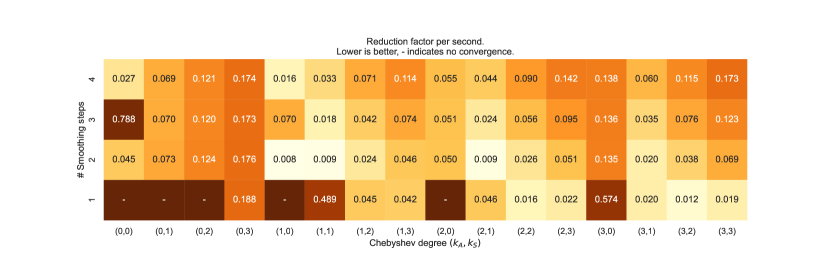
Figure 8: 2d Driven Cavity: Reduction factor per second: (a) W-cycle, (b) V-cycle.

4.4 Schäfer-Turek Benchmark 2d-1

In the third series of numerical tests, we apply the matrix-free geometrical multigrid solvers proposed and investigated in Section 3 to the well-known Schäfer-Turek benchmark; see [40].

4.4.1 Geometry, Boundary Conditions, and Parameters

The flow inside the channel $(0,2.2)\times(0,0.41)$ around the circular obstacle that is located at $(0.2,0.2)$ with diameter $0.1$ is driven by the given velocity $u_{D}=(v_{in}(x_{2}),0)$ on the left boundary $\Gamma_{in}$, with zero volume forces $f=0$. The inflow profile is prescribed as $v_{in}(x_{2})=4\,v_{\text{max}}\,x_{2}\,(0.41-x_{2})(0.41)^{-2}$ with the maximum velocity $v_{max}=1$. The velocity is zero on the top and bottom parts $\Gamma_{wall}$, as well as on the cylinder boundary $\Gamma_{c}$ (no-slip conditions). Figure 9 provides an illustration of the computational geometry, the mesh, and the computed velocity and the pressure fields. This example is again stationary ($\gamma=0$) with viscosity $\mu=1$.

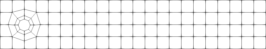
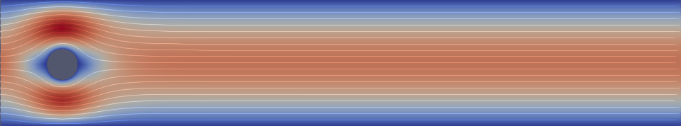
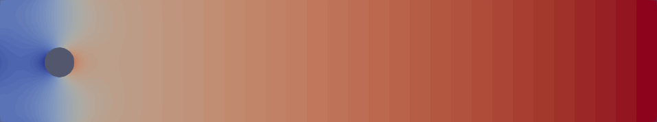
Figure 9: Schäfer-Turek: Geometry, coarse grid, velocity, and pressure field of the Schäfer-Turek benchmark.

4.4.2 Different Diagonal Approximations of the Schur Complement

As in the first example, we first consider a relatively coarse discretization with $3900$ fine grid dofs, and compare the various diagonal approximations (26), (27), and (28), in Figure 10. We can see that four smoothing steps are not enough to yield a convergent multigrid method in the Jacobi case $k_{A}=k_{S}=0$. Similar to the example before, the diagonal approximation $\tilde{D}_{\tilde{S}_{d}}$ yields almost the same rates as the exact variant $D_{\tilde{S}}$. The locally assembled diagonal $\tilde{D}_{\tilde{S}_{loc}}$ results in consistently worse convergence rates. In this example, the pressure approximation does not work as well as in the 2d driven cavity test case, with the surprising exception of $k=(3,3)$ and three smoothing steps. So far, we have no explanation for this behavior.

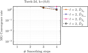
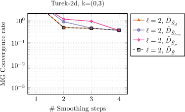
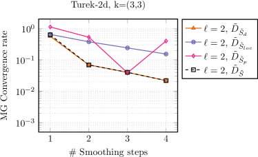
Figure 10: Schäfer-Turek: Convergence rates for different diagonal approximations and Chebyshev degrees.

4.4.3 Different Polynomial Degrees and more Unknowns

In the case of more refinement levels resulting in $232\,800$ fine grid dofs, the convergence rates for all tested combinations of $k_{A},k_{S},$ and $m$ are visualized in the heatmap shown in Figure 11. In contrary to the 2d driven cavity example, a single smoothing step is not enough to guarantee convergence even in the case $k_{A}=k_{S}=3$. From Figure 12, we deduce that two smoothing steps with degrees $k_{A}=3$ and $k_{S}=1$ yield the best reduction per second, and hence, the fastest overall solver.

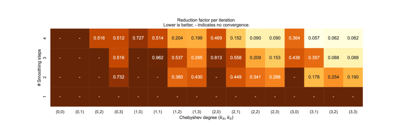
Figure 11: Schäfer-Turek: Convergence rates for varying Chebyshev degrees and smoothing steps.

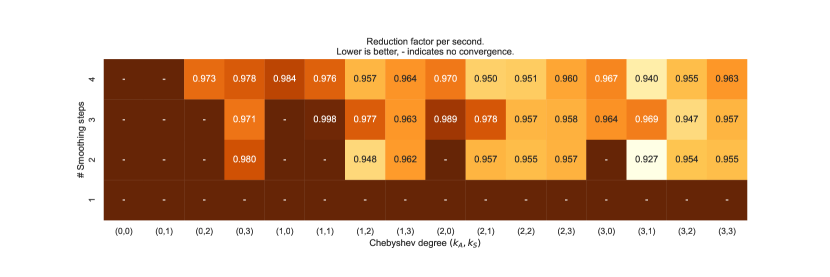
Figure 12: Schäfer-Turek: Reduction factor per second.

4.5 3d Driven Cavity

In the fourth series of numerical tests, we illustrate the performance of the smoother on a $3d$ extension of the lid-driven cavity benchmark from Subsection 4.3.

4.5.1 Geometry, Boundary conditions, and Parameters

The computational domain is nothing but the unit cube $\Omega=(0,1)^{3}$. The fluid is driven by the constant velocity $u_{D}=(1,0,0)$ on the top boundary $\Gamma_{top}=(0,1)\times(0,1)\times\{1\}$. On the remaining boundary we prescribe $u_{D}=0$. Figure 13 illustrates the geometry, the mesh, and the computed solution for the stationary Stokes problem (1), with $\mu=1$ and $f=0$.

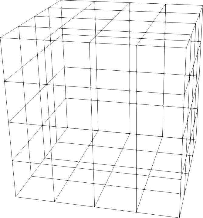
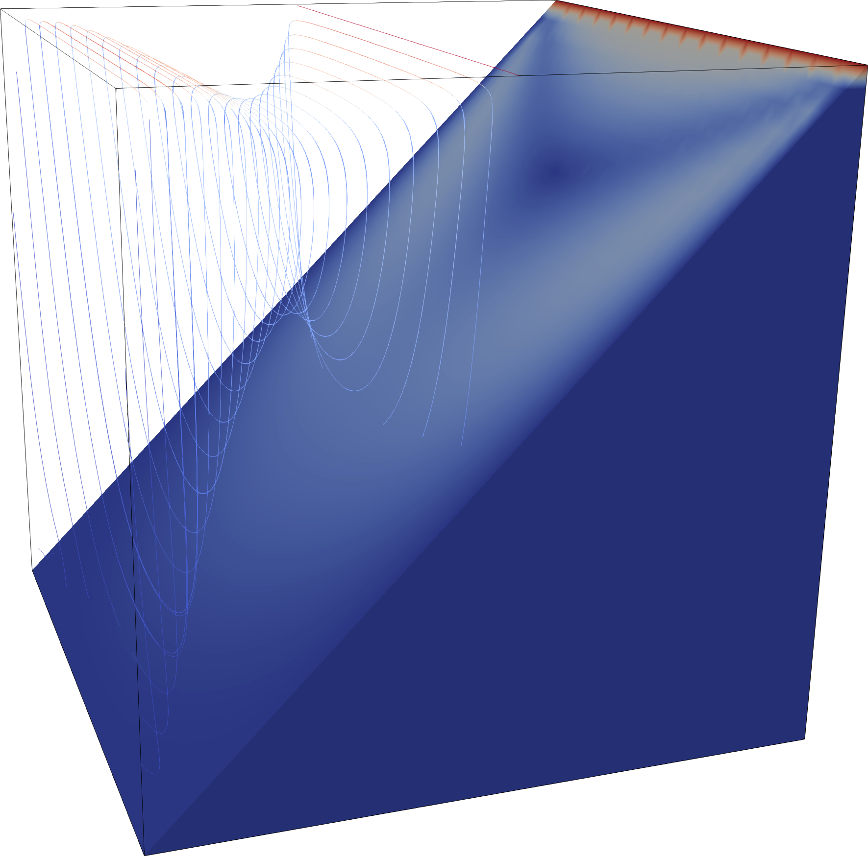
Figure 13: 3d Driven Cavity: Geometry, coarse grid, and velocity field of the solution for the Lid-Driven Cavity benchmark in $3d$.

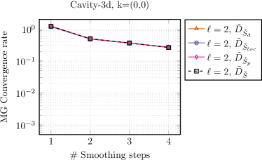
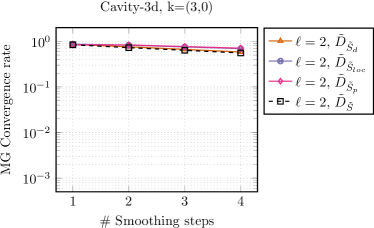
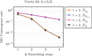
Figure 14: 3d Driven Cavity: Convergence rates for different diagonal approximations and various Chebyshev degrees.

4.5.2 Discussion of the Numerical Behavior of the Solver

For the computations, we used a problem size of $2312$ dofs for the comparison of the diagonals, and $112\,724$ dofs for the convergence rate and timing test. The results in $3d$ are in line with previous observations as shown in the Figures 15 and 16. Interestingly, $k=(3,0)$ yields worse rates compared to $k=(0,3)$ or the plain Jacobi setting, which was not the case in the 2d example. The highest reduction per second is again achieved with two smoothing steps of the $(1,1)$ Chebyshev smoother.

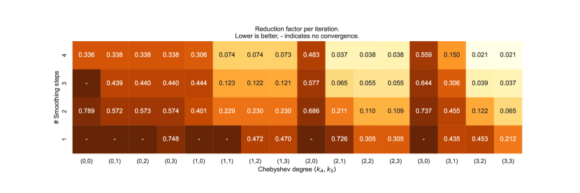
Figure 15: 3d Driven Cavity: Convergence rates for varying Chebyshev degrees and smoothing steps.

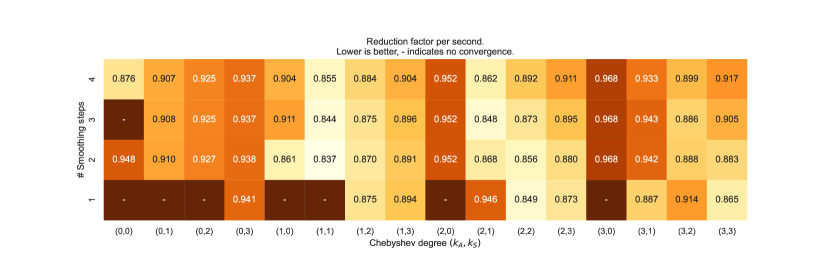
Figure 16: 3d Driven Cavity: Reduction factor per second.

4.6 Generalized Stokes Problem

The last series of numerical experiments is devoted to the numerical solution of the generalized Stokes problem (2) arising from the implicit Euler discretization of the instationary Stokes equations for the $2d$ driven cavity problem.

4.6.1 Configuration

The basic setting is the same as in Subsection 4.3. In addition, we now work with $\gamma=1/\Delta t$ arising from the time discretization. Moreover, we consider time-step sizes $\Delta t=1$ and $\Delta t=0.01$, with homogeneous initial conditions at $t=0$. We only present the results for a single time step here. However, the convergence rates stay the same for longer simulations as expected.

4.6.2 Discussion of the Numerical Behavior of the Solver

From Figure 17, we can see that the convergence rates for $\Delta t=1$ and $\Delta t=0.01$ are almost indistinguishable from each other, and also match with the results in Figure 7 ($\Delta t=\infty$). Thus, also the reduction per second is the same, since the additional mass matrix stemming from the time discretization does not impose a significant overhead.

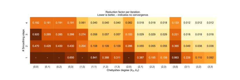
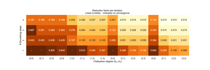
Figure 17: Time-dependent 2d Driven Cavity Problem: Convergence rates for varying Chebyshev degrees and smoothing steps. (a) $\Delta t=1$, (b) $\Delta t=0.01$.

5 Conclusions and Outlook

We proposed and analyzed matrix-free, monolithic geometric multigrid solvers that work for Stokes and generalized Stokes problems as the numerical studies performed for different well-known benchmark problems showed. In particular, the Chebyshev acceleration in $\hat{A}$ and $\hat{S}$ improves the smoothing property of the symmetric inexact Uzawa smoother (4) - (6) considerable. Indeed, increasing the polynomial degree of the Chebyshev smoother improves the convergence rates significantly, with moderate increase in the computational effort. The best performance requires a fine tuning between the number of smoothing steps and the degrees of the Chebyshev smoothers. However, choosing a high degree (e.g., $3$) yields very similar performance and is a good default initial choice. Although we did not present parallel studies in this paper, the code runs efficiently in parallel with excellent strong scalability. The parallelization is done without changes in the results beyond floating point errors. Hence, all convergence rates are independent of the number of utilized cores.

The Stokes and generalized Stokes solvers discussed in this paper can also be used for solving stationary and instationary Navier-Stokes problems, and as building block in solvers or preconditioners for other coupled problems involving flow, such as fluid-structure interaction or Boussinesq approximations for laser-beam material processing or convection of material in the earth’s mantle. However, then we have to treat the convection term on the right-hand side. So, we cannot expect robustness of the solver with respect to dominating convection. The Oseen or the Newton linearizations that takes care of the convection also lead to systems of the form (18), but with an non-symmetric and, in general, non-positive definite matrix $A$. This changes the game completely. The theory for [41] is not applicable anymore. It is certainly a challenge to develop a theory that allows us to analyze this case. One possible approach is to use Reusken’s lemma, which allows to study the smoothing property also in the non-symmetric case, see [37, 15].

Appendix

Appendix A Discrete inf-sup Conditions

Here we assume that $\mathcal{T}_{h}$ is a subdivison of $\Omega$ such that each $\tau\in\mathcal{T}_{h}$ satisfies the following conditions.

In 2d:

$\tau=T_{\tau}((0,1)^{2})$ is a convex quadrilateral, $T_{\tau}$ bilinear, and $\overline{\tau}$ has at most two edges on $\partial\Omega$, among them there is no pair of opposite edges.

In 3d:

$\tau=T_{\tau}((0,1)^{3})$ is a parallelepiped, $T_{\tau}$ affine linear, and $\overline{\tau}$ has at most three faces on $\partial\Omega$, among them there is no pair of opposite faces.

Furthermore, we assume that the standard compatibity and shape regularity conditions hold for $\mathcal{T}_{h}$.

Then we have for the Taylor-Hood $\mathcal{Q}_{k}$-$\mathcal{Q}_{k-1}$ finite element the following results.

Theorem 1.

Let $k\in\mathbb{N}$ with $k\geq 2$. Then there is a constant $c>0$ such that

$$\sup_{0\neq v_{h}\in V_{h}}\frac{\displaystyle b(v_{h},q_{h})}{\|v_{h}\|_{H^{1}(\Omega)^{d}}}\geq c\,\|q_{h}\|_{L^{2}(\Omega)}\quad\text{for all}\ q_{h}\in Q_{h}.$$

This is equivalent to the classical inf-sup condition (14).

The next inf-sup condition has its origin in [5] and is formulated for a different pair of norms.

Theorem 2.

Let $k\in\mathbb{N}$ with $k\geq 2$. Then there is a constant $c>0$ such that for all $\tau\in\mathcal{T}_{h}$

$$\sup_{0\neq v_{h}\in V_{h}}\frac{\displaystyle b(v_{h},q_{h})}{\|v_{h}\|_{L^{2}(\Omega)^{d}}}\geq c\,\|\nabla q_{h}\|_{L^{2}(\Omega)^{d}}\quad\text{for all}\ q_{h}\in Q_{h}.$$

The proofs in [5] were restricted to meshes of rectangles in 2d resp. bricks in 3d.

We need also the following local version of Theorem 2.

Theorem 3.

Let $k\in\mathbb{N}$ with $k\geq 2$. Then there is a constant $c>0$ such that

$$\sup_{0\neq v_{h}\in V_{\tau}}\frac{\displaystyle b_{\tau}(v_{h},q_{h})}{\|v_{h}\|_{L^{2}(\tau)^{d}}}\geq c\,\|\nabla q_{h}\|_{L^{2}(\tau)^{d}}\quad\text{for all}\ q_{h}\in Q_{\tau}$$

with

$$b_{\tau}(v,q)=-\int_{\tau}q\,\operatorname{div}v\ dx,\quad V_{\tau}=\{v|_{\tau}\colon v\in V_{h}\},\quad Q_{\tau}=\{q|_{\tau}\colon q\in Q_{h}\}.$$

The last two theorems translate to the following estimates in matrix notation.

$$BM_{v}^{-1}B^{\top}\geq c^{2}\,K_{p}\quad\text{and}\quad B_{\tau}M_{v,\tau}^{-1}B_{\tau}^{\top}\geq c^{2}\,K_{p,\tau}.$$ (35)

For proofs of Theorems 1, 2, and 3, see [54] For a proof of Theorem 1 in 2d see also [43].

References

- [1] D. Arndt, W. Bangerth, B. Blais, M. Fehling, R. Gassmöller, T. Heister, L. Heltai, U. Köcher, M. Kronbichler, M. Maier, P. Munch, J.-P. Pelteret, S. Proell, K. Simon, B. Turcksin, D. Wells, and J. Zhang. The deal.II library, version 9.3. J. Numer. Math., 29(3):171–186, 2021.
- [2] O. Axelsson. Unified analysis of preconditioning methods for saddle point matrices. Numer. Linear Algebra Appl., 22(2):233–253, 2015.
- [3] S. Bauer, D. Drzisga, M. Mohr, U. Rüde, C. Waluga, and B. Wohlmuth. A stencil scaling approach for accelerating matrix-free finite element implementations. SIAM J. Sci. Comput., 40(6):C748–C778, 2018.
- [4] M. Benzi, G. Golub, and J. Liesen. Numerical solution of saddle point problems. Acta Numer., 14:1–137, 2005.
- [5] M. Bercovier and O. Pironneau. Error estimates for finite element method solution of the Stokes problem in the primitive variables. Numer. Math., 33:211–224, 1979.
- [6] D. Braess and R. Sarazin. An efficient smoother for the stokes problem. Appl. Numer. Math., 23:3–19, 1997.
- [7] J. Bramble and J. Pasciak. A preconditioning technique for indenite systems resulting from mixed approximations of elliptic problems. Math.Comp., 50(181):1–17, 1988.
- [8] J. H. Bramble. Multigrid methods. CRC Press, 1993.
- [9] S. C. Brenner. Multigrid methods for parameter dependent problems. RAIRO, Modélisation Math. Anal. Numér., 30(3):265–297, 1996.
- [10] S. C. Brenner, H. Li, and L.-Y. Sung. Multigrid methods for saddle point problems: Stokes and Lamé systems. Numer. Math., 128(2):193–216, 2014.
- [11] S. C. Brenner, H. Li, and L.-y. Sung. Multigrid methods for saddle point problems: Oseen system. Comput. Math. Appl., 74(9):2056–2067, 2017.
- [12] T. C. Clevenger, T. Heister, G. Kanschat, and M. Kronbichler. A flexible, parallel, adaptive geometric multigrid method for FEM. ACM Trans. Math. Softw., 47(1):1–27, 2021.
- [13] D. Davydov, J. Pelteret, D. Arndt, M. Kronbichler, and P. Steinmann. A matrix‐free approach for finite‐strain hyperelastic problems using geometric multigrid. Int. J. Numer. Methods. Eng., 121(13):2874–2895, 2020.
- [14] D. Drzisga, L. John, U. Rüde, B. Wohlmuth, and W. Zulehner. On the analysis of block smoothers for saddle point problems. SIAM J. Matrix Anal. Appl., 39(2):932–960, 2018.
- [15] A. Ecker and W. Zulehner. On the smoothing property of multigrid methods in the non-symmetric case. Numer. Linear Algebra Appl., 3(2):161–172, 1996.
- [16] H. Elman, D. Silvester, and A. Wathen. Finite elements and fast iterative solvers with applications in incompressible fluid dynamics. Oxford University Press, Oxford, 2005.
- [17] M. Franco, J.-S. Camier, J. Andrej, and W. Pazner. High-order matrix-free incompressible flow solvers with GPU acceleration and low-order refined preconditioners. Comput. Fluids, 203:104541, 2020.
- [18] V. Girault and P.-A. Raviart. Finite Element method for the Navier-Stokes equations. Number 5 in Computer Series in Computational Mathematics. Springer-Verlag, 1986.
- [19] J.-L. Guermond, M. Kronbichler, M. Maier, B. Popov, and I. Toma. On the implementation of a robust and efficient finite element-based parallel solver for the compressible Navier-Stokes equations. Comput. Methods Appl. Mech. Eng., 389:114250, 2022.
- [20] W. Hackbusch. Multi-Grid Methods and Applications, volume 4 of Springer Series in Computational Mathematics. Springer-Verlag, Berlin, Heidelberg, 1985.
- [21] W. Hackbusch. Iterative solution of large sparse systems of equations, volume 95 of Appl. Math. Sci. Cham: Springer, 2nd edition edition, 2016.
- [22] B. Jänssen and G. Kanschat. Adaptive multilevel methods with local smoothing for - and -conforming high order finite element methods. SIAM J. Sci. Comput., 33(4):2095–2114, 2011.
- [23] D. Jodlbauer. Parallel Multigrid Solvers for Nonlinear Coupled Field Problems. PhD thesis, Institute of Computational Mathematics, Johannes Kepler University, Linz, August 2021. http://www.numa.uni-linz.ac.at/Teaching/PhD/Finished/jodlbauer.en.shtml.
- [24] D. Jodlbauer, U. Langer, and T. Wick. Matrix-free multigrid solvers for phase-field fracture problems. Comput. Methods Appl. Mech. Eng., 372:113431, 2020.
- [25] D. Jodlbauer, U. Langer, and T. Wick. Parallel Matrix-Free Higher-Order Finite Element Solvers for Phase-Field Fracture Problems. Math. Comput. Appl., 25(3):40, 2020.
- [26] V. John. Finite Element Methods for Incompressible Flow Problems, volume 51 of Springer Series in Computational Mathematics. Springer, 2016.
- [27] M. Kronbichler and K. Kormann. A generic interface for parallel cell-based finite element operator application. Comput. Fluids, 63:135–147, 2012.
- [28] M. Kronbichler and K. Kormann. Fast matrix-free evaluation of discontinuous Galerkin finite element operators. ACM Trans. Math. Softw., 45(3):1–40, 2019.
- [29] M. Kronbichler and K. Ljungkvist. Multigrid for matrix-free high-order finite element computations on graphics processors. ACM Trans. Parallel Comput., 6(1), 2019.
- [30] J. Melenk, K. Gerdes, and C. Schwab. Fully discrete -finite elements: fast quadrature. Comput. Methods Appl. Mech. Eng., 190(32-33), 2001.
- [31] P. Munch, T. Heister, L. P. Saavedra, and M. Kronbichler. Efficient distributed matrix-free multigrid methods on locally refined meshes for FEM computations, 2022.
- [32] P. Munch, K. Kormann, and M. Kronbichler. hyper.deal: An efficient, matrix-free finite-element library for high-dimensional partial differential equations. ACM Trans. Math. Softw., 47(4):1–34, 2021.
- [33] Y. Notay. A new analysis of block preconditioners for saddle point problems. SIAM J. Matrix Anal. Appl., 35(1):143–173, 2014.
- [34] Y. Notay. Convergence of some iterative methods for symmetric saddle point linear systems. SIAM J. Matrix Anal. Appl., 40(1):122–146, 2019.
- [35] A. Otto and M. Schmidt. Towards a universal numerical simulation model for laser material processing. Physics Procedia, 5:35–46, 2010. Laser Assisted Net Shape Engineering 6, Proceedings of the LANE 2010, Part 1.
- [36] C. C. Paige and M. A. Saunders. Solution of sparse indefinite systems of linear equations. SIAM J. Numer. Anal., 12(4):617–629, 1975.
- [37] A. Reusken. On maximum norm convergence of multigrid methods for two-point boundary value problems. SIAM J. Numer. Anal., 29(6):1569–1578, 1992.
- [38] T. Richter. Fluid-structure Interactions: Models, Analysis and Finite Elements, volume 118 of Lecture Notes in Computational Science and Engineering. Springer, Cham, 2017.
- [39] Y. Saad. Iterative Methods for Sparse Linear Systems. SIAM, Philadelphia, 2003.
- [40] M. Schäfer, S. Turek, F. Durst, E. Krause, and R. Rannacher. Benchmark computations of laminar flow around a cylinder. In Notes on Numerical Fluid Mechanics (NNFM), pages 547–566. Vieweg+Teubner Verlag, 1996.
- [41] J. Schöberl and W. Zulehner. On Schwarz-type smoothers for saddle point problems. Numer. Math., 95(2):377–399, 2003.
- [42] P. N. Shankar and M. D. Deshpande. Fluid mechanics in the driven cavity. Annu. Rev. Fluid Mech., 32(1):93–136, 2000.
- [43] R. Stenberg. Error analysis of some finite element methods for the Stokes problem. Math. Comput., 54(190):495–508, 1990.
- [44] R. Temam. Navier-Stokes Equations: Theory and Numerical Analysis. AMS Chelsea Publishing, Providence, Rhode Island, 2001.
- [45] U. Trottenberg, C. Oosterlee, and A. Schüller. Multigrid. Academic Press, London, 2001.
- [46] S. Turek. Efficient Solvers for Incompressible Flow Problems: An Algorithmic and Computational Approach, volume 6 of Lecture Notes in Computational Science and Engineering. Springer, Berlin, Heidelberg, 1999.
- [47] S. P. Vanka. Block-implicit multigrid solution of Navier-Stokes equations in primitive variables. J. Comput. Phys., 65:138–158, 1986.
- [48] R. Verfürth. A multilevel algorithm for mixed problems. SIAM J. Numer. Anal., 21:264–271, 1984.
- [49] M. Wichrowski. Fluid-structure interaction problems: velocity-based formulation and monolithic computational methods. Phd thesis, Department of Mechanics of Materials, Institute of Fundamental Technological Research, Polish Academy of Sciences, Warsaw, 2021.
- [50] G. Wittum. Multi-grid methods for Stokes and Navier-Stokes equations. Transforming smoothers - algorithms and numerical results. Numer. Math., 54:543–563, 1989.
- [51] G. Wittum. On the convergence of multi-grid methods with transforming smoothers. Theory with applicationsto the Navier-Stokes equations. Numer. Math., 57:15–38, 1990.
- [52] O. Zienkiewicz, R. Taylor, and P. Nithiarasu. The finite element method for fluid dynamics. Elsevier, 6th edition edition, 2006.
- [53] W. Zulehner. A class of smoothers for saddle point problems. Computing, 65(3):29–43, 2000.
- [54] W. Zulehner. A short note on inf-sup conditions for the Taylor-Hood family -, 2022. arXiv:2205.14223.