Optimized Distortion and
Proportional Fairness in Voting
January 2024)
Abstract
A voting rule decides on a probability distribution over a set of alternatives, based on rankings of those alternatives provided by agents. We assume that agents have cardinal utility functions over the alternatives, but voting rules have access to only the rankings induced by these utilities. We evaluate how well voting rules do on measures of social welfare and of proportional fairness, computed based on the hidden utility functions.
In particular, we study the distortion of voting rules, which is a worst-case measure. It is an approximation ratio comparing the utilitarian social welfare of the optimum outcome to the social welfare produced by the outcome selected by the voting rule, in the worst case over possible input profiles and utility functions that are consistent with the input. The previous literature has studied distortion with unit-sum utility functions (which are normalized to sum to ), and left a small asymptotic gap in the best possible distortion. Using tools from the theory of fair multi-winner elections, we propose the first voting rule which achieves the optimal distortion for unit-sum utilities. Our voting rule also achieves optimum distortion for a larger class of utilities, including unit-range and approval (0/1) utilities.
We then take a similar worst-case approach to a quantitative measure of the fairness of a voting rule, called proportional fairness. Informally, it measures whether the influence of cohesive groups of agents on the voting outcome is proportional to the group size. We show that there is a voting rule which, without knowledge of the utilities, can achieve a -approximation to proportional fairness. As a consequence of its proportional fairness, we show that this voting rule achieves distortion with respect to the Nash welfare, and selects a distribution that provides a -approximation to the core, making it interesting for applications in participatory budgeting. For all three approximations, we show that is the best possible approximation.
1 Introduction
We consider the problem of designing voting rules that aggregate agents’ ranked preferences and arrive at a collective decision with high social welfare and which is fair to all agents. Throughout, we focus on probabilistic voting rules, which take as input a preference profile of complete rankings of a set of alternatives and output a probability distribution over .
| Distortion, unit-sum | Distortion, unit-range | Proportional fairness | ||||
|---|---|---|---|---|---|---|
| Stable Lottery Rule | [Thm. 3.4] | [Thm. 3.4] | — | |||
| Stable Committee Rule | [Thm. D.6] | [Thm. D.6] | [Thm. D.4] | |||
| Harmonic Rule (strategyproof) | [Thm. B.1] | [Thm. B.2] | [Thm. B.3] | |||
| Best possible | [BCHLPS 15] | [Thm. 3.6] | [Thm. 4.2, 4.6] | |||
| Best possible, strategyproof | [BDG 18] | [FM 14] | [Thm. C.8] | |||
In order to evaluate the social welfare and fairness of voting rules, we build upon the framework of implicit utilitarian voting (Procaccia and Rosenschein, 2006), which assumes that each agent has a cardinal utility function over alternatives, but reports only the induced ranking over alternatives to the voting rule. While in principle a voting rule could elicit the precise utility values, it is more common in the literature to ask for rankings. This makes for a simple elicitation protocol, which can ease the cognitive burden on agents (because they need not precisely determine their own utility values), and preserves the privacy of any agents who may not wish to reveal their exact utilities to a voting rule.
The implicit utilitarian framework allows us to quantify the efficiency of a given voting rule: Given an input profile of rankings, we can measure efficiency as the worst-case ratio between the social welfare of the optimal outcome and the social welfare of the outcome selected by the voting rule, where the worst case is taken over all utility functions consistent with the ordinal rankings reported to the voting rule. This quantity is known as distortion and has been widely studied. The existing literature commonly analyzes distortion for the class of unit-sum utilities, in which each agent’s total utility is normalized to (Boutilier et al., 2015; Caragiannis et al., 2017; Mandal et al., 2019, 2020; Filos-Ratsikas et al., 2020). For deterministic voting rules, which place the entire probability mass of on a single alternative, it is known that the best possible distortion is (Caragiannis and Procaccia, 2011; Caragiannis et al., 2017). For probabilistic voting rules, which we are interested in, Boutilier et al. (2015) prove a lower bound of . We propose the first voting rule achieving the asymptotically optimal distortion of , matching the lower bound of Boutilier et al. (2015) and resolving an important open question in this line of work. Our proof shows that the same rule is also optimal for unit-range utilities (which are normalized to range between and ) with the same distortion. This improves upon the previous best known distortion of (Lee, 2019; Filos-Ratsikas, 2015). This distortion of our rule is also optimal for the special case of approval utilities, in which each agent has utility for a subset of alternatives and utility for the rest. This class corresponds naturally to approval voting but, to the best of our knowledge, has not been studied in the context of distortion.111Distortion for approval utilities makes sense in contexts where agents may find it easier to rank alternatives than to assign them approval utilities. For example, if the alternatives are budget divisions, a project leader would naturally rank the divisions by the amount of money allocated to their project. But the eventual utility depends on whether the money is enough to deliver the project or not, and the required amount may be unknown at the time of voting. Our rule can be computed in polynomial time.
Interestingly, while our new voting rule achieves low distortion (i.e., high social welfare), it internally aims for a fair outcome. Specifically, it uses tools from multi-winner voting for selecting a committee (a fixed-size subset of alternatives) that is representative. Informally, as many agents as possible should have one of their highly ranked alternatives in the committee. There is an intuitive case for considering representative committees for achieving low distortion: Suppose a voting rule places little weight on the highly-ranked alternatives of a large group of agents. Then the voting rule may incur high distortion when those agents feel strongly about their preferences and all other agents are indifferent. This suggests that, at least in some settings, if one wants to be efficient, it pays to also be fair.
While we use fair committees as a means to achieve high social welfare, we are also interested in fairness as an end. We wish to achieve a notion of fairness defined for our single-winner setting. Specifically, we adapt a quantitative measure from network theory called proportional fairness to the voting context. This measure is phrased in terms of agents’ utility functions, and we combine it with the worst-case philosophy of distortion to obtain a way to measure the fairness of voting rules. Intuitively, for an outcome to do well with respect to proportional fairness, it cannot be the case that any large group of agents gets too little utility, where “too little” is a function of how large the group is and how easy it is to give high utility to the group.
If we knew the underlying agent utilities, we could compute a distribution that is -proportionally fair. We show that given only a preference profile of rankings, there always exists a distribution that is -proportionally fair regardless of the underlying utility functions (consistent with the input rankings). Our existence proof uses the minimax theorem for zero-sum games. We show that our result is optimal because there are preference profiles for which every distribution has an approximation to proportional fairness that is no better than under some consistent utility functions. We then show that, given a preference profile, the projected subgradient descent algorithm can be used to compute a distribution with an (almost) optimal approximation to proportional fairness in polynomial time.
Proportional fairness is an interesting measure because voting rules that do well on it automatically do well on other fairness measures as well. For example, it is widely recognized that maximizing the Nash welfare instead of the utilitarian welfare gives fairer outcomes (the Nash welfare of an outcome is the product of agent utilities instead of the sum). We can define a version of distortion for the Nash welfare, and our rule for proportional fairness will guarantee distortion for this objective, which we show to be best-possible. Another fairness property is taken from the literature on participatory budgeting (PB) (Fain et al., 2016). We can interpret a probabilistic voting rule as dividing a fixed budget between different projects, and agents vote by ranking those projects. Agents wish to see more money spent on the projects they rank higher. An important goal in PB is to provide proportional representation in that any of the population cannot find an allocation of of the budget which provides them a Pareto improvement (i.e., does not hurt any of them and strictly improves some). This aim can be formalized using the concept of the core. Our rule for proportional fairness selects an outcome that provides an -approximation to the core, which we show to be best-possible.
Table 1 provides an up-to-date account of the results on distortion for unit-sum and unit-range utilities as well as proportional fairness. It also includes known and new results for strategyproof rules which we discuss in Appendices B and C.
1.1 Related Work
There are many papers that study the distortion of voting rules, beginning with the work of Procaccia and Rosenschein (2006), who analyze the distortion of many common voting rules. Caragiannis and Procaccia (2011) also evaluate the distortion of prominent voting rules, but from the perspective of optimizing embeddings, which (perhaps randomly) map cardinal utilities to ordinal votes that voting rules take as input. Their work, together with that of Caragiannis et al. (2017), identifies the best possible distortion via deterministic voting rules to be . Boutilier et al. (2015) study probabilistic voting rules and derive a lower bound of on the optimal distortion for probabilistic voting rules with unit-sum utilities. They also design an artificial rule (tailored specifically to the unit-sum distortion context) which establishes an upper bound of .222 is the iterated logarithm of , which is the number of times needs to be applied to until the result is at most . Our upper bound matches their lower bound and eliminates the gap.
Boutilier et al. (2015) also propose the harmonic rule based on the harmonic scoring rule and show that it achieves distortion for unit-sum utilities. Bhaskar et al. (2018) point out that this voting rule is strategyproof (in expectation with respect to any consistent utility function), and prove that any strategyproof rule must incur at least distortion, making the harmonic rule asymptotically optimal, subject to strategyproofness. Distortion subject to strategyproofness had first been studied by Filos-Ratsikas and Miltersen (2014), who consider unit-range utilities and prove that any strategyproof rule must incur at least distortion. Their proof also implies this bound for approval utilities. Lee (2019) proposed a strategyproof method that achieves a matching upper bound for unit-range utilities.333The method achieving this bound chooses, with probability an alternative uniformly at random, and with probability it chooses a voter uniformly at random and then chooses one alternative that this voter ranks in the top ranks uniformly at random. A detailed proof of the result by Lee (2019) that this rule achieves distortion for unit-range utilities is presented by Filos-Ratsikas (2015, Section 2.3). In the appendix, we show that the harmonic rule achieves distortion for approval and for unit-range utilities, matching the lower bound subject to strategyproofness up to a logarithmic factor. Using the techniques of Filos-Ratsikas and Miltersen (2014) and Bhaskar et al. (2018), we derive a lower bound of on our proportional fairness objective subject to strategyproofness, and show that the harmonic rule again matches this bound, up to a logarithmic factor.
Implicit utilitarian voting can be seen as a protocol for reducing communication complexity by asking agents to report ordinal preferences in place of cardinal utilities, so it is natural to study the trade-off between the communication complexity (the number of bits of information each agent is asked to report) and the optimal distortion achievable. Mandal et al. (2019, 2020) characterize the Pareto frontier of this tradeoff, showing that in order to achieve distortion , probabilistic voting rules require agents to communicate only bits of information whereas deterministic voting rules require bits, establishing probabilistic rules as superior in this context. Amanatidis et al. (2021) considered making a few value queries (asking agents to report their utility for an alternative) or comparison queries (asking agents to report whether the ratio of their utilities for two alternatives is at least a threshold) on top of their reported ordinal preferences. They prove that asking only value queries or comparison queries is sufficient to achieve constant distortion.
Going beyond single-winner voting, Caragiannis et al. (2017) study distortion (and another closely related objective called regret) for multi-winner voting, where the goal is to select a committee of alternatives for a given size . They assume that the utility of an agent for a committee is the maximum utility of the agent for any alternative in the committee. They prove that the optimal distortion of deterministic rules is , implying an optimal distortion of for deterministic single-winner voting. For probabilistic rules, they leave a gap of between their upper and lower bounds for the optimal distortion. Recently, Borodin et al. (2022) close this gap by building upon our work. They extend our single-winner rule with distortion to multi-winner voting and prove that it achieves the optimal distortion of .
Benadè et al. (2021) study participatory budgeting, which is an extension of multi-winner voting in which each alternative has a cost and the goal is to find a subset of alternatives with total cost at most a given budget. They focus on a different utility model, in which the utility of an agent for a set of alternatives is the sum of her utilities for the alternatives in the set. They compare four protocols for eliciting agent preferences and prove that while ranked preferences lead to distortion with probabilistic aggregation, threshold approval votes, which ask agents to identify alternatives for which their utility is at least a specified threshold, lead to a significantly lower distortion of . Bhaskar et al. (2018) show that the near-optimal distortion for participatory budgeting with ranked preferences can in fact be obtained via a strategyproof voting rule, establishing that strategyproofness comes at minimal cost even in this general model.
In all these papers, agents are modeled to have normalized utilities for alternatives. Initiated by the work of Anshelevich et al. (2018), a large recent literature about metric distortion instead models agents as having costs for alternatives. This literature makes the assumption that the cost of an agent for an alternative is the distance between them in an underlying metric space, and aims to approximate the utilitarian social cost (i.e., the sum of agent costs) (Anshelevich and Sekar, 2016; Anshelevich and Postl, 2017; Anshelevich et al., 2018; Munagala and Wang, 2019; Kempe, 2020; Caragiannis et al., 2022). It turns out that the metric structure allows significantly better distortion bounds: the best distortion of deterministic rules is (Gkatzelis et al., 2020; Kizilkaya and Kempe, 2022) (compared to in the non-metric setting) and that for probabilistic rules is between and (Charikar and Ramakrishnan, 2022; Charikar et al., 2023) (compared to distortion in the non-metric setting). Note that probabilistic rules are superior to deterministic rules in the metric setting as well.
Fairness of single-winner voting rules has received less attention than distortion. For probabilistic voting rules, fairness has been studied in a series of papers that interpret the output distribution as a division of a budget. Most work has studied this in a model with known approval utilities of the agents (Bogomolnaia et al., 2005; Aziz et al., 2019; Duddy, 2015; Brandl et al., 2021). Airiau et al. (2023) study probabilistic voting rules which take as input ranked preferences, and then convert those preferences into utilities using a fixed scoring vector (such as Borda). The rules then maximize the Nash welfare (the geometric mean of agent utilities) or the egalitarian welfare (the minimum agent utility) and its leximin refinement. Note that in our work the utilities are unknown. They prove that Nash-welfare-based rules satisfy the SD-core. This is a weaker axiom than the core that we introduce in Section 2, which in the terminology of Aziz et al. (2018) could be called the strong SD-core. We note that SD-core implies no better than an -approximation of our (strong) core (for example, random dictatorship satisfies SD-core and is in the -approximate core), whereas we achieve an -approximate core. In a model where voters report their utilities, Fain et al. (2016) investigate the core and propose a polynomial-time algorithm for finding an outcome in the core via the so-called Lindahl equilibrium. Note that they do not require an approximation to the core because utilities are known. They also point out connections to proportional fairness.
Fairness in voting has been studied in detail for deterministic multi-winner voting rules. Various fairness notions have been studied that require every group of agents to have representation in the committee, with larger and more cohesive groups having better representation. This includes notions such as justified representation (JR), extended justified representation (EJR) (Aziz et al., 2017a), proportional justified representation (PJR) (Sánchez-Fernández et al., 2017), full justified representation (FJR) (Peters et al., 2021b) and the proportionality degree (Skowron, 2021). Cheng et al. (2020) prove that there always exists a distribution over committees that satisfies a stronger fairness notion called stability; this is the main tool we use to achieve distortion for single-winner voting. Jiang et al. (2020) derandomize this result to prove that there always exists a committee satisfying -approximate stability; we show that this derandomized result can be used to achieve distortion with respect to the Nash welfare, but we are able to improve on that bound to achieve distortion using the minimax theorem (which is best-possible). Fain et al. (2018) study a more general model of public goods and achieve different approximations to the core under various constraints on feasible outcomes.
2 Preliminaries
For , we write . For a set , let be the set of probability distributions over . For , we write for the probability that places on , and for a set , we write .
We repeatedly use the inequality of arithmetic, geometric, and harmonic means (AM-GM-HM inequality) which states that for all , we have .
Voting.
Let be a set of agents and be a set of alternatives. For , let denote the set of all subsets of of size . Each agent submits a preference ranking over the alternatives, encoded by a bijective rank function . For example, if , then is the most-preferred alternative for agent . We use to denote (agent ranks strictly above ) and to denote . We refer to the collection as a preference profile. A probabilistic voting rule (which we usually just call a voting rule) is a function that takes a preference profile as input and outputs a distribution over alternatives. The output of a voting rule can be interpreted as a randomized selection of alternatives, but also as a division of some divisible resource (such as time or a budget) between the alternatives.
Utilities.
A utility function assigns a non-negative utility to each alternative. We can extend to also assign utility values to distributions over alternatives by setting . We assume that when agents submit ranked preferences, they have more expressive underlying cardinal preferences. Given a preference profile , we say that a utility function for agent is consistent with her preference ranking if for all such that , we have . Note that we allow alternatives to have equal utility, and then the agent can break ties arbitrarily when submitting a preference ranking. We refer to a collection as a utility profile. We use the notation to indicate that is consistent with for each agent . Note that voting rules have access to the preference profile but not to the utility profile.
Utility classes.
Let denote the class of all possible utility functions. We also study the following standard restricted utility classes.
-
•
is the class of unit-sum utility functions satisfying .
-
•
is the class of unit-range utility functions satisfying .444Some definitions of unit-range utilities require in addition, but this is not necessary for our results.
-
•
is the class of approval utility functions satisfying for all and for at least one .
We introduce a new class of balanced utility functions, where the highest utility intensity that can be expressed is at most , and where the total utility of the utility function is at least .
-
•
is the class of utility functions satisfying for all and .
Note that and .
Our main upper bound for distortion (Theorem 3.4) will hold for the entire class of balanced utility functions.
In this work, we focus on two metrics for evaluating voting rules: distortion, which is a measure of social welfare, and proportional fairness, which is a measure of fairness.
2.1 Distortion
Given the utility profile , the utilitarian welfare of a distribution over alternatives is defined as .
If one could observe the underlying utilities, an argument dating back to Bentham (1789) suggests that picking the alternative maximizing the utilitarian welfare is the best choice. However, a voting rule is allowed to observe only the preference profile , thus obtaining partial information about the utility profile . In this case, we measure the efficiency of the voting rule by the worst-case approximation ratio it achieves for maximizing the utilitarian welfare.
Definition 2.1 (Distortion).
Given a utility profile , the distortion of a distribution is the ratio between the highest possible social welfare and the social welfare of under :
The distortion of on a preference profile for a utility class is obtained by taking the worst case over all utility profiles consistent with .
Given a number of alternatives, the distortion of a voting rule for utility class is , where the supremum is taken over all preference profiles with alternatives and any number of agents.
| Agent | Agent | Agent | ||||||||||||||
|---|---|---|---|---|---|---|---|---|---|---|---|---|---|---|---|---|
| Preferences | ||||||||||||||||
| Utilities | , | , | , | , | , | , | ||||||||||
| , | , | , | , | , | , | |||||||||||
Example 2.2.
Table 2 shows a preference profile with three agents and three alternatives. Consider the distribution . Let us evaluate its distortion under the two utility profiles given in the table.
-
•
For utility profile , the social welfare of is . For , the optimal outcome is with . Hence, .
-
•
For utility profile , the social welfare of is . For , the optimal outcome is with . Hence, .
Thus, under , it is possible to obtain 23% more social welfare than , and under , it is possible to obtain 91% more. Using a simple linear program, one can check that is the worst case for utility profiles from , so . Using a more sophisticated linear program (Boutilier et al., 2015), one can find the distribution with the lowest possible distortion for unit-sum utilities, which is with distortion of about 1.54.
As we mention in Example 2.2, given a preference profile , one can find a distribution minimizing by solving a linear program proposed by Boutilier et al. (2015). Their approach works for any utility class that is described by linear constraints, so it can be used to find instance-optimal distributions for unit-sum, for unit-range, and for balanced utilities. However, approval utilities are not described by linear constraints (since we need to enforce integrality). Still, we show in Lemma A.1 in the appendix that the distribution minimizing distortion for unit-range utilities also minimizes distortion for approval utilities, so instance-optimal distributions for approval utilities can still be found using a linear program.
We have defined the distortion for a class of utility functions by taking the worst case over all utility profiles in which the utility function of every agent belongs to . Most naturally, one would like to analyze the distortion for the class of all utility functions . However, the worst-case distortion for this class is degenerate: the rule that always selects the uniform distribution has distortion, and it is easy to see that any rule has at least distortion (by considering utility profiles where some agents care a lot and others not at all). Thus, without some additional restrictions on cardinal utilities (such as unit-sum or unit-range), it turns out that ordinal preferences do not provide significant information about utilitarian welfare.
2.2 Nash Welfare Distortion
Distortion is typically defined with respect to utilitarian welfare, but the same principle can be applied to other welfare functions. We will in particular study Nash welfare (), which is the geometric mean of agent utilities: . We can define the distortion of a voting rule for Nash welfare by replacing the utilitarian welfare in Definition 2.1 by .
Nash welfare is sometimes viewed as a combined measure of efficiency and fairness. It measures efficiency in a Pareto sense (if everyone’s utility increases then so does Nash welfare), and it measures fairness because if some agent has very low utility then this has a strong negative impact on overall Nash welfare. Remarkably, the Nash welfare is scale invariant, i.e., multiplying the utility function of an agent by some factor does not change the comparison between the Nash welfare of two distributions over alternatives. Hence, we have that for every voting rule .
2.3 Core
When we view a distribution as a division of a budget between the alternatives, the core is a fairness axiom that intuitively guarantees every group of agents an influence proportional to its size, provided the agents in the group have similar enough preferences.
Let . We will define an -approximate notion of the core which coincides with the standard version when . Similar -approximations to the core have been studied in discrete budgeting settings (Fain et al., 2018; Peters and Skowron, 2020; Munagala et al., 2022). A distribution over alternatives is said to be in the -core with respect to utility profile if there is no subset of agents and distribution over alternatives such that
and at least one of these inequalities is strict.555Equivalently, this condition requires that there is no set and partial distribution with such that for every agent and at least one of these inequalities is strict (Fain et al., 2016, 2018). For any utility profile , the distribution maximizing Nash welfare is in the 1-core (Fain et al., 2016). Given a preference profile , we say that a distribution is in the universal -core if is in the the -core with respect to every utility profile consistent with . A voting rule is said to be in the universal -core if, for every preference profile , is in the universal -core.
The core notion is inspired by cooperative game theory, where it is seen as a stability notion: if a group of agents is not treated fairly, then those agents can leave the system in order to use their fraction of the budget in a preferable way. The core is typically defined in settings where agents’ utility functions are known; our notion is phrased for the case where the rule has access to only ordinal information. Note that to be in the universal -core, a rule needs to avoid deviations for all consistent utilities. This makes sense as a conservative stability notion because agents will presumably make their decision to leave based on their actual utilities.
While -core can be achieved when exact utilities are known (see Section 2.4), it is easy to see that no rule can satisfy -core given only the ordinal preferences. For example, consider the preference profile from Example 2.2 with preferences (, , ). For the utility profile where each agent approves just their top alternative, there is a unique distribution that satisfies the 1-core, namely . This is because if was any lower, then the first and third agents could deviate; if was lower, then the second agent could deviate. However, fails the 1-core if we change the utility profile so that the second agent gives the same utility to all alternatives. For that utility profile, all three agents can deviate together by proposing to place the entire budget on .
2.4 Proportional Fairness
We have now seen two notions that are connected to fairness (Nash welfare and the core). A third such notion is proportional fairness, which was first proposed in communication networks (Kelly et al., 1998) but is easily adapted to social choice more generally. This is a quantitative way of measuring the fairness of a distribution. As we will see, proportional fairness is intimately connected to the other two notions.
Definition 2.3 (Proportional Fairness).
Let be a distribution over alternatives. Given a utility profile , we write
| (1) |
For every utility profile , there exists a distribution with ; in fact, the distribution that maximizes Nash welfare with respect to has this property (e.g., Fain et al., 2018, Sec. 2.2). This is the lowest possible value because if we take in the definition of , we obtain a value of 1. To illustrate why proportional fairness is a measure of fairness, we can note that if is a distribution such that for some agent , then , which we can see by taking any for which . Thus, an -proportionally fair distribution, with not too high, guarantees to every agent a base level of utility compared to what the agent can receive in any other distribution. In particular, no agent’s preferences can be completely ignored.
Definition 2.4 (Distortion of Proportional Fairness).
Given a preference profile and a utility class , the distortion with respect to proportional fairness of a distribution is
where the last transition holds because the denominator in the middle expression is always 1, as we just discussed.
Given a number of alternatives, the distortion with respect to proportional fairness of a voting rule (for utility class ) is obtained by taking the worst case over all preference profiles with alternatives and any number of agents, that is, .
Like the Nash welfare, proportional fairness is also scale invariant. Hence, we have for every voting rule . Our results for proportional fairness all hold with respect to , so we drop it from the notation and simply use and .
Example 2.5.
Consider the profile in Table 2, previously discussed in Example 2.2. For the distribution and utilities , we have . For utilities , we have . Using Lemma 4.1 in Section 4, we can check that is the worst-case utility profile for distribution , so that for all utility profiles . Hence .
Using the techniques described in Section 4.3, we can establish that the optimal distribution with respect to proportional fairness is , and for all utility profiles .777On this small example, one can find this optimum distribution by hand after noting that must receive probability 0. One derives with .
An appealing strength of proportional fairness is that it is related to other fairness properties of interest. In particular, an -proportionally fair voting rule is also in the universal -core, and has a distortion with respect to Nash welfare of at most .
Proportional fairness the core.
The following is a well-known relation between proportional fairness and the core.888This result has not been explicitly stated, but essentially the same proof is frequently used to show that distributions maximizing Nash welfare lie in the core [e.g., Fain et al., 2018, Section 2.2; Aziz et al., 2019, Theorem 3].
Proposition 2.6.
For each and every , if , then is in the universal -core.
Proof.
We prove that if violates the universal -core, then its distortion with respect to proportional fairness is at least . Suppose there exists a consistent pair of utility profile and preference profile such that is not in the -core with respect to . Then there is a subset of agents and a distribution over alternatives such that (i.e., ) for every agent and at least one of these inequalities is strict. Hence,
showing that . ∎
Proportional fairness distortion with respect to the Nash welfare.
It is also well-known that proportional fairness is an upper bound on the approximation of (i.e., distortion with respect to) the Nash welfare.999Observations to this effect can be found, for example, in Appendix D of Caragiannis et al. (2019) and in the derivation of Equation (2) in Inoue and Kobayashi (2022).
Proposition 2.7.
For every voting rule , we have .
Proof.
This holds because for any pair of distributions over alternatives and utility profile , we have
by the inequality of arithmetic and geometric means. ∎
2.5 The Minimax Theorem
In several places, we will use some basic elements of the theory of zero-sum games and the minimax theorem. Recall that if is a convex set and is a function, then is convex if for all and all , we have . Further, is concave if is convex. For example, is convex and is concave; linear functions are both convex and concave.
Theorem 2.8 (Minimax Theorem, von Neumann, 1928).
Let and be compact convex sets. Let be a continuous function that is concave in its first argument and convex in its second argument (that is, is concave for each fixed and is convex for each fixed ). Then
We can interpret this theorem as a statement about a two-player zero-sum game between a player and an adversary. The player can choose a strategy from the set while aiming to maximize the value , and the adversary can choose aiming to minimize the value. The minimax theorem states that (under certain convexity conditions) it does not matter in which order the players make their moves. In our applications, we have and for some finite sets and of pure strategies, so that and are sets of mixed strategies. In this case, the function typically encodes an expected payoff, for some . Such an is linear in both arguments and hence satisfies the conditions of the minimax theorem. In our results about proportional fairness, we will need the full strength of the minimax theorem, allowing for functions that are not linear in both arguments. The equal value of the max-min and min-max expressions is known as the value of the zero-sum game.
3 Distortion
We begin by aiming to achieve low distortion with respect to utilitarian social welfare. Boutilier et al. (2015) consider unit-sum utilities and show that any rule must incur distortion at least . They also construct an intricate and artificial voting rule that achieves distortion , thus leaving a tiny gap. They also present a more natural voting rule that achieves distortion , which we call the harmonic rule . It is based on the harmonic scoring rule, according to which each agent gives points to the alternative she ranks in the -th position. Given a preference profile , the harmonic score of an alternative is . Now, with probability , the harmonic rule chooses an alternative uniformly at random, and with probability , it chooses an alternative with probability proportional to . Note that the harmonic scores of all alternatives sum to where . Thus if then
In this section, we introduce a new rule that achieves distortion , which is optimal up to a constant factor. This rule is based on concepts from cooperative game theory and from the theory of committee selection, and can be computed in polynomial time. Our rule turns out to have robustly good performance, in that its distortion remains low for other utility classes and other welfare functions. We will compare it throughout to the harmonic rule.
3.1 Stable Lotteries
Below the hood, our new voting rule is based on multi-winner voting, also known as committee selection, which concerns the well-studied problem of selecting a committee of alternatives, based on the agents’ preferences over the alternatives (Faliszewski et al., 2017). One goal of the literature on multi-winner voting is to identify representative committees, where as many agents as possible are represented in the committee, in the sense that one of their highly-ranked alternatives is included (Chamberlin and Courant, 1983). This is a type of fairness consideration and related to the idea of proportional representation which is particularly well-developed in the context of approval utilities (Lackner and Skowron, 2023).
Representative committees are interesting in the distortion context due to the following intuition: if a voting rule places very little weight on alternatives that are highly ranked by many agents, then the rule is in danger of incurring high distortion, because those unrepresented agents may feel strongly about their high-ranked alternatives, while others may be more or less indifferent.
For ranked preferences, a recently studied representation axiom is (local) stability (Aziz et al., 2017b; Cheng et al., 2020). This axiom is based on the idea that a group of agents should be able to decide over one of the slots in the committee. Formally, for a committee with and an alternative , write for the number of agents who prefer to all alternatives in the committee. We say that is stable if for all alternatives , we have . Such a committee is stable in a sense familiar from cooperative game theory.
There are examples of preference profiles and sizes where no stable committee exists (Jiang et al., 2020, Thm. 4). However, Cheng et al. (2020) proved that there always exists a probability distribution over committees which satisfies a probabilistic generalization of the stability property.
Definition 3.1.
A distribution over committees of size is a stable lottery if for all alternatives , we have
To be self-contained, we include a short proof of existence, following the simplified treatment due to Jiang et al. (2020, Lem. 4).
Theorem 3.2 (Cheng et al., 2020).
For every preference profile and for every , there exists a stable lottery.
Proof.
Let be a preference profile. We view our task as proving the following bound:
If the bound holds, then an that solves the minimization problem is a stable lottery. We can view the expression on the left-hand side as a zero-sum game, where one player chooses a distribution and the adversary responds with an alternative. By the minimax theorem, it suffices to show that
Let . Define a distribution over committees by the following process. Draw alternatives from the distribution independently and with replacement. Let be the random set of alternatives thus selected, if necessary filled up with arbitrary additional alternatives until . Now note that for every agent , the probability is at most the probability that is the strictly most-preferred among the at most alternatives which are drawn i.i.d. Hence by symmetry .
Summing up over all , it follows that , as desired. ∎
Cheng et al. (2020) prove that a stable lottery can be found in (expected) polynomial time using the multiplicative weights update algorithm for zero-sum games. That algorithm finds a solution whose value is -close to the optimum value. But the existence proof above in fact established that the value of the game is at most , when all we need is a solution with value less than . Thus, we can run the algorithm with and obtain an exactly stable lottery in expected polynomial time.
3.2 The Stable Lottery Rule
We propose a voting rule based on stable lotteries for committees of size . Like the previously proposed harmonic rule, our rule spreads half of the probability mass uniformly over all alternatives.101010Instead of , one can use any other constant fraction (such as ) without changing the main conclusion of Theorem 3.4 that the rule has distortion , though its distortion will be worse by a constant factor. One can also shift probability from a Pareto-dominated alternative to a dominating alternative without worsening distortion. It then assigns the remaining probability mass to alternatives in proportion to the probability that they are included in the committee selected by the stable lottery.
Definition 3.3 (Stable Lottery Rule, ).
Let be a stable lottery over committees of size . The Stable Lottery Rule works as follows: With probability , sample a committee and choose an alternative uniformly at random from , and with probability , choose an alternative uniformly at random from . Therefore, each alternative will be selected with probability .
Our first main result states that achieves distortion on the class of balanced utility functions, and hence also for unit-sum, unit-range, and approval utilities.
Theorem 3.4.
On the utility class , the Stable Lottery Rule achieves distortion:
Proof.
Let be a utility profile consistent with a profile , with for all . We begin the proof by making the following observation. Let be a committee, and let be a distinguished alternative. Write and . Then,
| (2) |
Indeed, for every agent such that , we have because , and for every agent such that , there exists some alternative such that , so . Equation 2 follows by summing these inequalities over all , noting that the number of agents of the first type is .
Let be the distribution selected by the Stable Lottery Rule, and let be the underlying stable lottery over committees of size . Let us write , where is the part of based on the stable lottery and is the uniform distribution over . Thus, and for all .
Note that for all , we have because . Hence and so . Now fix an arbitrary . Then,
| (by equation (2)) | ||||
| (linearity of expectation) | ||||
| (stability of ) | ||||
| (since ) | ||||
| (since ) | ||||
Hence,
Therefore,
Since the above holds for all preference profiles , we have that
Following the proof that a stable lottery always exists (Cheng et al., 2020), Jiang et al. (2020) considered approximately stable (deterministic) committees. They proved that a 16-stable committee always exists (this proof being much more complicated than the existence of a stable lottery) but that a 2-stable committee may fail to exist. In Appendix D, for , we adapt the Stable Lottery Rule to define the rule that uses a -stable committee instead. The proof of Theorem 3.4 can straightforwardly be adapted to show that has distortion at most .
In contrast to the distortion of the Stable Lottery Rule, the Harmonic Rule achieves worse distortion for both unit-sum and, especially, unit-range utilities.
Theorem 3.5.
The distortion of the Harmonic Rule is for unit-sum utilities and for unit-range utilities.
For unit-sum utilities, the upper bound is due to Boutilier et al. (2015) and the lower bound follows from the work of Bhaskar et al. (2018), though we include an explicit lower bound example in Section B.1. The analysis of the distortion of for unit-range utilities is new. The polynomial increase in the distortion of compared to that of can be explained by noting that is strategyproof, and for unit-range utilities, Filos-Ratsikas and Miltersen (2014) prove that any strategyproof rule has distortion , meaning that still has close to the best distortion achievable via strategyproof rules. We give proofs of these results in Section B.1.
3.3 Lower Bounds
Boutilier et al. (2015) prove that the distortion of every voting rule for the class of unit-sum utilities is , showing that is optimal on this class, up to at most a constant factor of 4.111111Boutilier et al. (2015) prove a lower bound of , but a careful look at their analysis shows that it actually yields a lower bound of . Here, we present a lower bound for the class of approval utility functions, which also applies to the larger class of unit-range utilities. This bound implies that achieves asymptotically optimal distortion on both of these utility classes.
Theorem 3.6.
For any voting rule , and .
Proof.
Assume is a positive integer, and let . Each agent ranks alternative first, alternative second, and the remaining alternatives in an arbitrary order. Note that this naturally divides the agents into groups, , where, for , denotes the group of agents who rank alternative second.
Let be a voting rule, and let be the distribution selected by on this profile. By the pigeonhole principle, there must exist one index such that . Without loss of generality, assume that . Consider the approval utility profile under which all agents in approve their top two alternatives (i.e., their top choice and ), and all other agents approve only their top alternative. Then, whereas for every alternative . Therefore, we have
where the final transition holds due to . Because , we also have . ∎
4 Proportional Fairness
In this section, we turn our attention to proportional fairness (see Definition 2.3). As we noted in Section 2.4, the proportional fairness objective is scale invariant, and thus for all voting rules . We will just consider throughout this section, and thus suppress the utility class from our notation.
4.1 Upper Bounds
A natural question at this point is whether the stable-lottery-based approach from the previous section, which provides optimal distortion, also works for proportional fairness. In Appendix D, we present a close cousin of our stable lottery rule, namely the stable committee rule (), which uses an approximately stable deterministic committee in place of an exactly stable lottery over committees; such committees with constant approximations are guaranteed to exist due to the recent work of Jiang et al. (2020). In Appendix D, we show that this rule is -proportionally fair. This raises the obvious question of whether it is possible to do better. Surprisingly, we show that it is! Using the minimax theorem, we are able to show that there exists an -proportionally fair voting rule. We later show this upper bound to be tight. In Section 4.3, we use the projected subgradient descent algorithm to turn this non-constructive argument into an efficient algorithm.
We begin with a useful lemma that simplifies the analysis of the proportional fairness of a given distribution . Let us write for the set of alternatives that agent ranks weakly above , and for a distribution , let be the total weight that places on these alternatives.
Lemma 4.1.
Given a preference profile and a distribution , we have
| (3) |
and is convex in .
Proof.
Recall from Section 2.4 that
Fix any . Note that we can take the worst case over the utility function of each agent separately as its contribution to the above expression, for any fixed and , is independent of that of the other utility functions.
Thus, it is sufficient to show that . This follows from the simple observation that for all , which implies , i.e., , and noting that this upper bound is achieved by setting, for example, for all and for all .
Convexity in follows because the function is a convex function, and taking the sum and maximum of a collection of convex functions yields a convex function. ∎
Note that the last line of the proof shows that the worst case for proportional fairness is achieved at an approval utility profile. Hence, for all voting rules . Using this simplification, we can now derive an upper bound on the optimal proportional fairness.
Theorem 4.2.
There exists a voting rule with .
Proof.
We consider the instance-optimal voting rule which, given a preference profile, selects a distribution that is -proportionally fair for the smallest . We interpret this distribution as the outcome of a (two-player) zero-sum game and as the value of that game. We then bound this value in a dual game obtained by applying the minimax theorem.
Formulation as a zero-sum game.
Let be a preference profile. Let . Lemma 4.1 implies that
Hence, can be viewed as the outcome of a zero-sum game. The set of pure strategies for the first player (or just the player) is , i.e., the player may choose a distribution over alternatives. In response, the second player (the adversary) can choose a single alternative . Then, for a pair of strategies , the payoff to the adversary, which is equal to the negative payoff of the player, is defined as
With this notation, we have
Suppose we allow the adversary to choose a mixed strategy, i.e., a distribution over alternatives . Define the expected payoff of the pair of strategies to be Because this objective is linear in , there is always a pure best response for the adversary (selecting a single alternative ). Thus, allowing the adversary to choose a mixed strategy does not change the value of the game. Hence
Now note that is convex in (Lemma 4.1) and linear (and hence concave) in . Therefore, by the minimax theorem (Theorem 2.8), we have
We call this game the dual game.
Bounding the value of the dual game.
In the dual game, for a given strategy of the adversary, suppose the player responds with the strategy with for all (which is not necessarily a best response). Thus, with probability the player selects according to , and with probability , the player selects an alternative uniformly at random. Note that the value of the dual game when the player plays is an upper bound on the true value of the dual game. Now, we have
| (first player responds with ) | ||||
| (linearity of expectation) | ||||
| (4) |
The last term is maximized at some distribution and some agent with preference ranking . Without loss of generality, suppose . Write and . Then (4) is equal to
Using the fact that ,
where the last inequality holds due to and . It follows that , as desired. ∎
This upper bound on proportional fairness immediately implies upper bounds on the universal -core and distortion with respect to Nash welfare, using Propositions 2.6 and 2.7.
Corollary 4.3.
Let . There exists a voting rule which is in the universal -core and whose distortion with respect to Nash welfare is .
What about strategyproof rules? In the context of distortion with respect to utilitarian social welfare, we saw that strategyproof rules (in particular, the harmonic rule ) can provide a distortion that is only a logarithmic factor worse than the optimum. In the context of proportional fairness, however, strategyproofness comes at a much larger cost. Indeed, strategyproof rules must be exponentially worse than the optimum: strategyproof rules cannot be better than -proportionally fair, when the optimum is -proportionally fairness. This lower bound is again almost attained by the harmonic rule , which is -proportionally fair.
Theorem 4.4.
The harmonic rule is -proportionally fair.
Theorem 4.5.
If is an -proportionally fair voting rule that is also strategyproof, then .
We provide proofs of these results in Section B.2 and Appendix C, respectively.
4.2 Lower Bounds
Next, we give a lower bound that matches our upper bound up to a constant factor. We thank an anonymous reviewer for suggesting this lower bound construction.
Theorem 4.6.
Every voting rule has distortion at least with respect to the Nash welfare and with respect to proportional fairness. Furthermore, if is in the universal -core, then .
Proof.
First, we derive the lower bound on the distortion with respect to the Nash welfare and proportional fairness. Then, we show that the same construction provides the desired core lower bound as well.
Nash welfare and proportional fairness lower bound.
We show that there exists a preference profile for which for every distribution .
For simplicity, we assume and , but the proof works when is a multiple of . Take the preference profile , in which the th vote of all agents is alternative , the th vote of all agents is evenly divided between and , the th votes are equally divided between , and similarly for the th vote of all agents is divided equally among alternatives each with votes at rank . We fill the bottom votes of all agents arbitrarily. A construction for when is depicted in Table 3.
As usual, we can think about distortion as a zero-sum game. For every utility profile and distribution , we have , and we can think of and as being chosen by an adversary that maximizes the right-hand quantity. To obtain a lower bound, we weaken the adversary and assume the realized utility profile is one of the utility profiles described as follows. For , let be the utility profile where each agent has a utility of for their top votes and a utility of for their bottom votes. On , suppose the adversary selects the distribution that is the uniform distribution over the alternatives appearing on the th rank, i.e., for . Then, for all agents , . As a result, . Next, we show that every distribution incurs a distortion of at least with respect to one of the ’s.
By the inequality of arithmetic and geometric means, we have for all utility profiles. For all ,
where in the last transition we regrouped the summation based on the positions an alternative takes among the top votes of the preference profile. Denote the total probability mass on the alternatives that appear on the th rank by . Then, the above is equal to
and distortion of w.r.t. the Nash welfare is at least
| (5) |
Next, using an averaging argument, we will show for at least one value of , the denominator above and hence . It follows from
| (6) |
Hence, for all . Using Proposition 2.7, we also have .
Core lower bound.
Under and , all agents have the same utility . From the above analysis, we have
Then, there must exist at least agents with . (Otherwise the RHS would be at least .) This violates the -core since for all ,
4.3 Computation
Lemma 4.1 gives a simple formula for calculating the value of a given distribution . Now, we turn to the computational problem of finding a distribution with the lowest possible distortion with respect to proportional fairness, for a given preference profile . We show that this problem can be (approximately) solved in polynomial time. Our argument depends on the convexity of in (Lemma 4.1), which allows us to use convex optimization methods (in particular, the projected subgradient descent algorithm). For definitions of a subgradient and the subdifferential of a convex function , we refer the reader to the books of Nesterov (2003) and Vishnoi (2021).
Theorem 4.7 (Nesterov (2003), Chapter 3.2, Vishnoi (2021), Theorem 7.1).
Let be a convex function over a bounded closed convex set . There is an algorithm (based on subgradient descent) that, given (a) an oracle that, given , can return and a subgradient ; (b) a number such that for all and subgradients , we have ; (c) an initial point ; (d) a number such that where ; and (e) some , outputs a sequence such that , where .
We can use this algorithm to compute the optimal distribution , as we show in the following theorem. In practice, we can solve the relevant convex optimization problem using standard solvers, for example using the cvxpy package.121212Example code is available at https://gist.github.com/DominikPeters/8fced1e221783781129e24f4ac5dce8b.
Theorem 4.8.
Given a preference profile and , writing for the distribution optimizing distortion with respect to proportional fairness, a distribution with can be computed in time.
Proof.
We apply the projected subgradient method described in Theorem 4.7 to the function , where . We have shown to be convex in (Lemma 4.1). Note that for a given , can be computed in time. We want to minimize over . However, the subgradients at points close to the boundary of can be unbounded. We will avoid this issue by carefully restricting the domain of .
For each , let be the fraction of agents who rank as their top choice. Let be the upper bound proven in Theorem 4.2 on the optimal distortion with respect to proportional fairness. We set .
First, we will show that an optimal distribution lies in , ensuring that it is sufficient to optimize over . Subsequently, we will show that the norm of any subgradient of at any point in is bounded by and that such a subgradient can be computed in polynomial time, giving us conditions (a) and (b) of Theorem 4.7. Then, the only missing piece left to be able to apply Theorem 4.7 is a starting point: we can choose any (e.g., for each ) and use , which is an upper bound on the Euclidean distance between any two probability distributions.
Optimality.
Let . Assume for a contradiction that . Thus, there exists an alternative with such that . Then,
This contradicts Theorem 4.2, where we proved that . Therefore, .
Bounding and computing subgradients.
Take any . For each fixed , the function is differentiable and convex in . More specifically, for all , we have
For each , let be the top alternative of agent . Because and , we have
Therefore, for all . Furthermore, it is known that any gradient , where is a subgradient of . Hence, it follows that the norm of such a subgradient is bounded by and we can compute such a subgradient in time. ∎
5 Discussion
We have proved that the best distortion (with respect to the utilitarian welfare) that probabilistic voting rules can achieve with ranked preferences is , resolving an open question by Boutilier et al. (2015). We have also initiated the study of the distortion of the proportional fairness objective, which focuses on fairness rather than efficiency. We proved that the worst-case distortion of this objective with ranked preferences is . The same bound applies to the distortion with respect to Nash welfare. Similarly, one can also focus on distortion with respect to other welfare functions, such as the egalitarian welfare or, more generally, the -mean welfare (Barman et al., 2020; Chaudhury et al., 2021). For the egalitarian welfare, it is easy to see that the best distortion for both unit-sum and approval utilities is .131313The upper bound in both cases can be achieved by assigning a probability of to each alternative. For the lower bound, consider a profile over alternatives , in which the agents are partitioned into equal-sized groups. For , agents in group rank first, second, and the remaining alternatives arbitrarily. Any probabilistic voting rule must assign probability at most to at least one of , say to . It is possible that agents in group have utility for and for the remaining alternatives, while agents in every other group have utility (resp., ) for and and for the remaining alternatives in the unit-sum (resp., approval) case. The egalitarian welfare achieved by the rule is at most in both cases due to the agents in group . In contrast, the distribution that assigns probability to both and achieves egalitarian welfare in both cases, yielding an lower bound on the best possible distortion with respect to the egalitarian welfare in both cases.
In Appendix E, we discuss the case of alternatives, which is interesting for referenda and for studying pairwise comparisons. We are able to characterize the instance-optimal voting rules for all of our objective functions. Interestingly, compared to the utilitarian objectives, the rules for the fairness objectives (proportional fairness and Nash welfare) stay closer to the 50/50 uniform distribution. The worst-case distortion for turns out to be for Nash welfare and for proportional fairness. For utilitarian welfare, we find for unit-sum utilities and for unit-range utilities. Beyond our setting, there is significant literature on studying distortion with respect to the utilitarian welfare for ballot formats other than ranked preferences (Benadè et al., 2021; Mandal et al., 2019, 2020; Amanatidis et al., 2021; Borodin et al., 2022). A natural direction for future work is to study proportional fairness and distortion with respect to other welfare functions for such ballot formats. One can also extend these ideas from single-winner selection to committee selection, where the output of a voting rule is a (randomized) subset of alternatives of a given size, and participatory budgeting, where each alternative has a cost and the output is a (randomized) subset of alternatives with total cost at most a given budget.
Finally, centuries of research on voting theory has focused on simple voting rules (such as plurality or Borda count) that are easy for voters to understand and satisfy appealing axiomatic properties. A significant barrier to the modern optimization-based approaches, which focus on quantitative objectives such as distortion or proportional fairness, is that they often yield rules that are difficult to understand (and sometimes difficult to compute). Significant challenges lie ahead in paving the path for increased practicability of such approaches: Can we design simple rules that perform well on these quantitative metrics? Alternatively, can we convey the intricate rules emerging from such approaches to the end users by providing simple-to-digest explanations of either their end goal or their properties (Peters et al., 2021a)? Can we reconcile these quantitative approaches with the classical axiomatic approach to find rules that achieve the best of both worlds?
Acknowledgements
We thank the anonymous reviewers for their feedback that helped improve the presentation of the paper, and we thank one reviewer for suggesting the lower bound construction of Theorem 4.6.
References
- Airiau et al. [2023] Stéphane Airiau, Haris Aziz, Ioannis Caragiannis, Justin Kruger, Jérôme Lang, and Dominik Peters. Portioning using ordinal preferences: Fairness and efficiency. Artificial Intelligence, 314:103809, 2023.
- Amanatidis et al. [2021] Georgios Amanatidis, Georgios Birmpas, Aris Filos-Ratsikas, and Alexandros A. Voudouris. Peeking behind the ordinal curtain: Improving distortion via cardinal queries. Artificial Intelligence, 296:103488, 2021.
- Anshelevich and Postl [2017] Elliot Anshelevich and John Postl. Randomized social choice functions under metric preferences. Journal of Artificial Intelligence Research, 58:797–827, 2017.
- Anshelevich and Sekar [2016] Elliot Anshelevich and Shreyas Sekar. Blind, greedy, and random: Algorithms for matching and clustering using only ordinal information. In Proceedings of the 30th AAAI Conference on Artificial Intelligence (AAAI), pages 383–389, 2016.
- Anshelevich et al. [2018] Elliot Anshelevich, Onkar Bhardwaj, Edith Elkind, John Postl, and Piotr Skowron. Approximating optimal social choice under metric preferences. Artificial Intelligence, 264:27–51, 2018.
- Aziz et al. [2017a] Haris Aziz, Markus Brill, Vincent Conitzer, Edith Elkind, Rupert Freeman, and Toby Walsh. Justified representation in approval-based committee voting. Social Choice and Welfare, 48(2):461–485, 2017a.
- Aziz et al. [2017b] Haris Aziz, Edith Elkind, Piotr Faliszewski, Martin Lackner, and Piotr Skowron. The Condorcet principle for multiwinner elections: from shortlisting to proportionality. In Proceedings of the 26th International Joint Conference on Artificial Intelligence (IJCAI), pages 84–90, 2017b.
- Aziz et al. [2018] Haris Aziz, Florian Brandl, Felix Brandt, and Markus Brill. On the tradeoff between efficiency and strategyproofness. Games and Economic Behavior, 110:1–18, 2018.
- Aziz et al. [2019] Haris Aziz, Anna Bogomolnaia, and Hervé Moulin. Fair mixing: the case of dichotomous preferences. In Proceedings of the 2019 ACM Conference on Economics and Computation (EC), pages 753–781, 2019.
- Barberà [1978] Salvador Barberà. Nice decision schemes. In Decision Theory and Social Ethics, pages 101–117. 1978.
- Barman et al. [2020] Siddharth Barman, Umang Bhaskar, Anand Krishna, and Ranjani G. Sundaram. Tight approximation algorithms for -mean welfare under subadditive valuations. In Proceedings of the 28th Annual European Symposium on Algorithms (ESA), pages 11:1–11:17, 2020.
- Benadè et al. [2021] Gerdus Benadè, Swaprava Nath, Ariel D. Procaccia, and Nisarg Shah. Preference elicitation for participatory budgeting. Management Science, 67(5):2813–2827, 2021.
- Bentham [1789] Jeremy Bentham. An Introduction to the Principles of Morals and Legislation. T. Payne, London, 1789.
- Bhaskar et al. [2018] Umang Bhaskar, Varsha Dani, and Abheek Ghosh. Truthful and near-optimal mechanisms for welfare maximization in multi-winner elections. In Proceedings of the 32nd AAAI Conference on Artificial Intelligence (AAAI), pages 925–932, 2018.
- Bogomolnaia et al. [2005] Anna Bogomolnaia, Hervé Moulin, and Richard Stong. Collective choice under dichotomous preferences. Journal of Economic Theory, 122(2):165–184, 2005.
- Borodin et al. [2022] Allan Borodin, Daniel Halpern, Mohamad Latifian, and Nisarg Shah. Distortion in voting with top- preferences. In Proceedings of the 31st International Joint Conference on Artificial Intelligence (IJCAI), pages 116–122, 2022.
- Boutilier et al. [2015] Craig Boutilier, Ioannis Caragiannis, Simi Haber, Tyler Lu, Ariel D. Procaccia, and Or Sheffet. Optimal social choice functions: A utilitarian view. Artificial Intelligence, 227:190–213, 2015.
- Brandl et al. [2021] Florian Brandl, Felix Brandt, Dominik Peters, and Christian Stricker. Distribution rules under dichotomous preferences: Two out of three ain’t bad. In Proceedings of the 22nd ACM Conference on Economics and Computation (EC), pages 158–179, 2021.
- Caragiannis and Procaccia [2011] Ioannis Caragiannis and Ariel D. Procaccia. Voting almost maximizes social welfare despite limited communication. Artificial Intelligence, 175(9-10):1655–1671, 2011.
- Caragiannis et al. [2017] Ioannis Caragiannis, Swaprava Nath, Ariel D. Procaccia, and Nisarg Shah. Subset selection via implicit utilitarian voting. Journal of Artificial Intelligence Research, 58:123–152, 2017.
- Caragiannis et al. [2019] Ioannis Caragiannis, David Kurokawa, Hervé Moulin, Ariel D. Procaccia, Nisarg Shah, and Junxing Wang. The unreasonable fairness of maximum Nash welfare. ACM Transactions on Economics and Computation, 7(3), 2019.
- Caragiannis et al. [2022] Ioannis Caragiannis, Nisarg Shah, and Alexandros A. Voudouris. The metric distortion of multiwinner voting. Artificial Intelligence, 313:103802, 2022.
- Chamberlin and Courant [1983] John R. Chamberlin and Paul N. Courant. Representative deliberations and representative decisions: Proportional representation and the Borda rule. The American Political Science Review, 77(3):718–733, 1983.
- Charikar and Ramakrishnan [2022] Moses Charikar and Prasanna Ramakrishnan. Metric distortion bounds for randomized social choice. In Proceedings of the 2022 Annual ACM-SIAM Symposium on Discrete Algorithms (SODA), pages 2986–3004, 2022.
- Charikar et al. [2023] Moses Charikar, Prasanna Ramakrishnan, Kangning Wang, and Hongxun Wu. Breaking the metric voting distortion barrier. arXiv:2306.17838, 2023.
- Chaudhury et al. [2021] Bhaskar Ray Chaudhury, Jugal Garg, and Ruta Mehta. Fair and efficient allocations under subadditive valuations. In Proceedings of the 35th AAAI Conference on Artificial Intelligence (AAAI), pages 5269–5276, 2021.
- Cheng et al. [2020] Yu Cheng, Zhihao Jiang, Kamesh Munagala, and Kangning Wang. Group fairness in committee selection. ACM Transactions on Economics and Computation (TEAC), 8(4):1–18, 2020.
- Duddy [2015] Conal Duddy. Fair sharing under dichotomous preferences. Mathematical Social Sciences, 73:1–5, 2015.
- Fain et al. [2016] Brandon Fain, Ashish Goel, and Kamesh Munagala. The core of the participatory budgeting problem. In Proceedings of the 12th Conference on Web and Internet Economics (WINE), pages 384–399, 2016.
- Fain et al. [2018] Brandon Fain, Kamesh Munagala, and Nisarg Shah. Fair allocation of indivisible public goods. In Proceedings of the 19th ACM Conference on Economics and Computation (EC), pages 575–592, 2018. Full version arXiv:1805.03164.
- Faliszewski et al. [2017] Piotr Faliszewski, Piotr Skowron, Arkadii Slinko, and Nimrod Talmon. Multiwinner voting: A new challenge for social choice theory. In Ulle Endriss, editor, Trends in Computational Social Choice, chapter 2. 2017.
- Filos-Ratsikas [2015] Aris Filos-Ratsikas. Social Welfare in Algorithmic Mechanism Design Without Money. PhD thesis, Aarhus University, 2015.
- Filos-Ratsikas and Miltersen [2014] Aris Filos-Ratsikas and Peter Bro Miltersen. Truthful approximations to range voting. In Proceedings of the 10th Conference on Web and Internet Economics (WINE), pages 175–188, 2014.
- Filos-Ratsikas et al. [2020] Aris Filos-Ratsikas, Evi Micha, and Alexandros A. Voudouris. The distortion of distributed voting. Artificial Intelligence, 286:103343, 2020.
- Gkatzelis et al. [2020] Vasilis Gkatzelis, Daniel Halpern, and Nisarg Shah. Resolving the optimal metric distortion conjecture. In Proceedings of the 61st Annual Symposium on Foundations of Computer Science (FOCS), pages 1427–1438, 2020.
- Inoue and Kobayashi [2022] Asei Inoue and Yusuke Kobayashi. An additive approximation scheme for the Nash social welfare maximization with identical additive valuations. In Proceedings of the 33rd International Workshop on Combinatorial Algorithms (IWOCA), pages 341–354, 2022.
- Jiang et al. [2020] Zhihao Jiang, Kamesh Munagala, and Kangning Wang. Approximately stable committee selection. In Proceedings of the 52nd Annual ACM Symposium on Theory of Computing (STOC), pages 463–472, 2020.
- Kelly et al. [1998] Frank P. Kelly, Aman K. Maulloo, and David K. H. Tan. Rate control for communication networks: shadow prices, proportional fairness and stability. Journal of the Operational Research Society, 49(3):237–252, 1998.
- Kempe [2020] David Kempe. Communication, distortion, and randomness in metric voting. In Proceedings of the 34th AAAI Conference on Artificial Intelligence (AAAI), pages 2087–2094, 2020.
- Kizilkaya and Kempe [2022] Fatih Erdem Kizilkaya and David Kempe. Plurality veto: A simple voting rule achieving optimal metric distortion. In Proceedings of the 31st International Joint Conference on Artificial Intelligence (IJCAI), pages 349–355, 2022.
- Lackner and Skowron [2023] Martin Lackner and Piotr Skowron. Multi-Winner Voting with Approval Preferences. SpringerBriefs in Intelligent Systems. Springer, 2023.
- Lee [2019] Sinya Lee. Maximization of relative social welfare on truthful cardinal voting schemes. arXiv:1904.00538, 2019.
- Mandal et al. [2019] Debmalya Mandal, Ariel D. Procaccia, Nisarg Shah, and David P. Woodruff. Efficient and thrifty voting by any means necessary. In Proceedings of the 33rd Annual Conference on Neural Information Processing Systems (NeurIPS), pages 7180–7191, 2019.
- Mandal et al. [2020] Debmalya Mandal, Nisarg Shah, and David P. Woodruff. Optimal communication-distortion tradeoff in voting. In Proceedings of the 21st ACM Conference on Economics and Computation (EC), pages 795–813, 2020.
- Munagala and Wang [2019] Kamesh Munagala and Kangning Wang. Improved metric distortion for deterministic social choice rules. In Proceedings of the 2019 ACM Conference on Economics and Computation (EC), pages 245–262, 2019.
- Munagala et al. [2022] Kamesh Munagala, Yiheng Shen, Kangning Wang, and Zhiyi Wang. Approximate core for committee selection via multilinear extension and market clearing. In Proceedings of the 2022 Annual ACM-SIAM Symposium on Discrete Algorithms (SODA), pages 2229–2252, 2022.
- Nesterov [2003] Yurii Nesterov. Introductory Lectures on Convex Optimization. Springer, 2003.
- Peters and Skowron [2020] Dominik Peters and Piotr Skowron. Proportionality and the limits of welfarism. In Proceedings of the 21st ACM Conference on Economics and Computation (EC), pages 793–794, 2020.
- Peters et al. [2021a] Dominik Peters, Grzegorz Pierczyński, Nisarg Shah, and Piotr Skowron. Market-based explanations of collective decisions. In Proceedings of the 35th AAAI Conference on Artificial Intelligence (AAAI), pages 5656–5663, 2021a.
- Peters et al. [2021b] Dominik Peters, Grzegorz Pierczyński, and Piotr Skowron. Proportional participatory budgeting with additive utilities. In Proceedings of the 34th Annual Conference on Neural Information Processing Systems (NeurIPS), pages 12726–12737, 2021b.
- Procaccia and Rosenschein [2006] Ariel D. Procaccia and Jeffrey S. Rosenschein. The distortion of cardinal preferences in voting. In Proceedings of the 10th International Workshop on Cooperative Information Agents (CIA), pages 317–331, 2006.
- Sánchez-Fernández et al. [2017] Luis Sánchez-Fernández, Edith Elkind, Martin Lackner, Norberto Fernández, Jesús Fisteus, Pablo Basanta Val, and Piotr Skowron. Proportional justified representation. In Proceedings of the 31st AAAI Conference on Artificial Intelligence (AAAI), pages 670–676, 2017.
- Skowron [2021] Piotr Skowron. Proportionality degree of multiwinner rules. In Proceedings of the 22nd ACM Conference on Economics and Computation (EC), pages 820–840, 2021.
- Vishnoi [2021] Nisheeth K. Vishnoi. Algorithms for Convex Optimization. Cambridge University Press, 2021.
- von Neumann [1928] John von Neumann. Zur Theorie der Gesellschaftspiele. Mathematische Annalen, 100(1):295–320, 1928.
Appendix
Appendix A Approval vs. Unit-Range Utilities
In this section, we show that approval utilities are the worst case for distortion among the broader class of unit-range utilities. Hence, any upper bounds derived for approval utilities (like in Theorem B.2 in the next section) apply to the broader class of unit-range utilities as well. The proof also implies that a distribution that minimizes thereby also minimizes , which means that we can use a linear program to optimize the latter quantity (see the discussion after Example 2.2).
Lemma A.1.
For every voting rule , we have .
Proof.
As , we trivially have . We show that the inequality also holds in the opposite direction. We will prove a stronger argument: for every distribution and preference profile , we have . Fix any distribution and preference profile .
Let be a utility profile consistent with that maximizes , and among all such utility profiles, let it be one that minimizes the number of agents who do not have approval utilities. If , then we are done. Suppose this is not the case. Fix any agent such that .
Let be an alternative maximizing utilitarian welfare under . Then,
| (7) |
where denotes the utility profile containing the utility functions of all agents except agent .
If is the top alternative of agent (i.e., ), then by the definition of unit-range utilities, we must have . In that case, it is easy to see that the expression in (7) is maximized when for all . That is, define such that , , and for all . Then, , which is a contradiction because has at least one more agent with an approval utility function compared to .
Now, suppose . Denote by the top alternative of agent satisfying . Write . Consider a different utility profile , where , , for all , and for all with . Note that we are reducing the utility of agent for any alternative she ranks higher than to , and reducing her utility for any alternative she ranks lower than to , without changing her utility for . This can only (weakly) reduce the denominator in (7) without changing the numerator, implying that .
Next, notice that
where the final transition holds due to the weighted mediant inequality which states that for all , all weights , and all positive numbers and , we have . Here, we take and
Hence, we can see that one of two choices — either increasing the utility of agent for all the alternatives in to or decreasing them all to — does not reduce the distortion. Making this choice yields another utility profile consistent with such that , but has at least one more agent having an approval utility function, which is a contradiction. ∎
In the proof of Lemma 4.1, we proved that the same conclusion holds for proportional fairness. Because proportional fairness is scale-invariant, this conclusion actually holds with respect to the class of all utility functions.
Lemma A.2.
For every voting rule , we have .
Using a slight generalization of that argument, one can also prove this result for distortion with respect to Nash welfare.
Lemma A.3.
For every voting rule , we have .
Proof.
We prove a stronger result: for every distribution and every preference profile , we have . Recall that
First, as in the proof of Lemma 4.1, we see that we can take the worst case over the utility function of each agent separately as its contribution to the distortion expression is independent of that of the other utility functions. Thus, it is sufficient to prove that for fixed distributions and and agent , there is an approval utility function that maximizes across all utility functions consistent with . Fix any distributions and , agent , and utility function .
For simplicity, label alternatives so that is , and hence . Take the different approval utility functions consistent with : for all , let be the utility function that approves alternatives to . Note that can be written as a non-negative linear combination of the approval utilities, that is, for some . (Explicitly, we can take and for each .) Because the Nash welfare is scale-free, we can rescale the utility function and the coefficients such that . Then,
where the final transition is due to the weighted mediant inequality which states that for all , all weights , and all positive numbers and , we have
This proves that for some approval utility function , as desired. ∎
Appendix B The Harmonic Rule
In this section, we provide a detailed analysis of the harmonic rule proposed by Boutilier et al. [2015]. Recall that for each , we write for its harmonic score. With probability , chooses an alternative uniformly at random, and with probability , chooses an alternative proportionally to its harmonic score. In other words, the rule chooses each with probability . Note that , where is the harmonic number, so we may rewrite .
B.1 Distortion
Boutilier et al. [2015] show that the distortion of the harmonic rule for unit-sum utilities satisfies . Bhaskar et al. [2018] show that every strategyproof rule incurs distortion . Since is a strategyproof rule, this implies that the analysis of Boutilier et al. [2015] is tight and the harmonic rule has distortion exactly .
For convenience, we include an explicit proof of the lower bound that does not use strategyproofness.
Theorem B.1.
.
Proof.
Consider the preference profile with agents (the construction also works when is a multiple of ), in which each agent places a distinguished alternative at position (for simplicity, assume this is an integer) and the remaining alternatives are arranged cyclically in the remaining positions so that every remaining alternative appears in every remaining position once. Consider a consistent utility profile in which each agent has utility for her most preferred alternatives and utility for all other alternatives.
First, note that the optimal social welfare is , where the last transition holds for . In contrast, for any , we have because alternative is among the top alternatives of precisely agents.
Finally, the harmonic score of is , meaning that the harmonic rule selects with probability . Hence, the distortion of satisfies
Setting , we get that the distortion is at least . ∎
Next, we analyze the distortion of for unit-range and approval utilities. Strikingly, while the distortion of for unit-sum utilities is only a sublogarithmic factor worse than the best possible distortion, we find that its distortion for approval and unit-range utilities is , which is worse than the best possible distortion of for these utility classes by a polynomial factor. This contrast can be explained due to a result of Filos-Ratsikas and Miltersen [2014] and Lee [2019]: for unit-range utilities, the best distortion achieved by any strategyproof voting rule (see Definition C.1) is . Because is known to be strategyproof [Bhaskar et al., 2018], it must have distortion ; further, its distortion for unit-range utilities is still only a sublogarithmic factor worse than that of the best strategyproof voting rule. Note that our stable lottery rule achieves distortion for both unit-sum and approval utilities.
Theorem B.2.
The distortion of the harmonic rule with respect to the class of unit-range and of approval utilities is .
Proof.
We begin by proving the upper bound.
Upper bound.
By Lemma A.1, for proving the upper bound for unit-range utilities, it suffices to consider approval utilities. Fix an arbitrary profile , and let be some consistent utility profile of approval utilities. For each agent , let be the number of alternatives approved by . Let be an optimal alternative, and let be the distribution selected by the harmonic rule.
Let be a threshold value to be set later. Consider two cases.
- Case 1:
-
Suppose . Then and so . Thus .
- Case 2:
-
Suppose . Let be the set of agents approving . Note that . Because for each , we have . Thus
(8) We will upper bound this quantity in two different ways.
First, we have because for each .
Second, we can observe that
(9) where the first inequality is due to the assumption of Case 2, the second inequality is because every ranks among the first positions, and the third inequality is the inequality of arithmetic and harmonic means. Rewriting (9), we have . Plugging this into (8), we see that .
Combining the two bounds, and using , we see that in Case 2 we have
Finally, combining Case 1 and Case 2, we can see that the distortion is at most
Setting yields the optimal upper bound of .
Lower bound.
Assume without loss of generality. Let and . Choose an arbitrary alternative and construct a preference profile as follows:
-
•
Alternative is ranked -th by “special” agents and -th by the remaining “ordinary” agents.
-
•
The remaining preferences are filled arbitrarily subject to the condition that each of the remaining alternatives appear as the top choice of ordinary agents and in the first positions in the preference rankings of special agents.
We set a consistent utility profile as follows:
-
•
Every special agent has utility for her top alternatives and for the rest.
-
•
Every ordinary agent has utility for her top alternative and for the rest.
Let us analyze the harmonic scores and welfare of various alternatives. For the chosen alternative , we have
where the final transition uses the fact that . Based on this, we get that the probability of being chosen under is
where the final transition uses the fact that . Next, the social welfare of is
whereas the social welfare of every other alternative is
where the final transition uses and .
Hence, we get that the distortion of is at least
as needed. ∎
B.2 Proportional Fairness
We show that the harmonic rule is -proportionally fair. Since we have shown that the best voting rule is -proportionally fair, the harmonic rule is worse by a polynomial factor. Later, we explain this contrast once again via strategyproofness of the harmonic rule, by proving that if an -proportionally fair voting rule is strategyproof, then . Hence, the harmonic rule is only a sublogarithmic factor worse than the best strategyproof voting rule according to the proportional fairness metric.
Theorem B.3.
The harmonic rule is -proportionally fair.
Proof.
Let us begin by proving the upper bound. Let be a preference profile and let be the probability distribution returned by on . From Lemma 4.1, recall that
| (10) |
where is the set of alternatives that agent ranks at least as high as . Let denote the arg max of the right-hand side of (10).
For , let denote the fraction of agents who rank in position . Note that . Further, the harmonic score of is given by . We consider two cases.
Case 2. Suppose . Note that for every alternative . Hence, if agent ranks in position , we have . Plugging this into (10), we get
as desired.
Next, we prove the lower bound. Fix a special alternative . Construct a preference profile in which there are agents. Alternative is ranked in position by all the agents. The other alternatives are placed in the remaining positions in a cyclic manner, so that every other alternative appears in every remaining position exactly once. Let be the probability distribution returned by the harmonic rule on this profile. Note that
where the last inequality holds because . By symmetry, the remaining probability is equally distributed among the remaining alternatives. Hence, we have for all .
Next, fix a utility profile in which every agent has utility for her most favorite alternatives. Note that for every agent , we have
In contrast, for all agents . Hence,
as desired. ∎
Appendix C Proportional Fairness of Strategyproof Voting Rules
When considering distortion with respect to utilitarian social welfare under unit-sum utilities, the harmonic rule provides a distortion that is only a sublogarithmic factor worse than the optimum. Because the harmonic rule is strategyproof, in this context, strategyproofness comes at little cost.
In this section, we show that strategyproofness imposes a much larger cost with respect to proportional fairness. While we have shown that -proportional fairness is possible, we prove that every strategyproof voting rule can only be -proportionally fair. Note that since the harmonic rule is -proportionally fair, it is at most a sublogarithmic factor worse than the best strategyproof voting rule.
To prove our lower bound, we need to understand the class of strategyproof rules in detail. We start with a formal definition.
Definition C.1 (Strategyproofness).
A voting rule is called strategyproof (also known as truthful) if no agent can increase her utility by misreporting her vote. Formally, for any preference profile , any agent , any utility function consistent with , and any ranking of the alternatives , we must have , where is the preference profile obtained by replacing the vote of agent in by .
Before proving the result, we need to introduce several other definitions. First, we define two well-known and mild properties of (probabilistic) voting rules.
Definition C.2 (Anonymity).
A voting rule is called anonymous if its outcome does not depend on the identities of the agents. Formally, for any preference profile and any permutation of the agents , we must have , where is the profile obtained by permuting the votes in according to .
Definition C.3 (Neutrality).
A voting rule is called neutral if its outcome does not depend on the names of the alternatives. Formally, for any preference profile and any permutation of the alternatives , we must have , where is the profile obtained by permuting the alternatives in each vote according to , and is the distribution obtained by permuting the names of the alternatives in according to .
Next, we introduce two classes of voting rules, following the work of Barberà [1978].
Definition C.4 (Point-Voting Schemes).
A voting rule is called a point-voting scheme if there exists a vector with and , such that for every preference profile , writing , we have
Informally, a point-voting scheme, parametrized by the vector , resembles the positional scoring rule parametrized by the same score vector , except that the positional scoring rule would choose the alternative with the highest total score whereas the point-voting scheme chooses each alternative with probability proportional to its score. Another way to view a point-voting scheme is that it chooses an agent uniformly at random and then chooses her -th ranked alternative with probability , for each .
Note that the first half of the harmonic rule , which chooses each alternative with probability proportional to its harmonic score, is a point-voting scheme. In fact, the entire harmonic rule is a point-voting scheme, obtained using for each ; this can alternatively be confirmed by noting that the set of point-voting schemes is closed under convex combinations and the second half of the harmonic rule, which picks an alternative uniformly at random, is obviously a point-voting scheme with for each .
Definition C.5 (Supporting-Size Schemes).
A voting rule is called a supporting-size scheme if there exists a vector with
-
•
, and
-
•
for each
such that for every preference profile , writing , we have
In other words, chooses a pair of alternatives uniformly at random. Writing for the number of voters that prefer over , the rule then chooses with probability and chooses with probability .
Barberà [1978] proved the following characterization result.
Proposition C.6.
A voting rule is anonymous, neutral, and strategyproof if and only if it is a probability mixture of a point-voting scheme and a supporting-size scheme.
The reason this result is useful is that by analyzing the best objective value (distortion or proportional fairness) achievable by any mixture of a point-voting scheme and a supporting-size scheme, we also obtain the best objective value achievable by any anonymous, neutral, and strategyproof voting rule. Could a strategyproof voting rule that violates anonymity and/or neutrality achieve a better objective value? For distortion, Filos-Ratsikas and Miltersen [2014] prove that this is not the case, and this observation was used by them and by Bhaskar et al. [2018] to derive the aforementioned lower bounds on the distortion of any strategyproof voting rule with respect to the unit-range and unit-sum utility classes, respectively. It is easy to see that the same observation holds for proportional fairness as well.
Lemma C.7.
For every strategyproof voting rule , there exists an anonymous, neutral, and strategyproof voting rule such that .
Proof.
Like Filos-Ratsikas and Miltersen [2014], we consider a strategyproof voting rule and construct a voting rule which works as follows: given an input preference profile , it applies a uniformly random permutation of the agents and an independently chosen uniformly random permutation of alternatives to , then applies rule on the resulting profile , and finally applies the inverse of , denoted , on the resulting distribution to revert the change of names of alternatives.
Filos-Ratsikas and Miltersen [2014] argue that if is strategyproof, then is anonymous, neutral, and strategyproof. Further, (and using the same argument). We want to show that as well. The argument for this is slightly more involved because, unlike the social welfare function, proportional fairness is non-linear. Crucially, we use the fact that is convex in , as we observed after the proof of Lemma 4.1.
Take any preference profile , and let . Let and denote the set of permutations of agents and alternatives, respectively. Note that
Hence, we have
where the first transition is due to convexity of the proportional fairness objective, the second transition upper-bounds an average by the maximum, the third transition uses the fact that proportional fairness is an anonymous objective (i.e., permuting the votes does not change the proportional fairness value of a distribution on the preference profile), the fourth transition uses the fact that proportional fairness is a neutral objective (i.e., permuting the names of alternatives in both the distribution and the preference profile keeps the proportional fairness value unchanged), and the final transition upper-bounds the maximum over a subset of preference profiles by a maximum over all preference profiles. Since this holds for each preference profile , we have , as required. ∎
We are now equipped to prove a lower bound on proportional fairness of any strategyproof voting rule.
Theorem C.8.
For every strategyproof voting rule , we have .
Proof.
Let be a strategyproof voting rule. Due to Lemma C.7, we may assume that is anonymous and neutral. Due to Proposition C.6, is a probability mixture that implements some point-voting scheme characterized by with probability and some supporting-size scheme characterized by with probability .
Let . We will show that . Similarly to Bhaskar et al. [2018], we construct a sequence of profiles , one for each , and show that must select a distribution that is at least -proportionally fair on at least one of these profiles, so that .
Fix any and construct the preference profile with votes,141414The profile can easily be replicated to make any multiple of . such that a special alternative appears in position in all the votes, while the remaining alternatives fill the remaining positions in a cyclic order. Let . Then,
| (11) |
As argued by Bhaskar et al. [2018], this observation would effectively allow us to ignore the impact of the supporting-size scheme, which can only select the “desired” alternative with a small probability of , and focus on the impact of the point-voting scheme. Let us lower-bound the proportional fairness of on . We have
| (by Lemma 4.1) | ||||
| (by the AM-HM inequality) | ||||
where the fourth transition holds because anonymity and neutrality of implies for each . By definition of , we have . Thus it follows that
Using (11), we have
Summing over all , we get
where the fourth transition uses . The above expression simplifies to
which shows
as needed. ∎
Appendix D Proportional Fairness via Approximately Stable Committees
As indicated in Section 4, we prove that a rule similar to our stable lottery rule (), which uses a deterministic committee satisfying approximate stability instead of a lottery over committees satisfying exact stability, is -proportionally fair, and therefore achieves distortion with respect to the Nash welfare. Let us first formally introduce approximate stability for committees.
Definition D.1 (Approximately Stable Committees).
For a committee with and an alternative , recall that denotes the number of agents who prefer to all alternatives in . We say that is -stable if for all alternatives , we have .
Note that -stable committees are precisely the stable committees introduced in Section 3.1. As mentioned in that section, there exist preference profiles and sizes where no stable committee of size exists [Jiang et al., 2020, Thm. 4]. However, by derandomizing the stable lottery of Cheng et al. [2020], Jiang et al. [2020] proved the following:
Theorem D.2 (Jiang et al., 2020).
Given any ranked preference profile and , a -stable committee of size exists and a -stable committee of size can be computed in time for sufficiently small constant .
Let us introduce a voting rule that uses an approximately stable committee in the same manner in which the rule from Section 3 uses an exactly stable lottery. Note that despite the use of a deterministic committee, the rule is still probabilistic in the end.
Definition D.3 (-Stable Committee Rule, ).
Let be a -stable committee of size . The -Stable Lottery Rule () works as follows: With probability , choose an alternative uniformly at random from , and with probability , choose an alternative uniformly at random from . Therefore, each alternative is selected with probability , where is the indicator function.
Next, we prove that is -proportionally fair when is constant.
Theorem D.4.
We have .
Proof.
For constant , consider the rule. Fix an arbitrary preference profile . Let be the -stable committee of size that uses to output distribution on this profile. We want to prove that .
By Lemma 4.1, we have that
| (12) |
where is the probability placed on the set of alternatives under and is taken to be an arg max.
Let denote the set of many agents who prefer to every alternative in . Because is -stable, we know that . By definition of , each agent satisfies , implying that . For each agent , we have . Plugging these lower bounds into (12), we get
This completes the proof. ∎
Note that an upper bound on proportional fairness also applies to distortion with respect to the Nash welfare.
Corollary D.5.
The distortion of with respect to the Nash welfare satisfies
.
For distortion with respect to the utilitarian social welfare, the proof of Theorem 3.4 can easily be modified to show that for each constant , the distortion of is for balanced utilities (and therefore also for unit-sum and unit-range utilities).
Theorem D.6.
On the utility class , the distortion of with respect to utilitarian social welfare satisfies .
In the main body, we focused on the Stable Lottery Rule instead of the Stable Committee Rule because for the former it is easier to prove existence, its output is easier to compute, and due to the existence of an exact stable lottery (as opposed to an approximately stable committee), we get a distortion upper bound of , which is close to the lower bound of .
We end this section by recalling that in Section 4, we show that a better performance on proportional fairness can be achieved, using a different technique based on the minimax theorem.
Appendix E The Case of Two Alternatives
In this section, we analyze the case of exactly two alternatives, say, and , which is an important special case, capturing referenda and pairwise comparisons. Consider a situation in which 60% of the voters prefer and 40% of the voters prefer . Given such a split, how much probability should be placed on and ? The straightforward answers would be to place 100% on (because this is the outcome of majority voting), or perhaps to place on (for example, because this is the outcome of random dictatorship). This section shows that the best answer need not be either of those two, but rather something more complicated.
For each of the objectives that we studied in this paper (distortion with unit-sum utilities, distortion with unit-range utilities, distortion with respect to Nash welfare, proportional fairness), we will explicitly write down a voting rule that, for every preference profile, selects the instance-optimal distribution. The result is depicted in Figure 1. There we see that the instance-optimal rule for distortion with respect to unit range utilities is indeed random dictatorship (where the probability of an alternative is proportional to the number of voters preferring it). However, for the other three objectives, we see that output distributions that are closer to the uniform distribution perform better. This effect is strongest for proportional fairness, which therefore needs to be more “cautious” than random dictatorship.
We will also compute the worst-case distortion/proportional fairness of these rules and hence the best possible values obtainable in the two-alternative case. These values turn out to be , , , and , respectively.
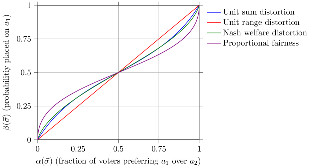
As there are only two possible rankings over two alternatives, we can summarize a preference profile by a real number , which denotes the fraction of agents who prefer to ; then, the remaining fraction of agents prefer to . Similarly, the outcome of a voting rule on a preference profile can also be viewed as a real number which is the probability placed on . We will adapt our notation accordingly throughout this section.
We can disregard the extreme cases where because in such cases, one alternative is preferred by all agents ( if and if ); the voting rule should clearly choose that alternative as it achieves the optimal distortion of with respect to all our welfare functions and utility classes as well as the optimal -proportional fairness.
E.1 Distortion With Unit-Sum Utilities
Given a preference profile , let be the voting rule that selects . We show that this rule always returns the instance optimal distribution minimizing .
Theorem E.1.
For alternatives, and for any preference profile , the voting rule selects a distribution minimizing .
The rule achieves distortion , which is the best possible among all voting rules.
Proof.
Fix a preference profile . Let us write and let
be the best achievable distortion on profile with unit-sum utilities. Then,
| (13) |
Worst-case utilities.
In (13), let us analyze the worst-case utility profile for the term with the numerator . Using the fact that (by the unit-sum assumption), the expression of interest in (13) is
which is maximized when is maximized. To obtain the highest utilitarian welfare for , the fraction of agents who rank first must have and the remaining fraction of agents who rank second must have . Similarly, the worst-case utility profile for the term with the numerator is achieved when the fraction of agents who rank second have and the remaining fraction of agents who rank first have . Therefore, (13) becomes
The left term in the maximum is decreasing in while the right term is increasing. Hence, the maximum of the two is minimized when the two terms become equal, i.e.,
The solution to the equation above is precisely the selected by , proving that it returns the distribution with the best possible distortion on all profiles. Further, at this value of , the distortion achieved is , which is attained at (for which the optimal is also ). ∎
From Section 3, we know that, with alternatives, the optimal distortion with respect to utilitarian welfare and unit-sum utilities is , where the constant hidden in the asymptotic notation lies in . Interestingly, Theorem E.1 shows that the optimal distortion for is , leading one to wonder whether the constant is (close to) the true constant for this problem.
E.2 Distortion With Unit-Range Utilities
Given a preference profile , let be the voting rule that selects .
Theorem E.2.
For alternatives, and for any preference profile , the voting rule selects a distribution minimizing .
The rule achieves distortion , which is the best possible among all voting rules.
Proof.
Fix a preference profile . Let us write , and let
be the best achievable distortion on profile with unit-range utilities. Then, as in the proof of Theorem E.1, we have
| (14) |
Worst-case utilities.
The only difference compared to the proof of Theorem E.1 is the analysis of the worst-case utility profiles in the two expressions inside the maximum in (14). By Lemma A.1, we know that the worst-case utility profile is an approval utility profile. All agents approve their first-ranked alternative and the only question is whether they also approve their second-ranked alternative.
Consider the first term inside the maximum in (14) with in the numerator. We want to find the utility profile that maximizes this term. For the fraction of agents who rank above , we can assume w.l.o.g. that as it can only increase this term. For the rest of the agents that rank above , we know . Hence, . Given this fixed value of , note that
is increasing in . Hence, the term is maximized when is the highest, meaning that the agents who rank above also approve .
Similarly, for the term in (14) with in the numerator, the worst-case utility profile is as follows: fraction of agents who rank first have and the remaining fraction of agents who rank first have . Therefore, (14) becomes
The left term in the maximum is decreasing in while the right term is increasing. Hence, the maximum of the two terms is minimized when the two terms are equal, which yields . This proves that returns the distribution with the best possible distortion on all profiles. Further, at this value of , the distortion achieved is , which is attained at . ∎
E.3 Distortion With Respect to Nash Welfare
Given a preference profile , let be the voting rule that selects where . This is well-defined since since is strictly increasing and invertible.
Theorem E.3.
For alternatives, and for any preference profile , the voting rule selects a distribution minimizing , the distortion with respect to Nash welfare.
The rule achieves distortion with respect to Nash welfare, which is the best possible among all voting rules.
Proof.
Fix a preference profile . Write , and let be the best achievable distortion on the profile . Note that
| (15) |
Reduction to approval utilities.
From Lemma A.3, we know that the worst case for distortion with respect to Nash welfare is achieved at an approval utility profile. Under an approval utility profile , the fraction of agents who prefer to have equal to or , and the remaining fraction of agents have equal to or . If an agent approves both alternatives, then regardless of and . Based on these observations, we can rewrite from (15) as
Finding the optimal distribution.
If , then and the inner expression evaluates to , which is maximized at . Similarly, when , the inner expression evaluates to , which is maximized at . Therefore, we have
This is minimized when , and the unique minimizer of this expression is precisely the selected by . This proves that always returns the distribution with the best possible distortion with respect to the Nash welfare on all profiles. Further, at this , the distortion achieved is , which is attained at (for which the optimal is also ). ∎
E.4 Proportional Fairness
Given a preference profile , let be the voting rule that selects .
Theorem E.4.
For alternatives, and for any preference profile , the voting rule selects a distribution minimizing .
The rule is -proportionally fair, which is the best possible among all voting rules.
Proof.
Fix a preference profile . Let us write and let . From Lemma 4.1, we have
This expression is minimized when
which precisely yields the satisfying returned by . This shows that always returns the distribution with the best possible proportional fairness on profile . Further, at this value of , the proportional fairness achieved is , which is attained at (for which the optimal is also ). ∎