Propagation of spin channel waves

Abstract

A mutilated model is constructed to approximate the collision term of spin Boltzmann equation that incorporates newly appearing collisional invariants i.e, the total angular momentum. With recourse to degenerate perturbation theory, the dispersion relations of hydrodynamic modes are formulated, among which spin modes are responsible for spin equilibration. We find that the non-locality does not change the sound speed but slows down the propagation of spin channel waves. The damping rates of spin modes are close to those of spinless modes over a reasonable parameter value range. The results reveal that both spin and momentum should be treated simultaneously in a unified transport framework. In the nonrelativistic limit, the short-wavelength behavior for normal modes is also explored and there exists a critical point for every distinct discrete mode over which only quasiparticle modes contribute.

I Introduction

The experimental developments in measuring the spin-related observables of $\Lambda$ hyperons [1, 2, 3, 4] have raised extensive interests in global polarization [5, 6, 7, 8, 9, 10, 11, 12, 13] and local polarization [14, 15]. Theoretical calculations are not consistent with experiment results in local polarization, which is referred to as “spin sign problem” and originates from the fact that spin does not reach equilibrium as expected, see [16] for a recent review. In the past few years, different efforts are made to get insight into the spin puzzle along the line of spin hydrodynamics [17, 18, 19, 20, 21, 22, 23, 24, 25, 26, 27, 28, 29], and quantum kinetic theory [30, 31, 32, 33, 34, 35, 36], among which spin relaxation becomes essential because the relaxation rate of the spin density toward its equilibrium value is crucial in determining how the spin polarization evolves in time in theoretical simulations of QCD plasma.

When we talk about spin equilibration of a spinful system, there is a increase of degrees of freedom compared to a spinless system. Considering a collection of quasi-particles with nonzero spins, the dynamic variables are necessarily enlarged to include another particle property spin, i.e, the distribution function for describing the system made of quasi-particles has dependence on spin. From a more general view irrespective of quasi-particle picture, the evolution functions turn out to be conservation laws $\partial_{\mu}T^{\mu\nu}=0,\,\partial_{\lambda}\Sigma^{\lambda\mu\nu}=0$ where $T$ and $\Sigma$ denote the energy momentum tensor and total angular momentum tensor. Canonically, we allow a division $\Sigma^{\mu\alpha\beta}\equiv(x^{\alpha}T^{\mu\beta}-x^{\beta}T^{\mu\alpha})+S^{\mu\alpha\beta}$, where $x$ is the space-time coordinate and $S^{\mu\alpha\beta}=-S^{\mu\beta\alpha}$ is newly defined spin tensor. In this context, the local equilibrium state is defined as the state with maximum local entropy or vanishing divergence of local entropy four-current. For a spinful system, the entropy current receives the contribution from spin tensor, which is exactly reflected in the form of statistical operator [37, 23, 28].

Similar to the still unsettled question of how thermal equilibrium in relativistic heavy-ion collisions is reached, the questions of how the spin of quarks relaxes to equilibrium and whether it equilibrates faster than momentum or not remain under debates. Note that there have been many efforts exploring the spin relaxation rate including but not limited to perturbative QCD techniques [38, 39, 40, 41], the Nambu–Jona- Lasinio model [42], the AdS/CFT correspondence [43], an effective vertex for the interaction with the thermal vorticity [44, 45] and a second-order spin hydrodynamic calculation [29]. When spin is considered, one must take into account the conservation of total angular momentum in hydrodynamic description especially for a system with considerable spin-orbit conversion due to frequent interactions. Accompanied by newly introduced degrees of freedom, there arises new physical phenomenon of the propagation of spin channel waves. Analogous to sound propagation in spinless (spin-averaged) fluids [46], the propagation of spin channel waves should be also fundamental in spin hydrodynamic theory and deserve a comprehensive exploration, which we expect to provide in this work.

As with the recent studies [47, 41, 26], we focus on a linear mode analysis in the current work and find that spin relaxation couples to the attenuation of spin modes. Therefore, spin relaxation time is identified as the lifetime of spin modes, based on which one can make a direct comparison of two typical time scales in relation with spin and momentum relaxation. On the other hand, the researches on spin polarization directly promotes the developments of spin kinetic theory. Once spin is considered, there also arises new physical phenomenon of the propagation of spin channel waves. Analogous to sound propagation in ordinary fluids, the propagation of spin channel waves should be also fundamental in spin hydrodynamic theory.

This paper is organized as follows. In Sec. II we show how to construct the mutilated collision term incorporating six new collision invariants introduced by spin Boltzmann equation [30]. In Sec. III we adopt the method of degenerate perturbation theory widely used in quantum mechanics to derive the dispersion relations of discrete normal modes up to second order in wavenumbers where the discussion of spin relaxation is also presented. After that, the comparison with other associated research works is given in Sec. IV. In Sec. V, we talk about the short wavelength behavior of those normal modes. Summary and outlook are given in Sec. VI. Natural units $k_{B}=c=\hbar=1$ are used. The metric tensor is given by $g^{\mu\nu}=\operatorname{diag}(1,-1,-1,-1)$ , while $\Delta^{\mu\nu}\equiv g^{\mu\nu}-u^{\mu}u^{\nu}$ is the projection tensor orthogonal to the four-vector fluid velocity $u^{\mu}$ and $\epsilon^{\mu\nu\alpha\beta}$ is Levicivita tensor. In addition, we employ the antisymmetric shorthand, $X^{[\mu\nu]}\equiv(X^{\mu\nu}-X^{\nu\mu})/2.$

II Mutilated collision operator

When it comes to spin-induced phenomena, the framework of transport theory must be extended to incorporate the information of spin evolution. To that end, the spin Boltzmann equation for massive spin-$1/2$ fermions with non-local collision effects was proposed, where the consistent interpretation for equilibrium state and collision invariants is elaborated [30].

Here we choose to work out the propagation of hydrodynamic modes by constructing a mutilated collision operator based on the collision invariants appearing in [30] instead of directly solving the complicated linearized integral equation derived in [26]. Note that the collision invariants are exactly eigenfunctions of linearized collision operator with zero as eigenvalues. If insisting on semipositive definiteness and self-adjointness of a linearized collision operator, we are led to treat it as an evolution Hamiltonian operator [26]

$$p\cdot\partial\chi(x,p,\bm{s})=-L\chi(x,p,\bm{s}),$$ (1)

where we assume that there is no external field in the above linearized transport equation. In addition, $\chi(x,p,\bm{s})$ represents the deviation function from equilibrium distribution dependent on space-time coordination $x$, particle momentum $p$ and spin $\bm{s}$, and $L$ denotes the linearized collision operator with its explicit form temporarily uncovered.

Under homogeneous circumstance, Eq.(1) can be formally solved and the resulting solution is

$$\chi(t,p,\bm{s})=\exp(-\frac{L}{u\cdot p}t)\chi(p,\bm{s}),$$ (2)

with the initial condition $\chi(t=0,p,\bm{s})=\chi(p,\bm{s})$.

According to Hamiltonian formalism, we can always expand the deviation function as a sum of linear superposition of the eigen states of linearized collision operator $L$. As time goes by, zero modes can survive long time while positive ones become damped exponentially and less dominant. Hereafter, we concentrate on the zero modes and see how they respond to the perturbation of non-uniformity, namely, the space coordination dependence of deviation function $\chi(x,p,\bm{s})$ is recovered.

The linearized collision operator $L$ is now approximated by a mutilated operator

$$-L\sim\big{(}-\gamma+\gamma\sum_{n=1}^{11}|\lambda_{n}\rangle\langle\lambda_{n}|\big{)}$$ (3)

with $|\lambda_{n}\rangle$ being orthonormal eigenfunctions of $L$ and $\gamma$ being a representative positive eigenvalue. One can easily verify that $L$ inherit basic properties of what we require for a linearized collision operator such as semipositive definiteness, self-adjointness and $L|\lambda_{n}\rangle=0,n=1,\cdots 11$ and $L|\lambda_{n}\rangle=\gamma|\lambda_{n}\rangle,n>11$. Here the “mutilated” means all positive eigenvalues collapse into one chosen positive eigenvalue (it is suggestive to take the smallest one). The zero modes with eleven-fold degeneracy exactly correspond to collision invariants $1,p^{\mu}$ and $J^{\mu\nu}$, where the identification of $J^{\mu\nu}\equiv 2\Delta^{[\mu}p^{\nu]}+\frac{1}{2}\Sigma^{\mu\nu}_{\bm{s}}$ as total angular momentum is seen in [30, 31] with

$$\Delta^{\mu}\equiv-\frac{1}{2m(p\cdot\hat{t}+m)}\,\epsilon^{\mu\nu\alpha\beta}p_{\nu}\hat{t}_{\alpha}\bm{s}_{\beta}$$ (4)

characterizing the non-locality in a collision, where $\hat{t}^{\mu}$ is the time-like unit vector which is $(1,\boldsymbol{0})$ in the frame where $p^{\mu}$ is measured.

It may be observed that this is exactly a kind of relaxation time approximation (RTA) by identifying $\gamma$ with the reciprocal of relaxation time $\tau_{R}^{-1}$. Compared to traditional RTA, the novel RTA or mutilated operator is proved to reconcile the momentum dependence of the relaxation time with the macroscopic conservation laws. When the relaxation time has no momentum dependence, one can always argue that RTA is consistent with the conservation laws by imposing matching conditions but this is not the general case. Without elaboration, we refer to a recent letter [48]. From now on, $\gamma$ is parameterized as energy dependent $\gamma\equiv\gamma_{R}/\tau^{\lambda}$ with an energy-independent constant $\gamma_{R}$.

In order to seek a solution of the form, $\chi\sim\tilde{\chi}e^{-ik\cdot x}$, we substitute it into Eq.(1),

$$\tau\omega\tilde{\chi}+\hat{p}^{\mu}l_{\mu}\kappa\tilde{\chi}=-iL\tilde{\chi},$$ (5)

where the linearized collision operator is put less abstract with the specified form shown as

$$L\tilde{\chi}\equiv\gamma\tau\big{(}\tilde{\chi}-\sum_{n=1}^{11}(\tilde{\psi}_{n},\tau\tilde{\chi})\tilde{\psi}_{n}\;\big{)},$$ (6)

with notations $\tau\equiv\frac{p\cdot u}{T},\hat{p}\equiv\frac{p}{T}$. Here we introduce dimensionless frequency and wave vector

$$\omega\equiv\frac{u\cdot k}{n\sigma},\quad\kappa^{\alpha}\equiv\frac{\Delta^{\alpha\beta}k_{\beta}}{n\sigma},$$ (7)

and one unit vector

$$l^{\alpha}\equiv\frac{\kappa^{\alpha}}{\kappa},\quad\kappa\equiv\sqrt{-\kappa\cdot\kappa},$$ (8)

where $n$ is density, $T$ is temperature and $\sigma$ is an arbitrary constant with the dimension of cross sections. Additionally, the inner product is defined as

$$(B,C)=\frac{1}{(2\pi)^{3}}\int d\Gamma\exp(-\beta\cdot p)B(p,\bm{s})C(p,\bm{s}),$$ (9)

with the measure defined as $d\Gamma\equiv d^{4}p\,\delta(p^{2}-m^{2})\sqrt{\frac{p^{2}}{3\pi^{2}}}d^{4}\bm{s}\,\delta(\bm{s}\cdot\bm{s}+3)\delta(p\cdot\bm{s})$ [20], and the eigenfunctions $|\lambda_{n}\rangle$ are also replaced by less-abstract functions $\tilde{\psi}_{n}$ given by

$$\tilde{\psi}_{1}=\frac{1}{\sqrt{V^{(0)}_{1,1}}},\quad\tilde{\psi}_{2}=\beta\frac{u\cdot p-\frac{I_{20}}{I_{10}}}{\sqrt{V^{(0)}_{2,2}}},\quad\tilde{\psi}_{3}=\frac{\beta l\cdot p}{\sqrt{V^{(0)}_{3,3}}},$$

$$\tilde{\psi}_{4}=\frac{\beta j\cdot p}{\sqrt{V^{(0)}_{3,3}}},\quad\tilde{\psi}_{5}=\frac{\beta v\cdot p}{\sqrt{V^{(0)}_{3,3}}},\quad\tilde{\psi}_{6}=\frac{u_{\mu}J^{\mu\nu}l_{\nu}}{\sqrt{V^{(0)}_{6,6}}},$$

$$\tilde{\psi}_{7}=\frac{u_{\mu}J^{\mu\nu}j_{\nu}}{\sqrt{V^{(0)}_{6,6}}},\quad\tilde{\psi}_{8}=\frac{u_{\mu}J^{\mu\nu}h_{\nu}}{\sqrt{V^{(0)}_{6,6}}},\quad\tilde{\psi}_{9}=\frac{l_{\mu}J^{\mu\nu}j_{\nu}}{\sqrt{V^{(0)}_{9,9}}},$$

$$\tilde{\psi}_{10}=\frac{l_{\mu}J^{\mu\nu}h_{\nu}}{\sqrt{V^{(0)}_{9,9}}},\quad\tilde{\psi}_{11}=\frac{j_{\mu}J^{\mu\nu}h_{\nu}}{\sqrt{V^{(0)}_{9,9}}},$$ (10)

where

$$I_{nq} \equiv\frac{2}{(2q+1)!!}\int\frac{\rm d^{4}p}{(2\pi)^{3}}\,\delta(p^{2}-m^{2})(u\cdot p)^{n-2q},$$ (11)

$$V^{(\lambda)}_{i,j} \equiv\beta\int\frac{\rm d\Gamma}{(2\pi)^{3}}\tau^{\lambda}\tilde{\psi}_{i}\kappa\cdot p\,\tilde{\psi}_{j}\exp(-\beta\cdot p).$$ (12)

Here $\beta^{\mu}\equiv\beta u^{\mu}=\frac{u^{\mu}}{T}$ and we introduced two auxiliary unit vectors $j,h$ to form an orthonormal triad with $u$ and $l$. In the remainder of this work, a quiescent background fluid i.e., $u^{\mu}=(1,0,0,0)$ is chosen, then the triad $(u,j,h,l)$ stands for the projection to the directions of $(t,x,y,z)$. Last but not the least, note the eigenfunctions Eq.(II) has been defined to fulfill the orthonormal condition

$$(\tilde{\psi}_{\alpha},\tau\tilde{\psi}_{\beta})=\delta_{\alpha\beta}.$$ (13)

III Degenerate perturbation theory

As a familiar problem in the perturbation theory, the solutions to Eq.(5) can be sought in the fashion as used in quantum mechanics by treating the spatial term $\hat{p}^{\mu}\kappa_{\mu}\tilde{\chi}$ as a perturbation with respect to $-iL\tilde{\chi}$, then the eigenfunctions and eigenvalues can be routinely expanded into

$$\tilde{\chi}=\tilde{\chi}^{(0)}+\tilde{\chi}^{(1)}+\cdots,$$

$$\omega=\omega^{(0)}+\omega^{(1)}+\omega^{(2)}+\cdots.$$ (14)

The dispersion relations, which are obtained from the secular equation for Eq.(5), are formulated up to first order in $\kappa$ [26]

$$\omega^{(1)}_{1}=-\omega^{(1)}_{2}=\sqrt{H^{(0)2}_{2,3}+H^{(0)2}_{1,3}}$$

$$\omega^{(1)}_{3}=\omega^{(1)}_{4}=\omega^{(1)}_{5}=\omega^{(1)}_{6}=\omega^{(1)}_{11}=0,$$

$$\omega^{(1)}_{7}=\omega^{(1)}_{8}=H^{(0)}_{7,9},\quad\omega^{(1)}_{9}=\omega^{(1)}_{10}=-H^{(0)}_{7,9},$$ (15)

where

$$H^{(\lambda)}_{i,j}\equiv\beta\int\frac{\rm d\Gamma}{(2\pi)^{3}}\tau^{\lambda}\tilde{\psi}_{i}\kappa\cdot p\,\tilde{\psi}_{j}\exp(-\beta\cdot p).$$ (16)

One can readily verify that the results of the first five spinless modes are the same as those in [46] independent of the details of interactions involved. At the meantime, we find that only four transverse spin modes ($\omega_{7},\omega_{8},\omega_{9},\omega_{10}$) are propagating with the same speed of propagation $c_{\text{spin}}=\omega^{(1)}_{7}/\kappa$ where the minus sign represents the opposite traveling direction. The dependence of propagating velocity of discrete normal modes on the reduced mass $z$ ($z\equiv\beta m$) is exhibited in Fig.1. As a comparison, we also exhibit the sound speed $c_{s}=\omega^{(1)}_{1}/\kappa$, which is larger than $c_{\text{spin}}$. In addition, $c_{\text{spin}}$ under the condition of spin angular momentum conservation (SAC) is shown by the solid black line. When setting the non-locality $\Delta$ zero, $c_{\text{spin}}$ returns to $c_{\text{spin}}|_{\text{SAC}}$ that is also presented in [49].

It can be seen clearly from Fig.1 that the propagating speeds of sound modes and transverse spin modes are monotonically decreasing functions of $z$ and the inclusion of non-locality in collisions will slow down the propagation of spin channel waves (we call them spin channel waves in analogy with sound waves), while the propagation of sound wave is immune to that change. The non-locality does not alter the equation of state (EOS) in contrast to Enskog-type non-locality with hard-sphere exclusion potential. A quick inspection shows that $1$ and $p^{\mu}$ are not collision invariants of Enskog collision term any more and the redefinition or modification to the static pressure is needed to retain the form of conservation laws [50].

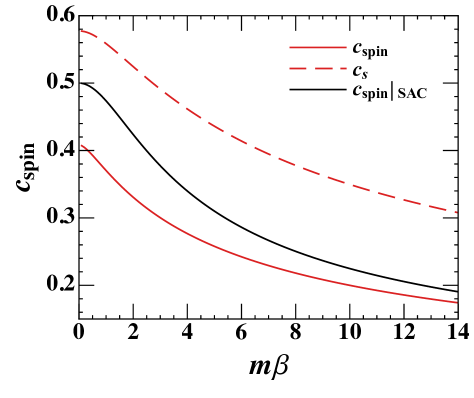
Figure 1: The propagating speed of discrete normal modes as a function of $\beta m$.

Up to the second order in $\kappa$, the dispersion relations or frequencies are summarized as

$$\omega_{1}=c_{s}\kappa-i\Gamma_{1},\quad\omega_{2}=-c_{s}\kappa-i\Gamma_{1},$$

$$\omega_{3}=-i\Gamma_{3},\quad\omega_{4}=\omega_{5}=-i\Gamma_{4},\quad$$

$$\omega_{6}=-i\Gamma_{6},\quad\omega_{7}=\omega_{8}=c_{\text{spin}}\kappa-i\Gamma_{7},$$

$$\omega_{9}=\omega_{10}=-c_{\text{spin}}\kappa-i\Gamma_{7},\quad\omega_{11}=-i\Gamma_{11},$$ (17)

with the damping coefficients defined as

$$\Gamma_{1} \equiv\frac{1}{\gamma_{R}}\Big{[}Q^{(\lambda)}_{1,1}+\frac{1}{2}\omega^{(1)2}_{1}\big{(}\frac{H^{(0)2}_{1,3}}{\omega^{(1)2}_{1}}\frac{V^{(\lambda)}_{1,1}}{V^{(0)}_{1,1}}+\frac{H^{(0)2}_{2,3}}{\omega^{(1)2}_{1}}\frac{V^{(\lambda)}_{2,2}}{V^{(0)}_{2,2}}$$

$$+\frac{V^{(\lambda)}_{3,3}}{V^{(0)}_{3,3}}+\frac{2H^{(0)}_{1,3}H^{(0)}_{2,3}V^{(\lambda)}_{1,2}}{\omega^{(1)2}_{1}\sqrt{V^{(0)}_{11}V^{(0)}_{2,2}}}\big{)}-2\omega^{(1)}_{1}\big{(}\frac{H^{(0)}_{1,3}}{\omega^{(1)}_{1}}H^{(\lambda)}_{1,3}$$

$$+\frac{H^{(0)}_{2,3}}{\omega^{(1)}_{1}}H^{(\lambda)}_{2,3}\big{)}\Big{]},$$

$$\Gamma_{3} \equiv\frac{1}{\gamma_{R}}Q^{(\lambda)}_{3,3},\quad\Gamma_{4}\equiv\frac{1}{\gamma_{R}}Q^{(\lambda)}_{4,4},\quad\Gamma_{6}\equiv\frac{1}{\gamma_{R}}Q^{(\lambda)}_{6,6},$$

$$\Gamma_{7} \equiv\frac{1}{\gamma_{R}}\big{[}Q^{(\lambda)}_{7,7}+\frac{1}{2}H^{(0)2}_{7,9}\big{(}\frac{V^{(\lambda)}_{6,6}}{V^{(0)}_{6,6}}+\frac{V^{(\lambda)}_{9,9}}{V^{(0)}_{9,9}}\big{)}-2H^{(0)}_{7,9}H^{(\lambda)}_{7,9}\,\big{]},$$

$$\Gamma_{11} \equiv\frac{1}{\gamma_{R}}Q^{(\lambda)}_{11,11},$$ (18)

where

$$Q^{(\lambda)}_{i,j} =\beta\int\frac{\rm d\Gamma}{(2\pi)^{3}}\tilde{\chi}_{i}\frac{\tau^{\lambda}(p\cdot\kappa)^{2}}{p\cdot u}\tilde{\chi}_{j}\exp(-\beta\cdot p),$$ (19)

and $\tilde{\chi}_{i}$’s are given in Eq.(52) of [26].

Then all the damping rates are shown in Fig.2 as functions of reduced mass $z$,

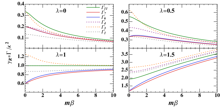
Figure 2: The damping coefficients of discrete normal modes as functions of $\beta m$. The spin modes are denoted by solid lines while the spinless modes are denoted by dashed lines

which are crucial because the attenuation of spin modes couples to the dissipation of spin density [26] while other spinless modes are not responsible for it. Among the spin modes four propagating transverse modes are degenerate in the damping rates $\Gamma_{7}$, while the other two are non-propagating longitudinal modes which are purely decaying at their respective decaying rates $\Gamma_{6}$ and $\Gamma_{11}$. One can clearly see that the choice of $\lambda$ dramatically affects the attenuation of these discrete normal modes both in magnitude and in their dependence on reduced mass $z$.

The specific value of $\lambda$ relies on the dynamic details and corresponds to various physical scenarios. For example, $\lambda=0$ corresponds to traditional RTA proposed firstly by Anderson and Witting (AW) [51], while $\lambda=0.5$ is argued to well approximate the effective kinetic descriptions of quantum chromodynamics [48, 52, 53, 54]. When $\lambda$ is big enough (see $\lambda=1.5$) and may be out of realistic range $0\lesssim\lambda\lesssim 1$, the tendency even flips compared to AW case, all damping coefficients are monotonically increasing functions of $z$, and the spin modes are separated from spinless ones forming the hierarchy of $\Gamma_{\text{spin}}\lesssim\,\Gamma_{\text{nonspin}}$. On the other hand, when $\lambda$ is comparatively small $\lambda=0$ or corresponds to relevant QCD scenario $\lambda=0.5$, the damping is almost as slow as spinless ones, namely, the dynamic evolution of spin and momentum are twisted in this scenario over a wide range of $z$. As a short summary, we find that there is no obvious separation of two different relaxation time scales for discrete normal modes over a relevant value range of $0\lesssim\lambda\lesssim 1$, which reveals the necessity of unified transport of spin and momentum. Therefore, we should treat the evolution of both spin and momentum on the same footing.

IV Compare with other theoretic results

In this section, we provide a detailed comparison of current work with other related researches [49, 21, 47]. They have something in common and also many differences, which can be elaborated in three aspects.

• Framework. In mentioned researched works, the authors all first construct a first-order hydrodynamics based on thermodynamic second-law [21, 47] and AW relaxation time approximation [49]. After that, a linearization around the ideal fluids is made to give the analysis on the hydrodynamic modes. Wheres, one can make it directly via transport equation without recourse to hydrodynamics. Here we take spin Boltzmann equation as the start point and concentrate on the analysis on zero kinetic modes, which forms one-to-one correspondence to hydrodynamic modes in the limit of long wavelength [55]. In this sense, they are commonly called discrete normal modes. However, we have to admit that the current formalism only concerns with what is conserved, i.e, hydrodynamic modes.

• Degrees of freedom. This aspect closely concerns the definition of total angular momentum tensor $J^{\lambda,\mu\nu}$. Note that almost all spin hydrodynamics on the market take the same definition of $J^{\lambda,\mu\nu}$ as what we employ in this paper. Because of the antisymmetry of last two indices, the independent degrees of freedom are six, two longitudinal ones and four transverse ones, which holds no matter what pseudo-gauge specifying the energy-momentum tensor and spin tensor is taken. However, recently in [47], the authors recommend a new definition for $J^{\lambda,\mu\nu}$: $J^{\lambda,\mu\nu}$ is now totally antisymmetric in all indices. Other than widely used traditional definitions, the degrees of freedom reduce to only three, which excludes three degrees of freedom related to boost symmetry.

• The existence of propagating degrees of freedom. The calculations in [49] exactly correspond to the case of $\lambda=0$ where the conservation of spin angular momentum is assumed. If turning off the nonlocality, namely, setting the nonlocal collision shift $\Delta^{\mu}$ zero, our results will return to that of [49]. Protected by the conservation laws, these two works all report that only transverse spin modes propagate similar to the behavior of electromagnetic wave but contrary to longitudinal sound modes. While in related studies [21, 47], the authors concentrate on non-conserved spin density, which is inherently relaxation-type. Therefore, there are no propagating degrees of freedom in spin sector therein. As a supplement, we note that if we naively construct first order theory of spin hydrodynamics via gradients expansion, spin angular momentum is still conserved even if the nonlocality of collisions is taken into account [25], then the linear mode analysis based on hydrodynamic equations does not alter compared with [49]. One should expect something new emanates at the second order.

V The behavior of hydrodynamic modes in nonrelativistic limit

In this section, the existence of spin modes and their behavior outside the range of perturbation are explored. For simplicity, we take the nonrelativistic limit and neglect the energy dependence of $\gamma$. In the nonrelativistic limit $p^{\mu}\rightarrow m(1,\bm{v})$ with the particle three velocity $\bm{v}$, which implies $d\Gamma\rightarrow\frac{m^{2}}{2\sqrt{3}\pi}\int d^{3}vd^{3}\bm{s}\delta(\bm{s}^{2}-3)$, and

$$\sqrt{\frac{z}{2}}(-i\omega\tilde{\chi}+i\bm{\kappa}\cdot\bm{v}\tilde{\chi})=-\gamma\big{(}\tilde{\chi}-\sum_{n=1}^{11}(\tilde{\psi}_{n},\tilde{\chi})\tilde{\psi}_{n}\;\big{)},$$ (20)

where a factor $\sqrt{\frac{z}{2}}$ has been absorbed into $\gamma$ and $\bm{\kappa}=(0,0,\kappa)$ without losing generality, then define fluctuation amplitudes

$$\rho_{n}(\omega,\bm{\kappa})\equiv(\tilde{\psi}_{n},\tilde{\chi}(\omega,\bm{\kappa},p,\bm{s})\,).$$ (21)

Note that the weight function in Eq.(9) is replaced by the equilibrium distribution $f_{0}=(\frac{z}{2\pi})^{\frac{3}{2}}\exp(-\frac{1}{2}zv^{2})$. Introduce $\bm{c}\equiv\sqrt{\frac{z}{2}}\bm{v},\,\bar{c}\equiv\frac{\sqrt{\frac{z}{2}}\omega+i\gamma}{\kappa},\,\hat{\gamma}\equiv\frac{i\gamma}{\kappa}$, and if $\bar{c}$ is not real, we get

$$\tilde{\chi}=\frac{\hat{\gamma}\sum_{n=1}^{11}\rho_{n}\psi_{n}}{\bar{c}-c_{z}},$$ (22)

then these amplitudes can be cast into

$$\rho_{6} =\hat{\gamma}Z(\bar{c})\rho_{6},$$

$$\rho_{7} =\frac{\hat{\gamma}z^{2}}{2}\big{(}\frac{Z(\bar{c})}{z^{2}}(1+2\bar{c}^{2})-\frac{2\bar{c}}{z^{2}}\,\big{)}\rho_{7}+\frac{\hat{\gamma}m}{4\sqrt{V_{9,9}}}$$

$$\times\big{(}\,(2\bar{c}-\frac{2\bar{c}}{z}-\frac{2\bar{c}^{3}}{z})Z(\bar{c})+\frac{3}{z}+\frac{2\bar{c}^{2}}{z}-2\big{)}\rho_{9},$$

$$\rho_{9} =\frac{\hat{\gamma}m}{4\sqrt{V_{9,9}}}\big{(}\,(2\bar{c}-\frac{2\bar{c}}{z}-\frac{2\bar{c}^{3}}{z})Z(\bar{c})+\frac{3}{z}+\frac{2\bar{c}^{2}}{z}$$

$$-2\big{)}\rho_{7}+\frac{\hat{\gamma}m^{2}}{4V_{9,9}}\big{(}\,(\frac{\bar{c}^{4}}{z^{2}}+\frac{3\bar{c}^{2}}{2z^{2}}-\frac{2\bar{c}^{2}}{z}+\frac{1}{z^{2}}-\frac{1}{z}$$

$$+1)Z(\bar{c})-\frac{\bar{c}^{3}}{z^{2}}-\frac{3\bar{c}}{2z^{2}}-\frac{\bar{c}}{2z^{2}}+\frac{2\bar{c}}{z}\big{)}\rho_{9},$$

$$\rho_{11} =\frac{\hat{\gamma}m^{2}}{4V_{9,9}}\big{(}\,(\frac{\bar{c}^{2}}{z^{2}}+\frac{2}{z^{2}}-\frac{2}{z}+1)Z(\bar{c})-\frac{\bar{c}}{z^{2}}\,\big{)}\rho_{11},$$ (23)

with $V_{9,9}\equiv\frac{m^{2}}{4}(1-\frac{2}{z}+\frac{5}{2z^{2}})$, $Z(\bar{c})\equiv\frac{1}{\sqrt{\pi}}\int_{-\infty}^{\infty}dt\exp(-\frac{z}{2}t^{2})\frac{1}{\sqrt{\frac{2}{z}}\bar{c}-t}$ and $(\rho_{8},\rho_{10})$ is just a copy of $(\rho_{7},\rho_{9})$.

The determination of dispersion relations is equivalent to finding roots of

$$\Phi_{1}(\bar{c}) =\hat{\gamma}Z(\bar{c})-1,$$

$$\Phi_{2}(\bar{c},z) =\frac{\hat{\gamma}m^{2}}{4V_{9,9}}\big{(}(\frac{\bar{c}^{2}}{z^{2}}+\frac{2}{z^{2}}-\frac{2}{z}+1)Z(\bar{c})-\frac{\bar{c}}{z^{2}}\big{)}-1,$$

$$\Phi_{3}(\bar{c},z) =\big{[}\frac{\hat{\gamma}z^{2}}{2}\big{(}\frac{Z(\bar{c})}{z^{2}}(1+2\bar{c}^{2})-\frac{2\bar{c}}{z^{2}}\,\big{)}-1\big{]}\big{[}\frac{\hat{\gamma}m^{2}}{4V_{9,9}}$$

$$\times\big{(}\,(\frac{\bar{c}^{4}}{z^{2}}+\frac{3\bar{c}^{2}}{2z^{2}}-\frac{2\bar{c}^{2}}{z}+\frac{1}{z^{2}}-\frac{1}{z}+1)Z(\bar{c})$$

$$-\frac{\bar{c}^{3}}{z^{2}}-\frac{3\bar{c}}{2z^{2}}-\frac{\bar{c}}{2z^{2}}+\frac{2\bar{c}}{z}\big{)}-1\big{]}-\frac{\hat{\gamma}^{2}m^{2}}{16V_{9,9}}$$

$$\times\big{(}\,(2\bar{c}-\frac{2\bar{c}}{z}-\frac{2\bar{c}^{3}}{z})Z(\bar{c})+\frac{3}{z}+\frac{2\bar{c}^{2}}{z}-2\big{)}^{2}.$$ (24)

For illustration we only display how to extract the encoding information from $(\rho_{7},\rho_{9})$, which can be safely extended to other fluctuation amplitudes. it is convenient to invoke the residue theorem that the number of zeros of $\Phi_{3}$ in a region of the complex $\bar{c}$-plane in which $\Phi_{3}$ is an analytic function is equal to the times of the representative point $\Phi_{3}$ in the $\Phi_{3}$-plane encircles the origin. With the asymptotic behavior of $Z(\bar{c})$ for large $|\bar{c}|$ and along the real axis detailedly given in Appendix.A, it is easy to verify that there is a critical value for $\kappa$ below which zeros exist, i.e. the dispersion relations of discrete normal modes hold, which is also known as an onset of hydrodynamic description [56]. When $\kappa$ exceeds the critical value $\kappa_{o}$, there are no discrete modes anymore. The critical value $\kappa_{o}$ for various spin modes are numerically solved and displayed in TABLE. 1.

	L(6th)	L(11th)	T
$\kappa_{o}/n\sigma\gamma$	1.772	1.762$\pm$0.040	1.754$\pm$0.079

Table 1: The critical value $\kappa_{o}$ for longitudinal (L) and transverse (T) spin modes. In the last two columns, $a\pm b$ represents that $a$ is formulated with $z=10$ and $b$ is the maximum discrepancy from $a$ when $z$ ranges from $5$ to $20$.

The results are exact in the nonrelativistic limit.

Several comments are followed in order.

• The present calculation is limited to nonrelativistic situation, but the qualitative behavior of normal mode should be independent of whether we take this limit. As the concept of long or short wavelength concerns only the dynamics, it is thus irrelevant to kinematics. We expect the qualitative behavior of criticality is identical for both relativistic and nonrelativistic cases.

• The existence of the critical behavior of discrete normal modes reflects the transition from collision-dominated region to Knudsen region, though the realistic distinction may not be that clear. In simplified mutilated model, the transition region collapses into a critical point and the short or long wavelength dynamics can be uniformly described without extra changes.

• Discrete normal modes including spin modes are exactly the ways of ordered particle collective motion organized by collisions. In long wavelength limit, they return to zero modes. In free-flow dominated region, the initial fluctuation is carried away by disordered particles. Thus no discrete modes and dispersion relations are found, which happens while $\kappa$ exceeds $\kappa_{o}$. There is an exception that $\bar{c}$ is real . The behavior of normal modes when $\bar{c}$ is real is alike to that in Knudsen region. Two cases are deeply connected with each other by verifying that the fluctuation $\tilde{\chi}$ in both situations takes the form of single particle continuum spectrum see Appendix.B for details. It makes sense that in the case of long wavelength there are hydrodynamic modes and quasiparticle modes and only quasiparticle modes are left in Knudsen region.

• As a supplement, the critical $\kappa_{o}$’s for two sound modes, two shear modes, and one heat mode are $1.853,1.772$ and $1.918$ respectively [57]. Thus there exists an another hierarchy $\kappa_{o,\text{spin}}\lesssim\kappa_{o,\text{non}}$, which manifests that discrete spinless modes are more resistant to the “destruction” of non-uniformity. Nevertheless, this discrepancy is negligible.

VI Summary and outlook

In this paper, we constructed a mutilated model incorporating the collisional invariants in spin Boltzmann equation, where six new zero modes associated with total angular momentum arise from nontrivial dynamics of nonlocal collisions. The dispersion relations of all discrete normal modes, namely, the propagating speeds and attenuation rates are all computed up to second order perturbation. At the first order perturbation in spatial non-uniformity, the non-locality contributes nothing to sound speed but slows down the propagation of spin channel waves. At the second order perturbation, the damping rates of spin modes are close to those of spinless modes for various relevant energy dependence of $\gamma$. The results reveal that spin and momentum relax at comparable damping rates parameterized for modeling realistic physical scenarios and a unified transportation of both spin and momentum is necessary. In the nonrelativistic limit, we investigate the existence conditions for discrete normal modes and find there exists a critical point for every distinct discrete mode over which only quasiparticle modes contribute.

There are possible extensions to the current work. The first extension lies in a more accurate extraction of parameter $\gamma$ or the reciprocal of relaxation time in RTA. Generally speaking, $\gamma$ is not a free parameter and can be in principle solved from spin Boltzmann equation consistently though it might be complicated to evaluate nonzero eigenvalues and corresponding eigenfunctions of the full linearized collision operator. Secondly, our analysis bases itself on the spin Boltzmann equation specialized to the collisions between massive spin-$1/2$ fermions. Therefore, our estimation of the relaxation time scales for both spin and momentum transport overlooks other relevant processes such as the collisions between massive quark and gluons or massless $u$ and $d$ quarks. It is likely that these scatterings shall play a big role because the rotating media should carry a large amount of orbital angular momentum yielded by non-central nuclear collisions and thus the components, massless $u$ and $d$ quarks and gluons inevitably polarize or possess considerable orbital angular momentum. Consequently, gluons and light $u,$ $d$ quarks are important sources of the polarization of strange quarks as a result of their mutual interactions.

This work was supported by the NSFC Grant No.11890710, No.11890712 and No.12035006.

Appendix A The asymptotic behavior of $Z(\bar{c})$

In Sec. V, we have introduced an auxiliary function $Z(\bar{c})$ and its asymptotic behavior is crucial to the discussion therein. First we note

$$Z(\bar{c})\equiv \frac{1}{\sqrt{\pi}}\int_{-\infty}^{\infty}dt\exp(-\frac{z}{2}t^{2})\frac{1}{\sqrt{\frac{2}{z}}\bar{c}-t}$$

$$= \frac{1}{\sqrt{\pi}}\int_{-\infty}^{\infty}d(\sqrt{\frac{z}{2}}t)\exp(-\frac{z}{2}t^{2})\frac{1}{\bar{c}-\sqrt{\frac{z}{2}}t}$$

$$= \frac{1}{\sqrt{\pi}}\int_{-\infty}^{\infty}dt\exp(-t^{2})\frac{1}{\bar{c}-t}.$$ (25)

For large $|\bar{c}|$, the asymptotic behavior of $Z(\bar{c})$ is

$$Z(\bar{c})\sim\sum_{n=0}^{\infty}\frac{\Gamma(n+\frac{1}{2})}{\Gamma(\frac{1}{2})}(\bar{c})^{-2n-1},$$ (26)

which can be derived by expanding Eq.(A) in powers of $\bar{c}$ and the behavior of $Z$ along the real axis is given by

$$\lim\limits_{\epsilon\rightarrow 0}Z(x\pm i\epsilon)=Y(x)\mp i\sqrt{\pi}\exp(-x^{2})$$ (27)

with $Y(x)$ shown as a Dawson integral

$$Y(x)=\frac{1}{\sqrt{\pi}}\text{P}\int_{-\infty}^{\infty}dt\,e^{-t^{2}}\frac{1}{x-t}=2e^{-x^{2}}\int_{0}^{x}dt\,e^{t^{2}},$$ (28)

where $\rm{P}$ denotes the Cauchy principal value.

Appendix B continuum spectrum

When $\bar{c}$ is real, Eq. (22) can not naively be obtained by division. The formal solution should take the form by noticing $x\delta(x)=0$,

$$\tilde{\chi}(\omega,\bm{k})=\frac{1}{m}A(\omega,\bm{k})\delta(\bar{c}-c_{z})+\hat{\gamma}\rm{P}\frac{\sum_{n=6}^{11}\rho_{n}\psi_{n}}{\bar{c}-c_{z}},$$ (29)

where $\rm{P}$ denotes the Cauchy principal value.

Defining $\bar{A}_{\beta}(\omega,\bm{k})\equiv\frac{1}{2\sqrt{3}\pi}\int d^{3}\bm{s}\delta(\bm{s}^{2}-3)A(\omega,\bm{k},\bm{s})\bm{s}_{\beta}$ and various fluctuation amplitudes can be expressed in terms of two parts, i.e., $\rho_{i}=\rho_{i}^{(0)}+\rho_{i}^{(1)}$,

$$\rho^{(1)}_{6} =\frac{1}{m\sqrt{V_{6,6}}}(\frac{z}{2\pi})^{\frac{3}{2}}\int d\Gamma\exp(-\frac{z}{2}v^{2})J^{0z}A(\omega,\bm{k},\bm{s})\delta(\bar{c}-c_{z})=0,$$

$$\rho_{7}^{(1)} =\frac{1}{m\sqrt{V_{6,6}}}(\frac{z}{2\pi})^{\frac{3}{2}}\int d\Gamma\exp(-\frac{z}{2}v^{2})J^{0x}A(\omega,\bm{k},\bm{s})\delta(\bar{c}-c_{z})$$

$$=\frac{1}{8\sqrt{\pi}}\bar{A}_{y}\bar{c}\exp(-\bar{c}^{2}),$$

$$\rho_{9}^{(1)} =\frac{1}{m\sqrt{V^{(0)}_{9,9}}}(\frac{z}{2\pi})^{\frac{3}{2}}\int d\Gamma\exp(-\frac{z}{2}v^{2})J^{zx}A(\omega,\bm{k},\bm{s})\delta(\bar{c}-c_{z})$$

$$=\frac{m}{2\pi^{\frac{1}{2}}\sqrt{V^{(0)}_{9,9}}}(1-\frac{\bar{c}^{2}}{z}-\frac{1}{z})\exp(-\bar{c}^{2})\bar{A}_{y}$$

$$\rho^{(1)}_{11} =\frac{1}{m\sqrt{V^{(0)}_{9,9}}}(\frac{z}{2\pi})^{\frac{3}{2}}\int d\Gamma\exp(-\frac{z}{2}v^{2})J^{xy}A(\omega,\bm{k},\bm{s})\delta(\bar{c}-c_{z})$$

$$=\frac{m}{2\pi^{\frac{1}{2}}\sqrt{V^{(0)}_{9,9}}}(1-\frac{1}{z})\exp(-\bar{c}^{2})\bar{A}_{z}$$

and

$$\rho^{(0)}_{6} =\hat{\gamma}Y(\bar{c})\rho_{6},$$

$$\rho^{(0)}_{7} =\frac{\hat{\gamma}z^{2}}{2}\big{(}\frac{Y(\bar{c})}{z^{2}}(1+2\bar{c}^{2})-\frac{2\bar{c}}{z^{2}}\,\big{)}\rho_{7}+\frac{\hat{\gamma}m}{4\sqrt{V^{(0)}_{9,9}}}\big{(}\,(2\bar{c}-\frac{2\bar{c}}{z}-\frac{2\bar{c}^{3}}{z})Y(\bar{c})+\frac{3}{z}+\frac{2\bar{c}^{2}}{z}-2\big{)}\rho_{9},$$

$$\rho^{(0)}_{9} =\frac{\hat{\gamma}m}{4\sqrt{V^{(0)}_{9,9}}}\big{(}\,(2\bar{c}-\frac{2\bar{c}}{z}-\frac{2\bar{c}^{3}}{z})Y(\bar{c})+\frac{3}{z}+\frac{2\bar{c}^{2}}{z}-2\big{)}\rho_{7}+\frac{\hat{\gamma}m^{2}}{4V^{(0)}_{9,9}}\big{(}\,(\frac{\bar{c}^{4}}{z^{2}}+\frac{3\bar{c}^{2}}{2z^{2}}-\frac{2\bar{c}^{2}}{z}+\frac{1}{z^{2}}-\frac{1}{z}$$

$$+1)Y(\bar{c})-\frac{\bar{c}^{3}}{z^{2}}-\frac{3\bar{c}}{2z^{2}}-\frac{\bar{c}}{2z^{2}}+\frac{2\bar{c}}{z}\big{)}\rho_{9},$$

$$\rho^{(0)}_{11} =\frac{\hat{\gamma}m^{2}}{4V^{(0)}_{9,9}}\big{(}\,(\frac{\bar{c}^{2}}{z^{2}}+\frac{2}{z^{2}}-\frac{2}{z}+1)Y(\bar{c})-\frac{\bar{c}}{z^{2}}\,\big{)}\rho_{11}.$$ (31)

The equation for $\rho_{6}$ has no roots, which implies that $\rho_{6}$ is ill-defined in the case of real $\bar{c}$. To fix this problem, we recombine two longitudinal amplitudes such that $\rho_{6}^{\prime}\equiv\frac{1}{\sqrt{2}}(\rho_{6}+\rho_{11})$, $\rho_{11}^{\prime}\equiv\frac{1}{\sqrt{2}}(\rho_{6}-\rho_{11})$. Therefore, we get a set of inhomogeneous equations for determining distinct fluctuation amplitudes, while we obtain a set of homogeneous equations in the case of non-real $\bar{c}$. There won’t be a condition requiring vanishing determinant any more. All relevant fluctuation amplitudes are then shown as

$$\rho_{7}=\rho_{8}=\frac{-a_{4}\rho^{(1)}_{7}+a_{2}\rho_{9}^{(1)}}{a_{2}a_{3}-a_{1}a_{4}},\quad\rho_{9}=\rho_{10}=\frac{-a_{3}\rho^{(1)}_{7}+a_{1}\rho_{9}^{(1)}}{a_{2}a_{3}-a_{1}a_{4}},$$ (32)

$$\rho^{\prime}_{6}=-\rho^{\prime}_{11}=-\frac{\rho_{11}^{(1)}}{\sqrt{2}}\frac{1}{b-1},$$ (33)

with

$$a_{1}\equiv \frac{\hat{\gamma}z^{2}}{2}\big{(}\frac{Y(\bar{c})}{z^{2}}(1+2\bar{c}^{2})-\frac{2\bar{c}}{z^{2}}\,\big{)}-1,$$ (34)

$$a_{2}=a_{3}\equiv \frac{\hat{\gamma}m}{4\sqrt{V^{(0)}_{9,9}}}\big{(}\,(2\bar{c}-\frac{2\bar{c}}{z}-\frac{2\bar{c}^{3}}{z})Y(\bar{c})+\frac{3}{z}+\frac{2\bar{c}^{2}}{z}-2\big{)},$$ (35)

$$a_{4}\equiv \frac{\hat{\gamma}m^{2}}{4V^{(0)}_{9,9}}\big{(}\,(\frac{\bar{c}^{4}}{z^{2}}+\frac{3\bar{c}^{2}}{2z^{2}}-\frac{2\bar{c}^{2}}{z}+\frac{1}{z^{2}}-\frac{1}{z}+1)Y(\bar{c})-\frac{\bar{c}^{3}}{z^{2}}-\frac{3\bar{c}}{2z^{2}}-\frac{\bar{c}}{2z^{2}}+\frac{2\bar{c}}{z}\big{)}-1,$$ (36)

$$b\equiv \frac{\hat{\gamma}m^{2}}{4V^{(0)}_{9,9}}\big{(}\,(\frac{\bar{c}^{2}}{z^{2}}+\frac{2}{z^{2}}-\frac{2}{z}+1)Y(\bar{c})-\frac{\bar{c}}{z^{2}}\,\big{)}.$$ (37)

From Eqs. (32) and (33), we can conclude that six fluctuation amplitudes degenerate into three. Unlike the case of non-real $\bar{c}$ where only discrete spectrum is allowed (only limited solutions obeying dispersion relations are allowed), almost every $\omega$ and $\bm{k}$ is allowed without further constraint relations. Moreover, all continuous normal modes are now possessing finite damping rate $\gamma$. The continuum spectrum represented by Eq. (29) bears resemblance with that in Knudsen region. To show this, one memorizes that free flow effect predominates the effect of the collisions in that region. As a result, the collision term can be safely removed. The eigen spectrum of Eq.(20) then turns into continuum one-particle spectrum and all eigenfunctions are just shown as delta functions. It seems that discrete normal modes ($\bar{c}$ is not real) are like some islands surrounded by a sea of continuum modes ($\bar{c}$ is real). When the inhomogeneity ($k$) keeps growing to cross over one after another critical $k_{o}$, then the islands are engulfed one by one and eventually there is only a sea left.

References

- Adamczyk et al. [2017] L. Adamczyk et al. (STAR), Nature 548, 62 (2017), eprint 1701.06657.
- Alpatov [2020] E. Alpatov (), STAR (for the), J. Phys. Conf. Ser. 1690, 012120 (2020).
- Adam et al. [2019] J. Adam et al. (STAR), Phys. Rev. Lett. 123, 132301 (2019), eprint 1905.11917.
- Adam et al. [2018] J. Adam et al. (STAR), Phys. Rev. C 98, 014910 (2018), eprint 1805.04400.
- Liang and Wang [2005] Z.-T. Liang and X.-N. Wang, Phys. Rev. Lett. 94, 102301 (2005), [Erratum: Phys.Rev.Lett. 96, 039901 (2006)], eprint nucl-th/0410079.
- Wei et al. [2019] D.-X. Wei, W.-T. Deng, and X.-G. Huang, Phys. Rev. C 99, 014905 (2019), eprint 1810.00151.
- Karpenko and Becattini [2017] I. Karpenko and F. Becattini, Eur. Phys. J. C 77, 213 (2017), eprint 1610.04717.
- Csernai et al. [2019] L. Csernai, J. Kapusta, and T. Welle, Phys. Rev. C 99, 021901 (2019), eprint 1807.11521.
- Bzdak [2017] A. Bzdak, Phys. Rev. D 96, 056011 (2017), eprint 1703.03003.
- Shi et al. [2019] S. Shi, K. Li, and J. Liao, Phys. Lett. B 788, 409 (2019), eprint 1712.00878.
- Sun and Ko [2017] Y. Sun and C. M. Ko, Phys. Rev. C 96, 024906 (2017), eprint 1706.09467.
- Ivanov et al. [2020] Y. B. Ivanov, V. D. Toneev, and A. A. Soldatov, Phys. Atom. Nucl. 83, 179 (2020), eprint 1910.01332.
- Xie et al. [2017] Y. Xie, D. Wang, and L. P. Csernai, Phys. Rev. C 95, 031901 (2017), eprint 1703.03770.
- Becattini and Karpenko [2018] F. Becattini and I. Karpenko, Phys. Rev. Lett. 120, 012302 (2018), eprint 1707.07984.
- Xia et al. [2018] X.-L. Xia, H. Li, Z.-B. Tang, and Q. Wang, Phys. Rev. C 98, 024905 (2018), eprint 1803.00867.
- Becattini [2022] F. Becattini (2022), eprint 2204.01144.
- Florkowski et al. [2018] W. Florkowski, B. Friman, A. Jaiswal, and E. Speranza, Phys. Rev. C 97, 041901 (2018), eprint 1705.00587.
- Peng et al. [2021] H.-H. Peng, J.-J. Zhang, X.-L. Sheng, and Q. Wang (2021), eprint 2107.00448.
- Becattini and Tinti [2010] F. Becattini and L. Tinti, Annals Phys. 325, 1566 (2010), eprint 0911.0864.
- Florkowski et al. [2019] W. Florkowski, A. Kumar, and R. Ryblewski, Prog. Part. Nucl. Phys. 108, 103709 (2019), eprint 1811.04409.
- Hattori et al. [2019] K. Hattori, M. Hongo, X.-G. Huang, M. Matsuo, and H. Taya, Phys. Lett. B 795, 100 (2019), eprint 1901.06615.
- Fukushima and Pu [2021] K. Fukushima and S. Pu, Phys. Lett. B 817, 136346 (2021), eprint 2010.01608.
- Hu [2021] J. Hu, Phys. Rev. D 103, 116015 (2021), eprint 2101.08440.
- Bhadury et al. [2021] S. Bhadury, W. Florkowski, A. Jaiswal, A. Kumar, and R. Ryblewski, Phys. Rev. D 103, 014030 (2021), eprint 2008.10976.
- Hu [2022a] J. Hu, Phys. Rev. D 105, 076009 (2022a), eprint 2111.03571.
- Hu [2022b] J. Hu, Phys. Rev. D 106, 036004 (2022b), eprint 2202.07373.
- Hu [2022c] J. Hu, Phys. Rev. D 105, 096021 (2022c), eprint 2204.12946.
- Hu [2022d] J. Hu (2022d), eprint 2209.10979.
- Weickgenannt et al. [2022] N. Weickgenannt, D. Wagner, E. Speranza, and D. Rischke (2022), eprint 2203.04766.
- Weickgenannt et al. [2021a] N. Weickgenannt, E. Speranza, X.-l. Sheng, Q. Wang, and D. H. Rischke, Phys. Rev. D 104, 016022 (2021a), eprint 2103.04896.
- Weickgenannt et al. [2021b] N. Weickgenannt, E. Speranza, X.-l. Sheng, Q. Wang, and D. H. Rischke, Phys. Rev. Lett. 127, 052301 (2021b), eprint 2005.01506.
- Yang et al. [2020] D.-L. Yang, K. Hattori, and Y. Hidaka, JHEP 20, 070 (2020), eprint 2002.02612.
- Sheng et al. [2021] X.-L. Sheng, N. Weickgenannt, E. Speranza, D. H. Rischke, and Q. Wang, Phys. Rev. D 104, 016029 (2021), eprint 2103.10636.
- Chen and Lin [2022] Z. Chen and S. Lin, Phys. Rev. D 105, 014015 (2022), eprint 2109.08440.
- Wang and Zhuang [2021] Z. Wang and P. Zhuang (2021), eprint 2105.00915.
- Yang [2021] D.-L. Yang (2021), eprint 2112.14392.
- Becattini et al. [2019] F. Becattini, W. Florkowski, and E. Speranza, Phys. Lett. B 789, 419 (2019), eprint 1807.10994.
- Li and Yee [2019] S. Li and H.-U. Yee, Phys. Rev. D 100, 056022 (2019), eprint 1905.10463.
- Kapusta et al. [2020a] J. I. Kapusta, E. Rrapaj, and S. Rudaz, Phys. Rev. C 101, 024907 (2020a), eprint 1907.10750.
- Kapusta et al. [2020b] J. I. Kapusta, E. Rrapaj, and S. Rudaz, Phys. Rev. C 102, 064911 (2020b), eprint 2004.14807.
- Hongo et al. [2022] M. Hongo, X.-G. Huang, M. Kaminski, M. Stephanov, and H.-U. Yee (2022), eprint 2201.12390.
- Kapusta et al. [2020c] J. I. Kapusta, E. Rrapaj, and S. Rudaz, Phys. Rev. C 101, 031901 (2020c), eprint 1910.12759.
- Li and Yee [2018] S. Li and H.-U. Yee, Phys. Rev. D 98, 056018 (2018), eprint 1805.04057.
- Ayala et al. [2020a] A. Ayala, D. De La Cruz, S. Hernández-Ortíz, L. A. Hernández, and J. Salinas, Phys. Lett. B 801, 135169 (2020a), eprint 1909.00274.
- Ayala et al. [2020b] A. Ayala, D. de la Cruz, L. A. Hernández, and J. Salinas, Phys. Rev. D 102, 056019 (2020b), eprint 2003.06545.
- De Groot et al. [1980] S. R. De Groot, W. A. Van Leeuwen, and C. G. Van Weert, Relativistic Kinetic Theory. Principles and Applications (North-Holland, 1980).
- Hongo et al. [2021] M. Hongo, X.-G. Huang, M. Kaminski, M. Stephanov, and H.-U. Yee, JHEP 11, 150 (2021), eprint 2107.14231.
- Rocha et al. [2021] G. S. Rocha, G. S. Denicol, and J. Noronha, Phys. Rev. Lett. 127, 042301 (2021), eprint 2103.07489.
- Ambrus et al. [2022] V. E. Ambrus, R. Ryblewski, and R. Singh (2022), eprint 2202.03952.
- Malfliet [1984] R. Malfliet, Nucl. Phys. A 420, 621 (1984).
- Anderson and Witting [1974] J. L. Anderson and H. R. Witting, Physica 74, 466 (1974).
- Dusling et al. [2010] K. Dusling, G. D. Moore, and D. Teaney, Phys. Rev. C 81, 034907 (2010), eprint 0909.0754.
- Dusling and Schäfer [2012] K. Dusling and T. Schäfer, Phys. Rev. C 85, 044909 (2012), eprint 1109.5181.
- Kurkela and Wiedemann [2019] A. Kurkela and U. A. Wiedemann, Eur. Phys. J. C 79, 776 (2019), eprint 1712.04376.
- Balescu [1975] R. Balescu, Equilibrium and Nonequilibrium Statistical Mechanics (A Wiley-Interscience, 1975).
- Romatschke [2016] P. Romatschke, Eur. Phys. J. C 76, 352 (2016), eprint 1512.02641.
- Boer and G.E.Uhlenbeck [1970] J. Boer and G.E.Uhlenbeck, Studies in the Statistical Mechanics (Orth-Holland Publishing Company, Amsterdam, 1970).