Meta-ticket: Finding optimal subnetworks for
few-shot learning within randomly initialized
neural networks

Abstract

Few-shot learning for neural networks (NNs) is an important problem that aims to train NNs with a few data. The main challenge is how to avoid overfitting since over-parameterized NNs can easily overfit to such small dataset. Previous work (e.g. MAML by Finn et al. 2017) tackles this challenge by meta-learning, which learns how to learn from a few data by using various tasks. On the other hand, one conventional approach to avoid overfitting is restricting hypothesis spaces by endowing sparse NN structures like convolution layers in computer vision. However, although such manually-designed sparse structures are sample-efficient for sufficiently large datasets, they are still insufficient for few-shot learning. Then the following questions naturally arise: (1) Can we find sparse structures effective for few-shot learning by meta-learning? (2) What benefits will it bring in terms of meta-generalization? In this work, we propose a novel meta-learning approach, called Meta-ticket, to find optimal sparse subnetworks for few-shot learning within randomly initialized NNs. We empirically validated that Meta-ticket successfully discover sparse subnetworks that can learn specialized features for each given task. Due to this task-wise adaptation ability, Meta-ticket achieves superior meta-generalization compared to MAML-based methods especially with large NNs.

1 Introduction

Recent neural networks (NNs) have achieved remarkable performance for solving complex recognition tasks such as image recognition and natural language understanding [20, 58]. These successful performance are mainly due to carefully designed NN structures (inductive biases) and a large amount of training data. However, it still takes significant cost for collecting such a large amount of data. Thus, few-shot learning has been an important problem that aims to enable NNs to learn from a few samples or experiences like humans can do. Since NNs have strong memorization capacity [67], the main challenge of few-shot learning is how to avoid overfitting to a small number of data.

Meta-learning is one of the promising approaches for few-shot learning, which can automatically learn how to learn without overfitting, by using a bunch of tasks from a so-called meta-training dataset. Meta-learning consists of two optimizations: adapting to a given task (inner optimization) and improving the inner optimization for each task (meta-optimization). Gradient-based meta-learning [14] is an approach modeling the inner optimization as gradient descent steps, which leads to sample-efficient meta-learning compared to black-box models like recurrent NNs [22]. Model-Agnostic Meta-Learning (MAML, proposed by Finn et al. [13]) is a representative method of the gradient-based meta-learning. It optimizes initial parameters in a given NN with stochastic gradient descent (SGD) so that it can adapt to a novel task by gradient descent starting from the meta-learned initial parameters. However, Raghu et al. [50] pointed out that, in classification tasks with a NN, MAML tends to fix its feature extractor and learn only its classification layer (feature reuse) rather than learning both the feature extractor and the classification layer (rapid learning) during inner optimization. In other words, MAML directly encodes information of the meta-training dataset into the meta-learned initial parameters in the feature extractor, which results in suboptimal solutions that cannot sufficiently adapt to tasks in unknown domains [44].

On the other hand, another conventional approach to avoid overfitting is to limit hypothesis spaces for learning. In the case of NNs, this is corresponding to designing domain-specific NN structures. The structure of convolutional neural networks (CNNs) is one of the most successful examples. Neyshabur [42] pointed out that the superior generalization capacity of CNNs is mainly due to their sparse structures. However, although such hand-designed sparse NN structures are sample-efficient with sufficiently large dataset, they are still insufficient for few-shot learning [59].

In this paper, we focus on sparse NN structures for few-shot learning rather than the initial parameters like MAML. Our research questions are: (1) Can we automatically find sparse NN structures that are effective for few-shot learning by meta-learning? (2) What are the strengths and weaknesses of the meta-learned NN structures compared to the meta-learned initial parameters of MAML? To answer these questions, we exploit techniques to identify sparse subnetworks within a randomly initialized NN from the literature of strong lottery ticket hypothesis [51]. Based on them, we formulate a novel gradient-based meta-learning framework called Meta-ticket in a parallel way to MAML, which finds an optimal subnetwork for few-shot learning within a given randomly initialized NN (Figure 1). Specifically, Meta-ticket meta-optimizes the subnetwork structures instead of the initial parameters. Our findings are summarized as follows:

• We validated that Meta-ticket can discover sparse NN structures achieving comparable few-shot performance to MAML on few-shot image classification benchmarks (Section 4), even though Meta-ticket never directly meta-optimize the randomly initialized parameters in NNs. Although Meta-ticket often degrades with small NNs on easy tasks, it outperforms MAML when using larger NNs on more difficult tasks. This indicates that the meta-learned NN structures enable the scaled-up NNs to exploit their increased capacity with less overfitting in few-shot learning.

• Moreover, we found that Meta-ticket prefers rapid learning rather than feature reuse in contrast to MAML. This remarkable property may be emerged from the different meta-optimization, suggested by rough theoretical arguments in Section 3.2. As a result, Meta-ticket outperforms MAML-based methods by a large margin (up to more than $15\%$ in accuracy) in cross-domain evaluations (Section 4.1.3, 4.2).

• Also we analyzed the effect of sparse NN structures themselves for few-shot learning. To remove the effect of initial parameter values, we consider the setting that parameters are initialized with the same constant. Even in such an extreme setting, Meta-ticket achieves over $70\%$ accuracy while random subnetworks only do nearly $30\%$ (Section 4.1.2).

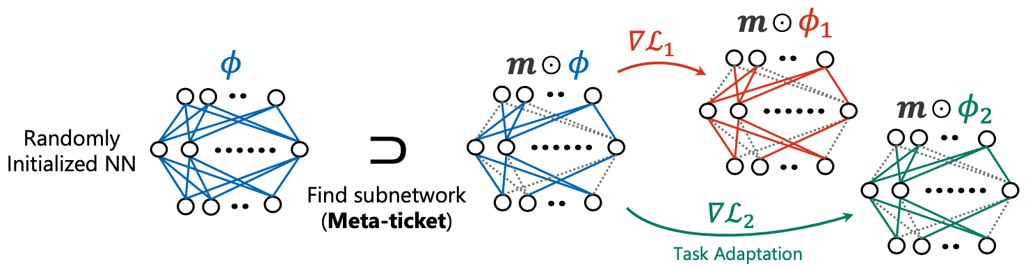
Figure 1: For a randomly initialized neural network $f_{\phi}(x)$, instead of optimizing the initial parameters $\phi$, Meta-ticket finds an optimal subnetwork $f_{\mathbf{m}\odot\phi}(x)$ by meta-optimizing binary parameters $\mathbf{m}$ so that the subnetwork can successfully adapt to tasks with a few samples.

2 Background

2.1 Meta-learning for few-shot learning

Let $X$ be an input space and $Y$ an output space. A distribution $\mathcal{T}$ over $X\times Y$ is called a task. In a standard learning problem, given a task $\mathcal{T}$, we consider a model $f_{\phi}(x):X\to Y$ parameterized by $\phi\in\mathbb{R}^{n}$ and optimize $\phi$ to reduce the expectation value of a loss function $\mathcal{L}:Y\times Y\to\mathbb{R}$. For simplicity, we denote the mean value of the loss function over a dataset $\mathcal{D}\subset X\times Y$ as $\mathcal{L}(f_{\phi};\mathcal{D}):=\frac{1}{|\mathcal{D}|}\sum_{(x,y)\in\mathcal{D}}\mathcal{L}(f_{\phi}(x),y)$.

In meta-learning, we consider a distribution $p(\mathcal{T})$ over the set of tasks $\mathcal{T}$. Meta-learning consists of two optimization stages: adapting to a given task $\mathcal{T}$ (inner optimization) and improving the inner optimization for each task (meta-optimization). To model the inner optimization, we consider a meta-model $F_{\theta}(\mathcal{D})$ parameterized by a meta-parameter $\theta\in\mathbb{R}^{N}$, where $\mathcal{D}$ is a training data sampled i.i.d. from the task $\mathcal{T}$. Given $k\in\mathbb{N}$, we consider the setting of $k$-shot learning where the training data $\mathcal{D}$ consists of $k$ samples, and denote a task with $k$ samples over $(X\times Y)^{k}$ by $\mathcal{T}^{k}$. Then a meta-model for $k$-shot learning is given in the form of $F_{\theta}:(X\times Y)^{k}\to\mathbb{R}^{n}$ with a meta-parameter $\theta\in\mathbb{R}^{N}$. The aim of meta-learning for $k$-shot learning is to optimize the meta-parameter $\theta$ as follows:

$$\min_{\theta\in\mathbb{R}^{N}}\mathbb{E}_{\mathcal{T}\sim p(\mathcal{T})}\mathbb{E}_{\mathcal{D}^{\mathrm{tr}},\mathcal{D}^{\mathrm{val}}\sim\mathcal{T}^{k}}\Big{[}\mathcal{L}\big{(}f_{\phi^{\prime}};\mathcal{D}^{\mathrm{val}}\big{)}\Big{]},\ \ \text{where }\phi^{\prime}=F_{\theta}(\mathcal{D}^{\mathrm{tr}}).$$ (1)

The meta-parameter $\theta$ is optimized to minimize the expected validation loss $\mathcal{L}(f_{\phi^{\prime}};\mathcal{D}^{\mathrm{val}})$ with $\phi^{\prime}$ adapted to a training data $\mathcal{D}^{\mathrm{tr}}$ by the meta-model $F_{\theta}$.

2.2 Model-agnostic meta-learning (MAML)

MAML [13] is a representative method of gradient-based meta-learning [14] which optimizes hyperparameters appearing in gradient descent procedure for $k$-shot learning. Specifically, MAML learns an initial parameter $\phi_{0}\in\mathbb{R}^{n}$ for a model $f_{\phi}(x)$. Here we focus on the case $f_{\phi}(x)$ is an $L$-layered neural network parametrized by $\phi=(\phi^{l})_{l=1\cdots,L}\in\oplus_{l=1,\cdots,L}\mathbb{R}^{n_{l}}$, where $n_{l}$ is the number of parameters in the $l$-th layer. The meta-model of MAML (with $S$ gradient steps) for a neural network $f_{\phi}(x)$ is described as follows:

$$F^{\mathrm{MAML}}_{\phi_{0}}(\mathcal{D}^{\mathrm{tr}}) =\phi_{S-1}$$

$$=\bigg{(}\phi^{l}_{0}-\alpha^{l}\sum_{i=0}^{S-1}\nabla_{\phi^{l}_{i}}\mathcal{L}(f_{\phi_{i}};\mathcal{D}^{\mathrm{tr}})\bigg{)}_{1\leq l\leq L},$$ (2)

where we set $\phi_{i}:=(\phi^{l}_{i})_{1\leq l\leq L}$ as the collection of parameters at $i$-th step, and $\phi^{l}_{i}:=\phi^{l}_{i-1}-\alpha^{l}\nabla_{\phi^{l}_{i-1}}\mathcal{L}(f_{\phi_{i-1}};\mathcal{D}^{\mathrm{tr}})$ as an $i$-th gradient step for $l$-th layer. $\alpha^{l}\in\mathbb{R}_{\geq 0}$ is called an inner learning rate for $l$-th layer, and the gradients $\nabla_{\phi=\phi_{i}}\mathcal{L}(f_{\phi};\mathcal{D}^{\mathrm{tr}})$ in the inner optimization are called task gradients.

2.3 Rapid learning vs. feature reuse

Raghu et al. [50] investigated what makes the MAML algorithm effective in few-shot classification with neural networks. Let $f_{\phi}(x)=h_{\phi_{L}}\circ g_{\Phi}(x)$ be an $L$-layered neural network, where we denote an $(L-1)$-layered neural network $g_{\Phi}(x)$ (feature extractor) and a linear classifier $h_{\phi_{L}}$ (output layer). Under these settings, they considered two phenomenon: rapid learning and feature reuse. Rapid learning means that the neural network $f_{\phi}(x)$ adapt to each task with large changes in the overall parameters $\phi$. Feature reuse means the feature extractor $g_{\Phi}(x)$ meta-learns extracting reusable features for all tasks and is barely changed during the inner optimization. Thus only the output layer $h_{\Phi}(x)$ adapts to each task in the feature reuse case. The question posed by Raghu et al. [50] is as follows: Which of rapid learning and feature reuse is dominant in meta-models trained with MAML?

They empirically showed that the task gradients of the feature extractor in MAML approximately vanish, and thus the feature reuse is dominant in MAML, on few-shot classification benchmarks. Also they introduced a variant of MAML, called ANIL, that lets all parameters of the feature extractor $g_{\Phi}(x)$ be frozen in inner optimization (i.e. setting the inner learning rates $\alpha^{l}=0$ for $1\leq l\leq L-1$). Since ANIL fully satisfies feature reuse by definition, it performs similarly to MAML.

On the other hand, Oh et al. [44] investigated the rapid learning aspects of MAML. They proposed another variant of MAML, called BOIL, that let the parameter of the output layer be frozen in inner optimization (i.e. $\alpha^{L}=0$). In other words, contrary to ANIL, BOIL forces the parameters in the feature extractor to largely change for each task since the parameter of the output layer cannot adapt anymore during inner optimization. Although this formulation seems counterintuitive, they showed that BOIL actually works well. Moreover, BOIL outperforms MAML and ANIL on cross-domain adaptation benchmarks, i.e. evaluating meta-learners with datasets that differ from the one used for meta-learning. The result indicates that the feature reuse in MAML may be suboptimal from the viewpoint of meta-generalization.

3 Methods

In this section, we propose a novel gradient-based meta-learning method called Meta-ticket (Algorithm 1). The aim of Meta-ticket is to meta-learn an optimal sparse NN structure for $k$-shot learning, within a randomly initialized NN. The algorithm can be formulated in parallel to MAML as we will see in Section 3.1. In contrast to MAML, which directly encodes information of a meta-training dataset into the NN parameters, Meta-ticket instead meta-learns which connections between neurons are useful for learning new tasks. Due to this difference in meta-optimization, it is shown that Meta-ticket prefers rapid-learning rather than feature reuse by analyzing task gradients in Section 3.2, which leads to better cross-domain adaptation as demonstrated in Section 4.

3.1 Algorithm: Meta-ticket

Let $f_{\phi}(x)$ be an $L$-layered neural network parametrized by $\phi=(\phi^{l})_{1\leq l\leq L}\in\oplus_{1\leq l\leq L}\mathbb{R}^{n_{l}}=\mathbb{R}^{n}$, where $n_{l}$ is the number of parameters in the $l$-th layer and $n:=\sum_{1\leq l\leq L}n_{l}$. We define a sparse structure for $f_{\phi}(x)$ as a binary mask $\mathbf{m}=(\mathbf{m}^{l})_{1\leq l\leq L}\in\oplus_{1\leq l\leq L}\{0,1\}^{n_{l}}=\{0,1\}^{n}$ whose dimension is same as $\phi$. The corresponding sparse subnetwork is $f_{\mathbf{m}\odot\phi}(x)$ where $\odot$ means an element-wise product in $\mathbb{R}^{n}$. The meta-model $F^{\mathrm{MT}}_{\mathbf{m}}(\mathcal{D}^{\mathrm{tr}})$ for Meta-ticket (with $S$ gradient steps) is described as follows:

$$F^{\mathrm{MT}}_{\mathbf{m}}(\mathcal{D}^{\mathrm{tr}}) =\mathbf{m}\odot\phi_{S-1}$$

$$=\mathbf{m}\odot\bigg{(}\phi^{l}_{0}-\alpha^{l}\sum_{i=0}^{S-1}\nabla_{\phi^{l}_{i}}\mathcal{L}(f_{\mathbf{m}\odot\phi_{i}};\mathcal{D}^{\mathrm{tr}})\bigg{)}_{1\leq l\leq L},$$ (3)

where $\alpha^{l}\in\mathbb{R}$ is an $l$-th inner learning rate, $\phi^{l}_{i}:=\phi^{l}_{i-1}-\alpha^{l}\nabla_{\phi^{l}_{i-1}}\mathcal{L}(f_{\mathbf{m}\odot\phi_{i-1}};\mathcal{D}^{\mathrm{tr}})$ is an $i$-th gradient step, and $\phi_{i}:=(\phi^{l}_{i})_{1\leq l\leq L}$. The differences in Eq. (3.1) from Eq. (2.2) of MAML are the parts involving the mask $\mathbf{m}$. In contrast to MAML optimizing the initial parameter $\phi_{0}$, Meta-ticket optimizes only the binary mask $\mathbf{m}$ and keeps $\phi_{0}$ being a fixed randomly initialized parameter.

The whole algorithm of Meta-ticket is described in Algorithm 1, which involves two functions ${\texttt{CalculateMask}}()$ and ${\texttt{UpdateScore}}()$ to deal with the meta-parameter $\mathbf{m}$. Since $\mathbf{m}$ is a discrete variable, we cannot directly apply the standard NN optimization methods to it. Instead, we optimize a latent continuous parameter $\mathbf{s}=(\mathbf{s}^{l})_{1\leq l\leq L}\in\mathbb{R}^{n}$ corresponding to $\mathbf{m}$, called a score parameter, inspired by Ramanujan et al. [51].

More specifically, we introduce a hyperparameter $p_{\mathrm{init}}\in[0,1]$ called an initial sparsity, which determines the ratio of how many components in $\mathbf{m}$ become zero at the beginning of the algorithm. Also we randomly initialize the score parameter $\mathbf{s}$. Using the initial sparsity $p_{\mathrm{init}}$ and the initialized score $\mathbf{s}$, for each layer $l\in\{1,\cdots,L\}$, we set the layer-wise score threshold $\sigma_{l}\in\mathbb{R}$ as the $\lfloor p_{init}n_{l}\rfloor$-th smallest score $s_{i^{*}}$ in the score parameters $\{s_{i}:1\leq i\leq n_{l}\}$ in the $l$-th layer, before the algorithm starts. During the algorithm, using the fixed thresholds, ${\texttt{CalculateMask}}(\mathbf{s})$ returns the layer-wise masks $(\mathbf{m}^{l})_{1\leq l\leq L}$ where each component $m^{l}_{i}$ of $\mathbf{m}^{l}$ is given by

$$m^{l}_{i}=\begin{cases}0&(s^{l}_{i}\leq\sigma_{l}),\\ 1&(s^{l}_{i}\geq\sigma_{l}).\end{cases}$$ (4)

Although $\mathbf{m}$ is a non-differentiable function in the latent variable $\mathbf{s}$, we can optimize $\mathbf{s}$ by straight-through estimator [7] as previous literature [51]. The optimization step is given by ${\texttt{UpdateScore}}(\mathbf{s},\mathcal{L}_{\mathbf{m}}):=\mathbf{s}-\beta\nabla_{\mathbf{m}}\mathcal{L}_{\mathbf{m}}+(\textrm{momentum})$, i.e. gradient descent with the gradient for $\mathbf{m}$ with respect to the meta-objective $\mathcal{L}_{\mathbf{m}}$ defined by Eq. (1), (3.1), and an outer learning rate $\beta$.

1:$\alpha,\beta\in\mathbb{R}_{\geq 0}$, $p_{\mathrm{init}}\in[0,1]$ $\triangleright$ $\alpha$, $\beta$: inner/outer learning rates, $p_{\mathrm{init}}$: an initial sparsity.

2:$\phi_{0}\in\mathbb{R}^{n}$, $\mathbf{s}\in\mathbb{R}^{n}$$\triangleright$ Randomly initialized parameters.

3:$(\sigma_{l})_{1\leq l\leq L}\in\mathbb{R}^{L}$$\triangleright$ Score thresholds determined by $p_{\mathrm{init}}$ and the initial score $\mathbf{s}$.

4:$\mathbf{m}\leftarrow{\texttt{CalculateMask}}(\mathbf{s})$$\triangleright$ Initialize the binary mask $\mathbf{m}$ using the initial score $\mathbf{s}$

5:while $\mathbf{s}$ is not converged do

6:     Sample $B$ tasks $\mathcal{T}_{1},\cdots,\mathcal{T}_{B}\sim p(\mathcal{T})$

7:     while $b\leftarrow 1,\cdots,B$ do

8:         Sample datasets $\mathcal{D}_{b}^{\mathrm{tr}},\mathcal{D}_{b}^{\mathrm{val}}\sim\mathcal{T}$ for $k$-shot learning of the task $\mathcal{T}_{b}$

9:         $\phi^{\prime}_{b}\leftarrow F^{\mathrm{MT}}_{\mathbf{m}}(\mathcal{D}_{b}^{\mathrm{tr}})$

10:     end while

11:     Calculate the meta-loss $\mathcal{L}_{\mathbf{m}}=\frac{1}{B}\sum_{b=1}^{B}\mathcal{L}\big{(}f_{\phi^{\prime}_{b}}(x);\mathcal{D}_{b}^{\mathrm{val}}\big{)}$

12:      $\mathbf{s}\leftarrow{\texttt{UpdateScore}}(\mathbf{s},\mathcal{L}_{\mathbf{m}})$

13:     $\mathbf{m}\leftarrow{\texttt{CalculateMask}}(\mathbf{s})$

14:end while

15:return $\mathbf{m}$

Algorithm 1  Meta-ticket  (The colored codes are unique to this algorithm.)

3.2 Analysis on task gradients

The meta-models learned with Meta-ticket could have different properties from the ones with MAML since their meta-optimization targets are different. One is a discrete variable $\mathbf{m}$ (Meta-ticket) and another is a continuous variable $\phi_{0}$ (MAML). As discussed in Section 2.3, feature reuse is dominant in the task gradients in MAML, and it may be harmful for meta-generalization capacity. Then a natural question arises: What about the task gradients in Meta-ticket? Here we compare the dynamics of task gradients during meta-training between MAML and Meta-ticket, both empirically and theoretically.

First of all, we performed experiments to see how task gradients of the feature extractor change during meta-training, for different inner learning rate setting (Figure 2). We find that the task gradients in both methods behave similarly in very early phase of meta-training. However, in the rest, the task gradients in Meta-ticket either stop decreasing or even increase, while ones in MAML converge to nearly zero in contrast. These results indicate that Meta-ticket prefers rapid learning rather than feature reuse.

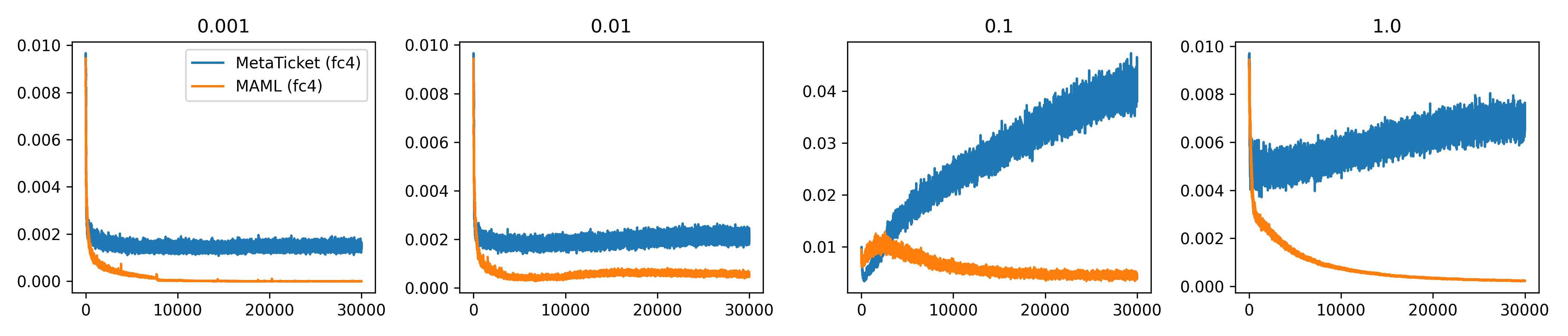
Figure 2: We plotted the mean absolute values of task gradients for the last layer of the feature extractor in a 5-layered MLP (meta-trained on CIFAR-FS as in Section 4.1.3) with varying inner learning rates.

In addition to the above empirical observation, we further investigate why Meta-ticket prefers rapid learning by roughly theoretical argument. For simplicity, we assume that the inner optimization consists of a single gradient step ($S=1$). Now we consider the situation that MAML for $k$-shot learning converges, i.e. the meta-gradients for Eq. (1) with respect to $\phi_{0}$ in Eq. (2.2) approximately vanish as follows:

$$\mathbb{E}_{\mathcal{D}^{\mathrm{tr}},\mathcal{D}^{\mathrm{val}}\sim\mathcal{T}^{k}}\Big{[}\left\lVert\nabla_{\phi_{0}}\mathcal{L}(f_{\phi_{0}-\alpha\nabla\mathcal{L}(f_{\phi};\mathcal{D}^{\mathrm{tr}})};\mathcal{D}^{\mathrm{val}})\right\rVert\Big{]}\leq\varepsilon,$$ (5)

for some $\varepsilon>0$. By Taylor expansion at $\alpha=0$, we have $\nabla_{\phi_{0}}\mathcal{L}(f_{\phi_{0}-\alpha\nabla\mathcal{L}(f_{\phi};\mathcal{D}^{\mathrm{tr}})};\mathcal{D}^{\mathrm{val}})=\nabla_{\phi_{0}}\mathcal{L}(f_{\phi_{0}};\mathcal{D}^{\mathrm{val}})+o(\alpha)$. Now we assume $|\alpha|\ll 1$ and approximate Eq. (5) by

$$\mathbb{E}_{\mathcal{D}^{\mathrm{val}}\sim\mathcal{T}^{k}}\Big{[}\left\lVert\nabla_{\phi_{0}}\mathcal{L}(f_{\phi_{0}};\mathcal{D}^{\mathrm{val}})\right\rVert\Big{]}\leq\varepsilon.$$ (6)

By simply replacing the symbol $\mathcal{D}^{\mathrm{val}}$ in Eq. (6) by $\mathcal{D}^{\mathrm{tr}}$, it follows that

$$\mathbb{E}_{\mathcal{D}^{\mathrm{tr}}\sim\mathcal{T}^{k}}\Big{[}\left\lVert\nabla_{\phi_{0}}\mathcal{L}(f_{\phi_{0}};\mathcal{D}^{\mathrm{tr}})\right\rVert\Big{]}\leq\varepsilon.$$ (7)

The left-hand side of Eq. (7) is nothing but the norm of task gradients in MAML. In other words, when the meta-gradients of MAML converges to zero during meta-training, the task gradients too. On the other hand, if we consider the situation that Meta-ticket converges, we have

$$\mathbb{E}_{\mathcal{D}^{\mathrm{tr}},\mathcal{D}^{\mathrm{val}}\sim\mathcal{T}^{k}}\Big{[}\left\lVert\nabla_{\mathbf{m}}\mathcal{L}(f_{\mathbf{m}\odot(\phi_{0}-\alpha\nabla\mathcal{L}(f_{\mathbf{m}\odot\phi};\mathcal{D}^{\mathrm{tr}}))};\mathcal{D}^{\mathrm{val}})\right\rVert\Big{]}\leq\varepsilon.$$ (8)

By the same argument as Eq. (5–7) and by Leibniz rule, we have

$$\mathbb{E}_{\mathcal{D}^{\mathrm{tr}}\sim\mathcal{T}^{k}}\Big{[}\left\lVert\nabla_{\mathbf{m}}\mathcal{L}(f_{\mathbf{m}\odot\phi_{0}};\mathcal{D}^{\mathrm{tr}})\right\rVert\Big{]}=\mathbb{E}_{\mathcal{D}^{\mathrm{tr}}\sim\mathcal{T}^{k}}\Big{[}\left\lVert\phi_{0}\odot\nabla_{\phi=\mathbf{m}\odot\phi_{0}}\mathcal{L}(f_{\phi};\mathcal{D}^{\mathrm{tr}})\right\rVert\Big{]}\leq\varepsilon.$$ (9)

The last inequality indicates that, if every absolute values of components in $\phi_{0}$ is smaller than $1$ (e.g. when using Kaiming initialization), the norm of the task gradients $\nabla_{\phi}\mathcal{L}(f_{\mathbf{m}\odot\phi};\mathcal{D}^{\mathrm{tr}})$ in Meta-ticket can be larger than $\varepsilon$. This is contrary to the MAML case (Eq. (7)) where the task gradients should be smaller than $\varepsilon$. In conclusion, the empirical observation that Meta-ticket prefers rapid-learning (Figure 2) can be explained by the Taylor expansion analysis under the assumption of the convergence of meta-gradients.

3.3 Some notes on Meta-ticket

Finally, we note some implementation details of Meta-ticket used in our experiments (Section 4).

Parameters that should not be pruned

In typical NN architectures, some kind of parameters should not be pruned by Meta-ticket. One type is non-matrix parameters (e.g. bias terms in linear/convolutional layers, element-wise scaling parameters in Batch/Layer normalization layers and etc). They are often unsuitable for being pruned since pruning them only hurts the adaptation capability of the NN. Another type is the parameters of the output layer for classification tasks. Pruning them means that choosing which neurons in the previous layer can contribute to some $i$-th output of the output layer. However, unlike standard supervised learning setting, $i$-th output can represent an arbitrary class in meta-learning setting. Therefore, pruning the output layer never reflect useful information for the classification tasks and only hurts adaptation capability of the NN. For the parameter $\phi_{i}$ of these types, we initialize and fix the corresponding mask $\mathbf{m}_{i}=1$ (i.e. such $\phi_{i}$ is totally not pruned) throughout the whole Meta-ticket algorithm.

Boosting approximation capacity for small NNs

As known in the studies of strong lottery ticket hypothesis, pruning randomly initialized NNs results in less approximation capacity than standard training by directly optimizing parameters. Similarly, when the size of a given NN is small, Meta-ticket tends to achieve degraded results as we will see in Section 4. For such cases, however, we can adopt the iterative randomization technique (IteRand [9]]) proposed in the lottery ticket literature, which enables us to prune randomly initialized NNs with the same level of approximation capacity as standard training. We will refer the algorithm combining Meta-ticket with the iterative randomization as Meta-ticket+IteRand in our experiments (Section 4.1.1).

4 Experiments

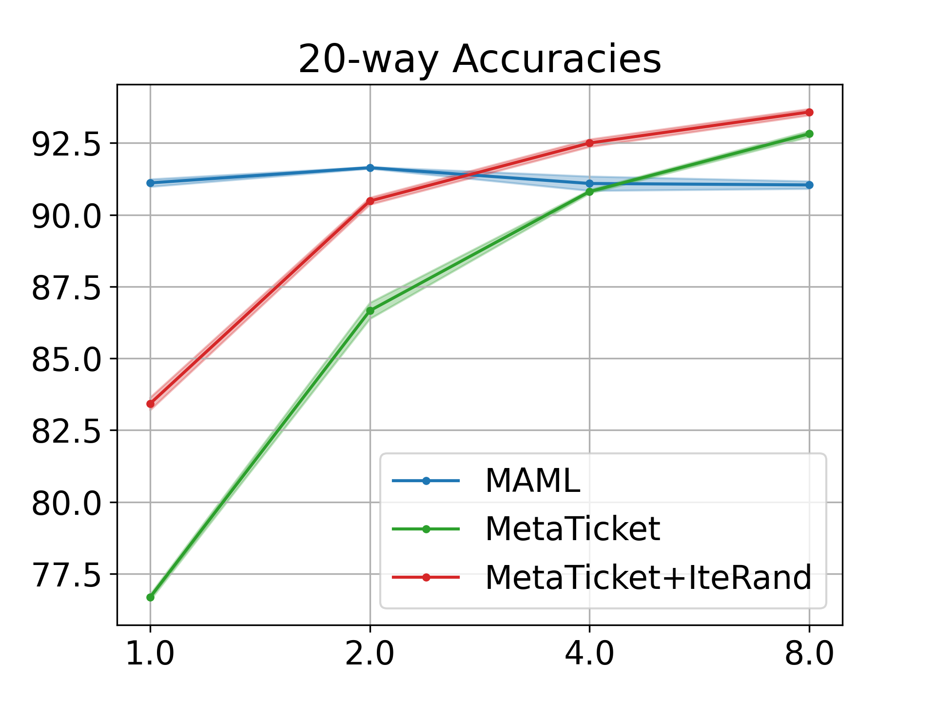
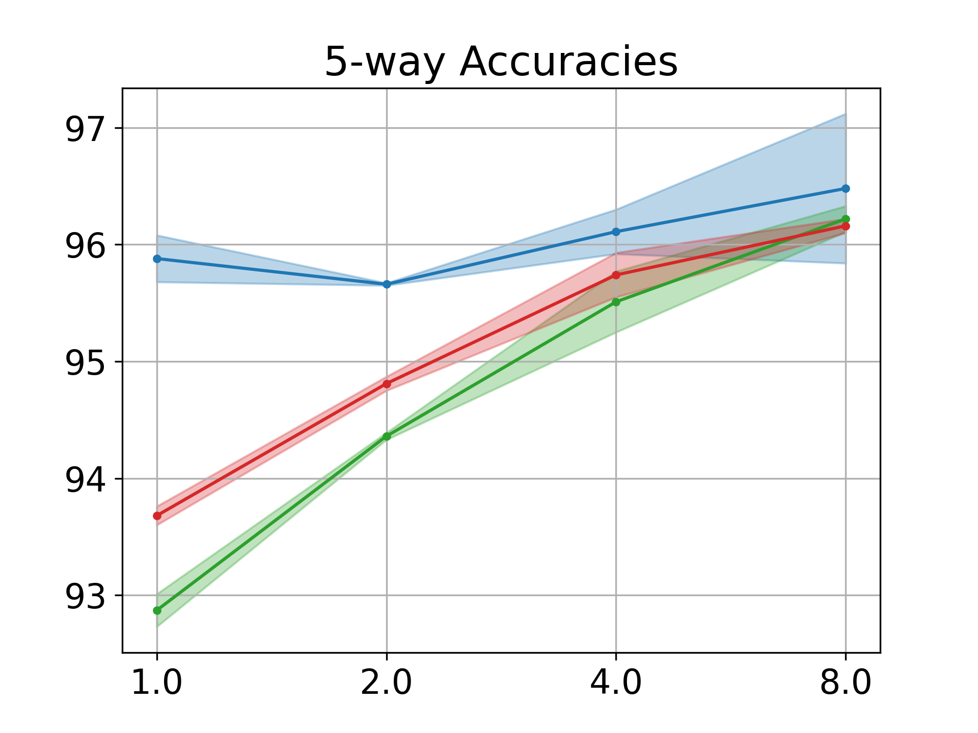
Figure 3: 5-shot accuracies on Omniglot with MLPs of various sizes. The x-axis is width factor.

In this section, we conduct experiments to evaluate meta-generalization performance of Meta-ticket on multiple benchmarks of few-shot image classification. As baseline methods, we choose MAML [13] and its variants (ANIL [50] and BOIL [44]) since Meta-ticket is formulated in a parallel way to MAML and can be considered as another approach of gradient-based meta-learning. The details on every datasets, NN architectures and hyperparameters in our experiments are given in Appendix A.

4.1 Experiments with MLPs

In this subsection, we investigate the properties of Meta-ticket using $5$-layered multilayer perceptrons (MLPs) with the ReLU activation function and batch normalization layers [24]. Since MLPs are fully-connected neural networks (NNs) designed for general tasks, we can see how Meta-ticket performs on NNs involving little inductive biases of task information. In other words, Meta-ticket is expected to learn inductive biases from a given meta-training dataset and encode them as sparse structures in fully-connected layers of the MLPs.

We use the following small-scale datasets for meta-learning with MLPs: Omniglot [29, 59], CIFAR-FS [8], VGG-Flower [43, 30] and Aircraft [37, 30]. Omniglot is a relatively easy dataset of image classification tasks, which consists of monochrome $28\times 28$ images of handwritten characters from different alphabets in the world. CIFAR-FS, VGG-Flower and Aircraft are also datasets of classification tasks, with more natural and colorful $32\times 32$ images.

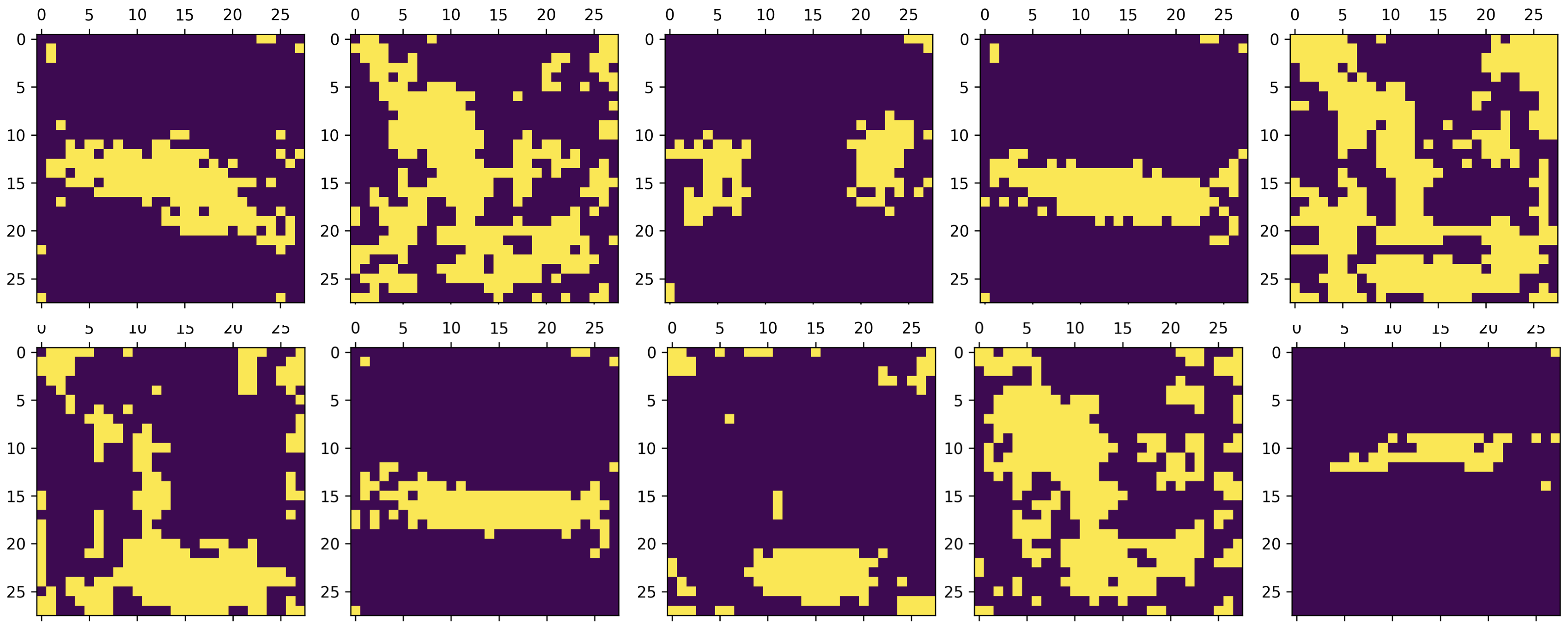
Figure 4: We visualize $28\times 28$ binary masks $\mathbf{m}$ for the first fully-connected layer in 5-MLP with the same constant parameters. The light (resp. dark) color represents $\mathbf{m}_{ij}=1$ (resp. $\mathbf{m}_{ij}=0$).

Table 1: Cross-domain evaluation for 5-shot 5-way classification with 5-MLP.

Meta-train	CIFAR-FS			VGG-Flower
Meta-test	CIFAR-FS	VGG-Flower	Aircraft	CIFAR-FS	VGG-Flower	Aircraft
MAML [13]	$53.48\pm 0.36\%$	$58.60\pm 0.59\%$	$28.95\pm 0.76\%$	$36.67\pm 0.86\%$	$59.16\pm 0.69\%$	$28.50\pm 0.75\%$
ANIL [50]	$50.37\pm 0.68\%$	$53.32\pm 0.62\%$	$26.86\pm 0.77\%$	$34.94\pm 1.14\%$	$58.87\pm 1.30\%$	$27.07\pm 0.73\%$
BOIL [44]	$55.47\pm 1.13\%$	$62.46\pm 0.15\%$	$\mathbf{33.36}\pm 0.84\%$	$36.49\pm 0.98\%$	$58.15\pm 0.86\%$	$28.74\pm 0.97\%$
Meta-ticket	$\mathbf{55.51}\pm 0.47\%$	$62.34\pm 0.17\%$	$31.85\pm 0.31\%$	$\mathbf{40.82}\pm 0.43\%$	$\mathbf{64.09}\pm 0.28\%$	$\mathbf{30.60}\pm 0.63\%$
+ BOIL	$\mathbf{56.06}\pm 0.57\%$	$\mathbf{63.31}\pm 0.07\%$	$33.02\pm 0.32\%$	$\mathbf{42.56}\pm 0.41\%$	$\mathbf{65.69}\pm 0.20\%$	$\mathbf{33.86}\pm 0.36\%$

4.1.1 Experiments with various network sizes

As known in the literature [51, 49] of strong lottery tickets, in general, the pruning-only optimization like Meta-ticket tends to suffer from the lacked model capacity especially when using small NNs. To check how Meta-ticket suffers from the lacked capacity, we evaluate Meta-ticket with MLPs of various network widths, comparing to MAML as a reference. In Figure 3, we plot $5$-shot meta-test accuracies on Omniglot. As we guessed in the above, Meta-ticket suffers from the degraded performance with small network widths. On the other hand, we can see that Meta-ticket even achieves superior accuracies when using larger networks on more difficult tasks of $20$-way classification. Also, as we noted in Section 3.3, the results with small NNs is largely improved by applying the iterative randomization [9] (Meta-ticket+IteRand) from the lottery ticket literature.

4.1.2 The effect of sparse structures themselves

While Meta-ticket never directly meta-optimize the randomly initialized parameters in NNs, it can be considered that the parameter selection by Meta-ticket may produce a similar effect to the parameter optimization like MAML. Now the following question arises: Can sparse NN structures solely be effective for few-shot learning without any information on initial parameters? To answer this question, we consider an extremely restricted setting that all parameters are initialized with the same constant value, which prevents parameters from carrying any information about tasks. We conducted experiments in this setting on Omniglot $5$-shot $5$-way classification with $3$ adaptation steps. The results are as follows: The subnetworks obtained by Meta-ticket achieve $71.59\pm 1.51~{}\%$ in meta-test accuracy while random subnetworks achieve only about $33~{}\%$. This shows that Meta-ticket can find subnetworks being effective for few-shot learning even without leveraging any parameter signals. Also we visualize the sparse structures obtained by Meta-ticket in Figure 4. It indicates that the above success is due to finding sparse structures that can exploit the locality of the images in Omniglot.

4.1.3 Evaluation on different domain datasets

Finally, we evaluate the cross-domain adaptation ability of Meta-ticket with a $5$-layered MLP (denoted by 5-MLP). As discussed in Section 2.3 based on the previous works [50, 44], MAML tends to suffer when adapting to tasks in unknown domains due to its feature reuse property. In contrast, since Meta-ticket prefers rapid learning rather than feature reuse (see Section 3.2), it is expected that the subnetworks obtained by Meta-ticket can generalize to tasks in unknown domains.

We conduct the cross-domain evaluation on CIFAR-FS, VGG-Flower and Aircraft. CIFAR-FS consists of classification tasks with relatively general classes from CIFAR-100 [28], and VGG-Flower and Aircraft have specialized classes. Table 1 shows the results. Meta-ticket outperforms MAML by a larger margin especially for tasks in unknown domains (i.e. different from the meta-training dataset), which indicates that Meta-ticket successfully discovered domain-generalizable sparse structures. Also, we compare with ANIL [50] and BOIL [44] as baselines, which are variants of MAML with modified inner learning rates (see Section 2.3 for details). In particular, BOIL satisfies the rapid learning property by definition and thus better meta-generalization than MAML and ANIL. In parallel to MAML, we can consider the variant of Meta-ticket with $\alpha_{L}=0$ (i.e. the same modification as BOIL) which is denoted by Meta-ticket+BOIL. Since Meta-ticket+BOIL achieves almost the same or better accuracies than BOIL, we find out that the Meta-ticket-based method also benefits from the modification and still achieves superior meta-generalization than the MAML-based methods.

4.2 Experiments with CNNs on mini-Imagenet

Table 2: Cross-domain evaluation for 5-shot 5-way classification with large CNNs, which are meta-trained on miniImageNet and meta-tested on miniImageNet, CUB and Cars.

Networks	ResNet-12			WideResNet-28-10
Meta-train	miniImageNet			miniImageNet
Meta-test	miniImageNet	CUB	Cars	miniImageNet	CUB	Cars
MAML	$67.47\pm 1.31\%$	$54.44\pm 0.23\%$	$43.68\pm 1.44\%$	$62.83\pm 2.47\%$	$46.46\pm 3.54\%$	$37.09\pm 2.49\%$
ANIL	$66.88\pm 1.59\%$	$53.90\pm 1.17\%$	$40.87\pm 3.95\%$	$63.01\pm 0.82\%$	$46.65\pm 0.20\%$	$37.51\pm 1.95\%$
BOIL	$69.67\pm 0.66\%$	$58.79\pm 1.48\%$	$47.11\pm 1.10\%$	$65.82\pm 5.26\%$	$55.92\pm 0.78\%$	$42.08\pm 0.50\%$
Meta-ticket	$\mathbf{71.31}\pm 0.29\%$	$57.97\pm 0.53\%$	$45.90\pm 0.50\%$	$\mathbf{74.63}\pm 0.22\%$	$\mathbf{63.26}\pm 0.86\%$	$\mathbf{52.54}\pm 0.70\%$
+ BOIL	$\mathbf{74.23}\pm 0.30\%$	$\mathbf{64.06}\pm 1.05\%$	$\mathbf{55.20}\pm 0.64\%$	$\mathbf{73.55}\pm 0.17\%$	$\mathbf{62.19}\pm 0.69\%$	$\mathbf{51.41}\pm 0.83\%$

Meta-ticket also can be applied to convolutional neural networks (CNNs). Although CNNs already have sparse NN structures as convolutional kernels, they can still benefit from the rapid learnable nature of Meta-ticket. To evaluate the practical benefits as well as meta-generalization ability, we conducted cross-domain evaluation on near real-world datasets. We employed miniImagenet dataset [59, 52], which consists of image classification tasks with $84\times 84$ images and general classes, for meta-training/testing and specialized datasets such as classification of birds (CUB dataset [63, 21]) and cars (Cars dataset [27, 57]) for meta-testing. For CNN architectures, we chose near-practical deep ones: ResNet-12 [20] and WideResNet-28-10 [66].

The results are shown in Table 2. Meta-ticket and its BOIL-variant consistently outperform MAML-based methods, by a large margin especially when evaluated on specialized domains, probably because Meta-ticket can adjust its feature extractor to recognize fine-grained differences by the rapid learning. Moreover, while MAML struggles to exploit the potential of a larger network such as WideResNet-28-10, Meta-ticket can benefit from such scaling up of network size.

5 Related Work

Gradient-based meta-learning

Meta-learning [6, 54, 55] has been studied for decades to equip computers with learning capabilities. There are several approaches depending on how the inner optimization is modeled. Black-box meta-learning approaches model the inner optimization by recurrent [22, 3, 52] or feedforward [41, 19] neural networks. Gradient-based meta-learning [14] models the inner optimization by one or multiple steps of gradient descent, which leads to sample-efficient meta-learning due to the strong inductive bias on the inner optimization. MAML [13] is a representative method of the gradient-based approach, which meta-learns initial parameters for the inner optimization. There are also extensions of MAML, including meta-learnable learning rates [34] and transformation matrices [47, 15, 5, 60] of the inner optimization. Some works [50, 44] discussed on feature reuse of MAML, and pointed out that it may hurt the meta-generalization capacity of MAML. Since our proposed method (Meta-ticket) is another gradient-based meta-learning method formulated in parallel to MAML, most of extensions of MAML can also be applied to Meta-ticket. Finally, we note on related works involving both meta-learning and pruning. Tian et al. [56] and Gao et al. [18] investigated magnitude-based pruning methods for meta-learning of MAML, while our work focused on meta-learning by pruning only. Alizadeh et al. [2] exploits meta-gradient to prune randomly initialized neural networks. Although the methodology is very similar to ours, their target is pruning at initialization [33] for standard learning, not few-shot learning.

Learning neural network structures from data

Some prior works [17, 42, 68] attempt to automatically learn inductive biases on neural network structures conventionally designed by human. Neyshabur [42] pointed out that the superior generalization capacity of CNNs is mainly due to sparse structures, which enables to leverage locality of image data. Also they proposed a pruning scheme to automatically find such sparse structures, but it does not involve meta-learning and not designed for few-shot learning. Another line of research is neural architecture search (NAS [70]). In particular, meta-learning-based NAS [36, 31, 65] can efficiently search neural architectures. Also, NAS for few-shot learning [25, 35, 12, 62, 61] is closely related to our work. Since NAS aims to automatically design how to connect pre-defined blocks and not to find sparse structures in each block, it is orthogonal to our approach of finding sparse NN structures.

Lottery ticket hypothesis

Lottery ticket hypothesis (LTH) is originally proposed in Franckle and Carbin [16], which claims the existence of sparse subnetworks in randomly initialized NNs such that the former can achieve as good accuracy as the latter after training. Inspired by the analysis in Zhou et al. [69], Ramanujan et al. [51] proposed to train NNs by pruning randomly initialized NNs (weight-pruning optimization) without any optimization of the initial parameters (weight optimization). Their hypothesis are formulated as strong LTH: There exist sparse subnetworks in randomly initialized NNs that already achieves good accuracy without training. The follow-up works [38, 45, 49] theoretically proved it under assumption on the network size. From the viewpoint of LTH, Meta-ticket can be considered as a meta-learning method with weight-pruning optimization, and MAML as one with weight optimization. Surprisingly, even though weight-pruning optimization tends to achieve worse accuracies than weight optimization in general, Meta-ticket outperforms MAML by a large margin in cross-domain evaluation.

Applications of sparse NN structures to continual learning

Continual learning [55, 46] aims to learn new tasks sequentially without forgetting the capacity learned from past tasks. To handle such multiple tasks, some works [40, 39, 23, 64] leverage sparse NN structures in continual learning. In particular, the approach by Wortsman et al. [64] shares a similar spirit to ours in that they leverage subnetworks of a randomly initialized neural network. Unlike our approach, which finds an optimal subnetwork common to multiple tasks, they leverage task-specific subnetworks to separate learned results from multiple tasks.

6 Limitations

As suggested from the theory of strong lottery tickets [38, 45, 49], Meta-ticket also tends to degrade with small NNs compared to MAML (see Section 4.1.1). However, the degradation can be reduced largely by iterative randomization technique [9] as explained in Section 3.3. Moreover, Meta-ticket actually outperforms MAML when using larger NNs. We regard Meta-ticket as an alternative gradient-based meta-learning of MAML, and thus one can switch either of them to use depending on the NN scale. Also, since our theoretical analysis on task gradients (Section 3.2) heavily depends on Taylor series approximation, it holds only when the inner learning rates are sufficiently small. For general cases, it might require the arguments involving the theory on gradient-based meta-learning with SGD. Hence, proving the feature reuse in MAML still remains an open problem.

7 Conclusion

In this work, we investigated sparse NN structures that are effective for few-shot learning. We proposed a novel gradient-based meta-learning method called Meta-ticket, which discovers optimal subnetworks for few-shot learning within randomly initialized neural networks. While Meta-ticket is formulated in parallel to MAML, we found that Meta-ticket prefers rapid learning rather than feature reuse in contrast to MAML. As a result, since the resulting feature extractor obtained by Meta-ticket can recognize specialized features for each task, Meta-ticket can achieve superior meta-generalization especially on unknown domains. Moreover, we found that Meta-ticket can benefit from scaling up of the size of neural networks while MAML struggles to exploit the potential of large NNs. We hope that this work opens up a new research direction in gradient-based meta-learning, focusing on sparse NN structures rather than initial parameters.

Appendix A Details on experiments

A.1 Datasets

In our experiments in Section 4, we used the following datasets for meta-training/validation/testing. We used the Torchmeta library [10] for the implementations.

• Omniglot  Omniglot [29] is a dataset of monochrome $28\times 28$ images of $1623$ handwritten characters from $50$ different alphabets, which is distributed under the MIT License. For meta-learning, the mutually disjoint $1028$/$172$/$423$ characters are used for meta-traininig/validation/testing respectively, following Vinyals et al. [59], where each character is randomly rotated by $0,90,180,270$ degrees.

• CIFAR-FS  CIFAR-FS is a dataset for meta-learning introduced in Bertinetto et al. [8], which consists of $32\times 32$ images with $100$ classes from the CIFAR-100 dataset[28]. The mutually disjoint $64$/$16$/$20$ classes [10] are used for meta-training/validation/testing respectively.

• VGG-Flower  VGG-Flower^{* ‣ • ‣ A.1}[43] is a dataset of images of $102$ species of flowers. For meta-learning, the mutually disjoint $71$/$16$/$15$ classes [30] are used for meta-training/validation/testing respectively.

• Aircraft  Aircraft [37] is a dataset of images of $102$ classes of aircrafts, which is provided exclusively for non-commercial research purposes. For meta-learning, the mutually disjoint $70$/$15$/$15$ classes [30] are used for meta-training/validation/testing respectively.

• miniImageNet  MiniImageNet is a dataset for meta-learning introduced in Vinyals et al [59], which consists of $84\times 84$ images of $100$ classes collected from the ImageNet dataset[53]. The mutually disjoint $64$/$16$/$20$ classes [52, 10] are used for meta-training/validation/testing respectively.

• CUB  CUB^{* ‣ • ‣ A.1} [63] is a dataset of images of $200$ species of birds. For meta-learning, the mutually disjoint $100$/$50$/$50$ classes [10] are used for meta-training/validation/testing respectively.

• Cars  Cars [27] is a dataset of images of $196$ classes of cars, which is provided for research purposes. For meta-learning, the mutually disjoint $98$/$49$/$49$ classes [57] are used for meta-training/validation/testing respectively.

A.2 Network architectures

A.2.1 5-layered MLPs (for Omniglot in Section 4.1.1)

In Table 3, we summarize the network architecture of 5-layered MLPs used in Section 4.1.1. To analyze the effect of the network size, we introduced the width factor $\rho\in\mathbb{N}$ by which the dimensions of the intermediate outputs are multiplied.

Table 3: The architecture of 5-layered MLPs for Omniglot ($\rho$: a width factor).

Layers	Output dimensions
Flatten	$784\ (=28\times 28)$
Linear $\to$ BatchNorm $\to$ ReLU	$256\rho$
Linear $\to$ BatchNorm $\to$ ReLU	$128\rho$
Linear $\to$ BatchNorm $\to$ ReLU	$64\rho$
Linear $\to$ BatchNorm $\to$ ReLU	$64\rho$
Linear	$\#\text{ ways }(5\text{ or }20)$

A.2.2 5-MLP (for CIFAR-FS, VGG-Flower and Aircraft in Section 4.1.3)

In Table 4, we summarize the network architecture of 5-MLP used in Section 4.1.3. For a fair comparison, the hidden dimensions are chosen so that the baseline method (MAML) achieves a good performance.

Table 4: The architecture of 5-MLP for CIFAR-FS.

Layers	Output dimensions
Flatten	$3072\ (=3\times 32\times 32)$
Linear $\to$ BatchNorm $\to$ ReLU	$1024$
Linear $\to$ BatchNorm $\to$ ReLU	$512$
Linear $\to$ BatchNorm $\to$ ReLU	$256$
Linear $\to$ BatchNorm $\to$ ReLU	$128$
Linear	$5$

A.2.3 CNNs (for miniImageNet, CUB and Cars in Section 4.2)

For ResNet12, we employed the architecture used in Lee et al. [32], following the setting of the BOIL paper by Oh et al. [44]. For WideResNet-28-10, we used the architecture provided in the learn2learn library [4], which is the setting used in Dhillon et al. [11]. The number of parameters for these architectures is summarized in Table 5.

Table 5: The numbers of parameters for CNNs in our experiments.

Networks	# of parameters
ResNet-12	8.0 M
WideResNet-28-10	36.5 M

A.3 Hyperparameters

In our experiments, there are two types of hyperparameters: (1) ones common to gradient-based meta-learning, including MAML and Meta-ticket, and (2) ones specific to Meta-ticket.

A.3.1 Common hyperparameters

Here we summarize hyperparameters common to gradient-based meta-learning: the number of iterations of meta-learning, the number of inner gradient steps $S$, batch size $B$ for meta-learning, outer learning rate (LR), inner LR, and optimizers. In our experiments, we trained all meta-models (MAML, ANIL, BOIL and Meta-ticket) for $30000$ iterations with $S=1$ and $B=4$. Other hyperparameters are summarized in Table 6. For MAML-based methods, we followed the settings in the previous work [44].

Table 6: Hyperparameters common to gradient-based meta-learning methods.

Meta-training datasets	Methods	Outer LR	Inner LR	Optimizer
Omniglot	MAML	0.001	0.4	Adam [26]
	Meta-ticket	10.0	0.4	SGD
CIFAR-FS, VGG-Flower	MAML	0.001	0.5	Adam
	Meta-ticket	10.0	0.5	SGD
miniImageNet	MAML	0.0006	0.3	Adam
	Meta-ticket	10.0	0.3	SGD

A.3.2 Specific hyperparameters to Meta-ticket

• Initial sparsity For the initial sparsity $p_{\mathrm{init}}\in[0,1]$, we chose $p_{\mathrm{init}}=0.0$ (i.e. the initial subnetwork is equal to the entire network) since we found that a lower initial sparsity tends to be better in terms of meta-generalization ability. However, as we can see in Section B.2, we can get a more sparse subnetwork if we use a larger initial sparsity.

• Parameter initialization In Meta-ticket, there are two initialization for the score parameter $\mathbf{s}$ and the network parameter $\phi_{0}$. (See Section 3.1 for the notation.) We employed Kaiminig uniform initialization [1] for $\mathbf{s}$, and Kaiming normal initialization [1] for $\phi_{0}$.

• Optimizer As a (meta-)optimizer for the score parameters of Meta-ticket, following the strong lottery ticket literature [51, 9], we employed stochastic gradient descent (SGD) with a cosine scheduler. Also, we found that the outer learning rate needs to be larger than the standard ones, and thus we set the learning rate as $10.0$. (See also Section B.1.)

• Iterative randomization Iterative randomization (IteRand, proposed by Chijiwa et al. [9]) is a technique to boost the performance of weight-pruning optimization, especially for small neural networks, by re-initializing the pruned parameters every $K$ iterations. We chose the re-initialization frequency as $K=1000$.

A.4 Implementations and training details

Implementations

We implemented Meta-ticket and all experiments by using the PyTorch [48], learn2learn [4] and Torchmeta [10] libraries. Also, the implementation of ResNet-12 is based on the one implemented by Oh et al. [44].

Computational resources

In meta-training and meta-testing, we used a single NVIDIA V100 GPU or NVIDIA A100 GPU for each experiment. For all of our experimental results, we reported means and one standard deviations for three random seeds.

Computational overhead of Meta-ticket

Even though Meta-ticket has additional parameters for scores compared to MAML, there was little difference in meta-training time. For example, in the meta-training on miniImageNet with ResNet12 (Section 4.2), Meta-ticket takes about 583 seconds for 1000 iterations on an A100 GPU machine, while MAML takes about 560 seconds. Hence the computational overhead in this case is only about $4\%$.

Appendix B Additional experiments

B.1 Learning rates for Meta-ticket

We searched the outer learning rate for the score parameter of Meta-ticket, using the 1-shot 5-way benchmark on miniImageNet with ResNet-12. Table 7 shows the meta-validation accuracies for various learning rates. In contrast to standard training, relatively large learning rates are suitable for the score parameter $\mathbf{s}=(s_{i})_{1\leq i\leq N}$. This is because the actual value of each $s_{i}$ is not important and just whether or not $s_{i}$ is above the threshold $\sigma$ matters.

Table 7: Meta-validation accuracies for various learning rates on the 1-shot 5-way miniImageNet benchmark with ResNet-12.

Learning rate	0.01	0.1	1.0	10.0	100.0
Accuracy	$34.87\pm 1.40\%$	$42.97\pm 0.67\%$	$53.67\pm 2.12\%$	$\mathbf{54.30}\pm 2.52\%$	$51.97\pm 0.64\%$

B.2 Effects of the initial sparsity

In this section, we analyze the effects of the initial sparsity $p_{\mathrm{init}}$ to the resulting subnetworks. Figure 5 shows the sparsity of the subnetwork in ResNet-12 obtained by Meta-ticket during the meta-training phase. Although the final sparsity largely depends on the initial sparsity, the sparsity changes in the direction of the half sparsity, consistently in every case. On the other hand, from the viewpoint of meta-generalization, we can see that the meta-validation accuracy tends to be better if we start from a lower initial sparsity (Table 8). Also, in Figure 6, we plotted the meta-validation accuracy curves during meta-training for each initial sparsity.

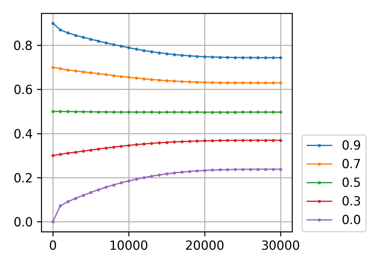
Figure 5: For each initial sparsity ($p_{\mathrm{init}}=0.0,0.3,0.5,0.7,0.9$), we plotted the sparsity of the subnetwork in ResNet-12 obtained by Meta-ticket during the meta-training phase. The x-axis is the number of meta-training iterations.

Table 8: Meta-validation accuracies for various initial sparsities in 1-shot 5-way setting.

Initial sparsity	0.0	0.3	0.5	0.7	0.9
Accuracy	$\mathbf{54.70}\pm 1.90\%$	$53.40\pm 0.50\%$	$52.27\pm 0.84\%$	$51.57\pm 0.64\%$	$51.53\pm 0.92\%$

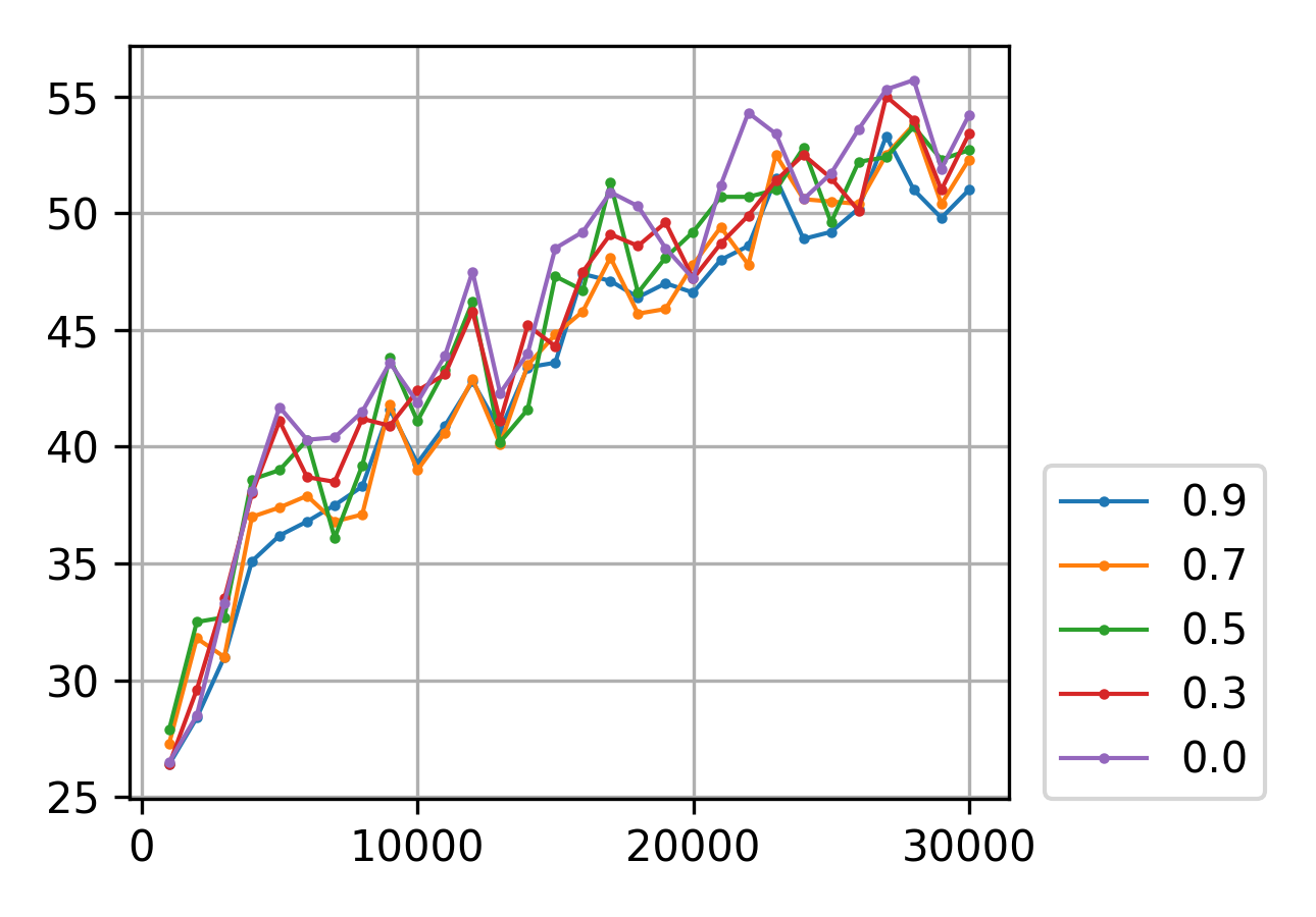
Figure 6: For each initial sparsity ($p_{\mathrm{init}}=0.0,0.3,0.5,0.7,0.9$), we plotted meta-validation accuracies during meta-training. The x-axis is the number of meta-training iterations.

B.3 Cross-domain evaluation in 1-shot 5-way setting

Table 9 shows the results of cross-domain evaluation on miniImageNet with the setting of 1-shot learning. We meta-trained ResNet-12 and WideResNet-28-10 by Meta-ticket and MAML, with the 1-shot learning tasks from the miniImageNet dataset. There seems to be little difference between the results of MAML and Meta-ticket (except for the case of WideResNet-28-10 evaluated on miniImageNet itself), in contrast to the 5-shot setting (Section 4.2). The results may be due to the lack of training samples during the inner optimization in the 1-shot setting, where we cannot take enough advantage of the rapid learning nature of Meta-ticket.

Table 9: Cross-domain 1-shot 5-way evaluation with ResNet-12 and WideResNet-28-10

Networks	ResNet-12			WideResNet-28-10
Meta-train	miniImageNet			miniImageNet
Meta-test	miniImageNet	CUB	Cars	miniImageNet	CUB	Cars
MAML	$56.25\pm 1.28\%$	$45.85\pm 0.77\%$	$35.85\pm 1.18\%$	$50.59\pm 0.54\%$	$42.12\pm 0.57\%$	$33.50\pm 0.88\%$
Meta-ticket	$56.17\pm 0.91\%$	$45.95\pm 0.81\%$	$35.99\pm 2.00\%$	$54.12\pm 1.24\%$	$41.77\pm 0.92\%$	$34.26\pm 0.31\%$

B.4 Comparison with state-of-the-art methods

In Table 10, we compare our cross-domain evaluation results (given in Table 2 in Section 4.2) to state-of-the-art methods (MetaOptNet [32] and Feature-wise Transformation [57]) other than MAML-based methods. Both of these state-of-the-art methods achieve higher meta-test accuracy on miniImageNet, which is the dataset used in meta-training, than variants of MAML and Meta-ticket. This would be because these methods can leverage their strong feature extractor on the meta-training dataset. However, these two state-of-the-art methods are largely degraded when meta-tested on CUB and Stanford Cars. On the other hand, Meta-ticket + BOIL achieves similar accuracy as the feature-wise transformation method on CUB, and the highest accuracy on Stanford Cars in the table. This would show the strength of the rapid learning nature of Meta-ticket.

Table 10: Comparison with state-of-the-art methods in 5-shot 5-way cross-domain classification.

Meta-training dataset	miniImageNet
Meta-test dataset	miniImageNet	CUB	Cars
MAML	$67.47\pm 1.31\%$	$54.44\pm 0.23\%$	$43.68\pm 1.44\%$
ANIL	$66.88\pm 1.59\%$	$53.90\pm 1.17\%$	$40.87\pm 3.95\%$
BOIL	$69.67\pm 0.66\%$	$58.79\pm 1.48\%$	$47.11\pm 1.10\%$
Meta-ticket (Ours)	$71.31\pm 0.29\%$	$57.97\pm 0.53\%$	$45.90\pm 0.50\%$
+ BOIL (Ours)	$74.23\pm 0.30\%$	$64.06\pm 1.05\%$	$\mathbf{55.20\pm 0.64}\%$
MetaOptNet-SVM-trainval [32]	$80.00\pm 0.45\%$	$54.67\pm 0.56\%$‡ ‣ 10	$45.90\pm 0.49\%$‡ ‣ 10
GNN + Feature-wise Transformation [57]	$\mathbf{81.98\pm 0.55}\%$‡ ‣ 10	$\mathbf{66.98\pm 0.68}\%$‡ ‣ 10	$44.90\pm 0.64\%$‡ ‣ 10

B.5 Results on specific to general/specific adaptation

In Section 4.2, we evaluated the cross-domain adaptation from a general-domain dataset (miniImageNet) to specific-domain datasets (CUB and Cars). Here we present additional experimental results (Table 11) of cross-domain adaptation from a specific-domain dataset (CUB) to the other datasets. Although there are only small difference between MAML-based methods and Meta-ticket when evaluated on the meta-training dataset itself, Meta-ticket has a larger gain on the specific to general/specific cross-domin adaptation. The results indicate that, while MAML-based methods successfully encode useful features into their initial parameters to classify the fine-grained classes of bird species (in CUB), the encoded features are not enough useful for classifying other categories in miniImageNet and Cars datasets.

Table 11: Results on specific to general/specific adaptation.

Meta-training dataset	CUB
Meta-test dataset	CUB	miniImageNet	Cars
MAML	$78.92\pm 0.62\%$	$43.03\pm 0.26\%$	$38.95\pm 0.42\%$
BOIL	$\mathbf{83.70\pm 0.40}\%$	$49.17\pm 1.30\%$	$43.93\pm 1.39\%$
Meta-ticket	$80.49\pm 0.50\%$	$46.01\pm 0.55\%$	$40.24\pm 0.92\%$
+ BOIL	$83.28\pm 0.44\%$	$\mathbf{53.82\pm 0.92}\%$	$\mathbf{48.85\pm 0.56}\%$

B.6 Detailed plots of inner gradients during meta-training

In Section 3.2, we presented the plots of inner gradient norms of the last layer of the feature extractor of 5-MLP during meta-training on CIFAR-FS. Here we provide more detailed plots for every feature extracting layer of 5-MLP on CIFAR-FS (Figure 7) and VGG-Flower (Figure 8) with log-scaled y-axis. In both cases, the inner gradient norms in MAML tend to converge to nearly zero, while the ones in Meta-ticket stop to decrease or even start to increase at some iteration. However, there are some exceptions particularly when inner learning rate is relatively large. This indicates that our theoretical discussion for a small inner learning rate (given in Section 3.2) does not necessarily describe the dynamics of inner gradients for large inner learning rates.

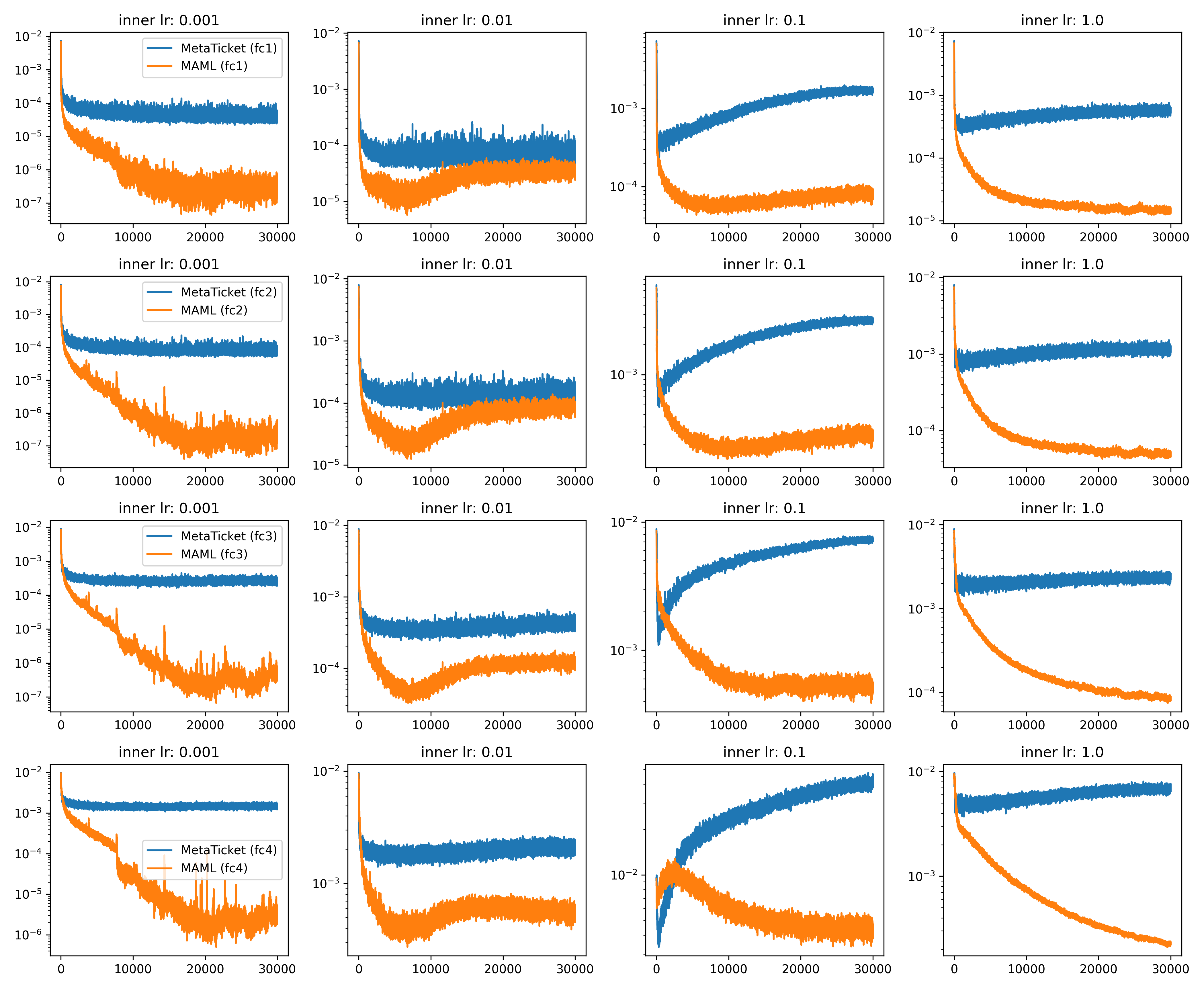
Figure 7: Inner gradient norms (log scale) of 5-MLP meta-trained on CIFAR-FS with various inner learning rates $\alpha\in\{0.001,0.01,0.1,1.0\}$ for each fully-connected layer of the feature extractor.

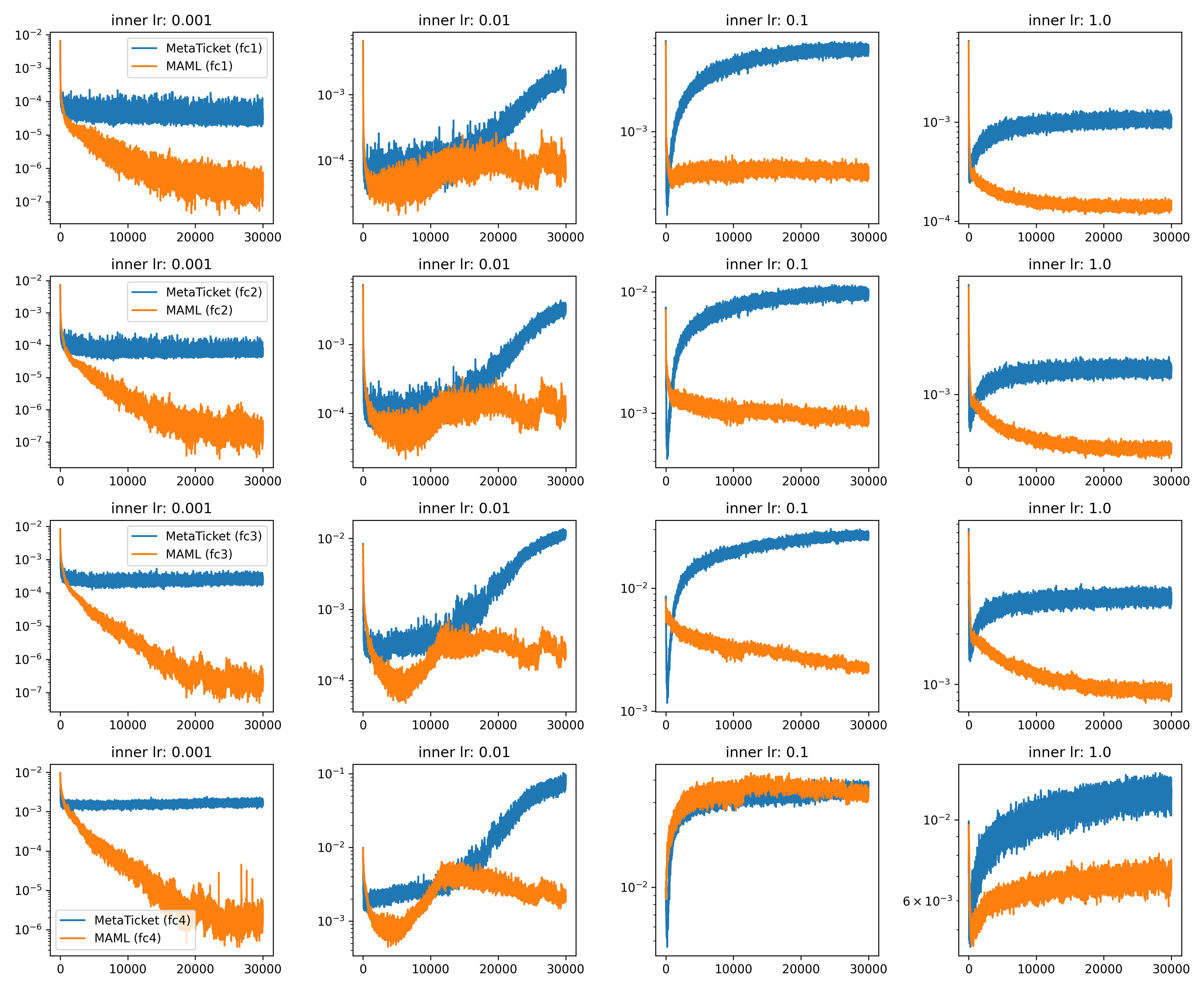
Figure 8: Inner gradient norms (log scale) of 5-MLP meta-trained on VGG-Flower with various inner learning rates $\alpha\in\{0.001,0.01,0.1,1.0\}$ for each fully-connected layer of the feature extractor.

Appendix C Experiments on a regression benchmark

In this section, we report the results on a toy regression benchmark of learning to predict a given sine function, which is called Sinusoid regression [13], in the setting of 5-shot learning with 5 gradient steps. We used a simple 3-layered ReLU multilayered perceptron (MLP) with $1$-dimensional input/output and $40$-dimensional hidden layers, following the setting in Finn et al. [13]. First of all, we can predict that the naive application of Meta-ticket to the regression problem should fail because Meta-ticket cannot meta-learn the output scale of the neural network, in contrast to MAML which meta-learns the scale by meta-optimizing the NN parameter. Moreover, since the input/output of the network is $1$-dimensional, pruning the input/output layer just decreases the hidden dimension after/before the input/output layer. Indeed, the mean squared error (MSE) loss of the naive application of Meta-ticket is only $3.56\pm 0.11$, while MAML achieves $0.346\pm 0.113$. Therefore, instead of the naive application, we apply Meta-ticket to the regression benchmark with the following configuration: For the input and output linear layers, instead of applying Meta-ticket, we simply meta-optimize the initial parameters for these layers in the same way as MAML. For the intermediate layer, we apply Meta-ticket and thus meta-optimize the sparse structure of the $40\times 40$ matrix.

As a result, we observed that the modified application of Meta-ticket achieves the MSE loss of $0.596\pm 0.173$, which is more comparable to MAML than the naive application. However, there still remains a gap between Meta-ticket and MAML in this benchmark. We consider that this may be because the direct parameter optimization (MAML) is more suitable for the simple functional approximation task than the meta-learned sparse structures (Meta-ticket).

References

- [1] torch.nn.init – PyTorch 1.11.0 documentation. https://pytorch.org/docs/stable/nn.init.html. Accessed: 2022-05-01.
- [2] Milad Alizadeh, Shyam A. Tailor, Luisa M Zintgraf, Joost van Amersfoort, Sebastian Farquhar, Nicholas Donald Lane, and Yarin Gal. Prospect pruning: Finding trainable weights at initialization using meta-gradients. In International Conference on Learning Representations, 2022.
- [3] Marcin Andrychowicz, Misha Denil, Sergio Gomez, Matthew W Hoffman, David Pfau, Tom Schaul, Brendan Shillingford, and Nando De Freitas. Learning to learn by gradient descent by gradient descent. Advances in neural information processing systems, 29, 2016.
- [4] Sébastien M R Arnold, Praateek Mahajan, Debajyoti Datta, Ian Bunner, and Konstantinos Saitas Zarkias. learn2learn: A library for Meta-Learning research. August 2020.
- [5] Sungyong Baik, Seokil Hong, and Kyoung Mu Lee. Learning to forget for meta-learning. In Proceedings of the IEEE/CVF Conference on Computer Vision and Pattern Recognition, pages 2379–2387, 2020.
- [6] Yoshua Bengio, Samy Bengio, and Jocelyn Cloutier. Learning a synaptic learning rule. Université de Montréal, Département d’informatique et de recherche opérationnelle, 1990.
- [7] Yoshua Bengio, Nicholas Léonard, and Aaron Courville. Estimating or propagating gradients through stochastic neurons for conditional computation. arXiv preprint arXiv:1308.3432, 2013.
- [8] Luca Bertinetto, Joao F. Henriques, Philip Torr, and Andrea Vedaldi. Meta-learning with differentiable closed-form solvers. In International Conference on Learning Representations, 2019.
- [9] Daiki Chijiwa, Shin’ya Yamaguchi, Yasutoshi Ida, Kenji Umakoshi, and Tomohiro Inoue. Pruning randomly initialized neural networks with iterative randomization. Advances in Neural Information Processing Systems, 34, 2021.
- [10] Tristan Deleu, Tobias Würfl, Mandana Samiei, Joseph Paul Cohen, and Yoshua Bengio. Torchmeta: A Meta-Learning library for PyTorch, 2019. Available at: https://github.com/tristandeleu/pytorch-meta.
- [11] Guneet Singh Dhillon, Pratik Chaudhari, Avinash Ravichandran, and Stefano Soatto. A baseline for few-shot image classification. In International Conference on Learning Representations, 2020.
- [12] Thomas Elsken, Benedikt Staffler, Jan Hendrik Metzen, and Frank Hutter. Meta-learning of neural architectures for few-shot learning. In Proceedings of the IEEE/CVF conference on computer vision and pattern recognition, pages 12365–12375, 2020.
- [13] Chelsea Finn, Pieter Abbeel, and Sergey Levine. Model-agnostic meta-learning for fast adaptation of deep networks. In Doina Precup and Yee Whye Teh, editors, Proceedings of the 34th International Conference on Machine Learning, volume 70 of Proceedings of Machine Learning Research, pages 1126–1135. PMLR, 06–11 Aug 2017.
- [14] Chelsea Finn and Sergey Levine. Meta-learning and universality: Deep representations and gradient descent can approximate any learning algorithm. In International Conference on Learning Representations, 2018.
- [15] Sebastian Flennerhag, Andrei A. Rusu, Razvan Pascanu, Francesco Visin, Hujun Yin, and Raia Hadsell. Meta-learning with warped gradient descent. In International Conference on Learning Representations, 2020.
- [16] Jonathan Frankle and Michael Carbin. The lottery ticket hypothesis: Finding sparse, trainable neural networks. In International Conference on Learning Representations, 2019.
- [17] Adam Gaier and David Ha. Weight agnostic neural networks. Advances in neural information processing systems, 32, 2019.
- [18] Dawei Gao, Yuexiang Xie, Zimu Zhou, Zhen Wang, Yaliang Li, and Bolin Ding. Finding meta winning ticket to train your maml. In Proceedings of the 28th ACM SIGKDD Conference on Knowledge Discovery and Data Mining, pages 411–420, 2022.
- [19] Marta Garnelo, Dan Rosenbaum, Christopher Maddison, Tiago Ramalho, David Saxton, Murray Shanahan, Yee Whye Teh, Danilo Rezende, and SM Ali Eslami. Conditional neural processes. In International Conference on Machine Learning, pages 1704–1713. PMLR, 2018.
- [20] Kaiming He, Xiangyu Zhang, Shaoqing Ren, and Jian Sun. Deep residual learning for image recognition. In 2016 IEEE Conference on Computer Vision and Pattern Recognition (CVPR), pages 770–778. IEEE Computer Society, 2016.
- [21] Nathan Hilliard, Lawrence Phillips, Scott Howland, Artëm Yankov, Courtney D Corley, and Nathan O Hodas. Few-shot learning with metric-agnostic conditional embeddings. arXiv preprint arXiv:1802.04376, 2018.
- [22] Sepp Hochreiter, A Steven Younger, and Peter R Conwell. Learning to learn using gradient descent. In International Conference on Artificial Neural Networks, pages 87–94. Springer, 2001.
- [23] Ching-Yi Hung, Cheng-Hao Tu, Cheng-En Wu, Chien-Hung Chen, Yi-Ming Chan, and Chu-Song Chen. Compacting, picking and growing for unforgetting continual learning. Advances in Neural Information Processing Systems, 32, 2019.
- [24] Sergey Ioffe and Christian Szegedy. Batch normalization: Accelerating deep network training by reducing internal covariate shift. In International conference on machine learning, pages 448–456. PMLR, 2015.
- [25] Jaehong Kim, Sangyeul Lee, Sungwan Kim, Moonsu Cha, Jung Kwon Lee, Youngduck Choi, Yongseok Choi, Dong-Yeon Cho, and Jiwon Kim. Auto-meta: Automated gradient based meta learner search. arXiv preprint arXiv:1806.06927, 2018.
- [26] Diederik P. Kingma and Jimmy Ba. Adam: A method for stochastic optimization. In International Conference on Learning Representations, 2015.
- [27] Jonathan Krause, Michael Stark, Jia Deng, and Li Fei-Fei. 3d object representations for fine-grained categorization. In Proceedings of the IEEE international conference on computer vision workshops, pages 554–561, 2013.
- [28] Alex Krizhevsky. Learning multiple layers of features from tiny images. 2009.
- [29] Brenden M Lake, Ruslan Salakhutdinov, and Joshua B Tenenbaum. Human-level concept learning through probabilistic program induction. Science, 350(6266):1332–1338, 2015.
- [30] Hae Beom Lee, Hayeon Lee, Donghyun Na, Saehoon Kim, Minseop Park, Eunho Yang, and Sung Ju Hwang. Learning to balance: Bayesian meta-learning for imbalanced and out-of-distribution tasks. In International Conference on Learning Representations, 2020.
- [31] Hayeon Lee, Eunyoung Hyung, and Sung Ju Hwang. Rapid neural architecture search by learning to generate graphs from datasets. In International Conference on Learning Representations, 2020.
- [32] Kwonjoon Lee, Subhransu Maji, Avinash Ravichandran, and Stefano Soatto. Meta-learning with differentiable convex optimization. In Proceedings of the IEEE/CVF Conference on Computer Vision and Pattern Recognition, pages 10657–10665, 2019.
- [33] Namhoon Lee, Thalaiyasingam Ajanthan, and Philip Torr. SNIP: SINGLE-SHOT NETWORK PRUNING BASED ON CONNECTION SENSITIVITY. In International Conference on Learning Representations, 2019.
- [34] Zhenguo Li, Fengwei Zhou, Fei Chen, and Hang Li. Meta-sgd: Learning to learn quickly for few-shot learning. arXiv preprint arXiv:1707.09835, 2017.
- [35] Dongze Lian, Yin Zheng, Yintao Xu, Yanxiong Lu, Leyu Lin, Peilin Zhao, Junzhou Huang, and Shenghua Gao. Towards fast adaptation of neural architectures with meta learning. In International Conference on Learning Representations, 2020.
- [36] Hanxiao Liu, Karen Simonyan, and Yiming Yang. DARTS: Differentiable architecture search. In International Conference on Learning Representations, 2019.
- [37] Subhransu Maji, Esa Rahtu, Juho Kannala, Matthew Blaschko, and Andrea Vedaldi. Fine-grained visual classification of aircraft, 2013.
- [38] Eran Malach, Gilad Yehudai, Shai Shalev-Schwartz, and Ohad Shamir. Proving the lottery ticket hypothesis: Pruning is all you need. In International Conference on Machine Learning, pages 6682–6691. PMLR, 2020.
- [39] Arun Mallya, Dillon Davis, and Svetlana Lazebnik. Piggyback: Adapting a single network to multiple tasks by learning to mask weights. In Proceedings of the European Conference on Computer Vision (ECCV), pages 67–82, 2018.
- [40] Arun Mallya and Svetlana Lazebnik. Packnet: Adding multiple tasks to a single network by iterative pruning. In Proceedings of the IEEE conference on Computer Vision and Pattern Recognition, pages 7765–7773, 2018.
- [41] Nikhil Mishra, Mostafa Rohaninejad, Xi Chen, and Pieter Abbeel. A simple neural attentive meta-learner. In International Conference on Learning Representations, 2018.
- [42] Behnam Neyshabur. Towards learning convolutions from scratch. Advances in Neural Information Processing Systems, 33:8078–8088, 2020.
- [43] Maria-Elena Nilsback and Andrew Zisserman. Automated flower classification over a large number of classes. In 2008 Sixth Indian Conference on Computer Vision, Graphics & Image Processing, pages 722–729. IEEE, 2008.
- [44] Jaehoon Oh, Hyungjun Yoo, ChangHwan Kim, and Se-Young Yun. Boil: Towards representation change for few-shot learning. In International Conference on Learning Representations, 2021.
- [45] Laurent Orseau, Marcus Hutter, and Omar Rivasplata. Logarithmic pruning is all you need. In H. Larochelle, M. Ranzato, R. Hadsell, M. F. Balcan, and H. Lin, editors, Advances in Neural Information Processing Systems, volume 33, pages 2925–2934. Curran Associates, Inc., 2020.
- [46] German I Parisi, Ronald Kemker, Jose L Part, Christopher Kanan, and Stefan Wermter. Continual lifelong learning with neural networks: A review. Neural Networks, 113:54–71, 2019.
- [47] Eunbyung Park and Junier B Oliva. Meta-curvature. Advances in Neural Information Processing Systems, 32, 2019.
- [48] Adam Paszke, Sam Gross, Francisco Massa, Adam Lerer, James Bradbury, Gregory Chanan, Trevor Killeen, Zeming Lin, Natalia Gimelshein, Luca Antiga, Alban Desmaison, Andreas Kopf, Edward Yang, Zachary DeVito, Martin Raison, Alykhan Tejani, Sasank Chilamkurthy, Benoit Steiner, Lu Fang, Junjie Bai, and Soumith Chintala. Pytorch: An imperative style, high-performance deep learning library. In H. Wallach, H. Larochelle, A. Beygelzimer, F. d'Alché-Buc, E. Fox, and R. Garnett, editors, Advances in Neural Information Processing Systems 32, pages 8024–8035. Curran Associates, Inc., 2019.
- [49] Ankit Pensia, Shashank Rajput, Alliot Nagle, Harit Vishwakarma, and Dimitris Papailiopoulos. Optimal lottery tickets via subset sum: Logarithmic over-parameterization is sufficient. In H. Larochelle, M. Ranzato, R. Hadsell, M. F. Balcan, and H. Lin, editors, Advances in Neural Information Processing Systems, volume 33, pages 2599–2610. Curran Associates, Inc., 2020.
- [50] Aniruddh Raghu, Maithra Raghu, Samy Bengio, and Oriol Vinyals. Rapid learning or feature reuse? towards understanding the effectiveness of maml. In International Conference on Learning Representations, 2020.
- [51] Vivek Ramanujan, Mitchell Wortsman, Aniruddha Kembhavi, Ali Farhadi, and Mohammad Rastegari. What’s hidden in a randomly weighted neural network? In Proceedings of the IEEE/CVF Conference on Computer Vision and Pattern Recognition, pages 11893–11902, 2020.
- [52] Sachin Ravi and H. Larochelle. Optimization as a model for few-shot learning. In International Conference on Learning Representations, 2017.
- [53] Olga Russakovsky, Jia Deng, Hao Su, Jonathan Krause, Sanjeev Satheesh, Sean Ma, Zhiheng Huang, Andrej Karpathy, Aditya Khosla, Michael Bernstein, Alexander C. Berg, and Li Fei-Fei. ImageNet Large Scale Visual Recognition Challenge. International Journal of Computer Vision (IJCV), 115(3):211–252, 2015.
- [54] Jürgen Schmidhuber. Learning to control fast-weight memories: An alternative to dynamic recurrent networks. Neural Computation, 4(1):131–139, 1992.
- [55] Sebastian Thrun. Lifelong learning algorithms. In Learning to learn, pages 181–209. Springer, 1998.
- [56] Hongduan Tian, Bo Liu, Xiao-Tong Yuan, and Qingshan Liu. Meta-learning with network pruning. In European Conference on Computer Vision, pages 675–700. Springer, 2020.
- [57] Hung-Yu Tseng, Hsin-Ying Lee, Jia-Bin Huang, and Ming-Hsuan Yang. Cross-domain few-shot classification via learned feature-wise transformation. In International Conference on Learning Representations, 2020.
- [58] Ashish Vaswani, Noam Shazeer, Niki Parmar, Jakob Uszkoreit, Llion Jones, Aidan N Gomez, Łukasz Kaiser, and Illia Polosukhin. Attention is all you need. Advances in neural information processing systems, 30, 2017.
- [59] Oriol Vinyals, Charles Blundell, Timothy Lillicrap, Daan Wierstra, et al. Matching networks for one shot learning. Advances in neural information processing systems, 29, 2016.
- [60] Johannes Von Oswald, Dominic Zhao, Seijin Kobayashi, Simon Schug, Massimo Caccia, Nicolas Zucchet, and João Sacramento. Learning where to learn: Gradient sparsity in meta and continual learning. Advances in Neural Information Processing Systems, 34, 2021.
- [61] Haoxiang Wang, Yite Wang, Ruoyu Sun, and Bo Li. Global convergence of maml and theory-inspired neural architecture search for few-shot learning. arXiv preprint arXiv:2203.09137, 2022.
- [62] Jiaxing Wang, Jiaxiang Wu, Haoli Bai, and Jian Cheng. M-nas: Meta neural architecture search. In Proceedings of the AAAI Conference on Artificial Intelligence, volume 34, pages 6186–6193, 2020.
- [63] Peter Welinder, Steve Branson, Takeshi Mita, Catherine Wah, Florian Schroff, Serge Belongie, and Pietro Perona. Caltech-ucsd birds 200. California Institute of Technology, CNS-TR-2010-001, 2010.
- [64] Mitchell Wortsman, Vivek Ramanujan, Rosanne Liu, Aniruddha Kembhavi, Mohammad Rastegari, Jason Yosinski, and Ali Farhadi. Supermasks in superposition. Advances in Neural Information Processing Systems, 33:15173–15184, 2020.
- [65] Haoran You, Baopu Li, Zhanyi Sun, Xu Ouyang, and Yingyan Lin. Supertickets: Drawing task-agnostic lottery tickets from supernets via jointly architecture searching and parameter pruning. In European Conference on Computer Vision, pages 674–690. Springer, 2022.
- [66] Sergey Zagoruyko and Nikos Komodakis. Wide residual networks. In Edwin R. Hancock Richard C. Wilson and William A. P. Smith, editors, Proceedings of the British Machine Vision Conference (BMVC), pages 87.1–87.12. BMVA Press, September 2016.
- [67] Chiyuan Zhang, Samy Bengio, Moritz Hardt, Benjamin Recht, and Oriol Vinyals. Understanding deep learning requires rethinking generalization. In International Conference on Learning Representations, 2017.
- [68] Allan Zhou, Tom Knowles, and Chelsea Finn. Meta-learning symmetries by reparameterization. In International Conference on Learning Representations, 2021.
- [69] Hattie Zhou, Janice Lan, Rosanne Liu, and Jason Yosinski. Deconstructing lottery tickets: Zeros, signs, and the supermask. In H. Wallach, H. Larochelle, A. Beygelzimer, F. d'Alché-Buc, E. Fox, and R. Garnett, editors, Advances in Neural Information Processing Systems, volume 32. Curran Associates, Inc., 2019.
- [70] Barret Zoph and Quoc Le. Neural architecture search with reinforcement learning. In International Conference on Learning Representations, 2017.