Fundamental CRB-Rate Tradeoff in Multi-antenna Multicast Channel with ISAC

Abstract

With technical advancements, how to support common data broadcasting and sensing at the same time is a new problem towards the next-generation multiple access (NGMA). This paper studies the multi-antenna multicast channel with integrated sensing and communication (ISAC), in which a multi-antenna base station (BS) sends common messages to a set of single-antenna communication users (CUs) and simultaneously estimates the parameters of an extended target via radar sensing. Under this setup, we investigate the fundamental performance tradeoff between the achievable rate for communication and the estimation Cramér-Rao bound (CRB) for sensing. First, we derive the optimal transmit covariance in semi-closed form to maximize the achievable rate while ensuring the maximum estimation CRB constraint subject to a maximum transmit power constraint at the BS, and accordingly characterize the outer bound of the so-called CRB-rate (C-R) region. It is shown that the optimal transmit covariance should be of full rank, consisting of both information-carrying and dedicated sensing signals in general. Next, we consider a practical joint information and sensing beamforming design, and propose an efficient approach to optimize the joint beamforming for balancing the C-R tradeoff. Numerical results are presented to show the C-R region achieved by the optimal transmit covariance and the joint beamforming, as compared to the benchmark scheme with isotropic transmission.

I Introduction

With advancements in webcast and content broadcasting applications, how to efficiently support common data broadcasting to multiple users over the so-called multicast channel is becoming an increasingly important problem in future beyond fifth-generation (B5G) and sixth-generation (6G) wireless networks. On the other hand, integrated sensing and communication (ISAC) has emerged as a promising technique to enable dual-functional B5G and 6G wireless networks, which provide both sensing and communication services [1]. As a result, how to simultaneously support common data broadcasting and sensing over the multicast channel is one of the new problems towards the next-generation multiple access (NGMA).

Recently, the multi-antenna or multiple-input multiple-output (MIMO) techniques have become an important solution to enhance the ISAC performance. By equipping multiple antennas at base station (BS), MIMO can exploit the spatial multiplexing and diversity gains to increase the communication rate and reliability [2], and provide spatial and waveform diversity gains to enhance the sensing accuracy and resolution [3, 4]. There have been various prior works investigating the waveform and beamforming designs for multi-antenna ISAC. In general, there are several waveform design approaches, namely sensing-centric, communication-centric, and unified waveform designs [1]. Among them, utilizing properly designed unified waveforms is particularly promising to maximize the ISAC performance with enhanced spectrum utilization efficiency. For instance, the authors in [5, 6, 7] presented the transmit beamforming in downlink multiuser ISAC systems over a broadcast channel, in order to optimize the transmit beampattern for sensing and the signal-to-interference-plus-noise ratio (SINR) for communication. The authors in [8] investigated the transmit beamforming design in a broadcast channel for ISAC with non-orthogonal multiple access (NOMA). In addition, [9] investigated the C-R tradeoff for ISAC in multi-antenna broadcast channels with the emerging rate-splitting multiple access (RSMA) technique.

How to characterize the sensing and communication performance limits from estimation theory and information theory perspectives is a fundamental question in ISAC systems (see, e.g., [1]). While the channel capacity serves as the communication rate limits (upper bound), the Cramér-Rao bound (CRB) can act as the sensing performance limits for target parameters estimation, by providing the variance lower bound of any unbiased estimators [10, 11, 12, 13]. Therefore, understanding the CRB-rate (C-R) tradeoff is an important problem to reveal the fundamental ISAC limits. For instance, the authors in [11] optimized the CRB in multiuser broadcasting ISAC systems with transmit beamforming, subject to SINR (or equivalently rate) constraints. [12] presented the C-R region for a point-to-point MIMO ISAC system, and [13] characterized the whole Pareto boundary of the C-R region for a MIMO ISAC system with an extended target.

Different from prior works studying the multi-antenna ISAC over point-to-point and broadcast channels, this paper investigates the multi-antenna ISAC over a multicast channel towards NGMA, in which a multi-antenna BS sends common messages to a set of single-antenna communication users (CUs) and simultaneously uses the echo messages to estimate an extended sensing target. To our best knowledge, how to characterize the fundamental capacity and C-R tradeoff for the multicast channel with ISAC has not been studied in the literature yet, thus motivating our current work.

In particular, we characterize the Pareto boundary of the C-R region for the new multi-antenna multicast ISAC system, and present practical joint beamforming design. First, we define the C-R region as the set of the estimation CRB and the multicast rate pairs that can be simultaneously achieved by the ISAC system, and obtain two boundary points corresponding to CRB minimization and rate maximization, respectively. Then, to characterize the complete Pareto boundary, we present a new CRB-constrained multicast rate maximization problem, and derive the optimal covariance solution in semi-closed form by applying the Lagrange duality methods. It is shown that the optimal covariance should be of full rank, which consists of both information-carrying and dedicated sensing signals in general. Furthermore, we also consider practical joint communication and sensing beamforming designs for multicast ISAC, and develop an efficient algorithm based on successive convex approximation (SCA) to find a high-quality joint beamforming solution to balance the C-R tradeoff. Finally, we provide numerical results to show the achievable C-R regions by the optimal covariance and transmit beamforming, as compared to the benchmark scheme with isotropic transmission.

Notations: Vectors and matrices are denoted by bold lower- and upper-case letters, respectively. $\mathbb{C}^{N\times M}$ denotes the space of $N\times M$ complex matrices. $\boldsymbol{I}$ and $\boldsymbol{0}$ represent an identity matrix and an all-zero matrix with appropriate dimensions, respectively. For a square matrix $\boldsymbol{A}$, $\textrm{tr}(\boldsymbol{A})$ denotes its trace, and $\boldsymbol{A}\succeq\boldsymbol{0}$ means that $\boldsymbol{A}$ is positive semi-definite. For a complex arbitrary-size matrix $\boldsymbol{B}$, $\textrm{rank}(\boldsymbol{B})$, $\boldsymbol{B}^{T}$, $\boldsymbol{B}^{H}$, and $\boldsymbol{B}^{c}$ denote its rank, transpose, conjugate transpose, and complex conjugate, respectively. $\mathbb{E}(\cdot)$ denotes the stochastic expectation, $\|\cdot\|$ denotes the Euclidean norm of a vector, and $|\cdot|$ and $\mathrm{Re}(\cdot)$ denote the absolute value and the real component of a complex entry. $\mathcal{CN}(\boldsymbol{x},\boldsymbol{Y})$ denotes a circularly symmetric complex Gaussian (CSCG) random vector with mean vector $\boldsymbol{x}$ and covariance matrix $\boldsymbol{Y}$. $\boldsymbol{A}\otimes\boldsymbol{B}$ represents the Kronecker product of two matrices $\boldsymbol{A}$ and $\boldsymbol{B}$.

II System Model

We consider an ISAC system over a multicast channel, in which a BS sends common messages to $K>1$ CUs indexed by $\mathcal{K}\overset{\triangle}{=}\{1,\dots,K\}$ and uses the echo signals to estimate an extended sensing target. Suppose that the BS is equipped with $N_{t}>1$ transmit antennas and $N_{r}\geq N_{t}$ receive antennas, and each CU is equipped with a single antenna.

First, we consider the ISAC signal transmission at the BS. Let $\boldsymbol{x}(n)\in\mathbb{C}^{N_{t}\times 1}$ denote the transmitted unified signal for ISAC at symbol $n$, which is assumed to be an independent CSCG random vector with mean $\boldsymbol{0}$ and covariance matrix $\boldsymbol{S}_{x}=\mathbb{E}(\boldsymbol{x}(n)\boldsymbol{x}^{H}(n))$, i.e., $\boldsymbol{x}(n)\sim\mathcal{CN}\big{(}\boldsymbol{0},\boldsymbol{S}_{x}\big{)},\forall n$. Suppose that the maximum transmit power budget is $P$. We have the transmit power constraint as

$$\mathrm{tr}(\boldsymbol{S}_{x})\leq P.$$ (1)

Next, we consider the multicast channel for communication. Let $\boldsymbol{h}_{k}\in\mathbb{C}^{N_{t}\times 1}$ denote the channel vector from the BS to CU $k\in\mathcal{K}$. The received signal at the receiver of CU $k\in\mathcal{K}$ is given by

$$y_{k}(n)=\boldsymbol{h}_{k}^{H}\boldsymbol{x}(n)+z_{k}(n),$$ (2)

where $z_{k}(n)$ denotes the noise at the receiver of CU $k$ that is a CSCG random variable with zero mean and variance $\sigma^{2}$, i.e., $z_{k}(n)\sim\mathcal{CN}(0,\sigma^{2}),\forall k\in\mathcal{K}$. We assume quasi-static channel models, in which the channel vectors $\{\boldsymbol{h}_{k}\}$ remain unchanged over the transmission blocks of interest. In order to characterize the fundamental performance limits, we assume that the BS perfectly knows the global channel state information of $\{\boldsymbol{h}_{k}\}_{k=1}^{K}$, and each CU $k$ perfectly knows the local CSI of $\boldsymbol{h}_{k}$. Based on the received signal in (2), the received signal-to-noise ratio (SNR) at CU $k\in\mathcal{K}$ is

$$\gamma_{k}=\mathbb{E}\bigg{(}\frac{\big{|}\boldsymbol{h}_{k}^{H}\boldsymbol{x}(n)\big{|}^{2}}{\big{|}z_{k}(n)\big{|}^{2}}\bigg{)}=\frac{\boldsymbol{h}_{k}^{H}\boldsymbol{S}_{x}\boldsymbol{h}_{k}}{\sigma^{2}}.$$ (3)

Accordingly, the achievable rate of the multicast channel [14] with given transmit covariance $\boldsymbol{S}_{x}$ is given by

$$R(\boldsymbol{S}_{x})=\underset{k\in\mathcal{K}}{\min}\log_{2}\Big{(}1+\frac{\boldsymbol{h}_{k}^{H}\boldsymbol{S}_{x}\boldsymbol{h}_{k}}{\sigma^{2}}\Big{)}.$$ (4)

Then, we consider the radar sensing for estimating an extended target. We focus on a particular radar processing interval with a total of $L$ symbols. The extended target is modeled as a surface with $M$ distributed point-like scatters [11]. The angle of arrival or departure (AoA/AoD) of the $m$-th scatter is denoted by $\theta_{m},m\in\{1,\dots,M\}$. The target response matrix $\boldsymbol{G}\in\mathbb{C}^{N_{r}\times N_{t}}$ is

$$\boldsymbol{G}=\sum_{m=1}^{M}\beta_{m}\boldsymbol{a}_{r}^{c}(\theta_{m})\boldsymbol{a}_{t}^{H}(\theta_{m}),$$ (5)

where $\{\beta_{m}\}$ denote complex amplitudes proportional to the radar cross sections (RCSs) of scatterers, and $\boldsymbol{a}_{r}(\theta)$ and $\boldsymbol{a}_{t}(\theta)$ denote the receive and transmit steering vectors with angle $\theta$, respectively. Let $\boldsymbol{X}=[\boldsymbol{x}(1),\dots,\boldsymbol{x}(L)]$ denote the transmitted signal over the $L$ symbols. By assuming that $L$ is fixed and sufficiently large, the sample coherence matrix of $\boldsymbol{X}$ can be approximated as the covariance matrix $\boldsymbol{S}_{x}$, i.e.,

$$\frac{1}{L}\boldsymbol{X}\boldsymbol{X}^{H}\approx\boldsymbol{S}_{x}.$$ (6)

In this case, the received signal $\boldsymbol{Y}\in\mathbb{C}^{N_{r}\times L}$ at the BS over the $L$ symbols is[15]

$$\boldsymbol{Y}=\boldsymbol{G}\boldsymbol{X}+\boldsymbol{Z},$$ (7)

where $\boldsymbol{Z}\in\mathbb{C}^{N_{r}\times L}$ denotes the noise term, each element of which is an independent CSCG random variable with zero mean and variance $\sigma_{r}^{2}$. For the general extended target, we choose the target response matrix $\boldsymbol{G}\in\mathbb{C}^{N_{r}\times N_{t}}$ as the parameter to be estimated. To obtain the CRB for estimating $\boldsymbol{G}$, we define $\tilde{\boldsymbol{g}}=\mathrm{vec}(\boldsymbol{G})\in\mathbb{C}^{N_{r}N_{t}\times 1}$, and accordingly express the signal model in (7) as the following complex classical linear model [16]:

$$\tilde{\boldsymbol{y}}=(\boldsymbol{X}^{T}\otimes\boldsymbol{I}_{N_{r}})\tilde{\boldsymbol{g}}+\tilde{\boldsymbol{z}},$$ (8)

where $\tilde{\boldsymbol{y}}=\mathrm{vec}(\boldsymbol{Y})\in\mathbb{C}^{N_{r}L\times 1}$, and $\tilde{\boldsymbol{z}}=\mathrm{vec}(\boldsymbol{Z})\in\mathbb{C}^{N_{r}L\times 1}$. Hence, the received signal vector is a complex Gaussian random vector, i.e., $\tilde{\boldsymbol{y}}\sim\mathcal{CN}\big{(}(\boldsymbol{X}^{T}\otimes\boldsymbol{I})\tilde{\boldsymbol{g}},\sigma_{r}^{2}\boldsymbol{I}\big{)}$. It has been established in [16] that the CRB matrix for estimating $\tilde{\boldsymbol{g}}$ is

$$\boldsymbol{C}=~{} \big{(}(\boldsymbol{X}^{T}\otimes\boldsymbol{I}_{N_{r}})^{H}(\sigma_{r}^{2}\boldsymbol{I})^{-1}(\boldsymbol{X}^{T}\otimes\boldsymbol{I}_{N_{r}})\big{)}^{-1}$$

$$=~{} \sigma_{r}^{2}\big{(}\boldsymbol{X}^{c}\boldsymbol{X}^{T}\otimes\boldsymbol{I}_{N_{r}}\big{)}^{-1}\overset{(\mathrm{a})}{=}\frac{\sigma_{r}^{2}}{L}\big{(}\boldsymbol{S}_{x}^{T}\otimes\boldsymbol{I}_{N_{r}}\big{)}^{-1},$$ (9)

where (a) follows from (6). Based on the CRB matrix $\boldsymbol{C}$ , we use trace of the CRB matrix as the performance metric for the estimation of $\boldsymbol{G}$ [11], i.e.,

$$\mathrm{CRB}(\boldsymbol{S}_{x})=\frac{N_{r}\sigma_{r}^{2}}{L}\mathrm{tr}(\boldsymbol{S}_{x}^{-1}).$$ (10)

It is assumed that $\{\boldsymbol{h}_{k}\}$ are perfectly known by the BS. Our objective is to optimize the transmit covariance $\boldsymbol{S}_{x}$ to balance the tradeoff between the achievable rate $R(\boldsymbol{S}_{x})$ in (4) and the CRB $\mathrm{CRB}(\boldsymbol{S}_{x})$ in (10).

III C-R region Characterization

This section defines the C-R region of the multicast channel with ISAC, and then characterizes the Pareto boundary of this region that achieves the optimal C-R tradeoff.

III-A C-R Region

To start with, we define the C-R region, which corresponds to the set of all rate and CRB pairs that can be simultaneously achieved by this system under the maximum power budget $P$, i.e.,

$$\mathcal{C}(P)\overset{\triangle}{=}~{}\big{\{}(\hat{\Gamma},\hat{R})| \hat{\Gamma}\geq\mathrm{CRB}(\boldsymbol{S}_{x}),\hat{R}\leq R(\boldsymbol{S}_{x}),$$

$$\mathrm{tr}(\boldsymbol{S}_{x})\leq P,\boldsymbol{S}_{x}\succeq\boldsymbol{0}\big{\}}.$$ (11)

To optimally balance the C-R tradeoff, we characterize the whole Pareto boundary of region $\mathcal{C}(P)$ in (11). Towards this end, we first derive two boundary points corresponding to the maximum rate and the minimum CRB, respectively.

First, we consider the rate maximization problem of the multicast channel:

$$\underset{\boldsymbol{S}_{x}\succeq\boldsymbol{0}}{\max} \underset{k\in\mathcal{K}}{\min}~{}\log_{2}\Big{(}1+\frac{\boldsymbol{h}_{k}^{H}\boldsymbol{S}_{x}\boldsymbol{h}_{k}}{\sigma^{2}}\Big{)}$$ (12)

$$\mathrm{s.t.} \mathrm{tr}(\boldsymbol{S}_{x})\leq P.$$

It has been shown in [14] that problem (12) is optimally solvable via the technique of semidefinite programming (SDP). Let $\boldsymbol{S}_{x}^{\mathrm{com}}$ denote the optimal solution to problem (12), for which the maximum achievable rate is $R_{\mathrm{max}}=R(\boldsymbol{S}_{x}^{\mathrm{com}})$. Accordingly, the achievable CRB is $\mathrm{CRB_{com}}=\frac{N_{r}\sigma_{r}^{2}}{L}\mathrm{tr}({\boldsymbol{S}_{x}^{\mathrm{com}}}^{-1})$. Notice that if $\boldsymbol{S}_{x}^{\mathrm{com}}$ is rank deficient, we have $\mathrm{CRB_{com}}\rightarrow\infty$, which means the transmit degrees of freedom (DoF) are not sufficient to estimate the target response matrix $\boldsymbol{G}$. By contrast, if $\boldsymbol{S}_{x}^{\mathrm{com}}$ is full rank, then we can obtain a finite $\mathrm{CRB_{com}}$. The corresponding rate-maximization boundary point is obtained as $(R_{\mathrm{max}},\mathrm{CRB_{com}})$.

Next, we consider the CRB minimization problem:

$$\underset{\boldsymbol{S}_{x}\succeq\boldsymbol{0}}{\min} \frac{N_{r}\sigma_{r}^{2}}{L}\mathrm{tr}(\boldsymbol{S}_{x}^{-1})$$ (13)

$$\mathrm{s.t.} \mathrm{tr}(\boldsymbol{S}_{x})\leq P.$$

It has been shown in [11] that the optimal solution to (13) is $\boldsymbol{S}_{x}^{\mathrm{sen}}=\frac{P}{N_{t}}\boldsymbol{I}$, i.e., isotropic transmission is optimal. Accordingly, the minimum CRB is obtained as $\mathrm{CRB_{min}}=\frac{N_{r}N_{t}^{2}\sigma_{r}^{2}}{LP}$, and the achievable multicast rate is given as $R_{\mathrm{sen}}=\log_{2}(1+P/N_{t}\underset{k\in\mathcal{K}}{\min}\|\boldsymbol{h}_{k}\|^{2}/\sigma^{2})$. The corresponding CRB-minimization boundary point is obtained as $(R_{\mathrm{sen}},\mathrm{CRB_{min}})$.

After finding the rate-maximization and the CRB-minimization boundary points $(R_{\mathrm{max}},\mathrm{CRB_{com}})$ and $(R_{\mathrm{sen}},\mathrm{CRB_{min}})$, it only remains to obtain the remaining boundary points between them for characterizing the whole Pareto boundary of the C-R region. Towards this end, we formulate the following CRB constrained rate maximization problem (P1):

$$(\mathrm{P1}): \underset{\boldsymbol{S}_{x}\succeq\boldsymbol{0}}{\max} \underset{k\in\mathcal{K}}{\min}~{}\log_{2}\Big{(}1+\frac{\boldsymbol{h}_{k}^{H}\boldsymbol{S}_{x}\boldsymbol{h}_{k}}{\sigma^{2}}\Big{)}$$ (14b)

$$\mathrm{s.t.} \frac{N_{r}\sigma_{r}^{2}}{L}\mathrm{tr}(\boldsymbol{S}_{x}^{-1})\leq\bar{\Gamma}$$

$$\mathrm{tr}(\boldsymbol{S}_{x})\leq P,$$

where $\bar{\Gamma}$ denotes the maximum CRB threshold that is set between $\mathrm{CRB_{min}}$ and $\mathrm{CRB_{com}}$. Suppose that $\bar{R}$ corresponds the optimal objective value of problem (P1) under a given $\bar{\Gamma}$, and then $(\bar{\Gamma},\bar{R})$ corresponds to one Pareto boundary point. By exhausting $\bar{\Gamma}$ between $\mathrm{CRB_{min}}$ and $\mathrm{CRB_{com}}$, we can obtain the whole boundary of the C-R region. Notice that problem (P1) is a convex optimization problem. In the following subsection, we derive its semi-closed-form solution by using the Lagrange duality method [17].

III-B Optimal Semi-Closed-Form Solution to Problem (P1)

To solve problem (P1), we introduce an auxiliary variable $t$ and define $\Gamma=\frac{\bar{\Gamma}L}{N\sigma_{r}^{2}}$. Accordingly, problem (P1) is reformulated as

$$(\mathrm{P1.1}): \underset{\boldsymbol{S}_{x}\succeq\boldsymbol{0},t}{\min} -t$$ (15c)

$$\mathrm{s.t.} \boldsymbol{h}_{k}^{H}\boldsymbol{S}_{x}\boldsymbol{h}_{k}\geq t,\forall k\in\mathcal{K}$$

$$\mathrm{tr}(\boldsymbol{S}_{x}^{-1})\leq\Gamma$$

$$\mathrm{tr}(\boldsymbol{S}_{x})\leq P.$$

As the objective function of (P1.1) is convex and all the constraints are convex, problem (P1.1) is convex. Furthermore, it is easy to show that (P1.1) satisfies the Slater’s conditions [17]. As a result, the strong duality holds between problem (P1.1) and its dual problem. Therefore, we use the Lagrange duality method to find the optimal solution to (P1.1) in well structures. Let $\{\mu_{k}\geq 0\}$, $\lambda_{1}\geq 0$, and $\lambda_{2}\geq 0$ denote the dual variables associated with the constraints (15c), (15c), and (15c), respectively. Then, the Lagrangian of problem (P1.1) is

$$\mathcal{L}(\boldsymbol{S}_{x},t,\lambda_{1},\lambda_{2},\{\mu_{k}\})$$

$$=~{} t(\sum_{k=1}^{K}\mu_{k}-1)+\mathrm{tr}\big{(}(\lambda_{2}\boldsymbol{I}-\sum_{k=1}^{K}\mu_{k}\boldsymbol{h}_{k}\boldsymbol{h}_{k}^{H})\boldsymbol{S}_{x}\big{)}$$

$$+\lambda_{1}\mathrm{tr}(\boldsymbol{S}_{x}^{-1})-\lambda_{1}\Gamma-\lambda_{2}P.$$ (16)

Accordingly, the dual function is given by

$$g\big{(}\lambda_{1},\lambda_{2},\{\mu_{k}\}\big{)}= \underset{\boldsymbol{S}_{x}\succeq\boldsymbol{0},t}{\min} \mathcal{L}(\boldsymbol{S}_{x},t,\lambda_{1},\lambda_{2},\{\mu_{k}\}).\vspace{-0.5cm}$$ (17)

In order for $g\big{(}\lambda_{1},\lambda_{2},\{\mu_{k}\}\big{)}$ to be bounded from below, it must hold that $\sum_{k=1}^{K}\mu_{k}=1$ and $\boldsymbol{A}(\lambda_{2},\{\mu_{k}\})\overset{\triangle}{=}\lambda_{2}\boldsymbol{I}-\sum_{k=1}^{K}\mu_{k}\boldsymbol{h}_{k}\boldsymbol{h}_{k}^{H}\succeq\boldsymbol{0}$. Therefore, the dual problem of (P1.1) is given as

$$\textrm{(D1.1)}:\underset{\lambda_{1},\lambda_{2},\{\mu_{k}\}}{\max} g\big{(}\lambda_{1},\lambda_{2},\{\mu_{k}\}\big{)}$$

$$\mathrm{s.t.} \sum_{k=1}^{K}\mu_{k}=1$$ (18a)

$$\boldsymbol{A}(\lambda_{2},\{\mu_{k}\})\succeq\boldsymbol{0}$$ (18b)

$$\lambda_{1}\geq 0,\lambda_{2}\geq 0,\mu_{k}\geq 0,\forall k\in\mathcal{K}.$$ (18c)

For notational convenience, let $\mathcal{D}$ denote the feasible region of $\lambda_{1}$, $\lambda_{2}$, and $\{\mu_{k}\}$ characterized by (18a), (18b), and (18c). Let $\boldsymbol{S}_{x}^{*}$, and $t^{*}$ denote the optimal solution to problem (17) with given $(\lambda_{1},\lambda_{2},\{\mu_{k}\})\in\mathcal{D}$. Furthermore, let $\boldsymbol{S}_{x}^{\star}$ and $t^{\star}$ denote the optimal primal solution to problem (P1.1), and $\lambda_{1}^{\star}$, $\lambda_{2}^{\star},$ and $\{\mu_{k}^{\star}\}$ denote the optimal dual variables to problem (D1.1).

As the strong duality holds between problem (P1.1) and its dual problem (D1.1), problem (P1.1) can be solved by equivalently solving the dual problem (D1.1). In the following, we first solve problem (17) with given $(\lambda_{1},\lambda_{2},\{\mu_{k}\})\in\mathcal{D}$, then find $\lambda_{1}^{\star}$, $\lambda_{2}^{\star},$ and $\{\mu_{k}^{\star}\}$ for problem (D1.1), and finally obtain the optimal primary solution $\boldsymbol{S}_{x}^{\star}$ and $t^{\star}$ to problem (P1.1).

III-B1 Optimal Solution to (17) to Obtain $g\big{(}\lambda_{1},\lambda_{2},\{\mu_{k}\}\big{)}$

First, we evaluate the dual function $g\big{(}\lambda_{1},\lambda_{2},\{\mu_{k}\}\big{)}$ with any given $(\lambda_{1},\lambda_{2},\{\mu_{k}\})\in\mathcal{D}$. To this end, we suppose that $\mathrm{rank}(\boldsymbol{A}(\lambda_{2},\{\mu_{k}\}))=N\leq N_{t}$. Accordingly, we express the eigenvalue decomposition (EVD) of $\boldsymbol{A}(\lambda_{2},\{\mu_{k}\})$ as $\boldsymbol{A}(\lambda_{2},\{\mu_{k}\})=\boldsymbol{U}\boldsymbol{\Lambda}\boldsymbol{U}^{H}$, where $\boldsymbol{U}\boldsymbol{U}^{H}=\boldsymbol{U}^{H}\boldsymbol{U}=\boldsymbol{I}$, and $\boldsymbol{\Lambda}=\mathrm{diag}(\alpha_{1},\dots,\alpha_{N_{t}})$ with $\alpha_{1}\geq\dots\geq\alpha_{N_{t}}$ being the eigenvalues of $\boldsymbol{A}(\lambda_{2},\{\mu_{k}\})$. We then have the following Lemma.

Lemma 1.

For any given $(\lambda_{1},\lambda_{2},\{\mu_{k}\})\in\mathcal{D}$, we obtain the optimal solution $\boldsymbol{S}_{x}^{*}$ to problem (17) by considering the following two cases:

• When $\lambda_{1}=0$, any $\boldsymbol{S}_{x}^{*}$ satisfying $\boldsymbol{A}(\lambda_{2},\{\mu_{k}\})\boldsymbol{S}_{x}^{*}=\boldsymbol{0}$ (or lying in the null space of $\boldsymbol{A}(\lambda_{2},\{\mu_{k}\})$ is optimal to problem (17).

• When $\lambda_{1}>0$, we have

  $$\boldsymbol{S}_{x}^{*}=\lambda_{1}^{1/2}\boldsymbol{U}{\boldsymbol{\Sigma}}\boldsymbol{U}^{H},$$ (19)

  where ${\boldsymbol{\Sigma}}=\mathrm{diag}(\beta_{1},\dots,\beta_{N_{t}})$ with $\beta_{i}=\alpha_{i}^{-1/2}$, for $i\leq N$ and $\beta_{i}\rightarrow+\infty$, for $N<i\leq N_{t}$.

Proof.

Please refer to Appendix A. ∎

Based on Lemma 1, dual function $g\big{(}\lambda_{1},\lambda_{2},\{\mu_{k}\}\big{)}$ is obtained.

III-B2 Optimal Solution to Dual Problem (D1.1)

Next, we find the optimal dual variables $\lambda_{1}^{\star}$, $\lambda_{2}^{\star},$ and $\{\mu_{k}^{\star}\}$ for solving the dual problem (D1.1). As (D1.1) is always convex but non-differentiable in general, we use the subgradient based methods such as the ellipsoid method to find its optimal solution [18]. The basic idea of the ellipsoid method is to first generate a ellipsoid containing $\lambda_{1}^{\star}$, $\lambda_{2}^{\star},$ and $\{\mu_{k}^{\star}\}$, and then iteratively construct new ellipsoids containing these variables but with reduced volumes, until convergence [18]. To successfully implement the ellipsoid method, we only need to find the subgradients of the objective and constraint functions in (D1.1). For notational convenience, we define $\boldsymbol{H}_{k}=\boldsymbol{h}_{k}\boldsymbol{h}_{k}^{H},\forall k\in\mathcal{K}$.

First, we remove the equality constraint (18a) by substituting $\mu_{K}$ as $\mu_{K}=1-\sum_{k=1}^{K-1}\mu_{k}$ in problem (D1.1). Next, we consider the objective function, one subgradient of which at any given $[\mu_{1},\dots,\mu_{K-1},\lambda_{1},\lambda_{2}]^{T}\in\mathbb{C}^{(K+1)\times 1}$ is $[\mathrm{tr}\big{(}(\boldsymbol{H}_{1}-\boldsymbol{H}_{K})\boldsymbol{S}_{x}^{*}\big{)},\dots,\mathrm{tr}\big{(}(\boldsymbol{H}_{K-1}-\boldsymbol{H}_{K})\boldsymbol{S}_{x}^{*}\big{)},\Gamma-\mathrm{tr}(\boldsymbol{S}_{x}^{*-1}),P-\mathrm{tr}(\boldsymbol{S}_{x}^{*})]^{T}$ [19].

Furthermore, we consider the constraints in (18c). Let $\boldsymbol{e}_{i}\in\mathbb{C}^{K+1}$ denote the vector with all zero entries except the $i$-th entry being 1. Then, the subgradient for constraint $\mu_{k}\geq 0$ is $-\boldsymbol{e}_{k},k=1,\dots,K-1$. The subgradients for $\lambda_{1}\geq 0$ and $\lambda_{2}\geq 0$ are $-\boldsymbol{e}_{K}$ and $-\boldsymbol{e}_{K+1}$, respectively. In addition, constraint $\mu_{K}\geq 0$ is equivalent to $1-\sum_{k=1}^{K-1}\mu_{k}\geq 0$, whose subgradient is $[\underset{K-1}{\underbrace{1,\dots,1}},0,0]$.

Finally, we consider constraint $\boldsymbol{A}(\lambda_{2},\{\mu_{k}\})\succeq\boldsymbol{0}$ in (18b), whose subgradient is given in the following lemma.

Lemma 2.

Let $\boldsymbol{v}\in\mathbb{C}^{N\times 1}$ denote the eigenvector of $\boldsymbol{A}(\lambda_{2},\{\mu_{k}\})$ corresponding to the smallest eigenvalue. The subgradient of $\boldsymbol{A}(\lambda_{2},\{\mu_{k}\})\succeq\boldsymbol{0}$ in (18b) at the given $\big{(}\lambda_{1},\lambda_{2},\{\mu_{k}\}\big{)}\in\mathcal{D}$ is

$$\begin{array}[]{c}[\boldsymbol{v}^{H}(\boldsymbol{H}_{1}-\boldsymbol{H}_{K})\boldsymbol{v},\dots,\boldsymbol{v}^{H}(\boldsymbol{H}_{K-1}-\boldsymbol{H}_{K})\boldsymbol{v},0,-1]^{T}.\end{array}$$

Proof.

This lemma follows immediately by noting the fact that $\boldsymbol{A}(\lambda_{2},\{\mu_{k}\})\succeq\boldsymbol{0}\Longleftrightarrow\boldsymbol{v}^{H}\boldsymbol{A}(\lambda_{2},\{\mu_{k}\})\boldsymbol{v}\geq 0.$∎

So far, the subgradients of the objective function and all constraints have been obtained. As a result, we can efficiently obtain the optimal dual solution $\lambda_{1}^{\star}$, $\lambda_{2}^{\star}$, and $\{\mu_{k}^{\star}\}$ via the ellipsoid method.

III-B3 Semi-Closed-Form Solution to Primal Problem (P1.1) or (P1)

Finally, with $\lambda_{1}^{\star}$, $\lambda_{2}^{\star}$, and $\{\mu_{k}^{\star}\}$ at hand, we derive the optimal primal solution $\boldsymbol{S}_{x}^{\star}$ and $t^{\star}$ to problem (P1.1).

Notice that we consider $\bar{\Gamma}$ between $\mathrm{CRB_{min}}\textrm{ and }\mathrm{CRB_{com}}$. In this case, it can be shown that the optimal dual variables must satisfy that $\lambda_{1}^{\star}>0$ and $\boldsymbol{A}(\lambda_{2}^{\star},\{\mu_{k}^{\star}\})$ is of full rank (i.e., $\mathrm{rank}(\boldsymbol{A}(\lambda_{2}^{\star},\{\mu_{k}^{\star}\}))=N_{t}$), since otherwise, the maximum CRB constraint in (15c) or the maximum transmit power constraint in (15c) cannot be satisfied. In this case, denote the EVD of $\boldsymbol{A}(\lambda_{2}^{\star},\{\mu_{k}^{\star}\})$ as $\boldsymbol{A}(\lambda_{2}^{\star},\{\mu_{k}^{\star}\})=\boldsymbol{U}^{\star}\boldsymbol{\Lambda}^{\star}\boldsymbol{U}^{\star H}$, where $\boldsymbol{\Lambda}^{\star}=\mathrm{diag}(\alpha_{1}^{\star},\dots,\alpha_{N_{t}}^{\star})$ and $\alpha_{1}^{\star}\geq\dots\geq\alpha_{N_{t}}^{\star}>0$ are the eigenvalues of $\boldsymbol{A}(\lambda_{2}^{\star},\{\mu_{k}^{\star}\})$. Then the following proposition follows directly from Lemma 1, for which the proof is skipped for brevity.

Proposition 1.

The optimal primal solution $\boldsymbol{S}_{x}^{\star}$ and $t^{\star}$ to problem (P1.1) is given by

$$\boldsymbol{S}_{x}^{\star}= \lambda_{1}^{\star 1/2}\boldsymbol{U}^{\star}{\boldsymbol{\Sigma}^{\star}}\boldsymbol{U}^{\star H},$$ (20)

$$t^{\star}= \underset{k\in\mathcal{K}}{\min}\ \boldsymbol{h}_{k}^{H}\boldsymbol{S}_{x}^{\star}\boldsymbol{h}_{k},\vspace{-0.6cm}$$ (21)

where ${\boldsymbol{\Sigma}^{\star}}=\mathrm{diag}(\beta_{1}^{\star},\dots,\beta_{N_{t}}^{\star}$) and $\beta_{i}^{\star}=\alpha_{i}^{\star-1/2}$, $\forall i\in\{1,\dots,N_{t}\}$.

As a result, problem (P1.1) or (P1) is finally solved. To gain more insights, we have the following remark.

Remark 1.

With the optimal dual solution $\lambda_{2}^{\star}$ and $\{\mu_{k}^{\star}\}$, we define the (negative) weighted communication channel of the $K$ CUs as $\boldsymbol{B}=-\sum_{k=1}^{K}\mu_{k}^{\star}\boldsymbol{h}_{k}\boldsymbol{h}_{k}^{H}\succeq\boldsymbol{0}$, with rank $N_{\text{com}}=\text{rank}(\boldsymbol{B})\leq N_{t}$. The EVD of $\boldsymbol{B}$ is then expressed as $\boldsymbol{B}=[\overline{\boldsymbol{U}}_{\text{com}}~{}{\boldsymbol{U}}_{\text{com}}]{\boldsymbol{\Delta}}[\overline{\boldsymbol{U}}_{\text{com}}~{}{\boldsymbol{U}}_{\text{com}}]^{H}$, where ${\boldsymbol{\Delta}}=\mathrm{diag}(0,\ldots,0,\delta_{1},\ldots,\delta_{N_{\text{com}}})$ with $0>\delta_{1}\geq\ldots\geq\delta_{N_{\text{com}}}$ denoting the $N_{\text{com}}$ negative eigenvalues, and $\boldsymbol{U}_{\text{com}}\in\mathbb{C}^{N_{t}\times N_{\text{com}}}$ and $\overline{\boldsymbol{U}}_{\text{com}}\in\mathbb{C}^{N_{t}\times(N_{t}-N_{\text{com}})}$ consist the eigenvectors corresponding the non-zero and zero eigenvalues, thus spanning the communication subspaces and non-communication subspaces, respectively. In this case, recall that $\boldsymbol{A}(\lambda_{2}^{\star},\{\mu_{k}^{\star}\})=\lambda_{2}^{\star}\boldsymbol{I}-\sum_{k=1}^{K}\mu_{k}^{\star}\boldsymbol{h}_{k}\boldsymbol{h}_{k}^{H}=\lambda_{2}^{\star}\boldsymbol{I}+\boldsymbol{B}\succ\boldsymbol{0}$. It is evident that the EVD of $\boldsymbol{A}(\lambda_{2}^{\star},\{\mu_{k}^{\star}\})$ can be expressed as

$$\boldsymbol{A}(\lambda_{2}^{\star},\{\mu_{k}^{\star}\})= \boldsymbol{U}^{\star}\boldsymbol{\Lambda}^{\star}\boldsymbol{U}^{\star H}$$

$$= [\overline{\boldsymbol{U}}_{\text{com}}~{}{\boldsymbol{U}}_{\text{com}}]\big{(}\lambda_{2}^{\star}\boldsymbol{I}+{\boldsymbol{\Delta}}\big{)}[\overline{\boldsymbol{U}}_{\text{com}}~{}{\boldsymbol{U}}_{\text{com}}]^{H},$$

where $\boldsymbol{U}^{\star}=[\overline{\boldsymbol{U}}_{\text{com}}~{}\boldsymbol{U}_{\text{com}}]$ and $\boldsymbol{\Lambda}^{\star}=\mathrm{diag}(\alpha_{1}^{\star},\dots,\alpha_{N_{t}}^{\star})$ with

$$\alpha_{i}^{\star}=\left\{\begin{array}[]{cc}\lambda_{2}^{\star},&{\text{if~{}}}i=1,\ldots,N_{t}-N_{\text{com}}\\ \lambda_{2}^{\star}+\delta_{i-(N_{t}-N_{\text{com}})},&{\text{if~{}}}i=N_{t}-N_{\text{com}}+1,\ldots,N_{t}\end{array}\right..$$

In this case, it follows from Proposition 1 that the optimal transmit covariance is given by

$$\boldsymbol{S}_{x}^{\star} =\lambda_{1}^{\star 1/2}\boldsymbol{U}{\boldsymbol{\Sigma}^{\star}}\boldsymbol{U}^{\star H}$$

$$=\lambda_{1}^{\star 1/2}\overline{\boldsymbol{U}}_{\text{com}}\overline{\boldsymbol{\Sigma}}_{\text{com}}^{\star}\overline{\boldsymbol{U}}_{\text{com}}^{H}+\lambda_{1}^{\star 1/2}\boldsymbol{U}_{\text{com}}{\boldsymbol{\Sigma}}_{\text{com}}^{\star}\boldsymbol{U}_{\text{com}}^{H},$$

where $\overline{\boldsymbol{\Sigma}}_{\text{com}}^{\star}=\mathrm{diag}(\sqrt{1/\lambda_{2}},\ldots,\sqrt{1/\lambda_{2}})$ and ${\boldsymbol{\Sigma}}_{\text{com}}^{\star}=\mathrm{diag}(\sqrt{1/(\lambda_{2}+\delta_{1})},\ldots,\sqrt{1/(\lambda_{2}+\delta_{N_{\text{com}}})})$. It is clear that the transmit covariance is decomposed into two parts, including $\lambda_{1}^{\star 1/2}\boldsymbol{U}_{\text{com}}{\boldsymbol{\Sigma}}_{\text{com}}^{\star}\boldsymbol{U}_{\text{com}}^{H}$ towards CUs for ISAC, and $\lambda_{1}^{\star 1/2}\overline{\boldsymbol{U}}_{\text{com}}\overline{\boldsymbol{\Sigma}}_{\text{com}}^{\star}\overline{\boldsymbol{U}}_{\text{com}}^{H}$ for dedicated for sensing. In the first part for ISAC, more transmit power is allocated over the subchannels with stronger combined channel gains (or when the absolute value of negative $\delta_{i}$ becomes large). In the second part for sensing, equal power allocation is adopted.

IV Joint Communication and Sensing Beamforming

The previous section presented the optimal full-rank transmit covariance for achieving the Perato boundary of the C-R region, in which, however, the CU receivers may need to implement joint decoding or successive interference cancellation (SIC) for decoding the information signals. Alternatively, this section presents a practical joint communication and sensing beamforming design, in which a single transmit beam is used for delivering the common message. Let $\boldsymbol{w}\in\mathbb{C}^{N_{t}\times 1}$ denote the communication vector, and $x_{\text{com}}(n)$ denote the common message at symbol $n$ that is a CSCG random variable with zero mean and unit variance. Besides, let $\boldsymbol{s}(n)$ denote dedicated sensing signals to provide additional DoF for estimating the extended target, which is a random vector with mean zero and covariance matrix $\boldsymbol{S}_{x}$. Then the transmit signal is given by $\boldsymbol{x}(n)=\boldsymbol{w}x_{\text{com}}(n)+\boldsymbol{s}(n)$, for which the transmit covariance matrix is $\boldsymbol{S}_{x}=\boldsymbol{S}_{s}+\boldsymbol{w}\boldsymbol{w}^{H}$. The transmit power constraint becomes $\mathrm{tr}(\boldsymbol{S}_{x})=\mathrm{tr}(\boldsymbol{S}_{s})+\|\boldsymbol{w}\|^{2}\leq P$.

First, consider the communication. With joint transmit beamforming, the dedicated sensing signals may introduce harmful interference at the receiver of CUs. In this case, the SINR at the receiver of each CU $k\in\mathcal{K}$ is denoted as

$$\tilde{\gamma_{k}}=\frac{|\boldsymbol{h}_{k}^{H}\boldsymbol{w}|^{2}}{\boldsymbol{h}_{k}^{H}\boldsymbol{S}_{s}\boldsymbol{h}_{k}+\sigma^{2}},$$ (22)

and the corresponding achievable multicast rate is

$$\hat{R}(\boldsymbol{w},\boldsymbol{S}_{s})\overset{\triangle}{=}\underset{k\in\mathcal{K}}{\min}~{}\log_{2}\Big{(}1+\frac{|\boldsymbol{h}_{k}^{H}\boldsymbol{w}|^{2}}{\boldsymbol{h}_{k}^{H}\boldsymbol{S}_{s}\boldsymbol{h}_{k}+\sigma^{2}}\Big{)}.$$ (23)

Next, consider the sensing. As both communication and sensing beams can be employed for target estimation [11], the corresponding estimation CRB is same as (10).

In this case, the CRB-constrained rate maximization problem via joint communication and sensing beamforming is formulated as

$$(\mathrm{P2}): \underset{\boldsymbol{w},\boldsymbol{S}_{s}\succeq\boldsymbol{0}}{\max} \underset{k\in\mathcal{K}}{\min}\log_{2}\Big{(}1+\frac{|\boldsymbol{h}_{k}^{H}\boldsymbol{w}|^{2}}{\boldsymbol{h}_{k}^{H}\boldsymbol{S}_{s}\boldsymbol{h}_{k}+\sigma^{2}}\Big{)}$$

$$\mathrm{s.t.} \mathrm{tr}(\boldsymbol{S}_{s}+\boldsymbol{w}\boldsymbol{w}^{H})\leq P$$

$$\frac{N_{r}\sigma_{r}^{2}}{L}\mathrm{tr}\big{(}(\boldsymbol{S}_{s}+\boldsymbol{w}\boldsymbol{w}^{H})^{-1}\big{)}\leq\bar{\Gamma}.$$

By adopting an auxiliary variable $t$ and substituting $\boldsymbol{S}_{s}=\boldsymbol{S}_{x}-\boldsymbol{w}\boldsymbol{w}^{H}$, problem (P2) is equivalently reformulated as

$$(\textrm{P2.1}):\underset{\boldsymbol{w},\boldsymbol{S}_{x},t}{\max} t$$

$$\mathrm{s.t.} \frac{|\boldsymbol{h}_{k}^{H}\boldsymbol{w}|^{2}}{\boldsymbol{h}_{k}^{H}\boldsymbol{S}_{x}\boldsymbol{h}_{k}-|\boldsymbol{h}_{k}^{H}\boldsymbol{w}|^{2}+\sigma^{2}}\geq t,\forall k\in\mathcal{K}$$ (25a)

$$\frac{N_{r}\sigma_{r}^{2}}{L} \mathrm{tr} \boldsymbol{S}_{x}^{-1} \leq\bar{\Gamma}$$() (25b)

$$\mathrm{tr}(\boldsymbol{S}_{x})\leq P$$ (25c)

$$\boldsymbol{S}_{x}-\boldsymbol{w}\boldsymbol{w}^{H}\succeq\boldsymbol{0}.$$ (25d)

Note that problem (P2.1) is a non-convex optimization problem due to the non-convex constraints in (25a). To deal with this issue, we propose an efficient algorithm based on the technique of SCA to find a high-quality suboptimal solution. The basic idea of SCA is to iteratively approximate the non-convex optimization problem (P2) into a series of convex problems by linearizing the non-convex constraint functions in (25a) via the first-order Taylor approximation, such that each approximate problem can be optimally solved via standard convex optimization techniques.

The SCA-based algorithm is implemented in an iterative manner. Consider one particular iteration $i\geq 1$, in which the local point of $\boldsymbol{w}$ is denoted by $\boldsymbol{w}^{(i)}$. Note that in (25a), the convex quadratic function $|\boldsymbol{h}_{k}^{H}\boldsymbol{w}|^{2}$ is lower bounded by its first-order Taylor expansion at local point $\boldsymbol{w}^{(i)}$, i.e.,

$$|\boldsymbol{h}_{k}^{H}\boldsymbol{w}|^{2}\leq 2\mathrm{Re}(\boldsymbol{w}^{H}\boldsymbol{h}_{k}\boldsymbol{h}_{k}^{H}\boldsymbol{w}^{(i)})-\boldsymbol{w}^{(i)H}\boldsymbol{h}_{k}\boldsymbol{h}_{k}^{H}\boldsymbol{w}^{(i)}\triangleq\psi_{k}^{(i)}(\boldsymbol{w}),$$ (26)

where $\psi_{k}^{(i)}(\boldsymbol{w})$ is an affine function with respect to $\boldsymbol{w}$. By replacing $|\boldsymbol{h}_{k}^{H}\boldsymbol{w}|^{2}$ as $\psi_{k}^{(i)}(\boldsymbol{w})$, $\forall k\in\mathcal{K}$, the constraints in (25a) is approximated as

$$\frac{\psi_{k}^{(i)}(\boldsymbol{w})}{\boldsymbol{h}_{k}^{H}\boldsymbol{S}_{x}\boldsymbol{h}_{k}-\psi_{k}^{(i)}(\boldsymbol{w})+\sigma^{2}}\geq t,\forall k\in\mathcal{K}$$ (27)

Notice that the LHS of (27) serves as a lower bound of that of (25a), and as a result, the feasible region of $\boldsymbol{w},\boldsymbol{S}_{x},$ and $t$ characterized by (27) is always a subset of those by (25a). By replacing (25a) as (27), we obtain the approximate problem at the $i$-th iteration as

$$(\textrm{P2.2.}i): \underset{\boldsymbol{w},\boldsymbol{S}_{x},t}{\max} t$$

$$\mathrm{s.t.}$$ (27), (25b), (25c), and (25d).

Notice that problem (P2.2.$i$) is a quasi-convex optimization problem, which can be optimally solved by equivalently solving a series of convex feasibility problems together with bisection search [17]. To implement this, we define the feasibility problem associated with (P2.2.$i$) under given $t$ as

$$(\textrm{P2.3.$i$}): \underset{\boldsymbol{w},\boldsymbol{S}_{x}}{\max} 0$$

$$\mathrm{s.t.} \textrm{{(\ref{eq:first order expansion}), (\ref{eq:21}), (\ref{eq:22}), and (\ref{eq:23})}},$$

Notice that the feasibility problem (P2.3.$i$) is a convex optimization problem, which can thus be solved optimally via standard convex solvers such as CVX [20]. Let the optimal solution of $t$ to problem (P2.2.$i$) be denoted by $t^{(i)*}$. It is thus clear that if problem (P2.3.$i$) is feasible under a given $t$, then we have $t^{(i)*}\geq t$; otherwise, $t^{(i)*}<t$ follows. Therefore, by using bisection search over $t$ and solving problem (P2.3.$i$) under given $t$’s. Therefore, problem (P2.2.$i$) has been optimally solved.

Let ${\boldsymbol{w}^{(i)*}}$ denote the optimal solution of ${\boldsymbol{w}}$ to problem (P2.2.$i$), which is then updated as the local point of ${\boldsymbol{w}}$ in the next iteration $i+1$, i.e., ${\boldsymbol{w}^{(i+1)}}\leftarrow{\boldsymbol{w}^{(i)*}}$. It can be verified that the SCA-based iterations can lead to a monotonically non-decreasing objective value for problem (P2.1). As a result, the convergence of the SCA-based algorithm is ensured. After convergence, the obtained solution to problem (P2.2.$i$) is chosen as the desired solution, denoted by ${\boldsymbol{w}^{*}}$, ${\boldsymbol{S}^{*}}$, and $t^{*}$. This thus complete the solution to problem (P2.1) and thus (P2).

V Numerical Results

This section provides numerical results to show the C-R regions achieved by the optimal transmit covariance and the suboptimal joint beamforming design. We consider the following scheme for comparison.

• Isotropic transmission: The BS sets $\boldsymbol{S}_{x}=\frac{P}{N}\boldsymbol{I}$, which is same as $\boldsymbol{S}_{x}^{\text{sen}}$ for CRB minimization.

In the simulation, we set the numbers of transmit and receive antennas at the BS as $N_{t}=N_{r}=4$, the length of radar processing interval as $L=256$, and the noise power as $\sigma_{r}^{2}=\sigma^{2}=1$. We set the transmit power $P=0$ dB. The channel vectors of CUs are generated based on normalized Rayleigh fading.

Fig. 1 shows the C-R region in a scenario with $K=35$ CUs. In this case, $\boldsymbol{S}_{x}^{\text{com}}$ is obtained to be full rank, and as a result, the boundary point $(\text{CRB}_{\text{com}},R_{\text{max}})$ is finite and the time sharing design is applicable. It is observed that the C-R-region boundary by the optimal transmit covariance dominates those by other schemes, thus validating the effectiveness of the optimization.

Fig. 2 shows the C-R region in a scenario with $K=3$ CUs. In this case, $\boldsymbol{S}_{x}^{\text{com}}$ is obtained to be rank-deficient, such that the boundary point $(\text{CRB}_{\text{com}},R_{\text{max}})$ becomes infinite. It is observed that as the CRB becomes large, the joint beamforming achieves a C-R-region boundary close to the optimal transmit covariance and outperforms the isotropic transmission, thus showing the benefit of beamforming in this case.

Finally, Fig. 3 shows the achievable rate versus the number $K$ of CUs, where the CRB threshold is set to be $\bar{\Gamma}=0.5$. When $K$ is small, it is observed that the joint beamforming design performs close to the optimal transmit covariance and significantly outperforms the isotropic transmission. By contrast, when $K$ is large, the isotropic transmission performs close to the optimal transmit covariance, while the joint beamforming design is observed to lead to nearly zero data rates. This is consistent with the observations in the multicast channel for communication only [21].

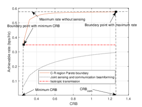
Figure 1: The C-R region with $K=35$.

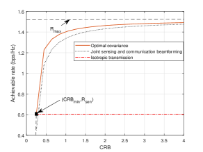
Figure 2: The C-R region with $K=3$.

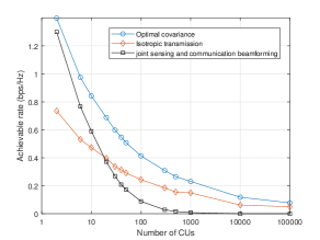
Figure 3: The achievable rate versus the number $K$ of CUs.

VI Conclusion

This paper studied the fundamental CRB-rate tradeoff in a multi-antenna multicast channel with ISAC. We characterized the Pareto boundary of the C-R region via maximizing the communication rate subject to a new maximum CRB constraint, for which the optimal transmit covariance solution was presented in semi-closed form. It was shown that optimal full-rank transmit covariance can be decomposed into two parts over communication and sensing subchannels, respectively, with different power allocation strategies. We also presented a practical joint communication and sensing beamforming. Numerical results were presented to show the C-R region under the optimal covariance and joint beamforming. How to extend the design to the cases with multi-antenna CUs and/or multi-group multicast channels with ISAC is interesting research directions that are worth pursuing in future.

Appendix A Proof of Lemma 1

First, consider the case with $\lambda_{1}=0$, in which problem (17) is equivalent to minimizing $\mathrm{tr}(\boldsymbol{A}(\lambda_{2},\{\mu_{k}\})\boldsymbol{S}_{x})$. Recall that $\boldsymbol{A}(\lambda_{2},\{\mu_{k}\})\succeq\boldsymbol{0}$ and $\boldsymbol{S}_{x}\succeq\boldsymbol{0}$. It is thus evident that any $\boldsymbol{S}_{x}^{*}$ satisfying $\boldsymbol{A}(\lambda_{2},\{\mu_{k}\})\boldsymbol{S}_{x}^{*}=\boldsymbol{0}$ is optimal.

Next, we consider the case with $\lambda_{1}>0$. As the EVD of $\boldsymbol{A}(\lambda_{2},\{\mu_{k}\})$ is $\boldsymbol{A}(\lambda_{2},\{\mu_{k}\})=\boldsymbol{U}\boldsymbol{\Lambda}\boldsymbol{U}^{H}$ with $\boldsymbol{\Lambda}=\mathrm{diag}(\alpha_{1},\dots,\alpha_{N_{t}})$, we have $\mathrm{tr}(\boldsymbol{A}(\lambda_{2},\{\mu_{k}\})\boldsymbol{S}_{x})=\mathrm{tr}(\boldsymbol{\Lambda}\boldsymbol{U}^{H}\boldsymbol{S}_{x}\boldsymbol{U})$. We define

$$\tilde{\boldsymbol{S}_{x}}=\boldsymbol{U}^{H}\boldsymbol{S}_{x}\boldsymbol{U}{\text{~{}or~{}}}\boldsymbol{S}_{x}=\boldsymbol{U}\tilde{\boldsymbol{S}_{x}}\boldsymbol{U}^{H}.$$ (30)

It is easy to verify that $\mathrm{tr}(\boldsymbol{S}_{x}^{-1})=\mathrm{tr}(\tilde{\boldsymbol{S}_{x}}^{-1})$. Accordingly, it follows that

$$\mathrm{tr}(\boldsymbol{A}(\lambda_{2},\{\mu_{k}\})\boldsymbol{S}_{x})+\lambda_{1}\mathrm{tr}(\boldsymbol{S}_{x}^{-1})=\mathrm{tr}(\boldsymbol{\Lambda}\tilde{\boldsymbol{S}_{x}})+\lambda_{1}\mathrm{tr}(\tilde{\boldsymbol{S}_{x}}^{-1}),$$

and problem (17) can be equivalently expressed as

$$\underset{\tilde{\boldsymbol{S}}_{x}\succeq\boldsymbol{0}}{\min}\mathrm{tr}(\boldsymbol{\Lambda}\tilde{\boldsymbol{S}_{x}})+\lambda_{1}\mathrm{tr}(\tilde{\boldsymbol{S}_{x}}^{-1}).$$ (31)

Then we have the following lemma.

Lemma 3.

For a positive semidefinite matrix $\boldsymbol{B}\in\mathbb{C}^{M\times M}$ with the $(m,n)$-th entry being $b(m,n),$ it holds that

$$\mathrm{tr}(\boldsymbol{B}^{-1})\geq\sum_{i=1}^{M}\frac{1}{b(i,i)},$$

where the equality is attained if and only if $\boldsymbol{B}$ is diagonal.

Proof.

See [22, Appendix I]. ∎

Based on Lemma 3, it follows that the optimal solution of $\tilde{\boldsymbol{S}_{x}}$ to problem (31) should be diagonal. As a result, we express $\tilde{\boldsymbol{S}_{x}}=\mathrm{diag}(\tilde{\beta}_{1},\dots,\tilde{\beta}_{N_{t}})$ with $\tilde{\beta}_{i}\geq 0,\forall i\in\{1,\ldots,N_{t}\}$. Accordingly, problem (31) is reduced as

$$\underset{{\{\tilde{\beta}_{i}\geq 0\}}}{\min}\sum_{i=1}^{N_{t}}\alpha_{i}\tilde{\beta}_{i}+\lambda_{1}\sum_{i=1}^{N_{t}}\frac{1}{\tilde{\beta}_{i}}.$$ (32)

It is clear that the optimal solution to problem 32 is given by

$$\tilde{\beta}_{i}^{*}\left\{\begin{array}[]{ll}=\lambda_{1}^{1/2}\alpha_{i}^{-1/2}&{\text{if~{}}}\alpha_{i}>0\\ \rightarrow\infty&{\text{if~{}}}\alpha_{i}=0\end{array}\right.,\forall i\in\{1,\ldots,N_{t}\}.$$ (35)

By combining (30), Lemma 3, and (35), we have the optimal solution to problem (17) as $\boldsymbol{S}_{x}^{*}=\lambda_{1}^{1/2}\boldsymbol{U}^{H}{\boldsymbol{\Sigma}}\boldsymbol{U},$ where ${\boldsymbol{\Sigma}}=\mathrm{diag}(\beta_{1}^{*},\dots,\beta_{N_{t}}^{*})$ with $\beta_{i}=\tilde{\beta}_{i}^{*}/\lambda_{1}^{1/2},$ $\forall i\in\{1,\ldots,N_{t}\}$. This thus completes the proof.

References

• [1] F. Liu, Y. Cui, C. Masouros, J. Xu, T. X. Han, Y. C. Eldar, and S. Buzzi, “Integrated sensing and communications: Towards dual-functional wireless networks for 6G and beyond,” IEEE J. Sel. Areas Commun., vol. 40, no. 6, pp. 1728–1767, Jun. 2022.
• [2] R. W. Heath and A. Lozano, Foundations of MIMO Communication.   Cambridge University Press, 2018.
• [3] A. M. Haimovich, R. S. Blum, and L. J. Cimini, “MIMO radar with widely separated antennas,” IEEE Signal Process. Mag., vol. 25, no. 1, pp. 116–129, Dec. 2007.
• [4] J. Li and P. Stoica, “MIMO radar with colocated antennas,” IEEE Signal Process. Mag., vol. 24, no. 5, pp. 106–114, Sep. 2007.
• [5] F. Liu, L. Zhou, C. Masouros, A. Li, W. Luo, and A. Petropulu, “Toward dual-functional radar-communication systems: Optimal waveform design,” IEEE Trans. Signal Process., vol. 66, no. 16, pp. 4264–4279, Aug. 2018.
• [6] X. Liu, T. Huang, N. Shlezinger, Y. Liu, J. Zhou, and Y. C. Eldar, “Joint transmit beamforming for multiuser MIMO communications and MIMO radar,” IEEE Trans. Signal Process., vol. 68, pp. 3929–3944, Jun. 2020.
• [7] H. Hua, J. Xu, and T. X. Han, “Transmit beamforming optimization for integrated sensing and communication,” in Proc. IEEE Global Commun. Conf. (GLOBECOM), 2021, pp. 01–06.
• [8] Z. Wang, Y. Liu, X. Mu, Z. Ding, and O. A. Dobre, “NOMA empowered integrated sensing and communication,” IEEE Commun. lett., vol. 26, no. 3, pp. 677–681, Mar. 2022.
• [9] L. Yin, Y. Mao, O. Dizdar, and B. Clerckx, “Rate-splitting multiple access for 6G–Part II: Interplay with integrated sensing and communications,” arXiv preprint arXiv:2205.02462, 2022.
• [10] A. Liu, Z. Huang, M. Li, Y. Wan, W. Li, T. X. Han, C. Liu, R. Du, D. K. P. Tan, J. Lu et al., “A survey on fundamental limits of integrated sensing and communication,” IEEE Commun. Surveys Tuts., vol. 24, no. 2, pp. 994–1034, 2nd Quart. 2022.
• [11] F. Liu, Y.-F. Liu, A. Li, C. Masouros, and Y. C. Eldar, “Cramér-Rao bound optimization for joint radar-communication beamforming,” IEEE Trans. Signal Process., vol. 70, pp. 240–253, Dec. 2021.
• [12] Y. Xiong, F. Liu, Y. Cui, W. Yuan, and T. X. Han, “Flowing the information from Shannon to Fisher: Towards the fundamental tradeoff in ISAC,” arXiv preprint arXiv:2204.06938, 2022.
• [13] H. Hua, X. Song, Y. Fang, T. X. Han, and J. Xu, “MIMO integrated sensing and communication with extended target: CRB-rate tradeoff,” arXiv preprint arXiv:2205.14050, 2022.
• [14] N. Jindal and Z.-Q. Luo, “Capacity limits of multiple antenna multicast,” in Proc. IEEE ISIT., 2006, pp. 1841–1845.
• [15] P. Stoica, J. Li, and Y. Xie, “On probing signal design for MIMO radar,” IEEE Trans. Signal Process., vol. 55, no. 8, pp. 4151–4161, Aug. 2007.
• [16] S. M. Kay, Fundamentals of Statistical Signal Processing: Estimation Theory.   Prentice-Hall, Inc., 1993.
• [17] S. Boyd and L. Vandenberghe, Convex Optimization.   Cambridge University Press, 2004.
• [18] S. Boyd, “Ellipsoid method,” May. 2014. [Online]. Available: https://web.stanford.edu/class/ee364b/lectures/ellipsoid_method_notes.pdf
• [19] M. Mohseni, R. Zhang, and J. M. Cioffi, “Optimized transmission for fading multiple-access and broadcast channels with multiple antennas,” IEEE J. Sel. Areas Commun., vol. 24, no. 8, pp. 1627–1639, Aug. 2006.
• [20] M. Grant and S. Boyd, “CVX: Matlab software for disciplined convex programming, version 2.1,” Mar. 2014. [Online]. Available: http://cvxr.com/cvx
• [21] N. D. Sidiropoulos, T. N. Davidson, and Z.-Q. Luo, “Transmit beamforming for physical-layer multicasting,” IEEE Trans. Signal Process., vol. 54, no. 6, pp. 2239–2251, Jun. 2006.
• [22] S. Ohno and G. B. Giannakis, “Capacity maximizing MMSE-optimal pilots for wireless OFDM over frequency-selective block Rayleigh-fading channels,” IEEE Trans. Inf. Theory, vol. 50, no. 9, pp. 2138–2145, Sep. 2004.