GlanceNets: Interpretable, Leak-proof
Concept-based Models

Abstract

There is growing interest in concept-based models (CBMs) that combine high-performance and interpretability by acquiring and reasoning with a vocabulary of high-level concepts. A key requirement is that the concepts be interpretable. Existing CBMs tackle this desideratum using a variety of heuristics based on unclear notions of interpretability, and fail to acquire concepts with the intended semantics. We address this by providing a clear definition of interpretability in terms of alignment between the model’s representation and an underlying data generation process, and introduce GlanceNets, a new CBM that exploits techniques from disentangled representation learning and open-set recognition to achieve alignment, thus improving the interpretability of the learned concepts. We show that GlanceNets, paired with concept-level supervision, achieve better alignment than state-of-the-art approaches while preventing spurious concepts from unintentionally affecting its predictions. The code is available at https://github.com/ema-marconato/glancenet.

1 Introduction

Concept-based models (CBMs) are an increasingly popular family of classifiers that combine the transparency of white-box models with the flexibility and accuracy of regular neural nets [1, 2, 3, 4, 5]. At their core, all CBMs acquire a vocabulary of concepts capturing high-level, task-relevant properties of the data, and use it to compute predictions and produce faithful explanations of their decisions [6].

The central issue in CBMs is how to ensure that the concepts are semantically meaningful and interpretable for (sufficiently expert and motivated) human stakeholders. Current approaches struggle with this. One reason is that the notion of interpretability is notoriously challenging to pin down, and therefore existing CBMs rely on different heuristics—such as encouraging the concepts to be sparse [1], orthonormal to each other [5], or match the contents of concrete examples [3]—with unclear properties and incompatible goals. A second, equally important issue is concept leakage, whereby the learned concepts end up encoding spurious information about unrelated aspects of the data, making it hard to assign them clear semantics [7]. Notably, even concept-level supervision is insufficient to prevent leakage [8].

Prompted by these observations, we define interpretability in terms of alignment: learned concepts are interpretable if they can be mapped to a (partially) interpretable data generation process using a transformation that preserves semantics. This is sufficient to unveil limitations in existing strategies, build an explicit link between interpretability and disentangled representations, and provide a clear and actionable perspective on concept leakage. Building on our analysis, we also introduce GlanceNets (aliGned LeAk-proof coNCEptual Networks), a novel class of CBMs that combine techniques from disentangled representation learning [9] and open-set recognition (OSR) [10] to actively pursue alignment – and guarantee it under suitable assumptions – and avoid concept leakage.

Contributions: Summarizing, we: (i) Provide a definition of interpretability as alignment that facilitates tapping into ideas from disentangled representation learning; (ii) Show that concept leakage can be viewed from the perspective of out-of-distribution generalization; (iii) Introduce GlanceNets, a novel class of CBMs that acquire interpretable representations and are robust to concept leakage; (iv) Present an extensive empirical evaluation showing that GlanceNets are as accurate as state-of-the-art CBMs while attaining better interpretability and avoiding leakage.

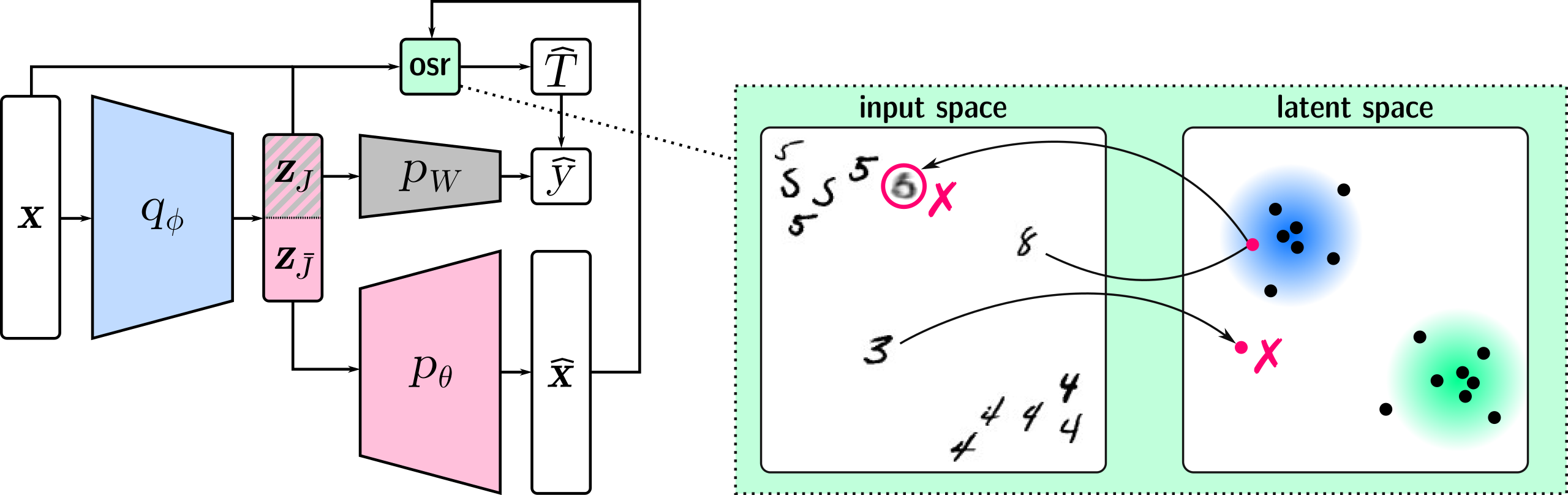
Figure 1: Left: Architecture of GlanceNets showing the encoder $q_{\phi}$, decoder $p_{\theta}$, classifier $p_{W}$, and open-set recognition step. Right: At test time, GlanceNets prevent leakage by identifying and rejecting out-of-distribution inputs using a combined strategy, shown here for a model trained on digits “$4$” and “$5$” only: the “$3$” is rejected as its embedding falls far away from prototypes of the two training classes (colored blobs), while the “$8$” is rejected as its reconstruction loss is too large.

2 Concept-based Models: Interpretability and Concept Leakage

Concept-based models (CBMs) comprise two key elements: (i) A learned vocabulary of $k$ high-level concepts meant to enable communication with human stakeholders [11], and (ii) a simulatable [12] classifier whose predictions depend solely on those concepts. Formally, a CBM $f:\mathbb{R}^{d}\to[c]$, with $[c]:=\{1,\ldots,c\}$, maps instances $\bm{\mathrm{x}}$ to labels $y$ by measuring how much each concept activates on the input, obtaining an activation vector $\bm{\mathrm{z}}(\bm{\mathrm{x}}):=(z_{1}(\bm{\mathrm{x}}),\ldots,z_{k}(\bm{\mathrm{x}}))^{T}\in\mathbb{R}^{k}$, aggregating the activations into per-class scores $s_{y}(\bm{\mathrm{x}})$ using a linear map [1, 3, 5], and then passing these through a softmax, i.e.,

$$\textstyle s_{y}(\bm{\mathrm{x}}):=\sum_{j}w_{yj}\cdot z_{j}(\bm{\mathrm{x}}),\qquad p(y\ |\ \bm{\mathrm{x}}):=\mathrm{softmax}(\bm{\mathrm{s}}(\bm{\mathrm{x}}))_{y}.$$ (1)

Each weight $w_{yj}\in\mathbb{R}$ encodes the relevance of concept $z_{j}$ for class $y$. The activations themselves are computed in a black-box manner, often leveraging pre-trained embedding layers, but learned so as to capture interpretable aspects of the data using a variety of heuristics, discussed below.

Now, as long as the concepts are interpretable, it is straightforward to extract human understandable local explanations disclosing how different concepts contributed to any given decision $(\bm{\mathrm{x}},y)$ by looking at the concept activations and their associated weights, thus abstracting away the underlying computations. This yields explanations of the form $\{(w_{yj},\,z_{j}(\bm{\mathrm{x}})):j\in[k]\}$ that can be readily summarized and visualized [13, 14]. Importantly, the score of class $y$ is conditionally independent from the input $\bm{\mathrm{x}}$ given the corresponding explanation, i.e., $s_{y}(\bm{\mathrm{x}})\mathrel{\text{\scalebox{1.07}{$\perp\mkern-10.0mu\perp$}}}\bm{\mathrm{x}}\mid\mathcal{E}(\bm{\mathrm{x}},y)$, ensuring that the latter is faithful to the model scores. GlanceNets inherit all of these features.

Heuristics for interpretability. Crucially, CBMs are only interpretable insofar as their concepts are. Existing approaches implement special mechanisms to this effect, often pairing a traditional classification loss (such as the cross-entropy loss) with an auxiliary regularization term.

Alvarez-Melis and Jaakkola [1] acquire concepts using an autoencoder augmented with a sparsification penalty encouraging distinct concepts to activate on different instances. Chen et al. [5] apply geometric transforms to learn mutually orthonormal concepts that thus encode complementary information and attain comparable activation ranges. These mechanisms – sparsity and orthogonality, respectively – alone cannot prevent capturing features that are not semantic in nature.

A second group of CBMs tackle this issue by constraining the concepts to match concrete cases, in the hope that these are better aligned with human intuition [15]. For instance, prototype classification networks [2], part-prototype networks [3], and related approaches [16, 17, 18] model concepts using prototypes in embedding space that perfectly match training examples or parts thereof. Depending on the embedding space, which ultimately determines the distance to the prototypes, concepts learned this way may activate on elements unrelated to the example they match, leading to unclear semantics [19].

Closest to our work, concept bottleneck models (CBNMs) [20, 4] align the concepts using concept-level supervision – possibly obtained from a separate source, like ImageNet [21] – either sequentially or in tandem with the top-level dense layer. From a statistical perspective, this seems perfectly sensible: if the supervision is unbiased and comes in sufficient quantity, and the model has enough capacity, this strategy appears to guarantee the learned and ground-truth concepts to match.

Concept leakage in concept-bottleneck models. Unfortunately, concept-level supervision is not sufficient to guarantee interpretability. Mahinpei et al. [7] have demonstrated that concepts acquired by CBNMs pick up spurious properties of the data. In their experiment, they learn two concepts $z_{4}$ and $z_{5}$, meant to represent the $4$ and $5$ MNIST digits, using concept-level supervision, and then show that – surprisingly – these concepts can be used to classify all other digits (i.e., MNIST images that are neither $4$’s nor $5$’s) as even or odd significantly better than random guessing. This phenomenon, whereby learned concepts unintentionally capture information about unobserved concepts, is known as concept leakage.

Intuitively, leakage occurs because in CBNMs the concepts end up unintentionally capturing distributional information about unobserved aspects of the input, failing to provide well-defined semantics. However, a clear definition of leakage is missing, and so are strategies to prevent it. In fact, separating concept learning from classification and increasing the amount of supervision for the observed concepts (here, $4$ and $5$) is not enough [8]. A key contribution of our paper is showing that leakage can be understood from the perspective of domain shift and dealt with using open-set recognition [10].

3 Disentangling Interpretability and Concept Leakage

The main issue with heuristics used by CBMs is that they are based on unclear notions of interpretability. In order to develop effective algorithms, we propose to view interpretability as a form of alignment between the machine’s representation and that of its user. This enables us to identify conditions under which interpretability can be achieved, build links to well-understood properties of representations, and leverage state-of-the-art learning strategies.

Figure 2: The data generation process.

Interpretability. We henceforth focus on the (rather general) generative process shown in Fig. 2: the observations $\bm{\mathrm{X}}\in\mathbb{R}^{d}$ are caused by $n$ generative factors $\bm{\mathrm{G}}\in\mathbb{R}^{n}$, themselves caused by a set of confounds $\bm{\mathrm{C}}$ (including the label $Y$ [22]). Notice that the generative factors can be statistically dependent due to the confounds $\bm{\mathrm{C}}$, but as noted by Suter et al. [23], the total causal effect [24, Def. 6.12] between $G_{i}$ and $G_{j}$ is zero for all $i\neq j$. The generative factors capture all information necessary to determine the observation [23, 25], so the goal is to learn concepts $\bm{\mathrm{Z}}\in\mathbb{R}^{k}$ that recover them. The variable $T$ is also a confounding factor, but it is kept separate from $\bm{\mathrm{C}}$ as it relates to concept leakage, and will be formally introduced later on.

We posit that a (learned) representation is only interpretable if it supports symbolic communication between the model and the user, in the sense that it shares the same (or similar enough) semantics to the user’s representation. The latter is however generally unobserved. We therefore make a second, critical assumption that some of the generative factors $\bm{\mathrm{G}}_{I}\subseteq\bm{\mathrm{G}}$ are interpretable to the user, meaning that they can be used as a proxy for the user’s internal representation. Naturally, not all generative factors are interpretable [26], but in many applications some of them are. For instance, in dSprites [27] the generative factors encode the position, shape and color of a 2D object, and in CelebA [28] the hair color and nose size of a celebrity. Human observers have a good grasp of such concepts.

Interpretability as alignment. Under this assumption, if the variables $\bm{\mathrm{Z}}_{J}\subseteq\bm{\mathrm{Z}}$ are aligned to the generative factors $\bm{\mathrm{G}}_{I}$ by a map $\alpha:\bm{\mathrm{g}}\mapsto\bm{\mathrm{z}}_{J}$ that preserves semantics, they are themselves interpretable. Now, defining what a semantics-preserving map should look like is challenging, but constructing one is not: the identity is clearly one such map, and so are maps that permute the indices and independently rescale the individual variables. One desirable property is that $\alpha$ does not “mix” multiple $G$’s into a single $Z$. E.g., if $Z$ blends together head tilt, hair color, and nose size, users will have trouble pinning down what it means. This property can be formalized in terms of disentanglement [29, 23, 9]. This is however insufficient: we wish the map between $G_{i}$ and its associated factor $Z_{j}$ to be “simple”, so as to conservatively guarantee that it preserves semantics. This makes alignment strictly stronger than disentanglement.

Motivated by these desiderata, we say that $\bm{\mathrm{Z}}_{J}$ is aligned to $\bm{\mathrm{G}}_{I}$ if it satisfies:

• Disentanglement. There exists an injective map between indices $\pi:[n_{I}]\to[k]$, where $[n_{I}]$ identifies the subset of generative factors indexes in $\bm{\mathrm{G}}_{I}$, such that, for all $i,i^{\prime}\in[n_{I}]$, $i\neq i^{\prime}$, and $j=\pi(i)$, it holds that fixing $G_{i}$ is enough to fix $Z_{j}$ regardless of the value taken by the other generative factors $G_{i^{\prime}}$, and

• Monotonicity. The map $\alpha$ can be written as $\alpha(\bm{\mathrm{g}})=(\mu_{1}(g_{\pi(1)}),\ldots,\mu_{n}(g_{\pi(n_{I})}))^{T}$, where the $\mu_{i}$’s are monotonic transformations. This holds, for instance, for linear transformations of the form $A\ (g_{\pi(1)},\ldots,g_{\pi(n_{I})})^{T}$ , where $A\in\mathbb{R}^{n_{I}\times k}$ is a matrix with no non-zero off-diagonal entries. This second requirement can be relaxed depending on the application.

Notice that we do not require each $G_{i}$ to map to a single $Z_{j}$ (a property known as completeness [29]): $\bm{\mathrm{Z}}_{J}$ is interpretable even if it contains multiple – perhaps slightly different, but aligned – transformations of the same $G_{i}$.

Measuring alignment with DCI. Disentanglement can be measured in a number of ways [30], but most of them provide little information about how simple the map $\alpha$ is. In order to estimate alignment, we repurpose DCI, a measure of disentanglement introduced by Eastwood and Williams [29], see also Appendix B. According to this metric, a representation $\bm{\mathrm{Z}}_{J}$ is disentangled if there exists a regressor that, given $\bm{\mathrm{z}}_{J}$, can predict $\bm{\mathrm{g}}_{I}$ with high accuracy using few $z_{i}$’s to predict each $g_{i}$. Following [29], we use a linear regressor with parameters $B\in\mathbb{R}^{k\times n_{I}}$ on the test set – assuming that it is annotated with the interpretable generative factors and corresponding learned representations – and then measure how diffuse the weights associated to each latent factor are. We do this by normalizing them and computing their average Shannon entropy over all $G_{i}$’s, i.e.,

$$\textstyle-\sum_{j\in[k]}\rho_{j}\left(\sum_{i\in[n_{I}]}\bar{b}_{ji}\log\bar{b}_{ji}\right),\quad\text{where $\bar{b}_{ji}=b_{ji}/\sum_{j^{\prime}\in[k]}b_{j^{\prime}i}$}\quad\text{and}\quad\rho_{j}=\sum_{i}b_{ji}/\sum_{j^{\prime}i}b_{j^{\prime}i}$$ (2)

Hence, DCI gauges the degree of mixing that a linear map can attain using the learned representation $\bm{\mathrm{Z}}$, and as such it indirectly measures alignment, with $B$ approximating the inverse of $A$.

Achieving alignment with concept-level supervision. It has been shown that disentanglement cannot be achieved in the purely unsupervised setting [31]. This immediately entails that alignment is also impossible in that setting, highlighting a core limitation of approaches like self-explainable neural networks [1]. However, disentanglement can be attained if supervision about the generative factors is available, even only for a small percentage of the examples [32]. As a matter of fact, supervision is used in representation learning to achieve identifiability, a stronger condition than – and that entails both of – disentanglement and alignment [33]. Thus, following CBNMs, we seek alignment by leveraging concept-level supervision.

Interpretability and concept leakage. Intuitively, concept leakage occurs when a model is trained on a data set on which:

• Some generative factors $\bm{\mathrm{G}}_{V}\subset\bm{\mathrm{G}}$ vary, while the others $\bm{\mathrm{G}}_{F}=\bm{\mathrm{G}}\setminus\bm{\mathrm{G}}_{V}$ are fixed, and

• The two groups of factors are statistically dependent.

For instance, in the even vs. odd experiment $4$ and $5$ play the role of $\bm{\mathrm{G}}_{V}$ and the other digits of $\bm{\mathrm{G}}_{F}$. CBNMs with access to supervision on $\bm{\mathrm{G}}_{V}$ tend to acquire a latent representation that approximates these factors. But, because of (ii), this representation correlates with the fixed factors $\bm{\mathrm{G}}_{F}$. This immediately explains why additional supervision on $\bm{\mathrm{G}}_{V}$ cannot prevent leakage, but rather has the opposite effect: the better a latent representation matches $\bm{\mathrm{G}}_{V}$, the more information it conveys about $\bm{\mathrm{G}}_{F}$.

In contrast with previous assessments [7, 8], we observe that this phenomenon can be viewed as a special form of domain shift: the training examples are sampled from a ground-truth distribution $p(\bm{\mathrm{X}},\bm{\mathrm{G}}\mid T=1)$ in which $\bm{\mathrm{G}}_{F}$ is approximately fixed, e.g., $p(\bm{\mathrm{G}}_{F}\mid T=1)=\delta(\bm{\mathrm{g}}_{F}^{\prime})$ for some vector $\bm{\mathrm{g}}_{F}^{\prime}$, while in the test set, the data is sampled from a different distribution $p(\bm{\mathrm{X}},\bm{\mathrm{G}}\mid T=0)$ in which $\bm{\mathrm{G}}_{F}$ is no longer fixed. In the MNIST task, for instance, when $T=1$ no concept besides $4$ and $5$ can occur, while all concepts except $4$ and $5$ can occur when $T=0$. Here, $T\in\{0,1\}$ selects between training and test distribution, see Fig. 2. Now, CBMs have no strategy to cope with domain shift and thus cannot disambiguate between known training and unknown test concepts.

Motivated by this, we propose then to tackle concept leakage by designing a CBM specifically equipped with strategies for detecting – at inference time – instances that do not belong to the training distribution using OSR [10]. The idea is to estimate the value of the variable $T$ at inference time, essentially predicting whether an input was sampled from a distribution similar enough to the training distribution, and therefore can be handled by a model learned on this distribution, or not. This strategy proves very effective in practice, as shown by our empirical evaluation (Section 5.2).

4 Addressing Alignment and Leakage with GlanceNets

GlanceNets combine a VAE-like architecture [34, 35] for learning disentangled concepts with a prior and classifier designed for open-set prediction [36]. In order to accommodate for non-interpretable factors, the latent representation of GlanceNets $\bm{\mathrm{Z}}$ is split into two: (i) $k$ concepts $\bm{\mathrm{Z}}_{J}$, aligned to the interpretable generative factors $\bm{\mathrm{G}}_{I}$, that are used for prediction, and (ii) $\bar{k}$ opaque factors $\bm{\mathrm{Z}}_{\bar{J}}$ that are only used for reconstruction. Specifically, a GlanceNet comprises an encoder $q_{\phi}(\bm{\mathrm{Z}}\mid\bm{\mathrm{X}})$ and a decoder $p_{\theta}(\bm{\mathrm{X}}\mid\bm{\mathrm{Z}})$, both parameterized by deep neural networks, as well as a classifier $p_{W}(Y\mid\bm{\mathrm{Z}}_{J})$ feeding off the interpretable concepts only. The overall architecture is shown in Fig. 1.

Following other CBMs, the classifier is implemented using a dense layer with parameters $W\in\mathbb{R}^{v\times k}$ followed by a softmax activation, i.e., $p_{W}(Y\mid\bm{\mathrm{z}}_{J}):=\mathrm{softmax}(W\bm{\mathrm{z}}_{J})$, and the most likely label is used for prediction. The class distribution is obtained by marginalizing over the encoder’s distribution:

$$p(Y\mid\bm{\mathrm{x}}):=\mathbb{E}_{q_{\phi}(\bm{\mathrm{z}}\mid\bm{\mathrm{x}})}[p(Y\mid\bm{\mathrm{z}},\bm{\mathrm{x}})]=\mathbb{E}_{q_{\phi}(\bm{\mathrm{z}}\mid\bm{\mathrm{x}})}[p_{W}(Y\mid\bm{\mathrm{z}}_{J})]$$ (3)

Equality holds because $Y\mathrel{\text{\scalebox{1.07}{$\perp\mkern-10.0mu\perp$}}}\bm{\mathrm{X}}\mid\bm{\mathrm{Z}}_{J}$. In order to expedite the computation, we follow the general practice of approximating the integral as $\mathrm{softmax}(W\,\mathbb{E}_{q_{\phi}(\bm{\mathrm{z}}\mid\bm{\mathrm{x}})}[\bm{\mathrm{z}}_{J}])=\mathrm{softmax}(W[\bm{\mathrm{\mu}}_{\phi}(\bm{\mathrm{x}})]_{J})$.

In contrast to regular VAEs, GlanceNets associate each class to a prototype in latent space through the prior $p(\bm{\mathrm{Z}}\mid\bm{\mathrm{Y}})$, which is conditioned on the class and modelled as a mixture of gaussians with one component per class. The encoder, decoder, and prior are fit on data so as to maximize the evidence lower bound (ELBO) [37], defined as $\mathbb{E}_{p_{D}(\bm{\mathrm{x}},y)}[\mathcal{L}(\theta,\bm{\mathrm{x}},y;\beta)]$ with:

$$\mathcal{L}(\theta,\bm{\mathrm{x}},y;\beta):=\mathbb{E}_{q_{\phi}(\bm{\mathrm{z}}\mid\bm{\mathrm{x}})}[\log p_{\theta}(\bm{\mathrm{x}}\mid\bm{\mathrm{z}})+\log p_{W}(y\mid\bm{\mathrm{z}}_{J})]-\beta\cdot\mathsf{KL}(q_{\phi}(\bm{\mathrm{z}}\mid\bm{\mathrm{x}})\,\|\,p(\bm{\mathrm{z}}\,|\,y))$$ (4)

Here, $p_{D}(\bm{\mathrm{x}},y)$ is the empirical distribution of the training set $D=\{(\bm{\mathrm{x}}_{i},y_{i}):i=1,\ldots,m\}$. The first term of Eq. 4 is the likelihood of an example after passing it through the encoder distribution.

The second term penalizes the latent vectors based on how much their distribution differs from the prior and encourages disentanglement. As mentioned in Section 3, learning disentangled representations is impossible in the unsupervised i.i.d. setting [31]. Following Locatello et al. [32], and similarly to CBNMs, we assume access to a (possibly separate) data set $\widetilde{D}=\{(\bm{\mathrm{x}}_{\ell},\bm{\mathrm{g}}_{I,\ell})\}$ containing supervision about the interpretable generative factors $\bm{\mathrm{G}}_{I}$ and integrate it into the ELBO by replacing the per-example loss $\mathcal{L}$ in Eq. 4 with:

$${\mathbb{E}_{p_{\mathcal{D}}(\bm{\mathrm{x}},y)}}\big{[}\mathcal{L}(\theta,\bm{\mathrm{x}},y;\beta)\big{]}+\gamma\cdot\mathbb{E}_{p_{\tilde{D}}(\bm{\mathrm{x}},\bm{\mathrm{g}})}\mathbb{E}_{q_{\phi}(\bm{\mathrm{z}}\mid\bm{\mathrm{x}})}\big{[}\Omega(\bm{\mathrm{z}},\bm{\mathrm{g}})\big{]}$$ (5)

where $\gamma>0$ controls the strength of the concept-level supervision. Following [32], the term $\Omega(\bm{\mathrm{z}},\bm{\mathrm{g}})$ penalizes encodings sampled from $q_{\phi}(\bm{\mathrm{z}}\,|\,\bm{\mathrm{x}})$ for differing from the annotation $\bm{\mathrm{g}}$. Specifically, we implement this term using the average cross-entropy loss $\Omega(\bm{\mathrm{z}},\bm{\mathrm{g}}):=-\sum_{k}g_{k}\log\sigma(z_{k})+(1-g_{k})\log(1-\sigma(z_{k}))$, where the annotations $g_{k}$ are rescaled to lie in $[0,1]$ and $\sigma$ is the sigmoid function.

Dealing with concept leakage. In order to tackle concept leakage, GlanceNets integrate the OSR strategy of Sun et al. [36], indicated in Fig. 1 by the “osr” block. This strategy identifies out-of-class inputs by considering the class prototype $\mu_{y}:=\mathbb{E}_{p(\bm{\mathrm{z}}|y)}[\bm{\mathrm{z}}]$ in $\mathbb{R}^{k}$ defined by the prior distribution and the decoder $p_{\theta}(\bm{\mathrm{x}}|\bm{\mathrm{z}})$. Recall that the prior is fit jointly with the encoder, decoder, and classifier by optimizing the ELBO. Once learned, a GlanceNet uses the training data to estimate: (i) a distance threshold $\eta_{y}$, which defines a spherical subset in the latent space ${\mathcal{B}}_{y}=\{\bm{\mathrm{z}}:\,\lVert\mu_{y}-\bm{\mathrm{z}}\rVert<\eta_{y}$ } centered around the prototype of class $y$ (i.e., the mean of the corresponding Gaussian mixture component), and (ii) a maximum threshold on the reconstruction error $\eta_{thr}$. If new data points have reconstruction error above $\eta_{thr}$ or they do not belong to any subset ${\mathcal{B}}_{y}$, they are inferred as open-set instances, i.e., $\hat{T}=0$. In practice, we found that choosing the thresholds as to include 95% of training examples to work well in our experiments. Further details are available in Appendices A and C.

4.1 Benefits and Limitations

GlanceNets can naturally be combined with different VAE-based architectures for learning disentangled representations [38], including $\beta$-TCVAEs [39], InfoVAEs [40], DIP-VAEs [41], and JL1-VAEs [42]. Since our experiments already show substantial benefits for GlanceNets building on $\beta$-VAEs [43], we leave a detailed study of these extensions to future work.

Like CBNMs, GlanceNets foster alignment by leveraging supervision on the interpretable generative factors [32], possibly derived from an external data set [20]. However, GlanceNets can be readily adapted to a variety of different kinds of supervision used for VAE-based models, including partially annotated examples [26], group information [44], pairings [45, 46] and other kinds of weak supervision [47, 48], as well as feedback from a domain expert [49]. On the other hand, CBNMs are incompatible with these approaches.

One limitation inherited from VAEs by GlanceNets is the assumption that the interpretable generative factors are disentangled from each other [23]. In practice, GlanceNets work even when this does not hold (as in our even vs. odd experiment, see Section 5.2). However, one direction of future work is to integrate ideas from hierarchical disentanglement [50].

5 Empirical Evaluation

In this section, we present results on several tasks showing that GlanceNets outperform CBNMs [20] in terms of alignment and robustness to leakage, while achieving comparable prediction accuracy. All experiments were implemented using Python 3 and Pytorch [51] and run on a server with 128 CPUs, 1TiB RAM, and 8 A100 GPUs. GlanceNets were implemented on top of the disentanglement-pytorch [52] library. All alignment and disentanglement metrics were computed with disentanglement_lib [31]. Code for the complete experimental setup is available on GitHub at the link: https://github.com/ema-marconato/glancenet. Additional details on architectures and hyperparameters can also be found in the Supplementary Material.

	Accuracy	Alignment	Explicitness
dSprites
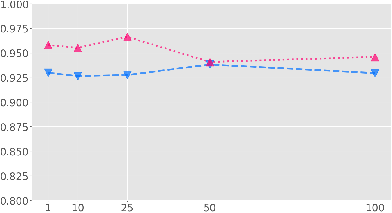
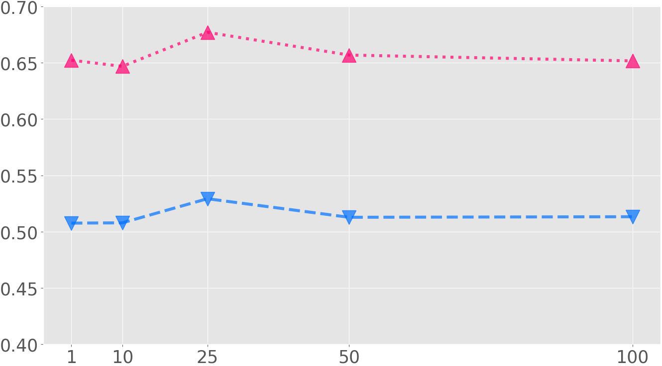
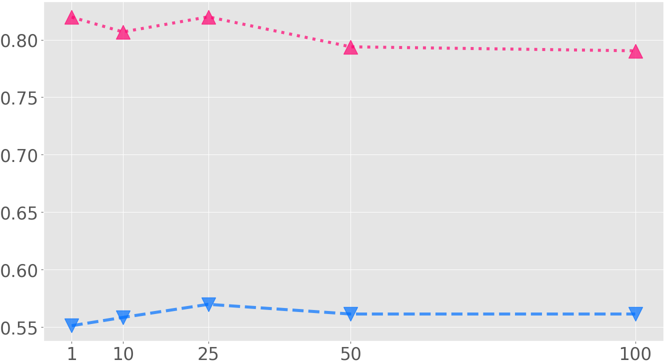
MPI3D
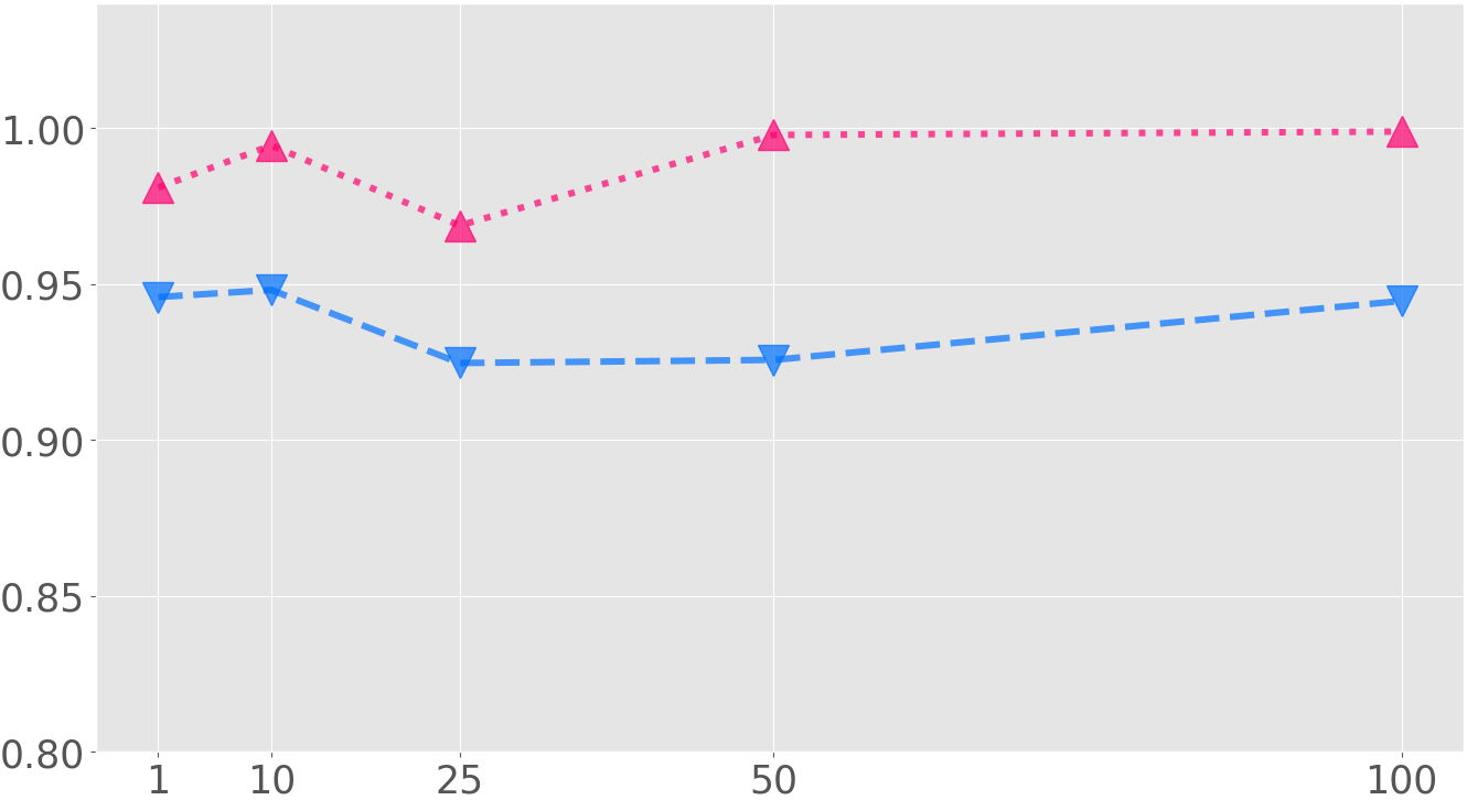
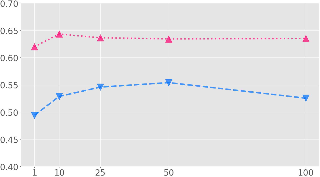
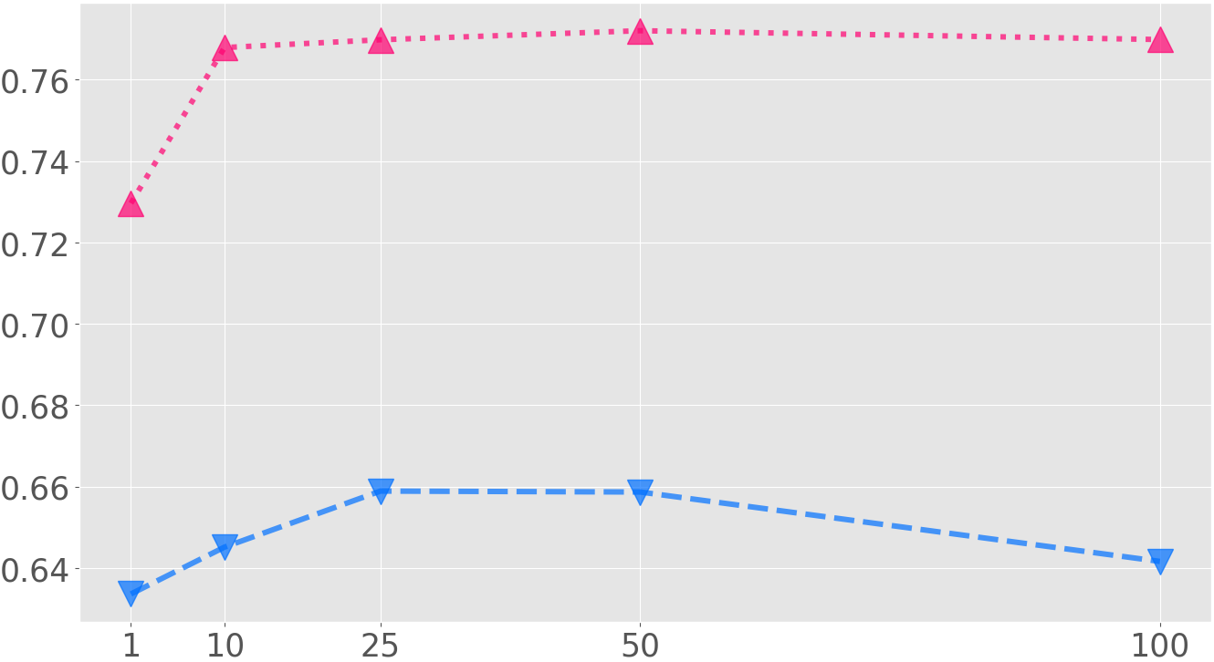
CelebA

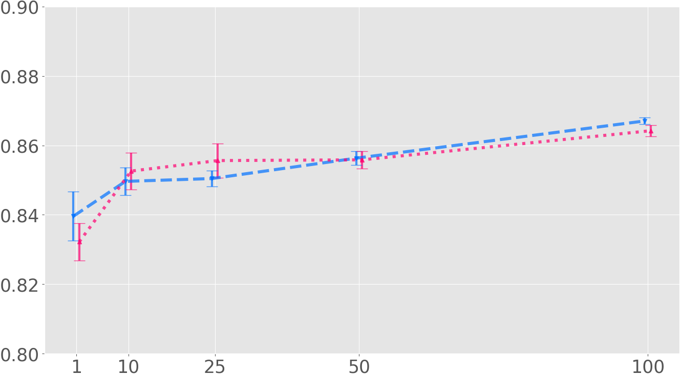
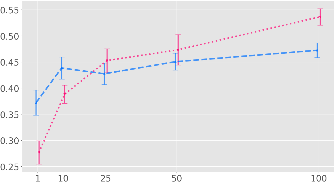
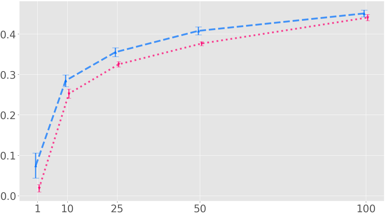
Figure 3: GlanceNets are better aligned than CBNMs. Each row is a data set and each column reports a different metric. The horizontal axes indicate the $\%$ of training examples for which supervision on the generative factors is provided. Remarkably, in all data sets GlanceNets achieve substantially better alignment than CBNMs for the same amount of supervision, and achieve comparable accuracy in $14$ cases out of $15$.

5.1 GlanceNets achieve better alignment than CBNMs

In a first experiment, we compared GlanceNets with CBNMs on three classification tasks for which supervision on the generative factors is available. In order to evaluate the impact of this supervision on the different competitors, we varied the amount of training examples annotated with it from $1\%$ to $100\%$. For each increment, we measured prediction performance using accuracy, and alignment using the linear variant of DCI [29] discussed in Section 3.

Data sets. We carried out our evaluation on two data sets taken from the disentanglement literature and a very challenging real-world data set. dSprites [27] consists of $64\times 64$ black-and-white images of sprites on a flat background, where each sprite is determined by one categorical and four generative factors, namely shape, size, rotation, position_x, and position_y. The images were obtained by discretizing and enumerating the generative factors, for a total of $3\times 6\times 40\times 32\times 32$ images. MPI3D [53] consists of $64\times 64$ RGB rendered images of 3D shapes held by a robotic arm. The generative factors are object_color, object_shape, object_size, camera_height, background_color, and the horizontal and vertical position of the arm. The data contains $6\times 6\times 2\times 3\times 4\times 40\times 40$ examples. CelebA [28] is a collection of $178\times 218$ RGB images of over 10k celebrities, converted to $64\times 64$ by first cropping them to $178\times 178$ and then rescaling. Images are annotated with 40 binary generative factors including hair color, presence of sunglasses, etc. Since we are interested in measuring alignment, we considered only those $10$ factors that CBNMs can fit well (in the Appendix). We also dropped all those examples for which hair color is not unique (e.g., annotated as both blonde and black), obtaining approx. $127k$ examples. CelebA is more challenging than dSprites and MPI3D, as it does not include all possible factor variations and the generative factors – although disentangled – are insufficient to completely determine the contents of the images. For dSprites and MPI3D, we used a random 80/10/10 train/validation/test split, while for CelebA we kept the original split [28].

We generated the ground-truth labels $y$ as follows. For dSprites, we labeled images according to a random but fixed linear separator defined over the continuous generative factors, chosen so as to ensure that the classes are balanced. For MPI3D and CelebA, we focused on the categorical factors instead. Specifically, we clustered all images using the algorithm of [54], for a total of $10$ and $4$ clusters for MPI3D and CelebA respectively, and then labeled all examples based on their reference cluster. This led to slightly unbalanced classes containing different percentages of examples, ranging from $5\%$ to $16\%$ in MPI3D and from $21\%$ to $29\%$ in CelebA.

Architectures. For dSprites and MPI3D, we implemented the encoder as a six layer convolutional neural net, while for CelebA we adapted the convolutional architecture of Ghosh et al. [55]. We employed a six layer convolutional architecture for the decoder in all cases, for simplicity, as changing it did not lead to substantial differences in performance. In all cases, as for all CBMs (see Section 2), the classifier was implemented as a dense layer followed by a softmax activation. The very same architectures were used for both GlanceNets and CBNMs, for fairness. For each data set, we chose the latent space dimension as the total number of generative factors, where categorical ones are one hot encoded. In particular, we used 7 latent factors for dSprites, 21 for MPI3D and 10 for CelebA. Further details are included in the Supplementary Material.

Results and discussion. The results of this first experiment are reported in Fig. 3. The behavior of both competitors on dSprites and MPI3D was extremely stable, owing to the fact that these data sets cover an essentially exhaustive set of variations for all generative factors, so we report their hold-out performance on the test set. Since for CelebA variance was non-negligible, we ran both methods $7$ times varying the random seed used to initialize the network and report the average performance across runs and its standard deviation.

In addition to alignment, we also report explicitness [29], which measures how well the linear regressor employed by DCI fits the generative factors. The higher, the better. Details on its evaluation are included in Suppl. Material.

The plots clearly show that, although the two methods achieve high and comparable accuracy in all settings, GlanceNets attain better alignment in all data sets and for all supervision regimes than CBNMs, with a single exception in CelebA using low values of supervision, for a total of $13$ wins out of $15$ cases. In all $disentanglement$ data sets, there is a clear margin between the alignment achieved by GlanceNets and that of CBNMs: performances vary up to maximum of 15% in dSprites, and a minumum of 8% in MPI3D. In CelebA, the gap is evident with full supervision (almost 8% of difference in alignment), and GlanceNets still attain overall better scores in the 25% and 50% regime. On the other hand, performance are lower, but comparable, with 10% supervision. The case at 1% refers to an extreme situation where both CBNMs and GlanceNets struggle to align with generative factors, as is clear also from the very low explicitness.

In dSprites and MPI3D, both GlanceNets and CBNMs quickly achieve very high alignment at $1\%$ supervision, as expected [32], whereas better results in CelebA are obtained with growing supervision. Also, both models display similar stability on this data set, as shown by the error bars in the plot.

5.2 GlanceNets are leak-proof

Next, we evaluated robustness to concept leakage in two scenarios that differ in whether the unobserved generative factors are disentangled with the observed ones or not, see Section 3. In both experiments, we compare GlanceNets with a CBNM and a modified GlanceNet where the OSR component has been removed (denoted CG-VAE).

Leakage due to unobserved entangled factors. We start by replicating the experiment of Mahinpei et al. [7]: the goal is to discriminate between even and odd MNIST images using a latent representation $\bm{\mathrm{Z}}=(Z_{4},Z_{5})$ obtained by training (with complete supervision on the generative factors) only on examples of $4$’s and $5$’s. Leakage occurs if the learned representation can be used to solve the prediction task better than random on a test set where all digits except $4$ and $5$ occur. During training, we use the digit label for conditioning the prior $p(\bm{\mathrm{Z}}\mid\bm{\mathrm{Y}})$ of the GlanceNet. More qualitative results are collected in Appendix D.

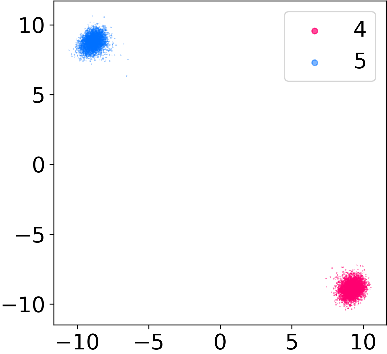
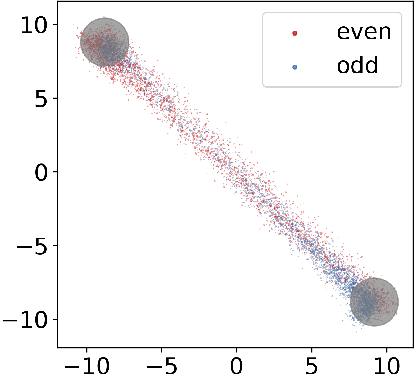
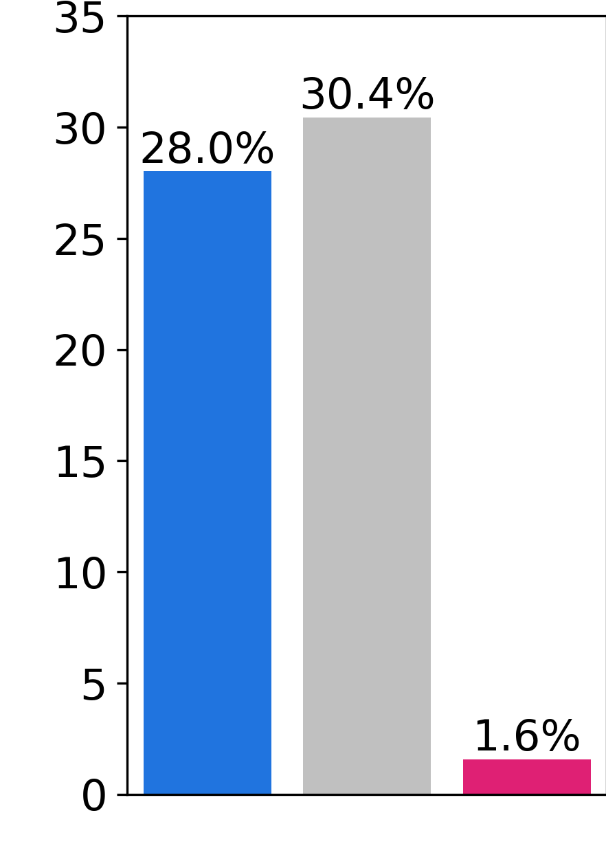
(a)	(b)	(c)

Figure 4: GlanceNets are leak-proof on MNIST. (a) Training set embedded by GlanceNet with $\beta=100$; axes indicate $z_{4}$ and $z_{5}$ and color the concept label, i.e., $4$ vs. $5$. (b) Latent representations of the test images, divided in even vs. odd. Every ball in light gray denotes the region $|\mu_{y}-\bm{\mathrm{z}}|<\eta_{y}$ for each class prototype $y$. For more details, refer to Section 3. (c) Information Leakage performances of the considered models: CBNM, CG-VAE and GlanceNet.

Fig. 4 (a, b) illustrates the latent representations of the training and test set output by a GlanceNet: since the two digits are mutually exclusive, the model has learned to map all instances along the $(z_{4},z_{5})$ diagonal. This is where OSR kicks in: if an input is identified as open-set, $T$ is predicted as $0$ by the OSR component and the input is rejected. In all leakage experiments, we implement rejection by predicting a random label. Since MNIST is balanced, we measure leakage by computing the difference in accuracy between the classifier and an ideal random predictor, i.e., $2\cdot|\mathrm{acc}-\frac{1}{2}|$: the smaller, the better. The results, shown in Fig. 4 (c), show a substantial difference between GlanceNet and the other approaches. Consistently with the values reported in [7], CBNMs are affected by a considerable amount of leakage, around $28\%$. This is not the case for our GlanceNet: most (approx. $85\%$) test images are correctly identified as open-set and rejected, leading to a very low (about $2\%$) leakage, $26\%$ less than CBNMs. The results for CG-VAE also indicate that removing the open-set component from GlanceNets dramatically increases leakage back to around $30\%$. This shows that alignment and disentanglement alone are not sufficient, and that the open-set component plays a critical role for preventing leakage.

Leakage due to unobserved disentangled factors. Next, we analyze concept leakage between disentangled generative factors using the dSprites data set. To this end, we defined a binary classification task in which the ground-truth label depends on position_x and position_y only. In particular, instances within a fixed distance from $(0,0)$ are annotated as positive and the rest as negative, as shown in Fig. 5 (a). In order to trigger leakage, all competitors are trained (using full concept-level supervision, as before) on training images where shape, size and rotation vary, but position_x and position_y are almost constant (they range in a small interval around $(0.5,0.5)$, cf. Fig. 5). leakage occurs if the learned model can successfully classify test instances where position_x and position_y are no longer fixed. More qualitative results can be found in Appendix E.

(a)	(b)	(c)	(d)

Figure 5: GlanceNets are leak-proof on dSprites. (a) The variations over pos_x and pos_y for the training set, and for the test set, divided in positives vs. negatives. (b) PCA reduction for GlanceNet over the its five latent factors. (c) PCA reduction for CBNM; the dotted line indicates the separating hyperplane predicted in the second phase. (d) Leakage % for CBNM, CG-VAE and GlanceNet.

For both competitors, we encode shape using a 3D one-hot encoding and size and rotation as continuous variables. During training, we use the shape annotation for conditioning the prior $p(\bm{\mathrm{Z}}\mid\bm{\mathrm{Y}})$ of the GlanceNet. The first two PCA components of the latent representations acquired by our GlanceNet and by a CBNM are shown, rotated so as to be separable on the first axis, in Fig. 5 (b, c): in both cases, it is possible to separate positives from negatives based on the obtained representations in the five latent dimensions. As shown in Fig. 5 (d), this means that both CBNM and CG-VAE suffer from very large leakage, $80\%$ and $98\%$, respectively. In contrast, OSR allows us to correctly identify and reject almost all test instances, leading to negligible leakage even in this disentangled setting.

6 Related Work

Concept-based explainability. Concepts lie at the heart of AI [56] and have recently resurfaced as a natural medium for communicating with human stakeholders [11]. In explainable AI, this was first exploited by approaches like TCAV [57], which extract local concept-based explanations from black-box models using concept-level supervision to define the target concepts. Post-hoc explanations, however, are notoriously unfaithful to the model’s reasoning [58, 59, 60]. CBMs, including GlanceNets, avoid this issue by leveraging concept-like representations directly for computing their predictions. Existing CBMs model concepts using prototypes [2, 3, 16, 17] or other representations [1, 20, 4, 5], but they seek interpretability using heuristics, and the quality of concepts they acquire has been called into question [61, 19, 7, 8]. We show that disentangled representation learning helps in this regard.

Disentanglement and interpretability. Interpretability is one of the main driving factors behind the development of disentangled representation learning [62, 63, 64]. These approaches however make no distinction between interpretable and non-interpretable generative factors and generally focus on properties of the world, like independence between causal mechanisms [9] or invariances [43]. Interpretability, however, depends on human factors that are not well understood and therefore usually ignored [12, 65]. The link between disentanglement and interpretability has never been made explicit. Importantly, in contrast to alignment, disentanglement does not require that the map between matching generative and learned factors preserves semantics. We remark that other VAE-based classifiers either do not tackle disentanglement or are unconcerned with concept leakage [66, 67, 36].

Disentanglement and CBMs. Neither the literature on disentanglement nor the one on CBMs have attempted to formalize the notion of interpretability or to establish a proper link between the latter and disentanglement. The work of Kazhdan et al. [68] is the only one to compare techniques for disentangled representation learning and concept acquisition, however it makes no attempt at linking the two notions. Our work fills this gap.

Appendix A Implementation details

A.1 GlanceNet and CBNM Architectures

In all experiments, we used exactly the same architecture and number of latent variables for both GlanceNets and CBNMs to ensure a fair comparison.

Table 1: Structure of the encoder network used for dSprites.

Input shape	Layer type	Parameters	Activation
$(64,64,1)$	Convolution	depth=$32$, kernel=$4$, stride=$2$, padding=$1$	ReLU
$(32,32,32)$	Convolution	depth=$32$, kernel=$4$, stride=$2$, padding=$1$	ReLU
$(16,16,32)$	Convolution	depth=$64$, kernel=$4$, stride=$2$, padding=$1$	ReLU
$(8,8,64)$	Convolution	depth=$128$, kernel=$4$, stride=$2$, padding=$1$	ReLU
$(4,4,128)$	Convolution	depth=$256$, kernel= $4$, stride=$2$, padding=$1$	ReLU
$(2,2,256)$	Convolution	depth=$256$, kernel=$4$, stride=$2$, padding=$1$	ReLU
$(1,1,256)$	Flatten
$(1,256)$	Linear	dim=7+7, bias = True

Table 2: Structure of the encoder network used for MPI3D.

Input shape	Layer type	Parameters	Activation
$(64,64,3)$	Convolution	depth=$32$, kernel=$3$, stride=$2$	ReLU
$(32,32,32)$	Convolution	depth=$32$, kernel=$3$, stride=$2$	ReLU
$(16,16,32)$	Convolution	depth=$64$, kernel=$3$, stride=$2$	ReLU
$(8,8,64)$	Convolution	depth=$64$, kernel=$3$, stride=$2$	ReLU
$(4,4,64)$	Convolution	depth=$128$, kernel= $3$, stride=$2$	ReLU
$(2,2,128)$	Convolution	depth=$256$, kernel=$3$, stride=$2$	ReLU
$(1,1,256)$	Flatten
$(1,256)$	Linear	dim=21+21, bias = True

Table 3: Structure of the encoder network used for CelebA.

Input shape	Layer type	Parameters	Filter	Activation
$(64,64,3)$	Convolution	depth=$128$, kernel=$5$, stride=$2$	BatchNorm	ReLU
$(30,30,128)$	Convolution	depth=$256$, kernel=$5$, stride=$2$	BatchNorm	ReLU
$(13,13,256)$	Convolution	depth=$512$, kernel=$5$, stride=$2$	BatchNorm	ReLU
$(5,5,512)$	Convolution	depth=$1028$, kernel=$5$, stride=$2$	BatchNorm	ReLU
$(1,1,1028)$	Flatten
$(1,1028)$	Linear	dim=10+10, bias = True

Table 4: Structure of the decoder network.

Input shape	Layer type	Parameters	Activation
$(\text{dim}(\bm{\mathrm{z}}))$	Unsqueeze
$(\text{dim}(\bm{\mathrm{z}}),1,1)$	Convolution	depth=$256$, kernel=$1$, stride=$2$	ReLU
$(256,1,1)$	Deconvolution	depth=$256$, kernel=$4$, stride=$2$	ReLU
$(256,2,2)$	Deconvolution	depth=$128$, kernel=$4$, stride=$2$	ReLU
$(128,6,6)$	Deconvolution	depth=$128$, kernel=$4$, stride=$2$	ReLU
$(128,14,14)$	Deconvolution	depth=$64$, kernel=$4$, stride=$2$	ReLU
$(64,30,30)$	Deconvolution	depth=$64$, kernel=$4$, stride=$2$	ReLU
$(64,62,62)$	Deconvolution	depth=num_channels, kernel=$4$, stride=$2$

Encoder architectures:

• dSprites: We chose a rather standard architecture [52]. It comprises six 2D convolutional layers of depth $32$, $32$, $64$, $128$, $256$, and $256$, respectively, all with a kernel of size $4$, stride $2$, and padding $1$, and followed by ReLU activations. The output is flattened to a vector and passed through a dense layer to obtain the mean $\bm{\mathrm{\mu}}(\bm{\mathrm{x}})$ and (diagonal) variance $\bm{\mathrm{\sigma}}(\bm{\mathrm{x}})$ of the encoder distribution $\mathcal{N}(\bm{\mathrm{Z}}\mid\bm{\mathrm{\mu}}(\bm{\mathrm{x}}),\mathrm{diag}(\bm{\mathrm{\sigma}}(\bm{\mathrm{x}})))$.

• MPI3D: We used the same architecture with slightly different convolutional depths of $32$, $32$, $64$, $64$, $128$, and $256$, changing also the kernel size to $3$ and removing padding, as per [52].

• CelebA: We leveraged the architecture of Ghosh et al. [55], which is a common reference for VAE models on CelebA-64 [69]. The encoder is composed of four convolutions of depth $128$, $256$, $512$, $1024$ respectively, all with kernel size of $5$, stride of $2$, followed batch normalization and ReLU activation.

The models had exactly as many latent variables as generative factors for which supervision is available, which in our three data sets are $7$, $21$, and $10$, respectively.

Decoder architecture: All models share the same decoder architecture, obtained by stacking:

• A 2D convolution on the latent space with a filter depth of 256, kernel size of 1, and stride of 2, followed by the ReLU activation;

• Five transposed 2D convolutions of depth $256$, $256$, $128$, $128$, $64$, $64$, and num_channels, respectively, all with kernel of size 4 and stride 2.

Here, num_channels is either 1 (dSprites) or 3 (MPI3D and CelebA). The shape of the last layer was chosen so as to match the dimension of the input image. Additional details can be found in the various Tables in this appendix.

A.2 Supervision and Training

Concept-level supervision.

Depending on the supervision provided, only a fraction of the inputs was made available during training with their generative factors. In dSprites and MPI3D all generative factors are matched by the models, whereas in the case of CelebA we restricted learning to those 10 attributes that are best fit by the CBNMs, namely: bald, black hair, brown hair, blonde hair, eyeglasses, gray hair, male, no beard, smiling, and wearing hat. Both CBNMs and GlanceNets are jointly trained, meaning that optimization steps for the concepts and label supervision are taken simultaneously. Whenever concept supervision is lower than $100$%, for those examples without concept annotations we trained both models using label supervision only. We did not evaluate other training strategies available for CBNMs (e.g., sequential training [20]) as these appear to bring no benefit in terms of either performance nor leakage.

Optimization setup.

In all experiments, we used the Adam optimizer [70] with default parameters $\beta_{1}=0.9$ and $\beta_{2}=0.999$. For dSprites, we used a batch size of $64$ and fixed learning rate to $\eta=4\cdot 10^{-4}$, while for MPI3D and CelebA we used a batch size of $100$ and annealed the learning rate from $10^{-7}$ to $\eta_{MPI}=10^{-3}$ and $\eta_{CelebA}=10^{-4}$, respectively. To prevent overfitting, in CelebA we multiplied the learning rate by a factor of $0.95$ in each epoch and apply early stopping on the validation set, with a patience of 10 epochs.

Prior to training, we selected a reasonable value for the following hyper-parameters:

• $\beta$: the weight of the KL divergence in Eq. (4).

• $\gamma$: the weight of the loss on the generative factors in Eq. (5).

• $\lambda$: the weight of the cross-entropy loss over the label, which is left implicit in Eq. 4.

For dSprites, we found a good balance for $\lambda=\gamma=100$, while for MPI3D we achieved good performance with $\lambda=10^{3}$ and $\gamma=7\cdot 10^{3}$. We adopted the same hyperparameters choice for CelebA, with the exception that we reduced the reconstruction error by $0.01$. For all data sets, we cross-validated over different values of $\beta$ but we obtained better alignment performances with $\beta\approx 1$. This happens because we inject supervision on the latent factors (which is absent in regular $\beta$-VAEs [43]).

A.3 Implementation of leakage tests

MNIST. For this dataset, we considered only Multi-Latyer Perceptrons instead of convolutions. Both the encoder and the decoder are composed by two linear layers with depth 128, and a dense layer connected to the latent space and to the input space, respectively. Further details are on Table 5.

For the GlanceNet we considered a latent space of dimension 10 where the supervision on the 4 and 5 digits is used to fit the $\{z_{4},z_{5}\}$ latent factors. These two, constitute the latent subspace where leakage occurs, while the other are useful only for reconstruction. Conversely, for the CBNM we considered only two latent factors.

During training of the latent encodings, we used stochastic gradient descent with learning rate $\eta=0.001$, reducing it by 0.95 in each epoch for both CBNMs and GlanceNets. The training was performed only on the 4 and 5 digits (in the usual training set partition for MNIST), for almost 50 epochs. Afterwards, we considered the open-set representations, restricted to $\{z_{4},z_{5}\}$, as inputs for training a logistic regression for parity recognition. During the training, only the digits in the MNIST training set partition (exception made for 4 and 5) are considered, while performance are calculated on the test set.

dSprites. We adopted the same architecture in the upper section, except that we reduced the latent space to 5 dimensions. As a reminder, during training all sprites are almost fixed at the center, therefore additional factors of variations for its position are needless. The training was performed over 300 epochs for both GlanceNets and CBNMs, with $\eta=4\cdot 10^{-4}$. After training, the representations of the open-set sprites (in which position is no longer fixed) are used to fit a logistic regression. In this case, the labels depend on whether the sprite is located at bottom-left corner or at the upper-right one, for more information refer to  Fig. 5.

The classification performance was evaluated on a held-out test set for both models, under an 80/20 train/test split.

Table 5: Encoder and Decoder structures for MNIST

Type	Input shape	Layer type	Parameters	Activation
Encoder
	$(28,28)$	Flatten
	$(784)$	Linear	dim=$128$, bias=True	ReLU
	$(128)$	Linear	dim=128, bias=True	ReLU
	$(128)$	Linear	dim=10+10, bias=True
Decoder
	$(\text{dim}(\bm{\mathrm{z}}))$	Linear	dim=$128$, bias=True	ReLU
	$(128)$	Linear	dim=$128$, bias=True	ReLU
	$(128)$	Linear	dim=$728$, bias=True
	$(728)$	Unsqueeze

Appendix B DCI framework

In our case study, we are interested into DCI in [29]) maps that linearly connect the $\bm{\mathrm{z}}^{\prime}s$ to the $\bm{\mathrm{g}}^{\prime}s$ . In order to evaluate alignment performances, the inverse map $\alpha^{-1}:\mathbb{R}^{k}\to\mathbb{R}^{n_{I}}$ is constructed from the latent space to the span of the $n_{I}$ generative factors. The latent representations and generative factors were normalized in the $[0,1]$ interval prior to learning.

B.1 Alignment and explicitness

The importance weights of this map are the absolute-values of the weights in the linear matrix of $\alpha^{-1}$, indicated as $B\in\mathbb{R}^{k\times n_{I}}$ in the main text. Then, the importance weights are used to evaluate the dispersion of the learned weights. To this end, we measure each Shannon entropy $H_{j}$ on all $k$ latent factors:

$$H_{j}=-\sum_{i\in 1}^{n_{I}}\bar{b}_{ji}\log_{n}\bar{b}_{ji}\quad\text{where}\;\;\bar{b}_{ji}=b_{ji}\,\big{/}\sum_{\ell=1}^{n_{I}}b_{j\ell}$$ (6)

Then, the average alignment is calculated as:

$$\text{alignment}=1-\sum_{j=1}^{k}\rho_{j}H_{j}\quad\text{where}\;\;\rho_{j}=\sum_{i=1}^{n_{I}}b_{ji}\,\Big{/}\sum_{j^{\prime}=1,i=1}^{k,n_{I}}b_{j^{\prime}i}$$ (7)

and ranges in $[0,1]$. Similarly, the quantity:

$$\tilde{b}_{ji}=b_{ji}\,\big{/}\sum_{\ell=1}^{k}b_{\ell i}\quad\mathrm{and}\quad\tilde{H}_{i}=\sum_{j=1}^{k}\tilde{b}_{ji}\log_{k}\tilde{b}_{ji}$$ (8)

is the completeness of the latent representation, a measure akin to alignment (Eq. 7) that quantities the degree to which each generative factor correlates with distinct latent factors. Alignment and completeness relate to different properties of the map: the higher the alignment, the more each $Z_{j}$ depends on variations of only a single $G_{i}$. On the other hand, learning multiple $Z_{j}$’s capturing a single $G_{i}$ reduces the completeness. As an illustrative example, consider the matrix:

$$B=\begin{pmatrix}1&0&0\\ 0&0&1\\ 0&1&0\\ 0.2&0&0\\ 0&0.2&0\\ \end{pmatrix}$$

From the above definitions, one gets $alignment=1$ and $completeness<1$. This follows since each Shannon entropy for the alignment score is zero (as it is related to the rows), whereas the Shannon entropy for the completeness is greater than zero (it refers to the columns). Moreover, each latent variable $z_{i}$ depends only on the variations of a single generative factor $g_{j}$.

We also calculate the explicitness of the map $\alpha$, which is related to the mean squared error (MSE) of the prediction. Since the MSE for random guessing for a variable in the $[0,1]$ interval is equal to 1/6, the explicitness becomes:

$$\text{explicitness}=1-6\cdot\text{MSE}$$

B.2 Empirical evaluation

For dSprites and MPI3D, all DCI quantities were calculated with the built-in evaluation code provided by disentanglement_lib, [31]. For CelebA, since the 40 attributes in CelebA are not exhaustive for the image generation, we implemented computed DCI as follows: (i) we first converted the $J$ attributes $\bm{\mathrm{z}}_{J}$ and $\bm{\mathrm{g}}_{J}$ connected to hair type to a single concept $h$ and fit the model with Lasso regression to predict $g_{h}$ from $\bm{\mathrm{z}}$. Then, (ii) we trained a Logistic Regression with $l1$ penalty to predict the remaining $\bm{\mathrm{g}}^{\prime}s$. Finally, we took both weights in (i) and in (ii) to compute the matrix $B\in\mathbb{R}^{6\times 6}$. In this way, we determined alignment and explicitness for CelebA. We chose the lasso coefficient $\lambda=0.01$ for both regressions.

Appendix C Open-Set Recognition Mechanism

In this section, we provide additional details on the OSR mechanism introduced in Section 3. Our method adapts the one of Sun et al. [36], which distinguishes between closed-set and open-set data points by combining a reconstruction check $\Gamma_{r}$ with a localization check $\Gamma_{ls}$. The overall OSR check is given by:

$$\hat{T}=\Gamma_{r}\wedge\Gamma_{ls}$$ (9)

After completing the training process, all the training instances are passed to the model to evaluate the thresholds:

• The reconstruction threshold $\eta_{r}$ is the maximum real number such that a fixed percentage of training examples have reconstruction error less or equal to it. At test time, given an instance $\bm{\mathrm{x}}$, let $\hat{\eta}=\lVert\bm{\mathrm{x}}-\hat{\bm{\mathrm{x}}}\rVert^{2}$ be the reconstruction error. Then, $\Gamma_{r}=1$ (i.e., the check passes) if the empirical reconstruction error is less than the threshold, $\hat{\eta}<\eta_{r}$, otherwise $\Gamma_{r}=0$.

• The latent-space distance thresholds are evaluated for each class-prototype embedded in the latent space $\mu_{y}=\mathbb{E}_{p(\bm{\mathrm{z}}|y)}[\bm{\mathrm{z}}]$. For each of them, we first evaluated the relative distance between point belonging to the class $y$ and the prototype $\mu_{y}$. Then, we evaluated a threshold $\eta_{y}$ on the distances, as to include a fixed percentage of training instances into the set ${\mathcal{B}}_{y}=\{\bm{\mathrm{z}}:\,\lVert\mu_{y}-\bm{\mathrm{z}}\rVert<\eta_{y}\}$. At test time, those points that do not belong to any set ${\mathcal{B}}_{y}$ are predicted as open-set instances, i.e. $\Gamma_{ls}=0$, otherwise $\Gamma_{ls}=1$.

In our experiments, the threshold are obtained by fixing both reconstruction and latent space distance to keep the $95\%$ of training data. In the case of $\eta_{y}$, this quota has been reached singularly for each ${\mathcal{B}}_{y}$, thus obtaining different values $\eta_{y}$’s from one another. Finally, combining both rejection methods we are sure the model would predict as closed-set at least the $90\%$ of training instances.

Appendix D Concept Leakage in MNIST

We report here additional details for the concept leakage test on MNIST, which has been originally introduced by Margeloiu et al. [8]. The experiment has two stages:

1. At train time, the model is trained to align its representations to the concepts of $4$ and $5$, by passing full supervision on them. Both CBNMs and GlanceNets are allotted two latent concepts, which we denote $(Z_{4},Z_{5})$. There is no downstream classification task in this stage.

2. At test time, all MNIST images, excluding those of $4$’s and $5$’s, are encoded using the learned encoder and used to learn a classifier of even vs. odd digits. The performance of the resulting classifier, applied to non-$\{4,5\}$ images, is then computed.

In this experiment, concept leakage occurs if the accuracy on the downstream task is above the $50\%$.

	CBNM	VAE	GlanceNet
Closed set
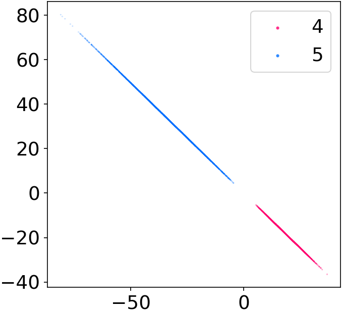
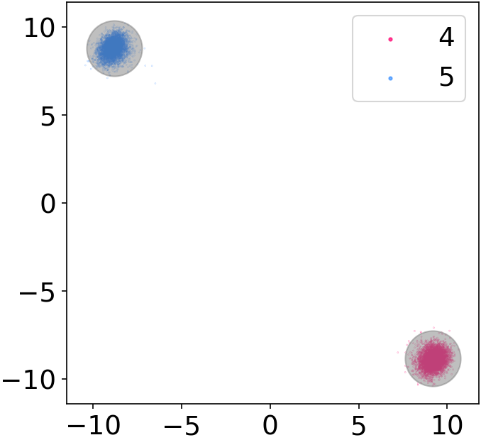
Open set

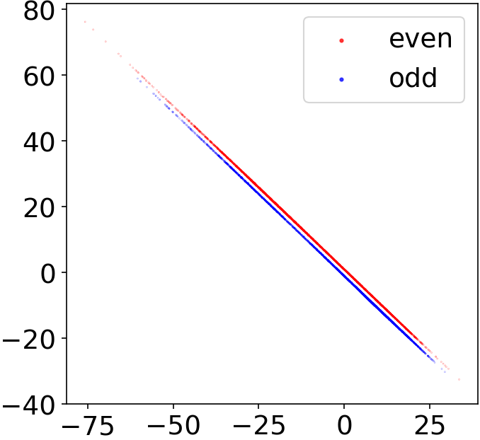
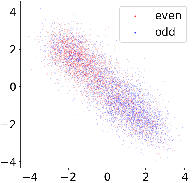
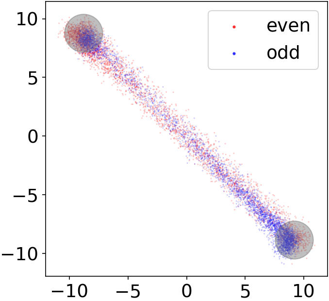
Figure 6: Latent space representation for MNIST. On the first row, we report the representations for 4 and 5 as fitted by CBNM, VAE and GlanceNet, respectively. On the second row, we display the scattering plot for points only belonging to the open set. For CBNM, we separated even and odd instances by $\Delta y=2$, since their representations strongly overlap. All plots comprise only the $z_{4},z_{5}$ axes.

D.1 Qualitative results

In Fig. 6, we show the latent space representations for different models on the MNIST leakage test, for both closed-set and open-set data points. To illustrate the contribution of our mixture prior, in addition to the CBNM and GlanceNet models, we also considered a simpler supervised VAE model. This model has the same encoder, decoder, and classifier as the GlanceNet, but uses a regular Gaussian prior. We found that this model achieved a similar level of leakage to CG-VAE. We display in Fig. 7 the reconstruction of a few random examples output by GlanceNet: the reconstructions of all instances belonging to the open-set greatly deviate from the original.

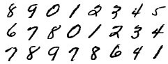
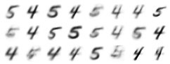
Figure 7: MNIST reconstruction with GlanceNet. On the left we reported the original digits, whereas on the right the reconstruction with the learned decoder. All images have been inverted in the black and white scale.

Appendix E Concept Leakage on dSprites

In this section, we report additional material for the dSprites concept leakage experiment. This experiment resembles the previous one on MNIST:

1. At training time, a CBM learns the representations of shape, size and rotation by receiving supervision on all possible variations of these factors. On the other hand, no variation of factors pos$\_$x and pos$\_$y are observed, in the sense that the position of the training sprites is fixed to the center of the image. We fit the CBNM and the GlanceNet with 5 latent factors to learn the representations. Again, no downstream classification task appears at this stage.

2. At test time, the encoder is kept fixed for different variations varying of the factors pos$\_$x and pos$\_$y are observed. The downstream task in this phase amounts to recognizing whether a sprite lies in top-right or in the bottom-left corner of the image.

In this experiment, concept leakage occurs if the accuracy on the downstream task is above the $50\%$.

Figure 8: Concept space representation of GlanceNet for dSprites. On the left, we show the projections on the one-hot encoded shape subspace, whereas on the right we project on the {size, rotation} subspace. We include the representations for training points, positive and negative ones.

E.1 Qualitative results

We also include qualitative results for GlanceNet and on dSprites for closed set and open set data points. In Fig. 8 we display the projections of train and test points on the two different latent subspaces (see caption). In both of them, positives and negatives representations are well separated from each other, implying substantia leakage. We also evaluated the reconstruction quality during training and testing and reported some of them in Fig. 9. Notably, almost all points are recognized to be open set instances thanks to the reconstruction threshold.

Closed set
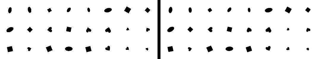
Open set

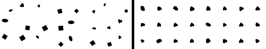
Figure 9: Reconstruction for dSprites on train and test with GlanceNet. On the upper panel, we report the reconstructions of the sprites belonging to the closed set. On the lower one, the reconstructions of the open set points. Like MNIST, all images have been inverted in the black and white scale.

Appendix F Additional results for GlanceNets and CBNMs in CelebA

In this section, we discuss additional results for CBNMs vs. GlanceNets on the CelebA dataset. We first report the accuracy of the learned concepts on the supervised latent factors for both CBNMs and GlanceNets in CelebA. Then, we examine two variants of GlanceNets varying the dimension of the unsupervised factors in the latent space: a $\beta$-VAE with 20 latent factors and a $\beta$-TCVAE with 40 latent factors, [39]. This variant includes an additional loss term given by the Total Correlation (TC) of the model posterior $q_{\phi}(\bm{\mathrm{z}})=\mathbb{E}_{p_{\mathcal{D}}(\bm{\mathrm{x}})}[q_{\phi}(\bm{\mathrm{z}}|\bm{\mathrm{x}})]$:

$$(\beta-1)\cdot\mathsf{KL}\big{(}q_{\phi}(\bm{\mathrm{z}})||\prod_{i=1}^{k}q_{\phi}(z_{i})\big{)}$$ (10)

where $\beta$ denotes the strength hyper-parameter. Both the $\beta$-VAE and the $\beta$-TCVAE receive supervision only on the 10 generative factors that are fitted in the CBNM. A the end of the section, we report traversals for the models with $40$ latent factors.

F.1 Concepts Accuracy

We report the concepts accuracy for both CBNMs and GlanceNets in Fig. 10, with 10 latent dimensions and the TCVAE variant. The difference in concept accuracy between GlanceNet (both variants) and CBNMs is negligible, with GlanceNets showing slightly higher variance when the percentage of concepts supervision is very small. This highlights how, in terms of concept accuracy, the two classes of models are essentially indistinguishable, even though they are in terms of alignment.

CBNMS $vs$ GlanceNets (10)	CBNMS $vs$ GlanceNets (40)

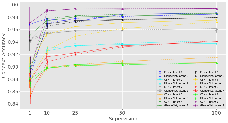
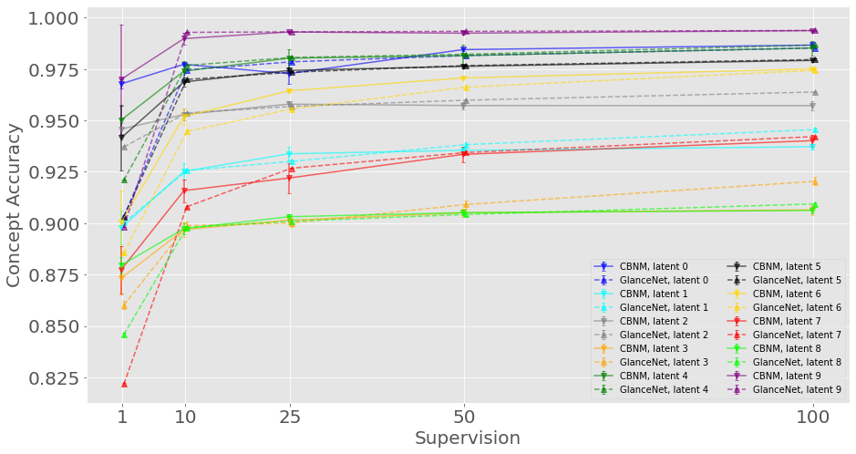
Figure 10: Concepts accuracy for CBNMs $vs$ GlanceNets. Different colors refer to the distinct attributes for which supervision is provided. The solid line is reserved to CBNMs, whether GlanceNets are displayed with a dotted line. On the left, CBNMs vs GlanceNets with a latent space of dimension 10. On the right, CBNMs vs GlanceNets with TCVAE variant and a latent space of 40.

F.2 Performances upon variations of the latent space dimension

Here, we show the behavior of the metrics upon increasing the dimension of the latent space. The first variant of GlanceNets, based on $\beta$-VAE, was fitted with $\beta\approx 1$, with a latent space of dimension 20. The second variant is a TCVAE, trained with a weight of the total correlation $\beta=10$ for all concepts supervisions, exception made for the $100$% run, where we found better results with $\beta=0.5$. We measured alignment and explicitness for both variants of GlanceNets by restricting on only those 10 latent factors where supervision were provided. This is in line with the notion of alignment, since we are interested in measuring the interpretability of the model, not the disentanglment among different components.

In Fig. 11 we report the results obtained, including the original variant with 10 latent dimensions. For the $\beta$-VAE (20) and TCVAE (40) we can see the improvement provided by extending the latent space. The latter achieves particular high values of alignment.

	Accuracy	Alignment	Explicitness
$\beta$-VAE (10)
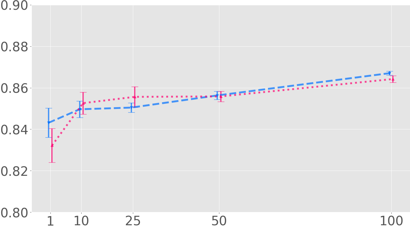
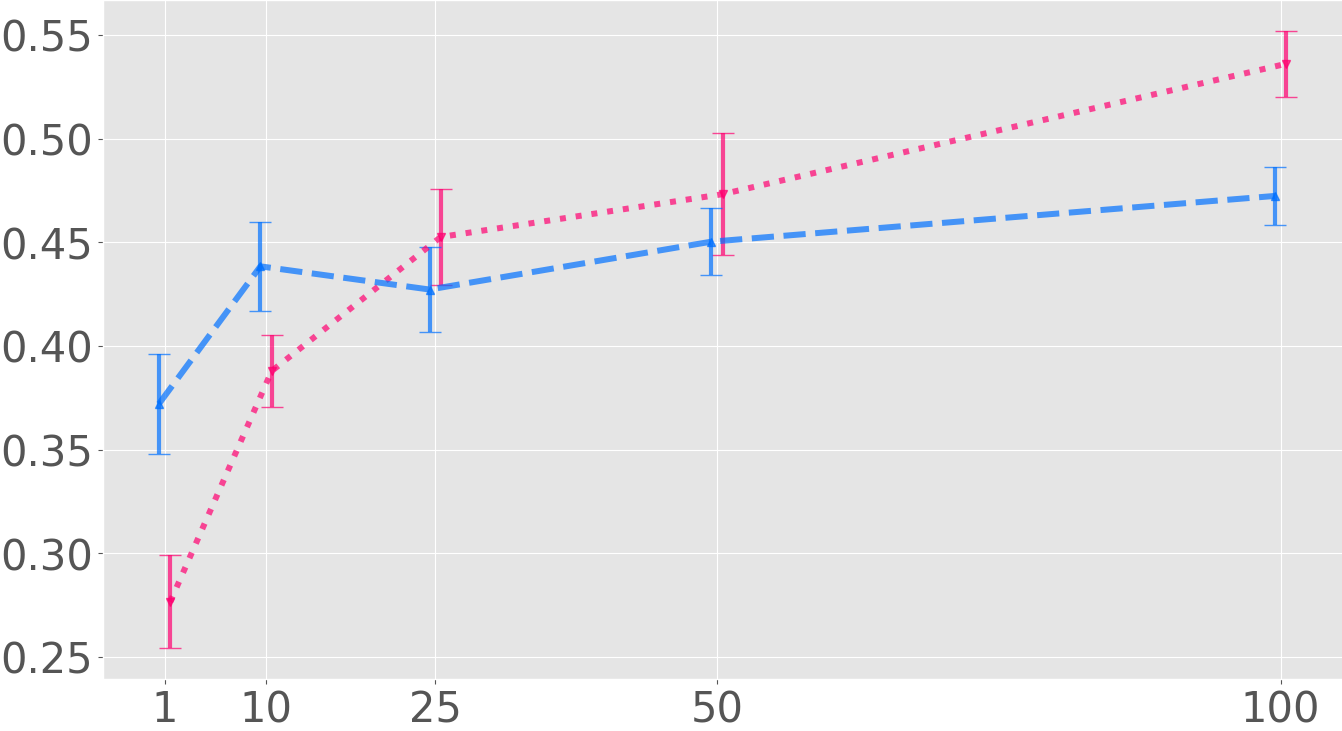
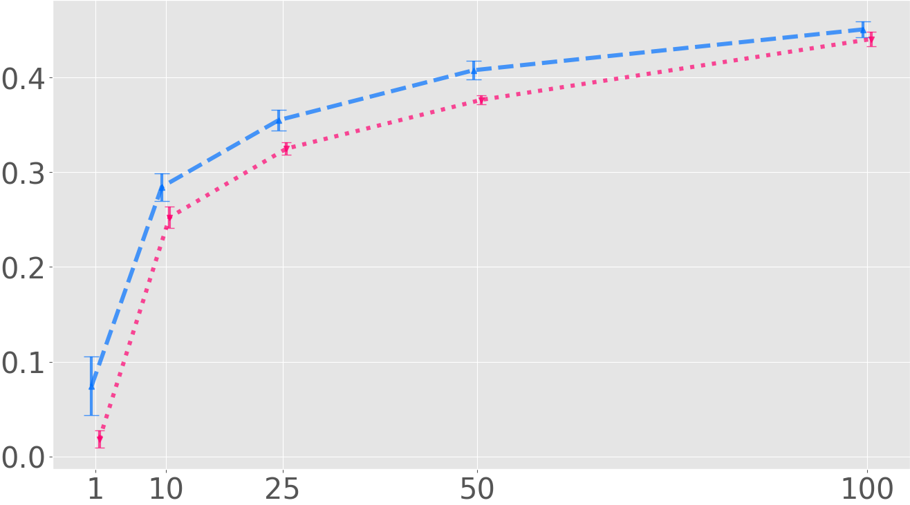
$\beta$-VAE (20)
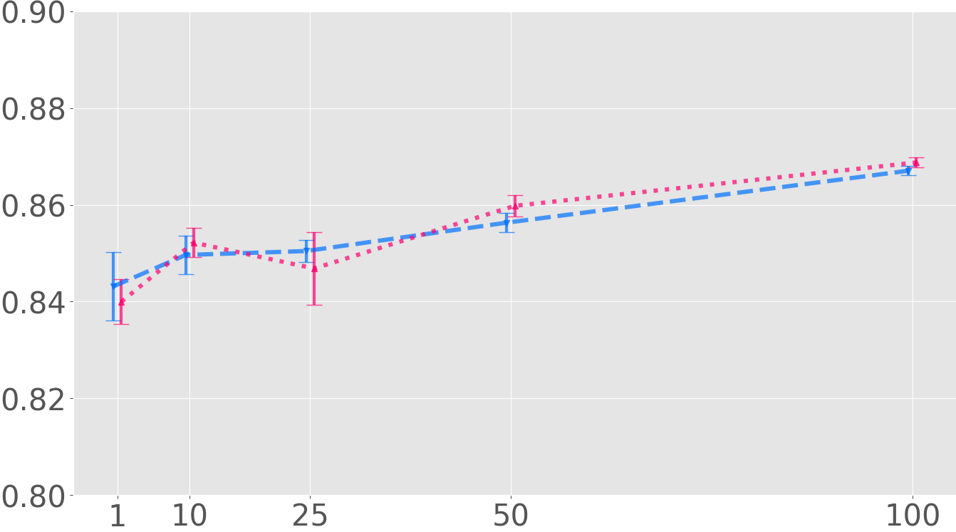
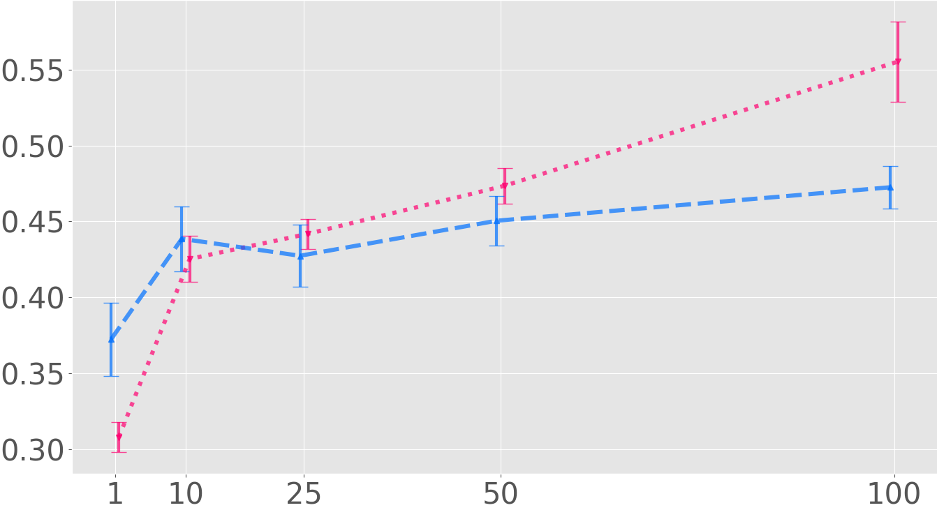
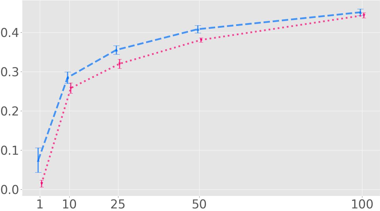
TCVAE (40)

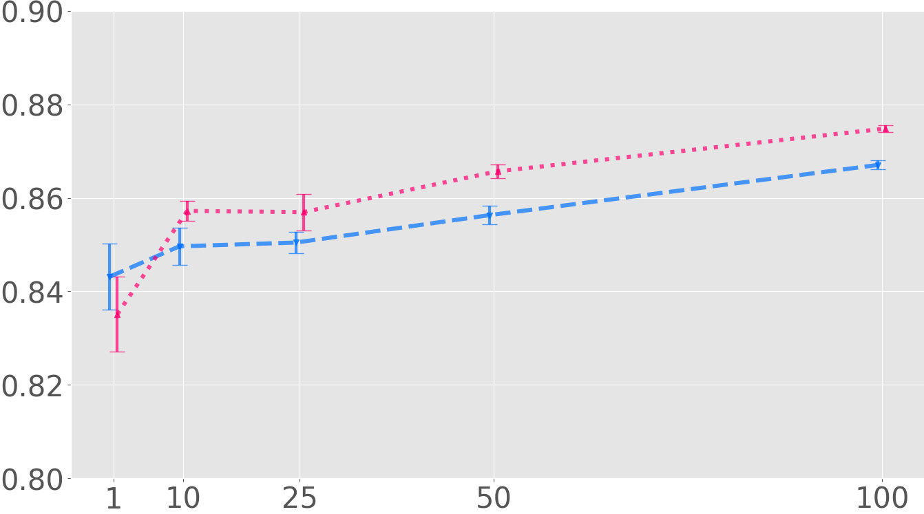
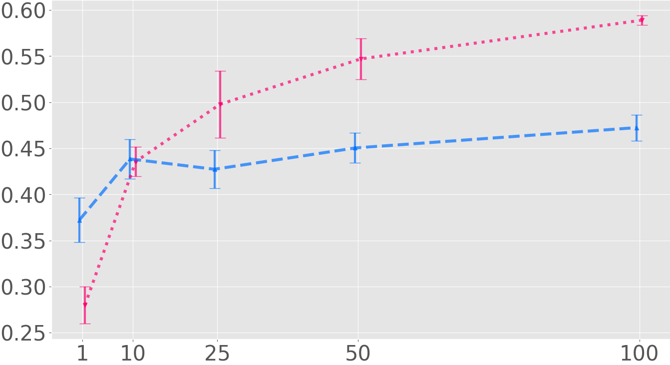
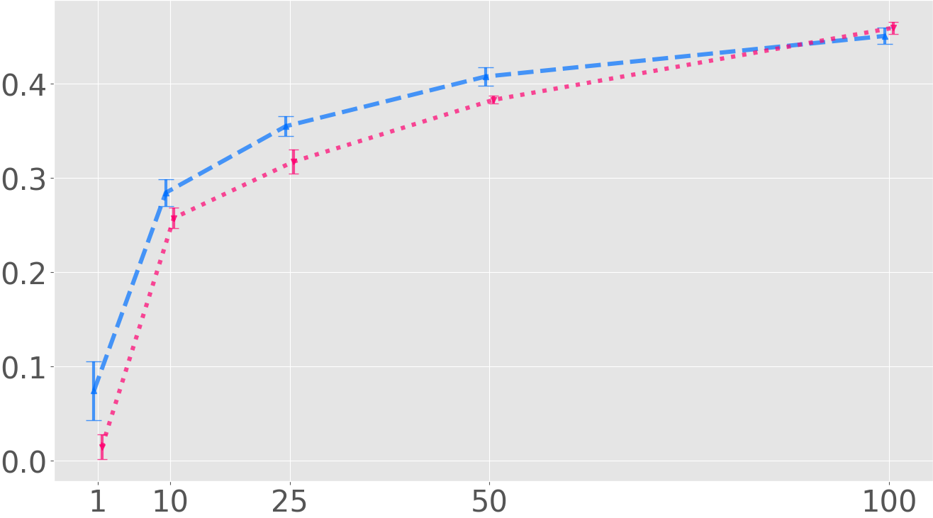
Figure 11: Accuracy, Alignment and Explicitness metrics for CBNMs $vs$ GlanceNets. For each row we vary the comparison with variants of GlanceNets: $\beta$-VAE (10) refers to the model we reported in the main text, $\beta$-VAE (20) is a variant with 20 latent dimensions, and TCVAE (40) is the model based on a TCVAE with 40 latent dimensions.

F.3 Latent traversals

We finally report in the traversals for some of the supervised attributes, obtained by the GlanceNet TCVAE with full supervision on the concepts. We excluded the traversals of the attributes hat and bald since the generator failed to reproduce them faithfully. The others are well captured by the model, as we reported in Fig. 12.

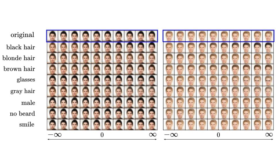
Figure 12: Latent traversals on two test images. In each row, we report the result of changing a single latent factor $Z_{i}$ (from $-5$ to $+5$) while keeping fixed the others.