Observations of the Very Young Type Ia Supernova 2019np with Early-excess Emission

Abstract

Early-time radiative signals from type Ia supernovae (SNe Ia) can provide important constraints on the explosion mechanism and the progenitor system. We present observations and analysis of SN 2019np, a nearby SN Ia discovered within 1-2 days after the explosion. Follow-up observations were conducted in optical, ultraviolet, and near-infrared bands, covering the phases from $\sim-$16.7 days to $\sim$+367.8 days relative to its $B-$band peak luminosity. The photometric and spectral evolutions of SN 2019np resembles the average behavior of normal SNe Ia. The absolute $B$-band peak magnitude and the post-peak decline rate are $M_{\rm max}(B)=$$-19.52\pm 0.47$ mag and $\Delta m_{\rm 15}(B)$ =$1.04\pm 0.04$ mag, respectively. No Hydrogen line has been detected in the near-infrared and nebular-phase spectra of SN 2019np. Assuming that the ⁵⁶Ni powering the light curve is centrally located, we find that the bolometric light curve of SN 2019np shows a flux excess up to 5.0% in the early phase compared to the radiative diffusion model. Such an extra radiation perhaps suggests the presence of an additional energy source beyond the radioactive decay of central nickel. Comparing the observed color evolution with that predicted by different models such as interactions of SN ejecta with circumstellar matter (CSM)/companion star, a double-detonation explosion from a sub-Chandrasekhar mass white dwarf (WD), and surface ⁵⁶Ni mixing, the latter one is favored.

1 Introduction

Since the late twentieth century, the studies of Type Ia supernovae (SNe Ia) have led to the discovery of the accelerating universe (Riess et al., 1998; Perlmutter et al., 1999; Riess et al., 2016, 2018, 2021). Nowadays, SNe Ia are widely used as standardizable candles in observational cosmology (Riess et al., 1996; Wang et al., 2005; Guy et al., 2005; Howell et al., 2006; Howell, 2011; Burns et al., 2018). However, the exact formation channel and explosion physics of SNe Ia are still unknown (Wang & Han, 2012; Wang et al., 2013a; Maoz et al., 2014; Jha et al., 2019).

Three popular scenarios for the explosion of SNe Ia are: 1) The ‘single-degenerate’ (SD) channel, in which a carbon–oxygen (CO) WD accretes matter from a nondegenerate companion such as a main-sequence star, a giant, or a He star. A thermonuclear explosion process is expected to occur when the progenitor CO WD reaches the critical Chandrasekhar mass of $M_{\rm Ch}\sim 1.4M_{\odot}$ (Whelan & Iben, 1973; Nomoto et al., 1997; Podsiadlowski et al., 2008; Wang et al., 2009a); 2) The ‘double-degenerate’ (DD) channel, in which the explosions of SNe Ia are triggered by the compressional heat generated by the dynamical merging process of two CO WDs (Webbink, 1984; Iben & Tutukov, 1984; Benz et al., 1990; Pakmor et al., 2012); 3) The direct head-on collision of two WDs in triple systems (Kushnir et al., 2013); however, the rate of head-on collisions of WDs in triple systems has been suggested too low to account for the majority of SNe Ia explosions (Toonen et al., 2018). In the SD channel, an extended CSM prorfile is expected to form around the progenitor system during its evolution towards a SN Ia explosion. Although the signature of CSM has been revealed for some SNe Ia via high-resolution spectroscopy (Hamuy et al., 2003; Aldering et al., 2006; Patat et al., 2007; Sternberg et al., 2011; Dilday et al., 2012; Maguire et al., 2013; Silverman et al., 2013), the lack of narrow H emission lines in the late-time spectra still challenges the SD model (Mattila et al., 2005; Leonard, 2007; Shappee et al., 2013; Maguire et al., 2016; Tucker et al., 2020). Additionally, searches for pre-explosion or surviving companions of the progenitor through deep images (Li et al., 2011; González Hernández et al., 2012; Schaefer & Pagnotta, 2012) have firmly excluded the presence of giant and subgiant companions.

On the other hand, detection of the first light after a SN explosion can also provide important constraints on progenitors of SNe Ia (Kasen, 2010). In a SD progenitor system, the SN ejecta could run into the nondegenerate companion or surrounding CSM. Then an excess of ultraviolet (UV)/optical emission could be generated and become detectable within the first few days for the interaction between SN ejecta and a companion star or within a few hours for the interaction between SN ejecta and ambient CSM. For the former case, the flux excess can last for a few days, depending on the size of the companion, the progenitor-companion separation, the ejecta velocity, and the viewing angle. During the Kepler mission (Haas et al., 2010), a few SNe were detected in the Kepler fields, including two spectroscopically confirmed SNe Ia and three possible ones. There is no signature of ejecta interaction with a stellar companion for the latter three (KSN 2012a, KSN 2011b and KSN 2011c) (Olling et al., 2015) and SN 2018agk (Wang et al., 2021). Blue excess flux was detected in the early-time light curve of SN 2018oh, however, the explanations are not converged (Dimitriadis et al., 2019; Shappee et al., 2019; Li et al., 2019). For example, both the deep mixing carbon feature and nondetection of hydrogen in the nebular-phase spectrum of SN 2018oh do not favour a SD scenario for its origin (Li et al., 2019; Tucker et al., 2019). A similar “blue bump” feature was also detected in the nearby SN 2017cbv (Hosseinzadeh et al., 2017), but analysis of the nebular-phase spectroscopy argues against a nondegenerate H- or He-rich companion as its progenitor (Sand et al., 2018). For the latest case, however, the extra emission in the early time usually lasts for a few hours, depending on the density and distance of the CSM. In a recent study, SN 2020hvf is reported to have such an early-time excess emission (Jiang et al., 2021).

Besides interaction with a companion star or CSM disk, the early excess emission may also be produced by other mechanisms, e.g., radioactive decay of ⁵⁶Ni near the surface of the exploding WD (Piro & Nakar, 2013; Magee et al., 2020). Mixing of ⁵⁶Ni into the outer layers would result in bluer and steeper rising light curves (Piro & Morozova, 2016) and this mechanism works for both SD and DD progenitors. Magee et al. (2020) shows that the observed diversity in light curves of SNe Ia can be reproduced by varying the distribution of ⁵⁶Ni. Another explosion model that can produce such ⁵⁶Ni distribution is the double-detonation explosion of a sub-Chandrasekhar mass WD, where the initial detonation of the outer-layer He would produce a certain amount of nickel near the surface and it sends a shockwave to the C/O core to trigger the second detonation (Woosley & Weaver, 1994; Wang et al., 2013b; Noebauer et al., 2017), thus leading to a wide range of absolute magnitudes and colors. However, in order to match the observed peak brightness of SNe Ia, this model requires that the number of iron-group elements (IGEs) synthesized during He shell detonation is very small. The radioactive decay of the surface material would produce photons and they diffuse out of the ejecta rapidly, which results in a flux excess in the first few days after explosion.

The detection of the very young thermonuclear SN 2019np provides us a rare opportunity to examine the first-light evolution of a SN Ia. In this paper, we present extensive follow-up observations of SN 2019np within the UV to NIR wavelength ranges. We also analyze its photometric and spectroscopic behaviours and compare the observational properties of SN 2019np with those of other well-studied SNe Ia. Observations and data reduction are outlined in Section 2, the light/color curves are described in Section 3, and the spectroscopic behavior of SN 2019np and its temporal evolution are presented in Section 4. We discuss the properties of SN 2019np and its explosion parameters in Section 5. The conclusions are given in Section 6.

2 observations

SN 2019np was discovered on 2019 Jan. 9.67 (UT) by K. Itagaki in NGC 3254 which is an Sbc-type spiral galaxy (see Figure 1) with a redshift of only 0.00452. The classification spectrum obtained $\sim$one day after the discovery suggests that SN 2019np was a very young, normal SN Ia, at $\sim$15 days before the maximum luminosity (Wu et al., 2019; Kilpatrick & Foley, 2019).

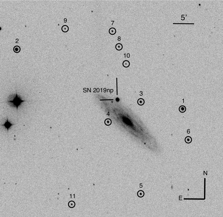
Figure 1: Image of SN 2019np in NGC 3254, taken with Tsinghua-NAOC 0.8 m telescope. Reference stars are marked with black circles and listed in Table 2. North is up and east is left.

2.1 Photometry

Photometric observations were obtained through various facilities including: (1) the 0.8 m Tsinghua-NAOC Telescope (TNT) in China (Huang et al., 2012); (2) the Lijiang 2.4 m Telescope (LJT) at Yunnan Observatory; (3) the 0.8 m Joan Oró Telescope+MEIA3 at Montsec Astronomical Observatory (Spain); (4) the 0.67/0.92 m Schmidt Telescope at Mount Ekar Observatory (Italy); (5) the 1.8 m Copernico Telescope+AFOSC at Mount Ekar Observatory (Italy); (6) the 2.6 m Nordic Optical Telescope (NOT)+ALFOSC at the Roque de Los Muchachos Observatory (Spain); (7) the 0.6 m reflector telescope+BITRAN-CCD at Itagaki Astronomical Observatory (Japan). All images were pre-processed, including bias subtraction, flat-field correction, and cosmic-ray rejection with the standard IRAF packages. We use the pipeline Zuruphot developed for automatic photometry on TNT (Mo et al. in prep) to perform point-spread-function (PSF) photometry for both SN 2019np and local reference stars.

The instrumental magnitudes were then converted to the Johnsons $BV$ (Johnson et al., 1966) and Sloan Digital Sky Survey (SDSS) $gri$-band photometry (Fukugita et al., 1996), based on the magnitude of 10 relatively bright local comparison stars from the SDSS Data Release 9 catalog. SN 2019np was also observed by the Ultra-violet/Optical Telescope (UVOT; Gehrels et al., 2004; Roming et al., 2005) on the Neil Gehrels Swift Observatory (Gehrels et al., 2004) in three UV ($uvw2$, $uvm2$, $uvw1$) and three optical filters ($u$, $b$, $v$). Photometry was extracted using the HEASOFT with the latest Swift calibration database . The final Optical and UV magnitudes are reported in Table 6 and LABEL:swift, respectively.

2.2 Spectroscopy

Optical spectra of SN 2019np were obtained with the Lijiang 2.4 m telescope (LJT+YFOSC); Xinglong 2.16 m telescope (XLT+BFOSC) (Zhang et al., 2016a); the 1.8 m Copernico Telescope+AFOSC at the Mount Ekar Observatory (Italy); the Alhambra Faint Object Spectrograph Camera (ALFOSC) on the 2.56 m Nordic Optical Telescope (NOT); the 10.4 m Gran Telescopio CANARIAS (GTC)+OSIRIS at the Roque de Los Muchachos Observatory (Spain); and the 2.0 m Faulkes Telescope North (FTN)+FLOYDS at Haleakala Observatory (USA), spanning from $-16.7$ to 367.8 days (d) relative to the $B-$band maximum light. A journal of spectroscopic observations of SN 2019np is presented in Table 4. We reduced all the spectra using the standard IRAF routine. Flux calibration of the spectra was performed with spectrophotometric standard stars taken on the same nights. We correct the atmospheric extinction using the extinction curves of local observatories. The telluric correction was derived from the spectrophotometric standard star spectral observations and applied to the SN spectra.

Two near-infrared (NIR) spectra of SN 2019np were obtained using the Folded port InfraRed Echellette (FIRE, Simcoe et al., 2013) spectrograph mounted on the 6.5-m Magellan Baade telescope at Las Campanas Observatory, Chile. The spectra cover a wavelength range of 0.8-2.5 $\mu m$ with the high-throughput prism mode coupled to a 0.”6 slit. For telluric correction, we observed an A0V star close in time and at approximately similar air mass to SN 2019np (Hsiao et al., 2015, 2019). The spectra were reduced using the IDL pipeline firehose (Simcoe et al., 2013). We also present two NIR spectra obtained with the SpeX spectrograph (Rayner et al., 2003) mounted on the NASA Infrared Telescope Facility (IRTF) in Hawaii. A short cross-dispersed mode has been used and a 0.”5 slit was placed on the target, providing a wavelength coverage of 0.8-2.5 $\mu m$. The SpeX data were reduced using the IDL code Spextool (Cushing et al., 2004). A journal of spectroscopic observations of SN 2019np is presented in Table 5.

3 Photometry

3.1 Optical and UV Light Curves

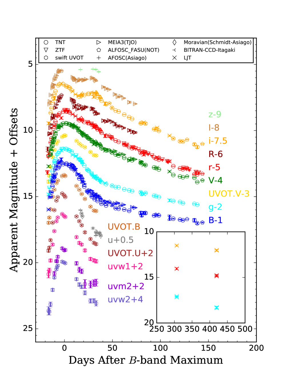
Figure 2: Optical and UV light curves of SN 2019np. Different colors represent different bands, including the Swift uvw2, uvm2, uvw1, UVOT U, u, UVOT B, B, g, UVOT V, V, r, R, i, I and z. The insert panel shows the late-time light curves.

Figure 2 shows the UV and optical light curves of SN 2019np sampled during the period from -16.5 to +32.8 days and that from -17.7 to 419.5 days relative to the $B-$band maximum light, respectively. Similar to other normal SNe Ia, the light curves of SN 2019np show shoulders in the $R/r$ bands. Secondary peaks can be identified in $I/i$-band light curves, for which the first peak appears about 2 days earlier than the $B-$band peak.

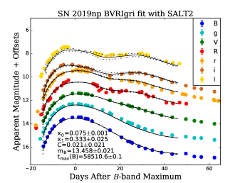
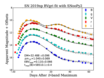
Figure 3: Best-fit light-curve models from SALT2 (left panel) and SNooPy2 (right panel). The light curves of different bands have been shifted vertically for better display. The dashed lines represent the 1-$\sigma$ uncertainty of the light-curve templates. The parameter $x_{0}$ represents the normalization of the SED sequence, $x_{1}$ is the light curve shape parameter and C stands for the color. $m_{\textup{B}}$ and $t_{\textup{max}}$(B) denote the maximum magnitude of the $B-$band and the corresponding time. DM is the distance modulus.

We applied high-order polynomial fits to the light curves of SN 2019np around the maximum light and estimated that it reached a $B-$band peak magnitude of $13.55\pm 0.02$ mag on MJD $58510.2\pm 0.8$ and a $V-$band peak magnitude of 13.62$\pm 0.15$ mag on $58512.5\pm 0.7$, respectively. The post-peak magnitude decline in 15 days from the $B-$band peak, $\Delta m_{\rm 15}(B)$ (Phillips et al., 1999), as determined using the light-curve fitting tools SALT2 (Guy et al., 2010) and SuperNovae in object-oriented Python (SNooPY2, Burns et al., 2011), is estimated as $1.038\pm 0.004$ and $1.040\pm 0.069$ mag, respectively. The best-fit light-curve models and the associated parameters are presented in Figure 3.

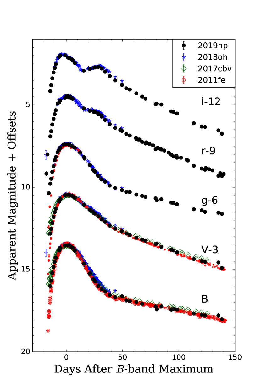
Figure 4: Comparison of the optical light curves of SN 2019np with other well-observed SNe Ia with similar decline rates. The light curves of the comparison SNe Ia have been normalized to match the peaks of SN 2019np.

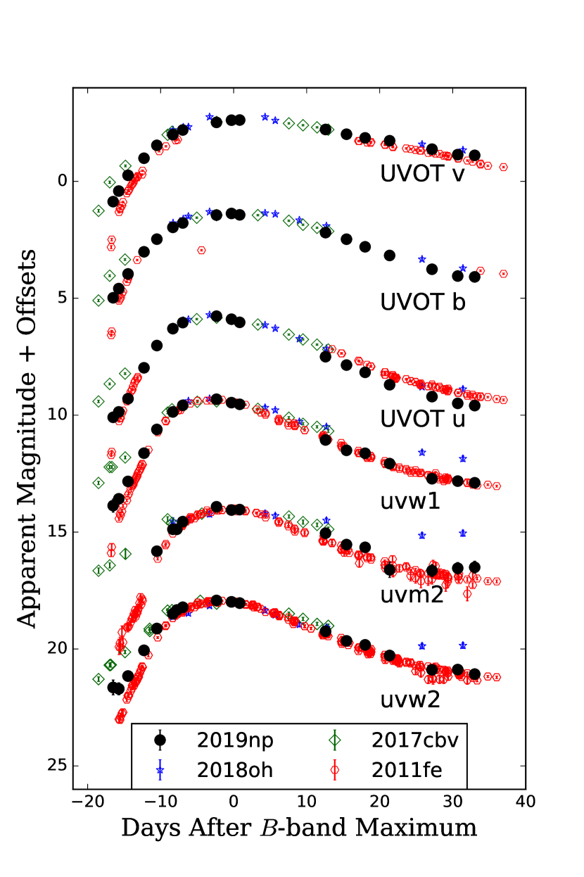
Figure 5: The UV light curves of SN 2019np compared with other well-sampled SNe Ia with similar decline rates. The light curves of the comparison SNe Ia are normalized to match the peaks SN 2019np.

In Figures 4 and 5 we compare the optical and UV-band light curves, respectively, between SN 2019np and several other well-observed normal SNe Ia with similar values of $\Delta m_{\rm 15}$. The comparison sample include SN 2018oh (Li et al., 2019), SN 2017cbv (Hosseinzadeh et al., 2017; Wang et al., 2020) and SN 2011fe (Silverman et al., 2012; Tsvetkov et al., 2013; Zhang et al., 2016b; Stahl et al., 2019). The optical light curves of SN 2019np exhibit high similarities to those of SN 2017cbv ($\Delta m_{\rm 15}(B)=1.06\pm 0.3$ mag). Closer inspection of the UV light curves reveals that SN 2019np shows exceptionally blue UV radiation in the very early phase, which is also similar to SN 2017cbv.

3.2 Reddening

The Galactic extinction toward SN 2019np is estimated as $A_{V}({\rm Gal})=0.055\,$mag according to the dust map derived by Schlafly & Finkbeiner (2011). Adopting the Cardelli et al. (1989) extinction law with a total-to-selective extinction ratio of 3.1, the reddening due to Milky Way is $E(B-V)_{\rm Gal}=0.018$ mag. This is consistent with the weak Na iD absorption due to the Milky Way.

Furthermore, we examined the absorption of the interstellar Na iD doublet (5895.92, 5889.95 Å) due to the host galaxy and derived an equivalent width (EW) of 0.68Å for SN 2019np from its near-maximum-light spectra. This corresponds to a host-galaxy reddening of 0.10$\pm$0.02 mag according to the empirical relation proposed by Poznanski et al. (2012) (i.e., $\log_{10}(E(B-V))=1.17\times\rm{EW}(\rm{D_{1}}+\rm{D_{2}})-1.85$), and a similar result with larger dispersion has been updated by Phillips et al. (2013). We also employed SNooPy2 (Burns et al., 2011) to fit the multi-band light curves of SN 2019np to determine the host-galaxy reddening, which gives $E(B-V)_{\rm host}=0.110\pm 0.066\,$mag. The best-fit results are also shown in Figure 3. We averaged the reddening estimated by the above methods and adopted $E(B-V)_{\rm host}$=$0.10\pm 0.04$ mag as the final value. Moreover, an extinction law with $R_{V}=3.1$ (Cardelli et al., 1989) is adopted throughout this paper.

After correcting for the reddening due to the Milky Way and host galaxy, the $B-V$ color of SN 2019np is found to be $-0.06\pm 0.03$ mag around the $B-$band maximum light, in consistent with that of a normal SN Ia (see, e.g., Wang et al. 2009b).

3.3 Color Curves

In Figure 6, we compare the color evolution of SN 2019np with that of some well-observed SNe Ia with similar $\Delta m_{\rm 15}(B)$. At early times, SN 2019np showed blue colors similar to SN 2011fe, SN 2017cbv and SN 2018oh. After that, the $B-V$ and $g-r$ color curves evolve bluewards and reach the minimum value at about 10 days prior to the $B$-band maximum. Then they evolve redwards again and reach the red peak at t$\sim 30$ d; and they gradually become blue after the red peak.

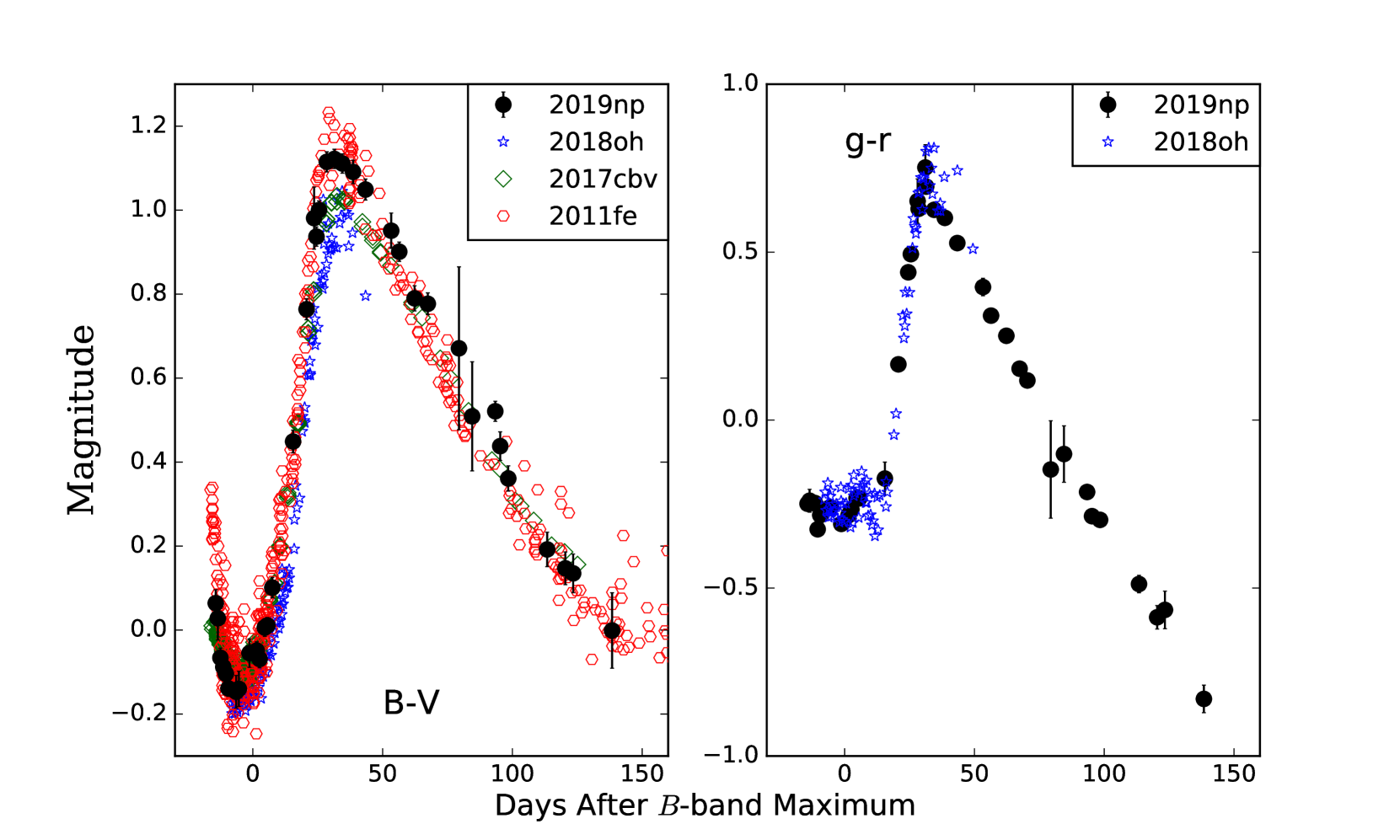
Figure 6: Reddening-corrected $B-V$ (left panel) and $g-r$ (right panel) color curves of SN 2019np, compared with those of SNe 2018oh, 2017cbv and 2011fe.

4 Spectroscopy

4.1 Temporal Evolution of the Optical Spectra

Figure 7 shows the spectral evolution of SN 2019np in the optical wavelength range. The spectral evolution follows that of normal SNe Ia. For example, within the first weeks after the explosion, the spectra of SN 2019np are characterized by prominent absorption lines of intermediate-mass elements (IMEs) and ionized IGEs. By the time SN 2019np stepped into the early nebular phase, absorption features of IGEs start to dominate the spectra.

Figure 8 shows the spectral comparison between SN 2019np and some well-observed normal SNe Ia with similar decline rates at different epochs. The earliest spectrum obtained at t$\sim-16.6$ d is dominated by prominent absorption lines of IMEs and IGEs. Note that weak absorption features of C ii $\lambda$6580 and C ii $\lambda$7234 can clearly be identified in its earliest spectra. The absorption feature near 4300 Å could be due to the Mg ii $\lambda$4481 line blended with the Fe ii $\lambda$4404 line, while the blended lines of Fe iii $\lambda$5129, Fe ii $\lambda\lambda\lambda$4924,5018,5169 and Si ii $\lambda$5051 are responsible for the broad absorption near 4800 Å. The Ca ii H&K and Ca ii NIR triplet contribute to the prominent absorption features near 3700 Å and 8000 Å, respectively. In the spectrum at t$\sim-10.5$ d spectrum, the “W”-shaped S ii absorption features near 5400 Å and the Si ii $\lambda$5972 feature near 5800 Å start to show up in the spectra and gain their strengths. By this phase, the C ii $\lambda$6580 absorption is still visible in SN 2019np, SN 2011fe, and SN 2018oh, but it disappears in SN 2012cg and SN 2013dy. Detached high velocity feature (HVF) can be clearly seen in Ca ii NIR triplet of SN 2019np, which is similar to the comparison SNe Ia. The spectra around the maximum light are characterized by the prominent absorption features of Ca ii H&K, S ii, Si ii $\lambda$6355 and Ca ii NIR triplet. Note that the C ii $\lambda$6580 absorption feature still seems visible in SN 2019np, SN 2011fe and SN 2018oh. The HVF of the Ca ii NIR triplet becomes weak while the photospheric component gain its strength. At t$\sim 1$ month, the characteristic Fe ii features within the wavelength range of $4600-5300$Å start to develop and dominate in the spectra. At this phase, the overall spectral features of SN 2019np and the comparison SNe Ia become quite similar. Spectroscopically, SN 2019np is found to be more similar to SN 2011fe.

Figure 9 shows the spectra taken at t$\sim$144 d and t$\sim$303 d after the maximum light, when forbidden lines of ionized IGEs such as Fe and Co dominate in the spectra. One can see that the late-time behaviour of SN 2019np also exhibits considerable similarities to that of SNe 2011fe, 2013dy, and 2018oh. Combining the spectra at t $\sim$144 d and $\sim$303 d, we notice that the [Fe III] feature at $\sim 4700$Å  [Co II] at $\sim 6000$Å  and [Fe II]/[Ni II] at $\sim 7200$Å tend to become relatively weak with time. From the t$\sim$303 d spectrum, we measured the velocity shift of forbidden emission lines of [Fe ii]$7155$Å and [Ni ii]$7378$Å as $1550\pm 140$ km s^-1, which is consistent with that of the comparison normal SNe Ia (i.e. SN 2011fe and SN 2018oh).

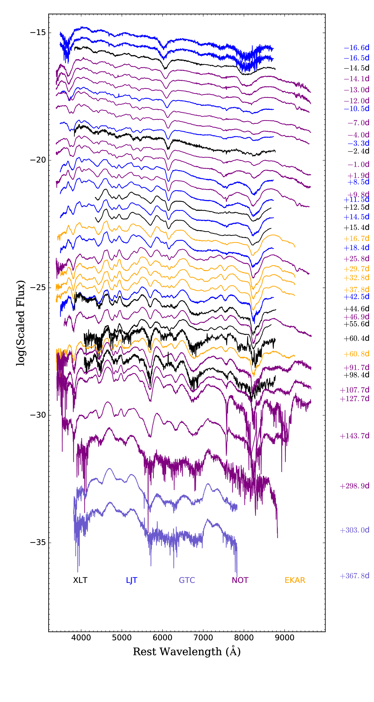
Figure 7: Optical spectral evolution of SN 2019np from $-16.6$ days to $+367.8$ days relative to the B-band maximum light. The spectra have been corrected for host-galaxy redshift (z = 0.00452) and reddening. The text on the right side of each spectrum denotes the phase in days since the $B$-band maximum light. Different colors of the spectra represent that they were taken with different spectroscopic instruments (i.e., XLT, LJT, GTC, NOT or EKAR), which are indicated at the bottom of the plot.

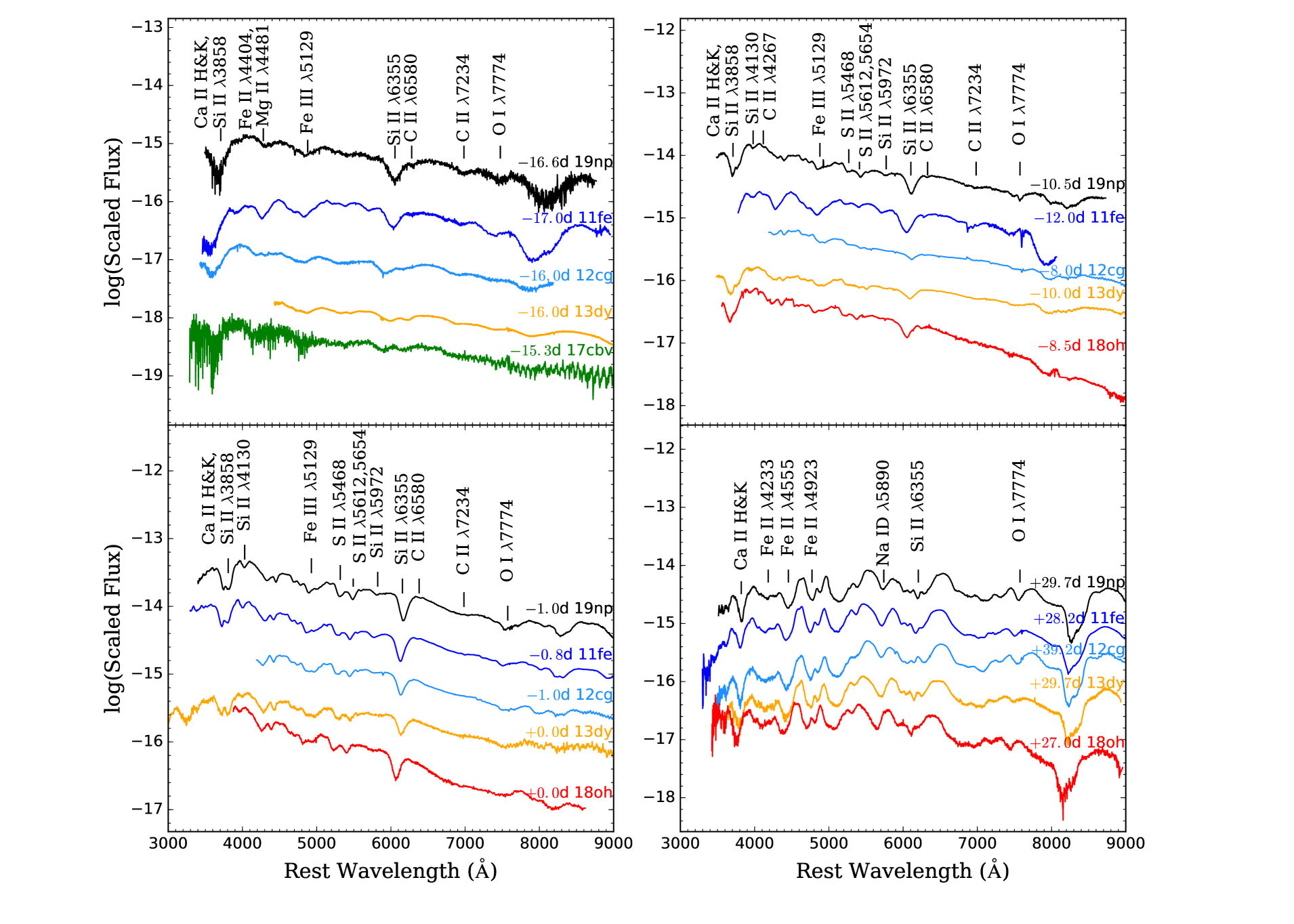
Figure 8: Spectral comparison between SN 2019np and some well-studied SNe Ia at several selected epochs (i.e., t$\sim-16.0$ days, $-10.0$ days, $0$ days, and $+30.0$ days). The comparison objects include SNe 2011fe (Mazzali et al., 2014; Zhang et al., 2016b), 2012cg (Marion et al., 2016), 2013dy (Zheng et al., 2013; Pan et al., 2015; Zhai et al., 2016), 2017cbv (Hosseinzadeh et al., 2017) and 2018oh (Li et al., 2019). All spectra have been corrected for reddening and the host-galaxy redshifts. For better display, all spectra were shifted arbitrarily along the vertical direction.

Figure 9: Nebular-phase spectra of SN 2019np obtained at t$\sim+144$ d (left panel) and $+303$ d (right panel) compared with the spectra of a few well-observed SNe Ia at similar phases, including SNe 2011fe (Silverman et al., 2012; Yaron & Gal-Yam, 2012), 2013dy (Zheng et al., 2013; Zhai et al., 2016) and 2018oh (Tucker et al., 2019). All spectra were corrected for host-galaxy redshifts. The yellow and red spectra have been smoothed by a Savitsky–Golay filter.

4.2 Ejecta Velocity

We measure the ejecta velocities of SN 2019np using the absorption minima of a series of spectral features including Si ii $\lambda$6355, S ii $\lambda$5468, C ii $\lambda$6580, Ca ii NIR triplet, and the result is shown in Figure 10. All velocities have been corrected to the restframe of the host galaxy based on its redshift. The photospheric velocity of Si ii $\lambda$6355 at t$\sim$-16.6 d is $\sim$16,100 km s^-1, which is higher compared to that measured from the C ii $\lambda$6580 velocity of $\sim$15,000 km s^-1.

The velocity of Si ii $\lambda$6355 is measured as 10,200 km s^-1 at the time of $B$-band maximum, which is comparable to the typical value (i.e., $\sim$10,500 km s^-1) of normal SNe Ia and can be clearly put into the normal velocity group according to the classification scheme proposed by Wang et al. (2009c). The velocity of Si ii $\lambda$6355 exhibits a similar evolution as that measured from the C ii $\lambda$6580 and S ii $\lambda$5468.

Basic photometric and spectroscopic parameters of SN 2019np are listed in Table 1. The velocity evolution of SN 2019np as derived from the Si ii $\lambda$6355 line is presented in Figure 11. The velocity evolution of SNe 2018oh, 2013dy, 2005cf (Wang et al., 2009b) and 2011fe are also shown for comparison. The velocity gradient of Si ii $\lambda$6355 measured 10 days past maximum is $\dot{v}_{\rm{Si}}$=$21\pm 5$ km s^-1 d^-1, indicating that SN 2019np belongs to the low-velocity gradient (LVG) subclass according to the classification scheme proposed by Benetti et al. (2005).

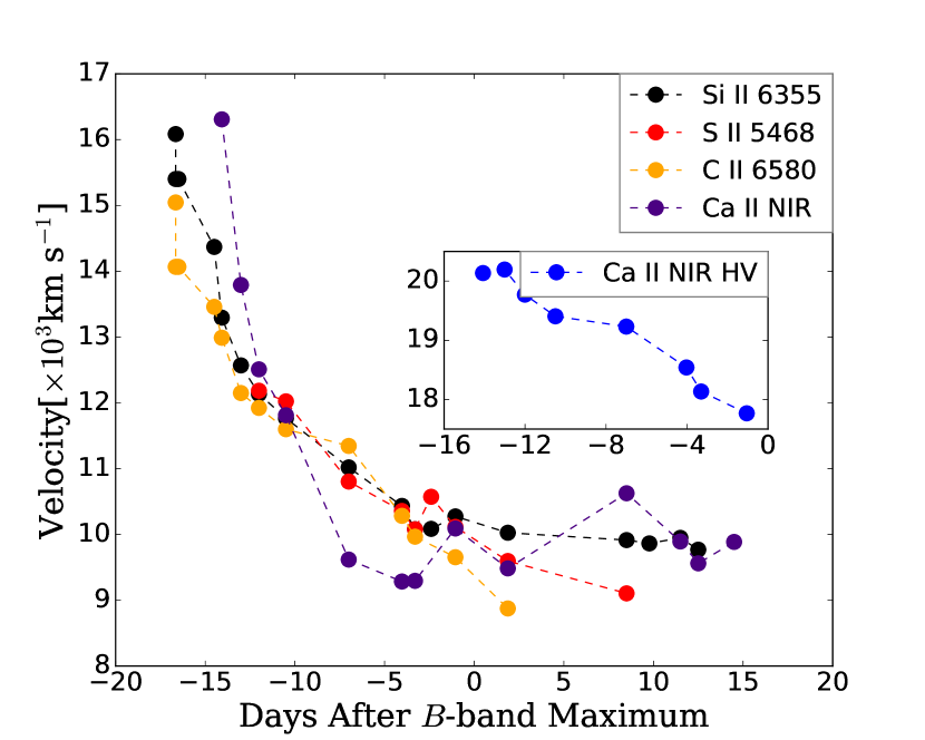
Figure 10: Evolution of the expansion velocity of SN 2019np as measured from the absorption minimum of Si ii $\lambda$6355, S ii $\lambda$5468, C ii $\lambda$6580 and Ca ii NIR triplet.

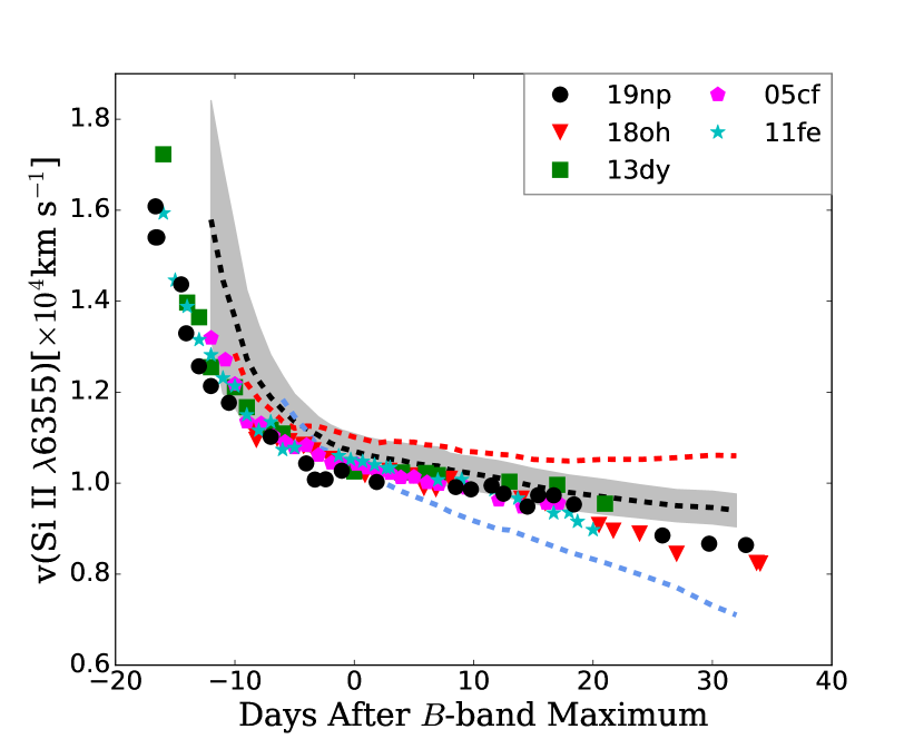
Figure 11: Velocity evolution of SN 2019np as measured from the absorption minimum of Si ii $\lambda$6355, compared to that of SNe 2018oh, 2013dy, 2005cf and 2011fe. Overplotted curves present the velocity evolution obtained for SN 1991T-like (red dashed), SN 1991bg-like (blue dotted), and normal (solid black) subclasses of SNe Ia (Wang et al., 2009c). The gray-shaded region indicates the 1-$\sigma$ standard deviation of the mean velocity of normal SNe Ia.

Table 1: Parameters of SN 2019np

Parameter	Value
Photometric
$B_{\rm max}$	$13.55\pm 0.02$ mag
$B_{\rm max}-V_{\rm max}$	$0.005\pm 0.007$ mag
$M_{\rm max}(B)$	$-19.52\pm 0.47$ mag
$E(B-V)_{\rm host}$	$0.10\pm 0.04$ mag
$\Delta m_{\rm 15}(B)$	$1.04\pm 0.04$ mag
$s_{BV}$	$0.98\pm 0.01$
$t_{\rm max}(B)$	$58510.2\pm 0.8$ d
$t_{0}$	$58494.09\pm 0.03$ d
$\tau_{\rm rise}$	$15.1\pm 0.8$ d
$L_{\rm bol}^{\rm max}$	$1.70\pm 0.63\times 10^{43}$ erg s-1
$M_{{}^{56}\rm Ni}$	$0.66\pm 0.05\,M_{\odot}$
$\mu$	$32.58\pm 0.45$ mag
Spectroscopic
$v\rm_{0}$(Si ii)	$10,200\pm 141$ km s-1
$\dot{v}$(Si ii)	$21\pm 5$ km s-1 d-1
$R$(Si ii)	$0.17\pm 0.01$

4.3 NIR Spectra

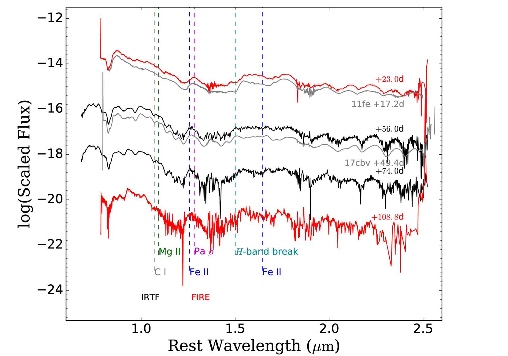
Figure 12: NIR spectra of SN 2019np from FIRE and IRTF, along with the comparable-phase spectra of SN 2011fe (Hsiao et al., 2013) and SN 2017cbv (Wang et al., 2020).

Figure 12 shows the NIR spectra of SN 2019np taken with IRTF and FIRE. We also compared the t$=+23.0$ d and $+56.0$ d spectra with SN 2011fe and SN 2017cbv.

The nondetection of the Pa$\beta$ feature indicates that the mass of hydrogen contained in companion star is less than 0.1 $M_{\sun}$ (Wang et al., 2020). The lack of hydrogen features in the nebular spectra is also in accord with a low hydrogen mass limit (Sand et al., 2018).

Moreover, the $H$-band break is observed around 1.5$\mu$m in the NIR spectra of SN 2019np, which is related to the dramatic shift in the amount of line blanketing from IGEs (Wheeler et al., 1998). Similar to other SNe Ia (Sand et al., 2018), a decrease in strength of the $H$-band break can be identified in SN 2019np during the phases from $t=+23.0$ to $+108.8$ d. Such a time evolution of the $H$-band break is related to the quantity of intermediate-mass elements, depending on different explosion scenarios, which can be further used to determine mass of ⁵⁶Ni (Hsiao et al., 2019; Ashall et al., 2019).

5 Discussion

5.1 Quasi-bolometric Light Curve

The distance of the host galaxy NGC 3254 is 32.80 $\pm$ 6.8 Mpc according to Tully-Fisher relation (Tully et al., 2016). Assuming $R_{V}=3.1$, the absolute magnitude of $B$-band peak is estimated as $M_{\rm{max}}(B)=$$-19.52\pm 0.47$ mag after correcting for the Galactic and host-galaxy extinctions. We derived the quasi-bolometric luminosity of SN 2019np based on Swift UV and optical photometry. Assuming that the NIR-band emission of SN 2019np has a similar contribution as in SN 2011fe (Zhang et al., 2016b), the quasi-bolometric light curve of SN 2019np is shown in Figure 13. The maximum-light luminosity is $L_{\rm peak}=$$1.70\pm 0.63\times 10^{43}$ erg s^-1, which is slightly larger than SN 2011fe ($L_{\rm peak}^{\rm 11fe}=1.13\times 10^{43}$ erg s^-1, Zhang et al. 2016b). We use the Minim Code (Chatzopoulos et al., 2013), based on the radiation diffusion model from Arnett (Arnett, 1982; Chatzopoulos et al., 2012; Li et al., 2019; Zeng et al., 2021), to estimate the nickel mass and other parameters. The relevant result is shown in Figure 14. The fitting parameters include first-light time $t_{0}=$$58494.09\pm 0.03$, the mass of the radioactive nickel $M_{\rm Ni}=$$0.66\pm 0.05\,M_{\odot}$, the light-curve timescale $t_{\rm lc}=$$11.19\pm 0.01$ days, and the gamma-ray leaking timescale $t_{\gamma}=$$37.42\pm 0.70$ days (Chatzopoulos et al., 2012). Then the inferred ejecta mass ($M_{\mathrm{ej}}$) and expansion velocity ($v_{\textup{exp}}$) can be calculated from $t_{\rm lc}$ and $t_{\gamma}$:

$$\centering t_{\textup{lc}}^{2}=\frac{2\kappa M_{\textup{ej}}}{\beta cv_{\textup{exp}}}\leavevmode\nobreak\ \textup{and}\leavevmode\nobreak\ t_{\gamma}^{2}=\frac{3\kappa_{\gamma}M_{\textup{ej}}}{4\pi v_{\textup{exp}}^{2}}\@add@centering$$ (1)

(Arnett, 1982; Clocchiatti & Wheeler, 1997; Valenti et al., 2008; Chatzopoulos et al., 2012; Wheeler et al., 2015; Li et al., 2019), where $\kappa$ is the effective opacity in optical, $\kappa_{\gamma}$ is the opacity for $\gamma$ rays (assuming that positrons released during cobalt decay are completely captured) and $\beta\sim 13.8$ is the light curve parameter related to the density profile of the ejecta (Arnett, 1982). The $\kappa_{\gamma}$ can be estimated as $\kappa_{\gamma}\sim 0.03$ cm² g^-1 (Wheeler et al., 2015). So the $M_{\mathrm{ej}}$ and $v_{\textup{exp}}$ only depend on the value of the optical opacity $\kappa$. The $M_{\rm ej}$ should be smaller than the Chandrasekhar mass (i.e., $M_{\rm ej}<M_{\rm ch}$) and the $v_{\textup{exp}}$ should be at least as large as the observed expansion velocity ($v_{\textup{exp}}>11,000\leavevmode\nobreak\ {\rm km\leavevmode\nobreak\ s^{-1}}$). With these constraints, we derive $0.08\lesssim\kappa\lesssim 0.09\leavevmode\nobreak\ {\rm cm^{2}\leavevmode\nobreak\ g^{-1}}$. Thus, we adopt $\kappa\sim 0.085\leavevmode\nobreak\ {\rm cm^{2}\leavevmode\nobreak\ g^{-1}}$ for SN 2019np (see also Li et al. (2019) for a similar analysis of SN 2018oh). Then we get the ejecta mass $M_{\rm ej}=1.34\pm 0.12M_{\sun}$ and the kinetic energy of the supernova as $E_{\mathrm{sn}}=0.3M_{\rm ej}v_{\textup{exp}}^{2}=1.65^{+0.17}_{-0.15}\times 10^{51}$ erg.

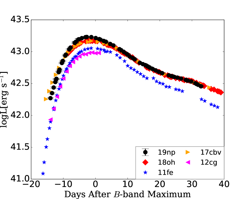
Figure 13: Quasi-bolometric light curve of SN 2019np compared to that of SNe 2018oh, 2011fe, 2012cg, and 2017cbv.

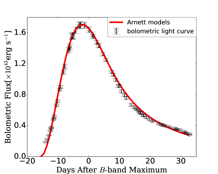
Figure 14: The quasi-bolometric light curve of SN 2019np (open black circles) compared to the best-fit radiation diffusion model (red line; Arnett 1982).

5.2 The Early-excess Flux

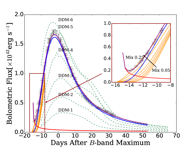
Figure 15: Bolometric light curve of SN 2019np (grey open dots) compared with various models as indicated by different color-coded curves. The solid blue line represents the radioactive decay model, and the red solid line denotes the interaction model, while the purple solid line shows the sum of the above two. DDMs are shown in green dashed lines. Six models (DDM-1 to 6) are computed for an initial CO core of the WD and He shell masses of (0.810$M_{\sun}$, 0.126$M_{\sun}$), (0.920$M_{\sun}$, 0.084$M_{\sun}$), (1.025$M_{\sun}$, 0.055$M_{\sun}$), (1.125$M_{\sun}$, 0.039$M_{\sun}$), (1.280$M_{\sun}$, 0.013$M_{\sun}$), and (1.385$M_{\sun}$, 0.0035$M_{\sun}$), respectively. The inset portrays the data and the models within the first week as the region outlined by the red square. The orange lines denote the ⁵⁶Ni mixing models; and the series of lines following the direction of the black arrow are generated using a boxcar with widths of 0.05, 0.075, 0.1, 0.125, 0.15, 0.2, and 0.25 $M_{\sun}$.

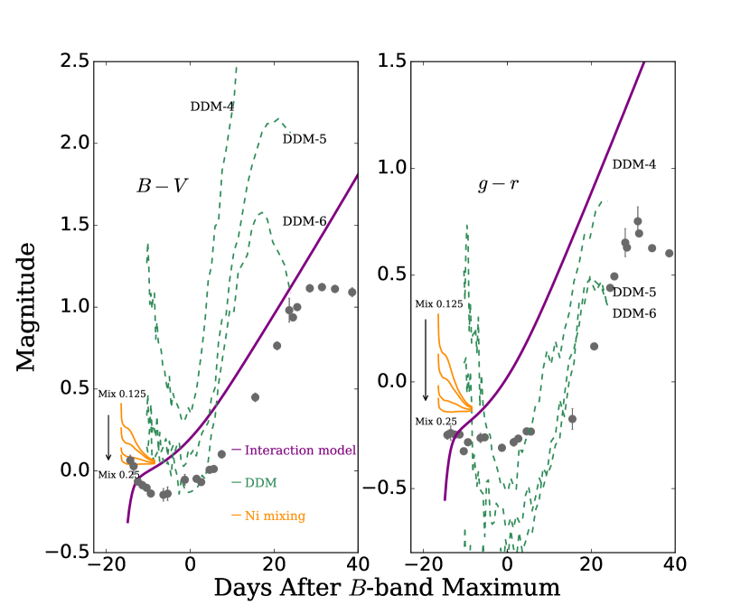
Figure 16: The $B-V$ bands (left panel) and $g-r$ bands (right panel) color of SN 2019np (grey dots) compared with various explosion models as indicated by different color-coded curves. The models are shown in the same color with Figure 15.

In Figure 14 and Figure 5, one can see that excess flux exists in the early-time light curves. Such an excess emission is hard to be explained by diffusion of centrally-located ⁵⁶Ni, but it could be related to the collision between the SN-ejecta and the companion star. Such a strong interaction would produce an optical/UV excess in the first week after the explosion. Thus, we use a hybrid model to fit the early-time light curves of SN 2019np. Assuming that the density distribution of the ejecta follows a broken power law, i.e. $\rho\propto r^{-1}$ for the inner region and $\rho\propto r^{-10}$ for the outer one, the collision-powered SN luminosity ($L_{\mathrm{col}}$) and effective temperature ($T_{\mathrm{col}}$) can be expressed as follows (Kasen, 2010):

$$L_{\mathrm{col}} \propto aM_{\mathrm{ej}}^{-5/8}E_{\mathrm{sn}}^{7/8}\kappa^{-3/4}t^{-1/2},$$ (2)

$$T_{\mathrm{col}} \propto a^{1/4}\kappa^{-35/144}t^{-37/72},$$ (3)

where $a$ is the distance between the mass center of the WD and its companion, and $t$ represents the dynamical time. We can then derive the time-dependent collision-powered flux ($F_{\nu,\mathrm{col}}$) under the assumption of blackbody radiation. For simplicity, the contribution from ⁵⁶Ni-powered radiation is described by the fireball model ($F_{nu,\mathrm{Ni}}\propto t^{2}$; Nugent et al., 2011). So the total flux can be given by $F_{\nu}=F_{\nu,\mathrm{col}}+F_{\nu,\mathrm{Ni}}$.

In this circumstance, we still set $\kappa\sim 0.085\leavevmode\nobreak\ {\rm cm^{2}\leavevmode\nobreak\ g^{-1}}$ and adopt the above fitting results ($M_{\mathrm{ej}}$, $E_{\mathrm{sn}}$) from Arnett model. Then we fit the data observed earlier than MJD 58497 and derive the best-fit parameters, which suggests that the explosion date is MJD $58495.2\pm{0.1}$ and the separation distance between the WD and its companion star ($a$) is $5.74\pm{0.38}\times 10^{11}$ cm. In most cases, the separation distance is comparable to the Roche-lobe radius of the companion star, for typical mass ratios, $a/R_{\rm companion}=2-3$ (Kasen, 2010). So the companion star could have a radius of $1.91-2.87\times 10^{11}$ cm. Thus, the corresponding companion star is likely to be a main-sequence star of $\sim 1M_{\odot}$ (see Table 1 in Kasen 2010). The best-fit result is presented in Figure 15.

In addition, there are other possible explanations for the early bump in the light curves and one particular mechanism is the ⁵⁶Ni mixing to the outermost layers (Piro & Nakar, 2013; Dimitriadis et al., 2019). In this scenario, the mass fraction of ⁵⁶Ni near the surface exceeds that in the “expanding fireball” model, which can produce extra flux, and it can happen in both SD and DD progenitor channels. A specific explosion model for such a configuration is the double-detonation sub-Chandrasekhar explosion, where the surface ⁵⁶Ni can be produced through the detonation of surface helium (Noebauer et al., 2017).

For the double detonation model (DDM), the explosion is thought to start with a shell of helium-rich material accreted by a sub-Chandrasekhar WD from its companion. The shell donation drives a shock wave that propagates towards the core of the CO WD, which could cause a secondary explosion in the core. The core explosion completely disrupts the WD (Woosley & Weaver, 1994). The DDMs 1-6, with parameters spanning from $0.810-1.385M_{\sun}$ WDs and the helium shells from $0.0035-0.126M_{\sun}$ (Kromer et al., 2010; Fink et al., 2010), are available from the Heidelberg Supernova Model Archive. We compared the bolometric light curves of SN 2019np with those predicted by the above models in Figure 15. The explosion time given by Arnett model is $t_{0}=$$58494.09\pm 0.03$d. Note, however, that the peak bolometric luminosity predicted by DDMs 4-6 is higher than the observations. In addition, the DDMs 4-6 predict a shoulder in the bolometric light curve at around $\sim 25.0$ day, which is not seen in SN 2019np.

Furthermore, it is possible that ⁵⁶Ni can also be mixed to the outer layer in some other scenarios (Piro & Nakar, 2013; Piro & Morozova, 2016). We consider a more general model in which the amount of surface ⁵⁶Ni is tuned to explore the influence on the rising light curves (Piro & Morozova, 2016). In Figure 15, we present some typical light curves given by theoretical models (Piro & Morozova, 2016) which adopted a fixed amount of ⁵⁶Ni (i.e., 0.5 $M_{\sun}$) and vary the distribution with a boxcar and a width from 0.05 to 0.25 $M_{\sun}$. As mentioned in Stritzinger et al. (2018) and Dimitriadis et al. (2019), the early-time color is an important parameter to distinguish the above models. In Figure 16, we show the color evolution of SN 2019np and the expected colors for different models. SN 2019np shows broader red-blue-red (in $B-V$ color) evolution than the DDMs. Moreover, the $g-r$ color evolution of SN 2019np is quite flat and does not conform with that predicted by the DDM. For the interaction model, the early-time color was initially blue and then became red, which is inconsistent with the observed color evolution of SN 2019np. Based on the discussions above, we conclude that the early flux excess in SN 2019np is most consistent with the ⁵⁶Ni mixing model.

6 Conclusion

We present extensive UV-optical photometry and optical-NIR spectroscopy of the Type Ia SN 2019np. The following conclusions can be made:

1) The light curves suggest that SN 2019np resembles that of other well-sampled normal SNe Ia. A $B-$band peak magnitude of $13.55\pm 0.02$  mag was reached, corresponding to an absolute magnitude of $-19.52\pm 0.47$ mag. A $B-$band luminosity decline rate is found to be $\Delta m_{\rm 15}(B)$ =$1.04\pm 0.04$ mag. Both values are consistent with the photometric behavior of normal SNe Ia;

2) We construct the quasi-bolometric light curve of SN 2019np based on the UV-optical photometry and an adoption of a NIR flux correction. The estimated peak bolometric luminosity gives $L_{\rm peak}=$$1.70\pm 0.63\times 10^{43}$ erg s^-1, indicating a synthesized nickel mass of $0.66\pm 0.05\,M_{\odot}$;

3) Photometry of SN 2019np started within the first two days of the explosion reveals an early blue bump in its lightcurves. The early bolometric flux evolution is up to $\sim$5.0% higher compared to that predicted by the diffusion of internal radiation through a homogeneous expanding ejecta (Arnett, 1982), suggesting the presence of energy sources in addition to the radioactive decay of nickel;

4) We also compare the early color evolution of SN 2019np to various models, including i) interaction between the SN ejecta and the CSM/companion star, ii) double-detonation explosion of a sub-Chandrasekhar mass WD, and iii) nickel mixed into the surface layers of the SN ejecta. We suggest that model iii) provides the most satisfactory fit;

5) NIR and nebular-phase spectra of SN 2019np show no evidence of a significant amount of Hydrogen, which is incompatible with the picture of the ejecta interacting with a nondegenerate companion or H-rich CSM.

Early observations of SNe Ia, especially those with conspicuous flux excess that deviates from radiation diffusion through a homogeneously expanding ejecta within the first few days (“early-excess SNe Ia”), play an important role in understanding the SNe Ia explosion mechanism and the nature of their progenitors (Jiang et al., 2018; Stritzinger et al., 2018). To our knowledge, only a handful of SNe Ia have been reported to show such an early excess, e.g., SNe 2012cg (Marion et al., 2016), 2013dy (Zheng et al., 2013; Zhai et al., 2016), 2017cbv (Hosseinzadeh et al., 2017; Wang et al., 2020), 2018oh (Dimitriadis et al., 2019), iPTF13dge (Ferretti et al., 2016). The ejecta of the SN Ia expand rapidly and wipe out almost all traces of the pre-explosion configuration within days after the explosion of the progenitor WD. Therefore, photometry and spectroscopy starting within days after the explosion provides a unique view of the kinematics and mean chemical composition of the outermost layers of the SN ejecta and their circumstellar environments. High-cadence monitoring is also essential to probe these properties from the outer to inner parts of the ejecta as the photosphere continuously recedes into the exploding WD. Facilitated by the alert streams of modern wide-field, high-cadence transient searches, such as the Zwicky Transient Facility (Bellm et al., 2019a, b), ATLAS (Tonry, 2011), ASAS-SN (Shappee et al., 2014), DLT40 (Tartaglia et al., 2018) and TMTS (Lin et al., 2022), rapid photometric and spectroscopic follow-up observations will provide a more comprehensive characterization of the early behaviors of SNe Ia. An extensive sample of early SNe Ia will enable stringent tests among various models that may account for the flux excess in their early luminosity evolution. It will also provide chances to test the aspect-angle dependency and uniformities of SNe Ia that belong to different subtypes.

Data availability

The data underlying this article are available in the article. Our photometric data has been attached in Table 2,  LABEL:swift and 6 in the appendix. The log tables of optical and NIR spectral data are also shown in Table 4 and Table 5.

Affiliations

¹²Millennium Institute of Astrophysics, Nuncio Monsenor Sótero Sanz 100, Providencia, Santiago 8320000, Chile
¹³George P. and Cynthia Woods Mitchell Institute for Fundamental Physics & Astronomy, Texas A. & M. University, 4242 TAMU, College Station, TX 77843, USA
¹⁴Department of Physics, Florida State University, 77 Chieftan Way, Tallahassee, FL 32306, USA
¹⁵Institut d’Estudis Espacials de Catalunya (IEEC), c/Gran Capitá 2-4, Edif. Nexus 201, 08034 Barcelona, Spain
¹⁶Itagaki Astronomical Observatory, Yamagata, Yamagata 990-2492, Japan
¹⁷The School of Physics and Astronomy, Tel Aviv University, Tel Aviv 69978, Israel
¹⁸Key Laboratory of Optical Astronomy, National Astronomical Observatories, Chinese Academy of Sciences, Beijing 100101, China
¹⁹School of Astronomy and Space Science, University of Chinese Academy of Sciences, Beijing 101408, China
²⁰Facultad de Ciencias Astronómicas y Geofísicas, Universidad Nacional de La Plata, Paseo del Bosque S/N, B1900FWA, La Plata, Argentina
²¹Carnegie Observatories, Las Campanas Observatory, Colina El Pino, Casilla 601, Chile
²²Max-Planck-Institut für Astrophysik, Karl-Schwarzschild Str. 1, 85741 Garching, Germany
²³Technische Universität München, Physik Department, James-Franck Str. 1, 85741 Garching, Germany
²⁴Department of Physics and Astronomy, Aarhus University, Ny Munkegade 120, DK-8000 Aarhus C, Denmark
²⁵Chinese Academy of Sciences South America Center for Astronomy (CASSACA), National Astronomical Observatories, CAS, Beijing 100101,
People’s Republic of China
²⁶CAS Key Laboratory of Optical Astronomy, National Astronomical Observatories, Chinese Academy of Sciences, Beijing 100101, People’s Republic of China
²⁷Department of Astronomy, The Oskar Klein Center, Stockholm University, AlbaNova, 10691 Stockholm, Sweden
²⁸Department of Astronomy, Beijing Normal University, Beijing, 100875, People’s Republic of China

Appendix A PHOTOMETRIC AND SPECTROSCOPIC DATA

Table 2: Photometric Standards in the SN 2019np Field for BVgri bands

Num.	$\alpha$(J2000)	$\delta$(J2000)	B (mag)	V (mag)	g (mag)	r (mag)	i (mag)
1	$10^{\mathrm{h}}29^{\mathrm{m}}06^{\mathrm{s}}.86$	$29\degr 30\arcmin 01\arcsec.81$	14.826(035)	14.167(012)	14.375(003)	13.969(002)	13.845(004)
2	$10^{\mathrm{h}}29^{\mathrm{m}}45^{\mathrm{s}}.12$	$29\degr 33\arcmin 23\arcsec.79$	14.446(036)	13.824(013)	14.014(007)	13.641(001)	13.527(013)
3	$10^{\mathrm{h}}29^{\mathrm{m}}16^{\mathrm{s}}.58$	$29\degr 30\arcmin 28\arcsec.17$	16.456(035)	15.745(013)	15.977(005)	15.524(002)	15.348(003)
4	$10^{\mathrm{h}}29^{\mathrm{m}}24^{\mathrm{s}}.40$	$29\degr 29\arcmin 31\arcsec.28$	16.825(035)	15.862(013)	16.213(005)	15.534(003)	15.272(002)
5	$10^{\mathrm{h}}29^{\mathrm{m}}17^{\mathrm{s}}.43$	$29\degr 25\arcmin 47\arcsec.52$	17.187(035)	16.279(014)	16.604(006)	15.974(004)	15.756(003)
6	$10^{\mathrm{h}}29^{\mathrm{m}}05^{\mathrm{s}}.83$	$29\degr 28\arcmin 26\arcsec.37$	16.281(035)	15.674(013)	15.857(004)	15.498(002)	15.390(003)
7	$10^{\mathrm{h}}29^{\mathrm{m}}22^{\mathrm{s}}.53$	$29\degr 34\arcmin 07\arcsec.31$	18.035(035)	16.958(014)	17.363(006)	16.581(004)	16.283(004)
8	$10^{\mathrm{h}}29^{\mathrm{m}}21^{\mathrm{s}}.14$	$29\degr 33\arcmin 19\arcsec.29$	17.820(035)	16.962(013)	17.264(005)	16.679(003)	16.456(002)
9	$10^{\mathrm{h}}29^{\mathrm{m}}33^{\mathrm{s}}.57$	$29\degr 34\arcmin 21\arcsec.00$	18.793(038)	17.996(021)	18.269(010)	17.739(011)	17.451(005)
10	$10^{\mathrm{h}}29^{\mathrm{m}}19^{\mathrm{s}}.68$	$29\degr 32\arcmin 25\arcsec.88$	19.127(035)	17.578(014)	18.206(006)	17.000(004)	15.672(002)
11	$10^{\mathrm{h}}29^{\mathrm{m}}33^{\mathrm{s}}.65$	$29\degr 25\arcmin 24\arcsec.47$	18.281(035)	17.325(014)	17.673(006)	17.000(004)	16.748(005)
Note: Uncertainties, in units of 0.001 mag, are $1\sigma$.

Table 3: Swift Photometry of SN 2019np

MJD	uvw2 (mag)	uvm2 (mag)	uvw1 (mag)	UVOT u (mag)	UVOT b (mag)	UVOT v (mag)
58493.7	19.644(315)	…	18.868(281)	17.091(107)	16.979(084)	16.868(123)
58494.5	19.703(255)	…	18.576(170)	16.859(085)	16.586(067)	16.415(086)
58495.7	19.156(182)	…	17.832(115)	16.295(073)	15.959(060)	15.742(069)
58497.9	18.057(114)	…	16.625(078)	14.974(055)	15.014(048)	15.012(066)
58499.7	17.125(084)	18.817(161)	15.610(063)	14.022(044)	14.473(043)	14.460(054)
58501.9	16.496(072)	17.880(104)	14.860(057)	13.300(041)	13.968(041)	14.003(048)
58502.4	16.334(068)	17.881(100)	…	…	…	…
58503.2	16.216(069)	17.552(093)	14.579(055)	13.041(040)	13.781(041)	13.805(046)
58507.8	15.925(075)	16.916(091)	14.318(055)	12.766(040)	13.443(040)	13.479(045)
58509.9	15.983(071)	17.058(086)	14.464(056)	12.896(040)	13.374(040)	13.385(044)
58511.0	16.037(072)	17.038(086)	14.536(057)	13.030(040)	13.433(040)	13.378(043)
58522.8	17.244(104)	18.048(138)	16.061(079)	14.500(050)	14.193(043)	13.783(047)
58525.7	17.653(137)	18.534(201)	16.503(101)	14.857(058)	14.475(045)	13.985(051)
58528.2	17.824(124)	18.651(179)	16.629(090)	15.168(062)	14.800(047)	14.141(051)
58531.6	18.279(156)	19.610(335)	17.070(109)	15.699(076)	15.170(051)	14.263(054)
58537.4	18.889(166)	19.647(263)	17.718(115)	16.207(073)	15.759(060)	14.624(057)
58540.9	18.882(166)	19.544(247)	17.820(121)	16.495(080)	16.050(062)	14.858(059)
58543.2	19.075(200)	19.505(263)	17.891(134)	16.590(087)	16.086(065)	14.888(062)
Note: Uncertainties, in units of 0.001 mag, are $1\sigma$.

Table 4: Log of Optical Spectroscopic Observations of SN 2019np

MJD	Phasea	Range (Å)	Resolution. (Å)	Telescope+Inst.
58493.6	-16.6	3477-8727	25	LJT+YFOSC
58493.7	-16.5	3477-8727	25	LJT+YFOSC
58495.7	-14.5	3838-8770	15	XLT+BFOSC
58496.1	-14.1	3385-9639	18	NOT+ALFOSC
58497.2	-13.0	3385-9640	18	NOT+ALFOSC
58498.2	-12.0	3385-9606	18	NOT+ALFOSC
58499.7	-10.5	3487-8730	25	LJT+YFOSC
58503.2	-7.0	3385-9639	18	NOT+ALFOSC
58506.2	-4.0	3386-9604	18	NOT+ALFOSC
58506.9	-3.3	3483-8727	25	LJT+YFOSC
58507.9	-2.4	3833-8770	15	XLT+BFOSC
58509.2	-1.1	3385-9640	18	NOT+ALFOSC
58512.1	1.9	3385-9635	18	NOT+ALFOSC
58518.7	8.5	3484-8727	25	LJT+YFOSC
58520.0	9.8	3385-9605	18	NOT+ALFOSC
58521.7	11.5	3488-8727	25	LJT+YFOSC
58522.7	12.5	4347-8665	15	XLT+BFOSC
58524.7	14.5	3485-8728	25	LJT+YFOSC
58525.6	15.4	4348-8666	15	XLT+BFOSC
58526.9	16.7	3420-9255	24	EKAR+AFOSC
58528.7	18.5	3489-8727	25	LJT+YFOSC
58536.0	25.8	3385-9606	18	NOT+ALFOSC
58539.9	29.7	3498-9256	24	EKAR+AFOSC
58543.0	32.8	3385-9253	24	EKAR+AFOSC
58548.0	37.8	3385-9242	24	EKAR+AFOSC
58552.7	42.5	3489-8729	25	LJT+YFOSC
58554.8	44.6	3841-8783	15	XLT+BFOSC
58557.1	46.9	3580-9658	18	NOT+ALFOSC
58565.8	55.6	4373-8666	15	XLT+BFOSC
58570.6	60.4	4071-8769	15	XLT+BFOSC
58571.0	60.8	3389-9246	24	EKAR+AFOSC
58601.9	91.7	3403-9650	18	NOT+ALFOSC
58608.6	98.4	4077-8772	15	XLT+BFOSC
58617.9	107.7	3402-9649	18	NOT+ALFOSC
58637.9	127.7	3484-9644	18	NOT+ALFOSC
58653.9	143.7	3534-9053	18	NOT+ALFOSC
58809.2	298.9	3891-8826	18	NOT+ALFOSC
58813.2	303.0	3813-7831	7	GTC+OSIRIS
58878.0	367.8	3833-7831	7	GTC+OSIRIS
a Days relative to the $B-$band maximum on MJD 58510.2.

Table 5: Log of NIR Spectroscopic Observations of SN 2019np

MJD	Phasea	Range (Å)	R	Telescope+Inst.
58533.2	23.0	7839-25345	450	FIRE
58566.2	56.0	6835-25343	1200	IRTF
58584.2	74.0	6844-25336	1200	IRTF
58619.0	108.8	7887-25276	450	FIRE
a Days relative to the $B-$band maximum on MJD 58510.2.

Table 6: Ground-based Optical Photometry of SN 2019np

MJD	B (mag)	V (mag)	R (mag)	I (mag)	u (mag)	g (mag)	r (mag)	i (mag)	z (mag)	data source
58492.5	…	…	…	…	…	…	18.177(131)	…	…	ZTF
58492.7	…	…	17.401(161)	…	…	…	…	…	…	BITRAN-CCD
58493.4	…	…	…	…	…	…	17.001(033)	…	…	ZTF
58493.7	16.977(043)	16.701(078)	…	…	…	16.820(060)	16.738(080)	16.950(100)	…	LJT
58494.5	…	…	…	…	…	16.356(036)	…	…	…	ZTF
58494.9	…	…	16.263(011)	16.000(022)	…	…	…	…	…	MEIA3
58495.2	16.034(027)	15.890(039)	16.229(080)	15.796(036)	…	…	…	…	…	MEIA3
58495.9	…	15.735(013)	15.797(027)	…	…	…	…	…	…	MEIA3
58495.9	15.999(021)	15.816(011)	…	…	…	15.781(010)	15.904(010)	16.157(013)	…	TNT
58496.2	15.668(023)	15.444(025)	15.545(044)	15.308(020)	…	…	…	…	…	MEIA3
58496.7	15.671(038)	15.524(014)	…	…	…	15.482(016)	15.596(018)	15.800(012)	…	TNT
58497.2	…	15.258(016)	…	…	…	…	…	…	…	MEI3A
58497.7	15.208(016)	15.155(007)	…	…	…	15.065(005)	15.186(004)	15.378(005)	…	TNT
58498.0	14.888(028)	14.977(022)	15.083(037)	14.776(024)	…	…	…	…	…	MEIAA
58498.1	14.812(019)	14.922(022)	15.060(053)	14.682(028)	…	…	…	…	…	MEIA3
58498.8	14.833(018)	14.802(006)	…	…	…	14.717(007)	14.838(005)	15.020(007)	…	TNT
58498.9	14.600(042)	14.785(044)	14.929(111)	14.547(043)	…	…	…	…	…	MEIA3
58499.0	14.409(051)	14.610(040)	14.855(111)	14.518(042)	…	…	…	…	…	MEIA3
58499.7	14.444(051)	14.544(011)	…	…	…	14.394(029)	14.644(017)	15.069(133)	…	LJT
58499.8	14.529(014)	14.514(006)	…	…	…	14.356(007)	14.555(005)	14.759(007)	…	TNT
58500.0	…	…	…	14.159(029)	…	…	…	…	…	MEIA3
58500.8	14.279(013)	14.299(006)	…	…	…	14.164(006)	14.321(006)	14.526(005)	…	TNT
58501.0	13.962(026)	14.117(028)	14.277(056)	14.009(024)	…	…	…	…	…	MEIA3
58502.0	13.695(027)	…	14.046(024)	13.846(028)	…	…	…	…	…	MEIA3
58502.4	…	…	…	…	…	13.862(020)	…	…	…	ZTF
58502.5	…	…	…	…	…	…	13.919(027)	…	…	ZTF
58503.8	13.831(026)	13.859(013)	…	…	…	13.710(014)	13.847(008)	14.076(008)	…	TNT
58504.0	…	13.726(023)	…	…	…	…	…	…	…	MEIA3
58504.1	13.491(024)	13.723(030)	13.789(057)	13.612(029)	…	…	…	…	…	MEIA3
58504.8	13.693(026)	13.714(016)	…	…	…	13.593(005)	13.727(006)	13.998(006)	…	TNT
58504.9	…	13.627(012)	…	13.511(019)	…	…	…	…	…	MEIA3
58505.0	13.403(016)	13.646(014)	13.539(022)	…	…	…	…	…	…	MEIA3
58505.1	13.395(015)	13.648(017)	13.604(038)	13.494(020)	…	…	…	…	…	MEIA3
58506.0	13.321(019)	13.684(029)	13.493(059)	13.463(024)	…	…	…	…	…	MEIA3
58506.9	13.19(0130)	13.683(035)	…	…	…	13.505(064)	14.049(085)	13.944(060)	…	LJT
58507.1	13.407(004)	13.534(003)	13.328(023)	13.491(004)	…	…	…	…	…	ALFOSC_FASU
58507.5	…	…	…	…	…	13.412(016)	…	…	…	ZTF
58508.9	13.537(022)	13.473(012)	…	…	…	13.387(009)	13.570(008)	13.985(011)	…	TNT
58510.3	…	…	…	…	…	…	13.468(026)	…	…	ZTF
58511.4	…	…	…	…	…	…	13.457(031)	…	…	ZTF
58511.7	13.518(015)	13.448(006)	…	…	…	13.383(009)	13.540(010)	14.120(007)	…	TNT
58512.8	13.520(015)	13.470(006)	…	…	…	13.416(005)	13.556(003)	14.159(006)	…	TNT
58513.4	…	…	…	…	…	…	13.491(026)	…	…	ZTF
58514.8	13.633(015)	13.508(006)	…	…	…	13.478(008)	13.584(006)	14.227(007)	…	TNT
58515.8	13.667(013)	13.537(006)	…	…	…	13.521(004)	13.628(003)	14.276(006)	…	TNT
Note: Uncertainties, in units of 0.001 mag, are $1\sigma$.

Table 7: continued

A table continued from the previous one. MJD B (mag) V (mag) R (mag) I (mag) u (mag) g (mag) r (mag) i (mag) z (mag) data source 58517.7 13.851(016) 13.631(008) … … … 13.595(009) … 14.446(006) … TNT 58518.2 13.552(015) 13.576(011) 13.630(020) … … … … … … MEIA3 58518.7 13.852(018) 13.531(043) … … … 13.844(034) 13.769(026) 14.538(033) … LJT 58519.0 13.625(017) 13.572(016) 13.698(041) 13.963(036) … … … … … MEIA3 58520.0 13.791(012) 13.637(021) 13.751(004) 14.160(004) … … … … … ALFOSC_FASU 58520.1 13.722(017) 13.679(018) 13.862(044) 14.041(028) … … … … … MEIA3 58520.8 13.930(026) 13.717(028) 14.225(077) 14.131(046) … … … … … MEIA3 58521.7 14.030(026) 13.674(024) … … … 13.963(033) 13.912(025) 14.758(024) … LJT 58521.8 13.870(017) 13.746(019) 14.070(048) 14.129(020) … … … … … MEIA3 58522.4 … … … … … 13.895(029) … … … ZTF 58524.0 14.282(036) 13.773(051) 14.382(040) 14.262(040) … … … … … MEIA3 58524.7 14.329(052) 13.874(038) … … … 14.102(026) 14.120(015) 14.881(027) … LJT 58524.9 … 13.958(020) … … … … … … … MEIA3 58525.7 14.627(020) 14.059(007) … … … 14.156(014) 14.204(035) 14.924(006) … TNT 58526.0 … … 14.083(014) 14.168(022) … … … … … MEIA3 58526.4 … … … … … 14.257(020) … … … ZTF 58526.9 14.461(067) 14.072(021) … … 15.519(024) 14.321(018) 14.208(014) 14.791(012) 14.385(014) AFOSC 58527.1 14.371(025) 14.071(027) 14.290(095) 14.141(028) … … … … … MEIA3 58527.9 … … … … 15.765(055) 14.272(028) 14.114(024) 14.852(054) … Moravian 58528.0 14.621(028) 14.219(039) … … … … … … … Moravian 58528.6 14.873(042) 14.165(030) … … … 14.369(025) 14.206(021) 14.812(023) … LJT 58528.9 14.626(025) 14.311(040) … … 15.982(055) 14.464(048) 14.218(027) 14.763(048) … Moravian 58529.9 14.852(039) 14.197(030) 14.350(079) 14.177(055) … … … … … MEIA3 58530.9 15.238(018) 14.355(007) … … … 14.642(005) 14.350(04) 14.811(006) … TNT 58530.9 15.039(044) 14.344(035) 14.251(066) 14.179(053) … … … … … MEIA3 58533.0 … 14.354(064) 14.223(067) 14.120(033) … … … … … MEIA3 58533.8 15.584(047) 14.484(027) … … … 14.941(022) … … … TNT 58534.4 … … … … … … 14.378(019) … … ZTF 58534.7 15.618(016) 14.562(007) … … … 14.996(005) 14.430(006) 14.726(007) … TNT 58535.7 15.718(015) 14.599(007) … … … 15.053(006) 14.433(005) 14.720(007) … TNT 58536.8 15.527(031) 14.607(032) … … … … … … … MEIA3 58538.3 … … … … … 15.278(031) 14.500(035) … … ZTF 58538.7 15.996(017) 14.762(007) … … … 15.313(005) 14.558(008) 14.687(007) … TNT 58538.9 15.567(016) 14.767(021) 14.362(115) 14.039(023) … … … … … MEIA3 58540.0 15.892(027) 14.801(034) 14.329(045) 14.015(022) … … … … … MEIA3 58540.0 … … … … 16.891(073) 15.405(025) 14.521(015) 14.604(018) 14.350(016) AFOSC 58540.0 15.725(057) 14.753(010) … … … … … … … AFOSC 58540.7 15.929(087) 15.035(070) … … … 15.483(056) 14.744(072) 14.950(095) … LJT 58541.3 … … … … … 15.505(031) 14.627(037) … … ZTF 58541.6 16.187(016) 14.946(007) … … … 15.526(006) 14.705(007) 14.783(007) … TNT 58542.0 15.808(035) 14.931(020) 14.559(059) 14.131(028) … … … … … MEIA3 58542.9 16.053(040) 14.905(027) 14.720(074) 14.235(042) … … … … … MEIA3 58543.0 … … … … 17.444(024) 15.562(036) 14.628(029) 14.631(034) 14.380(037) AFOSC 58543.0 15.926(034) 14.895(027) … … 17.197(043) 15.566(019) 14.744(024) 14.668(030) … Moravian 58544.0 15.913(042) 14.963(032) … … 17.238(043) 15.532(026) 14.756(027) 14.702(039) … Moravian 58544.7 16.327(016) 15.097(007) … … … 15.660(010) 14.908(006) 14.979(007) … TNT Note: Uncertainties, in units of 0.001 mag, are $1\sigma$.

Table 8: continued

A table continued from the previous one. MJD B (mag) V (mag) R (mag) I (mag) u (mag) g (mag) r (mag) i (mag) z (mag) data source 58545.1 15.984(023) 15.023(031) 14.719(060) … … … … … … MEIA3 58546.0 15.976(102) 15.073(030) … … 17.276(043) 15.696(017) 14.880(021) 14.834(018) 14.551(031) AFOSC 58547.1 16.152(037) 15.080(026) … … 17.307(117) 15.795(066) 14.973(026) 15.012(031) … Moravian 58548.0 16.171(025) 15.123(033) … … 17.455(060) 15.795(031) 15.018(033) 15.055(035) … Moravian 58548.8 16.538(020) 15.328(008) … … … 15.893(008) 15.165(009) 15.244(007) … TNT 58550.9 16.321(032) 15.361(027) 15.254(083) 14.707(040) … … … … … MEIA3 58552.7 16.478(064) 15.511(038) … … … 15.975(034) 15.407(130) 15.464(133) … LJT 58553.6 16.671(018) 15.503(007) … … … 16.045(004) 15.392(003) 15.504(009) … TNT 58553.9 16.383(032) 15.413(022) 15.308(079) 14.833(038) … … … … … MEIA3 58556.9 16.449(026) 15.487(010) 15.240(050) 14.897(018) … … … … … MEIA3 58557.1 16.400(005) 15.500(004) … … … … 15.395(015) 15.443(041) … ALFOSC_FASU 58558.2 … … … … … … 15.522(025) … … ZTF 58559.2 … … … … … … 15.539(034) … … ZTF 58559.7 16.622(089) 15.661(045) … … … 16.172(048) 15.575(032) 15.781(064) … TNT 58559.9 … 15.594(022) 15.335(051) … … … … … … MEIA3 58563.0 16.527(051) 15.549(044) 15.517(131) 15.259(053) … … … … … MEIA3 58563.5 16.873(034) 15.803(008) … … … 16.279(015) 15.757(011) 15.987(012) … TNT 58566.0 16.485(041) 15.812(042) 15.665(052) 15.446(043) … … … … … MEIA3 58566.6 16.915(016) 15.895(007) … … … 16.292(006) 15.855(007) 16.060(011) … TNT 58569.0 16.670(014) 15.776(011) 15.676(026) 15.399(023) … … … … … MEIA3 58572.0 16.615(021) 15.815(021) 15.797(053) 15.549(032) … … … … … MEIA3 58572.2 … … … … … … 15.989(027) … … ZTF 58572.5 16.972(021) 16.063(009) … … … 16.444(010) 16.067(012) 16.294(014) … TNT 58574.2 … … … … … … 16.099(057) … … ZTF 58575.2 … … … … … … 16.095(062) … … ZTF 58577.6 17.075(019) 16.179(007) … … … 16.520(007) 16.241(009) 16.490(016) … TNT 58578.0 … 16.250(042) 15.985(085) 15.857(080) … … … … … MEIA3 58580.6 … 16.250(018) … … … 16.582(009) 16.338(009) 16.620(009) … TNT 58581.1 16.812(029) 16.135(043) 16.095(109) … … … … … … MEIA3 58581.2 … … … … … … 16.271(037) … … ZTF 58582.2 … … … … … … 16.320(030) … … ZTF 58584.0 16.836(021) 16.175(013) 16.145(073) 15.977(019) … … … … … MEIA3 58584.2 … … … … … … 16.363(032) … … ZTF 58587.3 … … … … … … 16.455(024) … … ZTF 58589.6 17.24(126) 16.450(068) … … … 16.666(073) 16.687(072) 16.949(022) … TNT 58590.0 … 16.335(018) … … … … … … … MEIA3 58590.7 17.411(115) 16.414(056) … … … 16.795(092) … 16.921(026) … TNT 58591.4 … … … … … … 16.603(028) … … ZTF 58592.7 17.231(122) 16.601(042) … … … 16.811(068) 16.819(099) 16.883(060) … LJT 58593.3 … … … … … … 16.650(041) … … ZTF 58594.2 … … … … … … 16.673(042) … … ZTF 58594.7 17.242(082) 16.614(048) … … … 16.726(039) 16.701(045) 16.971(075) … TNT 58597.2 … … … … … … 16.764(044) … … ZTF 58597.4 … … … … … … 16.772(040) … … ZTF 58601.3 … … … … … … 16.891(037) … … ZTF Note: Uncertainties, in units of 0.001 mag, are $1\sigma$.

Table 9: continued

A table continued from the previous one. MJD B (mag) V (mag) R (mag) I (mag) u (mag) g (mag) r (mag) i (mag) z (mag) data source 58603.6 17.433(016) 16.793(008) … … … 16.929(009) 17.017(007) 17.391(026) … TNT 58605.5 17.392(024) 16.835(010) … … … 16.958(014) 17.118(008) 17.423(030) … TNT 58606.7 17.368(041) 16.821(027) … … … … 17.026(032) 17.282(041) … LJT 58608.2 … … … … … … 17.094(044) … … ZTF 58608.6 17.426(022) 16.946(008) … … … 17.031(009) 17.202(009) 17.519(033) … TNT 58612.2 … … … … … … 17.201(045) … … ZTF 58617.2 … … … … … … 17.327(055) … … ZTF 58618.3 … … … … … … 17.373(042) … … ZTF 58619.7 17.598(211) 17.098(052) … … … 17.281(105) 17.334(047) 17.888(046) … LJT 58623.6 17.671(031) 17.360(010) … … … 17.333(017) 17.695(009) 18.107(052) … TNT 58630.6 17.741(028) 17.475(011) … … … 17.400(017) 17.861(018) 18.310(066) … TNT 58633.6 17.789(034) 17.535(012) … … … 17.492(022) 17.931(034) 18.332(057) … TNT 58634.2 … … … … … … 17.825(067) … … ZTF 58637.2 … … … … … … 17.908(050) … … ZTF 58637.9 17.704(007) 17.469(016) … … … … 17.831(017) 18.188(024) … ALFOSC_FASU 58640.2 … … … … … … 17.971(065) … … ZTF 58645.5 17.791(131) 17.568(016) … … … 17.544(018) 18.310(015) 18.545(086) … TNT 58647.2 … … … … … … 18.145(091) … … ZTF 58648.6 18.017(072) 17.899(018) … … … 17.610(016) 18.314(025) 18.746(103) … TNT 58650.2 … … … … … … 18.194(089) … … ZTF 58653.9 17.957(031) 17.767(020) … … … … 18.270(014) 18.514(017) … ALFOSC_FASU 58816.8 … … … … … 19.115(073) 19.045(104) 19.008(080) … LJT 58929.7 … … … … … 20.307(123) 19.816(085) 19.525(086) … LJT Note: Uncertainties, in units of 0.001 mag, are $1\sigma$.

References

- Aldering et al. (2006) Aldering G., et al., 2006, ApJ, 650, 510
- Arnett (1982) Arnett W. D., 1982, ApJ, 253, 785
- Ashall et al. (2019) Ashall C., et al., 2019, ApJ, 875, L14
- Bellm et al. (2019a) Bellm E. C., et al., 2019a, PASP, 131, 018002
- Bellm et al. (2019b) Bellm E. C., et al., 2019b, PASP, 131, 068003
- Benetti et al. (2005) Benetti S., et al., 2005, ApJ, 623, 1011
- Benz et al. (1990) Benz W., Bowers R. L., Cameron A. G. W., Press W. H. ., 1990, ApJ, 348, 647
- Burns et al. (2011) Burns C. R., et al., 2011, AJ, 141, 19
- Burns et al. (2018) Burns C. R., et al., 2018, ApJ, 869, 56
- Cardelli et al. (1989) Cardelli J. A., Clayton G. C., Mathis J. S., 1989, ApJ, 345, 245
- Chatzopoulos et al. (2012) Chatzopoulos E., Wheeler J. C., Vinko J., 2012, ApJ, 746, 121
- Chatzopoulos et al. (2013) Chatzopoulos E., Wheeler J. C., Vinko J., Horvath Z. L., Nagy A., 2013, ApJ, 773, 76
- Clocchiatti & Wheeler (1997) Clocchiatti A., Wheeler J. C., 1997, ApJ, 491, 375
- Cushing et al. (2004) Cushing M. C., Vacca W. D., Rayner J. T., 2004, PASP, 116, 362
- Dilday et al. (2012) Dilday B., et al., 2012, Science, 337, 942
- Dimitriadis et al. (2019) Dimitriadis G., et al., 2019, ApJ, 870, L1
- Ferretti et al. (2016) Ferretti R., et al., 2016, A&A, 592, A40
- Fink et al. (2010) Fink M., Röpke F. K., Hillebrandt W., Seitenzahl I. R., Sim S. A., Kromer M., 2010, A&A, 514, A53
- Fukugita et al. (1996) Fukugita M., Ichikawa T., Gunn J. E., Doi M., Shimasaku K., Schneider D. P., 1996, AJ, 111, 1748
- Gehrels et al. (2004) Gehrels N., et al., 2004, ApJ, 611, 1005
- González Hernández et al. (2012) González Hernández J. I., Ruiz-Lapuente P., Tabernero H. M., Montes D., Canal R., Méndez J., Bedin L. R., 2012, Nature, 489, 533
- Guy et al. (2005) Guy J., Astier P., Nobili S., Regnault N., Pain R., 2005, A&A, 443, 781
- Guy et al. (2010) Guy J., et al., 2010, A&A, 523, A7
- Haas et al. (2010) Haas M. R., et al., 2010, ApJ, 713, L115
- Hamuy et al. (2003) Hamuy M., et al., 2003, Nature, 424, 651
- Hosseinzadeh et al. (2017) Hosseinzadeh G., et al., 2017, ApJ, 845, L11
- Howell (2011) Howell D. A., 2011, Nature Communications, 2, 350
- Howell et al. (2006) Howell D. A., et al., 2006, Nature, 443, 308
- Hsiao et al. (2013) Hsiao E. Y., et al., 2013, ApJ, 766, 72
- Hsiao et al. (2015) Hsiao E. Y., et al., 2015, A&A, 578, A9
- Hsiao et al. (2019) Hsiao E. Y., et al., 2019, PASP, 131, 014002
- Huang et al. (2012) Huang F., Li J.-Z., Wang X.-F., Shang R.-C., Zhang T.-M., Hu J.-Y., Qiu Y.-L., Jiang X.-J., 2012, Research in Astronomy and Astrophysics, 12, 1585
- Iben & Tutukov (1984) Iben I. J., Tutukov A. V., 1984, ApJS, 54, 335
- Jha et al. (2019) Jha S. W., Maguire K., Sullivan M., 2019, Nature Astronomy, 3, 706
- Jiang et al. (2018) Jiang J.-a., Doi M., Maeda K., Shigeyama T., 2018, ApJ, 865, 149
- Jiang et al. (2021) Jiang J.-a., et al., 2021, ApJ, 923, L8
- Johnson et al. (1966) Johnson H. L., Mitchell R. I., Iriarte B., Wisniewski W. Z., 1966, Communications of the Lunar and Planetary Laboratory, 4, 99
- Kasen (2010) Kasen D., 2010, ApJ, 708, 1025
- Kilpatrick & Foley (2019) Kilpatrick C. D., Foley R. J., 2019, The Astronomer’s Telegram, 12375, 1
- Kromer et al. (2010) Kromer M., Sim S. A., Fink M., Röpke F. K., Seitenzahl I. R., Hillebrandt W., 2010, ApJ, 719, 1067
- Kushnir et al. (2013) Kushnir D., Katz B., Dong S., Livne E., Fernández R., 2013, ApJ, 778, L37
- Leonard (2007) Leonard D. C., 2007, ApJ, 670, 1275
- Li et al. (2011) Li W., et al., 2011, Nature, 480, 348
- Li et al. (2019) Li W., et al., 2019, ApJ, 870, 12
- Lin et al. (2022) Lin J., et al., 2022, MNRAS, 509, 2362
- Magee et al. (2020) Magee M. R., Maguire K., Kotak R., Sim S. A., Gillanders J. H., Prentice S. J., Skillen K., 2020, A&A, 634, A37
- Maguire et al. (2013) Maguire K., et al., 2013, MNRAS, 436, 222
- Maguire et al. (2016) Maguire K., Taubenberger S., Sullivan M., Mazzali P. A., 2016, MNRAS, 457, 3254
- Maoz et al. (2014) Maoz D., Mannucci F., Nelemans G., 2014, ARA&A, 52, 107
- Marion et al. (2016) Marion G. H., et al., 2016, ApJ, 820, 92
- Mattila et al. (2005) Mattila S., Lundqvist P., Sollerman J., Kozma C., Baron E., Fransson C., Leibundgut B., Nomoto K., 2005, A&A, 443, 649
- Mazzali et al. (2014) Mazzali P. A., et al., 2014, MNRAS, 439, 1959
- Noebauer et al. (2017) Noebauer U. M., Kromer M., Taubenberger S., Baklanov P., Blinnikov S., Sorokina E., Hillebrandt W., 2017, MNRAS, 472, 2787
- Nomoto et al. (1997) Nomoto K., Iwamoto K., Kishimoto N., 1997, Science, 276, 1378
- Nugent et al. (2011) Nugent P. E., et al., 2011, Nature, 480, 344
- Olling et al. (2015) Olling R. P., et al., 2015, Nature, 521, 332
- Pakmor et al. (2012) Pakmor R., Kromer M., Taubenberger S., Sim S. A., Röpke F. K., Hillebrandt W., 2012, ApJ, 747, L10
- Pan et al. (2015) Pan Y. C., et al., 2015, MNRAS, 452, 4307
- Patat et al. (2007) Patat F., et al., 2007, Science, 317, 924
- Perlmutter et al. (1999) Perlmutter S., et al., 1999, ApJ, 517, 565
- Phillips et al. (1999) Phillips M. M., Lira P., Suntzeff N. B., Schommer R. A., Hamuy M., Maza J., 1999, AJ, 118, 1766
- Phillips et al. (2013) Phillips M. M., et al., 2013, ApJ, 779, 38
- Piro & Morozova (2016) Piro A. L., Morozova V. S., 2016, ApJ, 826, 96
- Piro & Nakar (2013) Piro A. L., Nakar E., 2013, ApJ, 769, 67
- Podsiadlowski et al. (2008) Podsiadlowski P., Mazzali P., Lesaffre P., Han Z., Förster F., 2008, New Astron. Rev., 52, 381
- Poznanski et al. (2012) Poznanski D., Prochaska J. X., Bloom J. S., 2012, MNRAS, 426, 1465
- Rayner et al. (2003) Rayner J. T., Toomey D. W., Onaka P. M., Denault A. J., Stahlberger W. E., Vacca W. D., Cushing M. C., Wang S., 2003, PASP, 115, 362
- Riess et al. (1996) Riess A. G., Press W. H., Kirshner R. P., 1996, ApJ, 473, 88
- Riess et al. (1998) Riess A. G., et al., 1998, AJ, 116, 1009
- Riess et al. (2016) Riess A. G., et al., 2016, ApJ, 826, 56
- Riess et al. (2018) Riess A. G., et al., 2018, ApJ, 853, 126
- Riess et al. (2021) Riess A. G., et al., 2021, arXiv e-prints, p. arXiv:2112.04510
- Roming et al. (2005) Roming P. W. A., et al., 2005, Space Sci. Rev., 120, 95
- Sand et al. (2018) Sand D. J., et al., 2018, ApJ, 863, 24
- Schaefer & Pagnotta (2012) Schaefer B. E., Pagnotta A., 2012, Nature, 481, 164
- Schlafly & Finkbeiner (2011) Schlafly E. F., Finkbeiner D. P., 2011, ApJ, 737, 103
- Shappee et al. (2013) Shappee B. J., Stanek K. Z., Pogge R. W., Garnavich P. M., 2013, ApJ, 762, L5
- Shappee et al. (2014) Shappee B., et al., 2014, in American Astronomical Society Meeting Abstracts #223. p. 236.03
- Shappee et al. (2019) Shappee B. J., et al., 2019, ApJ, 870, 13
- Silverman et al. (2012) Silverman J. M., et al., 2012, MNRAS, 425, 1789
- Silverman et al. (2013) Silverman J. M., et al., 2013, ApJS, 207, 3
- Simcoe et al. (2013) Simcoe R. A., et al., 2013, PASP, 125, 270
- Stahl et al. (2019) Stahl B. E., et al., 2019, MNRAS, 490, 3882
- Sternberg et al. (2011) Sternberg A., et al., 2011, Science, 333, 856
- Stritzinger et al. (2018) Stritzinger M. D., et al., 2018, ApJ, 864, L35
- Tartaglia et al. (2018) Tartaglia L., et al., 2018, ApJ, 853, 62
- Tonry (2011) Tonry J. L., 2011, PASP, 123, 58
- Toonen et al. (2018) Toonen S., Perets H. B., Hamers A. S., 2018, A&A, 610, A22
- Tsvetkov et al. (2013) Tsvetkov D. Y., Shugarov S. Y., Volkov I. M., Goranskij V. P., Pavlyuk N. N., Katysheva N. A., Barsukova E. A., Valeev A. F., 2013, Contributions of the Astronomical Observatory Skalnate Pleso, 43, 94
- Tucker et al. (2019) Tucker M. A., Shappee B. J., Wisniewski J. P., 2019, ApJ, 872, L22
- Tucker et al. (2020) Tucker M. A., et al., 2020, MNRAS, 493, 1044
- Tully et al. (2016) Tully R. B., Courtois H. M., Sorce J. G., 2016, AJ, 152, 50
- Valenti et al. (2008) Valenti S., et al., 2008, MNRAS, 383, 1485
- Wang & Han (2012) Wang B., Han Z., 2012, New Astron. Rev., 56, 122
- Wang et al. (2005) Wang X., Wang L., Zhou X., Lou Y.-Q., Li Z., 2005, ApJ, 620, L87
- Wang et al. (2009a) Wang B., Meng X., Chen X., Han Z., 2009a, MNRAS, 395, 847
- Wang et al. (2009b) Wang X., et al., 2009b, ApJ, 697, 380
- Wang et al. (2009c) Wang X., et al., 2009c, ApJ, 699, L139
- Wang et al. (2013a) Wang X., Wang L., Filippenko A. V., Zhang T., Zhao X., 2013a, Science, 340, 170
- Wang et al. (2013b) Wang B., Justham S., Han Z., 2013b, A&A, 559, A94
- Wang et al. (2020) Wang L., et al., 2020, ApJ, 904, 14
- Wang et al. (2021) Wang Q., et al., 2021, ApJ, 923, 167
- Webbink (1984) Webbink R. F., 1984, ApJ, 277, 355
- Wheeler et al. (1998) Wheeler J. C., Höflich P., Harkness R. P., Spyromilio J., 1998, ApJ, 496, 908
- Wheeler et al. (2015) Wheeler J. C., Johnson V., Clocchiatti A., 2015, MNRAS, 450, 1295
- Whelan & Iben (1973) Whelan J., Iben Icko J., 1973, ApJ, 186, 1007
- Woosley & Weaver (1994) Woosley S. E., Weaver T. A., 1994, ApJ, 423, 371
- Wu et al. (2019) Wu C., Zhang J., Wang X., Huang F., 2019, The Astronomer’s Telegram, 12374, 1
- Yaron & Gal-Yam (2012) Yaron O., Gal-Yam A., 2012, PASP, 124, 668
- Zeng et al. (2021) Zeng X., et al., 2021, ApJ, 919, 49
- Zhai et al. (2016) Zhai Q., et al., 2016, AJ, 151, 125
- Zhang et al. (2016a) Zhang J.-C., Fan Z., Yan J.-Z., Bharat Kumar Y., Li H.-B., Gao D.-Y., Jiang X.-J., 2016a, PASP, 128, 105004
- Zhang et al. (2016b) Zhang K., et al., 2016b, ApJ, 820, 67
- Zheng et al. (2013) Zheng W., et al., 2013, ApJ, 778, L15