QuanEstimation: An open-source toolkit for quantum parameter estimation

Abstract

Quantum parameter estimation promises a high-precision measurement in theory; however, how to design the optimal scheme in a specific scenario, especially under a practical condition, is still a serious problem that needs to be solved case by case due to the existence of multiple mathematical bounds and optimization methods. Depending on the scenario considered, different bounds may be more or less suitable, both in terms of computational complexity and the tightness of the bound itself. At the same time, the metrological schemes provided by different optimization methods need to be tested against realization complexity, robustness, etc. Hence, a comprehensive toolkit containing various bounds and optimization methods is essential for the scheme design in quantum metrology. To fill this vacancy, here we present a Python-Julia-based open-source toolkit for quantum parameter estimation, which includes many well-used mathematical bounds and optimization methods. Utilizing this toolkit, all procedures in the scheme design, such as the optimizations of the probe state, control and measurement, can be readily and efficiently performed.

I Introduction

Quantum metrology is an emerging cross-disciplinary field between precision measurement and quantum technology, and has now become one of the most promising fields in quantum technology due to the general belief that it could step into the industrial-grade applications in a short time [1, 2, 3, 4, 5]. Meanwhile, its development not only benefits the applied technologies like the magnetometry, thermometry, and gravimetry, but also the studies in fundamental physics such as the detection of gravitational waves [6] and the search of dark matters [7, 8]. As the theoretical support of quantum metrology, quantum parameter estimation started from 1960s [9], and has become an indispensable component of quantum metrology nowadays [10, 11, 12, 13, 14, 15, 16, 17, 18].

One of the key challenges in quantum parameter estimation is to design optimal schemes with quantum apparatuses and quantum resources, leading to enhanced precision when compared with their classical counterparts. A typical scheme in quantum parameter estimation usually contains four steps: (1) preparation; (2) parameterization; (3) measurement; and (4) classical estimation. The first step is the preparation of the probe state. The parameters to be estimated are involved in the second step, which is also known as sensing in the field of quantum sensing. With the parameterized state given in the second step, the third step is to perform the quantum measurement, which results in a set of probability distributions. Estimating the unknown parameters from the obtained probability distributions is finished in the last step. The design of an optimal scheme usually requires the optimizations of some or all of the steps above.

In quantum parameter estimation, there exist various mathematical bounds to depict the theoretical precision limit. Depending on the type of the bound considered, it will be more or less informative depending on the type of estimation scenario considered, be it: single-shot versus many-repetition scenario, single versus multiple-parameter scenario, etc. Moreover, by choosing different objective functions when optimizing quantum estimation schemes, one may arrive at solutions with contrastingly different robustness properties, complexity of practical implementation and so on. Hence, the design of optimal schemes has to be performed case by case most of the time. This is the reason why a general quantum parameter estimation toolkit is needed. In the meantime, thanks to the fast development of quantum metrology and its promising future, many scientists working on specific physical systems, such as the nitrogen-vacancy centers, quantum circuits, trapped ions, and atoms, are also eager to use the cutting-edge technologies in quantum parameter estimation for the design of metrological schemes on their platforms. The existence of a comprehensive toolkit will definitely reduce the technical difficulty for them to fulfill this mission and greatly improve the efficiency of research. Therefore, developing such a toolkit is the major motivation of this paper.

Currently, there exist many useful toolkits based on various coding platforms in quantum information. A famous one is the QuTiP developed by Johansson, Nation, and Nori [19, 20] in 2012, which can execute many basic calculations in quantum information. In the field of quantum control, Machnes et al. [21] developed DYNAMO and Hogben et al. developed Spinach [22] based on Matlab. Goerz et al. developed Krotov [23], which owns three versions based on Fortran, Python, and Julia, respectively. Günther et al. developed Quandary [24] based on C++. Moreover, there exist other packages like Kwant [25] for quantum transport and ProjectQ [26] for quantum computing. In quantum metrology, Chabuda and Demkowicz-Dobrzański developed TNQMetro [27], a tensor-network based Python package to perform efficient quantum metrology computations.

Hereby we present a new numerical toolkit, QuanEstimation, based on both Python and Julia for the quantum parameter estimation and provide some examples to demonstrate its usage and performance. QuanEstimation is designed to fill the lack of a general toolkit in quantum parameter estimation, not a general one in quantum information. Hence, it only focuses on the missions in quantum parameter estimation, and the main features are significantly different from the existing toolkits in quantum information. Specifically, it contains several widely-used metrological tools, such as the asymptotic Fisher information based quantities as well as their Bayesian counterparts (including direct Bayesian cost minimization, Bayesian versions of the classical and quantum Cramér-Rao bounds as well as the quantum Ziv-Zakai bound). For the sake of scheme design, QuanEstimation can execute the optimizations of the probe state, control, and measurement, as well as the simultaneous optimizations among them with both gradient-based and gradient-free methods. Due to the fact that most of the time adaptive measurement schemes are the best practical way to realize the asymptotic advantage indicated by the quantum Fisher information, QuanEstimation can also execute online adaptive measurement schemes, such as the adaptive phase estimation, and provide the real-time values of the tunable parameters that can be directly used in an experiment.

II Overview

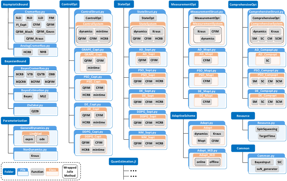
Figure 1: Schematic of the package structure of QuanEstimation. The blue boxes and the light blue boxes represent the folders and the files. The orange boxes and the gray boxes represent the classes and the functions/methods. The boxes circled by the dotted lines represents the wrapped Julia methods, which are solved in Julia scripts.

QuanEstimation is a scientific computing package focusing on the calculations and optimizations in quantum parameter estimation. It is based on both Python and Julia. The interface is written in Python due to the fact that nowadays Python is one of the most popular platforms for scientific computing. However, QuanEstimation contains many optimization processes which need to execute massive numbers of elementary processes such as the loops. These elementary processes could be very time-consuming in Python, and thus strongly affect the efficiency of the optimizations. This is why Julia is involved in this package. Julia has many wonderful features, such as optional typing and multiple dispatch, and these features let the loop and other calculation processes cost way less time than those in Python. Hence, the optimizations in QuanEstimation are all performed in Julia. Nevertheless, currently the community of Julia is not comparable to that of Python, and the hybrid structure of this package would allow the people who are not familiar with Julia use the package without any obstacle. In the meantime, QuanEstimation has a full Julia version for the users experienced in Julia.

The package structure of QuanEstimation is illustrated in Fig. 1. The blue boxes and the light blue boxes represent the folders and the files. The orange boxes and the gray boxes represent the classes and the functions/methods. The boxes circled by the dotted lines represents the wrapped Julia methods, which are solved in Julia, namely, this part of calculation are sent to Julia to execute.

The functions for the calculation of the parameterization process and dynamics are in the folder named "Parameterization". In this folder, the file "GeneralDynamics.py" contains the functions to solve the Lindblad-type master equation. Currently, the master equation can be solved directly, i.e., solving the corresponding ordinary differential equation, or via the matrix exponential. To improve the efficiency, the calculation of the dynamics via the matrix exponential are executed in Julia and when the calculation is finished, the data is sent back to Python for further use. The file "NonDynamics.py" contains the non-dynamical methods for the parameterization, which currently includes the description via Kraus operators. Details and the usage of these functions will be thoroughly introduced in Sec. III.

The functions for the calculation of the metrological tools and bounds are distributed in two folders named "AsymptoticBound" and "BayesianBound". In the folder "AsymptoticBound", the file "CramerRao.py" contains the functions to calculate the quantities related to the quantum Cramér-Rao bounds, and the file "AnalogCramerRao.py" contains those to calculate the Holevo-type quantum Cramér-Rao bound and Nagaoka-Hayashi bound. In the folder "BayesianBound", the file "BayesCramerRao.py" contains the functions to calculate several versions of the Bayesian classical and quantum Cramér-Rao bounds and "ZivZakai.py" contains the function to calculate the quantum Ziv-Zakai bound. The file "BayesEstimation.py" contains the functions to execute the Bayesian estimation and the maximum likelihood estimation. The aforementioned metrological tools and the corresponding rules to call them will be given in Sec. IV.

The functions for the calculation of metrological resources are placed in the folder named "Resource". In this folder, the file "Resource.py" currently contains two types of resources, the spin squeezing and the target time to reach a given value of an objective function, which will be thoroughly introduced in Sec. V. The resources that can be readily calculated via QuTiP [19, 20] are not included at this moment.

The scripts for the control optimization, state optimization, measurement optimization, and comprehensive optimization are in the folders named "ControlOpt", "StateOpt", "MeasurementOpt", and "ComprehensiveOpt", respectively. The structures of these folders are basically the same, and here we only take the folder of "ControlOpt" as an demonstration to explain the basic structure. In this folder, the file "ControlStruct.py" contains a function named ControlOpt() and a class named ControlSystem(). The function ControlOpt() is used to receive the initialized parameters given by the user, and then delivers them to one of the classes in the files "GRAPE_Copt.py", "PSO_Copt.py", "DE_Copt.py", and "DDPG_Copt.py" according to the user’s choice of the algorithm. These classes inherit the attributes in ControlSystem(). Then based on the choice of the objective function, the related parts in ControlSystem() is called in these classes to further run the scripts in Julia. ControlSystem() contains all the common parts that different algorithms would use and the interface with the scripts in Julia. This design is to avoid the repetition code in the algorithm files and let the extension neat and simple when more algorithms need to be included in the future. The usage of QuanEstimation for control optimization, state optimization, measurement optimization, and comprehensive optimization, as well as the corresponding illustrations will be thoroughly discussed in Secs. VI, VII, VIII, and IX, respectively.

The scripts for the adaptive measurement are in the folder named "AdaptiveScheme". In this folder, the file "Adapt.py" contains the class to execute the adaptive measurement scheme, and "Adapt_MZI.py" contains the class to generate online and offline adaptive schemes in the Mach-Zehnder interferometer. The details of the adaptive scheme and how to perform it with QuanEstimation will be given in Sec. X.

The folder "Common" contains some common functions that are regularly called in QuanEstimation. Currently it contains three functions. SIC() is used to generate a set of rank-one symmetric informationally complete positive operator-valued measure. suN_generator() is used to generate a set of su($N$) generators. BayesInput() is used to generate a legitimate form of Hamiltonian (or a set of Kraus operators) and its derivative, which can be used as the input in some functions in "BayesEstimation.py" and "Adapt.py".

All the Julia scripts are wrapped up as an independent Julia package named "QuanEstimation.jl", which has already been added in the official Julia registry and can be directly called in Julia via using QuanEstimation. One design principle of QuanEstimation for the optimizations is that once the calculation goes into the parts in Julia, it will stay in Julia until all the calculations are finished and data generated. Hence, "QuanEstimation.jl" also contains the scripts to calculate the metrological tools and resources for the sake of internal calling in Julia. To keep a high extendability, the optimizations are divided into four elements in Julia, including the scenario of optimization, the algorithm, the parameterization process and the objective function, which are distributed in the files "OptScenario.jl", "Algorithm.jl", "Parameterization.jl", and "ObjectiveFunc.jl" in the folders "OptScenario", "Algorithm", "Parameterization", and "ObjectiveFunc", respectively. Once the information and parameter settings of all elements are input by the user, they are sent to the file "run.jl", which is further used to execute the program.

Similar to other packages, the usage of QuanEstimation requires the existence of some other packages in the environment. In python it requires the pre-installation of numpy, scipy, sympy, cvxpy, and more-itertools. In Julia it requires the pre-installation of LinearAlgebra, Zygote, Convex, SCS, ReinforcementLearning, SparseArrays, DelimitedFiles, StatsBase, BoundaryValueDiffEq, Random, Trapz, Interpolations, Printf, IntervalSets, StableRNGs, Flux, Distributions, DifferentialEquations, and QuadGK. The calling of the package in Python can be done with the following line of code:

⬇

from quanestimation import *

All the scripts demonstrated in the following are based on this calling form.

III Parameterization process

The parameterization process is a key step in the quantum parameter estimation, and in physical terms this process corresponds to a parameter dependent quantum dynamics. Hence, the ability to solve the dynamics is an indispensable element of numerical calculations in quantum parameter estimation. In QuanEstimation, we mainly focus on the dynamics governed by the quantum master equation

$$\partial_{t}\rho =\mathcal{L}\rho$$

$$=-i[H,\rho]+\sum_{i}\gamma_{i}\left(\Gamma_{i}\rho\Gamma^{\dagger}_{i}-\frac{1}{2}\left\{\rho,\Gamma^{\dagger}_{i}\Gamma_{i}\right\}\right),$$ (1)

where $\rho$ is the evolved density matrix, $H$ is the Hamiltonian of the system, and $\Gamma_{i}$ and $\gamma_{i}$ are the $i$th decay operator and decay rate, respectively. Here $\gamma_{i}$ could either be fixed or time-dependent. The total Hamiltonian $H$ includes two terms, the free Hamiltonian $H_{0}(\mathbb{x})$, which is a function of the parameters $\mathbb{x}$, and control Hamiltonian $H_{\mathrm{c}}$. In the quantum parameter estimation, most calculations require the dynamical information of $\rho$ and its derivatives with respect to $\mathbb{x}$, which is denoted by $\partial_{\mathbb{x}}\rho:=(\partial_{0}\rho,\partial_{1}\rho,\dots)$ with $\partial_{a}$ short for $\partial_{x_{a}}$. Hence, in the package $\rho$ and $\partial_{\mathbb{x}}\rho$ can be solved simultaneously via the code:

⬇

dynamics = Lindblad(tspan,rho0,H0,dH,

decay=[],Hc=[],ctrl=[])

rho,drho = dynamics.expm()

Here the input tspan is an array representing the time length for the evolution and rho0 is a matrix representing the initial (probe) state. H0 is a matrix or a list of matrices representing the free Hamiltonian. It is a matrix when the free Hamiltonian is time-independent and a list (the length equals to that of tspan) when it is time-dependent. dH is a list containing the derivatives of $H_{0}(\mathbb{x})$ on $\mathbb{x}$, i.e., $[\partial_{a}H_{0},\partial_{b}H_{0},\dots]$. decay is a list including both decay operators and decay rates, and its input rule is decay=[[Gamma1,gamma1],[Gamma2,gamma2],…], where Gamma1 (Gamma2) and gamma1 (gamma2) represent $\Gamma_{1}$ ($\Gamma_{2}$) and $\gamma_{1}$ ($\gamma_{2}$), respectively. gamma1 (gamma2) could be either a float number (representing a fixed decay rate) or an array (representing a time-dependent decay rate), and when it is an array, its length should be the same with tspan. Currently all the length of the decay rates should be the same, i.e., all be float numbers or arrays with the same length. The default value is empty, which means the dynamics is unitary. Hc is a list of matrices representing the control Hamiltonians and when it is empty, the dynamics is only governed by the free Hamiltonian. ctrl (default value is empty) is a list of arrays containing the control amplitudes with respect the control Hamiltonians in Hc. The output rho is a list representing density matrices in the dynamics. drho is also a list and its $i$th entry is a list containing all derivatives $\partial_{\mathbb{x}}\rho$ at $i$th time interval. Moreover, dynamics.expm() in this demonstrating code means the dynamics is solved by the matrix exponential, i.e., the density matrix at $j$th time interval is calculated via $\rho_{j}=e^{\Delta t_{j}\mathcal{L}}\rho_{j-1}$ with $\Delta t_{j}$ a small time interval and $\rho_{j-1}$ the density matrix at the previous time interval. $\partial_{\mathbb{x}}\rho_{j}$ is solved by the iterative equation

$$\partial_{\mathbb{x}}\rho_{j} =\Delta t_{j}(\partial_{\mathbb{x}}\mathcal{L})\rho_{j}+e^{\Delta t_{j}\mathcal{L}}(\partial_{\mathbb{x}}\rho_{j-1})$$

$$=-i\Delta t_{j}[\partial_{\mathbb{x}}H_{0},\rho_{j}]+e^{\Delta t_{j}\mathcal{L}}(\partial_{\mathbb{x}}\rho_{j-1}).$$ (2)

Here the decay operators and decay rates are assumed to be independent of $\mathbb{x}$. In this method $\Delta t_{j}$ is automatically obtained by calculating the difference between the $j$th and $(j-1)$th entries in tspan. The numerical accuracy of the equation above is limited by the set of $\{\Delta t_{j}\}$, indicating that a smaller $\{\Delta t_{j}\}$ would always benefit the improvement of the accuracy in general. However, a smaller $\{\Delta t_{j}\}$ also means a larger number of calculation steps for a fixed evolution time, resulting in a greater time consumption. Hence, in practice a reasonable values of $\{\Delta t_{j}\}$ should be chosen to balance the accuracy and time consumption.

Alternatively, the dynamics can also be solved by directly solving the ordinary differential equation (ODE) in Eq. (1), which can be realized by replacing dynamics.expm() with dynamics.ode() in the demonstrating code. In this method, $\partial_{\mathbb{x}}\rho$ is solved by the equation

$$\partial_{t}(\partial_{\mathbb{x}}\rho)=-i\left[\partial_{\mathbb{x}}H,\rho\right]+\mathcal{L}\left(\partial_{\mathbb{x}}\rho\right).$$ (3)

The calculation of metrological bounds, which will be discussed in the next section, does not rely on the calling of above intrinsic dynamics in the package as they only require the input of $\rho$ and $\partial_{\mathbb{x}}\rho$ (and other essential parameters), not any dynamical information. Hence, the dynamics can also be solved by other packages like QuTiP [19, 20].

In certain cases, the parameterization process can be described by some non-dynamical methods, such as the Kraus operators. In this case, the parameterized density matrix can be expressed by

$$\rho(\mathbb{x})=\sum_{i}K_{i}(\mathbb{x})\rho_{0}K_{i}^{\dagger}(\mathbb{x}),$$ (4)

where $K_{i}(\mathbb{x})$ is a Kraus operator satisfying $\sum_{i}K^{\dagger}_{i}K_{i}=\openone$ with $\openone$ the identity operator, $\rho_{0}$ is the probe state which is independent of the unknown parameters. In QuanEstimation, $\rho$ and $\partial_{\mathbb{x}}\rho$ obtained from Kraus operators can be solved via the code:

⬇

rho,drho = Kraus(rho0,K,dK)

Here rho0 is a matrix representing the probe state, K is a list of matrices with each entry a Kraus operator, and dK is a list with $i$th entry also a list representing the derivatives $\partial_{\mathbb{x}}K_{i}$.

The aforementioned functions only calculate $\rho$ and $\partial_{\mathbb{x}}\rho$ at a fixed point of $\mathbb{x}$. However, in the Bayesian scenarios, the values of $\rho$ and $\partial_{\mathbb{x}}\rho$ with respect to a regime of $\mathbb{x}$ may be in need. In this case, if the users can provide the specific functions of $H$ and $\partial_{\mathbb{x}}H$, or Kraus operators $\{K_{i}\}$ and derivatives $\{\partial_{\mathbb{x}}K_{i}\}$, the variables H, dH (or K, dK) can be generated by the function

⬇

H0,dH = BayesInput(x,func,dfunc,

channel="dynamics")

Here x is a list of arrays representing the regime of $\mathbb{x}$. H0 is a list of matrices representing the free Hamiltonian with respect to the values in x, and it is multidimensional in the case that x has more than one entry. dH is a (multidimensional) list with each entry also a list representing $\partial_{\mathbb{x}}H$ with respect to the values in x. func and dfunc are the handles of the functions func() and dfunc(), which are defined by the users representing $H(\mathbb{x})$ and $\partial_{\mathbb{x}}H(\mathbb{x})$. Notice that the output of dfunc() should also be a list representing $[\partial_{0}H,\partial_{1}H,\dots]$. The output of BayesInput() can be switched between H, dH and K, dK by setting channel="dynamics" or channel="Kraus". After calling BayesInput(), $\rho$ and $\partial_{\mathbb{x}}\rho$ can be further obtained via the calling of Lindblad() and Kraus().

IV Quantum metrological tools

In this section, we will briefly introduce the metrological tools that have been involved in QuanEstimation and demonstrate how to calculate them with our package. Both asymptotic and Bayesian tools are included, such as the quantum Cramér-Rao bounds, Holevo Cramér-Rao bound, Nagaoka-Hayashi bound, Bayesian estimation, and Bayesian type of Cramér-Rao bounds like Van Trees bound and Tsang-Wiseman-Caves bound.

IV.1 Quantum Cramér-Rao bounds

Quantum Cramér-Rao bounds [28, 29] are the most renown metrological tools in quantum parameter estimation. Let $\rho=\rho(\mathbb{x})$ be a parameterized density matrix and $\{\Pi_{y}\}$ a set of positive operator-valued measure (POVM), then the covariance matrix $\mathrm{cov}(\hat{\mathbb{x}},\{\Pi_{y}\}):=\sum_{y}\mathrm{Tr}(\rho\Pi_{y})(\hat{\mathbb{x}}-\mathbb{x})(\hat{\mathbb{x}}-\mathbb{x})^{\mathrm{T}}$ for the unknown parameters $\mathbb{x}=(x_{0},x_{1},\dots)^{\mathrm{T}}$ and the corresponding unbiased estimators $\hat{\mathbb{x}}=(\hat{x}_{0},\hat{x}_{1},\dots)^{\mathrm{T}}$ satisfies the following inequalities [28, 29]

$$\mathrm{cov}\left(\hat{\mathbb{x}},\{\Pi_{y}\}\right)\geq\frac{1}{n}\mathcal{I}^{-1}\left(\{\Pi_{y}\}\right)\geq\frac{1}{n}\mathcal{F}^{-1},$$ (5)

where $n$ is the repetition of the experiment, $\mathcal{I}$ is the classical Fisher information matrix (CFIM) and $\mathcal{F}$ is the quantum Fisher information matrix (QFIM). Note that the estimators $\hat{\mathbb{x}}$ are in fact functions of the measurement outcomes $y$, and formally should always be written as $\hat{{\mathbb{x}}}(y)$. Still, we drop this explicit dependence on $y$ for conciseness of formulas. A thorough derivation of this bound can be found in a recent review [13].

For a set of discrete probability distribution $\{p(y|\mathbb{x})=\mathrm{Tr}(\rho\Pi_{y})\}$, the CFIM is defined by

$$\mathcal{I}_{ab}=\sum_{y}\frac{1}{p(y|\mathbb{x})}[\partial_{a}p(y|\mathbb{x})][\partial_{b}p(y|\mathbb{x})].$$ (6)

Here $\mathcal{I}_{ab}$ is short for $\mathcal{I}_{x_{a},x_{b}}$, the $ab$th entry of the CFIM. For a continuous probability density, the equation above becomes $\mathcal{I}_{ab}=\int\frac{1}{p(y|\mathbb{x})}[\partial_{a}p(y|\mathbb{x})][\partial_{b}p(y|\mathbb{x})]\mathrm{d}y$. The diagonal entry $\mathcal{I}_{aa}$ is the classical Fisher information (CFI) for $x_{a}$.

The QFIM does not depend on the actual measurement performed, and one can encounter a few equivalent definitions of this quantity. The one the most often used reads:

$$\mathcal{F}_{ab}=\frac{1}{2}\mathrm{Tr}(\rho\{L_{a},L_{b}\})$$ (7)

with $\mathcal{F}_{ab}$ being the $ab$th entry of $\mathcal{F}$ and $L_{a(b)}$ the symmetric logarithmic derivative (SLD) operator for $x_{a(b)}$. $\{\cdot,\cdot\}$ represents the anti-commutator. The SLD operator is Hermitian and determined by the equation

$$\partial_{a}\rho=\frac{1}{2}(\rho L_{a}+L_{a}\rho).$$ (8)

The mathematical properties of the SLD operator and QFIM can be found in a recent review [13]. The diagonal entry of $\mathcal{F}_{aa}$ is the quantum Fisher information (QFI) for $x_{a}$. Utilizing the spectral decomposition $\rho=\sum_{i}\lambda_{i}|\lambda_{i}\rangle\langle\lambda_{i}|$, the SLD operator can be calculated via the equation

$$\langle\lambda_{i}|L_{a}|\lambda_{j}\rangle=\frac{2\langle\lambda_{i}|\partial_{a}\rho|\lambda_{j}\rangle}{\lambda_{i}+\lambda_{j}},$$ (9)

for $\lambda_{i}$ or $\lambda_{j}$ not equal to zero. For $\lambda_{i}=\lambda_{j}=0$, the corresponding matrix entry of $L_{a}$ can be set to zero.

In QuanEstimation, the SLD operator can be calculated via the function:

⬇

SLD(rho,drho,rep="original",eps=1e-8)

Here the input rho is a matrix representing the parameterized density matrix, and drho is a list of matrices representing the derivatives of the density matrix on $\mathbb{x}$, i.e., $[\partial_{0}\rho,\partial_{1}\rho,\dots]$. When drho only contains one entry ($[\partial_{0}\rho]$), the output of SLD() is a matrix ($L_{0}$), and it is a list ($[L_{0},L_{1},\dots]$) otherwise. The basis of the output SLD can be adjusted via the variable rep. The default choice rep="original" means the basis is the same with that of the input density matrix. The other choice is rep="eigen", which means the SLD is written in the eigenspace of the density matrix. Due to the fact that the entries of SLD in the kernel are arbitrary, in the package they are just set to be zeros for simplicity. The default machine epsilon is eps=1e-8, which can be modified as required. Here the machine epsilon means that if a eigenvalue of the density matrix is less than the given number ($10^{-8}$ by default), it will be treated as zero in the calculation of SLD.

Apart from the SLD operator, the QFIM can also be defined via other types of logarithmic derivatives. Some well-used ones are the right and left logarithmic derivatives (RLD, LLD) [29, 30]. The RLD and LLD are determined by $\partial_{a}\rho=\rho\mathcal{R}_{a}$ and $\partial_{a}\rho=\mathcal{R}_{a}^{\dagger}\rho$, respectively. Utilizing the spectral decomposition, the entries of RLD and LLD can be calculated as

$$\langle\lambda_{i}|\mathcal{R}_{a}|\lambda_{j}\rangle =\frac{1}{\lambda_{i}}\langle\lambda_{i}|\partial_{a}\rho|\lambda_{j}\rangle,\leavevmode\nobreak\ \leavevmode\nobreak\ \lambda_{i}\neq 0;$$ (10)

$$\langle\lambda_{i}|\mathcal{R}_{a}^{\dagger}|\lambda_{j}\rangle =\frac{1}{\lambda_{j}}\langle\lambda_{i}|\partial_{a}\rho|\lambda_{j}\rangle,\leavevmode\nobreak\ \leavevmode\nobreak\ \lambda_{j}\neq 0.$$ (11)

The corresponding QFIM is $\mathcal{F}_{ab}=\mathrm{Tr}(\rho\mathcal{R}_{a}\mathcal{R}^{\dagger}_{b})$. In QuanEstimation, the LLD and RLD can be calculated via the functions RLD() and LLD(). The inputs are the same with SLD(). Notice that the RLD and LLD only exist when the support of $\rho$ contains the the support of $\partial_{a}\rho$. Hence, if this condition is not satisfied, the calculation will be terminated and a line of reminder will arise to remind that RLD() and LLD() do not exist in this case.

In QuanEstimation, the QFIM and QFI can be calculated via the function:

⬇

QFIM(rho,drho,LDtype="SLD",exportLD=False,

eps=1e-8)

Here LDtype=" " is the type of logarithmic derivatives, including "SLD", "RLD", and "LLD". Notice that the values of QFIM based on RLD and LLD are actually the same when the RLD and LLD exist. If exportLD=True, apart from the QFIM, the corresponding values of logarithmic derivatives in the original basis will also be exported.

In the case that the parameterization is described via the Kraus operators, the QFIM can be calculated via the function:

⬇

QFIM_Kraus(rho0,K,dK,LDtype="SLD",

exportLD=False,eps=1e-8)

The input rho0 is a matrix representing the density matrix of the initial state. K is a list of matrices with each entry a Kraus operator, and dK is a list with $i$th entry being also a list representing the derivatives $\partial_{\mathbb{x}}K_{i}$.

The CFIM and CFI for a fully classical scenario can be calculated by the function

⬇

FIM(p,dp,eps=1e-8)

The input p is an array representing the probability distribution and dp is a list with the $i$th entry being itself also a list containing the derivatives of $p_{i}$ on $\mathbb{x}$, i.e., $[\partial_{0}p_{i},\partial_{1}p_{i},\dots]$. In the realistic experiments, the derivatives of the conditional probability are difficult to obtain, and therefore the CFI cannot be measured directly. However, it is possible that a known small drift $\delta\mathbb{x}$ can be experimentally invoked into the system and let the true value of $\mathbb{x}$ moves slightly. In such cases, the CFI can be calculated once the distributions $p(y|\mathbb{x})$ and $p(y|\mathbb{x}+\delta\mathbb{x})$ are acquired, which are usually obtained via the distribution fitting. In the case of single-parameter estimation, the CFI can be expressed by $\mathcal{I}=8\big{[}1-\sum_{y}\sqrt{p(y|x)p(y|x+\delta x)}\big{]}/\delta^{2}x$ due to the relation between the CFI and the classical fidelity $\sum_{y}\sqrt{p(y|\mathbb{x})q(y|\mathbb{x})}$. In QuanEstimation, if the users have two sets of data (results of $y$) with respect to the value $x$ and $x+\delta x$ in experiments, then the CFI can be calculated via the following function:

⬇

FI_Expt(y1,y2,dx,ftype="norm")

Here y1 and y2 are two arrays containing the data of $y$ in experiments with respect to the values $x$ and $x+\delta x$, and dx represents the value of $\delta x$. Currently, four types of distributions are available for distribution fitting, including the normal (Gaussian) distribution (ftype="norm"), gamma distribution (ftype="gamma"), rayleigh distribution (ftype="rayleigh"), and poisson distribution (ftype="poisson").

In a quantum scenario, the CFIM can be calculated by

⬇

CFIM(rho,drho,M=[],eps=1e-8)

The variable M is a list containing a set of POVM. The default measurement is a set of rank-one symmetric informationally complete POVM (SIC-POVM) [31, 32, 33]. A set of rank-one SIC-POVM $\{\frac{1}{d}|\phi_{j}\rangle\langle\phi_{j}|\}^{d^{2}}_{j=1}$ satisfies $|\langle\phi_{j}|\phi_{k}\rangle|^{2}=(d\delta_{jk}+1)/(d+1)$ for any $j$ and $k$ with $|\phi_{j}\rangle$ being a normalized quantum state and $d$ the dimension of the Hilbert space. One way to construct a set of SIC-POVM is utilizing the Weyl-Heisenberg operators [33, 34], which is defined by $D_{ab}=(-e^{i\pi/d})^{ab}A^{a}B^{b}$. The operators $A$ and $B$ satisfy $A|k\rangle=|k+1\rangle$, $B|k\rangle=e^{i2\pi k/d}|k\rangle$ with $\{|k\rangle\}^{d-1}_{k=0}$ an orthonormal basis in the Hilbert space. There exists a normalized fiducial vector $|\psi\rangle$ in the Hilbert space such that $\{\frac{1}{d}D_{ab}|\psi\rangle\langle\psi|D^{\dagger}_{ab}\}^{d}_{a,b=1}$ is a set of SIC-POVM. In the package, $|\psi\rangle$ is taken as the one numerically found by Fuchs et al. in Ref. [32]. If the users want to see the specific formula of the SIC-POVM, the function SIC(n) can be called. The input n is the dimension of the density matrix. Currently, the function SIC(n) only valid when $n\leq 151$.

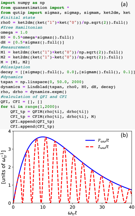
Figure 2: (a) The demonstrating code for the calculation of QFI and CFI with QuanEstimation. (b) The evolution of $\mathcal{F}_{\omega\omega}/t$ (solid blue line) and $\mathcal{I}_{\omega\omega}/t$ (dashed red line). The initial state is $|+\rangle$. The true value of $\omega$ ($\omega_{\mathrm{tr}}$) is set to be $1$, and the decay rates are set to be $\gamma_{+}/\omega_{\mathrm{tr}}=0$ and $\gamma_{-}/\omega_{\mathrm{tr}}=0.1$. Planck units are applied here.

In both functions QFIM() and CFIM(), the outputs are real numbers ($\mathcal{F}_{aa}$ and $\mathcal{I}_{aa}$) in the single-parameter case, namely, when drho only contains one entry, and they are real symmetric or Hermitian matrices in the multi-parameter scenarios. The basis of QFIM and CFIM are determined by the order of entries in drho. For example, when drho is $[\partial_{0}\rho,\partial_{1}\rho,\dots]$, the basis of the QFIM and CFIM is $\{x_{0},x_{1},\dots\}$.

For some specific scenarios, the calculation method in QFIM() may be not efficient enough. Therefore, we also provide the calculation of QFIM in some specific scenarios. The first one is the calculation in the Bloch representation. In this case, the function for the calculation of QFIM is of the form

⬇

QFIM_Bloch(r,dr,eps=1e-8)

The input r is an array representing a Bloch vector and dr is a list of arrays representing the derivatives of the Bloch vector on $\mathbb{x}$. Gaussian states are very commonly used in quantum metrology, and the corresponding QFIM can be calculated by the function:

⬇

QFIM_Gauss(R,dR,D,dD)

The input R is an array representing the first-order moment, i.e., the expected value $\langle\mathbb{R}\rangle:=\mathrm{Tr}(\rho\mathbb{R})$ of the vector $\mathbb{R}=(q_{1},p_{1},q_{2},p_{2},\dots)^{\mathrm{T}}$, where $q_{i}=(a_{i}+a^{\dagger}_{i})/\sqrt{2}$ and $p_{i}=(a_{i}-a^{\dagger}_{i})/(i\sqrt{2})$ are the quadrature operators with $a_{i}$ ($a^{\dagger}_{i}$) the annihilation (creation) operator of $i$th bosonic mode. dR is a list with $i$th entry also a list containing the derivatives $\partial_{\mathbb{x}}\langle[\mathbb{R}]_{i}\rangle$. Here $[\cdot]_{i}$ represents the $i$th entry of the vector. D is a matrix representing the second-order moment, $D_{ij}=\langle[\mathbb{R}]_{i}[\mathbb{R}]_{j}+[\mathbb{R}]_{j}[\mathbb{R}]_{i}\rangle/2$, and dD is a list of matrices representing the derivatives $\partial_{\mathbb{x}}D$. Notice that QFIM_Bloch() and QFIM_Gauss() can only compute the SLD-based QFIM.

Example. Now we present an example to show the usage of these functions. Consider a single qubit Hamiltonian $H=\omega\sigma_{3}/2$ with $\sigma_{3}$ a Pauli matrix and $\omega$ the frequency. Take $\omega$ as the parameter to be estimated and assume its true value (denoted by $\omega_{\mathrm{tr}}$) is 1. Planck unit ($\hbar=1$) is applied in the Hamiltonian. The dynamics is governed by the master equation

$$\partial_{t}\rho = -i\left[H,\rho\right]+\gamma_{+}\left(\sigma_{+}\rho\sigma_{-}-\frac{1}{2}\left\{\sigma_{-}\sigma_{+},\rho\right\}\right)$$ (12)

$$+\gamma_{-}\left(\sigma_{-}\rho\sigma_{+}-\frac{1}{2}\left\{\sigma_{+}\sigma_{-},\rho\right\}\right),$$

where $\sigma_{\pm}=(\sigma_{1}\pm\sigma_{2})/2$ with $\sigma_{1}$, $\sigma_{2}$ also Pauli matrices. $\gamma_{+}$ and $\gamma_{-}$ are the decay rates. The measurement is taken as $\{|+\rangle\langle+|,|-\rangle\langle-|\}$ with

$$|\pm\rangle:=\frac{1}{\sqrt{2}}(|0\rangle\pm|1\rangle).$$ (13)

Here $|0\rangle$ ($|1\rangle$) is the eigenstate of $\sigma_{3}$ with respect to the eigenvalue $1$ ($-1$). The specific code for the calculation of QFI/CFI are given in Fig. 2(a), and the corresponding evolution of $\mathcal{F}_{\omega\omega}/t$ (solid blue line) and $\mathcal{I}_{\omega\omega}/t$ (dashed red line) are shown in Fig. 2(b). The operators such as the density matrix and measurement can either be generated via QuTiP as in the demonstrating code or direct input.

IV.2 Holevo Cramér-Rao bound

Figure 3: Time evolution of $\mathrm{Tr}(W\mathcal{F}^{-1})$ (solid red line), $\mathrm{Tr}(W\mathcal{I}^{-1})$ (dashed black line), HCRB (dash-dotted blue line), and NHB (dotted green line) in the case of two-qubit system with the XX coupling. The probe state is $(|00\rangle+|11\rangle)/\sqrt{2}$. $W=\openone$ and $\omega_{1}=1$. The true values of $\omega_{2}$ and $g$ are $1$ and $0.1$, respectively. The decay rates $\gamma_{1}=\gamma_{2}=0.05\omega_{1}$. The POVM for $\mathrm{Tr}(W\mathcal{I}^{-1})$ is $\{\Pi_{1}$, $\Pi_{2}$, $\openone-\Pi_{1}-\Pi_{2}\}$ with $\Pi_{1}=0.85|00\rangle\langle 00|$ and $\Pi_{2}=0.4|\!+\!+\rangle\langle+\!+\!|$. Planck units are applied here.

Holevo Cramér-Rao bound (HCRB) is another useful asymptotic bound in quantum parameter estimation and tighter than the quantum Cramér-Rao bound in general. The HCRB can be expressed as [35, 14, 37, 36]

$$\mathrm{Tr}(W\mathrm{cov}(\hat{\mathbb{x}},\{\Pi_{y}\}))\geq\min_{\mathbb{X},V}\mathrm{Tr}(WV)$$ (14)

with $W$ the weight matrix and $V$ a matrix satisfying $V\geq Z(\mathbb{X})$. Here $Z(\mathbb{X})$ is a Hermitian matrix and its $ab$th entry is defined by $[Z(\mathbb{X})]_{ab}:=\mathrm{Tr}(\rho X_{a}X_{b})$, where $\mathbb{X}=[X_{0},X_{1},\cdots]$ is a vector of operators and its $a$th entry is defined by $X_{a}:=\sum_{y}(\hat{x}_{a}-x_{a})\Pi_{y}$ with $\hat{x}_{a}$ the $a$th entry of $\hat{\mathbb{x}}$. To let the local estimator $\hat{\mathbb{x}}$ unbiased, $\mathbb{X}$ needs to satisfy $\mathrm{Tr}(X_{a}\partial_{b}\rho)=\delta_{ab},\,\forall a,b$. Here $\delta_{ab}$ is the Kronecker delta function. An equivalent formulation of HCRB is [35, 14, 37, 36]

$$\min_{\mathbb{X},V}\mathrm{Tr}(WV)\!=\!\min_{\mathbb{X}}\leavevmode\nobreak\ \!\mathrm{Tr}(W\mathrm{Re}(Z))\!+\!\|\sqrt{W}\mathrm{Im}(Z)\sqrt{W}\|,$$ (15)

where $\mathrm{Re}(Z)$ and $\mathrm{Im}(Z)$ represent the real and imaginary parts of $Z$, and $\|\cdot\|$ is the trace norm, i.e., $\|A\|:=\mathrm{Tr}\sqrt{A^{\dagger}A}$ for a matrix $A$. Numerically, in a specific matrix basis $\{\lambda_{i}\}$ which satisfies $\mathrm{Tr}(\lambda_{i}\lambda_{j})=\delta_{ij}$, the HCRB can be solved via the semidefinite programming as it can be reformulated into a linear semidefinite problem [38],

$$\min_{\mathbb{X},V}\leavevmode\nobreak\ \mathrm{Tr}(WV),$$

$$\mathrm{subject}\leavevmode\nobreak\ \mathrm{to}\leavevmode\nobreak\ \begin{cases}\left(\begin{array}[]{cc}V&\Lambda^{\mathrm{T}}R^{\dagger}\\ R\Lambda&\openone\\ \end{array}\right)\geq 0,\\ \sum_{i}[\Lambda]_{ai}\mathrm{Tr}(\lambda_{i}\partial_{b}\rho)=\delta_{ab}.\end{cases}$$ (16)

Here the $ij$th entry of $\Lambda$ is obtained by decomposing $\mathbb{X}$ in the basis $\{\lambda_{i}\}$, $X_{i}=\sum_{j}[\Lambda]_{ij}\lambda_{j}$, and $R$ satisfies $Z=\Lambda^{\mathrm{T}}R^{\dagger}R\Lambda$. The semidefinite programming can be solved by the package CVXPY [39, 40] in Python and Convex [41] in Julia. In QuanEstimation, the HCRB can be calculated via the function:

⬇

HCRB(rho,drho,W,eps=1e-8)

The input W is the weight matrix and rho, drho have been introduced previously. Since $Z_{aa}$ is equivalent to the variance of the unbiased observable $O:=\sum_{y}\hat{x}_{a}\Pi_{y}$ [unbiased condition is $\mathrm{Tr}(\rho O)=x$], i.e., $Z_{aa}=\mathrm{Tr}(\rho O^{2})-[\mathrm{Tr}(\rho O)]^{2}$, in the case of single-parameter estimation the optimal $V$ is nothing but $Z_{aa}$ itself. Furthermore, it can be proved that $Z_{aa}\geq 1/\mathcal{F}_{aa}$ and the equality is attainable asymptotically. Hence, one can see that $\min_{X_{a}}Z_{aa}=1/\mathcal{F}_{aa}$, which means the HCRB is equivalent to the quantum Cramér-Rao bound in the single-parameter estimation. Due to better numerical efficiency of QFI computation, whenever drho has only one entry, the calling of HCRB() will automatically jump to QFIM() in the package. Similarly, if $W$ is a rank-one matrix, the HCRB also reduces to $\mathrm{Tr}(W\mathcal{F}^{-1})$ and thus in this case the calculation of HCRB will also be replaced by the calculation of QFIM.

Example. Now let us take a two-parameter estimation as an example to demonstrate the calculation of HCRB with QuanEstimation. Consider a two-qubit system with the XX coupling. The Hamiltonian of this system is

$$H=\omega_{1}\sigma^{(1)}_{3}+\omega_{2}\sigma^{(2)}_{3}+g\sigma^{(1)}_{1}\sigma^{(2)}_{1},$$ (17)

where $\omega_{1}$, $\omega_{2}$ are the frequencies of the first and second qubit, $\sigma^{(1)}_{i}=\sigma_{i}\otimes\openone$, and $\sigma^{(2)}_{i}=\openone\otimes\sigma_{i}$ for $i=1,2,3$. $\openone$ is the identity matrix. Planck units are applied here ($\hbar=1$). The parameters $\omega_{2}$ and $g$ are the ones to be estimated. The dynamics is governed by the master equation

$$\partial_{t}\rho=-i\left[H,\rho\right]+\sum_{i=1,2}\gamma_{i}\left(\sigma_{3}^{(i)}\rho\sigma_{3}^{(i)}-\rho\right)$$ (18)

with $\gamma_{i}$ the decay rate for $i$th qubit. The time evolutions of quantum Cramér-Rao bound [$\mathrm{Tr}(W\mathcal{F}^{-1})$], classical Cramér-Rao bound [$\mathrm{Tr}(W\mathcal{I}^{-1})$], and HCRB are shown in Fig. 3. The POVM for $\mathrm{Tr}(W\mathcal{I}^{-1})$ is $\{\Pi_{1}$, $\Pi_{2}$, $\openone-\Pi_{1}-\Pi_{2}\}$ with $\Pi_{1}=0.85|00\rangle\langle 00|$ and $\Pi_{2}=0.4|\!++\rangle\langle++\!|$. The probe state is $(|00\rangle+|11\rangle)/\sqrt{2}$ and the weight matrix $W=\openone$. As shown in this plot, HCRB (dash-dotted blue line) is tighter than $\mathrm{Tr}(W\mathcal{F}^{-1})$ (solid red line), which is in agreement with the fact that the HCRB is in general tighter than the quantum Cramér-Rao bound, unless the quantum Cramér-Rao bound is attainable, in which case the two bounds coincide [14].

IV.3 Nagaoka-Hayashi bound

Apart from the HCRB, the Nagaoka-Hayashi bound (NHB) [37, 42, 43] is another available bound for quantum multiparameter estimation, and is tighter than the HCRB in general. The expression of the NHB is

$$\mathrm{Tr}(W\mathrm{cov}(\hat{\mathbb{x}},\{\Pi_{y}\}))\geq\min_{\mathbb{X},\mathcal{Q}}\mathrm{Tr}\left((W\otimes\rho)\mathcal{Q}\right).$$ (19)

Here $\mathcal{Q}$ is a symmetric block matrix with each block a Hermitian matrix, and it satisfies $\mathcal{Q}\geq\mathbb{X}^{\mathrm{T}}\mathbb{X}$ with $\mathbb{X}$ defined in Sec. IV.2, namely, $\mathbb{X}=[X_{0},X_{1},\cdots]$ and $X_{a}=\sum_{y}(\hat{x}_{a}-x_{a})\Pi_{y}$. Similar to the HCRB, the calculation of NHB can also be reformulated into a linear semidefinite problem [43] as follows:

$$\min_{\mathbb{X},\mathcal{Q}}\leavevmode\nobreak\ \mathrm{Tr}\left((W\otimes\rho)\mathcal{Q}\right),$$

$$\mathrm{subject}\leavevmode\nobreak\ \mathrm{to}\leavevmode\nobreak\ \begin{cases}\left(\begin{array}[]{cc}\mathcal{Q}&\mathbb{X}^{\mathrm{T}}\\ \mathbb{X}&\openone\\ \end{array}\right)\geq 0,\\ \mathrm{Tr}(\rho X_{a})=0,\,\forall a,\\ \mathrm{Tr}(X_{a}\partial_{b}\rho)=\delta_{ab},\,\forall a,b.\\ \end{cases}$$ (20)

In QuanEstimation, the NHB can be calculated via the function:

⬇

NHB(rho,drho,W)

The performance of the NHB is also demonstrated in Fig. 3 with the Hamiltonian in Eq. (17) and dynamics in Eq. (18). In this case the NHB (dotted green line) is indeed slightly tighter than the HCRB, and thus also tighter than the quantum Cramér-Rao bound [$\mathrm{Tr}(W\mathcal{F}^{-1})$]. However, there still exist a gap between the classical Cramér-Rao bound [$\mathrm{Tr}(W\mathcal{I}^{-1})$] and the NHB, indicating that the chosen measurement may not be an optimal one.

IV.4 Bayesian estimation

Bayesian estimation is another well-used method in parameter estimation, in which the prior distribution is updated via the posterior distribution obtained by the Bayes’ rule

$$p(\mathbb{x}|y)=\frac{p(y|\mathbb{x})p(\mathbb{x})}{\int p(y|\mathbb{x})p(\mathbb{x})\mathrm{d}\mathbb{x}},$$ (21)

where $p(\mathbb{x})$ is the current prior distribution, $y$ is the result obtained in practice, and $\int\mathrm{d}\mathbb{x}:=\int\mathrm{d}x_{0}\int\mathrm{d}x_{1}\cdots$. The prior distribution is then updated with $p(\mathbb{x}|y)$, and the estimated value of $\mathbb{x}$ is obtained via a reasonable estimator, such as the expected value $\hat{\mathbb{x}}=\int\mathbb{x}p(\mathbb{x}|y)\mathrm{d}\mathbb{x}$ or the maximum a posteriori estimation (MAP), $\hat{\mathbb{x}}=\mathrm{argmax}_{\mathbb{x}}\,p(\mathbb{x}|y)$.

In QuanEstimation, the Bayesian estimation can be performed via the function:

⬇

pout,xout = Bayes(x,p,rho,y,M=[],

estimator="mean",savefile=False)

The input x is a list of arrays representing the regimes of $\mathbb{x}$, which is the same with the function BayesInput() discussed in Sec. III. Notice that in the package all the calculations of the integrals over the prior distributions are performed discretely. Hence, for now the input prior distribution is required to be an array, instead of a continuous function. p is an array representing the values of $p(\mathbb{x})$ with respect to $\mathbb{x}$. It is multidimensional in the case of multiparameter estimation, i.e., the entry number of x are at least two. The input rho is a (multidimensional) list of matrices representing the values of density matrix with respect to all values of $\mathbb{x}$, which can be alternatively generated via the function BayesInput() if specific functions of $H$ and $\partial_{\mathbb{x}}H$ on $\mathbb{x}$ can be provided. M=[] is a list of matrices representing a set of POVM and its default setting is a SIC-POVM. y is an array representing the results obtained in an experiment. The result corresponds to the POVM operator input in M, which means it is an integer between 0 and $d-1$ with $d$ the entry number of the set of POVM. The type of estimator can be set via estimator=" " and currently it has two choices. When estimator="mean" the estimator is the expected value, and when estimator="MAP" the estimator is the MAP. The output pout (a multidimensional array) and xout (an array) are the final posterior distribution and estimated value of $\mathbb{x}$ obtained via the chosen estimator. When savefile=True, two files "pout.npy" and "xout.npy" will be generated, which include the updated $p(\mathbb{x})$ and the corresponding optimal $\mathbb{x}$ in all rounds. If the users call this function in the full-Julia package, the output files are "pout.csv" and "xout.csv".

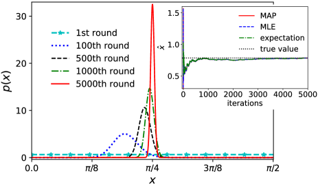
Figure 4: Iteration of posterior distribution by the Bayes’ rule. The inset shows the change of estimated value as a function of iteration for MAP (solid red line), MLE (dashed blue line), and expectation (dash-dotted green line). The dotted black line represents the true value.

Example. Now let us consider a simple example with the Hamiltonian

$$H=\frac{\kappa\omega_{0}}{2}(\sigma_{1}\cos x+\sigma_{3}\sin x),$$ (22)

where $x$, $\kappa$ are two dimensionless parameters and $x$ is taken as the unknown one. Planck units are applied here ($\hbar=1$) and $\omega_{0}$ is set to be 1. The initial state is taken as $|+\rangle$ and the target time $\omega_{0}T=1$. The prior distribution is assumed to be uniform in the regime $[0,\pi/2]$. The measurement is $\{|+\rangle\langle+|,|-\rangle\langle-|\}$. The results in experiment are simulated by a random generation according to the probabilities $p(\pm|x)=\langle\pm|\rho|\pm\rangle$ with respect to the value $x=\pi/4$. As shown in Fig. 4, with the growth of iteration number, the deviation decreases monotonously and the estimated value (center value of the distribution) approaches to $\pi/4$, which can also be confirmed by the convergence of estimated value (solid red line) shown in the inset. As a matter of fact, here the maximum likelihood estimation (MLE) can also provide similar performance by taking the likelihood function with the MAP estimator $\hat{\mathbb{x}}=\mathrm{argmax}_{\mathbb{x}}\,\prod_{i}p(y_{i}|\mathbb{x})$ (dashed blue line in the inset). In QuanEstimation, this MLE can be calculated by the function:

⬇

Lout,xout = MLE(x,rho,y,M=[],savefile=False)

When savefile=True, two files "Lout.npy" and "xout.npy" will be generated including all the data in the iterations.

In Bayesian estimation, another useful tool is the average Bayesian cost [44] for the quadratic cost, which is defined by

$$\bar{C}:=\int p(\mathbb{x})\sum_{y}p(y|\mathbb{x})(\mathbb{x}-\hat{\mathbb{x}})^{\mathrm{T}}W(\mathbb{x}-\hat{\mathbb{x}})\,\mathrm{d}\mathbb{x}$$ (23)

with $W$ the weight matrix. In QuanEstimation, this average Bayesian cost can be calculated via the function:

⬇

BayesCost(x,p,xest,rho,M,W=[],eps=1e-8)

Here x and p are the same with those in Bayes(). xest is a list of arrays representing the estimator $\hat{\mathbb{x}}$. The $i$th entry of each array in xest represents the estimator with respect to $i$th result. In the case of the single-parameter scenario, $W$ is chosen to be 1 regardless of the input. The average Bayesian cost satisfies the inequality [14]

$$\bar{C}\geq\int p(\mathbb{x})\left(\mathbb{x}^{\mathrm{T}}W\mathbb{x}\right)\mathrm{d}\mathbb{x}-\sum_{ab}W_{ab}\mathrm{Tr}\left(\bar{\rho}\bar{L}_{a}\bar{L}_{b}\right),$$ (24)

where $\bar{\rho}:=\int p(\mathbb{x})\rho\,\mathrm{d}\mathbb{x}$ and the operator $\bar{L}_{a}$ is determined by the equation $\int x_{a}p(\mathbb{x})\rho\,\mathrm{d}\mathbb{x}=(\bar{L}_{a}\bar{\rho}+\bar{\rho}\bar{L}_{a})/2$. In the case of the single-parameter scenario, the inequality above reduces to

$$\bar{C}\geq\int p(x)x^{2}\,\mathrm{d}x-\mathrm{Tr}(\bar{\rho}\bar{L}^{2})$$ (25)

and represents a bound which is always saturable—the optimal measurement correspond to projection measurement in the eigenbasis of $\bar{L}$, while the corresponding eigenvalues represent the estimated values of the parameter. If the mean value $\int p(x)x\,\mathrm{d}x$ is subtracted to zero, then the inequality above can be rewritten into $\bar{C}\geq\delta^{2}x-\mathrm{Tr}(\bar{\rho}\bar{L}^{2})$ with $\delta^{2}x:=\int p(x)x^{2}\,\mathrm{d}x-\int p(x)x\,\mathrm{d}x$ the variance of $x$ under the prior distribution. In QuanEstimation, the bound given in Eq. (24) can be calculated via the following function:

⬇

BCB(x,p,rho,W=[],eps=1e-8)

Here the inputs x and p are the some with those in Bayes() and BayesCost(). W represents the weight matrix and the default value is the identity matrix.

IV.5 Bayesian Cramér-Rao bounds

In the Bayesian scenarios, the quantum Cramér-Rao Bounds and Holevo Cramér-Rao bound are not appropriate to grasp the the ultimate precision limits as they are ignorant of the prior information. Still, Bayesian Cramér-Rao bounds can be used instead. In these scenarios, the covariance matrix is redefined as

$$\mathrm{cov}(\hat{\mathbb{x}},\{\Pi_{y}\})\!=\!\int\!p(\mathbb{x})\sum_{y}\mathrm{Tr}(\rho\Pi_{y})(\hat{\mathbb{x}}\!-\!\mathbb{x})(\hat{\mathbb{x}}\!-\!\mathbb{x})^{\mathrm{T}}\mathrm{d}\mathbb{x},$$ (26)

where the integral $\int\mathrm{d}\mathbb{x}:=\iiint\mathrm{d}x_{0}\mathrm{d}x_{1}\cdots$. In such cases, one version of the Bayesian Cramér-Rao bound (BCRB) is of the form

$$\mathrm{cov}(\hat{\mathbb{x}},\{\Pi_{y}\})\geq\int p(\mathbb{x})\left(B\mathcal{I}^{-1}B+\mathbb{b}\mathbb{b}^{\mathrm{T}}\right)\mathrm{d}\mathbb{x},$$ (27)

where $\mathcal{I}$ is the CFIM, and $\mathbb{b}=(b(x_{0}),b(x_{1}),\dots)^{\mathrm{T}}$ is the vector of biases, i.e., $b(x_{a})=\sum_{y}\hat{x}_{a}p(y|\mathbb{x})-x_{a}$ for each $x_{a}$ with $p(y|\mathbb{x})$ the conditional probability. $B$ is a diagonal matrix with the $a$th entry $B_{aa}=1+[\mathbb{b}^{\prime}]_{a}$. Here $\mathbb{b}^{\prime}:=(\partial_{0}b(x_{0}),\partial_{1}b(x_{1}),\dots)^{\mathrm{T}}$. The quantum correspondence of this bound (BQCRB) reads

$$\mathrm{cov}(\hat{\mathbb{x}},\{\Pi_{y}\})\geq\int p(\mathbb{x})\left(B\mathcal{F}^{-1}B+\mathbb{b}\mathbb{b}^{\mathrm{T}}\right)\mathrm{d}\mathbb{x},$$ (28)

where $\mathcal{F}$ is the QFIM of all types. As a matter of fact, there exists a similar version of Eq. (27), which can be expressed by

$$\mathrm{cov}(\hat{\mathbb{x}},\{\Pi_{y}\})\geq\mathcal{B}\,\mathcal{I}_{\mathrm{Bayes}}^{-1}\,\mathcal{B}+\int p(\mathbb{x})\mathbb{b}\mathbb{b}^{\mathrm{T}}\mathrm{d}\mathbb{x},$$ (29)

where $\mathcal{I}_{\mathrm{Bayes}}=\int p(\mathbb{x})\mathcal{I}\mathrm{d}\mathbb{x}$ is the average CFIM with $\mathcal{I}$ the CFIM defined in Eq. (6). $\mathcal{B}=\int p(\mathbb{x})B\mathrm{d}\mathbb{x}$ is the average of $B$. Its quantum correspondence reads

$$\mathrm{cov}(\hat{\mathbb{x}},\{\Pi_{y}\})\geq\mathcal{B}\,\mathcal{F}_{\mathrm{Bayes}}^{-1}\,\mathcal{B}+\int p(\mathbb{x})\mathbb{b}\mathbb{b}^{\mathrm{T}}\mathrm{d}\mathbb{x},$$ (30)

where $\mathcal{F}_{\mathrm{Bayes}}=\int p(\mathbb{x})\mathcal{F}\mathrm{d}\mathbb{x}$ is average QFIM with $\mathcal{F}$ the QFIM of all types.

Another version of the Bayesian Cramér-Rao bound is of the form

$$\mathrm{cov}(\hat{\mathbb{x}},\{\Pi_{y}\})\geq\int p(\mathbb{x})\mathcal{G}\left(\mathcal{I}_{p}+\mathcal{I}\right)^{-1}\mathcal{G}^{\mathrm{T}}\mathrm{d}\mathbb{x},$$ (31)

and its quantum correspondence can be expressed by

$$\mathrm{cov}(\hat{\mathbb{x}},\{\Pi_{y}\})\geq\int p(\mathbb{x})\mathcal{G}\left(\mathcal{I}_{p}+\mathcal{F}\right)^{-1}\mathcal{G}^{\mathrm{T}}\mathrm{d}\mathbb{x},$$ (32)

where the entries of $\mathcal{I}_{p}$ and $\mathcal{G}$ are defined by

$$[\mathcal{I}_{p}]_{ab}:=[\partial_{a}\ln p(\mathbb{x})][\partial_{b}\ln p(\mathbb{x})],$$ (33)

and $\mathcal{G}_{ab}:=[\partial_{b}\ln p(\mathbb{x})][\mathbb{b}]_{a}+B_{aa}\delta_{ab}$. The derivations and thorough discussions of these bounds will be further discussed in an independent paper, which will be announced in a short time.

The functions in QuanEstimation to calculate $\mathcal{I}_{\mathrm{Bayes}}$ and $\mathcal{F}_{\mathrm{Bayes}}$ are:

⬇

BCFIM(x,p,rho,drho,M=[],eps=1e-8)

BQFIM(x,p,rho,drho,LDtype="SLD",eps=1e-8)

And the functions for the calculations of BCRBs and BQCRBs are:

⬇

BCRB(x,p,dp,rho,drho,M=[],b=[],db=[],

btype=1,eps=1e-8)

BQCRB(x,p,dp,rho,drho,b=[],db=[],btype=1,

LDtype="SLD",eps=1e-8)

The input x and p are the same with those in the function Bayes(). dp is a (multidimensional) list of arrays representing the derivatives of the prior distribution, which is only essential when btype=3. In the case that btype=1 and btype=2, it could be set as []. rho and drho are (multidimensional) lists representing the values of $\rho$ and $\partial_{\mathbb{x}}\rho$. For example, if the input x includes three arrays, which are the values of $x_{0}$, $x_{1}$, and $x_{2}$ for the integral, then the $ijk$th entry of rho and drho are a matrix $\rho$ and a list $[\partial_{0}\rho,\partial_{1}\rho,\partial_{2}\rho]$ with respect to the values $[x_{0}]_{i}$, $[x_{1}]_{j}$, and $[x_{2}]_{k}$. Here $[x_{0}]_{i}$, $[x_{1}]_{j}$, and $[x_{2}]_{k}$ represent the $i$th, $j$th, and $k$th value in the first, second, and third array in x. As a matter of fact, if the users can provide specific functions of $H$ and $\partial_{\mathbb{x}}H$ on $\mathbb{x}$, rho and drho can be alternatively generated via the functions BayesInput() and Lindblad() [or Kraus()]. b and db are two lists of arrays representing $\mathbb{b}$ and $\mathbb{b}^{\prime}$, and the default settings for both of them are zero vectors (unbiased). In BCRB() the measurement is input via M=[], and if it is empty, a set of rank-one SIC-POVM will be automatically applied, similar to that in CFIM(). Moreover, btype=1, btype=2, and btype=3 represent the calculation of Eqs. (27), (29), and (31). In the meantime, in BQCRB(), btype=1, btype=2, and btype=3 represent the calculation of Eqs. (28), (30) and (32). Similar to QFIM(), LDtype=" " here is the type of logarithmic derivatives, including three choices: "SLD", "RLD", and "LLD". Recently, Ref. [45] provide an optimal biased bound based on the type-1 BQCRB in the case of single-parameter estimation, which can be calculated in QuanEstimation via the function:

⬇

OBB(x,p,dp,rho,drho,d2rho,LDtype="SLD",

eps=1e-8)

The input dp is an array containing the derivatives $\partial_{x}p$. d2rho is a list containing the second order derivative of the density matrix on the unknown parameter.

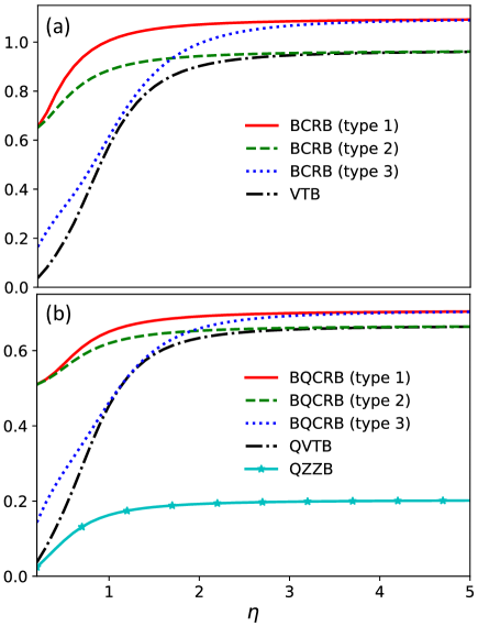
Figure 5: (a) The performance of classical Bayesian bounds, including BCRB of type 1 (solid red line), type 2 (dashed green line), type 3 (dotted blue line), and VTB (dash-dotted black line). (b) The performance of quantum Bayesian bounds, including BQCRB of type 1 (solid red line), type 2 (dashed green line), type 3 (dotted blue line), QVTB (dash-dotted black line), and QZZB (solid cyan pentagram line). The parameters $\mu=0$ and $\kappa=\pi/2$ in the plots. Planck units are applied here.

Another famous Bayesian version of Cramér-Rao bound is introduced by Van Trees in 1968 [46], which is known as the Van Trees bound (VTB). The VTB is expressed by

$$\mathrm{cov}(\hat{\mathbb{x}},\{\Pi_{y}\})\geq\left(\mathcal{I}_{\mathrm{prior}}+\mathcal{I}_{\mathrm{Bayes}}\right)^{-1},$$ (34)

where $\mathcal{I}_{\mathrm{prior}}=\int p(\mathbb{x})\mathcal{I}_{p}\mathrm{d}\mathbb{x}$ is the CFIM for $p(\mathbb{x})$ with $\mathcal{I}_{p}$ defined in Eq. (33). In the derivation, the assumption

$$\int\partial_{a}\left[b(x_{b})p(\mathbb{x})\right]\mathrm{d}\mathbb{x}=0$$ (35)

is applied for all subscripts $a$ and $b$. In 2011, Tsang, Wiseman and Caves [47] provided a quantum correspondence of the VTB (QVTB). The Tsang-Wiseman-Caves bound is of the form

$$\mathrm{cov}(\hat{\mathbb{x}},\{\Pi_{y}\})\geq\left(\mathcal{I}_{\mathrm{prior}}+\mathcal{F}_{\mathrm{Bayes}}\right)^{-1}.$$ (36)

The functions in QuanEstimation for the calculation of VTB and QVTB are:

⬇

VTB(x,p,dp,rho,drho,M=[],eps=1e-8)

QVTB(x,p,dp,rho,drho,LDtype="SLD",eps=1e-8)

Here dp is a (multidimensional) list of arrays representing the derivatives of the prior distribution. For example, if x includes 3 arrays, which are the values of $x_{0}$, $x_{1}$, and $x_{2}$ for the integral, then the $ijk$th entry of dp is an array $(\partial_{0}p,\partial_{1}p,\partial_{2}p)$ with respect to values $[x_{0}]_{i}$, $[x_{1}]_{j}$ and $[x_{2}]_{k}$.

Example. Let us still take the Hamiltonian in Eq. (22) and initial state $|+\rangle$ as an example. $x$ is still the parameter to be estimated. The prior distribution is taken as a Gaussian distribution

$$p(x)=\frac{1}{c\eta\sqrt{2\pi}}e^{-\frac{(x-\mu)^{2}}{2\eta^{2}}}$$ (37)

in a finite regime $[-\pi/2,\pi/2]$, where $\mu$ is the expectation, $\eta$ is the standard deviation, and $c=\frac{1}{2}\big{[}\mathrm{erf}(\frac{\pi-2\mu}{2\sqrt{2}\eta})+\mathrm{erf}(\frac{\pi+2\mu}{2\sqrt{2}\eta})\big{]}$ is the normalized coefficient. Here $\mathrm{erf}(x):=\frac{2}{\sqrt{\pi}}\int^{x}_{0}e^{-t^{2}}\mathrm{d}t$ is the error function. The measurement in the classical bounds is taken as a set of SIC-POVM. The performance of the classical and quantum Bayesian bounds are given in Figs. 5(a) and 5(b). As shown in Fig. 5(a), in this case BCRB of type 1 (solid red line) and type 2 (dashed green line) are tighter than type 3 (dotted blue line) and VTB (dash-dotted black line) when the deviation $\eta$ is small. With the increase of $\eta$, BCRB of type 1 and type 3 coincide with each other, so do BCRB of type 2 and VTB. Furthermore, BCRB of type 1 and type 3 are always tighter than type 2 and VTB in this example. The performance of quantum Bayesian bounds are similar, as shown in Fig. 5(b). BQCRB (solid red line for type 1 and dashed green line for type 2) are tighter than type 3 (dotted green line) and QVTB (dash-dotted black line) when $\eta$ is small and BQCRB of type 1 (type 2) and type 3 (QVTB) coincide with each other for a large $\eta$.

IV.6 Quantum Ziv-Zakai bound

Apart from the Cramér-Rao bounds, the Ziv-Zakai bound is another useful bound in Bayesian scenarios. It was first provided by Ziv and Zakai in 1969 [48] for the single-parameter estimation and then extended to the linear combination of multiple parameters by Bell et al. [49], which is also referred to as the Bell-Ziv-Zakai bound. In 2012, Tsang provided a quantum correspondence of the Ziv-Zakai bound [50] (QZZB), and in 2015 Berry et al. [51] provided a quantum correspondence of the Bell-Ziv-Zakai bound. In QZZB, the variance $\mathrm{var}(\hat{x},\{\Pi_{y}\})$, a diagonal entry of the covariance matrix, satisfies the following inequality

$$\mathrm{var}(\hat{x},\{\Pi_{y}\}) \geq \frac{1}{2}\int_{0}^{\infty}\mathrm{d}\tau\tau\mathcal{V}\int_{-\infty}^{\infty}\mathrm{d}x\min\!\left\{p(x),p(x+\tau)\right\}$$ (38)

$$\times\left(1-\frac{1}{2}||\rho(x)-\rho(x+\tau)||\right),$$

where $||\cdot||$ is the trace norm. $\mathcal{V}$ is the "valley-filling" operator satisfying $\mathcal{V}f(\tau)=\max_{h\geq 0}f(\tau+h)$. In the numerical calculations, the prior distribution has to be limited or truncated in a finite regime $[\alpha,\beta]$, i.e., $p(x)=0$ when $x>\beta$ or $x<\alpha$, and then the QZZB reduces to

$$\mathrm{var}(\hat{x},\{\Pi_{y}\}) \geq \frac{1}{2}\int_{0}^{\beta-\alpha}\mathrm{d}\tau\tau\mathcal{V}\int_{\alpha}^{\beta}\mathrm{d}x\min\left\{p(x),p(x+\tau)\right\}$$ (39)

$$\times\left(1-\frac{1}{2}||\rho(x)-\rho(x+\tau)||\right).$$

The function in QuanEstimation for the calculation of QZZB is:

⬇

QZZB(x,p,rho,eps=1e-8)

The performance of QZZB is also demonstrated with the Hamiltonian in Eq. (22) and prior distribution in Eq. (37), as shown in Fig. 5(b). In this example, its performance (solid cyan pentagram line) is worse than BQCRB and QVTB. However, this tightness relation may dramatically change in other systems or with other prior distributions. Hence, in a specific scenario using QuanEstimation to perform a thorough comparison would be a good choice to find the tightest tool for the scheme design.

V Metrological resources

The improvement of precision usually means a higher consumption of resources. For example, the repetition of experiments will make the deviation of the unknown parameter to scale proportionally to $1/\sqrt{n}$ ($n$ the repetition number) in theory. The repetition number or the total time is thus the resource responsible for this improvement. Constraint on quantum resources is an important aspect in the study of quantum parameter estimation, and is crucial to reveal the quantum advantage achievable in practical protocols. The numerical calculations of some typical resources have been added in QuTiP, such as various types of entropy and the concurrence. Hence, we do not need to rewrite them in QuanEstimation. Currently, two additional metrological resources, spin squeezing and the time to reach a given precision limit are provided in the package. The spin squeezing can be calculated via the function:

⬇

SpinSqueezing(rho,basis="Dicke",output="KU")

Here the input rho is a matrix representing the state. The basis of the state can be adjusted via basis=" ". Two options "Dicke" and "Pauli" represent the Dicke basis and the original basis of each spin. basis="Pauli" here is equivalent to choose basis="uncoupled" in the function jspin() in QuTiP. Two types of spin squeezing can be calculated in this function. output="KU" means the output is the one given by Kitagawa and Ueda [52], and output="WBIMH" means the output is the one given by Wineland et al. [53].

The time to reach a given precision limit can be calculated via the function:

⬇

TargetTime(f,tspan,func,*args,**kwargs)

Notice that the dynamics needs to be run first before using this function. For example, it is available to be called after the calling of both Lindblad() and Lindblad.expm(). The input f is a float number representing the given value of the precision limit. The time is searched within the regime defined by the input tspan (an array). func is the handle of a function func() depicting the precision limit. *args is the corresponding input parameters, in which rho and drho should be the output of Lindblad.expm() [or Lindblad.ode() and any other method that may included in the future]. **kwargs is the keyword arguments in func(). The difference between input parameters and keyword arguments in QuanEstimation is that the keyword arguments have default values and thus one does not have to assign values to them when calling the function. Currently, all the asymptotic bounds discussed in Sec. IV are available to be called here.

Algorithms	method=	**kwargs and default values
auto-GRAPE	"auto-GRAPE"	"Adam"	True
(GRAPE)	("GRAPE")	"ctrl0"	[]
		"max_episode"	300
		"epsilon"	0.01
		"beta1"	0.90
		"beta2"	0.99
PSO	"PSO"	"p_num"	10
		"ctrl0"	[]
		"max_episode"	[1000,100]
		"c0"	1.0
		"c1"	2.0
		"c2"	2.0
		"seed"	1234
DE	"DE"	"p_num"	10
		"ctrl0"	[]
		"max_episode"	1000
		"c"	1.0
		"cr"	0.5
		"seed"	1234
DDPG	"DDPG"	"ctrl0"	[]
		"max_episode"	500
		"layer_num"	3
		"layer_dim"	200
		"seed"	1234

Table 1: Available control methods in QuanEstimation andcorresponding default parameter settings. Notice that auto-GRAPE and GRAPE are not available when control.HCRB() is called.

VI Control optimization

Quantum control is a leading approach in quantum metrology to achieve the improvement of measurement precision and boost the resistance to decoherence. This is possible thanks to high controllability of typical quantum metrological setups. A paradigmatic controllable Hamiltonian is of the form

$$H=H_{0}(\mathbb{x})+\sum^{K}_{k=1}u_{k}(t)H_{k},$$ (40)

where $H_{0}(\mathbb{x})$ is the free Hamiltonian containing the unknown parameters $\mathbb{x}$ and $H_{k}$ is the $k$th control Hamiltonian with the corresponding control amplitude $u_{k}(t)$. In quantum parameter estimation, the aim of control is to improve the precision of the unknown parameters. Hence, natural choices for the the objective function $f$ are the various metrological bounds. The quantum Cramér-Rao bounds are easiest to calculate and hence will typically be the first choice. In the single-parameter estimation, the QFI or CFI can be taken as the objective function, depending whether the measurement can be optimized or is fixed. In the multiparameter scenario, the objective function can be $\mathrm{Tr}(W\mathcal{F}^{-1})$, $\mathrm{Tr}(W\mathcal{I}^{-1})$, or the HCRB.

Searching the optimal controls in order to achieve the maximum or minimum values of an objective function is the core task in quantum control. Most existing optimization algorithms, such as Gradient ascent pulse engineering [54, 55, 56], Krotov’s method [57, 58, 59], and machine learning [60, 61], are capable of providing useful control strategies in quantum parameter estimation. The gradient-based algorithms usually perform well in small-scale systems. For complex problems where the gradient-based methods are more challenging or even fail to work at all, gradient-free algorithms are a good alternative. Here we introduce several control algorithms in quantum parameter estimation that have been added into our package and give some illustrations.

First, we present the specific code in QuanEstimation for the execution of the control optimization,

⬇

control = ControlOpt(savefile=False,

method="auto-GRAPE",**kwargs)

control.dynamics(tspan,rho0,H0,dH,Hc,

decay=[],ctrl_bound=[],

dyn_method="expm")

control.QFIM(W=[],LDtype="SLD")

control.CFIM(M=[],W=[])

control.HCRB(W=[])

The input tspan is an array representing the time for the evolution. rho0 is a matrix representing the density matrix of the initial state. H0 is a matrix representing the free Hamiltonian $H_{0}(\mathbb{x})$ and Hc is a list containing the control Hamiltonians, i.e., $[H_{1},H_{2},\dots]$. dH is a list of matrices representing $\partial_{\mathbb{x}}H_{0}$. In the case that only one entry exists in dH, the objective functions in control.QFIM() and control.CFIM() are the QFI and CFI, and if more than one entries are input, the objective functions are $\mathrm{Tr}(W\mathcal{F}^{-1})$ and $\mathrm{Tr}(W\mathcal{I}^{-1})$. Different types of QFIM can be selected as the objective function via the variable LDtype=" ", which includes three options "SLD", "RLD", and "LLD". The measurement for CFI/CFIM is input via M=[] in control.CFIM() and the default value is a SIC-POVM. The weight matrix $W$ can be manually input via W=[], and the default value is the identity matrix.

In some cases, the control amplitudes have to be limited in a regime, for example $[a,b]$, which can be realized by input ctrl_bound=[a,b]. If no value is input, the default regime is $[-\infty,\infty]$. decay=[] is a list of decay operators and corresponding decay rates for the master equation in Eq. (1) and its input rule is decay=[[Gamma_1,gamma_1],…]. The dynamics is solved via the matrix exponential by default, which can be switched to ODE by setting dyn_method="ode". The default value for savefile is False, which means only the controls obtained in the final episode will be saved in the file named "controls.csv", and if it is set to be True, the controls obtained in all episodes will be saved in this file. The values of QFI, CFI, $\mathrm{Tr}(W\mathcal{F}^{-1})$ or $\mathrm{Tr}(W\mathcal{I}^{-1})$ in all episodes will be saved regardless of this setting in the file named "f.csv". Another file named "total_reward.csv" will also be saved to save the total rewards in all episodes when DDPG is chosen as the optimization method. Here the word "episode" is referred to as a round of update of the objective function in the scenario of optimization.

The switch of optimization algorithms can be realized by method=" ", and the corresponding parameters can be set via **kwargs. All available algorithms in QuanEstimation are given in Table 1 together with the corresponding default parameter settings. Notice that in the case that method="auto-GRAPE" is applied, dyn_method="ode" is not available for now. In some algorithms maybe more than one set of guessed controls are needed, and if not enough sets are input then random-value controls will be generated automatically to fit the number. In the meantime, if excessive number of sets are input, only the suitable number of controls will be used. LDtype="SLD" is the only choice when method="GRAPE" as the QFIMs based on RLD and LLD are unavailable to be the objective function for GRAPE in the package. All the aforementioned algorithms will be thoroughly introduced and discussed with examples in the following subsections.

Initialize the control amplitude $u_{k}(t)$ for all $t$ and $k$;

for episode=1, $M$ do

       Receive initial state $\rho_{0}$ ($\rho_{\mathrm{in}}$);

       for $t=1,T$ do

             Evolve with the control $\rho_{t}=e^{\Delta t\mathcal{L}_{t}}\rho_{t-1}$;

             Calculate the derivatives $\partial_{\mathbb{x}}\rho_{t}=-i\Delta t[\partial_{\mathbb{x}}H_{0}(\mathbb{x})]^{\times}\rho_{t}+e^{\Delta t\mathcal{L}_{t}}\partial_{\mathbb{x}}\rho_{t-1}$;

             Save $\rho_{t}$ and $\partial_{\mathbb{x}}\rho_{t}$;

             for $k=1,K$ do

                   Calculate $\frac{\delta\rho_{t}}{\delta u_{k}(t)}=-i\Delta tH^{\times}_{k}\rho_{t}$, $\partial_{\mathbb{x}}\!\left(\!\frac{\delta\rho_{t}}{\delta u_{k}(t)}\!\right)=-i\Delta tH^{\times}_{k}(\partial_{\mathbb{x}}\rho_{t})$;

                   for $j=t-1,1$ do

                         Calculate $\frac{\delta\rho_{t}}{\delta u_{k}(j)}=e^{\Delta t\mathcal{L}_{t}}\frac{\delta\rho_{t-1}}{\delta u_{k}(j)}$, $\partial_{\mathbb{x}}\!\left(\frac{\delta\rho_{t}}{\delta u_{k}(j)}\right)=\left(\partial_{\mathbb{x}}e^{\Delta t\mathcal{L}_{t}}\right)\frac{\delta\rho_{t-1}}{\delta u_{k}(j)}+e^{\Delta t\mathcal{L}_{t}}\partial_{\mathbb{x}}\!\left(\frac{\delta\rho_{t-1}}{\delta u_{k}(j)}\right)$;

                   end for

                  Save $\frac{\delta\rho_{t}}{\delta u_{k}(t)}$, $\partial_{\mathbb{x}}\!\left(\frac{\delta\rho_{t}}{\delta u_{k}(t)}\right)$ and all $\frac{\delta\rho_{t}}{\delta u_{k}(j)}$, $\partial_{\mathbb{x}}\!\left(\frac{\delta\rho_{t}}{\delta u_{k}(j)}\right)$;

             end for

            

       end for

      Calculate the SLDs for all $\mathbb{x}$ and the objective function $f(T)$;

       for $t=1,T$ do

             for $k=1,K$ do

                   Calculate the gradient $\frac{\delta f(T)}{\delta u_{k}(t)}$ with $\frac{\delta\rho_{T}}{\delta u_{k}(t)}$ and $\partial_{\mathbb{x}}\!\left(\frac{\delta\rho_{T}}{\delta u_{k}(t)}\right)$;

                   Update control $u_{k}(t)\!\leftarrow\!u_{k}(t)\!+\!\epsilon\frac{\delta f(T)}{\delta u_{k}(t)}$.

             end for

            

       end for

      

end for

Save the controls $\{u_{k}(t)\}$ and corresponding $f(T)$.

Algorithm 1 GRAPE

Apart from the QFIM and CFIM, the HCRB can also be taken as the objective function in the case of multiparameter estimation, which can be realized by calling control.HCRB(). Notice that auto-GRAPE and GRAPE are not available in method=" " here as the calculation of HCRB is performed via optimizations (semidefinite programming), not direct calculations. Due to the equivalence between the HCRB and quantum Cramér-Rao bound in the single-parameter estimation, if control.HCRB() is called in this case, the entire program will be terminated and a line of reminder will arise to remind the users to invoke control.QFIM() instead.

VI.1 Gradient ascent pulse engineering

The gradient ascent pulse engineering algorithm (GRAPE) was developed by Khaneja et al. [54] in 2005 for the design of pulse sequences in the Nuclear Magnetic Resonance systems, and then applied into the quantum parameter estimation for the generation of optimal controls [55, 56], in which the gradients of the objective function $f(T)$ at a fixed time $T$ were obtained analytically. In the pseudocode given in Ref. [17], the propagators between any two time points have to be saved, which would occupy a large amount of memory during the computation and make it difficult to deal with high-dimensional Hamiltonians or long-time evolutions. To solve this problem, a modified pseudocode is provided as given in Algorithm 1. In this modified version, after obtaining the evolved state $\rho_{t}$ and $\partial_{\mathbb{x}}\rho_{t}$, the gradient $\delta\rho_{t}/\delta u_{k}(t)$ and its derivatives with respect to $\mathbb{x}$ are then calculated via the equations

$$\frac{\delta\rho_{t}}{\delta u_{k}(t)}=-i\Delta tH^{\times}_{k}(\rho_{t})$$ (41)

with $\Delta t$ a small time interval, $H^{\times}_{k}(\cdot)=[H_{k},\cdot]$ the commutator between $H_{k}$ and other operators, and

$$\partial_{\mathbb{x}}\!\left(\frac{\delta\rho_{t}}{\delta u_{k}(t)}\!\right)=-i\Delta tH^{\times}_{k}(\partial_{\mathbb{x}}\rho_{t}),$$ (42)

The gradients $\delta\rho_{t}/\delta u_{k}(j)$ ($j<t$) are calculated adaptively according to the equation

$$\frac{\delta\rho_{t}}{\delta u_{k}(j)}=e^{\Delta t\mathcal{L}_{t}}\frac{\delta\rho_{t-1}}{\delta u_{k}(j)}$$ (43)

and its derivatives are obtained via

$$\partial_{\mathbb{x}}\!\left(\frac{\delta\rho_{t}}{\delta u_{k}(j)}\right)\!=\!\left(\partial_{\mathbb{x}}e^{\Delta t\mathcal{L}_{t}}\right)\!\frac{\delta\rho_{t-1}}{\delta u_{k}(j)}\!+\!e^{\Delta t\mathcal{L}_{t}}\partial_{\mathbb{x}}\!\left(\frac{\delta\rho_{t-1}}{\delta u_{k}(j)}\right)\!.$$ (44)

In this process, only the gradients $\delta\rho_{t}/\delta u_{k}(t)$, $\delta\rho_{t}/\delta u_{k}(j)$ and their derivatives need to be saved for the further use in the next round, and will be deleted after that. This operation avoids the usage of propagators and thus saves a lot of memory during the computation. In this way, the gradients $\delta\rho_{T}/\delta u_{k}(t)$ ($t$ is any time here) are obtained adaptively and $\delta f(T)/\delta u_{k}(t)$ can then be calculated accordingly. The specific expression of $\delta f(T)/\delta u_{k}(t)$ can be found in Refs. [55, 56, 13]. Adam [62] is also applied in this algorithm for the further improvement of the computational efficiency.

Consider the dynamics governed by Eq. (12) with parameter settings in Fig. 2, and the control Hamiltonian

$$u_{1}(t)\sigma_{1}+u_{2}(t)\sigma_{2}+u_{3}(t)\sigma_{3}.$$ (45)

In the case of $\omega_{\mathrm{tr}}T=5$ with zeros as the initial guess of the controls, the QFI converges in 35 rounds with Adam, yet it takes 780 rounds to converge when Adam is not applied.

VI.2 Auto-GRAPE

In the multiparameter estimation, the gradients of $\mathrm{Tr}(W\mathcal{F}^{-1})$ and $\mathrm{Tr}(W\mathcal{I}^{-1})$ are very difficult to obtain analytically when the length of $\mathbb{x}$ is large. This is because the analytical calculation of $\mathcal{F}^{-1}$ and $\mathcal{I}^{-1}$ are difficult, if not completely impossible. Hence, the functions $\sum_{a}W_{aa}/\mathcal{F}_{aa}$ and $\sum_{a}W_{aa}/\mathcal{I}_{aa}$, which are lower bounds of $\mathrm{Tr}(W\mathcal{F}^{-1})$ and $\mathrm{Tr}(W\mathcal{I}^{-1})$, or their inverse functions, are taken as the superseded objective functions in GRAPE [56]. Although it has been proved that these superseded functions show positive performance on the generation of controls, it is still possible that the direct use of $\mathrm{Tr}(W\mathcal{F}^{-1})$ and $\mathrm{Tr}(W\mathcal{I}^{-1})$ might bring better results. To investigate it, hereby we provide a new GRAPE algorithm based on the automatic differentiation technology. This algorithm is referred to as the auto-GRAPE in this paper.

Automatic differentiation (AD) is an emerging numerical technology in machine learning to evaluate the exact derivatives of an objective function [63]. Recently, Song et al. [64] used AD to generate controls with complex and optional constraints. AD decomposes the calculation of the objective function into some basic arithmetic and apply the chain rules to calculate the derivatives. AD not only provides high precision results of the derivatives, but its computing complexity is no more than the calculation of the objective function. Hence, it would be very useful to evaluate the gradient in GRAPE. Here we use a Julia package Zygote [65] to implement our auto-GRAPE algorithm. auto-GRAPE is available for all types of QFIM in the package. In the following we only discuss the SLD-based QFIM for simplicity. The pseudocode of auto-GRAPE for SLD-based QFIM is given in Algorithm 2. In Zygote, "array mutation" operations should be avoided as the evaluation of differentiation for such operations are not supported currently. However, the general numerical calculation of the SLD is finished via the calculation of its each entry, as shown in Eq. (9). This entry-by-entry calculation would inevitably cause mutations of the array, and cannot directly apply automatic differentiation for now. Here we introduce two methods to realize AD in our package. One method is to avoid the entry-by-entry calculation directly. Luckily, Šafránek provided a method for the calculation of SLD and QFIM in the Liouville space [66], which just avoids the entry-by-entry calculation. Denote $\mathrm{vec}(A)$ as the column vector with respect to a $d$-dimensional matrix $A$ in Liouville space and $\mathrm{vec}(A)^{\dagger}$ as the conjugate transpose of $\mathrm{vec}(A)$. The entry of $A$ is defined by $[\mathrm{vec}(A)]_{id+j}:=A_{ij}$ ($i,j\in[0,d-1]$ and the subscript of $\mathrm{vec}(A)$ starts from 0). Then the SLD can be calculated via the equation [66]

$$\mathrm{vec}(L_{a})=2(\rho\otimes\openone+\openone\otimes\rho^{*})^{-1}\mathrm{vec}(\partial_{a}\rho),$$ (46)

where $\rho^{*}$ is the conjugate of $\rho$. The above calculation procedure treats the array as an entirety and only contains basic linear algebra operations on the array. Hence, it is available to be used for the implementation of automatic differentiation with the existing tools like Zygote. In QuanEstimation, the vectorization of matrices are performed with the aforementioned method, i.e., $[\mathrm{vec}(A)]_{id+j}:=A_{ij}$, in all Python scripts, yet in the Julia scripts, the vectorization is taken as $[\mathrm{vec}(A)]_{i+jd}:=A_{ij}$ for the calculation convenience. Since all the outputs are converted back to the matrices, this difference would not affect the user experience. This method is easy to be implemented in coding, yet the dimension growth of the calculation in the Liouville space would significantly affect the computing efficiency and memory occupation. Therefore, we introduce the second method as follows.

Initialize the control amplitude $u_{k}(t)$ for all $t$ and $k$;

for episode=1, $M$ do

       Receive initial state $\rho_{0}$ ($\rho_{\mathrm{in}}$);

       for $t=1,T$ do

             Evolve with the control $\rho_{t}=e^{\Delta t\mathcal{L}_{t}}\rho_{t-1}$;

             Calculate the derivatives $\partial_{\mathbb{x}}\rho_{t}=-i\Delta t[\partial_{\mathbb{x}}H_{0}(\mathbb{x})]^{\times}\rho_{t}+e^{\Delta t\mathcal{L}_{t}}\partial_{\mathbb{x}}\rho_{t-1}$;

             Save $\rho_{t}$ and $\partial_{\mathbb{x}}\rho_{t}$;

            

       end for

      Calculate the SLD and objective function $f(T)$.

       Calculate the gradient $\frac{\delta f(T)}{\delta u_{k}(t)}$ with the automatic differentiation method for all $t$ and $k$.

       for $t=1,T$ do

             for $k=1,K$ do

                   Update control $u_{k}(t)\!\leftarrow\!u_{k}(t)\!+\!\epsilon\frac{\delta f(T)}{\delta u_{k}(t)}$.

             end for

            

       end for

      

end for

Save the controls $\{u_{k}(t)\}$ and corresponding $f(T)$.

Algorithm 2 auto-GRAPE

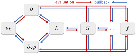
Figure 6: The schematic of chain rules in automatic differentiation with the logarithmic derivative related functions as the objective function.

$N$	M1		M2
	Computing	Memory	Computing	Memory
	time	allocation	time	allocation
$2$	4.46 $\mu$s	2.99 KB	5.14 $\mu$s	2.24 KB
$2^{2}$	18.09 $\mu$s	17.01 KB	11.17 $\mu$s	5.46  KB
$2^{3}$	257.65 $\mu$s	217.63 KB	35.84 $\mu$s	18.79 KB
$2^{4}$	4.55 ms	3.34 MB	151.51 $\mu$s	90.18 KB
$2^{5}$	174.61 ms	53.01 MB	962.17 $\mu$s	501.85 KB
$2^{6}$	9.45 s	846.18 MB	11.05 ms	3.31  MB
$2^{7}$	6151.51 s	137.95 GB	45.70 ms	230.98 MB
$2^{8}$	-	-	347.50 ms	1.73 GB
$2^{9}$	-	-	3.29 s	13.36 GB
$2^{10}$	-	-	41.51 s	105.08 GB

$\omega T$	5	10	15	20	30	40
GRAPE	5.23 s	21.75 s	44.95 s	71.00 s	178.56 s	373.89 s
auto-GRAPE	0.32 s	0.77 s	1.45 s	2.19 s	4.14 s	7.00 s

Table 2: Upper table: Comparison of the average computing time and memory allocation for the calculation of the gradient of QFI between two realization methods of AD. M1 and M2 represent the first and second methods. $N$ is the dimension of the density matrix. The density matrix and its derivative are generated randomly in the test. Lower table: Comparison of the average computing time per episode between GRAPE and auto-GRAPE with different target time $T$. Parallel computing is not applied here. KB, MB, and GB represent Kilobyte, Megabyte, and Gigabyte, respectively.

The core of AD is utilizing the chain rules to evaluate the derivatives of the objective function. As illustrated in Fig. 6, in AD the value of the objective function $f$ is evaluated from left to right (red arrows), and the derivatives are calculated backwards (blue arrows), which is also called pullback in the language of AD. In our case, the differentiation of $f$ on a control amplitude $u_{k}$ needs to be evaluated through all three paths, from $f$ to $\rho$, from $f$ to $\partial_{\mathbb{x}}\rho$ (if $f$ is a function of $\partial_{\mathbb{x}}\rho$) and from $f$ to $G$ to $L$. Here $L$ represents the SLDs of all parameters and $G:=G(L)=G(\rho,\partial_{\mathbb{x}}\rho)$ could be any intermediate function. For example, the contribution of the path from $f$ to $\rho$ to the derivative $\mathrm{d}f/\mathrm{d}u_{k}$ is $\frac{\partial f}{\partial\rho}\frac{\partial\rho}{\partial u_{k}}$. Notice that here $\partial f/\partial\rho$ is a formal derivative. The paths to $\rho$ and $\partial_{\mathbb{x}}\rho$ can be routinely solved in Zygote, however, the path to $L$ cannot be solved due to the entry-by-entry calculation of SLD in Eq. (9), which causes the difficulty to generate $\partial L/\partial\rho$ and $\partial L/\partial(\partial_{\mathbb{x}}\rho)$, and therefore $\partial G/\partial\rho$ and $\partial G/\partial(\partial_{\mathbb{x}}\rho)$ cannot be obtained. The chain rules in AD cannot be applied then. Hence, we need to manually provide $\partial G/\partial\rho$ and $\partial G/\partial(\partial_{\mathbb{x}}\rho)$ to let AD work in our case. To do it, one should first know that the total differentiation $\mathrm{d}G_{\alpha\beta}$ (the $\alpha\beta$th entry of $\mathrm{d}G$) can be evaluated via the equation

$$\mathrm{d}G_{\alpha\beta}=\sum_{ij}\frac{\partial G_{\alpha\beta}}{\partial L_{ij}}\mathrm{d}L_{ij}+\frac{\partial G_{\alpha\beta}}{\partial(L_{ij})^{*}}\mathrm{d}(L_{ij})^{*},$$ (47)

which can be written into a more compact matrix form

$$\mathrm{d}G_{\alpha\beta}=\mathrm{Tr}\!\left(\left(\frac{\partial G_{\alpha\beta}}{\partial L}\right)^{\mathrm{T}}\mathrm{d}L+\left(\frac{\partial G_{\alpha\beta}}{\partial L^{*}}\right)^{\mathrm{T}}\mathrm{d}L^{*}\right).$$ (48)

Due to the fact that the SLD is a Hermitian matrix, one can have $dL^{*}=dL^{\mathrm{T}}$, and the equation above reduces to

$$\mathrm{d}G_{\alpha\beta} =\mathrm{Tr}\!\left(\left(\frac{\partial G_{\alpha\beta}}{\partial L}\right)^{\mathrm{T}}\mathrm{d}L+\frac{\partial G_{\alpha\beta}}{\partial L^{\mathrm{T}}}\mathrm{d}L\right)$$

$$=2\mathrm{Tr}\!\left(\left(\frac{\partial G_{\alpha\beta}}{\partial L}\right)^{\mathrm{T}}\mathrm{d}L\right).$$ (49)

Now we introduce an auxiliary function $h$ which satisfies

$$\left(\frac{\partial G_{\alpha\beta}}{\partial L}\right)^{\mathrm{T}}=\rho h^{\mathrm{T}}+h^{\mathrm{T}}\rho.$$ (50)

This equation is a typical Lyapunov equation and can be numerically solved. Substituting the equation above into the expression of $\mathrm{d}G_{\alpha\beta}$, one can find that

$$\mathrm{d}G_{\alpha\beta}=2\mathrm{Tr}\left(h^{\mathrm{T}}\mathrm{d}L\rho+h^{\mathrm{T}}\rho\mathrm{d}L\right).$$ (51)

Due to the fact that $\partial_{\mathbb{x}}\rho=(\rho L+L\rho)/2$, we have $\rho\mathrm{d}L+(\mathrm{d}L)\rho=2\mathrm{d}(\partial_{\mathbb{x}}\rho)-(\mathrm{d}\rho)L-L\mathrm{d}\rho$, which means

$$\mathrm{d}G_{\alpha\beta}=2\mathrm{Tr}\!\left(2h^{\mathrm{T}}\mathrm{d}(\partial_{\mathbb{x}}\rho)\right)-2\mathrm{Tr}\!\left(\left(Lh^{\mathrm{T}}+h^{\mathrm{T}}L\right)\mathrm{d}\rho\right).$$ (52)

Next, since $G=G(\rho,\partial_{\mathbb{x}}\rho)$, $\mathrm{d}G_{\alpha\beta}$ can also be expressed by

$$\mathrm{d}G_{\alpha\beta}=2\mathrm{Tr}\!\left(\!\left(\frac{\partial G_{\alpha\beta}}{\partial\rho}\right)^{\!\mathrm{T}}\!\mathrm{d}\rho\!+\!\left(\frac{\partial G_{\alpha\beta}}{\partial(\partial_{\mathbb{x}}\rho)}\right)^{\!\mathrm{T}}\!\mathrm{d}(\partial_{\mathbb{x}}\rho)\!\right).$$ (53)

This equation is derived through a similar calculation procedure for Eq. (49). Comparing this equation with Eq. (52), one can see that

$$\frac{\partial G_{\alpha\beta}}{\partial\rho} =2h,$$ (54)

$$\frac{\partial G_{\alpha\beta}}{\partial(\partial_{\mathbb{x}}\rho)} =-hL^{\mathrm{T}}-L^{\mathrm{T}}h.$$ (55)

With these expressions, $\partial G/\partial\rho$ and $\partial G/\partial(\partial_{\mathbb{x}}\rho)$ can be obtained correspondingly. In this way, the entire path from $f$ to $L$ is connected. Together with the other two paths, AD can be fully applied in our case. The performance of computing time and memory allocation for the calculation of the gradient of QFI between these two realization methods of AD are compared with different dimensional density matrices. The dimension is denoted by $N$. As shown in the upper table in Table 2, the computing time and memory allocation of the second method are better than the first one except for the case of $N=2$, and this advantage becomes very significant when $N$ is large. Moreover, the computing time and memory allocation of the first method grow fast with the increase of dimension, which is reasonable as the calculations, especially the diagonalization, in the first method are performed in the $N^{2}$-dimensional space. There is no data of the first method when $N$ is larger than 7 as the memory occupation has exceeded our computer’s memory. From this comparison, one can see that the second method performs better than the first one in basically all aspects and hence is chosen as the default auto-GRAPE method in QuanEstimation.

Example. Consider the dynamics in Eq. (12) and control Hamiltonian in Eq. (45). Now define

$$\delta_{\mathrm{c}}\omega := 1/\sqrt{\mathcal{I}_{\omega\omega}},$$ (56)

$$\delta_{\mathrm{q}}\omega := 1/\sqrt{\mathcal{F}_{\omega\omega}}$$ (57)

as the theoretical optimal deviations with and without fixed measurement. The corresponding performance of controls generated via GRAPE and auto-GRAPE are shown in Figs. 7(a) and 7(b), which are obtained by 300 episodes in general. In QuanEstimation, the number of episodes can be set via the variable max_episode=300 in **kwargs in Table 1. As shown in these plots, the values of $\sqrt{\omega_{\mathrm{tr}}T}\delta_{\mathrm{q}}\omega$ in (a) and $\sqrt{\omega_{\mathrm{tr}}T}\delta_{\mathrm{c}}\omega$ in (b) obtained via GRAPE (red pentagrams) and auto-GRAPE (blue circles) basically coincide with each other, which is reasonable as they are intrinsically the same algorithm, just with different gradient calculation methods. However, auto-GRAPE shows a significant improvement on the computing time consumption, as given in the lower table in Table 2, especially for a large target time $T$. The growth of average computing time per episode with the increase of $T$ in auto-GRAPE is quite insignificant compared to that in GRAPE. Adam can be applied by setting Adam=True in **kwargs. For the sake of a good performance, one can set appropriate Adam parameters in **kwargs, including the learning rate epsilon, the exponential decay rate for the first (second) moment estimates beta1 (beta2). The default values of these parameters in the package are 0.01 and 0.90 (0.99). If Adam=False, the controls are updated with the constant step epsilon. Due to the convergence problem of Adam in some cases, several points in the figure are obtained by a second running of the code with a constant step, which takes the optimal control obtained in the first round (with Adam) as the initial guess.

In some scenarios, the time resolution of the control amplitude could be limited if the dynamics is too fast or the target time is too short. Hence, in the numerical optimization in such cases, the time steps of control cannot equal to that of the dynamics. Here we use the total control amplitude number $N_{\mathrm{c}}=T/\Delta t_{\mathrm{c}}$ with $\Delta t_{\mathrm{c}}$ the control time step, to represent the time resolution of the control and we assume $\Delta t_{\mathrm{c}}$ is fixed in the dynamics. A full $N_{\mathrm{c}}$ in Figs. 7(a) and 7(b) means $\Delta t_{\mathrm{c}}$ equals to the dynamical time step $\Delta t$. In the numerical calculation, it is possible that quotient of $\Delta t_{\mathrm{c}}$ by $\Delta t$ is not an integer, indicating that the existing time of all control amplitudes cannot be equivalent. To avoid this problem, in QuanEstimation the input number ($N_{t}$) of dynamical time steps is automatically adjusted to $kN_{\mathrm{c}}$ with $k$ the smallest integer to let $kN_{\mathrm{c}}>N_{t}$, if it is not already an integer multiple of $N_{\mathrm{c}}$. For example, if $N_{\mathrm{c}}=3$ and $N_{\mathrm{t}}=100$, then $N_{\mathrm{t}}$ is adjusted to 102. Notice that in the package GRAPE is not available to deal with a non-full $N_{\mathrm{c}}$ scenario for a technical reason. If GRAPE is invoked in this case, it would automatically go back to auto-GRAPE. As a matter of fact, auto-GRAPE outperforms GRAPE in most aspects, therefore, we strongly suggest the users choose auto-GRAPE, instead of GRAPE, in practice.

The performance of controls with limited $N_{\mathrm{c}}$ is also demonstrated in Figs. 7(a) and 7(b) with the dynamics in Eq. (12) and control Hamiltonian in Eq. (45). It can be seen that the constant-value controls ($N_{\mathrm{c}}=1$, orange upward triangles) cannot reduce the values of $\delta_{\mathrm{c}}\omega$ and $\delta_{\mathrm{q}}\omega$. In the case of fixed measurement it can only suppress the oscillation of $\delta_{\mathrm{c}}\omega$. The performance improves with the increase of $N_{\mathrm{c}}$ and when $N_{\mathrm{c}}=10$, the values of $\delta_{\mathrm{q}}\omega$ and $\delta_{\mathrm{c}}\omega$ are very close to those with a full $N_{\mathrm{c}}$. This fact indicates that inputting 10 control amplitudes is good enough in this case and a full $N_{\mathrm{c}}$ control is unnecessary. A limited $N_{\mathrm{c}}$ here could be easier to realize in practice and hence benefit the experimental realization.

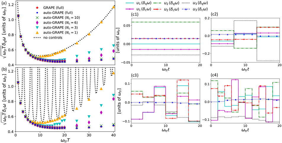
Figure 7: The performance of control-enhanced (a) $\sqrt{\omega_{\mathrm{tr}}T}\delta_{\mathrm{q}}\omega$ and (b) $\sqrt{\omega_{\mathrm{tr}}T}\delta_{\mathrm{c}}\omega$ with different $N_{\mathrm{c}}$. The optimal controls are generated via GRAPE and auto-GRAPE with the dynamics in Eq. (12) and control Hamiltonian in Eq. (45). The dotted black lines in (a) and (b) represent $\sqrt{\omega_{\mathrm{tr}}T}\delta_{\mathrm{q}}\omega$ and $\sqrt{\omega_{\mathrm{tr}}T}\delta_{\mathrm{c}}\omega$ without control. The red pentagrams are those obtained via GRAPE with a full $N_{\mathrm{c}}$, i.e., $N_{\mathrm{c}}$ equals to the number of time steps. The blue circles, green crosses, purple diamonds, cyan downward triangles and orange upward triangles represent those obtained via auto-GRAPE with $N_{\mathrm{c}}$ being full, 10, 6, 3 and 1, respectively. Other parameters are set to be the same with those in Fig. 2. (c1-c4) The optimal controls in the case of $\omega_{\mathrm{tr}}T=20$ with $N_{\mathrm{c}}$ being (c1) 1, (c2) 3, (c3) 6 and (c4) 10, respectively. The true value $\omega_{\mathrm{tr}}$ is set to be $1$. Planck units are applied here.

VI.3 Particle swarm optimization

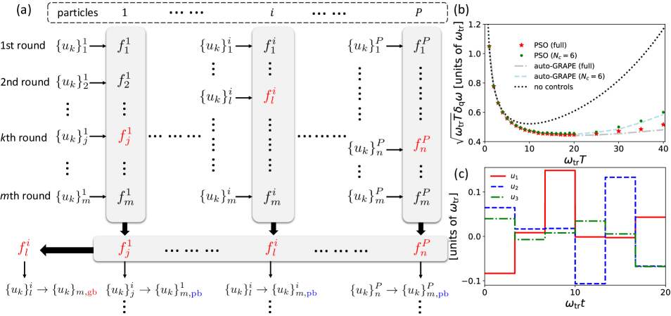
Figure 8: (a) Illustration of the basic operation of PSO in $m$th round of episode. The personal best (with the blue subscript pb) for each particle in this round is obtained by comparing all the values of $f$ of this particle in all previous rounds including the current one. The global best (with the red subscript gb) is obtained by comparing the values of $f$ of all personal bests in this round. The light gray areas represent the process of comparison, which takes the values of $\{u_{k}\}$ with respect to the maximum value of $f$. (b) The control-enhanced values of $\sqrt{\omega_{\mathrm{tr}}T}\delta_{\mathrm{q}}\omega$ with a full $N_{\mathrm{c}}$ (red pentagrams) and $N_{\mathrm{c}}=6$ (green circles), where the controls are generated via PSO. (c) The optimal controls for $N_{\mathrm{c}}=6$ in the case of $\omega_{\mathrm{tr}}T=20$. The true value $\omega_{\mathrm{tr}}$ is set to be $1$. Planck units are applied here.

Initialize the control $\left\{u_{k}\right\}^{i}_{1}$ for each $i\in\left[1,P\right]$;

Initialize $\left\{\delta u_{k}\right\}^{i}_{1}=0$ for each $i\in\left[1,P\right]$;

Assign $f(\left\{u_{k}\right\}^{i}_{0,\mathrm{pb}})=0$ for each $i\in\left[1,P\right]$;

for $m=1,M$  do

       for $i=1,P$  do

             Receive the control $\left\{u_{k}\right\}^{i}_{m}$;

             Evolve the state with $\left\{u_{k}\right\}^{i}_{m}$ and calculate the objective function $f(\left\{u_{k}\right\}^{i}_{m})$ at the target time $T$;

             Compare $f(\left\{u_{k}\right\}^{i}_{m})$ with value of the personal best in last episode $f(\left\{u_{k}\right\}^{i}_{m-1,\mathrm{pb}})$ and assign the new personal best $\left\{u_{k}\right\}^{i}_{m,\mathrm{pb}}=\mathrm{arg}\left(\max\left\{f(\left\{u_{k}\right\}^{i}_{m-1,\mathrm{pb}}),f(\left\{u_{k}\right\}^{i}_{m})\right\}\right)$;

       end for

      Compare all $f(\left\{u_{k}\right\}^{i}_{m,\mathrm{pb}})$ with $i\in[1,P]$ and assign the global best $\left\{u_{k}\right\}_{m,\mathrm{gb}}=\mathrm{arg}\left(\max\limits_{i\in\left[1,P\right]}f(\left\{u_{k}\right\}^{i}_{m,\mathrm{pb}})\right)$;

       for $i=1,P$  do

            Calculate $\left\{\delta u_{k}\right\}^{i}_{m}=c_{0}\left\{\delta u_{k}\right\}^{i}_{m-1}+\mathrm{rand}()\cdot c_{1}\big{(}\left\{u_{k}\right\}^{i}_{m,\mathrm{pb}}-\left\{u_{k}\right\}^{i}_{m}\big{)}+\mathrm{rand}()\cdot c_{2}\big{(}\left\{u_{k}\right\}_{m,\mathrm{gb}}-\left\{u_{k}\right\}^{i}_{m}\big{)}$;

             Update the control $\left\{u_{k}\right\}^{i}_{m+1}=\left\{u_{k}\right\}^{i}_{m}+\left\{\delta u_{k}\right\}^{i}_{m}$.

       end for

      

end for

Save the global best $\{u_{k}\}_{M,\mathrm{gb}}$ and corresponding $f$.

Algorithm 3 PSO

Particle swarm optimization (PSO) is a well-used gradient-free method in optimizations [67, 68], and has been applied in the detection of gravitational waves [69], the characterization of open systems [70], the prediction of crystal structure [71], and in quantum metrology it has been used to generate adaptive measurement schemes in phase estimations [72, 73].

A typical version of PSO includes a certain number (denoted by $P$) of parallel particles. In quantum control, these particles are just $P$ sets of controls $\{u_{k}\}$ labelled by $\{u_{k}\}^{i}$ for $i=1,\dots,P$. The value of $\{u_{k}\}$ of $i$th particle in $m$th round of episode is further denoted by $\{u_{k}\}^{i}_{m}$. The basic optimization philosophy of PSO is given in Fig. 8(a) and the pseudocode is given in Algorithm 3. In the pseudocode, $\left\{u_{k}\right\}^{i}_{0,\mathrm{pb}}$ and $f(\left\{u_{k}\right\}^{i}_{0,\mathrm{pb}})$ are just formal notations representing the initialization of the personal bests. There exist two basic concepts in PSO, the personal best and global best. In the $m$th round of episode, the personal best of $i$th particle ($\{u_{k}\}^{i}_{m,\mathrm{pb}}$) is assigned by the $\{u_{k}\}$ with respect to the maximum value of $f$ among all previous episodes of this particle, namely,

$$\{u_{k}\}^{i}_{m,\mathrm{pb}}=\mathrm{arg}\left(\max\limits_{n\in\left[1,m\right]}f(\left\{u_{k}\right\}^{i}_{n})\right)$$ (58)

with $\mathrm{arg}(\cdot)$ the argument. For example, as illustrated in Fig. 8, if $f^{1}_{j}$ is the maximum in $\{f^{1}_{1},f^{1}_{2},\dots,f^{1}_{m}\}$, then $\{u_{k}\}^{1}_{m,\mathrm{pb}}$ is assigned by $\{u_{k}\}^{1}_{j}$. Once the personal bests are obtained for all particles, the global best is assigned by the $\{u_{k}\}$ with respect to the maximum value of $f$ among all personal bests, i.e.,

$$\{u_{k}\}_{m,\mathrm{gb}}=\mathrm{arg}\left(\max\limits_{i\in\left[1,P\right]}f(\{u_{k}\}^{i}_{m,\mathrm{pb}})\right).$$ (59)

With all personal bests and the global best, the velocity $\{\delta u_{k}\}^{i}_{m}$ for the $i$th particle is calculated by

$$\{\delta u_{k}\}^{i}_{m}= c_{0}\{\delta u_{k}\}^{i}_{m-1}\!+\!\mathrm{rand}()\cdot c_{1}\left(\{u_{k}\}^{i}_{m,\mathrm{pb}}-\{u_{k}\}^{i}_{m}\right)$$

$$+\mathrm{rand}()\cdot c_{2}\left(\{u_{k}\}_{m,\mathrm{gb}}-\{u_{k}\}^{i}_{m}\right),$$ (60)

where rand() represents a random number within $[0,1]$ and $c_{0}$, $c_{1}$, $c_{2}$ are three positive constant numbers. In the package, these parameters can be adjusted in **kwargs, shown in Table 1, via the variables c0, c1 and c2. A typical choice for these constants is $c_{0}=1$, $c_{1}=c_{2}=2$, which are also the default values in the package. max_episode in **kwargs represents the episode number to run. If it is only set to be a number, for example max_episode=1000, the program will continuously run 1000 episodes. However, if it is a list, for example max_episode=[1000,100], the program will also run 1000 episodes in total but replace $\{u_{k}\}$ of all particles with the current global best every 100 episodes. p_num represents the particle number and is set to be 10 in default. The initial guesses of control can be input via ctrl0 and the default choice ctrl0=[] means all the guesses are randomly generated. In the case that the number of input guessed controls is less than the particle number, the algorithm will generate the remaining ones randomly. On the other hand, if the number is larger than the particle number, only the suitable number of controls will be used. The optimization result can be realized repeatedly by fixing the value of the variable seed, and its default value is 1234 in the package.

Initialize the control $\{u_{k}\}^{i}$ for $i\in[1,P]$;

Evolve the state with $\{u_{k}\}^{i}$ and calculate the objective function $f(\{u_{k}\}^{i})$ at the target time $T$ for $i\in[1,P]$;

for episode=1, $M$ do

       for $i=1,P$ do

             Randomly generate three integers $p_{1}$, $p_{2}$, $p_{3}$ in the regime $[1,P]$;

             Generate $\{G_{k}\}$ via the equation $\{G_{k}\}=\{u_{k}\}^{p_{1}}+c(\{u_{k}\}^{p_{2}}-\{u_{k}\}^{p_{3}})$;

             for $k=1,K$ do

                   Generate a random integer $a\in[1,N_{\mathrm{c}}]$;

                   for $j=1,N_{\mathrm{c}}$ do

                         Generate a random number $r\in[0,1]$ and assign $[Q_{k}]_{j}=\begin{cases}[G_{k}]_{j},&{\mathrm{if}\leavevmode\nobreak\ r\leq c_{r}\leavevmode\nobreak\ \mathrm{or}\leavevmode\nobreak\ j=a},\\ [u_{k}]_{j},&{\mathrm{if}\leavevmode\nobreak\ r>c_{r}\leavevmode\nobreak\ \mathrm{and}\leavevmode\nobreak\ j\neq a};\end{cases}$

                   end for

                  

             end for

            Evolve the state with the control $\{Q_{k}\}$ and calculate $f(\{Q_{k}\})$ at time $T$;

             if $f(\{u_{k}\}^{i})<f(\{Q_{k}\})$ then

                   Replace $\{u_{k}\}^{i}$ with $\{Q_{k}\}$.

             end if

            

       end for

      

end for

Compare all $f(\{u_{k}\}^{i})$ and save $\{u_{k}\}^{i}$ (and corresponding $f$) with respect to the largest $f$.

Algorithm 4 DE

Example. Here we also illustrate the performance of controls generated via PSO with the dynamics in Eq. (12) and control Hamiltonian in Eq. (45). $\delta_{\mathrm{q}}\omega$ is defined in Eq. (57). The performance of controls with a full $N_{\mathrm{c}}$ (red pentagrams) and $N_{\mathrm{c}}=6$ (green circles) are shown in Fig. 8(b), and the corresponding optimal controls for $N_{\mathrm{c}}=6$ are given in Fig. 8(c). Compared to the result obtained via auto-GRAPE (dash-dotted gray line for a full $N_{\mathrm{c}}$ and dashed light-blue line for $N_{\mathrm{c}}=6$), the performance of PSO is worse than that of auto-GRAPE, especially in the case of a large target time $T$ with a full $N_{\mathrm{c}}$. This is due to the fact that the search space is too large for PSO in such cases as the time step $\Delta t$ is fixed in the calculation and a larger $T$ means a larger value of $N_{\mathrm{c}}$. For example, in the case of $\omega_{\mathrm{tr}}T=40$ and $N_{\mathrm{c}}=10000$, the total parameter number in the optimization is 30000. PSO can provide a good performance when the dimension of the search space is limited. In the case of $N_{\mathrm{c}}=6$, the result of PSO basically coincides with that of auto-GRAPE. Hence, for those large systems that the calculation of gradient is too time-consuming or the search space is limited, the gradient-free methods like PSO would show their powers.

VI.4 Differential evolution

Figure 9: (a) Illustration of the optimization process of DE, which includes four steps: initialization, mutation, crossover and selection. (b) The control-enhanced values of $\sqrt{\omega_{\mathrm{tr}}T}\delta_{\mathrm{q}}\omega$ with a full $N_{\mathrm{c}}$ (red pentagrams) and $N_{\mathrm{c}}=6$ (green circles), where the controls are generated via DE. (c) The optimal controls for $N_{\mathrm{c}}=6$ in the case of $\omega_{\mathrm{tr}}T=20$. The true value $\omega_{\mathrm{tr}}$ is set to be $1$. Planck units are applied here.

Differential evolution (DE) is another useful gradient-free algorithm in optimizations [74]. It has been used to design adaptive measurements in quantum phase estimation [75, 76], high-quality control pulses in quantum information [77, 78], and help to improve the learning performance in quantum open systems [79, 80]. Different with PSO, DE would not converge prematurely in general and its diversification is also better since the best solution does not affect other solutions in the population [81].

A typical DE includes a certain number (denoted by $P$) of $\{u_{k}\}^{i}$, which is usually referred to as the populations in the language of DE. In QuanEstimation, the population number and the guessed controls can be set via the variables p_num and ctrl0 in **kwargs, as shown in Table 1. The rule for the usage of ctrl0 here is the same as ctrl0 in PSO. After the initialization of all $\{u_{k}\}^{i}$ ($i\in[1,P]$), two important processes in DE, mutation and crossover, are performed, as illustrated in Fig. 9(a) with the pseudocode in Algorithm 4. In the step of mutation, three populations $\{u_{k}\}^{p_{1}}$, $\{u_{k}\}^{p_{2}}$ and $\{u_{k}\}^{p_{3}}$ are randomly picked from all $\{u_{k}\}^{i}$, and used to generate a new population $\{G_{k}\}$ via the equation

$$\{G_{k}\}=\{u_{k}\}^{p_{1}}+c(\{u_{k}\}^{p_{2}}-\{u_{k}\}^{p_{3}})$$ (61)

with $c\in[0,1]$ (or $[0,2]$) a constant number. The next step is the crossover. At the beginning of this step, a random integer $a$ is generated in the regime $[1,N_{\mathrm{c}}]$, which is used to make sure the crossover happens definitely. Then another new population $\{Q_{k}\}$ is generated for each $\{u_{k}\}^{i}$ utilizing $\{G_{k}\}$. Now we take $j$th entry of $Q_{k}$ ($[Q_{k}]_{j}$) as an example to show the generation rule. In the first, a random number $r$ is picked in the regime $[0,1]$. Then $[Q_{k}]_{j}$ is assigned via the equation

$$[Q_{k}]_{j}=\begin{cases}[G_{k}]_{j},&{\mathrm{if}\leavevmode\nobreak\ r\leq c_{r}\leavevmode\nobreak\ \mathrm{or}\leavevmode\nobreak\ j=a},\\ [u_{k}]_{j},&{\mathrm{if}\leavevmode\nobreak\ r>c_{r}\leavevmode\nobreak\ \mathrm{and}\leavevmode\nobreak\ j\neq a},\end{cases}$$ (62)

where $[G_{k}]_{j}$ is the $j$th entry of $G_{k}$ and $[u_{k}]_{j}$ is the $j$th entry of a $u_{k}$ in $\{u_{k}\}^{i}$. This equation means if $r$ is no larger than a given constant $c_{r}$ (usually called crossover constant in DE), then assign $[G_{k}]_{j}$ to $[Q_{k}]_{j}$, otherwise assign $[u_{k}]_{j}$ to $[Q_{k}]_{j}$. In the meantime, the $a$th entry of $Q_{k}$ always takes the value of $[G_{k}]_{j}$ regardless the value of $r$ to make sure at least one point mutates. After the crossover, the values of objective functions $f(\{u_{k}\}^{i})$ and $f(\{Q_{k}\})$ are compared, and $\{u_{k}\}^{i}$ is replaced by $\{Q_{k}\}$ if $f(\{Q_{k}\})$ is larger. In the package, $c$ and $c_{r}$ can be adjusted via the variables c and cr in **kwargs, and the default values are 1.0 and 0.5.

Example. The performance of controls generated via DE is also illustrated with the dynamics in Eq. (12) and control Hamiltonian in Eq. (45). $\delta_{\mathrm{q}}\omega$ is defined in Eq. (57). As shown in Fig. 9(b), different with PSO, the performance of DE with a full $N_{\mathrm{c}}$ (red pentagrams) is very close to that of auto-GRAPE (dash-dotted gray line), even for a large target time $T$, which indicates that DE works better than PSO in this example. More surprisingly, in the case of $N_{\mathrm{c}}=6$, DE (green circles) not only outperforms PSO, but also significantly outperforms auto-GRAPE (dashed light-blue line). This result indicates that no algorithm has the absolute advantage in general. Comparison and combination of different algorithms are a better approach to design optimal controls in quantum metrology, which can be conveniently finished via QuanEstimation. The optimal controls obtained via DE for $N_{\mathrm{c}}=6$ are given in Fig. 9(c) in the case of $\omega_{\mathrm{tr}}T=20$. The results above are obtained with 1000 episodes, which can be adjusted via max_episode=1000 in **kwargs.

VI.5 Deep Deterministic Policy Gradients

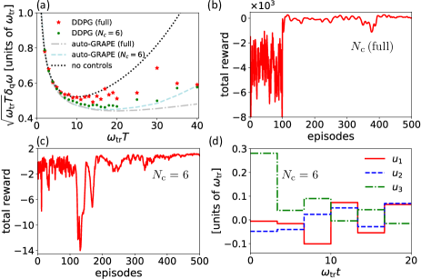
Figure 10: (a) The control-enhanced values of $\sqrt{\omega_{\mathrm{tr}}T}\delta_{\mathrm{q}}\omega$ with a full $N_{\mathrm{c}}$ (red pentagrams) and $N_{\mathrm{c}}=6$ (green circles), where the controls are generated via DDPG. (b-c) The change of total reward in the episodes in the case of (b) a full $N_{\mathrm{c}}$ and (c) $N_{\mathrm{c}}=6$. (d) The controls obtained via DDPG for $N_{\mathrm{c}}=6$ in the case of $\omega_{\mathrm{tr}}T=20$. The true value $\omega_{\mathrm{tr}}$ is set to be $1$. Planck units are applied here.

Deep deterministic policy gradients (DDPG) is a powerful tool in machine learning [82] and has already been applied in quantum physics to perform quantum multiparameter estimation [61] and enhance the generation of spin squeezing [83]. The pseudocode of DDPG for quantum estimation and the corresponding flow chart can be found in Ref. [17], and the details will not be repeatedly addressed herein.

Example. The performance of controls generated via DDPG in the case of single-parameter estimation is also illustrated with the dynamics in Eq. (12) and control Hamiltonian in Eq. (45), as shown in Fig. 10(a). $\delta_{\mathrm{q}}\omega$ is defined in Eq. (57). The reward is taken as the logarithm of the ratio between the controlled and non-controlled values of the QFI at time $t$. It can be seen that the performance of DDPG with a full $N_{\mathrm{c}}$ (red pentagrams) shows a significant disparity with that of auto-GRAPE (dash-dotted gray line). A more surprising fact is that it is even worse than the performance of both auto-GRAPE (dashed light-blue line) and DDPG (green circles) with $N_{\mathrm{c}}=6$. And the performance of DDPG with $N_{\mathrm{c}}=6$ also presents no advantage compared to PSO and DE. However, we cannot rashly say that PSO and DE outperform DDPG here as DDPG involves way more parameters and maybe a suitable set of parameters would let its performance comparable or even better than PSO and DE. Nevertheless, we can still safely to say that PSO and DE, especially DE, are easier to find optimal controls in this example and DDPG does not present a general advantage here. The total reward in the case of $\omega_{\mathrm{tr}}T=20$ with a full $N_{\mathrm{c}}$ and $N_{\mathrm{c}}=6$ are given in Figs. 10(b) and 10(c), respectively. The total reward indeed increases and converges for a full $N_{\mathrm{c}}$, but the final performance is only sightly better than the non-controlled value [dotted black line in Fig. 10(a)]. For $N_{\mathrm{c}}=6$, the total reward does not significantly increase, which means the corresponding performance of $\delta_{\mathrm{q}}\omega$ basically comes from the average performance of random controls. The controls obtained via DDPG for $N_{\mathrm{c}}=6$ are shown in Fig. 10(d).

VI.6 Performance of the convergence speed

Apart from the improvement of the objective function, the convergence speed is also an important aspect of an algorithm to evaluate its performance. Here we illustrate the convergence performance of different algorithms in Fig. 11 in the single-parameter scenario discussed previously, namely, the dynamics in Eq. (12) and control Hamiltonian in Eq. (45) with a full $N_{\mathrm{c}}$. As shown in Fig. 11(a), GRAPE (dashed red line) and auto-GRAPE (dotted black line) show higher convergence speed than PSO (solid green line) and DE (dash-dotted cyan line). This phenomenon coincides with the common understanding that the gradient-based methods converge faster than gradient-free methods in general. DE converges slower than GRAPE and auto-GRAPE, but the final performance of QFI basically coincides with them. PSO presents the slowest speed in this example and the final result of QFI is also worse than others. DDPG is not involved in this figure as its improvement on the QFI is not as significant as others.

The effect of Adam in auto-GRAPE is also illustrated in Fig. 11(b). Denote $\epsilon$ as the learning rate in Adam. In the case of constant-step update, auto-GRAPE with $\epsilon=0.01$ (dotted black line) converges faster than that with $\epsilon=0.005$ (dash-dotted green line), which is common and reasonable as a large step usually implies a higher convergence speed. However, when Adam is invoked, this difference becomes very insignificant and both lines (solid gray line for $\epsilon=0.01$ and dashed blue line for $\epsilon=0.005$) converge faster than constant-step updates. However, it should be noticed that a large $\epsilon$ in Adam may result in a strong oscillation of $\delta_{\mathrm{q}}\omega$ in the episodes, and it should be adjusted to smaller values if one wants to avoid this phenomenon.

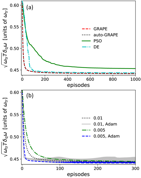
Figure 11: (a) The convergence performance of different algorithms, including GRAPE (dashed red line), auto-GRAPE (dotted black line), PSO (solid green line) and DE (dash-dotted cyan line). (b) The convergence performance of auto-GRAPE with constant step $\epsilon=0.01$ (dotted black line), $\epsilon=0.005$ (dash-dotted green line), and with Adam (solid gray line for $\epsilon=0.01$ and dashed blue line for $\epsilon=0.005$). The target time $\omega_{\mathrm{tr}}T=20$, and the true value $\omega_{\mathrm{tr}}$ is set to be 1. Planck units are applied here.

VI.7 Multiparameter estimation

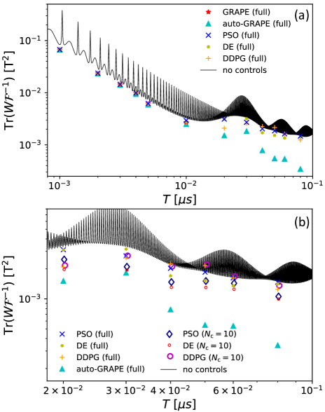
Figure 12: (a) The performance of controls generated via different algorithms, including GRAPE (red pentagrams), auto-GRAPE (cyan triangles) with full $N_{\mathrm{c}}$, PSO (blue crosses) with full $N_{\mathrm{c}}$, DE (yellow circles) with full $N_{\mathrm{c}}$ and DDPG (orange pluses) with full $N_{\mathrm{c}}$. (b) The performance of controls generated via PSO (dark blue diamonds), DE (small red hollow circles) and DDPG (large purple hollow circles) with limited $N_{\mathrm{c}}$ ($N_{\mathrm{c}}=10$). $W$ is chosen to be $\openone$.

Compared to the single-parameter estimation, multiparameter estimation is a more challenging problem in quantum metrology. In this case, $\mathrm{Tr}(W\mathcal{F}^{-1})$ cannot be used as the objective function in the implementation of GRAPE as the analytical calculation of $\mathcal{F}^{-1}$ is very difficult, if not fully impossible, when the number of parameter is large. Hence, in GRAPE when $W=\openone$, $\sum_{a}1/\mathcal{F}_{aa}$, a lower bound of $\mathrm{Tr}(\mathcal{F}^{-1})$, is taken as the superseded objective function [13, 56, 17]. Unfortunately, $\sum_{a}W_{aa}/\mathcal{F}_{aa}$ fails to be a valid lower bound for a general $W$. In this case, to keep $\sum_{a}W_{aa}/\mathcal{F}_{aa}$ a valid lower bound, the parameters for estimation have to be reorganized by the linear combination of the original ones to let $W$ be diagonal, which causes the inconvenience to implement GRAPE insuch cases. Different with GRAPE, this problem naturally vanishes in auto-GRAPE as the inverse matrix $\mathcal{F}^{-1}$ is calculated automatically and so does the gradient. In the meantime, PSO and DE would also not face such problems as they are gradient-free.

Example. Here we take an electron-nuclear spin system, which can be readily realized in the nitrogen-vacancy centers, as an example to demonstrate and compare the performance of different algorithms included in QuanEstimation. The Hamiltonian of this system reads [86, 84, 85]

$$H_{0}/\hbar=DS^{2}_{3}+g_{\mathrm{S}}\vec{B}\cdot\vec{S}+g_{\mathrm{I}}\vec{B}\cdot\vec{I}+\vec{S}^{\,\mathrm{T}}\mathcal{A}\vec{I},$$ (63)

where $S_{i}=s_{i}\otimes\openone$ and $I_{i}=\openone\otimes\sigma_{i}$ ($i=1,2,3$) represent the electron and nuclear (${}^{15}\mathrm{N}$) operators with $s_{1}$, $s_{2}$ and $s_{3}$ spin-1 operators. Their specific expressions are

$$s_{1}=\frac{1}{\sqrt{2}}\left(\begin{array}[]{ccc}0&1&0\\ 1&0&1\\ 0&1&0\end{array}\right),s_{2}=\frac{1}{\sqrt{2}}\left(\begin{array}[]{ccc}0&-i&0\\ i&0&-i\\ 0&i&0\end{array}\right)\!\!,$$ (70)

and $s_{3}=\mathrm{diag}(1,0,-1)$. The vectors $\vec{S}=(S_{1},S_{2},S_{3})^{\mathrm{T}}$, $\vec{I}=(I_{1},I_{2},I_{3})^{\mathrm{T}}$ and $\mathcal{A}$ is the hyperfine tensor. In this case, $\mathcal{A}=\mathrm{diag}(A_{1},A_{1},A_{2})$ with $A_{1}$ and $A_{2}$ the axial and transverse magnetic hyperfine coupling coefficients. The hyperfine coupling between the magnetic field and electron are approximated to be isotopic. The coefficients $g_{\mathrm{S}}=g_{\mathrm{e}}\mu_{\mathrm{B}}/\hbar$ and $g_{\mathrm{I}}=g_{\mathrm{n}}\mu_{\mathrm{n}}/\hbar$. Here $g_{\mathrm{e}}$ ($g_{\mathrm{n}}$) is the $g$ factor of the electron (nuclear), $\mu_{\mathrm{B}}$ ($\mu_{\mathrm{n}}$) is the Bohr (nuclear) magneton and $\hbar$ is the Plank’s constant. The control Hamiltonian is

$$H_{\mathrm{c}}/\hbar=\sum^{3}_{i=1}\Omega_{i}(t)S_{i},$$ (71)

where $\Omega_{i}(t)$ is a time-varying Rabi frequency. In practice, the electron suffers from the noise of dephasing, which means the dynamics of the full system is described by the master equation

$$\partial_{t}\rho=-i[H_{0}+H_{\mathrm{c}},\rho]+\frac{\gamma}{2}(S_{3}\rho S_{3}-S^{2}_{3}\rho-\rho S^{2}_{3}),$$ (72)

with $\gamma$ the dephasing rate, which is usually inverse proportional to the dephasing time $T^{*}_{2}$.

Now we use this system as a controllable magnetometer to estimate the magnetic field $\vec{B}$, which is a three-parameter estimation problem. The optimal controls can be obtained via different algorithms. In this case, the initial state is taken as $(|1\rangle+|\!-\!1\rangle)\otimes|\!\!\uparrow\rangle/\sqrt{2}$, where $(|1\rangle+|\!-\!1\rangle)/\sqrt{2}$ is an electron state with $|1\rangle$ ($|\!-\!1\rangle$) the eigenstate of $s_{3}$ corresponding to the eigenvalue $1$ ($-1$). $|\!\!\uparrow\rangle$ is a nuclear state and the eigenstate of $\sigma_{3}$ corresponding to the eigenvalue 1. $W$ is chosen to be $\openone$. The systematic parameters are chosen as $D=2\pi\times 2.87$ GHz, $g_{\mathrm{S}}=2\pi\times 28.03$ GHz/T, $g_{\mathrm{I}}=2\pi\times 4.32$ MHz/T, $A_{1}=2\pi\times 3.65$ MHz, $A_{2}=2\pi\times 3.03$ MHz, and the true values of $\vec{B}$ are $B_{1}=B_{2}=B_{3}=0.50$ mT. The dephasing rate $\gamma=2\pi\times 1$ MHz. All the parameter values are selected according to Refs. [86, 87].

The performance of controls given by different algorithms is given in Fig. 12. The control amplitude is limited in the regime $[-20\,\mathrm{MHz},20\,\mathrm{MHz}]$. In the case of a full $N_{\mathrm{c}}$ [$N_{\mathrm{c}}=2000T/(0.01\,\mathrm{\mu s})$], as shown in Fig. 12(a), the performance of GRAPE (red pentagrams), auto-GRAPE (cyan triangles), PSO (blue crosses), DE (yellow circles) and DDPG (orange pluses) basically coincide for small target time ($T\leq 0.01\,\mathrm{\mu s}$), and the reduction of $\mathrm{Tr}(W\mathcal{F}^{-1})$ is limited compared to the non-controlled values (solid black line). In the regime of large target time ($T>0.01\,\mathrm{\mu s}$), auto-GRAPE shows the best performance. GRAPE is not applied in these points as its time consumption is too heavy for our computers. PSO and DE only find controls that provide slightly enhancement on $\mathrm{Tr}(W\mathcal{F}^{-1})$ in this regime. The different behaviors of the performance are due to the large search space in this case. For example, the total control number for $T=0.08\,\mathrm{\mu s}$ is 48000 including all three controls $\Omega_{1}$, $\Omega_{2}$ and $\Omega_{3}$. In such a large parameter space, different with the gradient-based methods, the gradient-free methods cannot promise to find optimal values. Hence, the gradient-based methods would be a good choice in such cases. However, one should notice that the gradient-based methods like auto-GRAPE could be more memory consuming than gradient-based methods. In the case that the computer memory is limited, one may have to choose gradient-free methods.

In the case of a small search space, for example $N_{\mathrm{c}}=10$, the performance of PSO and DE improve significantly, as shown in Fig. 12(b). Both PSO (dark blue diamonds) and DE (small red hollow circles) with $N_{\mathrm{c}}=10$ outperform the full $N_{\mathrm{c}}$ cases, yet DDPG with $N_{\mathrm{c}}=10$ (large purple hollow circles) does not show this behavior. Similar to the single-parameter scenario, DE provides a better performance than PSO and DDPG when the control number $N_{\mathrm{c}}$ is limited. A more interesting fact is that for some target time, like $T=0.03\,\mathrm{\mu s}$, PSO and DE even provide comparable performance with auto-GRAPE with a full $N_{\mathrm{c}}$, indicating that the control schemes given by PSO and DE in this case not only meet the best precision limit, but are also simpler to implement in experiments than the full-$N_{\mathrm{c}}$ scheme given by auto-GRAPE.

VI.8 Minimum parameterization time optimization

The control optimizations discussed in the previous subsections are performed with a fixed target time $T$. In some scenarios, the goal is not to achieve the highest precision within a fixed time, but to reach a given precision as soon as possible. This problem requires the search of minimum time to reach a given value of the objective function, which can be realized in QuanEstimation in the class ControlOpt(). After the callings of control=ControlOpt() and control.dynamics(), one can use the following code to solve this problem:

⬇

control.mintime(f,W=[],M=[],method="binary",

target="QFIM",LDtype="SLD")

Here the input f is a float number representing the given value of the objective function. The type of objective function can be adjusted via target=" ", which includes three options "QFIM" (default), "CFIM", and "HCRB". The measurement can be input via M=[] if necessary, and in this case the objective function will be chosen as the CFIM regardless of the setting in target=" ". In the case of target="QFIM", the type of QFIM can be changed via LDtype=" ". The choices include "SLD", "RLD", and "LLD". method="binary" represents the binary search (logarithmic search) and method="forward" represents the forward search from the beginning of time. Choosing a suitable method may help to improve the calculation efficiency. For example, if the users already know that the minimum time is very small compared to $T$, the forward search would be more efficient than the binary search. Notice that the search is restricted in the regime $[0,T]$ where $T$ is given by the array tspan input in ControlOpt(), and the current code can only deal with full-$N_{\mathrm{c}}$ controls. The outputs are two files "mtspan.csv" and "controls.csv" containing the array of time from the start to the searched minimum time and the corresponding length of optimal controls, respectively.

VII State optimization

Algorithms	method=	**kwargs and default values
AD	"AD"	"Adam"	False
		"psi0"	[]
		"max_episode"	300
		"epsilon"	0.01
		"beta1"	0.90
		"beta2"	0.99
PSO	"PSO"	"p_num"	10
		"psi0"	[]
		"max_episode"	[1000,100]
		"c0"	1.0
		"c1"	2.0
		"c2"	2.0
		"seed"	1234
DE	"DE"	"p_num"	10
		"psi0"	[]
		"max_episode"	1000
		"c"	1.0
		"cr"	0.5
		"seed"	1234
NM	"NM"	"p_num"	10
		"psi0"	[]
		"max_episode"	1000
		"ar"	1.0
		"ae"	2.0
		"ac"	0.5
		"as0"	0.5
		"seed"	1234
RI	"RI"	"psi0"	[]
		"max_episode"	300
		"seed"	1234
DDPG	"DDPG"	"psi0"	[]
		"max_episode"	500
		"layer_num"	3
		"layer_dim"	200
		"seed"	1234

Table 3: Available methods for state optimization in QuanEstimation and corresponding default parameter settings. Notice that AD is not available when the HCRB are taken as the objective function.

Quantum resources like entanglement and squeezing are key in quantum parameter estimation to demonstrate a quantum enhanced precision. In contrast to the dynamical resources like time or control, entanglement and squeezing are usually embedded in the probe state, indicating that different probe states would present dramatically different performance on the precision. The search of optimal probe states is thus an essential step in the design of optimal schemes. Various methodologies, including direct analytical calculations [88, 89, 90, 91, 92, 93, 95, 94, 96, 97, 98, 99, 100, 101], semi-analytical [102, 103, 104, 105, 106, 107, 108, 109, 110] and full numerical approaches [112, 113, 111, 114, 115], have been proposed and discussed. More advances of the state optimization in quantum metrology can be found in a recent review [17]. QuanEstimation includes the process of state optimization with various methods, including both gradient-based and gradient-free methods. The specific code in QuanEstimation for the execution of state optimization are as follows:

⬇

state = StateOpt(savefile=False,method="AD",

**kwargs)

state.dynamics(tspan,H0,dH,Hc=[],ctrl=[],

decay=[],dyn_method="expm")

state.QFIM(W=[],LDtype="SLD")

state.CFIM(M=[],W=[])

In the case that the parameterization is described by the Kraus operators, replace state.dynamics() with the code state.Kraus(K,dK). The parameters above have already been introduced previously. The default settings W=[] and M=[] means $W=\openone$ and the measurement is a SIC-POVM. The optimization method can be adjusted via method=" " and corresponding parameters can be set via **kwargs. The available optimization methods and corresponding default parameter settings are given in Table 3. The dynamics can also be solved with ODE by setting dyn_method="ode". One exception is that when method="AD" is applied. In this case ODE is not available for now. Two files "f.csv" and "states.csv" will be generated at the end of the program, which include the values of the objective function in all episodes and the final obtained optimal probe state. When savefile=True, the states obtained in all episodes will be saved in "states.csv". In the multiparameter estimation, the HCRB can also be chosen as the objective function by calling the code:

⬇

state.HCRB(W=[])

Notice that if method="AD", state.HCRB() is not available. Similar to the control optimization, if the users invoke state.HCRB() in the single-parameter scenario, a warning will arise to remind them to call state.QFIM() instead.

Receive the guessed probe state $\rho_{0}=|\psi_{\mathrm{in}}\rangle\langle\psi_{\mathrm{in}}|$;

for episode=1, $M$ do

       Calculate the density matrix $\rho_{T}$ and its derivative $\partial_{\mathbb{x}}\rho_{T}$ at the target time $T$;

       Calculate the objective function $f(T)$ with $\rho_{T}$ and $\partial_{\mathbb{x}}\rho_{T}$;

       Calculate the gradients $\big{\{}\frac{\delta f(T)}{\delta c_{i}}\big{\}}$ with the automatic differentiation;

       Update the coefficients $\{c_{i}\}\leftarrow\{c_{i}\}+\epsilon\big{\{}\frac{\delta f(T)}{\delta c_{i}}\big{\}}$;

       Normalize the coefficients $\{c_{i}\}\leftarrow\frac{1}{\sqrt{\sum_{j}|c_{j}|^{2}}}\{c_{i}\}$.

end for

Save the coefficients and corresponding $f(T)$, and reconstruct the state.

Algorithm 5 AD for pure states

In the previous section, we already showed the power of automatic differentiation (AD) in the construction of auto-GRAPE. Similarly, it can also be used in the state optimization. Due to the convexity of the QFI and QFIM [11, 13], the optimal probe states are pure states in most scenarios. Hence, we first consider the state optimization within the set of pure states. The pseudocode of AD in state optimization for pure states is given in Algorithm 5. In a specific basis $\{|i\rangle\langle i|\}$, a probe state could be expanded by $|\psi\rangle=\sum_{i}c_{i}|i\rangle$, and the search of optimal probe states is equivalent to the search of a set of normalized complex coefficients $\{c_{i}\}$. In AD, a guessed probe state is first given or generated and evolved to the target time $T$ according to the given dynamics, during which the density matrices and corresponding derivatives with respect to $\mathbb{x}$ are calculated and saved. Then after calculating the objective function $f(T)$ at time $T$, all gradients $\{\delta f(T)/\delta c_{i}\}$ are evaluated via the automatic differentiation, and the coefficients $\{c_{i}\}$ are updated accordingly with the step $\epsilon$. This step can be adjusted via epsilon in **kwargs. Finally, the updated coefficients are normalized as required by the quantum mechanics. In the package, Adam is not applied by default in AD and it can be turned on by setting Adam=True in **kwargs.

Regarding the gradient-free methods, apart from the PSO, DE and DDPG, QuanEstimation also contains the Nelder-Mead algorithm (NM) [116], which has already been used by Fröwis et al. [112] to perform the state optimization in the case of collective spins. The detailed flow chart of NM to locate the minimum value of an objective function can be found in Ref. [17]. For the sake of self-consistency of the paper, here we present its pseudocode in Algorithm 6 for the search of the maximum value of $f$ at the target time $T$.

Receive a set of guessed states $|\psi_{1}\rangle,\cdots,|\psi_{n+1}\rangle$;

for episode=1, $M$ do

       Evolve all states according to the given dynamics and calculate the objective function $f$ at time $T$;

       Sort the states and reassign the indices to let $f(|\psi_{1}\rangle)\geq f(|\psi_{2}\rangle)\geq\cdots\geq f(|\psi_{n+1}\rangle)$;

       Calculate the average state $|\psi_{\mathrm{a}}\rangle=\frac{1}{\sqrt{\mathcal{N}_{\mathrm{a}}}}\sum^{n}_{k=1}|\psi_{k}\rangle$;

       Calculate the reflected state $|\psi_{\mathrm{r}}\rangle=\frac{1}{\sqrt{\mathcal{N}_{\mathrm{r}}}}[|\psi_{\mathrm{a}}\rangle+a_{\mathrm{r}}(|\psi_{\mathrm{a}}\rangle-|\psi_{n+1}\rangle)]$;

       if $f(|\psi_{\mathrm{r}}\rangle)>f(|\psi_{1}\rangle)$ then

            Calculate the expanded state $|\psi_{\mathrm{e}}\rangle=\frac{1}{\sqrt{\mathcal{N}_{\mathrm{e}}}}[|\psi_{\mathrm{a}}\rangle+a_{\mathrm{e}}(|\psi_{\mathrm{r}}\rangle-|\psi_{\mathrm{a}}\rangle)]$;

             if $f(|\psi_{\mathrm{r}}\rangle)\geq f(|\psi_{\mathrm{e}}\rangle)$ then

                  Replace $|\psi_{n+1}\rangle$ with $|\psi_{\mathrm{r}}\rangle$;

            else

                  Replace $|\psi_{n+1}\rangle$ with $|\psi_{\mathrm{e}}\rangle$;

             end if

            

       else if $f(|\psi_{1}\rangle)\geq f(|\psi_{\mathrm{r}}\rangle)>f(|\psi_{n}\rangle)$ then

            Replace $|\psi_{n+1}\rangle$ with $|\psi_{\mathrm{r}}\rangle$;

       else if $f(|\psi_{n}\rangle)\geq f(|\psi_{\mathrm{r}}\rangle)>f(|\psi_{n+1}\rangle)$ then

            Calculate the outside contracted state $|\psi_{\mathrm{oc}}\rangle=\frac{1}{\sqrt{\mathcal{N}_{\mathrm{oc}}}}[|\psi_{\mathrm{a}}\rangle+a_{\mathrm{c}}(|\psi\rangle_{\mathrm{r}}-|\psi_{\mathrm{a}}\rangle)]$;

             if $f(|\psi_{\mathrm{oc}}\rangle)\geq f(|\psi_{\mathrm{r}}\rangle)$ then

                  Replace $|\psi_{n+1}\rangle$ with $|\psi_{\mathrm{oc}}\rangle$;

            else

                  Replace all $|\psi_{k}\rangle$ for $k\in[2,n+1]$ with $\frac{1}{\sqrt{\mathcal{N}_{k}}}[|\psi_{1}\rangle+a_{\mathrm{s}}(|\psi_{k}\rangle-|\psi_{1}\rangle)]$;

             end if

            

       else

            Calculate the inside contracted state $|\psi_{\mathrm{ic}}\rangle=\frac{1}{\sqrt{\mathcal{N}_{\mathrm{ic}}}}[|\psi_{\mathrm{a}}\rangle-a_{\mathrm{c}}(|\psi_{\mathrm{a}}\rangle-|\psi_{n+1}\rangle)]$;

             if $f(|\psi_{\mathrm{ic}}\rangle)>f(|\psi_{n+1}\rangle)$ then

                  Replace $|\psi_{n+1}\rangle$ with $|\psi_{\mathrm{ic}}\rangle$;

            else

                  Replace all $|\psi_{k}\rangle$ for $k\in[2,n+1]$ with $\frac{1}{\sqrt{\mathcal{N}_{k}}}[|\psi_{1}\rangle+a_{\mathrm{s}}(|\psi_{k}\rangle-|\psi_{1}\rangle)]$;

             end if

            

       end if

      

end for

Return the optimal state $|\psi_{1}\rangle$ and corresponding $f$.

Algorithm 6 NM for pure states

In NM, $n+1$ guessed states are input and sorted descendingly according to the corresponding values of $f$, namely, $f(|\psi_{1}\rangle)\geq\cdots\geq f(|\psi_{n+1}\rangle)$. In one episode of optimization, the average state $|\psi_{\mathrm{a}}\rangle:=\frac{1}{\sqrt{\mathcal{N}_{\mathrm{a}}}}\sum^{n}_{k=1}|\psi_{k}\rangle$ and reflected state $|\psi_{\mathrm{r}}\rangle:=\frac{1}{\sqrt{\mathcal{N}_{\mathrm{r}}}}[|\psi_{\mathrm{a}}\rangle+a_{\mathrm{r}}(|\psi_{\mathrm{a}}\rangle-|\psi_{n+1}\rangle)]$ are first calculated. In the case that the reflected state is better than $|\psi_{1}\rangle$, i.e., $f(|\psi_{\mathrm{r}}\rangle)$ is larger than $f(|\psi_{1}\rangle)$, the expanded state $|\psi_{\mathrm{e}}\rangle:=\frac{1}{\sqrt{\mathcal{N}_{\mathrm{e}}}}[|\psi_{\mathrm{a}}\rangle+a_{\mathrm{e}}(|\psi_{\mathrm{r}}\rangle-|\psi_{\mathrm{a}}\rangle)]$ is then calculated and compared to the reflected state. If the reflected state is still better, then replace $|\psi_{n+1}\rangle$ with $|\psi_{\mathrm{r}}\rangle$, otherwise replace $|\psi_{n+1}\rangle$ with $|\psi_{\mathrm{e}}\rangle$. In the case that the performance of the reflected state is in the middle of $|\psi_{1}\rangle$ and $|\psi_{n}\rangle$, just replace $|\psi_{n+1}\rangle$ with it. If its performance is between $|\psi_{n}\rangle$ and $|\psi_{n+1}\rangle$, then the outside contracted state $|\psi_{\mathrm{oc}}\rangle:=\frac{1}{\sqrt{\mathcal{N}_{\mathrm{oc}}}}[|\psi_{\mathrm{a}}\rangle+a_{\mathrm{c}}(|\psi\rangle_{\mathrm{r}}-|\psi_{\mathrm{a}}\rangle)]$ is calculated and compared to the reflected state. $|\psi_{n+1}\rangle$ is replaced with $|\psi_{\mathrm{oc}}\rangle$ if $|\psi_{\mathrm{oc}}\rangle$ outperforms the reflected state, otherwise all states $\{|\psi_{k}\rangle\}$, except the best one $|\psi_{1}\rangle$, are replaced with the states $\frac{1}{\sqrt{\mathcal{N}_{k}}}[|\psi_{1}\rangle+a_{\mathrm{s}}(|\psi_{k}\rangle-|\psi_{1}\rangle)]$ and the program goes to the next episode. In the case that $|\psi_{\mathrm{r}}\rangle$ is no better than any state in $\{|\psi_{k}\rangle\}$, the inside contracted state $|\psi_{\mathrm{ic}}\rangle:=\frac{1}{\sqrt{\mathcal{N}_{\mathrm{ic}}}}[|\psi_{\mathrm{a}}\rangle-a_{\mathrm{c}}(|\psi_{\mathrm{a}}\rangle-|\psi_{n+1}\rangle)]$ is then calculated and compared to $|\psi_{n+1}\rangle$. If it is better than $|\psi_{n+1}\rangle$, replace $|\psi_{n+1}\rangle$ with it, otherwise perform the same replacement operation to all states as done previously. At the beginning of next round, all states are sorted in descending order again. $\mathcal{N}_{\mathrm{a}}:=\langle\psi_{\mathrm{a}}|\psi_{\mathrm{a}}\rangle$ is the normalization coefficient, same as $\mathcal{N}_{\mathrm{r}}$, $\mathcal{N}_{\mathrm{e}}$, $\mathcal{N}_{\mathrm{oc}}$ and $\mathcal{N}_{\mathrm{ic}}$. A general setting of the coefficients are $a_{\mathrm{r}}=1.0$, $a_{\mathrm{e}}=2.0$, $a_{\mathrm{c}}=a_{\mathrm{s}}=0.5$, which are also the default values in the package. These coefficients can be adjusted in **kwargs (shown in Table 3) via ar, ae, ac and as0. In the meantime, p_num in **kwargs represents the state number $n+1$.

Receive the guessed probe state $\rho_{0}$;

for $m$=1, $M$ do

       Evolve the state with $\rho=\sum_{i}K_{i}\rho_{0}K^{\dagger}_{i}$;

       Calculate the derivative $\partial_{a}\rho=\sum_{i}(\partial_{a}K_{i})\rho_{0}K^{\dagger}_{i}+K_{i}\rho_{0}(\partial_{a}K^{\dagger}_{i})$;

       Calculate the QFI and the SLD $L$ with $\rho$ and $\partial_{\mathbb{x}}\rho$;

       Calculate the matrix $\mathcal{M}$;

       Find the eigenvector ${|\psi_{m}\rangle}$ of $\mathcal{M}$ corresponding to its largest eigenvalue;

       Replace $\rho_{0}$ with $|\psi_{m}\rangle\langle\psi_{m}|$.

end for

Return the optimal state ${|\psi_{M}\rangle}$ and the QFI.

Algorithm 7 RI

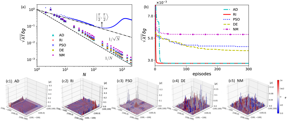
Figure 13: (a) The performance of the optimal probe states searched via AD (cyan triangles), RI (red pluses), PSO (blue crosses), DE (yellow circles) and NM (purple squares) in the Lipkin-Meshkov-Glick model in the absence of noise. The blue dots represents the value of $\sqrt{\lambda T}\delta g$ for the coherent spin state $|\pi/2,\pi/2\rangle$, and the dash-dotted black and dashed black lines represent $1/\sqrt{N}$ and $1/N$, respectively. (b) The convergence performance of AD (dash-dotted cyan line), RI (solid red line), PSO (dotted blue line), DE (dashed yellow line), and NM (dotted star purple line) in the case of $N=500$. (c1-c5) The searched optimal states with different algorithms in the case of $N=100$. The target time is chosen as $\lambda T=10$. The true value of $g$ is 0.5, and the value of $h/\lambda$ is set to be $0.1$. Planck units are applied here.

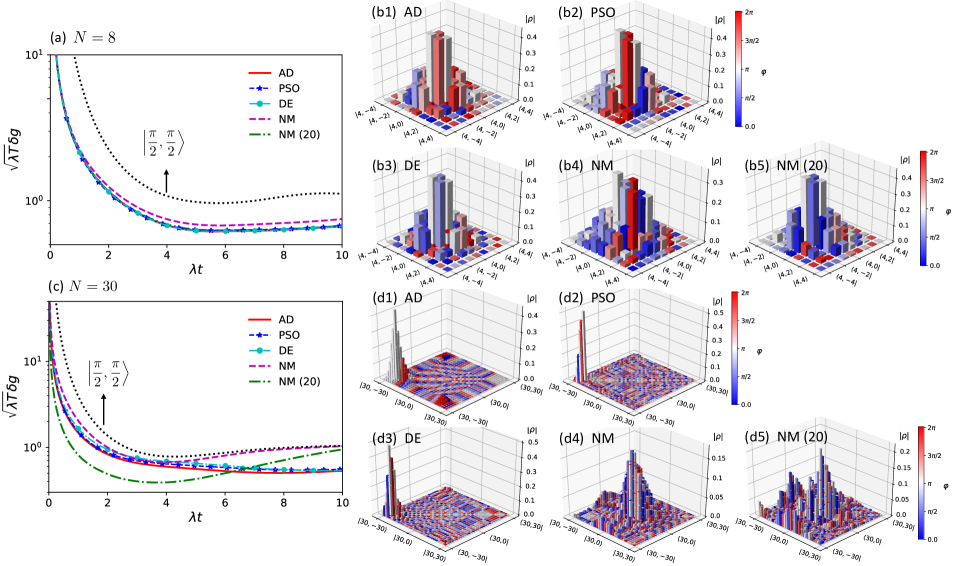
Figure 14: The performance of probe states obtained via different algorithms for (a) $N=8$ and (c) $N=30$ when the collective dephasing exists. The solid red line, dashed star blue line, dash-dotted circle cyan line, dashed purple line represent the values of $\sqrt{\lambda T}\delta g$ for the searched states obtained via AD, PSO, DE, and NM, respectively. The dash-dotted green line represents that of NM with 20 parallel sets. The dotted black line represent the result of $|\pi/2,\pi/2\rangle$. (b1-b5) The searched optimal states for $N=8$. (d1-d5) The searched optimal states for $N=30$. The target time $\lambda T=10$, and the true values of $g$ is 0.5. The value of $h/\lambda$ is set to be $0.1$ and the decay rate $\gamma/\lambda=0.1$. Planck units are applied here.

Apart from the aforementioned algorithms, there also exist dedicated algorithms for the state optimization in quantum parameter estimation. Here we introduce a reverse iterative algorithm (RI), which was first proposed in Refs. [117, 118] in the Bayesian estimation context, and then applied to the QFI in Ref. [119]. In the case of single-parameter estimation, the QFI can be rewritten into

$$\mathcal{F}_{aa}=\sup_{A}\left[2\mathrm{Tr}(A\partial_{a}\rho)-\mathrm{Tr}(\rho A^{2})\right].$$ (73)

This form is equivalent to the standard definition of the QFI as can be seen by solving the maximization problem $2\mathrm{Tr}(A\partial_{a}\rho)-\mathrm{Tr}(\rho A^{2})$ with respect to $A$, which is formally a quadratic function in matrix $A$ and the resulting extremum condition yields the standard linear equation for $\partial_{a}\rho=\frac{1}{2}(A\rho+\rho A)$, i.e., the optimal $A=L_{a}$ is just the SLD operator. When this solution is plugged into the formula and it yields $\mathrm{Tr}(\rho L^{2}_{a})$, which is in agreement with the standard definition of the QFI. Consider the parameterization process described by the Kraus operators given in Eq. (4), $\rho=\sum_{i}K_{i}(x)\rho_{0}K_{i}^{\dagger}(x)$. Taking into account Eq. (73), we see that the problem of identifying the optimal input state $\rho_{0}$ that maximizes the QFI, can be written as a double maximization problem,

$$\sup_{\rho_{0}}\mathcal{F}_{aa}=\sup_{A,\rho_{0}}\left[2\mathrm{Tr}(A\partial_{a}\rho)-\mathrm{Tr}(\rho A^{2})\right].$$ (74)

This observation leads to an effective iterative protocol, where for a fixed $\rho_{0}$ we find the optimal $A$ that maximizes the above expression, and then fixing the optimal $A$ found in the previous step we look for the optimal $\rho_{0}$. In order to implement the procedure, note that the QFI can be rewritten in the ‘Heisenberg picture’ form, where the Kraus operators effectively act on the $L_{a}$ operators, as

$$\mathcal{F}_{aa}=\mathrm{Tr}\left(\rho_{0}\mathcal{M}\right)$$ (75)

with

$$\mathcal{M}\!=\!\sum_{i}2\!\left[(\partial_{a}K^{\dagger}_{i})L_{a}K_{i}\!+\!K^{\dagger}_{i}L_{a}(\partial_{a}K_{i})\right]\!-\!K_{i}^{\dagger}L^{2}_{a}K_{i}.$$ (76)

This equation indicates that for a fixed $\mathcal{M}$ (i.e., fixed $A=L_{a}$), the optimal probe state is nothing but the eigenvector corresponding to the maximum eigenvalue of $\mathcal{M}$. The pseudocode of this algorithm is given in Algorithm 7. In one round of the optimization, $\mathcal{M}$ is calculated and its eigenvector with respect to the maximum eigenvalue of $\mathcal{M}$ is calculated and used as the probe state in the next round. In the package, this method can be invoked via method="RI". The number of episodes and the seed can be adjusted in **kwargs (shown in Table 3) via max_episode and seed. Notice that this method is only available when state.Kraus() is invoked, and in the current version of the package, it only works for the single-parameter quantum estimation, i.e., the objective function is the QFI. The extension to the CFI and the case of multiparameter estimation will be thoroughly discussed in an independent paper.

Example. Here we use the Lipkin-Meshkov-Glick model as an example to show the state optimization with QuanEstimation. The Hamiltonian of this model is [120]

$$H_{\mathrm{LMG}}=-\frac{\lambda}{N}(J_{1}^{2}+gJ_{2}^{2})-hJ_{3},$$ (77)

where $J_{i}=\frac{1}{2}\sum_{j=1}^{N}\sigma_{i}^{(j)}$ ($i=1,2,3$) is the collective spin operator with $\sigma_{i}^{(j)}$ the $i$th Pauli matrix for the $j$th spin. $N$ is the total number of spins, $\lambda$ is the spin-spin interaction strength, $h$ is the strength of the external field and $g$ is the anisotropic parameter. All searches with different algorithms start from the coherent spin state $|\theta=\pi/2,\phi=\pi/2\rangle$, which is defined by [121]

$$|\theta,\phi\rangle=\exp\left(-\frac{\theta}{2}e^{-i\phi}J_{+}+\frac{\theta}{2}e^{i\phi}J_{-}\right)|J,J\rangle,$$ (78)

where $|J,J\rangle$ is a Dicke state with $J=N/2$ and $J_{\pm}=J_{1}\pm iJ_{2}$. Here we consider the case that the search is constrained to pure states with fixed $J=N/2$, which can be expressed as $|\psi\rangle=\sum^{J}_{m=-J}c_{m}|J,m\rangle$ with $|J,m\rangle$ a general Dicke state and $c_{m}$ a complex coefficient. Let us first study the single-parameter scenario with $g$ the parameter to be estimated.

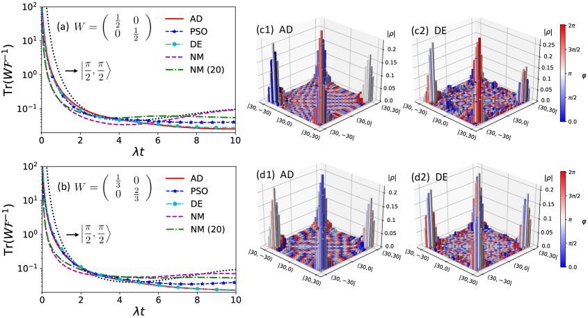
Figure 15: The performance of different algorithms for the weight matrix (a) $W=\mathrm{diag}(1/2,1/2)$ and (b) $W=\mathrm{diag}(1/3,2/3)$. The solid red line, dashed star blue line, dash-dotted circle cyan line, dashed purple line and dash-dotted green line represent the results obtained via AD, PSO, DE, NM, and NM with 20 parallel sets, respectively. The dotted black line represent the result of $|\pi/2,\pi/2\rangle$. (c1-c2) The optimal states obtained from AD and DE for $W=\mathrm{diag}(1/2,1/2)$. (d1-d2) The optimal states obtained from AD and DE for $W=\mathrm{diag}(1/3,2/3)$. The target time $\lambda T=10$. The true values of $g$ and $h/\lambda$ are set to be 0.5 and $0.1$. Planck units are applied here.

The performance of the optimal probe states searched via AD (cyan triangles), RI (red pluses), PSO (blue crosses), DE (yellow circles) and NM (purple squares) in the absence of noise are given in Fig. 13(a). Here $\delta g=1/\sqrt{\mathcal{F}_{gg}}$ is the theoretical optimal deviation for $g$. The target time is taken as $\lambda T=10$ (Planck units are applied). The performance of DDPG is not good enough and thus not shown in the figure. For a very small $N$, the searched optimal states do not show an obvious advantage than the state $|\pi/2,\pi/2\rangle$ (blue dots). However, when $N$ is large the advantage becomes significant, and the performance of all searched states outperform $|\pi/2,\pi/2\rangle$ and $1/\sqrt{N}$ (dash-dotted black line) in the case that $N$ is larger than around 6. For a large $N$, the performance of the states obtained via AD and RI are the best and very close to $1/N$ (dashed black line). The performance of DE and PSO basically coincide with each other (more accurately to say, the performance of DE is slightly better than that of PSO), but is worse than AD and RI. The performance of NM is the worst in this example. Please note that we cannot rashly say that the general performance of NM is worse than DE or PSO in the state optimization just based on this plot as different parameter settings in the algorithms sometimes could dramatically affect the behaviors, yet we basically use the general recommended settings in all algorithms. Nevertheless, different sensitivities of the parameter settings on the final result still indicates that DE and PSO are easier to locate optimal states than NM at least in this example.

Regarding the convergence performance in this example, as shown in Fig. 13(b), RI shows the fastest convergence speed and the best optimized value. AD is slightly slower than RI but still way faster than the gradient-free methods. However, the disadvantage of AD is that occupation of memory grows very fast with the increase of $N$. Hence, RI would be the best choice to try first for the state optimization in the case of unitary parameterization. In the last, as a demonstration, the searched optimal states via different algorithms in the case of $N=100$ are shown in Figs. 13(c1-c5).

Example. When the collective dephasing is involved, the dynamics of this system is governed by the following master equation

$$\partial_{t}\rho=-i[H_{\mathrm{LMG}},\rho]+\gamma\left(J_{3}\rho J_{3}-\frac{1}{2}\left\{\rho,J^{2}_{3}\right\}\right)$$ (79)

with $\gamma$ the decay rate. The performance of optimal probe states searched via AD (solid red line), PSO (dashed star blue line), DE (dash-dotted circle cyan line) and NM (dashed purple line) are illustrated with $N=8$ and $N=30$ in Figs. 14(a) and 14(c), respectively. The corresponding optimal probe states are given in Figs. 14(b1-b4) for $N=8$ and Figs. 14(d1-d4) for $N=30$. In both cases, the states obtained via AD, PSO and DE basically present coincidental performance at time $T$, and outperform $|\pi/2,\pi/2\rangle$ (dotted black lines). Similar to the unitary scenario, the state obtained via NM shows a worse performance at time $T$, and it even fails to find a better state than $|\pi/2,\pi/2\rangle$ in the case of $N=30$. In this figure, the number of parallel sets (also called particles in PSO and populations in DE) are 10 for all NM, DE and PSO. After increasing the number of parallel sets from 10 to 20 [labelled by NM (20) in the plot], the performance of NM (dash-dotted green line) improves in the case of $N=8$, which basically coincides with others. However, it still fails to find a better state when $N=30$. More number of parallel sets may be requires for NM in this case. The states obtained via NM (20) are shown in Figs. 14(b5) and 14(d5) for $N=8$ and $N=30$, respectively.

Algorithms	method=	**kwargs and default values
PSO	"PSO"	"p_num"	10
		"measurement0"	[]
		"max_episode"	[1000,100]
		"c0"	1.0
		"c1"	2.0
		"c2"	2.0
		"seed"	1234
DE	"DE"	"p_num"	10
		"measurement0"	[]
		"max_episode"	1000
		"c"	1.0
		"cr"	0.5
		"seed"	1234
AD	"AD"	"Adam"	False
(available when		"measurement0"	[]
mtype="input")		"max_episode"	300
		"epsilon"	0.01
		"beta1"	0.90
		"beta2"	0.99

Table 4: Available methods for measurement optimization in QuanEstimation and corresponding default parameter settings. Notice that AD is only available when mtype="input". Here measurement0 is the initial guess of the measurement.

Next we discuss the state optimization in multiparameter estimation. Consider the simultaneous estimation of $g$ and $h/\lambda$ in the Lipkin-Meshkov-Glick model with the dynamics in Eq. (79). Figures 15(a) and 15(b) show the performance of optimal states obtained via different algorithms for $W=\mathrm{diag}(1/2,1/2)$ and $W=\mathrm{diag}(1/3,2/3)$, respectively. In both cases AD (solid red line) and DE (dash-dotted circle cyan line) present the best performance at the target time $\lambda T=10$, and DE even slightly outperform AD in the case of $W=\mathrm{diag}(1/2,1/2)$. The performance of PSO (dashed star blue line) is worse than AD and DE, yet still better than NM (dashed purple line) and NM with 20 parallel sets (dash-dotted green line). The performance of NM does not even outperform the coherent spin state $|\pi/2,\pi/2\rangle$ (dotted black line) in the case of $W=\mathrm{diag}(1/2,1/2)$. Hence, apart from gradient-based algorithm like AD, PSO and DE would also be good choices for state optimizations. The optimal states obtained from AD and DE for $W=\mathrm{diag}(1/2,1/2)$ and $W=\mathrm{diag}(1/3,2/3)$ are demonstrated in Figs. 15(c1-c2) and Figs. 15(d1-d2), respectively. Although the performance on $\mathrm{Tr}(W\mathcal{F}^{-1})$ are basically the same for these states, they may still have gaps on other properties like the difficulties of preparation, the robustness to the imperfect preparation and so on. Hence, in practice one needs to compare these optimal states comprehensively case by case to make wise choices.

VIII Measurement optimization

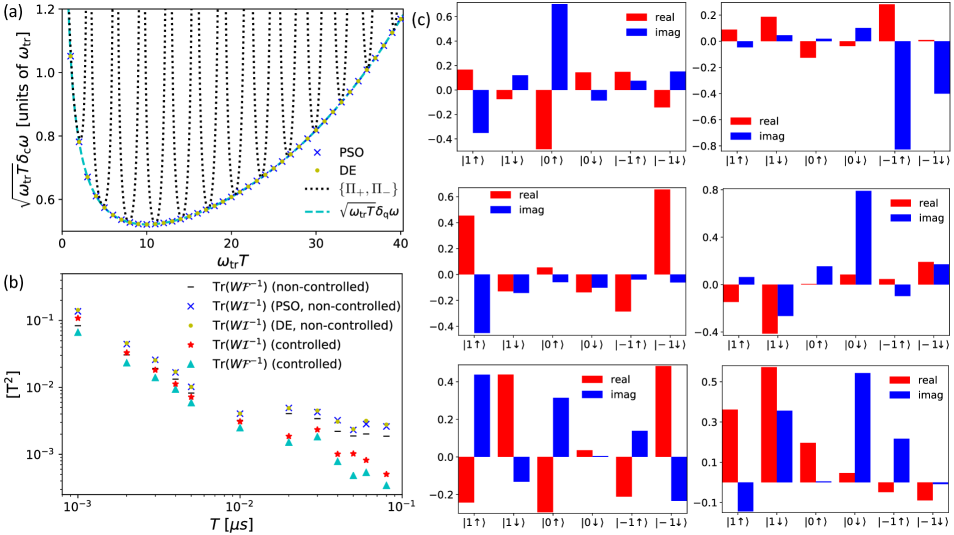
Figure 16: (a) The performance of optimal projective measurements obtained via PSO (blue crosses) and DE (yellow circles) in the case of single-parameter estimation. The dashed cyan line represents the values of $\sqrt{\omega_{\mathrm{tr}}T}\delta_{\mathrm{q}}\omega$ and the dotted black line represents the values of $\sqrt{\omega_{\mathrm{tr}}T}\delta_{\mathrm{c}}\omega$ with respect to the projective measurement $\{\Pi_{+}\!=\!|+\rangle\langle+|,\Pi_{-}\!=\!|-\rangle\langle-|\}$. The true value $\omega_{\mathrm{tr}}=1$. Planck units are applied in this plot. (b) The performance of optimal projective measurements obtained via PSO (blue crosses) and DE (yellow circles) in the case of multiparameter estimation in the absence of control. The black underlines and cyan triangles represent the values of $\mathrm{Tr}(W\mathcal{F}^{-1})$ without and with optimal control. The red pentagrams represent the controlled values of $\mathrm{Tr}(W\mathcal{I}^{-1})$ with the optimal measurements obtained in the non-controlled scenario. (c) Demonstration of the optimal projective measurement obtained by DE in the multiparameter estimation at the target time $T=0.04\,\mu$s. The red and blue bars represent the real and imaginary parts of the coefficients of the optimal measurement in the basis $\{|1\!\uparrow\rangle,|1\!\downarrow\rangle,|0\!\uparrow\rangle,|0\!\downarrow\rangle,|\!-\!1\!\uparrow\rangle,|\!-\!1\!\downarrow\rangle\}$.

Measurement is critical in quantum parameter estimation [122, 123, 124, 125]. On one hand, all asymptotic bounds require some optimal measurements to attain if it is attainable, and hence the search of optimal measurements is a natural requirement in theory to approach the ultimate precision limit. On the other hand, the choice of measurements is usually limited in practice, and how to find conditioned optimal measurements with the practical measurements in hand is an important step towards the design of a realizable scheme. QuanEstimation includes the optimization of measurements for several scenarios. The first one is the optimization of rank-one projective measurements. A set of projective measurements $\{\Pi_{i}\}$ satisfies $\Pi_{i}\Pi_{j}=\Pi_{i}\delta_{ij}$ and $\sum_{i}\Pi_{i}=\openone$, and it can be rewritten into $\{|\phi_{i}\rangle\langle\phi_{i}|\}$ with $\{|\phi_{i}\rangle\}$ an orthonormal basis in the Hilbert space. In this way, the optimization of rank-one projective measurement is equivalent to identifying the optimal basis, which can be realized using PSO and DE in QuanEstimation. In this case the automatic differentiation is not working very well due to the Gram-Schmidt orthogonalization procedure after the update of $\{|\phi_{i}\rangle\}$ according to the gradients. In some cases, the realizable measurement has to be limited in the linear combination of a given set of POVM, hence, the second scenario is to find the optimal linear combination of an input measurement. Moreover, in some cases the measurement $\{\Pi_{i}\}$ has to be fixed, but an arbitrary unitary operation can be invoked before performing the measurement, which is equivalent to a new measurement $\{U\Pi_{i}U^{\dagger}\}$. Based on this, the third scenario is to find the optimal rotated measurement of an input measurement.

The code in QuanEstimation for the execution of measurement optimization are as follows:

⬇

m = MeasurementOpt(mtype="projection",

minput=[],savefile=False,

method="DE",**kwargs)

m.dynamics(tspan,rho0,H0,dH,Hc=[],ctrl=[],

decay=[],dyn_method="expm")

m.CFIM(W=[])

In the case that the parameterization is described by the Kraus operators, replace m.dynamics() with the code m.Kraus(rho0,K,dK). The optimization method can be adjusted via method=" " and corresponding parameters can be set via **kwargs. The available optimization methods and corresponding default parameter settings are given in Table 4. dyn_method="ode" is also available here to invoke ODE for soloving the dynamics, except the case that method="AD" is applied. Two files "f.csv" and "measurements.csv" will be generated at the end of the program. When savefile=True, the measurements obtained in all episodes will be saved in "measurements.csv".

The variable mtype=" " defines the type of scenarios for the optimization, and currently it includes two options: mtype="projection" and mtype="input". The first one means the optimization is performed in the first scenario, i.e., within the set of projective measurements. In this case, minput=[] should keep empty. Since $|\phi_{i}\rangle$ in a rank-one projective measurement $\{|\phi_{i}\rangle\langle\phi_{i}|\}$ can be expended as $|\phi_{i}\rangle=\sum_{j}C_{ij}|j\rangle$ in a given orthonormal basis $\{|j\rangle\}$, the optimization of the rank-one projective measurement is equivalent to the optimization of a complex matrix $C$. When the gradient-free methods are applied, all entries in $C$ are updated via the given algorithm in each episode, then adjusted via the Gram-Schmidt orthogonalization procedure to make sure $\{|\phi_{i}\rangle\langle\phi_{i}|\}$ is a legitimate projective measurement, i.e., $\langle\phi_{i}|\phi_{j}\rangle=\delta_{ij},\leavevmode\nobreak\ \forall i,j$ and $\sum_{i}|\phi_{i}\rangle\langle\phi_{i}|=\openone$. The second option mtype="input" means the optimization is performed in the second and third scenarios. The input rule of minput for the second scenario is minput=["LC", [Pi1,Pi2,…], m] and for the third one is minput=["rotation", [Pi1,Pi2,…]]. Here [Pi1,Pi2,…] is a list of matrices representing the input measurement $[\Pi_{1},\Pi_{2},\dots]$. The variable m in the second scenario is an integer representing the number of operators of the output measurement, and thus should be no larger than that of the input measurement. For example, assume the input measurement is $\{\Pi_{i}\}^{6}_{i=1}$ and input 4 in the position of m means the the output measurement is $\{\Pi^{\prime}_{i}\}^{4}_{i=1}$ where $\Pi^{\prime}_{i}=\sum^{6}_{j=1}B_{ij}\Pi_{j}$. The optimization is to find an optimal real matrix $B$ for the optimal CFI or $\mathrm{Tr}(W\mathcal{I}^{-1})$. To make sure the updated measurement in each episode is still a legitimate POVM, all entries of $B$ are limited in the regime $[0,1]$ and $\sum_{i}B_{ij}$ is required to be 1, which is realized by the normalization process. In this scenario, apart from PSO and DE, AD can also be implemented. In the third scenario, the unitary operation is expressed by $U=\prod_{k}\exp(is_{k}\lambda_{k})$ where $\lambda_{k}$ is a SU($N$) generator and $s_{k}$ is a real number in the regime $[0,2\pi]$. The optimization is to find an optimal set of $\{s_{k}\}$ for the optimal CFI or $\mathrm{Tr}(W\mathcal{I}^{-1})$, and similar to the second scenario, AD is also available here besides PSO and DE. In the case that mtype="projection", each entry of measurement0 in **kwargs is a list of arrays, and in the case that mtype="input", each entry is an array.

Example. Now we consider two models to demonstrate the measurement optimizations in the first scenario. The first one is a single-parameter case with the single-qubit Hamiltonian $H=\omega\sigma_{3}/2$ and dynamics in Eq. (12). $\delta_{\mathrm{c}}\omega$ and $\delta_{\mathrm{q}}\omega$ are defined in Eqs. (56) and (57). As shown in Fig. 16(a), $\delta_{\mathrm{c}}\omega$ for the projective measurement $\{\Pi_{+}\!=\!|+\rangle\langle+|,\Pi_{-}\!=\!|-\rangle\langle-|\}$ (dotted black line) can only reach $\delta_{\mathrm{q}}\omega$ (dashed cyan line) at some specific time points, which has already been shown in Sec. IV.1. However, utilizing the optimal projective measurements obtained via PSO (blue crosses) and DE (yellow circles), $\delta_{\mathrm{c}}\omega$ saturates $\delta_{\mathrm{q}}\omega$ for all target time. This performance coincides with the common understanding that the QFI can be theoretically attained by certain optimal measurements.

In the case of multiparameter estimation, we use the Hamiltonian in Eq. (63) and dynamics in Eq. (72) to demonstrate the performance of the optimal projective measurements. The magnetic field $\vec{B}$ is still the quantity to be estimated. Different with the single-parameter case, the values of $\mathrm{Tr}(W\mathcal{I}^{-1})$ for the optimal measurements found by PSO (blue crosses) and DE (yellow circles) cannot attain $\mathrm{Tr}(W\mathcal{F}^{-1})$ (black underlines) in the absence of control, as shown in Fig. 16(b). The gap between $\mathrm{Tr}(W\mathcal{F}^{-1})$ and $\mathrm{Tr}(W\mathcal{I}^{-1})$ is due to the fact that the quantum Cramér-Rao bound is not attainable here. Next, together with the optimal measurement which gives the lowest $\mathrm{Tr}(W\mathcal{I}^{-1})$, the control is also invoked to further evaluate the reduction of $\mathrm{Tr}(W\mathcal{I}^{-1})$. Utilizing the optimal controls obtained via auto-GRAPE, the values of $\mathrm{Tr}(W\mathcal{I}^{-1})$ (red pentagrams) continue to reduce compared to the non-controlled case, yet it is still unable to attain the controlled values of $\mathrm{Tr}(W\mathcal{F}^{-1})$ (cyan triangles) in general due to the attainability problem. Nevertheless, their differences are very insignificant for some target time, indicating that the combined performance of the optimal measurement and optimal control approaches to the ultimate precision limit. The optimal measurement $\{|\phi_{1}\rangle\langle\phi_{1}|,\cdots,|\phi_{6}\rangle\langle\phi_{6}|\}$ obtained by DE in the absence of control are demonstrated in Fig. 16(c). The red and blue bars represent the real and imaginary parts of the coefficients of $|\phi_{1}\rangle$ to $|\phi_{6}\rangle$ in the basis $\{|1\!\uparrow\rangle,|1\!\downarrow\rangle,|0\!\uparrow\rangle,|0\!\downarrow\rangle,|\!-\!1\!\uparrow\rangle,|\!-\!1\!\downarrow\rangle\}$.

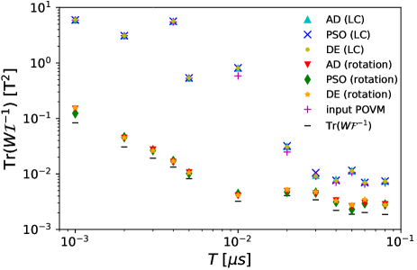
Figure 17: Demonstration of the measurement optimization in the second (LC) and third scenarios (rotation). The cyan upward triangles, blue crosses and yellow circles represent the performance of optimal measurements found by AD, PSO, and DE, respectively in the second scenario. The red downward triangles, green diamonds and orange pentagrams represent the performance of optimal measurements found by AD, PSO, and DE in the third scenario.

The optimizations in the second and third scenarios are also demonstrated with the Hamiltonian in Eq. (63) and dynamics in Eq. (72). The input measurement is taken as $\{|ij\rangle\langle ij|\}_{i=0,\pm 1;j=\uparrow,\downarrow}$, which includes 6 operators. In the second scenario, the number of output POVM operators is set to be 4. As shown in Fig. 17, the performance of measurements found by AD (cyan upward triangles), PSO (blue crosses) and DE (yellow circles) approach to and even reach that of the input measurement (magenta pluses). This fact indicates that in this case, an optimal 4-operator measurement can reach the performance of the original 6-operator measurement, and the reduction of operator numbers may benefit the practical precision of the measurements in experiments. In the third scenario, the performance of optimal measurements found by AD (red downward triangles), PSO (green diamonds), and DE (orange pentagrams) not only significantly better than that of the input measurement, but also approach to the ultimate precision limit given by $\mathrm{Tr}(W\mathcal{F}^{-1})$ (black underlines), indicating that the performance of these optimal measurements are very close to that of the global optimal measurements, if there exist any. The probe states, the true values of the parameters to be estimated and other parameters are set to be the same with those in Sec. VI.7.

IX Comprehensive optimization

Algorithms	method=	**kwargs and default values
PSO	"PSO"	"p_num"	10
		"psi0"	[]
		"ctrl0"	[]
		"measurement0"	[]
		"max_episode"	[1000,100]
		"c0"	1.0
		"c1"	2.0
		"c2"	2.0
		"seed"	1234
DE	"DE"	"p_num"	10
		"psi0"	[]
		"ctrl0"	[]
		"measurement0"	[]
		"max_episode"	1000
		"c"	1.0
		"cr"	0.5
		"seed"	1234
AD	"AD"	"Adam"	False
(available		"psi0"	[]
for SC)		"ctrl0"	[]
		"measurement0"	[]
		"max_episode"	300
		"epsilon"	0.01
		"beta1"	0.90
		"beta2"	0.99

Table 5: Available methods for comprehensive optimization in QuanEstimation and corresponding default parameter settings. Notice that AD is only available when com.SC() is called.

Figure 18: Illustration of the comprehensive optimization (first lines with gray background) and combination of univariate optimizations (second lines) in four types of multivariate optimizations, including the optimizations of (a) the probe state and measurement (SM), (b) the probe state and control (SC), (c) control and measurement (CM), and (d) the probe state, control, and measurement (SCM).

The previous sections focused on the univariate (single variable) optimizations. However, in a practical scenario the probe state, control (if available) and measurement may all need to be optimized. More importantly, the optimal results obtained for an univariate optimization may cease to be optimal when other variables are involved. For example, the optimal probe state and measurement for the non-controlled case may not be optimal anymore in the controlled case. Hence, sometimes a comprehensive optimization, i.e., simultaneous multivariate optimization, is in need.

QuanEstimation can deal with four types of multivariate optimizations, including the optimizations of the probe state and measurement (SM), the probe state and control (SC), control and measurement (CM), and all three together (SCM). In these scenarios, the key feature of comprehensive optimization is that all variables are optimized simultaneously. Regarding the objective function, in the cases of SM, CM, and SCM, namely, when the measurement is involved, it has to be dependent on the measurement. In current version of the package it is chosen as the CFI or $\mathrm{Tr}(W\mathcal{I}^{-1})$. In the case of SC, the objective function could be either QFI/$\mathrm{Tr}(W\mathcal{F}^{-1})$ or CFI/$\mathrm{Tr}(W\mathcal{I}^{-1})$ for a flexible or fixed choice of measurement. The process of comprehensive optimizations and corresponding objective functions have been illustrated in the first lines (with gray background) in Figs. 18(a-d). In QuanEstimation, the code for the execution of comprehensive optimization are:

⬇

com = ComprehensiveOpt(savefile=False,

method="DE",**kwargs)

com.dynamics(tspan,H0,dH,Hc=[],ctrl=[],

decay=[],ctrl_bound=[],

dyn_method="expm")

com.SM(W=[])

com.SC(W=[],M=[],target="QFIM",LDtype="SLD")

com.CM(rho0,W=[])

com.SCM(W=[])

In the case that the parameterization is described by the Kraus operators, replace com.dynamics() with the code com.Kraus(K,dK). All four types of comprehensive optimizations can be called through com.SM(), com.SC(), com.CM(), and com.SCM(). Notice that if com.Kraus() is invoked, only com.SM() is available as control is not suitable for the parameterization process described by the Kraus operators. In com.CM(), the input rho0 is a matrix representing the fixed probe state. In com.SC(), the objective function can be set via target=" ", including three choices target="QFIM" (default), target="CFIM", and target="HCRB". If a set of measurement is input via M=[], the objective function will be automatically chosen as the CFIM regardless of the input in target=" ". The type of QFIM can be adjusted via LDtype=" " ("SLD", "RLD", "LLD"). The available methods for the comprehensive optimization and corresponding default parameter settings are given in Table 5. Notice that AD is only available when com.SC() is called and the objective function is not the HCRB. At the end of the program, "f.csv" will be generated including the values of the objective function in all episodes. In the meantime, some or all of the files "controls.csv", "states.csv", and "measurements.csv" will also be generated according to the type of comprehensive optimization.

Alternatively, the multivariate optimization can also be finished by the combination of univariate optimizations, as shown in the second lines in Figs. 18(a-d). In the case of SM (or CM) shown in Fig. 18(a) [Fig. 18(c)], one could first perform the state (control) optimization with QFI/$\mathrm{Tr}(W\mathcal{F}^{-1})$ the objective function. Next, take the found optimal state (control) as the fixed input, and further optimize the measurement with CFI/$\mathrm{Tr}(W\mathcal{I}^{-1})$ the objective function. If the optimized values of the CFI/$\mathrm{Tr}(W\mathcal{I}^{-1})$ in the second process reaches the optimized values of the QFI/$\mathrm{Tr}(W\mathcal{F}^{-1})$ in the first process, the entire scheme is then optimal. Things could be more complex in the multiparameter estimation due to the attainability problem. The existence of the gap between the optimized $\mathrm{Tr}(W\mathcal{I}^{-1})$ and $\mathrm{Tr}(W\mathcal{F}^{-1})$ does not necessarily mean the scheme is not optimal. Nevertheless, there is no doubt that a smaller gap always implies a better scheme at least in theory. In the case of SC, the state optimization and control optimization can be performed in turn with the optimal quantity found in the previous turn as the fixed input [Fig. 18(b)]. Same with the comprehensive optimization, both QFI/$\mathrm{Tr}(W\mathcal{F}^{-1})$ and CFI/$\mathrm{Tr}(W\mathcal{I}^{-1})$ can be taken as the objective function in this case. At last, in the case of SCM the combination strategy in SC could be performed first with QFI/$\mathrm{Tr}(W\mathcal{F}^{-1})$ the objective function, and the measurement is further optimized with the found optimal state and control as the fixed input [Fig. 18(d)]. Same with the scenario of SM, if the optimized CFI/$\mathrm{Tr}(W\mathcal{I}^{-1})$ obtained in the second process reaches the optimized QFI/$\mathrm{Tr}(W\mathcal{F}^{-1})$ in the first process, the entire scheme is optimal.

Example. Now we provide some demonstrations on the comprehensive optimization with QuanEstimation and compare their performance with the combination strategy. First, consider a non-controlled example with the single-qubit Hamiltonian $\omega\sigma_{3}/2$, which is a SM scenario. The dynamics is governed by Eq. (12) with decay rates $\gamma_{-}/\omega_{\mathrm{tr}}=0$ and $\gamma_{+}/\omega_{\mathrm{tr}}=0.1$. The target time $\omega_{\mathrm{tr}}T=20$. In this case, the optimized values of $\sqrt{\omega_{\mathrm{tr}}T}\delta_{\mathrm{c}}\omega$ in the comprehensive optimization and combination strategy are both 0.608 (in the units of $\omega_{\mathrm{tr}}$, same below), equivalent to the optimal $\sqrt{\omega_{\mathrm{tr}}T}\delta_{\mathrm{q}}\omega$ obtained in the solely state optimization, indicating that the schemes found by both strategies are indeed optimal in theory. Next we invoke the controls described in Eq. (45). In the case of SC, the optimized $\sqrt{\omega_{\mathrm{tr}}T}\delta_{\mathrm{q}}\omega$ obtained in the combination strategy is 0.441, and that in the comprehensive optimization is 0.440. Furthermore, in the case of SCM, the optimized $\sqrt{\omega_{\mathrm{tr}}T}\delta_{\mathrm{c}}\omega$ provided by the combination strategy is 0.441, equivalent to the optimal $\sqrt{\omega_{\mathrm{tr}}T}\delta_{\mathrm{q}}\omega$ obtained in the SC, and that provided by the comprehensive optimization is 0.443. The performance of these two strategies basically coincide with each other in this example.

This equivalent performance may due to two facts: the example is simple and the QFI is attainable in theory. In the multiparameter estimation, these two strategies may show divergent performance as the QFIM is not always guaranteed to be attainable. For example, in the case of SCM, $\mathrm{Tr}(W\mathcal{F}^{-1})$ are first optimized in the SC. However, it is hard to say whether the optimal probe state and control for an unattainable $\mathrm{Tr}(W\mathcal{F}^{-1})$ can still provide a good $\mathrm{Tr}(W\mathcal{I}^{-1})$ and benefit the subsequent measurement optimization. To investigate it, we still take the nitrogen-vacancy center as an example. The free Hamiltonian, control Hamiltonian, and dynamics are described in Eqs. (63), (71), and (72). The performance of comprehensive optimization and combination strategy in the SCM are shown in Fig. 19. The comprehensive optimization (dashed blue line), which takes $\mathrm{Tr}(W\mathcal{I}^{-1})$ as the objective function, basically converges at around $110$ episodes. The combination strategy (solid red line) splits into two parts, the one in the first 500 episodes is the combination optimization of SC, and that in the last 500 episodes is the optimization of the measurement. The gap between these two lines is actually the gap between the optimal $\mathrm{Tr}(W\mathcal{F}^{-1})$ and the value of $\mathrm{Tr}(W\mathcal{I}^{-1})$ with a random measurement. In the SC part, the alternative optimizations of the probe state and control can be done in different ways due to the episode number of each optimization. As shown in the inset of Fig. 19, here we test several selections, including 20 episodes for each optimization (solid circle blue line), 50 episodes for each optimization (dashed green line), 100 episodes for each optimization (dash-dotted cyan line), 200 episodes for state optimization and 300 episodes for control optimization (solid red line), and 300 episodes for state optimization and 200 episodes for control optimization (dotted black line). In these selections, the fourth one, 200 episodes for state optimization and 300 episodes for control optimization, shows the best performance at the end of the 500 episodes, and the corresponding optimal state and control are chosen for the subsequent measurement optimization. In this example, the final performance of the combination strategy is better than that of the simultaneous strategy, indicating that the unattainability of $\mathrm{Tr}(W\mathcal{F}^{-1})$ in the SC does not present negative effects on the final performance. However, this result does not mean the combination strategy is always better in general. In practice, the comparison of these two strategies might still be needed case by case in the scheme design.

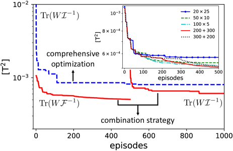
Figure 19: Performance comparison between the comprehensive optimization and combination strategy in the multiparameter estimation in the case of SCM. The dashed blue line represents the optimization of $\mathrm{Tr}(W\mathcal{I}^{-1})$ in the comprehensive optimization. The solid red lines represent the optimization of $\mathrm{Tr}(W\mathcal{F}^{-1})$ in the SC (first 500 episodes) and that of $\mathrm{Tr}(W\mathcal{I}^{-1})$ in the measurement optimization (last 500 episodes) in the combination strategy. The inset shows the performance of different combination strategies in the SC part due to the episode number of each optimization. All the optimizations in the figure are finished by DE.

X Adaptive measurement schemes

Adaptive measurement is another common scenario in quantum parameter estimation. In this scenario, apart from the unknown parameters $\mathbb{x}$, the Hamiltonian also includes a set of tunable parameters $\mathbb{u}$. A typical case is that the tunable parameters are invoked by the same way with $\mathbb{x}$, resulting in the total Hamiltonian $H(\mathbb{x}+\mathbb{u})$. In the point estimation approach, the QFIM and CFIM computed at the true values of $\mathbb{x}$ may not always provide the practically achievable precision due to the fact that the actual working point may be slightly away from the true values. Hence, the tunable parameters $\mathbb{u}$ are invoked to let the Hamiltonian $H(\mathbb{x}+\mathbb{u})$ work at the optimal point $\mathbb{x}_{\mathrm{opt}}$. An obvious difficulty for the implementation of this scheme is that one actually does not known the true values in practice, which means $\mathbb{u}$ has to be given according to the estimated values $\hat{\mathbb{x}}$, and the entire scheme would only be useful when it is implemented adaptively. In the meantime, a pre-estimation of $\mathbb{x}$ is usually needed. The inaccuracy of $\hat{\mathbb{x}}$ would result in the inaccuracy of $\mathbb{u}$, and $\hat{\mathbb{x}}+\mathbb{u}$ is then inevitably far from $\mathbb{x}_{\mathrm{opt}}$, causing a lousy performance of the scheme. This scheme has been demonstrated by Berni et al. [126] in optical phase estimation with additional real-time feedback controls.

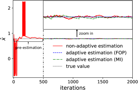
Figure 20: Performance comparison between the adaptive schemes realized by FOP (dashed blue line) and MI (dash-dotted green line), and the non-adaptive schemes (solid red line). The adaptive measurement starts after 500 rounds of pre-estimation. The non-adaptive scheme is a full Bayesian estimation. The dotted black line represents the true value.

Now let us introduce in detail all steps required to implement this scheme. Consider the Hamiltonian $H(\mathbb{x})$ where $\mathbb{x}$ is restricted in a finite regime with a prior distribution $p(\mathbb{x})$. The first step is to find the optimal value $\mathbb{x}_{\mathrm{opt}}$ in this regime with respect to the minimum $\mathrm{Tr}(W\mathcal{I}^{-1})$ when the measurement is fixed. If the measurement can be altered flexibly in practice, $\mathbb{x}_{\mathrm{opt}}$, together with the corresponding optimal measurement, can be obtained with $\mathrm{Tr}(W\mathcal{F}^{-1})$ the objective function. Next, perform the pre-estimation via the Bayesian estimation with the fixed or optimal measurement and update the prior distribution with the posterior distribution in Eq. (21). When $p(\mathbb{x})$ has been updated to a reasonable narrow distribution, the tunable parameters $\mathbb{u}$ are then invoked into the system. In the $n$th round of this step, with the observed result $y^{(n)}$, the posterior distribution is obtained via the Bayes’ rule as

$$p(\mathbb{x},\mathbb{u}^{(n)}|y^{(n)})=\frac{p(y^{(n)}|\mathbb{x},\mathbb{u}^{(n)})p(\mathbb{x})}{\int p(y^{(n)}|\mathbb{x},\mathbb{u}^{(n)})p(\mathbb{x})\mathrm{d}\mathbb{x}},$$ (80)

where $\mathbb{u}^{(n)}$ is obtained in the $(n-1)$th round. The estimated value $\hat{\mathbb{x}}^{(n)}$ can be obtained through the MAP, $\hat{\mathbb{x}}^{(n)}=\mathrm{argmax}\,p(\mathbb{x},\mathbb{u}^{(n)}|y^{(n)})$. The value of $\mathbb{u}$ used in the next round is obtained by $\mathbb{u}^{(n+1)}=\mathbb{x}_{\mathrm{opt}}-\hat{\mathbb{x}}^{(n)}$, and the prior distribution is also replaced by the current posterior distribution. This update method of $\mathbb{u}$ is referred to as the fixed optimal point method (FOP) in this paper. In QuanEstimation, the pre-estimation can be finished with the function Bayes() discussed in Sec. IV.4, and the adaptive process can be executed with the code:

⬇

apt = Adapt(x,p,rho0,method="FOP",

savefile=False,max_episode=1000,

eps=1e-8)

apt.dynamics(tspan,H,dH,Hc=[],ctrl=[],

decay=[],dyn_method="expm")

apt.CFIM(M=[],W=[])

In the case that the parameterization process is described by the Kraus operators, replace apt.dynamics() with apt.Kraus(K,dK). The inputs x and p are the same with those in Bayes(). The input H is a list of matrices representing the Hamiltonian with respect to the values in x, and it is multidimensional in the multiparameter case. dH is a (multidimensional) list with each entry also a list representing $\partial_{\mathbb{x}}H$ with respect to the values in x. In the case that specific functions of $H$ and $\partial_{\mathbb{x}}H$ can be provided, H and dH can be alternatively generated via the function BayesInput() discussed in Sec. III. In apt.CFIM(), M is the input measurement and the default one is a set of SIC-POVM.

During the running of the code, three files "xout.csv", "y.csv", and "pout.csv" will be generated including the data of $\hat{\mathbb{x}}$, result $y$ in all rounds of iteration and final obtained $p(\mathbb{x})$. In the case that savefile=True, "pout.csv" contains the data of $p(\mathbb{x})$ in all rounds. If the choice of measurement is flexible in the experiment, before the invocation of apt.CFIM(), the optimal measurement with respect to $\mathbb{x}_{\mathrm{opt}}$ can be first obtained via calling M = apt.Mopt(W=[]). In the case that the users would like to run the pre-estimation with the optimal measurement, they can just call apt.Mopt() first and input the optimal measurement to Bayes() for the pre-estimation.

During the running of apt.CFIM(), the users should type the result $y$ obtained in practice on the screen and receive the values of $\mathbb{u}$ used for the next round of experiment. In the case that the users have already done the pre-estimation by themselves, they can directly use Adapt() without calling Bayes() first.

Apart from the FOP, $\mathbb{u}$ can also be updated via other strategies. One such choice is utilizing the optimization of the mutual information (MI), which is defined by

$$I(\mathbb{u})\!=\!\int\!p(\mathbb{x})\sum_{y}p(y|\mathbb{x},\mathbb{u})\mathrm{log}_{2}\!\left[\frac{p(y|\mathbb{x},\mathbb{u})}{\int p(\mathbb{x})p(y|\mathbb{x},\mathbb{u})\mathrm{d}\mathbb{x}}\right]\!\mathrm{d}\mathbb{x}.$$ (81)

In the $n$th round, the prior distribution $p(\mathbb{x})$ is updated via Eq. (80), and $\mathbb{u}^{(n+1)}$ is obtained by the equation $\mathbb{u}^{(n+1)}=\mathrm{argmax}\leavevmode\nobreak\ I(\mathbb{u})$. In QuanEstimation, this method can be invoked by setting method="MI" in Adapt(). Notice that in this method a good pre-estimation should let the prior distribution converges to zero at the boundary of the input x.

Let us still take the Hamiltonian in Eq. (22) as an example. The initial state is $|+\rangle$ and the target time $\omega_{0}T=1$ (Planck units are applied). The prior distribution is uniform in the regime $(-\pi/4,3\pi/4)$. In this regime, zero is an optimal point and is chosen to be $x_{\mathrm{opt}}$. The measurement is $\{|+\rangle\langle+|,|-\rangle\langle-|\}$. The results are simulated by generating random values in the regime $[0,1]$. When it is smaller (larger) than $p(+|x)$, the posterior distribution is calculated with $p(+|x)$ [$p(-|x)$]. As shown in Fig. 20, after 500 rounds of pre-estimation, the adaptive schemes realized by FOP (dashed blue line) and MI (dash-dotted greeen line) indeed show better performance, namely, smaller variance, compared to the non-adaptive scheme (solid red line) which is fully finished by the Bayesian estimation. Notice that this figure is only a one-time simulation of the experiment. The performance may be different when the results are different.

Another famous adaptive scheme is the online adaptive phase estimation, proposed by Berry et al. [127, 128], in the scenario of Mach-Zehnder interferometer (MZI). In this scheme, after reading the result $y^{(n)}$ in the $n$th round, the value of the tunable phase $\Phi_{n+1}$ or phase difference $\Delta\Phi_{n+1}$ is generated. The relation between $\Phi_{n+1}$ and $\Delta\Phi_{n+1}$ can be taken as $\Phi_{n+1}=\Phi_{n}-(-1)^{y^{(n)}}\Delta\Phi_{n+1}$. Hentschel and Sanders [72, 73] further provided an offline strategy with PSO, and the optimization methods are further extended to DE [75] and genetic algorithm [129] in recent years. Apart from the original references, details of this scheme can also be found in a recent review [17]. In QuanEstimation, this scheme can be executed by the code:

⬇

apt = Adapt_MZI(x,p,rho0)

apt.general()

apt.online(target="sharpness",output="phi")

The input rho0 is a matrix representing the probe state. The output can be tuned between $\Phi$ and $\Delta\Phi$ by setting output="phi" or output="dphi" in apt.online() in the demonstrating code. target="sharpness" means the tunable phase is obtained by the maximization of the sharpness function. The specific formula of the sharpness function can be found in Refs. [127, 128, 72, 73, 17]. Alternatively, the sharpness function can also be replaced by the mutual information in Eq. (81) via setting target="MI", which has been both theoretically and experimentally discussed by DiMario and Becerra in 2020 [130].

The offline strategy can also be executed by replacing apt.online() with the code:

⬇

apt.offline(target="sharpness",method="DE",

**kwargs)

PSO is also available here (method="PSO"). When the entire program is finished, a file named "xout.csv" including the data of output in all rounds will be generated. In the case of online scheme, an additional file "y.csv" including the result $y$ in all rounds will also be generated. The design of apt.general() here is to give us a space for the further inclusion of the adaptive phase estimation in other optical scenarios such as the SU(1,1) interferometers.

XI Summary

In this paper, we present a new open-source toolkit, QuanEstimation, for the design of optimal schemes in the quantum parameter estimation. The source of the package, as well as the demonstrating code for the calculation of all examples discussed in this paper, can be download in GitHub [131] and the documentation is in Ref. [132]. This package is based on both platforms of Python and Julia. The combined structure is to guarantee the calculation efficiency of Julia is fully utilized, and in the meantime, the people who have no knowledge of Julia would have no obstacle in using this package. In the meantime, a full Julia version of the package is also available in GitHub [133], which is suitable for those familiar with Julia. QuanEstimation includes several well-studied metrological tools in quantum parameter estimation, such as the various types of Cramér-Rao bounds and their quantum correspondences, quantum Ziv-Zakai bound, and Bayesian estimation. To perform the scheme design, QuanEstimation can execute the optimizations of the probe state, control, measurement, and the comprehensive optimizations, namely, the simultaneous optimizations among them. General adaptive measurement schemes as well as the adaptive phase estimation can also be performed with this toolkit.

QuanEstimation is suitable for many practical quantum systems, especially those with finite-dimensional Hilbert spaces, such as the trapped ions, nitrogen-vacancy centers, and quantum circuits. Therefore, it is not only useful for the theorists working in the field of quantum parameter estimation, but could also be particularly useful for the experimentalists who are not familiar with the theories in this field yet intend to utilize them to design experimental schemes. More functions and features will be constantly input into the package and the calculation efficiency for certain specific scenarios will be further improved in the future. Moreover, the calculations in QuanEstimation are majorly based on the density matrices, which may cause inefficiency when the dimension of Hilbert space is large. More technologies targeting at the many-body systems, such as the sparse matrices and matrix product states, will be further involved in the package in the future. We believe that there is a good chance that this package would become a common toolkit in the field of quantum metrology for the numerical calculations and scheme designs.

- [1] V. Giovannetti, S. Lloyd, and L. Maccone, Quantum-Enhanced Measurements: Beating the Standard Quantum Limit, Science 306, 1330-1336 (2004).
- [2] V. Giovannetti, S. Lloyd, and L. Maccone, Advances in quantum metrology, Nat. Photon. 5, 222-229 (2011).
- [3] C. L. Degen, F. Reinhard, and P. Cappellaro, Quantum sensing, Rev. Mod. Phys. 89, 035002 (2017).
- [4] D. Braun, G. Adesso, F. Benatti, R. Floreanini, U. Marzolino, M. W. Mitchell, and S. Pirandola, Quantum-enhanced measurements without entanglement, Rev. Mod. Phys. 90, 035006 (2018).
- [5] L. Pezzè, A. Smerzi, M. K. Oberthaler, R. Schmied, and P. Treutlein, Quantum metrology with nonclassical states of atomic ensembles, Rev. Mod. Phys. 90, 035005 (2018).
- [6] The LIGO Scientific Collaboration, Enhanced sensitivity of the LIGO gravitational wave detector by using squeezed states of light, Nat. Photon. 7, 613-619 (2013).
- [7] K. M. Backes et al., A quantum enhanced search for dark matter axions, Nature 590, 238-242 (2021).
- [8] M. Jiang, H. Su, A. Garcon, X. Peng, and D. Budker, Search for axion-like dark matter with spin-based amplifiers, Nat. Phys. 17, 1402-1407 (2021).
- [9] C. W. Helstrom, Minimum mean-squared error of estimates in quantum statistics, Phys. Lett. A 25, 101-102 (1967).
- [10] M. G. A. Paris, Quantum estimation for quantum technology, Int. J. Quantum Inf. 7, 125 (2009).
- [11] G. Tóth and I. Apellaniz, Quantum metrology from a quantum information science perspective, J. Phys. A: Math. Theor. 47, 424006 (2014).
- [12] M. Szczykulska, T. Baumgratz, and A. Datta, Multi-parameter quantum metrology, Adv. Phys. X 1, 621-639 (2016).
- [13] J. Liu, H. Yuan, X.-M. Lu, and X. Wang, Quantum Fisher information matrix and multiparameter estimation, J. Phys. A: Math. Theor. 53, 023001 (2020).
- [14] R. Demkowicz-Dobrzański, W. Górecki, and M. Guţă, Multi-parameter estimation beyond Quantum Fisher Information, J. Phys. A: Math. Theor. 53, 363001 (2020).
- [15] J. S. Sidhu and P. Kok, Geometric perspective on quantum parameter estimation, AVS Quantum Sci. 2, 014701 (2020).
- [16] F. Albarelli, M. Barbieri, M. G. Genoni, and I.Gianani, A perspective on multiparameter quantum metrology: From theoretical tools to applications in quantum imaging, Phys. Lett. A 384, 126311 (2020).
- [17] J. Liu, M. Zhang, H. Chen, L. Wang, and H. Yuan, Optimal Scheme for Quantum Metrology, Adv. Quantum Technol. 5, 2100080 (2022).
- [18] V. Erol, F. Ozaydin, and A. Altintas, Analysis of Entanglement Measures and LOCC Maximized Quantum Fisher Information of General Two Qubit Systems, Sci. Rep. 4, 5422 (2014).
- [19] J. R. Johansson, P. D. Nation, and F. Nori, QuTiP: An open-source Python framework for the dynamics of open quantum systems, Comp. Phys. Comm. 183, 1760 (2012).
- [20] J. R. Johansson, P. D. Nation, and F. Nori, QuTiP 2: A Python framework for the dynamics of open quantum systems, Comp. Phys. Comm. 184, 1234 (2013).
- [21] S. Machnes, U. Sander, S. J. Glaser, P. de Fouquières, A. Gruslys, S. Schirmer, and T. Schulte-Herbrüggen, Comparing, optimizing, and benchmarking quantum-control algorithms in a unifying programming framework, Phys. Rev. A 84, 022305 (2011).
- [22] H. J. Hogben, M. Krzystyniak, G. T. P. Charnock, P. J. Hore, and I. Kuprov, Spinach-A software library for simulation of spin dynamics in large spin systems, J. Magn. Reson. 208, 179-194 (2011).
- [23] M. H. Goerz, D. Basilewitsch, F. Gago-Encinas, M. G. Krauss, K. P. Horn, D. M. Reich, and C. P. Koch, Krotov: A Python implementation of Krotov’s method for quantum optimal control, SciPost Phys. 7, 080 (2019).
- [24] S. Günther, N. A. Petersson, and J. L. Dubois, Quandary: An open-source C++ package for high-performance optimal control of open quantum systems, arXiv:2110.10310.
- [25] C. W. Groth, M. Wimmer, A. R. Akhmerov, and X. Waintal, Kwant: a software package for quantum transport, New J. Phys. 16, 063065 (2014).
- [26] D. S. Steiger, T. Häner, and M. Troyer, ProjectQ: an open source software framework for quantum computing, Quantum 2, 49 (2018).
- [27] K. Chabuda and R. Demkowicz-Dobrzański, TNQMetro: Tensor-network based package for efficient quantum metrology computations, Comp. Phys. Comm. 274, 108282 (2022).
- [28] C. W. Helstrom, Quantum Detection and Estimation Theory (New York: Academic, 1976).
- [29] A. S. Holevo, Probabilistic and Statistical Aspects of Quantum Theory (Amsterdam: North-Holland, 1982).
- [30] H. P. Yuen and M. Lax, Multiple-parameter quantum estimation and measurement of nonselfadjoint observables, IEEE Trans. Inf. Theory 19, 740-50 (1973).
- [31] G. Gour and A. Kalev, Construction of all general symmetric informationally complete measurements, J. Phys. A: Math. Theor. 47, 335302 (2014).
- [32] C. A. Fuchs, M. A. Hoang, and B. C. Stacey, The SIC Question: History and State of Play, axioms 6, 21 (2017).
- [33] J. M. Renes, R. Blume-Kohout, A. J. Scott, and C. M. Caves, Symmetric informationally complete quantum measurements, J. Math. Phys. 45, 2171 (2004).
- [34] A. J. Scott and M. Grassl, Symmetric informationally complete positive-operator-valued measures: A new computer study, J. Math. Phys. 51, 042203 (2010).
- [35] A. S. Holevo, Statistical decision theory for quantum systems, J. Multivariate Anal. 3, 337-394 (1973).
- [36] M. Hayashi and K. Matsumoto, Asymptotic performance of optimal state estimation in qubit system, J. Math. Phys. 49, 102101 (2008).
- [37] H. Nagaoka, A new approach to Cramér-Rao bounds for quantum state estimation, in Asymptotic Theory Of Quantum Statistical Inference: Selected Papers (World Scientific, Singapore, 2005), pp. 100–112.
- [38] F. Albarelli, J. F. Friel, and A. Datta, Evaluating the Holevo Cramér-Rao Bound for Multiparameter Quantum Metrology, Phys. Rev. Lett. 123, 200503 (2019).
- [39] S. Diamond and S. Boyd, CVXPY: A python-embedded modeling language for convex optimization, J. Mach. Learn. Res. 17, 1-5 (2016).
- [40] A. Agrawal, R. Verschueren, S. Diamond, and S. Boyd, A rewriting system for convex optimization problems, J. Control Decis. 5, 42 (2018).
- [41] M. Udell, K. Mohan, D. Zeng, J. Hong, S. Diamond, and S. Boyd, Convex Optimization in Julia, in Proceedings of the 2014 First Workshop for High Performance Technical Computing in Dynamic Languages, (IEEE, New Orleans, Louisiana, 2014) pp.18-28.
- [42] M. Hayashi, editor, Asymptotic Theory of Quantum Statistical Inference: Selected Papers (World Scientific, Singapore, 2005).
- [43] L. O. Conlon, J. Suzuki, P. K. Lam, and S. M. Assad, Efficient computation of the Nagaoka-Hayashi bound for multiparameter estimation with separable measurements, npj Quantum Inf. 7, 110 (2021).
- [44] C. P. Robert, The Bayesian Choice (Berlin: Springer, 2007).
- [45] J. Liu and H. Yuan, Valid lower bound for all estimators in quantum parameter estimation, New J. Phys. 18, 093009 (2016).
- [46] H. L. Van Trees, Detection, estimation, and modulation theory: Part I (Wiley, New York, 1968).
- [47] M. Tsang, H. M. Wiseman, and C. M. Caves, Fundamental Quantum Limit to Waveform Estimation, Phys. Rev. Lett. 106, 090401 (2011).
- [48] J. Ziv and M. Zakai, Some lower bounds on signal parameter estimation, IEEE Trans. Inform. Theor. 15, 386 (1969).
- [49] K. L. Bell, Y. Steinberg, Y. Ephraim, and H. L. Van Trees, Extended Ziv-Zakai Lower Bound for Vector Parameter Estimation, IEEE Trans. Inf. Theory 43, 624 (1997).
- [50] M. Tsang, Ziv-Zakai Error Bounds for Quantum Parameter Estimation, Phys. Rev. Lett. 108, 230401 (2012).
- [51] D. W. Berry, M. Tsang, M. J. W. Hall, and H. M. Wiseman, Quantum Bell-Ziv-Zakai Bounds and Heisenberg Limits for Waveform Estimation, Phys. Rev. X 5, 031018 (2015).
- [52] M. Kitagawa and M. Ueda, Squeezed spin states, Phys. Rev. A 47, 5138 (1993).
- [53] D. J. Wineland, J. J. Bollinger, W. M. Itano, F. L. Moore, and D. J. Heinzen, Spin squeezing and reduced quantum noise in spectroscopy, Phys. Rev. A 46, R6797(R) (1992).
- [54] N. Khaneja, T. Reiss, C. Hehlet, T. Schulte-Herbruggen, and S. J. Glaser, Optimal control of coupled spin dynamics: Design of NMR pulse sequences by gradient ascent algorithms, J. Magn. Reson. 172, 296 (2005).
- [55] J. Liu and H. Yuan, Quantum parameter estimation with optimal control, Phys. Rev. A 96, 012117 (2017).
- [56] J. Liu and H. Yuan, Control-enhanced multiparameter quantum estimation, Phys. Rev. A 96, 042114 (2017).
- [57] D. M. Reich, G. Gualdi, and C. P. Koch, Minimum number of input states required for quantum gate characterization, Phys. Rev. A 88, 042309 (2013).
- [58] D. M. Reich, G. Gualdi, and C. P. Koch, Optimal Strategies for Estimating the Average Fidelity of Quantum Gates, Phys. Rev. Lett. 111, 200401 (2013).
- [59] M. H. Goerz, D. M. Reich, and C. P. Koch, Optimal control theory for a unitary operation under dissipative evolution, New J. Phys. 16, 055012 (2014).
- [60] H. Xu, J. Li, L. Liu, Y. Wang, H. Yuan, and X. Wang, Generalizable control for quantum parameter estimation through reinforcement learning, npj Quantum Inf. 5, 82 (2019).
- [61] H. Xu, L. Wang, H. Yuan, and X. Wang, Generalizable control for multiparameter quantum metrology, Phys. Rev. A 103, 042615 (2021).
- [62] D. P. Kingma and J. Ba, Adam: A Method for Stochastic Optimization, arXiv:1412.6980.
- [63] A. G. Baydin, B. A. Pearlmutter, A. A. Radul, and J. M. Siskind, Automatic differentiation in machine learning: a survey, J. Mach. Learn. Res. 18, 1-43 (2018).
- [64] Y. Song, J. Li, Y.-J. Hai, Q. Guo, and X.-H. Deng, Optimizing quantum control pulses with complex constraints and few variables through autodifferentiation, Phys. Rev. A 105, 012616 (2022).
- [65] M. Innes, Don’t Unroll Adjoint: Differentiating SSA-Form Programs, arXiv:1810.07951.
- [66] D. Šafránek, Simple expression for the quantum Fisher information matrix, Phys. Rev. A 97, 042322 (2018).
- [67] J. Kennedy and R. Eberhar, Particle swarm optimization, in Proceedings of IEEE International Conference on Neural Networks, No. 4 (1995), p. 1942.
- [68] R. C. Eberhart and Y. Shi, Particle swarm optimization: developments, applications and resources, in Proc. 2001 Congr. Evol. Comput. (IEEE Cat. No.01TH8546) (IEEE, 2001), pp. 81-86.
- [69] Y. Michimura, K. Komori, A. Nishizawa, H. Takeda, K. Nagano, Y. Enomoto, k. Hayama, k. Somiya, and M. Ando, Particle swarm optimization of the sensitivity of a cryogenic gravitational wave detector, Phys. Rev. D 97, 122003 (2018).
- [70] M. P. V. Stenberg, O. Köhn, and F. K. Wilhelm, Characterization of decohering quantum systems: Machine learning approach, Phys. Rev. A 93, 012122 (2016).
- [71] Y. Wang, J. Lv, L. Zhu, and Y. Ma, Crystal structure prediction via particle-swarm optimization, Phys. Rev. B 82, 094116 (2010).
- [72] A. Hentschel and B. C. Sanders, Machine Learning for Precise Quantum Measurement, Phys. Rev. Lett. 104, 063603 (2010).
- [73] A. Hentschel and B. C. Sanders, Efficient Algorithm for Optimizing Adaptive Quantum Metrology Processes, Phys. Rev. Lett. 107, 233601 (2011).
- [74] R. Storn and K. Price, Differential Evolution-A Simple and Efficient Heuristic for global Optimization over Continuous Spaces, J. Global Optim. 11, 341 (1997).
- [75] N. B. Lovett, C. Crosnier, M. Perarnau-Llobet, and B. C. Sanders, Differential Evolution for Many-Particle Adaptive Quantum Metrology, Phys. Rev. Lett. 110, 220501 (2013).
- [76] P. Palittapongarnpim, P. Wittek, E. Zahedinejad, S. Vedaie, and B. C. Sanders, Learning in quantum control: High-dimensional global optimization for noisy quantum dynamics, Neurocomputing 268, 116 (2017).
- [77] X. Yang, J. Li, and X. Peng, An improved differential evolution algorithm for learning high-fidelity quantum controls, Sci. Bull. 64, 1402 (2019).
- [78] X. Yang, C. Arenz, I. Pelczer, Q.-M. Chen, R.-B. Wu, X. Peng, and H. Rabitz, Assessing three closed-loop learning algorithms by searching for high-quality quantum control pulses, Phys. Rev. A 102, 062605 (2020).
- [79] H. Ma, D. Dong, C.-C. Shu, Z. Zhu, and C. Chen, Quantum learning control using differential evolution with equally-mixed strategies, Control Theory Technol. 15, 226-241 (2017).
- [80] D. Dong, X. Xing, H. Ma, C. Chen, Z. Liu, and H. Rabitz, Learning-Based Quantum Robust Control: Algorithm, Applications, and Experiments, IEEE Trans. on Cybern. 50, 3581 (2019).
- [81] V. Kachitvichyanukul, Comparison of Three Evolutionary Algorithms: GA, PSO, and DE, Ind. Eng. Manag. Syst. 11, 215-223 (2012).
- [82] T. P. Lillicrap, J. J. Hunt, A. Pritzel, N. Heess, T. Erez, Y. Tassa, D. Silver, and D. Wierstra, Continuous control with deep reinforcement learning, arXiv:1509.02971.
- [83] Q.-S. Tan, M. Zhang, Y. Chen, J.-Q. Liao, and J. Liu, Generation and storage of spin squeezing via learning-assisted optimal control, Phys. Rev. A 103, 032601 (2021).
- [84] I. Schwartz, J. Scheuer, B. Tratzmiller, S. Müller, Q. Chen, I. Dhand, Z.-Y. Wang, C. Müller, B. Naydenov, F. Jelezko, and M. B. Plenio, Robust optical polarization of nuclear spin baths using Hamiltonian engineering of nitrogen-vacancy center quantum dynamics, Sci. Adv. 4, eaat8978 (2018).
- [85] P. Rembold, N. Oshnik, M. M. Müller, S. Montangero, T. Calarco, and E. Neu, Introduction to quantum optimal control for quantum sensing with nitrogen-vacancy centers in diamond, AVS Quantum Sci. 2, 024701 (2020).
- [86] J. F. Barry, J. M. Schloss, E. Bauch, M. J. Turner, C. A. Hart, L. M. Pham, and R. L. Walsworth, Sensitivity optimization for NV-diamond magnetometry, Rev. Mod. Phys. 92, 015004 (2020).
- [87] S. Felton, B. L. Cann, A. M. Edmonds, S. Liggins, R. J. Cruddace, M. E. Newton, D. Fisher, and J. M. Baker, Electron paramagnetic resonance studies of nitrogen interstitial defects in diamond, J. Phys.: Condens. Matter 21, 364212 (2009).
- [88] C. M. Caves, Quantum-mechanical noise in an interferometer, Phys. Rev. D 23, 1693 (1981).
- [89] J. Liu, X. X. Jing, and X. Wang, Phase-matching condition for enhancement of phase sensitivity in quantum metrology, Phys. Rev. A 88, 042316 (2013).
- [90] M. Jarzyna and R. Demkowicz-Dobrzański, Quantum interferometry with and without an external phase reference, Phys. Rev. A 85, 011801(R) (2012).
- [91] M. D. Lang and C. M. Caves, Optimal Quantum-Enhanced Interferometry Using a Laser Power Source, Phys. Rev. Lett. 111, 173601 (2013).
- [92] M. D. Lang and C. M. Caves, Optimal quantum-enhanced interferometry, Phys. Rev. A 90, 025802 (2014).
- [93] K. Modi, H. Cable, M. Williamson, and V. Vedral, Quantum Correlations in Mixed-State Metrology, Phys. Rev. X 1, 021022 (2011).
- [94] L. J. Fiderer, J. M. E. Fraïsse, and D. Braun, Maximal Quantum Fisher Information for Mixed States, Phys. Rev. Lett. 123, 250502 (2019).
- [95] A. Monras, Optimal phase measurements with pure Gaussian states, Phys. Rev. A 73, 033821 (2006).
- [96] D. S̆afránek and I. Fuentes, Optimal probe states for the estimation of Gaussian unitary channels, Phys. Rev. A 94, 062313 (2016).
- [97] S. Knysh, E. H. Chen, and G. A. Durkin, True Limits to Precision via Unique Quantum Probe, arXiv:1402.0495.
- [98] A. Fujiwara, Quantum channel identification problem, Phys. Rev. A 63, 042304 (2001).
- [99] D. Šafránek, Estimation of Gaussian quantum states, J. Phys. A: Math. Theor. 52, 035304 (2019).
- [100] K. F. Pál, G. Tóth, E. Bene, and T. Vértesi, Bound entangled singlet-like states for quantum metrology, Phys. Rev. Research 3, 023101 (2021).
- [101] R. Trényi, Á. Lukács, P. Horodecki, R. Horodecki, T. Vértesi, and G. Tóth, Multicopy metrology with many-particle quantum states, arXiv:2203.05538.
- [102] U. Dorner, R. Demkowicz-Dobrzański, B. J. Smith, J. S. Lundeen, W. Wasilewski, K. Banaszek, and I. A. Walmsley, Optimal Quantum Phase Estimation, Phys. Rev. Lett. 102, 040403 (2009).
- [103] R. Demkowicz-Dobrzański, U. Dorner, B. J. Smith, J. S. Lundeen, W. Wasilewski, K. Banaszek, and I. A. Walmsley, Quantum phase estimation with lossy interferometers, Phys. Rev. A 80, 013825 (2009).
- [104] A. Forsgren, P. E. Gill, and M. H. Wright, Interior Methods for Nonlinear Optimization, SIAM Rev. 44, 525-597 (2002).
- [105] L. Maccone and G. De Cillis, Robust strategies for lossy quantum interferometry, Phys. Rev. A 79, 023812 (2009).
- [106] S. Knysh, V. N. Smelyanskiy, and G. A. Durkin, Scaling laws for precision in quantum interferometry and the bifurcation landscape of the optimal state, Phys. Rev. A 83, 021804(R) (2011).
- [107] H. Yuan and C.-H. F. Fung, Quantum metrology matrix, Phys. Rev. A 96, 012310 (2017).
- [108] G. Tóth and T. Vértesi, Quantum States with a Positive Partial Transpose are Useful for Metrology, Phys. Rev. Lett. 120, 020506 (2018).
- [109] G. Tóth, T. Vértesi, P. Horodecki, and R. Horodecki, Activating Hidden Metrological Usefulness, Phys. Rev. Lett. 125, 020402 (2020).
- [110] Á. Lukács, R. Trényi, T. Vértesi, and G. Tóth, Optimizing local Hamiltonians for the best metrological performance, arXiv:2206.02820.
- [111] K. Chabuda, J. Dziarmaga, T. J. Osborne, and R. Demkowicz-Dobrzański, Tensor-network approach for quantum metrology in many-body quantum systems, Nat. Commun. 11, 250 (2020).
- [112] F. Fröwis, M. Skotiniotis, B. Kraus, and W. Dür, Optimal quantum states for frequency estimation, New J. Phys. 16, 083010 (2014).
- [113] P. A. Knott, A search algorithm for quantum state engineering and metrology, New J. Phys. 18, 073033 (2016).
- [114] D. Basilewitsch, H. Yuan, and C. P. Koch, Optimally controlled quantum discrimination and estimation, Phys. Rev. Research 2, 033396 (2020).
- [115] A. Larrouy, S. Patsch, R. Richaud, J.-M. Raimond, M. Brune, C. P. Koch, and S. Gleyzes, Fast Navigation in a Large Hilbert Space Using Quantum Optimal Control, Phys. Rev. X 10, 021058 (2020).
- [116] J. A. Nelder and R. Mead, A Simplex Method for Function Minimization, Comput. J. 7, 308-313 (1965).
- [117] R. Demkowicz-Dobrzański, Optimal phase estimation with arbitrary a priori knowledge, Phys. Rev. A 83, 061802(R) (2011).
- [118] K. Macieszczak, M. Fraas, and R. Demkowicz-Dobrzański, Bayesian quantum frequency estimation in presence of collective dephasing, New J. Phys. 16, 113002 (2014).
- [119] K. Macieszczak, Quantum Fisher Information: Variational principle and simple iterative algorithm for its efficient computation, arXiv:1312.1356.
- [120] H. J. Lipkin, N. Meshkov, and A. J. Glick, Validity of many-body approximation methods for a solvable model: (I). Exact solutions and perturbation theory, Nucl. Phys. 62, 188 (1965).
- [121] J. Ma, X. Wang, C. P. Sun, and F. Nori, Quantum spin squeezing, Phys. Rep. 509, 89-165 (2011).
- [122] M. Yu, D. Li, J. Wang, Y. Chu, P. Yang, M. Gong, N. Goldman, and J. Cai, Experimental estimation of the quantum Fisher information from randomized measurements, Phys. Rev. Research 3, 043122 (2021).
- [123] A. Rath, C. Branciard, A. Minguzzi, and B. Vermersch, Quantum Fisher Information from Randomized Measurements, Phys. Rev. Lett. 127, 260501 (2021).
- [124] A. Zhang, J. Xie, H. Xu, K. Zheng, H. Zhang, Y.-T. Poon, V. Vedral, and L. Zhang, Experimental Self-Characterization of Quantum Measurements, Phys. Rev. Lett. 124, 040402 (2020).
- [125] L. Xu, H. Xu, T. Jiang, F. Xu, K. Zheng, B. Wang, A. Zhang, and L. Zhang, Direct Characterization of Quantum Measurements Using Weak Values, Phys. Rev. Lett. 127, 180401 (2021).
- [126] A. A. Berni, T. Gehring, B. M. Nielsen, V. Händchen, M. G. A. Paris, and U. L. Andersen, Ab initio quantum-enhanced optical phase estimation using real-time feedback control, Nat. Photon. 9, 577-581 (2015).
- [127] D. W. Berry and H. M. Wiseman, Optimal States and Almost Optimal Adaptive Measurements for Quantum Interferometry, Phys. Rev. Lett. 85, 5098 (2000).
- [128] D. W. Berry, H. M. Wiseman, and J. K. Breslin, Optimal input states and feedback for interferometric phase estimation, Phys. Rev. A 63, 053804 (2001).
- [129] K. Rambhatla, S. E. D’Aurelio, M. Valeri, E. Polino, N. Spagnolo, and F. Sciarrino, Adaptive phase estimation through a genetic algorithm, Phys. Rev. Research 2, 033078 (2020).
- [130] M. T. DiMario and F. E. Becerra, Single-Shot Non-Gaussian Measurements for Optical Phase Estimation, Phys. Rev. Lett. 125, 120505 (2020).
- [131] https://github.com/QuanEstimation/QuanEstimation
- [132] https://quanestimation.github.io/QuanEstimation/
- [133] https://github.com/QuanEstimation/QuanEstimation.jl