Comparing interpretation methods in mental state decoding analyses with deep learning models

Abstract

Deep learning (DL) models find increasing application in mental state decoding, where researchers seek to understand the mapping between mental states (e.g., perceiving fear or joy) and brain activity by identifying those brain regions (and networks) whose activity allows to accurately identify (i.e., decode) these states. Once a DL model has been trained to accurately decode a set of mental states, neuroimaging researchers often make use of interpretation methods from explainable artificial intelligence research to understand the model’s learned mappings between mental states and brain activity. Here, we compare the explanation performance of prominent interpretation methods in a mental state decoding analysis of three functional Magnetic Resonance Imaging (fMRI) datasets. Our findings demonstrate a gradient between two key characteristics of an explanation in mental state decoding, namely, its biological plausibility and faithfulness: interpretation methods with high explanation faithfulness, which capture the model’s decision process well, generally provide explanations that are biologically less plausible than the explanations of interpretation methods with less explanation faithfulness. Based on this finding, we provide specific recommendations for the application of interpretation methods in mental state decoding.

Deep learning (DL) models have celebrated immense successes in many areas of research and industry  (LeCun et al., , 2015, Goodfellow et al., , 2016). This success is often attributed to their unmatched ability to learn versatile representations of complex datasets, allowing them to associate a target signal with varying patterns in minimally-preprocessed (or raw) data. Due to their empirical success, neuroimaging researchers have started applying DL models to mental state decoding analyses (e.g., Wang et al., , 2020, Zhang et al., , 2021, Thomas et al., , 2019, Mensch et al., , 2021, VanRullen and Reddy, , 2019, Plis et al., , 2014). In these analyses, researchers seek to understand how specific mental states (e.g., answering questions about a prose story or math problem) are represented in the brain by identifying brain regions (or networks of brain regions) whose activity patterns allow accurate identification (i.e., decoding) of these mental states  (Haynes and Rees, , 2006).

Once a DL model has been trained to accurately decode a set of mental states from brain activity, researchers often make use of interpretation methods from explainable artificial intelligence research (XAI; Samek et al., , 2021, Doshi-Velez and Kim, , 2017) to gain insights into the models’ learned mappings between mental states and brain activity, seeking to overcome the un-interpretability of DL models (Rudin, , 2019). From the wealth of existing interpretation methods (Linardatos et al., , 2021, Gilpin et al., , 2018), neuroimaging researchers most often utilize attribution (i.e., heatmapping) methods, which attribute a relevance to each feature value of an input for the resulting decoding decision of a DL model, resulting in a heatmap of relevance values (Samek et al., , 2021). On a high level, prominent attribution methods in the mental state decoding literature can be grouped into sensitivity analyses (e.g., Simonyan et al., , 2014, Springenberg et al., , 2015, Smilkov et al., , 2017), reference-based attributions (e.g., Sundararajan et al., , 2017, Shrikumar et al., , 2017, Lundberg and Lee, , 2017), and backward decompositions (e.g., Bach et al., , 2015, Montavon et al., , 2017). Sensitivity analyses, such as Gradient Analysis (Simonyan et al., , 2014), attribute relevance to input features according to how sensitively a model’s decoding decision responds to a feature’s value. Reference-based attributions, such as DeepLift (Shrikumar et al., , 2017) or Integrated Gradients (Sundararajan et al., , 2017), by contrast, attribute relevance to input features by comparing the model’s response to a given input to its response to a reference input (e.g., a neutral input). Backward decompositions, such as Layer-wise relevance propagation (LRP; Bach et al., , 2015), on the other hand, attribute relevance to input features by decomposing the decoding decision of a DL model in a backward pass through the model into the contributions of lower-level model units to the decision, up to the input space, where a contribution for each input feature can be defined.

Given the wealth of existing attribution methods, neuroimaging researchers interested in interpreting the mental state decoding decisions of DL models are faced with the task of choosing a method for their particular analysis and research question. Yet, in many cases, the explanations of different attribution methods are difficult to visually discern, making it challenging to compare and evaluate their quality. Even further, it is unclear whether related empirical findings from computer vision (CV; Kindermans et al., , 2019, Adebayo et al., , 2018, Samek et al., , 2017) and natural language processing (NLP; Jain and Wallace, , 2019, Jacovi and Goldberg, , 2020, Ding and Koehn, , 2021), on the relative performance of different attribution methods, generalize to neuroimaging data. There, researchers have often argued that reference-based attributions and backward decompositions are superior to sensitivity analyses because they capture the decision process of DL models more faithfully. Yet, mental state decoding is distinct from most CV and NLP applications in that researchers seek to understand the association of input data (i.e., brain activity) and decoding targets (i.e., mental states), whereas CV and NLP are often solely concerned with predictive performances (Lipton and Steinhardt, , 2018). To date, it is therefore unclear how prominent attribution methods compare in providing insights into the association of brain activity and mental states learned by DL models.

In this work, we compare the explanation performance of prominent attribution methods in a mental state decoding analysis of three functional Magnetic Resonance (fMRI) datasets. To compare performances, we use two main criteria: First, we evaluate the biological plausibility of the explanations of an attribution method by testing whether they identify all voxels of the input whose activity pattern is reliably associated with the decoded mental state. To this end, we compare its explanations to the results of a standard general linear model (GLM; Holmes and Friston, , 1998) analysis of the fMRI data. We find that the explanations of sensitivity analyses are generally more similar to the results of a GLM analysis when compared to the explanations of reference-based attributions and backward decompositions. Second, to understand how well the explanations capture the decision process of the DL model, we evaluate their faithfulness by testing whether they correctly identify those voxels of the input whose activity is necessary for the model to accurately decode the mental states. We find that the explanations of reference-based attributions and backward decompositions are generally more faithful than those of sensitivity analyses.

Taken together, these findings lead us to a twofold recommendation for attribution methods in mental state decoding: If researchers want to understand the decision process of a DL model in mental state decoding, we recommend reference-based attribution methods (such as DeepLift (Shrikumar et al., , 2017), DeepLift SHAP Lundberg and Lee, (2017), and Integrated Gradients (Sundararajan et al., , 2017)), and backward decompositions (such as LRP (Bach et al., , 2015)) because their explanations are the most faithful in our analyses. By contrast, if researchers want to understand the association between mental states and brain activity, and merely use DL models as a tool to study this association, we recommend sensitivity analyses (such as Gradient Analysis (Simonyan et al., , 2014), SmoothGrad (Smilkov et al., , 2017), Guided Backpropagation (Springenberg et al., , 2015), and Guided GradCam (Selvaraju et al., , 2017)) because their explanations align better with the results of standard analysis approaches for fMRI data.

1 Methods

1.1 Data

We analyzed three fMRI datasets in this study, namely, fMRI data of 44 randomly-selected individuals in the motor task of the Human Connectome Project (HCP; Van Essen et al., , 2013), 44 randomly-selected individuals in the HCP’s working memory (WM) task, and 58 individuals in a pain and social rejection experiment published by Woo et al., (2014). We refer to these three datasets respectively as ”MOTOR”, ”WM”, and ”heat-rejection” in the following and provide a brief overview of their experiment tasks as well as details on the fMRI acquisition and preprocessing. For any further methodological details, we refer the reader to the original publications (Van Essen et al., , 2013, Woo et al., , 2014).

1.1.1 Experiment tasks

Heat-rejection:

The heat-rejection dataset comprises fMRI data from two experimental tasks. In the rejection task, individuals either see head shots of an ex-partner with a cue-phrase beneath the photo directing them to think about how they felt during the break-up (rejection) or a head shot of a close friend with a cue-phrase directing them to think about a specific positive experience with this friend (no rejection). In the somatic pain task, individuals focus on a hot (painful) or warm (not painful) stimulus that is delivered to their left forearm (with temperatures calibrated to each participant). Each rejection trial begins with a 7 s fixation cross, followed by a 15 s presentation period of a photo (ex-partner or friend), a 5 s five-point affect rating period, and 18 s of a visuo-spatial control task in which individuals see an arrow pointing left or right and are asked to indicate in which direction the arrow is pointing. Heat trials are identical in structure to rejection trials with the exception that individuals see a fixation cross during the 15 s thermal stimulation period (consisting of a 1.5 s temperature ramp up/down and 12 s at peak temperature) and subsequently use the five-point rating scale to report their experienced pain level.

MOTOR:

In the HCP’s motor task, individuals see visual cues asking them to tap their left or right fingers, squeeze their left or right toes or move their tongue. The task was presented in blocks of 12 s, each including one movement type, preceded by 3 s cue. Two fMRI runs were collected for this task, each comprising two blocks of tongue movements, four blocks of hand movements (two left, two right), and four blocks of foot movements (again, two left and two right) as well as three 15 s fixation blocks.

WM:

In the HCP’s WM task, individuals see images of one of four different stimulus types (namely, body parts, faces, places or tools). In one half of the task blocks, individuals are asked to indicate whether the current stimulus is the same as the stimulus that was shown 2 before (2-back). In the other half of the task blocks, individuals are asked to indicate whether the currently presented stimulus is the same as a target stimulus that was shown at the beginning of the block (0-back). Two fMRI runs were collected for this task, each comprising eight task (25 s each) and four fixation blocks (15 s each). Each task block consists of 10 trials (2.5 s each) of 2 s stimulus presentation and 0.5 s interstimulus interval. Note that we pool the data of the two N-back conditions because we are not interested in identifying any effect of the N-back condition on brain activity.

1.1.2 FMRI data acquisition

Heat-rejection:

Whole-brain EPI acquisitions were acquired on a GE 1.5 T scanner using a T2*-weighted spiral in-out sequence developed by Dr Gary Glover with TR = 2,000 ms, TE = 40 ms, flip angle = 84, FOV = 22 cm, and 24 axial slices with $3.5\times 3.5\times 4.5$ mm voxels parallel to the anterior commissure-posterior commissure line (for further methodological details on fMRI data acquisition, see Woo et al., , 2014)).

Human Connectome Project:

Whole-brain EPI acquisitions were acquired with a 32-channel head coil on a modified 3T Siemens Skyra with TR = 720 ms, TE = 33.1 ms, flip angle = 52, in-plane FOV = $20,8\times 18$cm, and 72 slices with 2.0 mm isotropic voxels. Two fMRI runs were acquired for each task, one with a right-to-left and the other with a left-to-right phase encoding (for further methodological details on fMRI data acquisition, see Uğurbil et al., , 2013).

1.1.3 FMRI data preprocessing

Human Connectome Project:

We preprocessed the fMRI data of the MOTOR and WM datasets with fmriprep 20.2.3 (Esteban et al., , 2019). A detailed description of all preprocessing steps can be found in Appendix A.1.1.

Heat-rejection:

The data preprocessing was performed by the original authors  (see Woo et al., , 2014) and included removal of the first four volumes of each fMRI run to allow for image intensity stabilization, slice timing correction (realignment) with SPM8, spatial warping to SPM’s normative atlas using warping parameters estimated from co-registered, high-resolution structural images, interpolated to $2\times 2\times 2$ mm voxels, and spatial smoothing with an 8 mm FWHM Gaussian kernel.

1.2 Statistical parametric maps

1.2.1 Trial-level maps

We performed all of our analyses on trial-level voxel-wise statistical parametric maps (Friston et al., , 1994) that were computed for each experiment trial of a dataset. We refer to these maps as trial-level blood-oxygen-level-dependent (BOLD) maps throughout the rest of the manuscript.

Heat-rejection:

Trial-level BOLD maps were computed by the original authors (see Woo et al., , 2014) in an analysis that included boxcar regressors, convolved with the canonical haemodynamic response function (HRF), for the 15 s photo or pain periods, the subsequent 5 s affect or pain rating period, and the 18 s period of the visuospatial control task (leaving the fixation-cross periods as unmodeled baselines), and a boxcar regressor for each individual trial. In addition, nuisance covariates of no interest were included in the analysis representing a linear drift across time within each run, the six estimated head movement parameters for each run (x, y, z, roll, pitch and yaw; mean-centered) as well as their squares, derivatives, and squared derivatives, and indicator vectors for outlier time points (for details on outlier detection, see Woo et al., , 2014).

Human Connectome Project:

We computed trial-level BOLD maps by the use of Nilearn 0.9.0 (Abraham et al., 2014a, ). This analysis included boxcar regressors for each trial type (i.e., body, face, place, tool for the WM task and left/right foot, left/right finger, and tongue for the MOTOR task), which we convolved with a standard Glover HRF (as implemented by Nilearn (Abraham et al., 2014a, ); leaving the fixation periods as unmodelled baselines), and a boxcar regressor for each individual trial. In addition, the analysis included nuissance regressors of no interest representing the six estimated head movement parameters (x, y, z, roll, pitch and yaw) as well as their squares, derivatives, and squared derivatives, the average signal of white matter and cerebrospinal fluid masks, the global signal, and a set of low-frequency regressors to account for slow signal drifts below 128 s.

1.2.2 Subject- and group-level maps

To aggregate the trial-level BOLD maps to the subject- and group-level, we used a standard two-stage analysis procedure as proposed by (Holmes and Friston, , 1998).

The subject-level analysis included a binary indicator variable for each mental state of a dataset, which we used to contrast each mental state of a dataset against all other mental states of the dataset. Note that the subject-level analysis of the two HCP datasets (WM and MOTOR) also included a binary nuissance variable for each of the two fMRI runs.

The group-level analysis included a binary indicator variable for each subject-level contrast type (i.e., mental state) as well as a binary nuisance variable for each included individual. Accordingly, the resulting group-level contrast maps correspond to a paired, two-sample t-test over the subject-level contrast maps. Note that we smoothed all subject-level contrast maps with a 5 mm FWHM Gaussian kernel in the group-level analysis.

1.3 Training and test data

To create distinct training and test datasets, we separated the trial-level BOLD maps of each dataset by assigning the maps of every 5th individual of a dataset to a test dataset and designating the maps of all remaining individuals as training data.

1.4 Deep learning model

We use 3D-convolutional neural network architectures  (3D-CNNs; LeCun et al., , 1998) as mental state decoding models, which are composed of a stack of 3D-convolution layers and a dense output layer.

A 3D-convolution layer consists of a set of 3D-kernels that each learn specific features of an input volume $x$. Each kernel $k$ learns a volumetric feature that is convolved over the input, resulting in an activation map $A^{k}$ that indicates the presence of the learned feature for each spatial location of the input: $A_{i,j,l}^{k}=g(\sum_{m}\sum_{n}\sum_{z}w_{m,n,z}^{k}x_{i+m-1,j+n-1,l+z-1}+b^{k})$. Here, $b^{k}$ and $w^{k}$ represent the bias and weights of the kernel, while $g$ represents the rectified linear unit activation function ($g(x)=max(0,x)$). The indices $m$, $n$, and $z$ indicate the row, column, and height of the 3D-convolution kernel, while $i$, $j$, and $l$ indicate the coronal (i.e., row), saggital (i.e., column), and axial (i.e., height) dimension of the activation map $A^{k}$. Note that the models move all convolution kernels over their input at a stride size of 2, thus applying the kernels to every other value of a layer’s input. The models further apply batch-normalization Ioffe and Szegedy, (2015) to the linear outputs of each convolution layer (before the non-linear activation).

To make a decoding decision, the models flatten the activation maps $A$ resulting from the last convolution layer and pass the flattened maps to a dense softmax output layer, which predicts a probability $p_{c}$ that input $x$ represents mental state $c$: $p_{c}=\sigma(b_{c}+\sum_{i}a_{i}w_{ic})$, where $b$ and $w$ represent the layer’s bias and weights, while $\sigma$ indicates the softmax function: $\sigma(x)_{j}=\frac{e^{x_{j}}}{\sum_{i}e^{x_{i}}}$.

1.4.1 Training details

If not reported otherwise, we train models with stochastic gradient descent and the ADAM optimizer (Kingma and Ba, , 2017) for 40 training epochs, where one epoch is defined as an entire iteration over a dataset’s training data.

1.4.2 Hyper-parameter evaluation

For each dataset, we perform a grid search to determine a set of best-performing model and optimization hyper-parameters. Specifically, we search over the number of model convolutional layers ($3$, $4$, and $5$), the number of kernels per layer ($4$, $8$, and $16$), and the kernels’ size ($3$ and $5$) as well as the mini-batch size ($32$ and $64$), learning rate ($1e^{-4}$ and $1e^{-3}$), and dropout rate ($25\%$ and $50\%$; applied to convolution layers) used during training (for an overview of the grid search results, see section 2.1).

1.5 Attribution methods

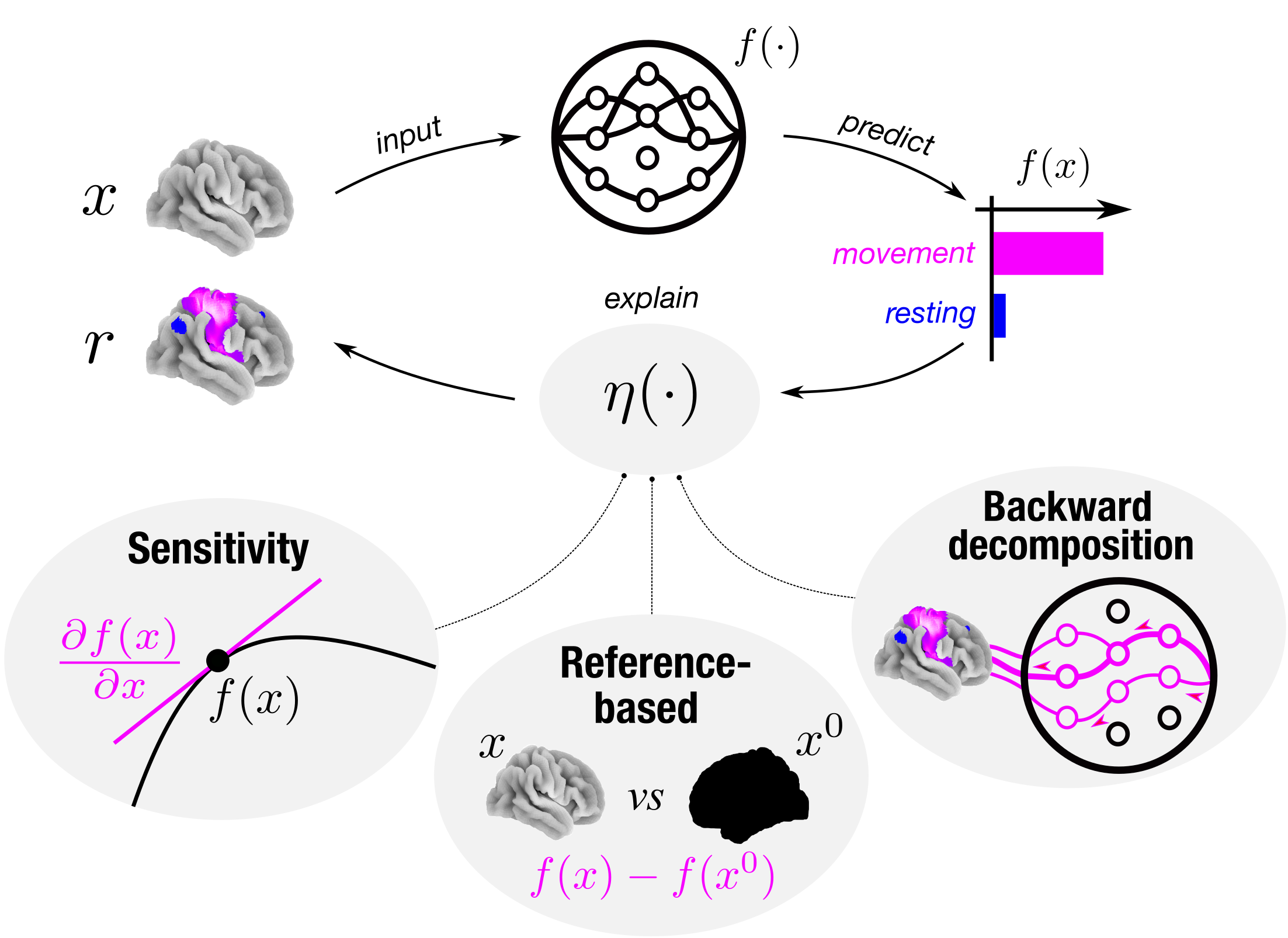
Figure 1: Attribution approaches. All considered attribution approaches $\eta(\cdot)$ seek to explain a mental state decoding decision $f(x)$ of model $f(\cdot)$ by attributing a relevance $r$ to each feature of the input $x$ for the decision. Backward decompositions attribute relevance to input features by decomposing the decoding decision in a backward pass through the model into the contributions of lower-level model units to the decision, up to the input space, where a contribution for each input feature can be defined. Reference-based attributions, by contrast, attribute relevance to input features by comparing the model’s response to a given input to its response to a reference input $x^{0}$, often chosen to be neutral. Sensitivity analyses, on the other hand, attribute relevance to input features according to how sensitively a model’s decoding decision responds to an input feature’s value.

We assume that the analyzed model represents some function $f(\cdot)$ mapping an input $x\in\mathbb{R}^{N}$ to some output $f(x)\in\mathbb{R}$, such that: $f(\cdot):\mathbb{R}^{N}\xrightarrow{}\mathbb{R}$. In the following, we present a set of attribution methods $\eta(\cdot)$ that seek to provide insights into this mapping by attributing a relevance score $r_{n}$ to each input feature $n=1,...,N$, quantifying its contribution to $f(x)$, such that: $\eta(\cdot):\mathbb{R}\xrightarrow{}\mathbb{R}^{N}$.

On a high level, the presented attribution methods can be divided into sensitivity analyses, reference-based attribution methods, and backward decompositions (see Fig. 1). Sensitivity analyses quantify $r$ by determining how sensitively $f(x)$ responds to $x$. Reference-based attributions, by contrast, determine $r$ by contrasting the model’s response to a given input $x$ to its response to a reference input $b$. Backward decompositions, on the other hand, quantify $r$ by sequentially decomposing the model’s output $f(x)$ in a backward pass through the model into the contributions of the lower-layer model units to the predictions, until the input space is reached and a contribution for each input feature can be defined.

Gradient Analysis (Zurada et al., , 1994, Simonyan et al., , 2014):

represents the most commonly used type of sensitivity analysis and defines $r_{n}$ as the partial derivative of $f(x)$ with respect to the input $x_{n}$, such that: $r_{n}=|\frac{\partial f(x)}{\partial x_{n}}|$. Relevance is thus assigned to those feature values to which $f(x)$ responds most sensitively.

SmoothGrad  (Smilkov et al., , 2017):

represents an extension of Gradient Analysis to account for sharp fluctuations of the gradient $\nabla f(x)=\frac{\partial f(x)}{\partial x}$ at small scales, which can otherwise lead to noise in the resulting attributions. SmoothGrad therefore first randomly draws $K$ samples (we set $K=50$) from the neighborhood of $x$ by adding random Gaussian noise $\mathcal{N}(0,\sigma^{2})$ with standard deviation $\sigma$ (we set $\sigma=1$) to $x$, and subsequently averages the resulting absolute partial derivatives for each random sample to obtain relevances $r$: $r=\frac{1}{K}\sum_{1}^{K}|\nabla f(x+\mathcal{N}(0,\sigma^{2}))|$.

InputXGradient (Shrikumar et al., , 2017):

represents another extension of Gradient Analysis, which multiplies the gradient $\nabla f(x)$ by $x$, such that: $r=\nabla f(x)\times x$ (where $\times$ indicates the element-wise product). The intuition behind this approach comes from linear models, where the product of input and model coefficient (here represented by the gradient) corresponds to the total contribution of the associated feature to the model’s output.

Guided Backpropagation (Springenberg et al., , 2015):

represents an adaptation of Gradient Analysis tailored to CNN models that primarily use ReLU Agarap, (2019) activation functions. It overrides gradients of ReLU activation functions in the computation of the gradient $\nabla f(x)$ such that only non-negative gradients are backpropagated.

Guided Gradient-weighted Class Activation Mapping (Guided GradCam) (Selvaraju et al., , 2017):

represents another type of sensitivity analysis tailored to CNNs that combines Guided Backpropagation with the GradCam (Selvaraju et al., , 2017) technique. Specifically, GradCam first computes the gradient $\nabla f(x)$ with respect to the feature maps $A^{k}\in\mathbb{R}^{D}$ of the last convolutional layer $L$ closest to the model’s output ($\frac{\partial f(x)}{\partial A^{k}}$) and then global-average pools the resulting gradients to obtain an importance weight $\alpha_{k}$ for each kernel $k\in L$: $\alpha_{k}=\frac{1}{D}\sum_{d=1}^{D}\frac{\partial f(x)}{\partial A_{d}^{k}}$. Conceptually, $a_{k}$ captures the importance of feature map $A^{k}$ for the decoded mental state. Next, GradCam uses the importance weights $\alpha_{k}$ to combine the activation maps $A^{k}$ to an aggregate heatmap of relevances $r_{A}$: $r_{A}=\sigma(\sum_{k}\alpha_{k}A^{k})$, where $\sigma$ represents the ReLU function ($\sigma(x)=max(0,x)$). Last, to obtain relevances $r$, Guided GradCam upsamples the relevances $r_{A}$ to the original input dimension and multiplies the upsampled maps with the relevance attributions of an application of Guided Backpropagation to $f(x)$ (see above).

Integrated Gradients (Sundararajan et al., , 2017):

represents a reference-based attribution method that assigns relevance $r$ by integrating the gradient $\nabla f(x)$ along a linear trajectory in the input space, connecting the current input $x$ to some neutral reference input $b$: $r^{b}=(x-b)\int_{\alpha=0}^{1}\frac{\delta f(b+\alpha(x-b))}{\delta x}$. Integrated Gradients thus assigns relevance to input features according to how much the model’s output changes when these features are scaled from the reference value to their current value. In our analyses, we chose two reference inputs, namely, an all-zero input $b^{0}$ (as recommended in Sundararajan et al., , 2017) as well as an average over all inputs in the analyzed dataset $b^{\mu}$, and averaged over the two resulting attributions to obtain relevance values $r$: $r=0.5r^{0}+0.5r^{\mu}$.

Deep Learning Important FeaTures (DeepLift) DeepLift (Shrikumar et al., , 2017):

represents another type of reference-based attribution method. Similar to Integrated Gradients, DeepLift determines relevances $r$ by comparing model responses for a given input $x$ to the model’s response to some neutral reference input $b$. To this end, DeepLift defines a contribution score $C_{\Delta x_{n}\Delta f(x)}$, describing the difference-from-reference response $\Delta f(x)=f(x)-f(b)$ that is attributed to a difference-from-reference in the input $\Delta x=x-b$. Note that $\sum_{n=1}^{N}C_{\Delta x_{n}\Delta f(x)}=\Delta f(x)$. To compute these contribution scores, DeepLift uses multipliers $m_{\Delta x_{n}\Delta f(x)}$ that are defined as $m_{\Delta x\Delta f(x)}=\frac{C_{\Delta x\Delta f(x)}}{\Delta x}$ and thereby quantify the contribution of $\Delta x$ to $\Delta f(x)$, scaled by $\Delta x$. For any unit $x^{(l)}$ in model layer $l$ and any unit $x^{(l-1)}$ in the preceding layer $l-1$, these multipliers can be computed as: $m_{\Delta x^{(l-1)}_{n}\Delta f(x)}=\sum_{j}m_{\Delta x^{(l-1)}_{n}\Delta x^{(l)}_{j}}m_{\Delta x^{(l)}_{j}\Delta f(x)}$ (where $\Delta x^{(l)}_{j}$ indicates the difference in input feature $j$ of layer $l$ to its value for the reference input), in line with the chain rule. Relevance $r_{n}$ for input feature $n$ can then be obtained as: $r_{n}=C_{\Delta x_{n}\Delta f(x)}=\Delta x_{n}m_{\Delta x_{n}\Delta f(x)}$. In its basic formulation, DeepLift uses two rules to compute contribution scores: The linear rule applies to dense and convolution layers, which compute $a=w^{0}+\sum_{n}w_{n}x_{n}$ (where $w^{0}$ and $w$ indicate bias and weights and $x$ the input), and defines $C_{\Delta x_{n}\Delta a}=\Delta x_{n}w_{n}$ and accordingly $m_{\Delta x_{n}\Delta a}=\frac{C_{\Delta x_{n}\Delta a}}{\Delta x_{n}}$. The rescale rule applies to all non-linear transformations $\sigma(a)$ (e.g., ReLU or sigmoid functions) and defines $C_{\Delta x\Delta\sigma(a)}=\Delta\sigma(a)$ and accordingly $m_{\Delta x\Delta\sigma(a)}=\frac{C_{\Delta x\Delta\sigma(a)}}{\Delta x}$.

DeepLift SHapley Additive exPlanation (DeepLift SHAP) (Lundberg and Lee, , 2017):

combines DeepLift with SHAP, a method for computing Shapley values (Shapley, , 1952) for a conditional expectation function of the analyzed model. Specifically, SHAP values attribute to each input feature the change in expected model prediction conditioned on a feature of interest. To approximate SHAP values using DeepLift for a given input $x$, DeepLift SHAP draws $K$ (we set $K=50$) random samples from the data (to approximate the set of other possible feature coalitions) and averages over the DeepLift attributions for each random sample, when treating the random sample as a reference input $b$.

Layer-wise relevance propagation (LRP) (Bach et al., , 2015):

represents a backward decomposition method. Let $i$ and $j$ be the indices of two models units in successive model layers $l$ and $l+1$ and $r_{j}^{(l+1)}$ the relevance of unit $j$ for $f(x)$. To redistribute relevance between layers, several rules have been proposed (Bach et al., , 2015, Montavon et al., , 2019, Kohlbrenner et al., , 2020), which generally follow from $r_{i}^{(l)}=\sum_{j}\frac{a_{i}w_{ij}}{\sum_{i}a_{i}w_{ij}}r_{j}^{(l+1)}$ (where $a$ and $w$ represent the input and weight of model unit $i$ in layer $l$). Importantly, LRP conserves relevance between layers, such that: $\sum_{n}r_{n}=\sum_{i}r_{i}^{(l)}=\sum_{j}r_{j}^{(l+1)}=f(x)$. In line with the recommendations by (Montavon et al., , 2019), we use a composite of relevance redistribution rules, namely, the LRP-0 rule ($r_{i}^{(l)}=\sum_{j}\frac{a_{i}w_{ij}}{\sum_{i}a_{i}w_{ij}}r_{j}^{(l+1)}$) for the dense output layer and the LRP-$\gamma$ rule ($r_{i}^{(l)}=\sum_{j}\frac{a_{i}(w_{ij}+\gamma w_{ij}^{+})}{\sum_{i}a_{i}(w_{ij}+\gamma w_{ij}^{+})}r_{j}^{(l+1)}$, where $\gamma$ controls the positive contributions to $r$ (we set $\gamma=0.25$)) for all convolution layers.

1.6 Statistical modelling

For the statistical comparison of attribution methods on any metric, we estimate linear regression models that include one binary indicator variable for all attribution methods other than DeepLift, which we treat as unmodelled baseline. We fit all regression models in a Bayesian framework by the use of the Bayesian Model-Building Interface (bambi 0.9.0; Capretto et al., , 2022) and by sampling four chains per parameter ($5,000$ samples per chain after $5,000$ discarded tuning samples) using the Markov chain Monte Carlo No-U-Turn-Sampler (NUTS; Hoffman and Gelman, , 2014) with bambi’s automatically generated priors. We determine a method as meaningfully different from DeepLift on the analyzed metric if the estimated $94\%$ highest-density interval of the method’s coefficient does not include $0$. All posterior traces are checked for convergence according to the Gelman–Rubin statistic ($|\hat{R}-1|<.01$).

1.7 Code and data availability

All custom code that we use for the analyses of this study as well as the trial-level BOLD maps are available at: github.com/athms/interpreting-brain-decoding-models.

2 Results

The target of our decoding analyses was to correctly decode the mental state associated with each trial-level BOLD map (namely, ”heat” and ”rejection” for the heat-rejection dataset, ”left foot (lf)”, ”right foot (rf)”, ”left hand (lh)”, ”right hand (rh)”, and ”tongue (t)” for the MOTOR dataset, and ”body”, ”faces”, ”places”, and ”tools” for the WM dataset; see section 1.1.1).

2.1 Hyper-parameter optimization

To determine a set of model and optimization hyper-parameters for each dataset, we performed a grid search over 144 unique parameter sets (see section 1.4.2) and evaluated the performance of each of these configurations in a three-fold cross-validation procedure, using each dataset’s training data (see section 1.3). We then determined the best-performing configuration by computing each configuration’s mean decoding error $\epsilon$ (defined as $1$ minus the fraction of correctly decoded trial-level BOLD maps) in the training and validation datasets over the three folds ($\epsilon^{T}$ and $\epsilon^{V}$ respectively) and assigning a performance score $\lambda_{i}$ to each configuration $i$: $\lambda_{i}=\epsilon^{V}_{i}+|\epsilon^{V}_{i}-\epsilon^{T}_{i}|$. This score quantifies how well a model performed in the validation data when also accounting for the difference in model performance to the training data. Accordingly, we defined the best performing configuration for each dataset as the one with the lowest $\lambda_{i}$ (see Table 1).

Table 1: Best-performing model and optimization configurations. For each dataset, the number of 3D-convolution layers, number of kernels per convolution layer, size of the kernels, training mini-batch size (BS), learning rate (LR), and dropout rate are shown for the configuration with lowest $\lambda_{i}$ (indicating best performance; see section 2.1)

Dataset # Layers # Kernels Kernel size BS LR Dropout heat-rejection 4 8 3 32 0.001 0.5 MOTOR 3 8 3 32 0.001 0.5 WM 4 16 5 64 0.001 0.5

2.2 Models accurately decode mental states

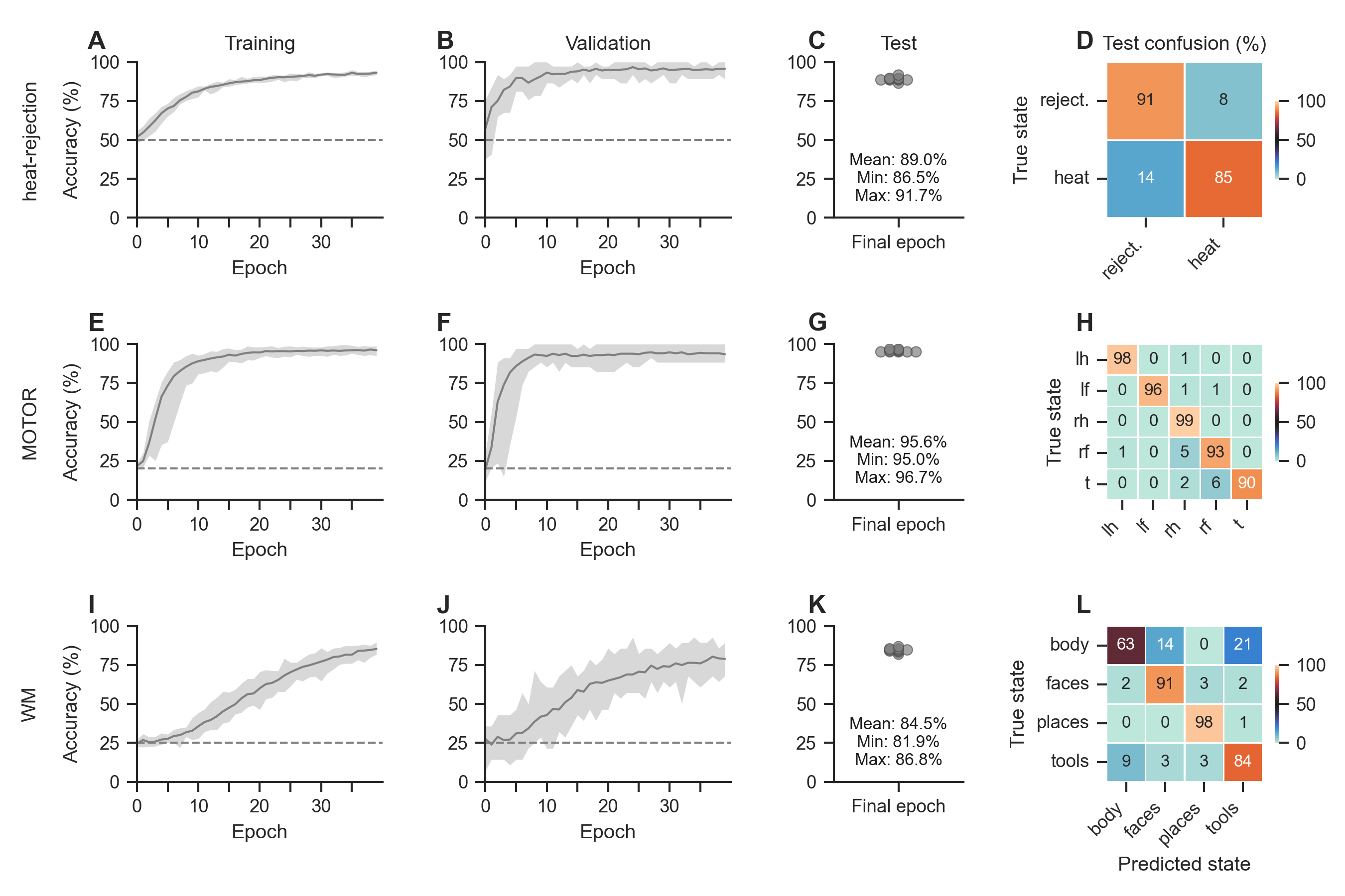
Figure 2: Decoding performance. For each dataset, we trained ten identical variants of each datasets’ model and optimization configuration (see section 2.2 of the main text for details on hyper-parameter selection) and solely varied the random seed between training runs and the random split of the data into training and validation datasets (95% and 5% of the full training data respectivelyy). A-B,E-F,I-J: The configurations performed well in decoding the mental states from the trial-level maps in the training (A,E,I) and validation datasets (B,F,J). Lines indicate mean decoding accuracies with shaded areas indicating respective minimum and maximum decoding accuracies across the ten training runs. Dashed line indicates chance accuracy. C-D,G-H,K-L: The final models also performed well in decoding the mental states of the left-out test datasets (C,G,K) with overall low average confusion rates (D,H,L). Scatter points indicate the final decoding accuracies in the test data.

Several recent findings in DL research have demonstrated that DL model performances are strongly dependent on many non-deterministic aspects of their training, such as, random weight initializations and random shufflings of the data during training (Thomas et al., 2021b, , Lucic et al., , 2018, Henderson et al., , 2018). To this end, we performed ten training runs with the best-performing model and optimization configuration of each dataset (see section 2.1), with different random seeds and training/validation data splits per run. For each run, we divided the dataset’s training data (see section 1.3) into new training and validation datasets by randomly selecting $5\%$ of the trial-level BOLD maps as validation data and using the remaining maps for training. We then trained models for $40$ epochs on the training data (Fig. 2 A-B,E-F,I-J) before evaluating the model’s decoding performance in the left-out test dataset (containing the data of every 5th subject of the full dataset; see Fig. 2 C-D,G-H,K-L).

The models performed well in decoding the mental states of each dataset, with average test decoding accuracies of 89.0% [86.5%, 91.7%] (heat-rejection), 95.6% [95%, 96.7%] (MOTOR), and 84.5% [81.9%, 86.8%] (WM) (reported as mean [min, max]) (Fig. 2 C,G,K). We also computed average test confusion rates over the ten training runs and found that the models exhibited little confusion between the mental states (Fig. 2 D,H,L)).

2.3 Explanations of sensitivity analyses are biologically more plausible

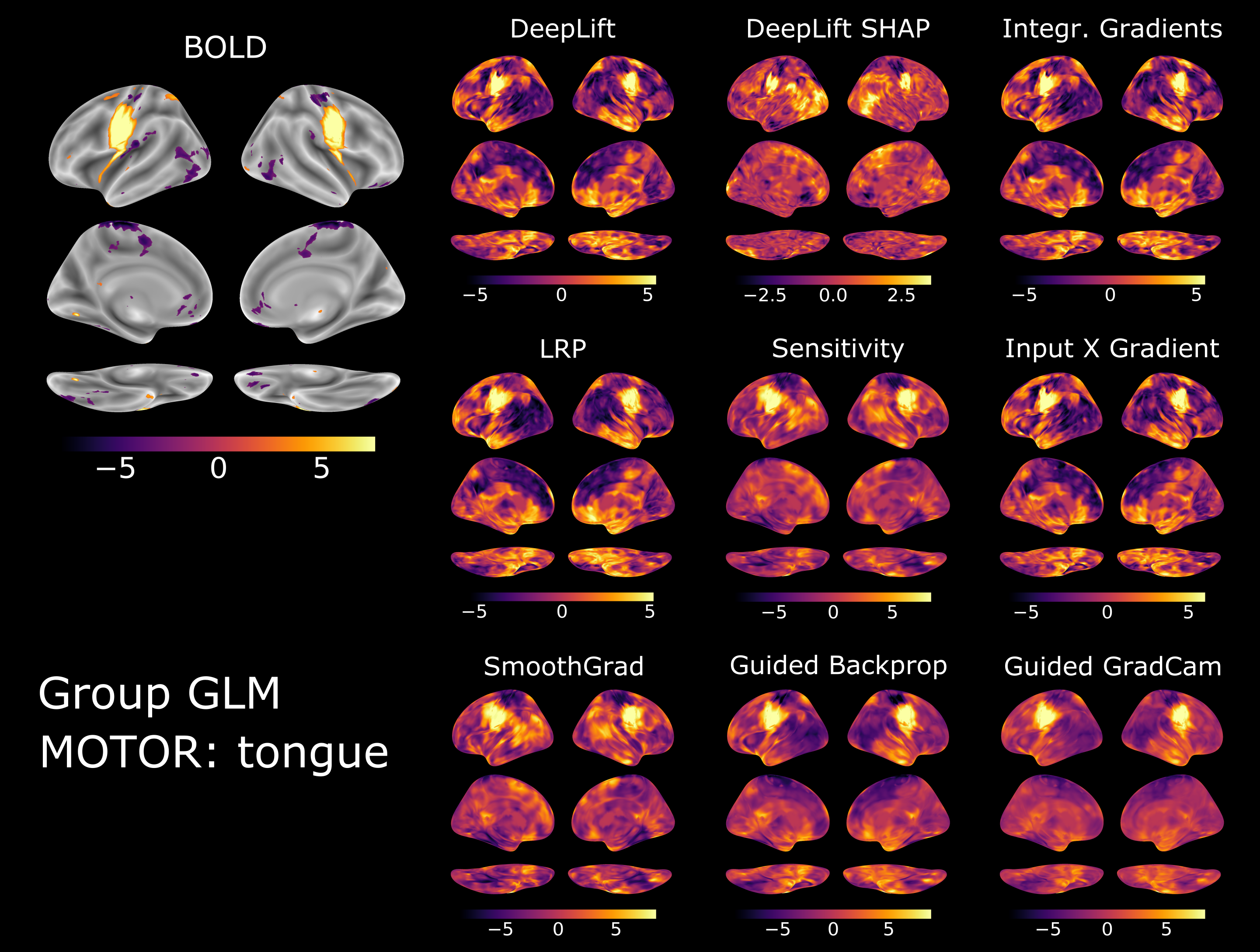
Figure 3: Group-level brain maps for ”tongue” movements of the MOTOR dataset. For each dataset, we performed a two-stage random effects GLM analysis of the trial-level BOLD maps as well as the attributions of each attribution method for test trial-level BOLD maps. Brain maps show the resulting Z-scores of a contrast between the ”tongue” state and all other mental states of the MOTOR dataset. All brain maps are projected onto the inflated cortical surface of the FsAverage template (Fischl, , 2012). We thresholded the group-level BOLD contrast map at a false positive rate of $0.01$.

As the trained models performed well in decoding the mental states of the three datasets (see Fig. 2), we proceeded to compare the attribution methods’ effectiveness in providing insight into the models’ learned mappings between brain activity and mental states. To this end, we interpreted the decoding decisions of each of the ten trained model instances per dataset (see section 2.2) with each attribution method (see section 1.5) for the trial-level BOLD maps of the corresponding test dataset (see section 1.3). Importantly, we always interpreted the models’ decoding decision for the actual mental state associated with each trial-level BOLD map. This analysis resulted in a dataset of ten attribution maps (one per model instance) for each attribution method and trial-level BOLD map.

To aggregate these attribution data over the ten model training runs, we performed a standard two-stage GLM analysis by first computing a subject-level GLM analysis of the trial-level attribution maps and subsequently aggregating the subject-level attribution maps in a random-effects group-level analysis (for details on the GLM analysis, see section 1.2.2). Importantly, the subject-level analysis included additional binary nuissance variables for the ten model training runs as well as the sum of the attribution values of each trial-level attribution map (as attribution sums can vary between decoding decisions, e.g., due to varying model decoding certainty).

To also identify the set of voxels whose activity we would expect to be associated with each mental state in a standard analysis of the BOLD data, we repeated this GLM analysis procedure for the trial-level BOLD maps of each dataset (without the additional nuisance regressors).

Figure 3 provides an overview of the resulting group-level BOLD and attribution maps for the ”tongue” movement state of the MOTOR dataset. For this state, the attribution methods correctly attributed high relevance to those voxels in the ventral premotor and primary motor cortex that also showed high activity in the group-level analysis of the BOLD data.

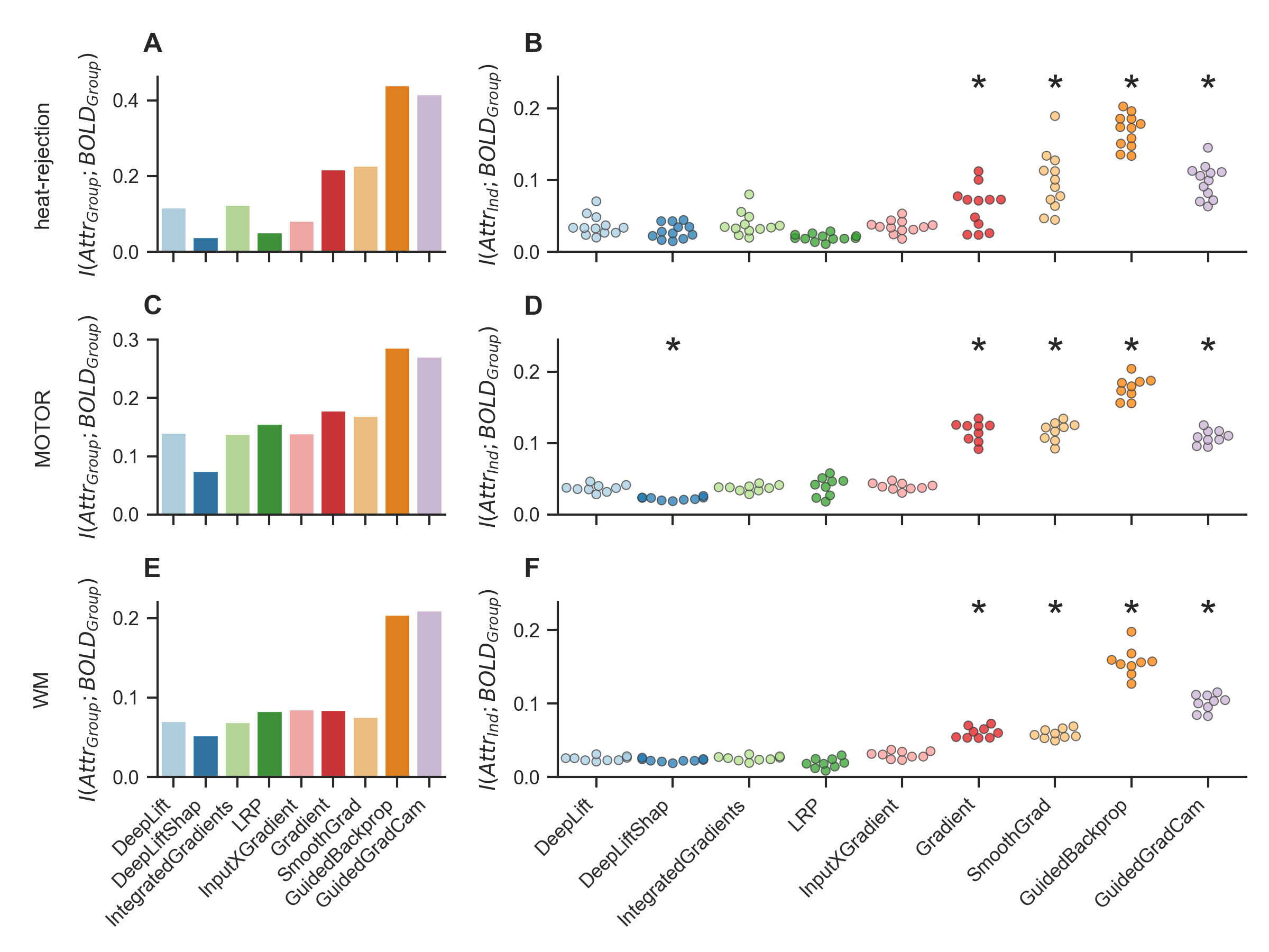
Figure 4: Similarity of attribution maps to group-level BOLD maps. To estimate similarity, we compute the mutual information between the group-level BOLD maps and the group- (A,C,E) and subject-level (B,D,F) attribution maps for each mental state. A,C,E: The group-level maps of Guided Backpropagation and Guided GradCam exhibit overall higher mutual information (i.e., similarity) with the group-level BOLD maps than the group-level maps of the other attribution methods. Bar heights indicate mean mutual information over the mental states of a dataset. B,D,F: Similarly, the subject-level maps of Guided Backpropagation, Guided GradCam as well as Gradient Analysis and SmoothGrad exhibit higher mutual information with the group-level BOLD maps than the subject-level maps of the other attribution methods. Scatter points indicate mean mutual information per subject. Black stars indicate that the distribution of subject means is meaningfully different from the distribution of the DeepLift method (for analysis details, see section 1.6). Colors indicate interpretation methods.

As can be seen, it is generally difficult to discern the quality of the various attributions by visual inspection alone. For this reason, we next took a quantitative approach to analyzing how well the attributions align with the results of the GLM analysis of the BOLD data by computing the average mutual information (Kraskov et al., , 2004) between the group-level attribution maps and the corresponding group-level BOLD maps for the same mental state (see Fig. 4 A,C,E). Note that we chose mutual information as a similarity measure because the association between the group-level BOLD and attribution maps does not need to be linear. For example, it is possible that a DL model learns to identify a mental state through the activity of voxels that are meaningfully more active in this state as well as the activity of voxels that are meaningfully less active, resulting in an attribution map that assigns high relevance to voxels that exhibit high positive and negative values in a GLM analysis of the BOLD data (Thomas et al., 2021a, ).

This analysis revealed that the group-level attribution maps of Guided Backpropagation (Springenberg et al., , 2015) and Guided GradCam (Selvaraju et al., , 2017), two types of sensitivity analysis (see section 1.5), are more similar to the group-level BOLD maps than those of the other attribution methods (as indicated by average higher mutual information scores), while the group-level maps of Gradient Analysis (Simonyan et al., , 2014) and SmoothGrad (Smilkov et al., , 2017), again two types of sensitivity analyses, exhibit less, but still comparably high similarity, to the group-level BOLD maps when compared to the remaining attribution methods (Fig. 4 A,C,E).

We also tested how well the subject-level attribution maps of each attribution method align with the group-level BOLD maps, as the trained models can draw from their knowledge about the group of subjects in their training data when decoding the trial-level BOLD maps of the test datasets. To this end, we computed the mutual information between the subject-level attribution maps and the corresponding group-level BOLD map of the same mental state and regressed the average mutual information per subject onto a set of binary dummy variables indicating the attribution methods (for details on the regression analysis, see section 1.6). This analysis showed that the subject-level attribution maps of Guided Backpropagation, Guided GradCam, SmoothGrad, and Gradient Analysis, all variants of sensitivity analysis, are generally more similar to the group-level BOLD maps than the subject-level attribution maps of the other attribution methods (Fig. 4 B,D,F).

2.4 Explanations of reference-based attributions and backward decompositions are more faithful

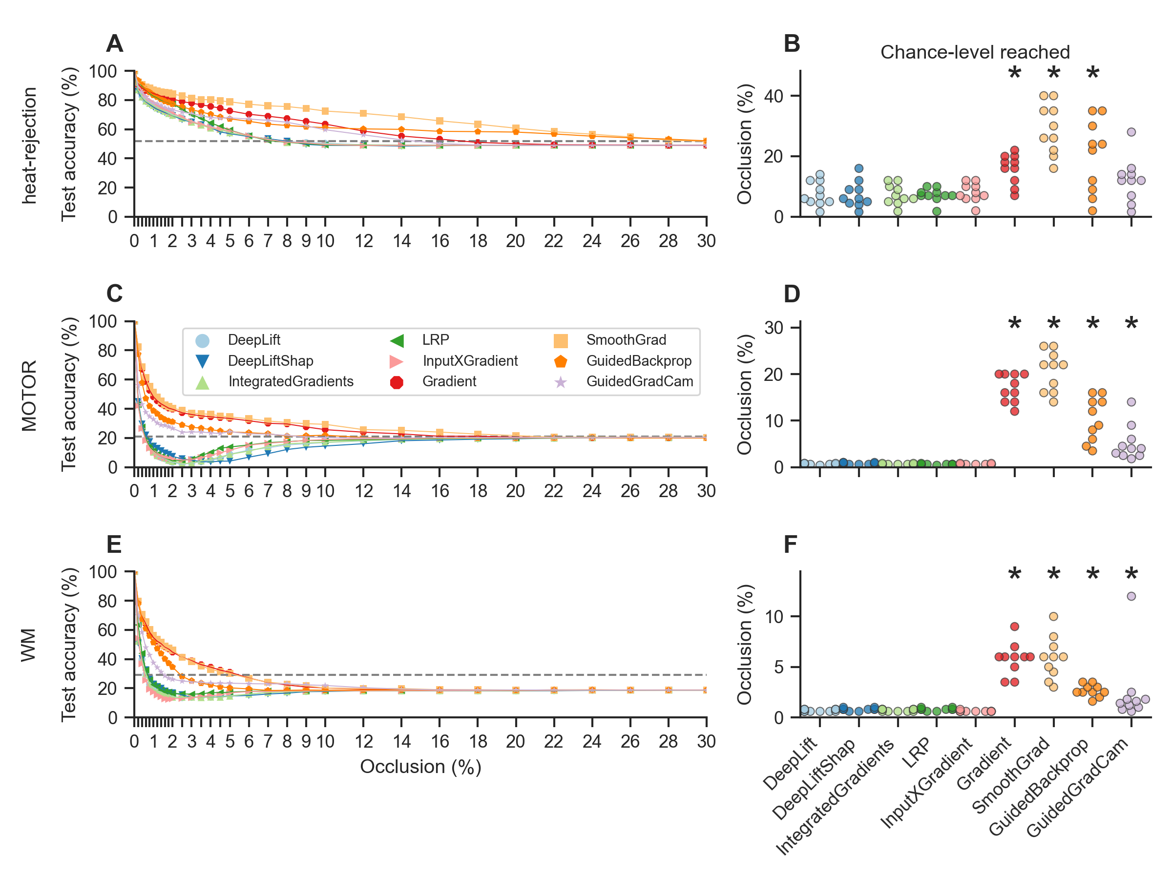
Figure 5: Attribution faithfulness. We estimated explanation faithfulness of an attribution method by repeatedly evaluating the models’ test decoding accuracy when occluding different fractions of the input voxels based on the relevance assigned to them by the attribution method, such that $0\%$ occlusion indicates that no voxel values were occluded while $50\%$ indicates that the values of all input voxels were occluded that received the highest $30\%$ of relevance values. For each attribution method and trained model, we recorded the occlusion rate at which the models’ test decoding accuracy first dropped to chance-level, indicating that all information has been removed from the data that the model uses to correctly identify the mental states. A,C,E: DeepLift, DeepLift SHAP, Integrated Gradients, LRP, and InputXGradient exhibit higher attribution faithfulness than Gradient Analysis, SmoothGrad, Guided Backpropagation, and Guided GradCam, as the models’ test decoding accuracies decrease more rapidly with increasing occlusion rates for these methods. Lines indicate mean test decoding accuracies over the ten training runs of each model and optimization configuration. B,D,F: Accordingly, model test decoding accuracies also drop to chance-level at lower occlusion rates for these approaches. Scatter points represent model training runs and black stars indicate that the distribution of occlusion rates is meaningfully different from the distribution of the DeepLift method (for analysis details, see section 1.6). Colors indicate interpretation methods.

In addition to understanding how the explanations of each attribution method compare to the results of a standard GLM analysis of the BOLD data, we were interested in understanding how well they perform at capturing the decision process of the trained models. To this end, we analyzed their explanation faithfulness (Samek et al., , 2021, 2017). An explanation can generally be considered as being faithful if it correctly identifies those features of the input that are most relevant for the model’s decoding decision. Accordingly, we tested whether removing those voxels from the input that received high relevance by an attribution method (by setting their values to 0) affects the model’s ability to correctly identify the mental states. To quantify faithfulness, we repeated this analysis for different occlusion rates, from $0\%$ (indicating no occlusion) to $50\%$ (indicating that those voxels are occluded that received the highest $50\%$ of relevance values) (Fig. 5 A,C,E) and recorded the occlusion rate at which the model’s decoding accuracies first dropped to chance level, indicating that all information has been removed from the data that the model requires to accurately identify the mental states (Fig. 5 B,D,F). If an attribution method has high explanation faithfulness, the model’s decoding accuracy should drop to chance level at lower occlusion rates when compared to methods with lower faithfulness.

Overall, this analysis revealed that reference-based attributions and backward decompositions, namely, DeepLift, DeepLift SHAP, Integrated Gradients, LRP generally exhibit higher explanation faithfulness than the tested sensitivity analyses because the models’ decoding decisions dropped to chance level at lower occlusion rates for these methods than for the others (with the exception of the InputXGradient (Shrikumar et al., , 2017) method whose explanations exhibited similar faithfulness to the tested backward decompositions and reference-based attributions; Fig. 5).

2.5 Sanity checks for attribution methods

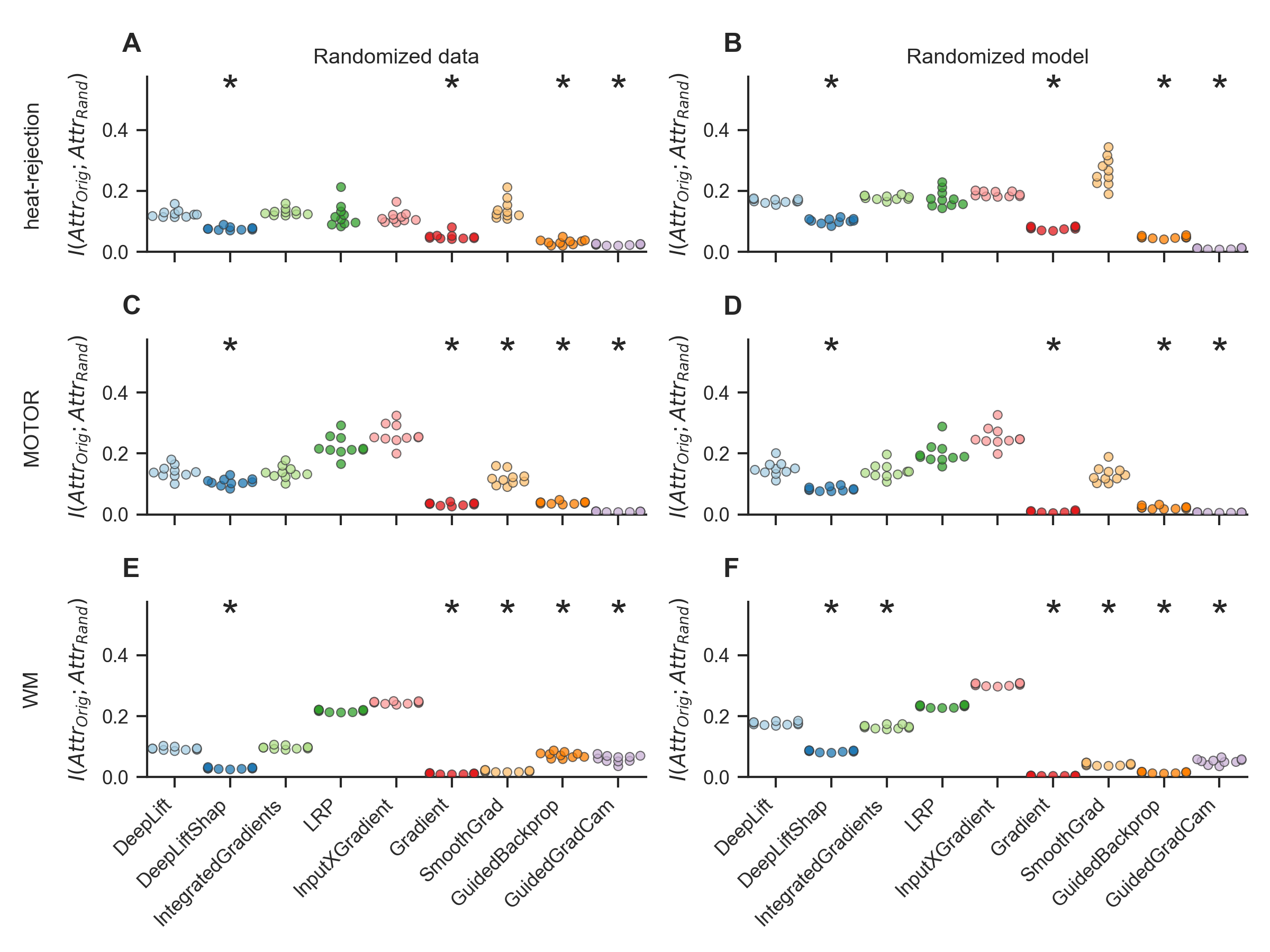
Figure 6: Sanity checks for attribution methods. We performed two sanity for each attribution method by comparing a method’s original attributions to its attributions for the same data when interpreting the mental state decoding decisions of a model variant trained on a version of the training data with randomized labels (data randomization test; A, C, E) and model with randomized weights (model randomization test; B, D, F). If the attributions of an attribution method are sensitive to the characteristics of the input data and model, its attributions for the original model should be different from its attributions for the model trained on randomized data as well as the model with random weights (leading to low mutual information scores). Overall, DeepLift SHAP, Gradient Analysis, Guided Backpropagation, and Guided GradCam performed better than the other methods in both tests (as indicated by generally lower mutual information scores), while DeepLift and Integrated Gradients also performed comparably well. Scatter points indicate mean mutual information for each model training run. Black stars indicate that the distribution of mean mutual information scores is meaningfully lower than the distribution of the DeepLift method (for analysis details, see section 1.6). Colors indicate interpretation methods.

Last, we performed two sanity checks for attribution methods, as recently proposed by Adebayo et al., (2018), to test the overall scope and quality of their explanations. Specifically, Adebayo et al., (2018) propose two simple tests to test whether the explanations of an attribution method are specific to the tested model and data by testing how much the explanations change when the method is applied to a model with the same architecture but random weights (the model randomization test) or a model trained on a version of the data with randomly permuted labels (the data randomization test). If the explanations are dependent on the specific parameters of the model, they should differ between the originally trained models and models with random weights. If the explanations are similar, however, the attribution method can be considered insensitive to the studied model and therefore not well-suited to capture the models’ decision process. Similarly, if the explanations of an attribution method account for the labeling of the data, it should produce explanations that are different between models model trained on the original dataset and models trained on a version of the data with randomly shuffled labels. If the explanations are similar, however, the attribution method can be considered independent of the labeling of the data and therefore not well-suited to understand the model’s learned mapping between these labels and the input data.

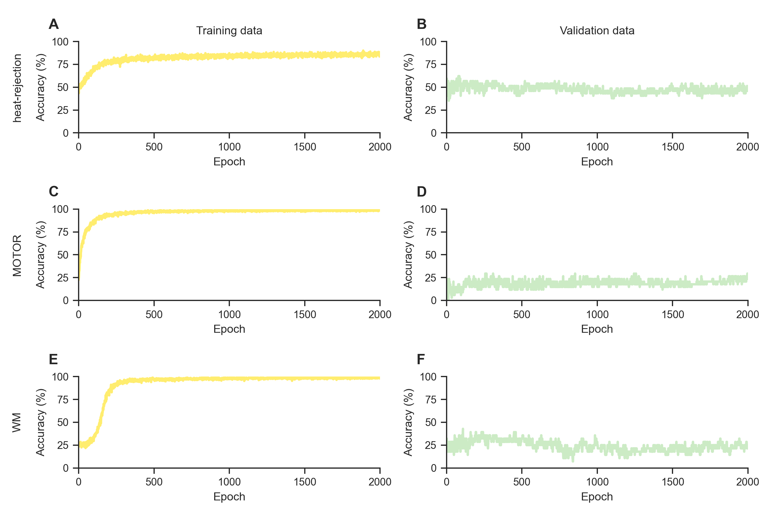
Figure A1: Model performances in the data randomization test. We trained one DL model, according to each dataset’s model configuration (see section 2.1 of the main text), on a variant of each dataset with permuted mental state labels. A,C,E: All models learn to decode the randomized mental state labels well in the training data. B,D,F: Yet, the models perform close to chance in decoding the randomized labels from the validation data, indicating that the models simply learned to memorize the mapping between trial-level BOLD maps and mental state labels of the training data. As in our other analyses (see section 2.2 of the main text), we randomly separated each dataset’s training data into new distinct training and validation datasets, comprising $95\%$ and $5\%$ of the data respectively. Colors indicate training (yellow) and validation (green) data. Lines indicate decoding accuracies over the course of training.

In line with the data randomization test, we first trained each model configuration on a version of its original training dataset with randomly shuffled mental state labels. The models were able to correctly decode the randomly shuffled mental state labels in their training data after $2,000$ training epochs, achieving decoding accuracies of $85.1\%$, $98.7\%$, and $98.4\%$ for the heat-rejection, MOTOR, and WM datasets respectively (Appendix Fig. A1). Importantly, the models’ validation decoding accuracies were still close to chance (namely, $45.9\%$, $23.5\%$, and $25\%$ for the heat-rejection, MOTOR, and WM datasets respectively; Appendix Fig. A1), indicating that the models memorized the random associations between labels and training data. When comparing the attributions of each attribution method for the test mental state decoding decisions of the models trained on the randomized and original training data, we found that the attributions of DeepLift SHAP, Gradient Analysis, SmoothGrad, Guided Backpropagation, and Guided GradCam were generally more dissimilar between the two models than those of the other attribution methods, indicating stronger dependence of their attributions on the characteristics of the data.

Similarly, in line with the model parameter randomization test, we also interpreted the test mental state decoding decisions of a randomly initialized variant of each datasets’ model configuration. As for the data randomization test, we compared the resulting attributions of each attribution method to the attributions for the originally trained models. Again, DeepLift SHAP, Gradient analysis, Guided Backpropagation, and Guided GradCam produced attributions that showed stronger dependence on the characteristics of the analyzed models, when compared to the other methods, as their attributions for the randomized and originally trained models were more dissimilar.

3 Discussion

With this work, we provide insights into the explanation performance of prominent types of attribution methods, namely, sensitivity analyses, backward decompositions, and reference-based attributions (see section 1.5), in mental state decoding analyses with DL models. To evaluate explanation performances, we use a diverse set of criteria: First, we evaluate the biological plausibility of the explanations by comparing them to the results of a standard GLM analysis of BOLD data, which seeks to identify all voxels whose activity pattern is associated with the mental states. We find that sensitivity analyses, such Guided Backpropagation, Guided GradCam, Gradient Analysis, and SmoothGrad, provide explanations that are more similar to the results of the GLM analysis, and thereby biologically more plausible, than the explanations of the tested backward decompositions and reference-based attributions. Second, we evaluate whether the explanations accurately capture the models’ decision process by testing whether they accurately identify all voxels of the input that the models rely on to identify the mental states. We find that backward decompositions and reference-based attributions, such as DeepLift, DeepLift SHAP, Integrated Gradients, and LRP, provide explanations that are more faithful than those of the tested sensitivity analyses. Last, to test whether the methods’ explanations are in fact sensitive to the analyzed model and data, we perform two sanity checks for attribution methods (as suggested by Adebayo et al., , 2018) and find that Gradient Analysis, Guided Backpropagation, Guided GradCam, DeepLift SHAP, DeepLift, and Integrated Gradients perform consistently well in both sanity checks, providing explanations that are sensitive to the characteristics of the analysed model and data.

3.1 Biological plausibility vs. explanation faithfulness

Our findings demonstrate a gradient between two key characteristics for the interpretation of mental state decoding decisions: attribution methods that provide highly faithful explanations, by capturing the model’s decision process well, also provide explanations that are biologically less plausible, because they do not necessarily identify all voxels whose activity patterns are associated with the mental states, when compared to interpretation methods with less explanation faithfulness. To make sense of this finding, it is important to remember that functional neuroimaging data generally exhibit strong spatial correlations, such that individual mental states are often associated with the activity of large clusters of voxels. DL models trained to identify these mental states from neuroimaging data will likely view some of this activity as redundant, as the activity of a subset of those voxels suffices to correctly identify the mental states. In these situations, any explanation of an attribution method with perfect faithfulness will not identify all voxels of the input whose activity is in fact associated with the decoded mental state, but solely the subset of voxels whose activity the model used as evidence for its decoding decision. Accordingly, attribution methods with high explanation faithfulness, such as backward decompositions and reference-based attributions, do not necessarily produce explanations that align well with the results of a standard GLM analysis of the BOLD data. By contrast, we found that sensitivity analyses, such as Guided GradCam, Guided Backpropagation, Gradient Analysis, and SmoothGrad, produce explanations that are less faithful but more in line with the results of a standard GLM analysis. Sensitivity analyses are less concerned with identifying the specific contribution of each input voxel to a decoding decision and instead focus on identifying how sensitively a model’s decision responds to (i.e., changes with) the activity of each voxel. With this perspective, sensitivity analyses identify a broader set of voxels whose activity the model takes into account when decoding the mental state, resulting in explanations that seem biologically more plausible because the set of identified voxels is more similar to that of standard analysis approaches for BOLD data, which seek to identify voxels whose activity pattern is associated with the mental state.

3.2 Recommendations for interpretation methods in mental state decoding

Based on these findings, we make a twofold recommendation for the application of attribution methods in mental state decoding:

If the goal of a mental state decoding analysis is to understand the decision process of the decoding model by identifying the parts of the input that are most relevant for the model’s decision, we generally recommend the application of backward decompositions or reference-based attributions. In particular, we recommend DeepLift, DeepLift SHAP, and Integrated Gradients because their explanations have shown overall high faithfulness in our analyses, while also performing well in the two sanity checks.

By contrast, if the goal of a mental state decoding analysis is to understand the association between the BOLD data and studied mental states, we recommend the application of sensitivity analyses, as these have shown to produce explanations with comparably high similarity to the results of a standard GLM analysis of the data when compared to reference-based attributions and backward decompositions. Particularly, for CNN models with ReLU activation functions, we recommend Guided Backpropagation and Guided GradCam as their explanations exhibit the overall highest similarity to the results of a standard GLM analysis of the BOLD data in our analyses, while also performing well in the two sanity checks. For models without ReLU activation functions, we recommend Gradient Analysis and SmoothGrad, as their explanations also have comparably high similarity to the results of the GLM analysis (especially on the level of individual subjects), while also performing well in the two sanity tchecks.

3.3 Caution in the interpretation of complex models

Last, we would like to advocate for caution in any interpretation of the mental state decoding decisions of DL models. DL models have an unmatched ability to learn from and represent complex data. Accordingly, their learned mappings between input data and decoding decisions can be highly complex and counterintuitive. For example, recent empirical work has shown that DL methods trained in mental state decoding analyses can identify individual mental states through voxels that exhibit meaningfully stronger activity in these states as well as voxels with meaningfully reduced activity in these states, leading to explanations that assign high relevance scores to voxels that receive both positive and negative weights in a standard GLM contrast analysis of the same BOLD data (Thomas et al., 2021a, ). To understand how a model’s weighting of the input in its decoding decision relates to the characteristics of the input data, it is therefore essential to compare the explanations of any attribution method to the results of standard analyses of the BOLD data (e.g., with linear models; Friston et al., , 1994, Kriegeskorte et al., , 2006, Grosenick et al., , 2013) as well as related empirical findings (e.g., as provided by NeuroSynth; Yarkoni et al., , 2011).

Similarly, a wealth of recent empirical work in machine learning research has demonstrated that DL models are prone to learning simple shortcuts (or confounds) from their training data, which do not generalize to other datasets (for a detailed discussion, see Geirhos et al., , 2020). A prominent example is a study that trained DL models to identify pneumonia from chest X-rays (Zech et al., , 2018). While the models performed well in the training data, comprising X-rays from few hospitals, their performance meaningfully decreased for X-rays from new hospitals. By applying attribution methods to the classification decisions of the trained models, the authors were able to show that the models learned to accurately identify the hospital system that was used to acquire an X-ray, in combination with the specific department, allowing them to make accurate predictions on aggregate by simply learning the overall prevalence rates of these departments. Similar examples are imaginable in functional neuroimaging, as recently suggested by Chyzhyk et al., (2022) who state that biomarker models for specific disease conditions could learn to distinguish patients from controls simply by their generally increased head motion.

For these reasons, we echo a recent call of machine learning researchers to always consider whether the application of complex models (such as DL models) is necessary to answer the research question at hand, or whether the application of simpler models, with better interpretability, could suffice (Rudin, , 2019). While we do believe that DL models hold a high promise for mental state decoding research, e.g., with their ability to learn from large-scale neuroimaging datasets (Schulz et al., , 2022), we also believe that many common mental state decoding analyses, which solely focus on few mental states in tens to a hundred of individuals, can be well-addressed with simpler decoding models with better interpretability (e.g., Hoyos-Idrobo et al., , 2018, Grosenick et al., , 2013, Kriegeskorte et al., , 2006, Michel et al., , 2011, Schulz et al., , 2020).

We hope that with this work we can provide some insights into the strengths and weaknesses of prominent interpretation methods in mental state decoding, thereby enabling neuroimaging researchers to make an informed choice in situations where explanations for the mental state decoding decisions of DL models are needed.

Acknowledgments.

We gratefully acknowledge the support of NIH under No. U54EB020405 (Mobilize), NSF under Nos. CCF1763315 (Beyond Sparsity), CCF1563078 (Volume to Velocity), and 1937301 (RTML); ARL under No. W911NF-21-2-0251 (Interactive Human-AI Teaming); ONR under No. N000141712266 (Unifying Weak Supervision); ONR N00014-20-1-2480: Understanding and Applying Non-Euclidean Geometry in Machine Learning; N000142012275 (NEPTUNE); NXP, Xilinx, LETI-CEA, Intel, IBM, Microsoft, NEC, Toshiba, TSMC, ARM, Hitachi, BASF, Accenture, Ericsson, Qualcomm, Analog Devices, Google Cloud, Salesforce, Total, the HAI-GCP Cloud Credits for Research program, the Stanford Data Science Initiative (SDSI), the Texas Advanced Computing Center (TACC) at The University of Texas at Austin, and members of the Stanford DAWN project: Facebook, Google, and VMWare. The U.S. Government is authorized to reproduce and distribute reprints for Governmental purposes notwithstanding any copyright notation thereon. Any opinions, findings, and conclusions or recommendations expressed in this material are those of the authors and do not necessarily reflect the views, policies, or endorsements, either expressed or implied, of NIH, ONR, or the U.S. Government.

FMRI data for the MOTOR and WM datasets were provided by the Human Connectome Project (HCP S1200 release), WU Minn Consortium (Principal Investigators: David Van Essen and Kamil Ugurbil; 1U54MH091657) funded by the 16 NIH Institutes and Centers that support the NIH Blueprint for Neuroscience Research; and by the McDonnell Center for Systems Neuroscience at Washington University. FMRI data for the heat-rejection dataset were publicly shared in a preprocessed format by Kohoutová et al., (2020).

Appendix A Methods

A.1 Data

A.1.1 Fmriprep details

Results included in this manuscript come from preprocessing performed using fMRIPrep 20.2.3 (Esteban et al., 2018b ; Esteban et al., 2018a ; RRID:SCR_016216), which is based on Nipype 1.6.1 (Gorgolewski et al., (2011); Gorgolewski et al., (2018); RRID:SCR_002502).

Anatomical data preprocessing

The T1-weighted (T1w) images were corrected for intensity non-uniformity (INU) with N4BiasFieldCorrection (Tustison et al., , 2010), distributed with ANTs 2.3.3 (Avants et al., , 2008, RRID:SCR_004757), and used as T1w-reference throughout the workflow. The T1w-reference was then skull-stripped with a Nipype implementation of the antsBrainExtraction.sh workflow (from ANTs), using OASIS30ANTs as target template. Brain tissue segmentation of cerebrospinal fluid (CSF), white-matter (WM) and gray-matter (GM) was performed on the brain-extracted T1w using fast (FSL 5.0.9, RRID:SCR_002823, Zhang et al., , 2001). Volume-based spatial normalization to two standard spaces (MNI152NLin2009cAsym, MNI152NLin6Asym) was performed through nonlinear registration with antsRegistration (ANTs 2.3.3), using brain-extracted versions of both T1w reference and the T1w template. The following templates were selected for spatial normalization: ICBM 152 Nonlinear Asymmetrical template version 2009c [Fonov et al., (2009), RRID:SCR_008796; TemplateFlow ID: MNI152NLin2009cAsym], FSL’s MNI ICBM 152 non-linear 6th Generation Asymmetric Average Brain Stereotaxic Registration Model [Evans et al., (2012), RRID:SCR_002823; TemplateFlow ID: MNI152NLin6Asym],

Functional data preprocessing

For each of the BOLD runs found per subject, the following preprocessing was performed. First, a reference volume and its skull-stripped version were generated using a custom methodology of fMRIPrep. Susceptibility distortion correction (SDC) was omitted. The BOLD reference was then co-registered to the T1w reference using flirt (FSL 5.0.9, Jenkinson and Smith, , 2001) with the boundary-based registration (Greve and Fischl, , 2009) cost-function. Co-registration was configured with nine degrees of freedom to account for distortions remaining in the BOLD reference. Head-motion parameters with respect to the BOLD reference (transformation matrices, and six corresponding rotation and translation parameters) are estimated before any spatiotemporal filtering using mcflirt (FSL 5.0.9, Jenkinson et al., , 2002). The BOLD time-series (including slice-timing correction when applied) were resampled onto their original, native space by applying the transforms to correct for head-motion. These resampled BOLD time-series will be referred to as preprocessed BOLD in original space, or just preprocessed BOLD. The BOLD time-series were resampled into standard space, generating a preprocessed BOLD run in MNI152NLin2009cAsym space. First, a reference volume and its skull-stripped version were generated using a custom methodology of fMRIPrep. Automatic removal of motion artifacts using independent component analysis (ICA-AROMA, Pruim et al., , 2015) was performed on the preprocessed BOLD on MNI space time-series after removal of non-steady state volumes and spatial smoothing with an isotropic, Gaussian kernel of 6mm FWHM (full-width half-maximum). Corresponding “non-aggresively” denoised runs were produced after such smoothing. Additionally, the “aggressive” noise-regressors were collected and placed in the corresponding confounds file. Several confounding time-series were calculated based on the preprocessed BOLD: framewise displacement (FD), DVARS and three region-wise global signals. FD was computed using two formulations following Power (absolute sum of relative motions, Power et al., (2014)) and Jenkinson (relative root mean square displacement between affines, Jenkinson et al., (2002)). FD and DVARS are calculated for each functional run, both using their implementations in Nipype (following the definitions by Power et al., , 2014). The three global signals are extracted within the CSF, the WM, and the whole-brain masks. Additionally, a set of physiological regressors were extracted to allow for component-based noise correction (CompCor, Behzadi et al., , 2007). Principal components are estimated after high-pass filtering the preprocessed BOLD time-series (using a discrete cosine filter with 128s cut-off) for the two CompCor variants: temporal (tCompCor) and anatomical (aCompCor). tCompCor components are then calculated from the top 2% variable voxels within the brain mask. For aCompCor, three probabilistic masks (CSF, WM and combined CSF+WM) are generated in anatomical space. The implementation differs from that of Behzadi et al. in that instead of eroding the masks by 2 pixels on BOLD space, the aCompCor masks are subtracted a mask of pixels that likely contain a volume fraction of GM. This mask is obtained by thresholding the corresponding partial volume map at 0.05, and it ensures components are not extracted from voxels containing a minimal fraction of GM. Finally, these masks are resampled into BOLD space and binarized by thresholding at 0.99 (as in the original implementation). Components are also calculated separately within the WM and CSF masks. For each CompCor decomposition, the k components with the largest singular values are retained, such that the retained components’ time series are sufficient to explain 50 percent of variance across the nuisance mask (CSF, WM, combined, or temporal). The remaining components are dropped from consideration. The head-motion estimates calculated in the correction step were also placed within the corresponding confounds file. The confound time series derived from head motion estimates and global signals were expanded with the inclusion of temporal derivatives and quadratic terms for each (Satterthwaite et al., , 2013). Frames that exceeded a threshold of 0.5 mm FD or 1.5 standardised DVARS were annotated as motion outliers. All resamplings can be performed with a single interpolation step by composing all the pertinent transformations (i.e. head-motion transform matrices, susceptibility distortion correction when available, and co-registrations to anatomical and output spaces). Gridded (volumetric) resamplings were performed using antsApplyTransforms (ANTs), configured with Lanczos interpolation to minimize the smoothing effects of other kernels (Lanczos, , 1964). Non-gridded (surface) resamplings were performed using mri_vol2surf (FreeSurfer).

Many internal operations of fMRIPrep use Nilearn 0.6.2 (Abraham et al., 2014b, ,
RRID:SCR_001362), mostly within the functional processing workflow. For more details of the pipeline, see the section corresponding to workflows in fMRIPrep’s documentation.

Copyright Waiver

The above boilerplate text was automatically generated by fMRIPrep with the express intention that users should copy and paste this text into their manuscripts unchanged. It is released under the CC0 license.

Appendix B Results

B.1 Data randomization test

References

- (1) Abraham, A., Pedregosa, F., Eickenberg, M., Gervais, P., Mueller, A., Kossaifi, J., Gramfort, A., Thirion, B., and Varoquaux, G. (2014a). Machine learning for neuroimaging with scikit-learn. Frontiers in Neuroinformatics, 8.
- (2) Abraham, A., Pedregosa, F., Eickenberg, M., Gervais, P., Mueller, A., Kossaifi, J., Gramfort, A., Thirion, B., and Varoquaux, G. (2014b). Machine learning for neuroimaging with scikit-learn. Frontiers in Neuroinformatics, 8.
- Adebayo et al., (2018) Adebayo, J., Gilmer, J., Muelly, M., Goodfellow, I., Hardt, M., and Kim, B. (2018). Sanity checks for saliency maps. In Proceedings of the 32nd International Conference on Neural Information Processing Systems, NIPS’18, pages 9525–9536, Red Hook, NY, USA. Curran Associates Inc.
- Agarap, (2019) Agarap, A. F. (2019). Deep Learning using Rectified Linear Units (ReLU). arXiv:1803.08375 [cs, stat]. arXiv: 1803.08375.
- Avants et al., (2008) Avants, B., Epstein, C., Grossman, M., and Gee, J. (2008). Symmetric diffeomorphic image registration with cross-correlation: Evaluating automated labeling of elderly and neurodegenerative brain. Medical Image Analysis, 12(1):26–41.
- Bach et al., (2015) Bach, S., Binder, A., Montavon, G., Klauschen, F., Müller, K.-R., and Samek, W. (2015). On Pixel-Wise Explanations for Non-Linear Classifier Decisions by Layer-Wise Relevance Propagation. PLOS ONE, 10(7):e0130140.
- Behzadi et al., (2007) Behzadi, Y., Restom, K., Liau, J., and Liu, T. T. (2007). A component based noise correction method (CompCor) for BOLD and perfusion based fmri. NeuroImage, 37(1):90–101.
- Capretto et al., (2022) Capretto, T., Piho, C., Kumar, R., Westfall, J., Yarkoni, T., and Martin, O. A. (2022). Bambi: A Simple Interface for Fitting Bayesian Linear Models in Python. Journal of Statistical Software, 103:1–29.
- Chyzhyk et al., (2022) Chyzhyk, D., Varoquaux, G., Milham, M., and Thirion, B. (2022). How to remove or control confounds in predictive models, with applications to brain biomarkers. GigaScience, 11:giac014.
- Ding and Koehn, (2021) Ding, S. and Koehn, P. (2021). Evaluating Saliency Methods for Neural Language Models. Technical Report arXiv:2104.05824, arXiv. arXiv:2104.05824 [cs] type: article.
- Doshi-Velez and Kim, (2017) Doshi-Velez, F. and Kim, B. (2017). Towards A Rigorous Science of Interpretable Machine Learning. arXiv:1702.08608 [cs, stat]. arXiv: 1702.08608.
- (12) Esteban, O., Blair, R., Markiewicz, C. J., Berleant, S. L., Moodie, C., Ma, F., Isik, A. I., Erramuzpe, A., Kent, James D. andGoncalves, M., DuPre, E., Sitek, K. R., Gomez, D. E. P., Lurie, D. J., Ye, Z., Poldrack, R. A., and Gorgolewski, K. J. (2018a). fmriprep. Software.
- (13) Esteban, O., Markiewicz, C., Blair, R. W., Moodie, C., Isik, A. I., Erramuzpe Aliaga, A., Kent, J., Goncalves, M., DuPre, E., Snyder, M., Oya, H., Ghosh, S., Wright, J., Durnez, J., Poldrack, R., and Gorgolewski, K. J. (2018b). fMRIPrep: a robust preprocessing pipeline for functional MRI. Nature Methods.
- Esteban et al., (2019) Esteban, O., Markiewicz, C. J., Blair, R. W., Moodie, C. A., Isik, A. I., Erramuzpe, A., Kent, J. D., Goncalves, M., DuPre, E., Snyder, M., Oya, H., Ghosh, S. S., Wright, J., Durnez, J., Poldrack, R. A., and Gorgolewski, K. J. (2019). fMRIPrep: a robust preprocessing pipeline for functional MRI. Nature Methods, 16(1):111–116.
- Evans et al., (2012) Evans, A., Janke, A., Collins, D., and Baillet, S. (2012). Brain templates and atlases. NeuroImage, 62(2):911–922.
- Fischl, (2012) Fischl, B. (2012). FreeSurfer. NeuroImage, 62(2):774–781.
- Fonov et al., (2009) Fonov, V., Evans, A., McKinstry, R., Almli, C., and Collins, D. (2009). Unbiased nonlinear average age-appropriate brain templates from birth to adulthood. NeuroImage, 47, Supplement 1:S102.
- Friston et al., (1994) Friston, K. J., Holmes, A. P., Worsley, K. J., Poline, J.-P., Frith, C. D., and Frackowiak, R. S. J. (1994). Statistical parametric maps in functional imaging: A general linear approach. Human Brain Mapping, 2(4):189–210.
- Geirhos et al., (2020) Geirhos, R., Jacobsen, J.-H., Michaelis, C., Zemel, R., Brendel, W., Bethge, M., and Wichmann, F. A. (2020). Shortcut learning in deep neural networks. Nature Machine Intelligence, 2(11):665–673.
- Gilpin et al., (2018) Gilpin, L. H., Bau, D., Yuan, B. Z., Bajwa, A., Specter, M., and Kagal, L. (2018). Explaining Explanations: An Overview of Interpretability of Machine Learning. In 2018 IEEE 5th International Conference on Data Science and Advanced Analytics (DSAA), pages 80–89.
- Goodfellow et al., (2016) Goodfellow, I., Bengio, Y., and Courville, A. (2016). Deep Learning. MIT Press.
- Gorgolewski et al., (2011) Gorgolewski, K., Burns, C. D., Madison, C., Clark, D., Halchenko, Y. O., Waskom, M. L., and Ghosh, S. (2011). Nipype: a flexible, lightweight and extensible neuroimaging data processing framework in python. Frontiers in Neuroinformatics, 5:13.
- Gorgolewski et al., (2018) Gorgolewski, K. J., Esteban, O., Markiewicz, C. J., Ziegler, E., Ellis, D. G., Notter, M. P., Jarecka, D., Johnson, H., Burns, C., Manhães-Savio, A., Hamalainen, C., Yvernault, B., Salo, T., Jordan, K., Goncalves, M., Waskom, M., Clark, D., Wong, J., Loney, F., Modat, M., Dewey, B. E., Madison, C., Visconti di Oleggio Castello, M., Clark, M. G., Dayan, M., Clark, D., Keshavan, A., Pinsard, B., Gramfort, A., Berleant, S., Nielson, D. M., Bougacha, S., Varoquaux, G., Cipollini, B., Markello, R., Rokem, A., Moloney, B., Halchenko, Y. O., Wassermann, D., Hanke, M., Horea, C., Kaczmarzyk, J., de Hollander, G., DuPre, E., Gillman, A., Mordom, D., Buchanan, C., Tungaraza, R., Pauli, W. M., Iqbal, S., Sikka, S., Mancini, M., Schwartz, Y., Malone, I. B., Dubois, M., Frohlich, C., Welch, D., Forbes, J., Kent, J., Watanabe, A., Cumba, C., Huntenburg, J. M., Kastman, E., Nichols, B. N., Eshaghi, A., Ginsburg, D., Schaefer, A., Acland, B., Giavasis, S., Kleesiek, J., Erickson, D., Küttner, R., Haselgrove, C., Correa, C., Ghayoor, A., Liem, F., Millman, J., Haehn, D., Lai, J., Zhou, D., Blair, R., Glatard, T., Renfro, M., Liu, S., Kahn, A. E., Pérez-García, F., Triplett, W., Lampe, L., Stadler, J., Kong, X.-Z., Hallquist, M., Chetverikov, A., Salvatore, J., Park, A., Poldrack, R., Craddock, R. C., Inati, S., Hinds, O., Cooper, G., Perkins, L. N., Marina, A., Mattfeld, A., Noel, M., Snoek, L., Matsubara, K., Cheung, B., Rothmei, S., Urchs, S., Durnez, J., Mertz, F., Geisler, D., Floren, A., Gerhard, S., Sharp, P., Molina-Romero, M., Weinstein, A., Broderick, W., Saase, V., Andberg, S. K., Harms, R., Schlamp, K., Arias, J., Papadopoulos Orfanos, D., Tarbert, C., Tambini, A., De La Vega, A., Nickson, T., Brett, M., Falkiewicz, M., Podranski, K., Linkersdörfer, J., Flandin, G., Ort, E., Shachnev, D., McNamee, D., Davison, A., Varada, J., Schwabacher, I., Pellman, J., Perez-Guevara, M., Khanuja, R., Pannetier, N., McDermottroe, C., and Ghosh, S. (2018). Nipype. Software.
- Greve and Fischl, (2009) Greve, D. N. and Fischl, B. (2009). Accurate and robust brain image alignment using boundary-based registration. NeuroImage, 48(1):63–72.
- Grosenick et al., (2013) Grosenick, L., Klingenberg, B., Katovich, K., Knutson, B., and Taylor, J. E. (2013). Interpretable whole-brain prediction analysis with GraphNet. NeuroImage, 72:304–321.
- Haynes and Rees, (2006) Haynes, J.-D. and Rees, G. (2006). Decoding mental states from brain activity in humans. Nature Reviews Neuroscience, 7(7):523–534. Number: 7 Publisher: Nature Publishing Group.
- Henderson et al., (2018) Henderson, P., Islam, R., Bachman, P., Pineau, J., Precup, D., and Meger, D. (2018). Deep Reinforcement Learning That Matters. In Proceedings of the AAAI Conference on Artificial Intelligence, volume 32.
- Hoffman and Gelman, (2014) Hoffman, M. D. and Gelman, A. (2014). The No-U-Turn sampler: adaptively setting path lengths in Hamiltonian Monte Carlo. Journal of Machine Learning Research, 15(1):1593–1623.
- Holmes and Friston, (1998) Holmes, A. P. and Friston, K. J. (1998). Generalisability, Random Effects & Population Inference. NeuroImage, 7(4, Part 2):S754.
- Hoyos-Idrobo et al., (2018) Hoyos-Idrobo, A., Varoquaux, G., Schwartz, Y., and Thirion, B. (2018). FReM – Scalable and stable decoding with fast regularized ensemble of models. NeuroImage, 180:160–172.
- Ioffe and Szegedy, (2015) Ioffe, S. and Szegedy, C. (2015). Batch Normalization: Accelerating Deep Network Training by Reducing Internal Covariate Shift. arXiv:1502.03167 [cs].
- Jacovi and Goldberg, (2020) Jacovi, A. and Goldberg, Y. (2020). Towards Faithfully Interpretable NLP Systems: How Should We Define and Evaluate Faithfulness? In Proceedings of the 58th Annual Meeting of the Association for Computational Linguistics, pages 4198–4205, Online. Association for Computational Linguistics.
- Jain and Wallace, (2019) Jain, S. and Wallace, B. C. (2019). Attention is not Explanation. arXiv:1902.10186 [cs]. arXiv: 1902.10186.
- Jenkinson et al., (2002) Jenkinson, M., Bannister, P., Brady, M., and Smith, S. (2002). Improved optimization for the robust and accurate linear registration and motion correction of brain images. NeuroImage, 17(2):825–841.
- Jenkinson and Smith, (2001) Jenkinson, M. and Smith, S. (2001). A global optimisation method for robust affine registration of brain images. Medical Image Analysis, 5(2):143–156.
- Kindermans et al., (2019) Kindermans, P.-J., Hooker, S., Adebayo, J., Alber, M., Schütt, K. T., Dähne, S., Erhan, D., and Kim, B. (2019). The (Un)reliability of Saliency Methods. In Samek, W., Montavon, G., Vedaldi, A., Hansen, L. K., and Müller, K.-R., editors, Explainable AI: Interpreting, Explaining and Visualizing Deep Learning, Lecture Notes in Computer Science, pages 267–280. Springer International Publishing, Cham.
- Kingma and Ba, (2017) Kingma, D. P. and Ba, J. (2017). Adam: A Method for Stochastic Optimization. arXiv:1412.6980 [cs]. arXiv: 1412.6980.
- Kohlbrenner et al., (2020) Kohlbrenner, M., Bauer, A., Nakajima, S., Binder, A., Samek, W., and Lapuschkin, S. (2020). Towards Best Practice in Explaining Neural Network Decisions with LRP. In 2020 International Joint Conference on Neural Networks (IJCNN), pages 1–7.
- Kohoutová et al., (2020) Kohoutová, L., Heo, J., Cha, S., Lee, S., Moon, T., Wager, T. D., and Woo, C.-W. (2020). Toward a unified framework for interpreting machine-learning models in neuroimaging. Nature Protocols, 15(4):1399–1435. Number: 4 Publisher: Nature Publishing Group.
- Kraskov et al., (2004) Kraskov, A., Stögbauer, H., and Grassberger, P. (2004). Estimating mutual information. Physical Review E, 69(6):066138. Publisher: American Physical Society.
- Kriegeskorte et al., (2006) Kriegeskorte, N., Goebel, R., and Bandettini, P. (2006). Information-based functional brain mapping. Proceedings of the National Academy of Sciences, 103(10):3863–3868.
- Lanczos, (1964) Lanczos, C. (1964). Evaluation of noisy data. Journal of the Society for Industrial and Applied Mathematics Series B Numerical Analysis, 1(1):76–85.
- LeCun et al., (2015) LeCun, Y., Bengio, Y., and Hinton, G. (2015). Deep learning. Nature, 521(7553):436–444.
- LeCun et al., (1998) LeCun, Y., Bengio, Y., and Laboratories, T. B. (1998). Convolutional Networks for Images, Speech, and Time-Series. page 15.
- Linardatos et al., (2021) Linardatos, P., Papastefanopoulos, V., and Kotsiantis, S. (2021). Explainable AI: A Review of Machine Learning Interpretability Methods. Entropy, 23(1):18. Number: 1 Publisher: Multidisciplinary Digital Publishing Institute.
- Lipton and Steinhardt, (2018) Lipton, Z. C. and Steinhardt, J. (2018). Troubling Trends in Machine Learning Scholarship. arXiv:1807.03341 [cs, stat]. arXiv: 1807.03341.
- Lucic et al., (2018) Lucic, M., Kurach, K., Michalski, M., Gelly, S., and Bousquet, O. (2018). Are GANs Created Equal? A Large-Scale Study. In Advances in Neural Information Processing Systems, volume 31.
- Lundberg and Lee, (2017) Lundberg, S. M. and Lee, S.-I. (2017). A Unified Approach to Interpreting Model Predictions. In Guyon, I., Luxburg, U. V., Bengio, S., Wallach, H., Fergus, R., Vishwanathan, S., and Garnett, R., editors, Advances in Neural Information Processing Systems, volume 30. Curran Associates, Inc.
- Mensch et al., (2021) Mensch, A., Mairal, J., Thirion, B., and Varoquaux, G. (2021). Extracting representations of cognition across neuroimaging studies improves brain decoding. PLOS Computational Biology, 17(5):e1008795.
- Michel et al., (2011) Michel, V., Gramfort, A., Varoquaux, G., Eger, E., and Thirion, B. (2011). Total Variation Regularization for fMRI-Based Prediction of Behavior. IEEE Transactions on Medical Imaging, 30(7):1328–1340. Conference Name: IEEE Transactions on Medical Imaging.
- Montavon et al., (2019) Montavon, G., Binder, A., Lapuschkin, S., Samek, W., and Müller, K.-R. (2019). Layer-Wise Relevance Propagation: An Overview. In Samek, W., Montavon, G., Vedaldi, A., Hansen, L. K., and Müller, K.-R., editors, Explainable AI: Interpreting, Explaining and Visualizing Deep Learning, Lecture Notes in Computer Science, pages 193–209. Springer International Publishing, Cham.
- Montavon et al., (2017) Montavon, G., Lapuschkin, S., Binder, A., Samek, W., and Müller, K.-R. (2017). Explaining nonlinear classification decisions with deep Taylor decomposition. Pattern Recognition, 65:211–222.
- Plis et al., (2014) Plis, S. M., Hjelm, D. R., Salakhutdinov, R., Allen, E. A., Bockholt, H. J., Long, J. D., Johnson, H. J., Paulsen, J. S., Turner, J. A., and Calhoun, V. D. (2014). Deep learning for neuroimaging: a validation study. Frontiers in Neuroscience, 8. Publisher: Frontiers.
- Power et al., (2014) Power, J. D., Mitra, A., Laumann, T. O., Snyder, A. Z., Schlaggar, B. L., and Petersen, S. E. (2014). Methods to detect, characterize, and remove motion artifact in resting state fmri. NeuroImage, 84(Supplement C):320–341.
- Pruim et al., (2015) Pruim, R. H. R., Mennes, M., van Rooij, D., Llera, A., Buitelaar, J. K., and Beckmann, C. F. (2015). Ica-AROMA: A robust ICA-based strategy for removing motion artifacts from fmri data. NeuroImage, 112(Supplement C):267–277.
- Rudin, (2019) Rudin, C. (2019). Stop explaining black box machine learning models for high stakes decisions and use interpretable models instead. Nature Machine Intelligence, 1(5):206–215. Number: 5 Publisher: Nature Publishing Group.
- Samek et al., (2017) Samek, W., Binder, A., Montavon, G., Lapuschkin, S., and Müller, K.-R. (2017). Evaluating the Visualization of What a Deep Neural Network Has Learned. IEEE Transactions on Neural Networks and Learning Systems, 28(11):2660–2673. Conference Name: IEEE Transactions on Neural Networks and Learning Systems.
- Samek et al., (2021) Samek, W., Montavon, G., Lapuschkin, S., Anders, C. J., and Müller, K.-R. (2021). Explaining Deep Neural Networks and Beyond: A Review of Methods and Applications. Proceedings of the IEEE, 109(3):247–278.
- Satterthwaite et al., (2013) Satterthwaite, T. D., Elliott, M. A., Gerraty, R. T., Ruparel, K., Loughead, J., Calkins, M. E., Eickhoff, S. B., Hakonarson, H., Gur, R. C., Gur, R. E., and Wolf, D. H. (2013). An improved framework for confound regression and filtering for control of motion artifact in the preprocessing of resting-state functional connectivity data. NeuroImage, 64(1):240–256.
- Schulz et al., (2022) Schulz, M.-A., Bzdok, D., Haufe, S., Haynes, J.-D., and Ritter, K. (2022). Performance reserves in brain-imaging-based phenotype prediction. preprint, Neuroscience.
- Schulz et al., (2020) Schulz, M.-A., Yeo, B. T. T., Vogelstein, J. T., Mourao-Miranada, J., Kather, J. N., Kording, K., Richards, B., and Bzdok, D. (2020). Different scaling of linear models and deep learning in UK Biobank brain images versus machine-learning datasets. Nature Communications, 11(1):4238.
- Selvaraju et al., (2017) Selvaraju, R. R., Cogswell, M., Das, A., Vedantam, R., Parikh, D., and Batra, D. (2017). Grad-CAM: Visual Explanations from Deep Networks via Gradient-Based Localization. In 2017 IEEE International Conference on Computer Vision (ICCV), pages 618–626. ISSN: 2380-7504.
- Shapley, (1952) Shapley, L. S. (1952). A Value for N-Person Games. Technical report, RAND Corporation.
- Shrikumar et al., (2017) Shrikumar, A., Greenside, P., and Kundaje, A. (2017). Learning Important Features Through Propagating Activation Differences. In International Conference on Machine Learning, pages 3145–3153. PMLR. ISSN: 2640-3498.
- Simonyan et al., (2014) Simonyan, K., Vedaldi, A., and Zisserman, A. (2014). Deep Inside Convolutional Networks: Visualising Image Classification Models and Saliency Maps. arXiv:1312.6034 [cs]. arXiv: 1312.6034.
- Smilkov et al., (2017) Smilkov, D., Thorat, N., Kim, B., Viégas, F., and Wattenberg, M. (2017). SmoothGrad: removing noise by adding noise. arXiv:1706.03825 [cs, stat]. arXiv: 1706.03825.
- Springenberg et al., (2015) Springenberg, J. T., Dosovitskiy, A., Brox, T., and Riedmiller, M. (2015). Striving for Simplicity: The All Convolutional Net. arXiv:1412.6806 [cs]. arXiv: 1412.6806.
- Sundararajan et al., (2017) Sundararajan, M., Taly, A., and Yan, Q. (2017). Axiomatic attribution for deep networks. In Proceedings of the 34th International Conference on Machine Learning - Volume 70, ICML’17, pages 3319–3328, Sydney, NSW, Australia. JMLR.org.
- Thomas et al., (2019) Thomas, A. W., Heekeren, H. R., Müller, K.-R., and Samek, W. (2019). Analyzing Neuroimaging Data Through Recurrent Deep Learning Models. Frontiers in Neuroscience, 13:1321.
- (70) Thomas, A. W., Lindenberger, U., Samek, W., and Müller, K.-R. (2021a). Evaluating deep transfer learning for whole-brain cognitive decoding. arXiv:2111.01562 [cs, q-bio]. arXiv: 2111.01562.
- (71) Thomas, A. W., Ré, C., and Poldrack, R. A. (2021b). Challenges for cognitive decoding using deep learning methods. arXiv:2108.06896 [cs, stat]. arXiv: 2108.06896.
- Tustison et al., (2010) Tustison, N. J., Avants, B. B., Cook, P. A., Zheng, Y., Egan, A., Yushkevich, P. A., and Gee, J. C. (2010). N4itk: Improved n3 bias correction. IEEE Transactions on Medical Imaging, 29(6):1310–1320.
- Uğurbil et al., (2013) Uğurbil, K., Xu, J., Auerbach, E. J., Moeller, S., Vu, A. T., Duarte-Carvajalino, J. M., Lenglet, C., Wu, X., Schmitter, S., Van de Moortele, P. F., Strupp, J., Sapiro, G., De Martino, F., Wang, D., Harel, N., Garwood, M., Chen, L., Feinberg, D. A., Smith, S. M., Miller, K. L., Sotiropoulos, S. N., Jbabdi, S., Andersson, J. L. R., Behrens, T. E. J., Glasser, M. F., Van Essen, D. C., and Yacoub, E. (2013). Pushing spatial and temporal resolution for functional and diffusion MRI in the Human Connectome Project. NeuroImage, 80:80–104.
- Van Essen et al., (2013) Van Essen, D. C., Smith, S. M., Barch, D. M., Behrens, T. E. J., Yacoub, E., and Ugurbil, K. (2013). The WU-Minn Human Connectome Project: An overview. NeuroImage, 80:62–79.
- VanRullen and Reddy, (2019) VanRullen, R. and Reddy, L. (2019). Reconstructing faces from fMRI patterns using deep generative neural networks. Communications Biology, 2(1):1–10. Number: 1 Publisher: Nature Publishing Group.
- Wang et al., (2020) Wang, X., Liang, X., Jiang, Z., Nguchu, B. A., Zhou, Y., Wang, Y., Wang, H., Li, Y., Zhu, Y., Wu, F., Gao, J.-H., and Qiu, B. (2020). Decoding and mapping task states of the human brain via deep learning. Human Brain Mapping, 41(6):1505–1519.
- Woo et al., (2014) Woo, C.-W., Koban, L., Kross, E., Lindquist, M. A., Banich, M. T., Ruzic, L., Andrews-Hanna, J. R., and Wager, T. D. (2014). Separate neural representations for physical pain and social rejection. Nature Communications, 5(1):5380. Number: 1 Publisher: Nature Publishing Group.
- Yarkoni et al., (2011) Yarkoni, T., Poldrack, R. A., Nichols, T. E., Van Essen, D. C., and Wager, T. D. (2011). Large-scale automated synthesis of human functional neuroimaging data. Nature Methods, 8(8):665–670. Number: 8 Publisher: Nature Publishing Group.
- Zech et al., (2018) Zech, J. R., Badgeley, M. A., Liu, M., Costa, A. B., Titano, J. J., and Oermann, E. K. (2018). Variable generalization performance of a deep learning model to detect pneumonia in chest radiographs: A cross-sectional study. PLOS Medicine, 15(11):e1002683.
- Zhang et al., (2001) Zhang, Y., Brady, M., and Smith, S. (2001). Segmentation of brain MR images through a hidden markov random field model and the expectation-maximization algorithm. IEEE Transactions on Medical Imaging, 20(1):45–57.
- Zhang et al., (2021) Zhang, Y., Tetrel, L., Thirion, B., and Bellec, P. (2021). Functional annotation of human cognitive states using deep graph convolution. NeuroImage, 231:117847.
- Zurada et al., (1994) Zurada, J., Malinowski, A., and Cloete, I. (1994). Sensitivity analysis for minimization of input data dimension for feedforward neural network. In Proceedings of IEEE International Symposium on Circuits and Systems - ISCAS ’94, volume 6, pages 447–450 vol.6.