Channel Model Mismatch Analysis for XL-MIMO Systems from a Localization Perspective

Abstract

Radio localization is applied in high-frequency (e.g., mmWave and THz) systems to support communication and to provide location-based services without extra infrastructure. For solving localization problems, a simplified, stationary, narrowband far-field channel model is widely used due to its compact formulation. However, with increased array size in extra-large MIMO systems and increased bandwidth at upper mmWave bands, the effect of channel spatial non-stationarity (SNS), spherical wave model (SWM), and beam squint effect (BSE) cannot be ignored. In this case, localization performance will be affected when an inaccurate channel model deviating from the true model is adopted. In this work, we employ the MCRB (misspecified Cramér-Rao lower bound) to lower bound the localization error using a simplified mismatched model while the observed data is governed by a more complex true model. The simulation results show that among all the model impairments, the SNS has the least contribution, the SWM dominates when the distance is small compared to the array size, and the BSE has a more significant effect when the distance is much larger than the array size.

I Introduction

Radio localization is playing an important role in the fifth/sixth generation (5G/6G) communication systems to support various emerging applications, e.g., autonomous driving [1], digital twins [2], and augmented reality [3]. In general, localization starts with channel estimation and channel geometric parameters extraction by assuming a sparse channel consisting of a limited number of paths. From the angle and delay estimation with respect to known anchors, e.g., bs, the ue position can be estimated. Benefiting from the large bandwidth and array size of mmWave and THz systems, high angular and delay resolution, and hence accurate localization performance is expected [4].

Research on 5G/6G radio localization has drawn significant attention recently and the works range from 2D [5] to 3D [6] scenarios, from nlos-assisted [7] to ris-supported localization [8]. Most of the works consider a stationary, narrowband ff model due to its simplicity in algorithm design and performance analysis. This simplified model works well in conventional communication systems with limited bandwidth and antennas. Nevertheless, to combat high path loss with signals at high carrier frequencies, xlmimo and large ris will be deployed, resulting in sns and swm, which are considered as the nf features [9, 10, 8]. In addition, a much wider bandwidth causes bse that makes the simplified model insufficient [11, 12]. Therefore, there is a need to understand to what extent the conventional model holds.

Some recent works investigate error bounds and develop localization algorithms in nf scenarios considering both SNS and SWM [13, 14], or only SWM [15]. In particular, tracking with filter evaluations [13], compressive sensing-based algorithm [15] and constrained RIS profile optimization [14] are discussed for NF localization. However, the complexity of the nf models precludes the development of scalable algorithms for xlmimo systems. Some approximations exist, such as second-order approximation of the ff model [16], or adopting aosa structures considering nf across the sa while retaining the ff model for each sa [12], but the qualities of these approximations on localization are not evaluated. Compared with the nf model, the bse is considered less frequently in localization and sensing works than communication [11]. As a result, the model mismatch by adopting a simplified model is an important factor affecting the localization performance, especially for large bandwidth xlmimo systems [9, 10], and the level of performance loss caused by such approximations needs to be studied.

In this work, instead of discussing an accurate propagation channel model, we aim to answer the question: when is the conventional simplified model sufficient? To answer this question, we define a model mismatch boundary with the help of mcrb [17]. The main contributions of this paper can be summarized as follows:

• We formulate a “tm” considering SNS, SWM, BSE and explain how these three types of impairments (w.r.t. the conventional model) can be removed one by one to obtain the conventional model, which is treated as a “mm”.

• We resort to MCRB analysis to formulate the lower bound (LB) of localization using a mm in processing the data obtained from the tm, and define a mme as the absolute difference between the LB and the CRB of the TM, normalized by the CRB of the TM.

• We provide extensive numerical results for the derived LB and evaluate the contributions of different types of mismatches for various scenarios to provide guidelines on when the conventional simplified model does not considerably affect the localization performance.

II System and Signal Model

In this section, we start with the signal model and describe the considered mm and tm. Consider an uplink system with a bs equipped with an $N$-element ula estimating the location of a single-antenna ue. The center of bs is at the origin of the global coordinate system, and each antenna is located at ${\bf b}_{n}=[0,{(2n-N-1)\lambda_{c}}/{4}]^{\top}$, $1\leq n\leq N$, where $\lambda_{c}$ is the wavelength of the carrier frequency $f_{c}$. We analyze a simple scenario by assuming the system is synchronized and only LOS path exists. Then, the position of UE ${\bf p}$ can be expressed as ${\bf p}={\tau}{c}\,[\cos(\vartheta),\sin(\vartheta)]^{\top}$, where $\vartheta$ is the aoa, $\tau$ is the toa and $c$ is the speed of light.

II-A Signal Model

Considering $x_{g,k}$ ($|x_{g,k}|^{2}={P}$, where $P$ is the average transmission power) as the transmitted ofdm symbol at $g$-th transmission ($1\leq g\leq\mathcal{G}$) and $k$-th subcarrier ($1\leq k\leq K$), the observation at the bs can be formulated as

$${\bf y}_{g,k}={{\bf W}_{\text{}g}^{\top}{\bf h}_{k}x_{g,k}}+{\bf W}_{\text{}g}^{\top}{\bf n}_{g,k},$$ (1)

where ${\bf W}_{\text{}g}\in\mathbb{C}^{N\times M}$ is the unitary (i.e., ${\bf W}_{\text{}g}^{\mathsf{H}}{\bf W}_{\text{}g}={\boldsymbol{\mathrm{I}}}_{M}$, where ${\boldsymbol{\mathrm{I}}}_{M}$ is an $M\times M$ identity matrix) combining matrix at the BS for the $g$-th transmission with $M\leq N$ representing the number of rfc, ${\bf h}_{k}\in\mathbb{C}^{N\times 1}$ is the channel vector at the $k$th subcarrier, which is assumed to be constant during $\mathcal{G}$ transmissions, and ${\bf n}_{g,k}\in\mathbb{C}^{N\times 1}$ denotes the noise component following a complex normal distribution ${\bf n}_{g,k}\sim\mathcal{CN}(\mathbf{0},\sigma_{n}^{2}{\boldsymbol{\mathrm{I}}}_{N})$, with $\sigma_{n}^{2}=N_{0}W$, where $N_{0}$ is the noise power spectral density (PSD) and $W=K\Delta_{f}$ is the total bandwidth. In this work, we will focus on the analysis of digital arrays to elimiate the effect of the combining matrix, as ${\bf W}_{g}={\boldsymbol{\mathrm{I}}}_{N}$ can be removed from (1).

II-B Mismatched Channel Model

We consider a widely used channel model as the mm. The channel vector for the $k$th subcarrier ${\bf h}_{k}^{\text{MM}}\in\mathbb{C}^{N\times 1}$ can be formulated using a complex channel gain $\alpha$, a steering vector ${\bf a}_{\text{}}(\vartheta)\in\mathbb{C}^{N\times 1}$, and a delay component $D_{k}(\tau)$ as

$${\bf h}_{k}^{\text{MM}}= \alpha{\bf a}_{\text{}}(\vartheta)D_{k}(\tau),$$ (2)

$$\alpha= \rho e^{-j\xi}=\frac{\lambda_{c}}{4\pi\|{\bf p}\|}e^{-j\xi},$$ (3)

$${\bf a}_{\text{}}(\vartheta)= [e^{-j\pi\frac{N-1}{2}\sin(\vartheta)},\ldots,1,\ldots,e^{-j\pi\frac{1-N}{2}\sin(\vartheta)}]^{\top},$$ (4)

$$D_{k}(\tau)= e^{-j2\pi(f_{c}+k\Delta_{f})\tau}=D_{k}({\bf p})=e^{-j\frac{2\pi}{\lambda_{k}}\|{\bf p}\|},$$ (5)

where $f_{k}=c/\lambda_{k}=f_{c}+k\Delta_{f}$ is the frequency of the $k$th subcarrier, $\alpha$ is an unknown complex channel gain during the coherence time determined by the environment and antenna radiation pattern. Note that in this model, the channel gain $\alpha$ is the same for all the antennas and subcarriers, and the steering vector is only determined by the aoa. The delay term $D_{k}$ is usually simplified as $e^{-j2\pi k\Delta_{f}\tau}$ since the constant component $e^{-j2\pi f_{c}\tau}$ can be incorporated into the channel gain.

II-C True Channel Model

We compare the mm with a tm, which is the standard NF model used in array signal processing [18] including the bse. The channel vector for the tm can then be formulated as

$${\bf h}_{k}^{\text{TM}}= \hbox{\boldmath$\alpha$}_{k}({\bf p})\odot{\bf d}_{k}({\bf p})D_{k}({\bf p}),$$ (6)

$$\alpha_{k,n}({\bf p})= \alpha\,c_{k,n}({\bf p}),\ \ c_{k,n}({\bf p})=\frac{\lambda_{k}\|{\bf p}\|}{\lambda_{c}\|{\bf p}-{\bf b}_{n}\|},$$ (7)

$$d_{k,n}({\bf p})= e^{-j\frac{2\pi}{\lambda_{k}}(\|{\bf p}-{\bf b}_{n}\|-\|{\bf p}\|)}.$$ (8)

Here, $\alpha$ is defined in (3), $\alpha_{k,n}$ is the $n$th element of the vector $\hbox{\boldmath$\alpha$}_{k}$ indicating the channel nonstationarity, and $d_{k,n}$ is the $n$th entry of the delay vector ${\bf d}_{k}$. In contrast to the FF model formulated in (2)–(5), we can see that three types of model impairments are introduced in (6)–(8) as follows.

1. sns: Non-stationarities represented by $\alpha_{k,n}$ in (7) occur because different regions of the array see different propagation paths when the array is large [9], i.e., the distance between the source and the various antennas may be quite different in the nf. Also, when the bandwidth of the system is large, different antennas and subcarriers will have different channel amplitudes, as shown in (7).

2. swm: In the NF, the phase delay between different antennas can no longer be formulated using a steering vector. Only when the distance between the transceivers is much larger than the array aperture, the term $(\|{\bf p}-{\bf b}_{n}\|-\|{\bf p}\|)$ can be approximated into $\sin(\vartheta){(2n-N-1)}\lambda_{c}/4$ [16]. By further replacing $\lambda_{k}$ with $\lambda_{c}$ (ignore BSE), (8) is identical to (4).

3. bse: The steering vector in (4) is the same for all the subcarriers (frequency-independent). When the bse is considered [12, 4], the FF steering vector ${\bf a}(\vartheta)$ need to be modified to be frequency-dependent as $\tilde{\bf a}_{k}(\vartheta)$, with each element $\tilde{\bf a}_{k,n}(\vartheta)=e^{j\pi\frac{2n-N-1}{2}\sin(\vartheta)\frac{\lambda_{c}}{\lambda_{k}}}$. This mismatch can be seen from $\lambda_{k}$ (instead of $\lambda_{c}$) in (8).

Note that the NF model is parameterized by the UE position ${\bf p}$, while the FF model is parameterized by the signal AOA $\vartheta$ and delay $\tau$. When clock offset is introduced in the delay (which is a practical assumption as perfect synchronization is quite challenging to achieve and maintain), the NF model can still be sufficient for positioning in an unsynchronized system with a single bs by exploiting the wavefront curvature.

Typically, the near-field is considered in the area between Fresnel distance $D_{\text{F}}$ and Fraunhofer distance $D_{\text{N}}$ [19] as

$$D_{\text{N}}\triangleq 0.62\sqrt{\frac{R^{3}}{\lambda_{c}}}<r<D_{\text{F}}\triangleq\frac{2R^{2}}{\lambda_{c}},$$ (9)

where $r$ is the distance between the transceivers, and $R$ is the largest dimension of the array. However, the Fraunhofer distance is just a simple rule of thumb calculation for the boundary between the ff and nf, which does not consider the BSE and other system parameters (e.g., transmission power or AOA). In the rest of this work, we will show that this distance is insufficient to suggest when the MM can be used in practice without performance degradation.

II-D Summary of the Channel Models

In this section, we described a MM (FF channel model) and a TM (NF model with BSE). To facilitate the analysis in the following, we further define several tm, and all the considered models are summarized as follows:

1. MM: the model described in (2)–(5) is considered as the MM.

2. TM: the model involves all the model impairments described in (6)-(8) is considered as the TM.

3. Other TMs: we use TM-SNS, TM-SWM, TM-BSE to indicate the models that only consider SNS, SWM, and BSE, respectively (one type of impairment at a time).

III Estimators and Lower Bounds

In this section, we briefly describe the mle and the mmle for localization, and derive the crb and lb (based on mcrb) for the two estimators, respectively.

III-A Maximum Likelihood Estimator

For an observed signal vector from the TM ${\bf y}\sim f_{\text{TM}}({\bf y}|\alpha,{\bf p})$ (where ${\bf y}\in\mathbb{C}^{\mathcal{G}K\times 1}$ is a concatenation of all the received symbols from different subcarriers and transmissions), the mle of the UE position and channel gain is

$$[\hat{\bf p}_{\text{MLE}},\hat{\alpha}_{\text{MLE}}] ={\hbox{arg}}\max_{{\bf p},\alpha}\ln f_{\text{TM}}({\bf y}|\alpha,{\bf p}),$$ (10)

where $\ln f_{\text{TM}}({\bf y}|\alpha,{\bf p})$ is the log-likelihood of the TM. We can then use a plug-in estimate to remove the nuisance parameter $\alpha$ [21]. Then, the position estimation can be obtained as

$$\hat{\bf p}_{\text{MLE}} ={\hbox{arg}}\min_{\bf p}\left\|{\bf y}-\frac{\bar{\hbox{\boldmath$\eta$}}({\bf p})^{\mathsf{H}}{\bf y}}{\|\bar{\hbox{\boldmath$\eta$}}({\bf p})\|^{2}}\bar{\hbox{\boldmath$\eta$}}({\bf p})\right\|^{2},$$ (11)

where $\bar{\hbox{\boldmath$\eta$}}({\bf p})=\bar{\hbox{\boldmath$\mu$}}(\alpha,{\bf p})/\alpha$, and $\bar{\hbox{\boldmath$\mu$}}(\alpha,{\bf p})=[\bar{\hbox{\boldmath$\mu$}}_{1,1}^{\top},\ldots,\bar{\hbox{\boldmath$\mu$}}_{G,K}^{\top}]^{\top}$ is the concatenation of all the noise-free observations of the TM with $\bar{\hbox{\boldmath$\mu$}}_{g,k}={\bf W}_{\text{}g}^{\top}{\bf h}^{\text{TM}}_{k}x_{g,k}$ based on (1) and (6). The problem in (11) can be solved by gradient descent with backtracking line search [22]. An initial point for the algorithm can be obtained through a 2D coarse grid search.

Considering MM, the mmle can be formulated as

$$\hat{\bf p}_{\text{MMLE}} ={\hbox{arg}}\min_{\bf p}\left\|{\bf y}-\frac{\tilde{\hbox{\boldmath$\eta$}}({\bf p})^{\mathsf{H}}{\bf y}}{\|\tilde{\hbox{\boldmath$\eta$}}({\bf p})\|^{2}}\tilde{\hbox{\boldmath$\eta$}}({\bf p})\right\|^{2},$$ (12)

with $\tilde{\hbox{\boldmath$\eta$}}({\bf p})=\tilde{\hbox{\boldmath$\mu$}}(\alpha,{\bf p})/\alpha$, and $\tilde{\hbox{\boldmath$\mu$}}(\alpha,{\bf p})=[\tilde{\hbox{\boldmath$\mu$}}_{1,1}^{\top},\ldots,\tilde{\hbox{\boldmath$\mu$}}_{G,K}^{\top}]^{\top}$ is the concatenation of all the noise-free observations of the MM with $\tilde{\hbox{\boldmath$\mu$}}_{g,k}={\bf W}_{\text{}g}^{\top}{\bf h}^{\text{MM}}_{k}x_{g,k}$ based on (1) and (2).

III-B CRB

The crb is sufficient to lower bound the mle. We define a channel parameter vector as ${\boldsymbol{\theta}_{\text{c}}}=[\vartheta,\tau,\rho,\xi]^{\top}$ and a state vector ${\boldsymbol{\theta}_{\text{s}}}=[p_{x},p_{y},\rho,\xi]^{\top}$. In this work, these two vectors have a one-to-one mapping and either of them can sufficiently describe the channel model. Regardless of which vector is used, the FIM of the vector $\boldsymbol{\theta}$ can be expressed as [4]

$${\mathcal{I}}({\boldsymbol{\theta}})=\frac{2}{\sigma_{n}^{2}}\sum^{{\cal G}}_{g=1}\sum^{K}_{k=1}\mathrm{Re}\left\{\left(\frac{\partial\mu_{g,k}}{\partial{\boldsymbol{\theta}}}\right)^{\mathsf{H}}\left(\frac{\partial\mu_{g,k}}{\partial{\boldsymbol{\theta}}}\right)\right\},$$ (13)

where $\mu_{g,k}$ could be $\bar{\mu}_{g,k}$ or $\tilde{\mu}_{g,k}$ to derive the CRB for the TM or MM, $\boldsymbol{\theta}$ could be $\hbox{$\boldsymbol{\theta}$}_{\text{c}}$ or $\hbox{$\boldsymbol{\theta}$}_{\text{s}}$ and the corresponding FIM $\mathcal{I}(\hbox{$\boldsymbol{\theta}$}_{\text{c}})$ or $\mathcal{I}(\hbox{$\boldsymbol{\theta}$}_{\text{s}})$ can be obtained. The derivative of TM can be found in the Appendix A. Usually, the FF model starts with the channel parameters since the channel depends on angle and delay as described in (11), whereas the NF model calculates the FIM of $\hbox{$\boldsymbol{\theta}$}_{\text{s}}$ directly as $\mathcal{I}(\hbox{$\boldsymbol{\theta}$}_{\text{s}})$. However, the scenario in this work is a special case (synchronized and LOS channel only) and the two FIMs can be transformed from each other through a Jacobian matrix ${\bf J}_{\text{c}}$ or ${\bf J}_{\text{s}}$ as

$$\mathcal{I}(\hbox{$\boldsymbol{\theta}$}_{\text{s}}) ={\bf J}_{\text{s}}\mathcal{I}(\hbox{$\boldsymbol{\theta}$}_{\text{c}}){\bf J}_{\text{s}}^{\top},\ \ {\bf J}_{\text{s}}=\begin{bmatrix}\tilde{\bf J}_{\text{s}}&\mathbf{0}_{2}\\ \mathbf{0}_{2}&{\boldsymbol{\mathrm{I}}}{I}_{2}\end{bmatrix},$$ (14)

$$\mathcal{I}(\hbox{$\boldsymbol{\theta}$}_{\text{c}}) ={\bf J}_{\text{c}}\mathcal{I}(\hbox{$\boldsymbol{\theta}$}_{\text{s}}){\bf J}_{\text{c}}^{\top},\ \ {\bf J}_{\text{c}}=\begin{bmatrix}\tilde{\bf J}_{\text{c}}&\mathbf{0}_{2}\\ \mathbf{0}_{2}&{\boldsymbol{\mathrm{I}}}{I}_{2}\end{bmatrix},$$ (15)

where $\mathbf{0}_{2}$ is a $2\times 2$ zero matrix. $\tilde{\bf J}_{\mathrm{s}}=[{\partial\vartheta}/{\partial{\bf p}},{\partial\tau}/{\partial{\bf p}}]$ is the Jacobian matrix from angle/delay to position using a denominator-layout notation with ${\partial\vartheta}/{\partial{\bf p}}={1}/{(c\tau)}[-\sin(\vartheta),\cos(\vartheta)]^{\top}$ and ${\partial\tau}/{\partial{\bf p}}={{\bf p}}/{(c\tau)}$. Similarly, $\tilde{\bf J}_{\mathrm{c}}=[({\partial{\bf p}}/{\partial\vartheta})^{\top},({\partial{\bf p}^{\top}}/{\partial\tau})^{\top}]$ is the Jacobian matrix from position to angle/delay to position as ${\partial{\bf p}}/{\partial\vartheta}={c\tau}[-\sin(\vartheta),\cos(\vartheta)]^{\top}$ and ${\partial{\bf p}}/{\partial\tau}=c[\cos(\vartheta),\sin(\vartheta)]^{\top}$.

Based on the above discussions, we can define the position error bound (PEB), angle error bound (AEB), and delay error bound (DEB) as

$$\mathrm{PEB} =\sqrt{{\hbox{tr}}(\mathcal{I}({\boldsymbol{\theta}_{\text{s}}})^{-1})},$$ (16)

$$\mathrm{AEB} =\sqrt{([\mathcal{I}({\boldsymbol{\theta}_{\text{c}}})^{-1}]_{1,1})},$$ (17)

$$\mathrm{DEB} =\sqrt{([\mathcal{I}({\boldsymbol{\theta}_{\text{c}}})^{-1}]_{2,2})},$$ (18)

where ${\hbox{tr}}(\cdot)$ is the trace operation, and $[\cdot]_{i,j}$ is getting the element in the $i$th row, $j$th column of a matrix. The bounds from (16)–(18) can assist us to evaluate the position, angle, and delay estimation performance that will be affected by the model mismatch.

III-C MCRB

The CRB described in Section III-B can be implemented for performance analysis when the models used for the estimator and the data generation are the same. When a mismatched model is implemented, we need to rely on MCRB to analyze the performance. The lb of a mismatched estimator can be obtained as [17]

$$\text{LB}=\text{LB}(\bar{\boldsymbol{\theta}},{\boldsymbol{\theta}}_{0}) =\underbrace{{\bf A}_{{\boldsymbol{\theta}}_{0}}^{-1}{\bf B}_{{\boldsymbol{\theta}}_{0}}{\bf A}_{{\boldsymbol{\theta}}_{0}}^{-1}}_{\text{MCRB}({\boldsymbol{\theta}}_{0})}+\underbrace{(\bar{\boldsymbol{\theta}}-{\boldsymbol{\theta}}_{0})(\bar{\boldsymbol{\theta}}-{\boldsymbol{\theta}}_{0})^{\top}}_{\text{Bias}({\boldsymbol{\theta}}_{0})},$$ (19)

where $\bar{\hbox{$\boldsymbol{\theta}$}}$ is the parameter vector for the tm and $\hbox{$\boldsymbol{\theta}$}_{0}$ is the pseudo-true parameter vector by minimizing the KL divergence between $f_{\text{TM}}({\bf y}|\bar{\boldsymbol{\theta}})$ and $f_{\text{MM}}({\bf y}|{\boldsymbol{\theta}})$, ${\bf A}$ and ${\bf B}$ are two possible generalizations of the FIMs as [21]

$${\boldsymbol{\theta}}_{0} ={\hbox{arg}}\min_{{\boldsymbol{\theta}}}\|\bar{\hbox{\boldmath$\mu$}}(\bar{\boldsymbol{\theta}})-\tilde{\hbox{\boldmath$\mu$}}({\boldsymbol{\theta}})\|^{2},$$ (20)

$$[{\bf A}_{{\boldsymbol{\theta}}_{0}}]_{i,j} =\left.\frac{2}{\sigma_{n}^{2}}\text{Re}\left[\frac{\partial^{2}\tilde{\hbox{\boldmath$\mu$}}({\boldsymbol{\theta}})}{\partial\theta_{i}\partial\theta_{j}}\hbox{\boldmath$\epsilon$}({\boldsymbol{\theta}})-\frac{\partial\tilde{\hbox{\boldmath$\mu$}}({\boldsymbol{\theta}})}{\partial\theta_{j}}\left(\frac{\partial\tilde{\hbox{\boldmath$\mu$}}({\boldsymbol{\theta}})}{\partial\theta_{i}}\right)^{\mathsf{H}}\right]\right|_{{\boldsymbol{\theta}}={\boldsymbol{\theta}}_{0}},$$ (21)

$$[{\bf B}_{{\boldsymbol{\theta}}_{0}}]_{i,j} =\frac{4}{\sigma_{n}^{4}}\text{Re}\left[\frac{\partial^{2}\tilde{\hbox{\boldmath$\mu$}}({\boldsymbol{\theta}})}{\partial\theta_{i}}\hbox{\boldmath$\epsilon$}({\boldsymbol{\theta}})\right]\text{Re}\left[\frac{\partial^{2}\tilde{\hbox{\boldmath$\mu$}}({\boldsymbol{\theta}})}{\partial\theta_{j}}\hbox{\boldmath$\epsilon$}({\boldsymbol{\theta}})\right]$$

$$\left.+\frac{2}{\sigma_{n}^{2}}\text{Re}\left[\frac{\partial\tilde{\hbox{\boldmath$\mu$}}({\boldsymbol{\theta}})}{\partial\theta_{j}}\left(\frac{\partial\tilde{\hbox{\boldmath$\mu$}}({\boldsymbol{\theta}})}{\partial\theta_{i}}\right)^{\mathsf{H}}\right]\right|_{{\boldsymbol{\theta}}={\boldsymbol{\theta}}_{0}}.$$ (22)

Here, $\hbox{\boldmath$\epsilon$}(\hbox{$\boldsymbol{\theta}$})\triangleq\bar{\hbox{\boldmath$\mu$}}(\bar{\boldsymbol{\theta}})-\hbox{\boldmath$\mu$}({\boldsymbol{\theta}})$ and the detailed derivation can be found in [21]. The obtained LB satisfies

$$\mathbb{E}_{\text{TM}}\{(\hat{\boldsymbol{\theta}}_{\text{MMLE}}-\bar{\hbox{$\boldsymbol{\theta}$}})(\hat{\boldsymbol{\theta}}_{\text{MMLE}}-\bar{\hbox{$\boldsymbol{\theta}$}})^{\top}\}\succeq\text{LB}(\bar{\boldsymbol{\theta}},{\boldsymbol{\theta}}_{0}),$$ (23)

which can be used to evaluate the performance of a mismatched estimator.

III-D Model Mismatch Boundary

Based on the LB derived from previous sections, we can define a mme as the log-normalized difference between the LB and the CRB of the true model as

$$\text{MME}=10\log_{10}\left(\frac{|\text{CRB}_{\text{TM}}-\text{{LB}}|}{\text{CRB}_{\text{TM}}}\right).$$ (24)

Here, MME, $\text{CRB}_{\text{TM}}$ and LB are general terms could be used to indicate angle, delay or position estimation performance. We further define a model mismatch boundary between the TM and the MM as the $-3\,\mathrm{dB}$ contour of the MME. Although there is no closed-form solution for this boundary, it is helpful to identify in which area we can use a simplified mismatched model.

IV Simulation

IV-A Simulation Parameters

We consider a BS with $N=64$ antennas and set default parameters as follows: average transmission power $P=20\,\mathrm{dBm}$, carrier frequency $f_{c}=140\,\mathrm{GHz}$, bandwidth $W=400\,\mathrm{MHz}$, number of transmissions $\mathcal{G}=1/50$ (digital/analog), number of subcarriers $K=10$, noise PSD $N_{0}=-173.855\,\mathrm{dBm/Hz}$ and noise figure $N_{f}=10\,\mathrm{dBm}$. Matlab code is available at [23].

IV-B Estimators vs. Lower Bounds

We first evaluate the MLE and MMLE estimators described in (11) and (12), and compare the performance with several bounds, namely, CRB of the TM (CRB-TM), CRB of the MM (CRB-MM), and LB of the mismatched model. The UE is located at ${\bf p}=[2,2]^{\top}$ and $500$ simulations are performed for each points. From the figure, we found that CRB-TM and CRB-MM are similar for this scenario. In addition, the LB saturates at a certain level of transmission power. This is because for a large $P$, the $\text{MCRB}(\hbox{$\boldsymbol{\theta}$}_{0})$ in (19) is close to zero and only the $\text{Bias}(\hbox{$\boldsymbol{\theta}$}_{0})$ is contributing to the LB. The derived LB aligns well with the estimator (MMLE), verifying the effectiveness of using MCRB as an analysis tool.

Figure 1: Comparison between simulation results and the derived lower bounds (LB, CRB-TM, and CRB-MM). The proposed localization algorithm attaches the bound when the average transmission power $P$ is greater than $-5\,\mathrm{dBm}$, and the LB diverges from the CRBs when $P>10\,\mathrm{dBm}$.

(a) MME-PEB [dB]

(b) MME-AEB [dB]

(c) MME-DEB [dB]

Figure 2: Evaluation of different types of MMEs in terms of (a) MME-PEB, (b) MME-AEB, (c) MME-DEB for varying array size (figures in the left column) and varying distance (figures in the right column). We notice that the effect of SNS dominates in the far-field scenario (small array size and large distance), the effect of SWM dominates in the near-field scenario, and the SNS has the least contribution among the three types of model impairments.

IV-C Evaluation of Different Types of Impairments

We evaluate the effect of three types of impairments considered in the tm, namely, SNS, SWM and BSE for different array size (4 to 144) and different distance ($0.25\,\mathrm{m}$ to $10\,\mathrm{m}$, with Fresnel distance $D_{N}=0.235\,\mathrm{m}$ and Fraunhofer distance $D_{F}=4.25\,\mathrm{m}$). The bandwidth is chosen as $W=100\,\mathrm{MHz}$ to reduce the effect of BSE. By considering the mismatches one at a time, we can see different types of relative mismatch errors as shown in Fig. 2. We can see that the effect of BSE dominates in the far-field scenario (small array size and large distance) and has a larger effect on angle estimation. The effect of SWM dominates in the near-field scenario and affects delay estimation more. The SNS has the least contribution in the model mismatch. When in the far-field, the effects of SWM and SNS are expected to disappear (since SWM and SNS are near-field features), then the BSE dominates as it is the only impairment left. Considering the BSE changes the beam pattern of the array while the SWM changes the phases on the received symbols, these two impairments affect angle and delay estimations differently.

We notice that there exists a sudden jump at around $0.9\,\mathrm{m}$ in Fig. 2 (b), which can also be seen in Fig. 3 (b). This finding indicates that angle estimation error does not contribute to positioning error a lot when the distance is small. In addition, it shows that the model mismatch does not necessarily lead to degradation in localization performance as the black curve (three types of model impairments) is lower than the blue and green curves (one type of model impairment), which can also be observed in the MCRB analysis considering hardware imperfections [21].

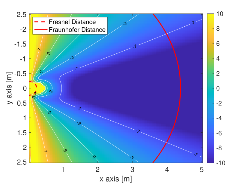
(a) MME-PEB [dB]

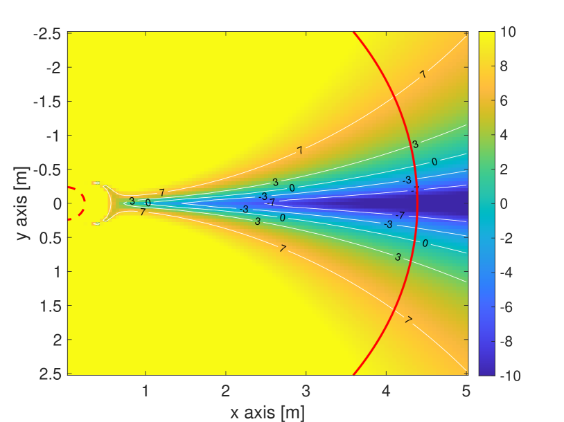
(b) MME-AEB [dB]

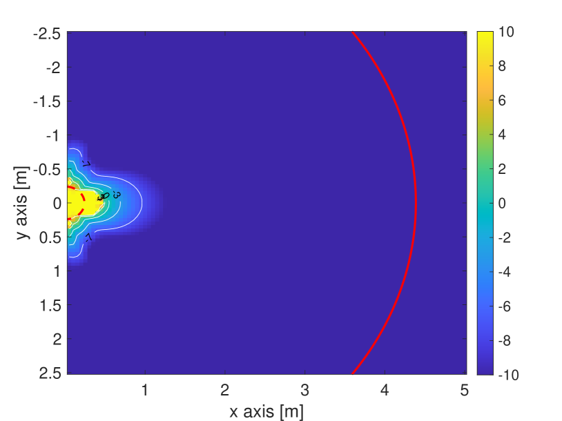
(c) MME-DEB [dB]

Figure 3: Visualization of the model mismatch errors MME-PEB, MME-AEB, and MME-DEB for different UE positions (Digital, $G=1$, $P=20\,\mathrm{dBm}$, $N=64$). We can see that the angle estimation is more affected than delay estimation due to model mismatch.

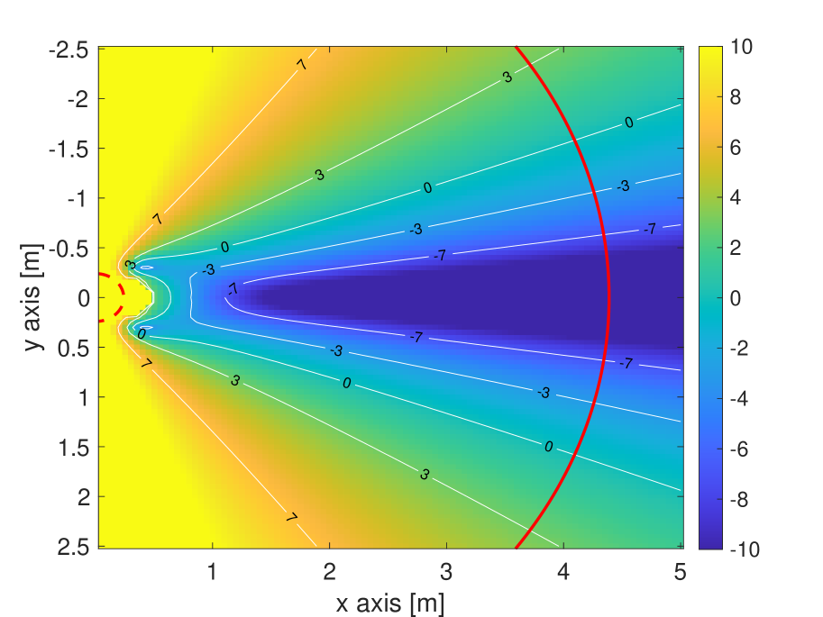
(a) $P=30\,\mathrm{dBm}$

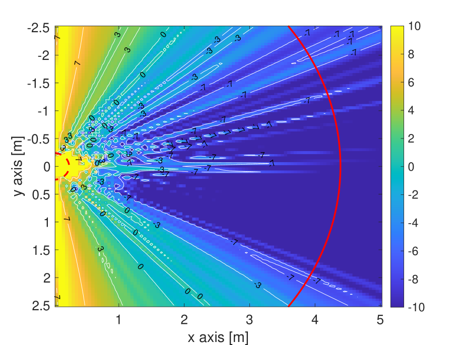
(b) Analog, $G=50$

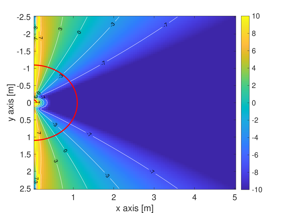
(c) $N=32$

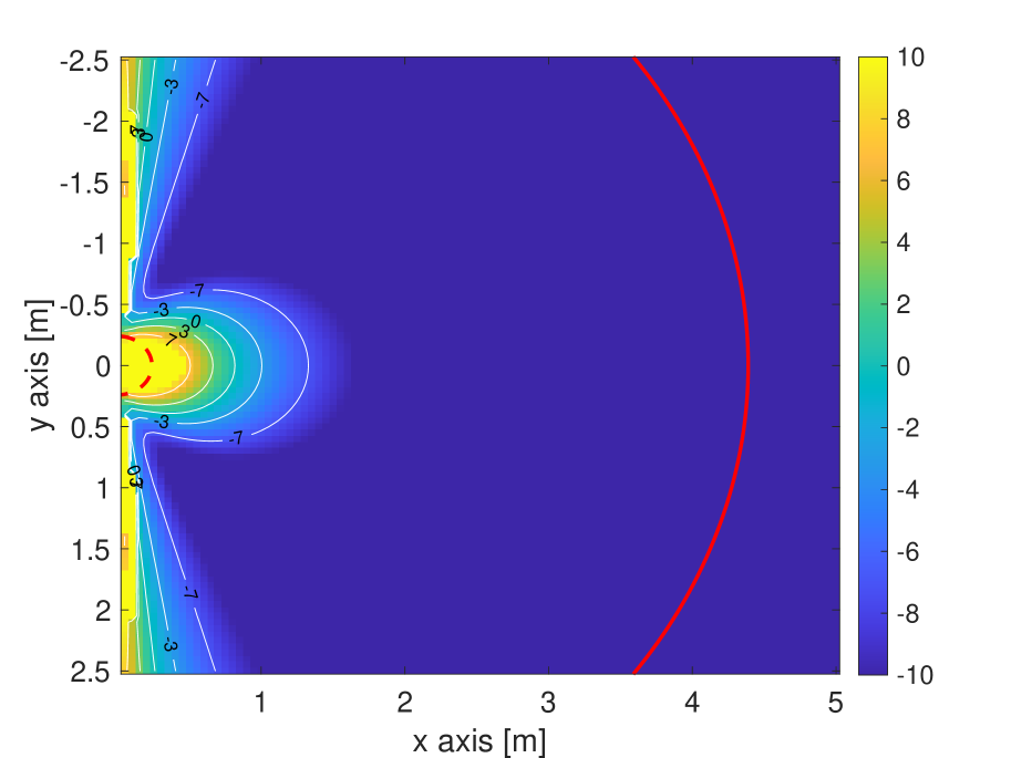
(d) $W=100\,\mathrm{MHz}$

Figure 4: Visualization of relative mismatch error MME-PEB (benchmarked by the MME-PEB in Fig. 3 (a)) for different scenarios: (a) the transmission power $P$ is changed from $10\,\mathrm{dBm}$ to $30\,\mathrm{dBm}$; (b) the array structure is changed to analog array (single RFC) with $\mathcal{G}=50$ transmissions; (c) the array size is changed from 64 to 32; (d) the bandwidth $W$ is changed from $400\,\mathrm{MHz}$ to $100\,\mathrm{MHz}$.

IV-D Evaluation of Model Mismatch Error

We use the proposed MME to visualize the error caused by using a MM. From Fig. 3 (a), we can see that both angle and distance affect the MME. By further decomposing the PEB into a AEB and a DEB, which are shown in Fig. 3 (b) and Fig. 3 (c), it is observed that compared with angle estimation, the delay estimation is less affected by the model mismatch and the $-3\,\mathrm{dB}$ boundary is within $1\,\mathrm{m}$. However, the area MME-AEB $>-3\,\mathrm{dB}$ is much larger than that of the MME-PEB, indicating that the PEB is mainly determined by DEB in the NF.

IV-E MME for Different System Parameters

In Fig. 4, we compare the MME for different scenarios benchmarked by the MME-PEB in Fig. 3 (a). We found out that the mismatch is getting larger with a higher transmission power $P$, as shown in (a). When an analog array is used (and assumes a frequency-independent combiner matrix ${\bf W}_{g}$), the contours are not smooth due to randomness of the combiner matrix, but a similar mismatch pattern compared with a digital array can be seen with sufficient transmissions, as shown in (b). In Fig. 4 (c), the array size is changed from $64$ to $32$, and the area with model mismatch is largely reduced, indicating the effect of SNS and SWM are mitigated. When the bandwidth $W$ is changed from $400\,\mathrm{MHz}$ to $100\,\mathrm{MHz}$, the mismatch is reduced as the MM does not consider the BSE.

V Conclusion

In this work, we derived the LB of a mismatched estimator using MCRB and analyzed the effect of different types of model impairments, namely, SNS, SWM, and BSE. A mme model mismatch error is further defined as the absolute difference between the LB and the CRB of the TM, normalized by the CRB of the TM, which is determined by system parameters. From the analysis, we see that the SNS has the least contribution among all the model impairments, the SWM dominates when the distance is small compared to the array size, and BSE has a more significant effect when the distance is much larger than the array size. The analysis in this work can provide suggestions on the tradeoff between the complexity of channel model and performance loss (by using an approximated, simple model). In future work, we would like to analyze the effect of model mismatch on the 3D position and 3D orientation of an unsynchronized system.

Appendix A

To derive the CRB for the TM, we notice that only channel gain $\alpha_{k,n}$ in (7) is dependent of channel parameters $\rho$ and $\xi$ as $\frac{\partial\alpha_{k,n}}{\partial\rho}=\alpha_{k,n}/\rho$ and $\frac{\partial\alpha_{k,n}}{\partial\xi}=-j\alpha_{k,n}$. The derivative of channel vector with respect to the states $\rho$, $\xi$ and ${\bf p}$ can then be expressed as

$$\frac{\partial h_{k,n}}{\partial\rho} =\frac{h_{k,n}}{\rho},\ \ \ \frac{\partial h_{k,n}}{\partial\xi}=-j{h_{k,n}},$$ (25)

$$\frac{\partial h_{k,n}}{\partial{\bf p}} =\frac{h_{k,n}}{\alpha_{k,n}({\bf p})}\frac{\partial\alpha_{k,n}({\bf p})}{\partial{\bf p}}+\frac{h_{k,n}}{d_{k,n}({\bf p})}\frac{\partial d_{k,n}({\bf p})}{\partial{\bf p}}$$ (26)

$$+\frac{h_{k,n}}{D_{k}({\bf p})}\frac{\partial D_{k}({\bf p})}{\partial{\bf p}},$$

where

$$\frac{\partial\alpha_{k,n}({\bf p})}{\partial{\bf p}} =\alpha\frac{\lambda_{k}}{\lambda_{c}}\left(\frac{{\bf p}}{\|{\bf p}\|\|{\bf p}-{\bf b}_{n}\|}-\frac{({\bf p}-{\bf b}_{n})\|{\bf p}\|}{\|{\bf p}-{\bf b}_{n}\|^{3}}\right),$$ (27)

$$\frac{\partial d_{k,n}({\bf p})}{\partial{\bf p}} =-j\frac{2\pi}{\lambda_{k}}d_{k,n}({\bf p})\left(\frac{{\bf p}-{\bf b}_{n}}{\|{\bf p}-{\bf b}_{n}\|}-\frac{{\bf p}}{\|{\bf p}\|}\right),$$ (28)

$$\frac{\partial D_{k}({\bf p})}{\partial{\bf p}} =-j\frac{2\pi}{\lambda_{k}}D_{k}({\bf p})\frac{{\bf p}}{\|{\bf p}\|}.$$ (29)

Based on these derivatives and (13), the FIM of the state parameters can be obtained.

References

- [1] G. Bresson, Z. Alsayed, L. Yu, and S. Glaser, “Simultaneous localization and mapping: A survey of current trends in autonomous driving,” IEEE Trans. Intell. Veh., vol. 2, no. 3, pp. 194–220, Sep. 2017.
- [2] F. Tao, H. Zhang, A. Liu, and A. Y. Nee, “Digital twin in industry: State-of-the-art,” IEEE Trans. Ind. Informat., vol. 15, no. 4, pp. 2405–2415, Oct. 2018.
- [3] Y. Siriwardhana, P. Porambage, M. Liyanage, and M. Ylianttila, “A survey on mobile augmented reality with 5G mobile edge computing: Architectures, applications, and technical aspects,” IEEE Commun. Surveys Tuts., vol. 23, no. 2, pp. 1160–1192, Feb. 2021.
- [4] H. Chen, H. Sarieddeen, T. Ballal, H. Wymeersch, M.-S. Alouini, and T. Y. Al-Naffouri, “A tutorial on terahertz-band localization for 6G communication systems,” Accepted for publication in IEEE Commun. Surveys Tuts. arXiv preprint arXiv:2110.08581, 2022.
- [5] A. Shahmansoori, G. E. Garcia, G. Destino, G. Seco-Granados, and H. Wymeersch, “Position and orientation estimation through millimeter-wave MIMO in 5G systems,” IEEE Trans. Wireless Commun., vol. 17, no. 3, pp. 1822–1835, Dec. 2017.
- [6] Z. Abu-Shaban, X. Zhou, T. Abhayapala, G. Seco-Granados, and H. Wymeersch, “Error bounds for uplink and downlink 3D localization in 5G millimeter wave systems,” IEEE Trans. Wireless Commun., vol. 17, no. 8, pp. 4939–4954, May. 2018.
- [7] R. Mendrzik, H. Wymeersch, G. Bauch, and Z. Abu-Shaban, “Harnessing NLOS components for position and orientation estimation in 5G millimeter wave MIMO,” IEEE Trans. Wireless Commun., vol. 18, no. 1, pp. 93–107, Oct. 2018.
- [8] A. Elzanaty, A. Guerra, F. Guidi, and M.-S. Alouini, “Reconfigurable intelligent surfaces for localization: Position and orientation error bounds,” IEEE Trans. Signal Process., vol. 69, pp. 5386–5402, Aug. 2021.
- [9] E. De Carvalho, A. Ali, A. Amiri, M. Angjelichinoski, and R. W. Heath, “Non-stationarities in extra-large-scale massive MIMO,” IEEE Wireless Commun., vol. 27, no. 4, pp. 74–80, Aug. 2020.
- [10] J. C. Marinello, T. Abrão, A. Amiri, E. De Carvalho, and P. Popovski, “Antenna selection for improving energy efficiency in XL-MIMO systems,” IEEE Trans. Veh. Technol., vol. 69, no. 11, pp. 13 305–13 318, Sep. 2020.
- [11] J. Tan and L. Dai, “Wideband beam tracking in THz massive MIMO systems,” IEEE J. Sel. Areas Commun., vol. 39, no. 6, pp. 1693–1710, Apr. 2021.
- [12] S. Tarboush, H. Sarieddeen, H. Chen, M. H. Loukil, H. Jemaa, M.-S. Alouini, and T. Y. Al-Naffouri, “Teramimo: A channel simulator for wideband ultra-massive mimo terahertz communications,” IEEE Trans. Veh. Technol., vol. 70, no. 12, pp. 12 325–12 341, Oct. 2021.
- [13] A. Guerra, F. Guidi, D. Dardari, and P. M. Djurić, “Near-field tracking with large antenna arrays: Fundamental limits and practical algorithms,” IEEE Trans. Signal Process., vol. 69, pp. 5723–5738, Aug. 2021.
- [14] M. Rahal, B. Denis, K. Keykhosravi, F. Keskin, B. Uguen, and H. Wymeersch, “Constrained RIS phase profile optimization and time sharing for near-field localization,” in IEEE Veh. Technol. Conf. (VTC), 2022.
- [15] O. Rinchi, A. Elzanaty, and M.-S. Alouini, “Compressive near-field localization for multipath RIS-aided environments,” IEEE Commun. Lett., Feb. 2022.
- [16] L. Le Magoarou, A. Le Calvez, and S. Paquelet, “Massive MIMO channel estimation taking into account spherical waves,” in Proc. IEEE Int. Workshop Signal Process. Adv. Wireless Commun. (SPAWC), 2019.
- [17] S. Fortunati, F. Gini, M. S. Greco, and C. D. Richmond, “Performance bounds for parameter estimation under misspecified models: Fundamental findings and applications,” IEEE Signal Process. Mag., vol. 34, no. 6, pp. 142–157, Nov. 2017.
- [18] B. Friedlander, “Localization of signals in the near-field of an antenna array,” IEEE Trans. Signal Process., vol. 67, no. 15, pp. 3885–3893, Jun. 2019.
- [19] C. A. Balanis, Antenna theory: Analysis and design. John wiley & sons, 2016.
- [20] E. Björnson and L. Sanguinetti, “Power scaling laws and near-field behaviors of massive MIMO and intelligent reflecting surfaces,” IEEE Open J. Commun., vol. 1, pp. 1306–1324, Sep. 2020.
- [21] H. Chen, S. Aghdam, F. Keskin, Y. Wu, S. Lindberg, A. Wolfgang, U. Gustavsson, T. Eriksson, and H. Wymeersch, “MCRB-based performance analysis of 6G localization under hardware impairments,” in Proc. IEEE Int. Conf. Commun. (ICC) workshop, 2022.
- [22] J. Nocedal and S. Wright, Numerical optimization. Springer Science & Business Media, 2006.
- [23] H. Chen, “Radio Localization Matlab Code [Github Repository],” https://github.com/chenhui07c8/Radio_Localization, May. 2022.