$f(R)$-Gravity Generated Post-inflationary Eras and their Effect on Primordial Gravitational Waves

Abstract

In this work we shall consider the effects of a geometrically generated post-inflationary era on the energy spectrum of the primordial gravitational waves. Specifically, we shall consider a post-inflationary constant equation of state era, generated by the synergistic effect of $f(R)$ gravity and of radiation and matter perfect fluids. Two cases of interest shall be studied, one with equation of state parameter $w=-1/3$, in which case the Universe neither accelerates nor decelerates, and one with $w=0$ so an early matter domination era. For the evaluation of the inflationary observational indices which is relevant for the calculation of the gravitational waves energy spectrum, we also took into account the effects of the constant equation of state parameter era, on the $e$-foldings number. In both the $w=-1/3$ and $w=0$ cases, the energy spectrum of the primordial gravitational waves is amplified, but for the $w=0$ case, the effect is stronger.

I Introduction

Inflation is one of the most important theoretical proposals for the early Universe inflation1 ; inflation2 ; inflation3 ; inflation4 , since it solves successfully all the shortcomings of the standard Big Bang cosmology. However, to date there is no hint that inflation occurred primordially, only constraints coming from Cosmic Microwave Background (CMB) experiments, like the latest Planck 2018 collaboration Planck:2018vyg . The occurrence of the inflationary era can be confirmed in two ways, either by observing the so-called $B$-modes in the CMB temperature fluctuations, or by directly observing the stochastic primordial tensor perturbation background in future experiments Hild:2010id ; Baker:2019nia ; Smith:2019wny ; Crowder:2005nr ; Smith:2016jqs ; Seto:2001qf ; Kawamura:2020pcg ; Bull:2018lat , see also LISACosmologyWorkingGroup:2022jok for the latest updates for cosmological studies related to the LISA mission. So far the CMB experiments have not yielded any hints of inflation, however the stage 4 CMB experiments CMB-S4:2016ple ; SimonsObservatory:2019qwx may observe the $B$-modes of inflation directly on the CMB temperature fluctuations. All these experiments are highly anticipated by the theoretical physics, astrophysics and cosmology societies and will provide sensational results. The stage 4 CMB experiments thus, will directly verify the existence of the inflationary era via the direct detection of the $B$-modes (curl modes) of inflation on the CMB radiation temperature and polarization anisotropies. However, the CMB merely probes modes with wavenumbers $k<0.62$ Mpc^-1, and thus primordial modes with larger wavenumbers cannot be probed by the CMB temperature fluctuations, since the CMB itself probes linear modes with wavelength $\lambda$ from $10$ Mpc to $10^{4}$ Mpc. Beyond that, non-linear perturbation theory is needed, thus the CMB cannot reach the modes which became subhorizon immediately after the inflationary era during the reheating era. These modes which have wavelength below $10$ Mpc, are basically subhorizon modes, which exited the Hubble horizon first during the inflationary era, and reentered the horizon first, after inflation ended, thus became subhorizon modes during the first stages of the reheating era and during the subsequent radiation domination era. These tensor modes basically constitute the primordial gravitational waves, and there exists a vast literature on the theoretical aspects of the subject, see for example, Kamionkowski:2015yta ; Denissenya:2018mqs ; Turner:1993vb ; Boyle:2005se ; Zhang:2005nw ; Schutz:2010xm ; Sathyaprakash:2009xs ; Caprini:2018mtu ; Arutyunov:2016kve ; Kuroyanagi:2008ye ; Clarke:2020bil ; Kuroyanagi:2014nba ; Nakayama:2009ce ; Smith:2005mm ; Giovannini:2008tm ; Liu:2015psa ; Zhao:2013bba ; Vagnozzi:2020gtf ; Watanabe:2006qe ; Kamionkowski:1993fg ; Giare:2020vss ; Kuroyanagi:2020sfw ; Zhao:2006mm ; Nishizawa:2017nef ; Arai:2017hxj ; Bellini:2014fua ; Nunes:2018zot ; DAgostino:2019hvh ; Mitra:2020vzq ; Kuroyanagi:2011fy ; Campeti:2020xwn ; Nishizawa:2014zra ; Zhao:2006eb ; Cheng:2021nyo ; Nishizawa:2011eq ; Chongchitnan:2006pe ; Lasky:2015lej ; Guzzetti:2016mkm ; Ben-Dayan:2019gll ; Nakayama:2008wy ; Capozziello:2017vdi ; Capozziello:2008fn ; Capozziello:2008rq ; Cai:2021uup ; Cai:2018dig ; Odintsov:2021kup ; Benetti:2021uea ; Lin:2021vwc ; Zhang:2021vak ; Odintsov:2021urx ; Pritchard:2004qp ; Zhang:2005nv ; Baskaran:2006qs ; Oikonomou:2022xoq ; Odintsov:2022cbm ; Odintsov:2022sdk ; Kawai:2017kqt ; Odintsov:2022hxu ; Gao:2019liu . The era in which the primordial tensor modes became subhorizon, namely the reheating era, is basically unknown to us, and the only way to probe this era is via stochastic gravitational wave experiments Hild:2010id ; Baker:2019nia ; Smith:2019wny ; Crowder:2005nr ; Smith:2016jqs ; Seto:2001qf ; Kawamura:2020pcg ; Bull:2018lat . The primordial gravitational waves will offer us insights, since these are affected by numerous effects, like the matter content of the Universe at horizon reentry, by the total equation of state of the Universe at horizon reentry, by the number of massive and massless particles at horizon reentry and so on. All these effects will have direct impact on the stochastic gravitational wave background, and thus will give us insights on these high energy physics phenomena. Also supersymmetry breaking can also be probed via the stochastic gravitational background, since if a huge damping occurs for a specific frequency range, this means that some particles obtained masses and supersymmetry broke at that frequency range. This is a rather sensational feature. Finally, let us note that the lowest frequency mode that is probed by the CMB experiments corresponds to the tensor mode that reenters the Hubble horizon today, and thus the maximum frequency that can be reached by primordial gravitational waves spectrum is $f_{max}\sim 1$GHz Giovannini:2008tm . The physics in the frequency range $f_{BBN}<f<f_{max}$ (where $f_{BBN}$ is the frequency corresponding to the Big Bang Nucleosynthesis)is unknown to us, hence the primordial gravitational waves will actually reveal new information related to several physical features of this unknown to us era, not up to $f_{max}$ of course, but for frequencies with maximum values several Hz.

Modified gravity in its various forms, can also describe successfully inflation reviews1 ; reviews2 ; reviews3 ; reviews4 ; reviews5 ; reviews6 . The most profound modified gravity theory is $f(R)$ gravity Nojiri:2003ft ; Capozziello:2005ku ; Hwang:2001pu ; Cognola:2005de ; Song:2006ej ; Faulkner:2006ub ; Olmo:2006eh ; Sawicki:2007tf ; Faraoni:2007yn ; Carloni:2007yv ; Nojiri:2007as ; Deruelle:2007pt ; Appleby:2008tv ; Dunsby:2010wg , can describe inflation and dark energy in a unified way, see for example the pioneer work Nojiri:2003ft . With regard to the stochastic inflationary gravitational wave background, if a signal is detected, this will really be intriguing theoretically. This is because most “traditional” theories of standard inflation, like $f(R)$ gravity and single scalar field theories, predict an undetectable energy spectrum of primordial gravitational waves. Thus if a signal is detected, one possibility of interpreting the result is that these fundamental theories are excluded. Another perspective is that it is possible that alternative evolution scenarios took place post-inflationary. In this line of research, in this article we aim to point out that if post-inflationary a short lasting $f(R)$ gravity generated era with constant Equation of State (EoS) parameter took place, then the predicted energy spectrum of the primordial gravitational waves is significantly enhanced. This post-inflationary era will be generated synergistically by $f(R)$ gravity in the presence of matter and radiation perfect fluids. We shall be interested to two distinct constant EoS parameters, with $w=-1/3$ and $w=0$. The first corresponds to a state that the Universe neither accelerates nor decelerates, with $\ddot{a}=0$, while the second case corresponds to an early matter domination era. As we show, in both cases, the predicted energy spectrum of the primordial gravitational waves is significantly enhanced, with the $w=0$ case producing a slightly higher energy spectrum.

This paper is organized as follows: In section II, we present the standard features of inflationary $f(R)$ gravity theories. Also we discuss how a constant EoS post-inflationary era can be realized by $f(R)$ gravity in the presence of perfect matter fluids. Moreover, we show how the constant EoS short lasting post-inflationary era may affect the duration of the inflationary era. In section III we calculate the energy spectrum of the primordial gravitational waves, for both the $w=-1/3$ and $w=0$ cases, and we show that the predicted signal is detectable by most of the future gravitational wave experiments, if the reheating temperature is large enough. Finally, the conclusions follow at the end of the article.

II Inflation and Post-inflation Evolution with $f(R)$ Gravity

As we mentioned in the introduction, our current perception of our Universe indicates that the Universe went through four distinct phases, the inflationary era, followed by the obscured reheating era which consists partially from the radiation domination era, followed by the matter and dark energy eras. To date we have theoretical ideas of what drives inflation and all the post-inflationary eras, but not clear-cut facts. Therefore, if the inflationary and the dark energy eras are controlled by modified gravity, there is no reason why modified gravity should not control the rest of the cosmological eras, synergistically though with the matter and radiation perfect fluids. In this line of research, in this paper we shall assume that $f(R)$ gravity actually controls entirely or synergistically all cosmological eras, and the full form of it has the following approximate behavior,

$$f(R)=\left\{\begin{array}[]{ccc}R+\frac{R^{2}}{6M^{2}}&R\sim R_{I}\,,\\ F_{w}(R)&R\sim R_{PI}\ll R_{I}\,,\\ F_{DE}(R)&R\sim R_{0}\ll R_{PI}\,,\\ \end{array}\right.$$

where $R_{I}$ is the curvature scale of inflation, at the first horizon crossing at the beginning of inflation when the comoving mode $k$ leaves the Hubble horizon primordially. Also $R_{PI}$ is the curvature scale during the early post-inflationary era, right after inflation ends. Finally, $R_{0}$ is the curvature at present day, so it is basically equal to the present day cosmological constant. The functional forms of $F_{w}(R)$ and $F_{DE}(R)$ shall be specified later on. Specifically, the function $F_{w}(R)$ will generate a post-inflationary era with an EoS parameter $w$ which is a constant and we shall specify it shortly. The function $F_{DE}(R)$ is some conveniently chosen $f(R)$ gravity which can produce a viable late-time phenomenology. Also, from the above relation it is apparent that the inflationary era is controlled by an $R^{2}$ gravity. Note that during the inflationary era, the matter and radiation perfect fluids are neglected, but post-inflationary they cannot be neglected. So both $F_{w}(R)$ and $F_{DE}(R)$ synergistically with the matter and radiation perfect fluids, control the evolution of the Universe.

Let us now use the metric $f(R)$ gravity formalism to find $F_{w}(R)$. Consider the $f(R)$ gravity action in the presence of perfect matter fluids,

$$\mathcal{S}=\frac{1}{2\kappa^{2}}\int\mathrm{d}^{4}x\sqrt{-g}\,f(R)+\mathcal{S}_{m},$$ (1)

where $\kappa^{2}$ being equal to $\kappa^{2}=8\pi G=\frac{1}{M_{p}^{2}}$, with $G$ is Newton’s constant, and $M_{p}$ denotes the reduced Planck mass. We shall use the metric formalism, so upon varying the gravitational action with respect to the metric tensor, we obtain the field equations,

$$f_{R}(R)R_{\mu\nu}(g)-\frac{1}{2}f(R)g_{\mu\nu}-\nabla_{\mu}\nabla_{\nu}f_{R}(R)+g_{\mu\nu}\square f_{R}(R)=0\kappa^{2}T_{\mu\nu}^{m}\,,$$ (2)

where $T_{\mu\nu}^{m}$ stands for the energy momentum tensor of the matter and radiation perfect fluids, and also $f_{R}=\frac{\mathrm{d}f}{\mathrm{d}R}$. Assuming that the geometric background is that of a flat Friedmann-Robertson-Walker (FRW) spacetime, the Friedmann equation is written,

$$-18\left(4H(t)^{2}\dot{H}(t)+H(t)\ddot{H}(t)\right)f_{RR}(R)+3\left(H^{2}(t)+\dot{H}(t)\right)f_{R}-\frac{f(R)}{2}+\kappa^{2}\left(\rho_{m}+\rho_{r}\right)=0\,,$$ (3)

with $\rho_{m}$, $\rho_{r}$ denoting the energy density of the cold dark matter and of the radiation perfect fluids respectively. As we mentioned, we shall assume that post-inflationary, for a short period of time, the Universe has a constant EoS parameter $w$, thus the total effective pressure $p_{eff}$ and the total energy density $\rho_{eff}$, satisfy $p_{eff}=w\rho_{eff}$. Thus the scale factor for this short post-inflationary period of time is,

$$a(t)=a_{end}\,t^{\frac{2}{3(1+w)}}\,,$$ (4)

where $a_{end}$ is the scale factor at the end of the inflationary era. Let us find which $f(R)$ gravity can generate the evolution (4) in the presence of matter and radiation perfect fluids. We shall employ the reconstruction techniques of Ref. Nojiri:2009kx which are based on using the $e$-foldings number as a dynamical variable,

$$e^{-N}=\frac{a_{i}}{a}\,,$$ (5)

with $a_{i}$ being some initial value of the scale factor. In terms of the $e$-foldings number $N$, the Friedmann equation becomes,

$$-18\left[4H^{3}(N)H^{\prime}(N)+H^{2}(N)(H^{\prime})^{2}+H^{3}(N)H^{\prime\prime}(N)\right]f_{RR}(R)+3\left[H^{2}(N)+H(N)H^{\prime}(N)\right]f_{R}(R)-\frac{f(R)}{2}+\kappa^{2}\rho=0\,,$$ (6)

with $\rho=\rho_{m}+\rho_{r}$. Upon introducing the function, $G(N)=H^{2}(N)$, we can write the Ricci scalar as follows,

$$R=3G^{\prime}(N)+12G(N)\,.$$ (7)

Thus by using a given scale factor, for example that of Ref. (4), we can solve everything with respect to the cosmic time, find $t=t(a)$ and by using (5) in conjunction with (7) we can find the function $N(R)$. Thus by replacing in Eq. (6), we end up with the following second order differential equation,

$$-9G(N(R))\left[4G^{\prime}(N(R))+G^{\prime\prime}(N(R))\right]f_{RR}(R)+\left[3G(N)+\frac{3}{2}G^{\prime}(N(R))\right]f_{R}(R)-\frac{f(R)}{2}+\kappa^{2}\left(\rho_{m}+\rho_{r}\right)=0\,,$$ (8)

with $G^{\prime}(N)=\mathrm{d}G(N)/\mathrm{d}N$ and $G^{\prime\prime}(N)=\mathrm{d}^{2}G(N)/\mathrm{d}N^{2}$. Upon solving the above equation, one can specify the function $f(R)$ which realizes the given scale factor. Let us apply the method for the scale factor (4). For the scale factor (4) the function $G(N)$ takes the form,

$$G(N)=\frac{4e^{-3N(w+1)}}{9(w+1)^{2}}\,,$$ (9)

with $a_{r}=1$ for convenience. Combining Eqs. (7) and (9), we have,

$$N=\frac{\log\left(\frac{4(1-3w)}{3R(w+1)^{2}}\right)}{3(w+1)}.$$ (10)

Taking the above into account, combined with the fact that

$$\rho_{tot}=\sum_{i}\rho_{i0}a_{0}^{-3(1+w_{i})}e^{-3N(R)(1+w_{i})}\,,$$ (11)

the Friedmann equation (8), takes the form,

$$a_{1}R^{2}\frac{\mathrm{d}^{2}f(R)}{\mathrm{d}R^{2}}+a_{2}R\frac{\mathrm{d}f(R)}{\mathrm{d}R}-\frac{f(R)}{2}+\sum_{i}S_{i}R^{\frac{3(1+w_{i})}{3(1+w)}}=0\,,$$ (12)

with the index “i” taking the values $i=(r,m)$ with $i=r$ corresponding to radiation and $i=m$ corresponding to cold dark matter perfect fluids. Also $a_{1}$ and $a_{2}$, $S_{i}$ and $A$ are defined as follows,

$$a_{1}=\frac{3(1+w)}{4-3(1+w)},\,\,\,a_{2}=\frac{2-3(1+w)}{2(4-3(1+w))},\,\,\,S_{i}=\frac{\kappa^{2}\rho_{i0}a_{0}^{-3(1+w_{i})}}{[3A(4-3(1+w))]^{\frac{3(1+w_{i})}{3(1+w)}}},\,\,\,A=\frac{4}{3(w+1)}$$ (13)

The solution of (12) is actually the $f(R)$ gravity which generates the post-inflationary evolution (4), which we denoted $F_{w}(R)$ and it is,

$$F_{w}(R)=\left[\frac{c_{2}\rho_{1}}{\rho_{2}}-\frac{c_{1}\rho_{1}}{\rho_{2}(\rho_{2}-\rho_{1}+1)}\right]R^{\rho_{2}+1}+\sum_{i}\left[\frac{c_{1}S_{i}}{\rho_{2}(\delta_{i}+2+\rho_{2}-\rho_{1})}\right]R^{\delta_{i}+2+\rho_{2}}-\sum_{i}B_{i}c_{2}R^{\delta_{i}+\rho_{2}}+c_{1}R^{\rho_{1}}+c_{2}R^{\rho_{2}}\,,$$ (14)

with $c_{1},c_{2}$ being integration constants, and also we introduced $\delta_{i}$ and $B_{i}$,

$$\delta_{i}=\frac{3(1+w_{i})-23(1+w)}{3(1+w)}-\rho_{2}+2,\,\,\,B_{i}=\frac{S_{i}}{\rho_{2}\delta_{i}}\,,$$ (15)

with $i=(r,m)$. Recall that we have assume that,

$$f(R)=\left\{\begin{array}[]{ccc}R+\frac{R^{2}}{6M^{2}}&R\sim R_{I}\,,\\ F_{w}(R)&R\sim R_{PI}\ll R_{I}\,,\\ F_{DE}(R)&R\sim R_{0}\ll R_{PI}\,,\\ \end{array}\right.$$

so post-inflationary, the $f(R)$ gravity is given by $F_{w}(R)$ given in Eq. (14). Regarding the late-time era, the $f(R)$ gravity can be of power-law type such as the one studied in Ref. Odintsov:2021kup , which we will use too in this work, and it is,

$$F_{DE}(R)=-\gamma\Lambda\Big{(}\frac{R}{3m_{s}^{2}}\Big{)}^{\delta}\,,$$ (16)

with $m_{s}$ in Eq. (16) being defined as $m_{s}^{2}=\frac{\kappa^{2}\rho_{m}^{(0)}}{3}$, and also $\rho_{m}^{(0)}$ is the energy density of cold dark matter at present day. Moreover, the parameter $\delta$ takes values in the interval $0<\delta<1$, and $\gamma$ is a dimensionless parameter, while $\Lambda$ is the present day cosmological constant. The model (16) generates a viable dark energy era, as it was proven in detail in Odintsov:2021kup . Thus during the inflationary era the evolution is driven by the $R^{2}$ model, while post-inflationary and for a short period, the evolution is described by $F_{w}(R)$ given in Eq. (14), while at late times the evolution is driven by $F_{DE}(R)$ given in Eq. (16). Such a description describes the evolution in different patches, so an effective model which can potentially describe in a unified way the different evolution patches we described above is,

$$f(R)=e^{-\frac{\Lambda}{R}}\left(R+\frac{R^{2}}{6M^{2}}\right)+e^{-\frac{R}{\Lambda}}\tanh\left(\frac{R-R_{PI}}{\Lambda}\right)F_{DE}(R)+e^{-\frac{R}{\Lambda}}\tanh\left(\frac{R-R_{0}}{\Lambda}\right)\left(F_{w}(R)-R-\frac{R^{2}}{6M^{2}}\right)\,,$$ (17)

where $R_{PI}$ is the curvature during the era with EoS parameter $w$ and also $R_{0}$ stands for the curvature at present day. We need to note that the above model is a theoretical approximation of the full functional form of the $f(R)$ gravity, not an exact solution of the Friedmann equation. Hence in the way given above, one needs to have available the full functional form of the scale factor, which is simply impossible to find. However, the different patches of the $f(R)$ gravity can satisfy the Friedmann equation (6) or equivalently (3), given the scale factor. For example, when $R\sim R_{PI}$, the effective model (17) yields $f(R)\sim F_{w}(R)$ and this approximate form satisfies exactly the Friedmann equations (6) or equivalently (3) for the scale factor (4). In fact the solution (14) is an exact solution of the Friedmann equation (6) for the scale factor being (4), in the presence of matter and radiation fluids.

Of course the above model is an effective description which realizes in a unified way the different evolutionary patches we described previously, so many other models may describe such a behavior. The model (17) is just an example, out of many which may effective describe the different evolution patches we described previously. In all the cases though, the total $f(R)$ gravity must satisfy several theoretical constraints and also the leading order form of the $f(R)$ gravity at present time must respect the solar system constraints.

Regarding the theoretical constraints that must be satisfied by any $f(R)$ gravity at all eras, these are, reviews1 ,

$$f^{\prime}(R)>0\,,\,\,\,f^{\prime\prime}(R)>0\,,$$ (18)

for $R>R_{0}$, with $R_{0}$ being the curvature of the Universe at present day. Hence, the model and every other model that can describe the different patches of the $f(R)$ gravity quoted below Eq. (15), must satisfy the viability criteria (18) for all curvatures up to $R\sim R_{I}$ with $R_{I}\sim 12H_{I}^{2}$, and with $H_{I}$ being the inflationary scale, which is $H_{I}\sim 10^{13}\,$GeV in the low scale inflationary scenarios. Let us see whether the effective model (17) satisfies the viability criteria (18). For $R\sim R_{PI}$, so when the Universe is during the post-inflationary $w$-era, we have $\tanh\left(\frac{R-R_{PI}}{\Lambda}\right)\sim 0$, and in addition, $\Lambda/R_{PI}\sim 0$ thus $e^{-\frac{\Lambda}{R}}\sim 1$, and moreover $\tanh\left(\frac{R-R_{0}}{\Lambda}\right)\simeq 1$ since $R_{PI}\gg R_{0}$, hence the $f(R)$ gravity is approximately described by $f(R)\simeq F_{w}(R)$. We have checked these constraints numerically for the form of $F_{w}(R)$ we found in Eq. (14) previously, and viability constraints (18) are satisfied for both the values of $w$ we shall use, namely $w=-1/3$ and $w=0$. Also it must be noted that the free chosen constants $c_{1}$ and $c_{2}$ must take negative values in order for the viability criteria (18) to be satisfied. Furthermore when $R\sim R_{0}$ at present day, then $\tanh\left(\frac{R-R_{0}}{\Lambda}\right)\simeq 0$, thus the $f(R)$ gravity at present day is at leading order $f(R)=R+\frac{R^{2}}{6M^{2}}+F_{DE}(R)$ with the functional form of $F_{DE}(R)$ being quoted in Eq. (16). At late times, the viability criteria of the model $f(R)=R+\frac{R^{2}}{6M^{2}}+F_{DE}(R)$ have been investigated in Ref. Odintsov:2020nwm (see figure 5 of Ref. Odintsov:2020nwm ) for both the late-time era and also for the case that $R\sim 12H_{I}^{2}$ with $H_{I}$ being the inflationary scale. In the latter case we have $R\sim 12H_{I}^{2}$ and $f(R)\sim R+\frac{R^{2}}{6M^{2}}$ so for $H_{I}\sim 10^{13}\,$GeV we have (see also Odintsov:2020nwm below Eq. (47)) $f^{\prime\prime}(R)\sim 2.15\times 10^{-28}\,$eV^-1 and $f^{\prime}(R)\sim 3.59$. Thus the viability conditions are satisfied, and also regarding the solar system tests, the model at late times $f(R)=R+\frac{R^{2}}{6M^{2}}+F_{DE}(R)$ is known to pass the solar system constraints, see for example the review reviews1 .

Essential for the calculation of the primordial gravitational waves energy spectrum, are the tensor-to-scalar ratio and the tensor spectral index. In most cases in the literature, post-inflationary the Universe is described by the radiation era which is followed by the matter domination era. In these cases, the modes which exited the horizon first during the beginning of inflation, are affected in the standard way described in the literature, via the $e$-foldings number which measures the duration of the inflationary era, so usually $N\sim 60$. However, even a short post-inflationary era with general EoS parameter $w$ different from that of radiation, will have a direct effect on the $e$-foldings number. Specifically, the $e$-foldings number for a primordial mode $k$ which exited the horizon during the first horizon crossing at the beginning of inflation, is given by Adshead:2010mc ,

$$\frac{a_{k}H_{k}}{a_{0}H_{0}}=e^{-N}\frac{H_{k}a_{end}}{a_{reh}H_{reh}}\frac{H_{reh}a_{reh}}{a_{eq}H_{eq}}\frac{H_{eq}a_{eq}}{a_{0}H_{0}}\,,$$ (19)

where $a_{k}$ and $H_{k}$ are the scale factor and the Hubble rate at the moment in which the primordial mode $k$ exits the horizon at the beginning of the inflationary era, $a_{end}$ is the scale factor at the end of inflation, $a_{reh}$ and $H_{reh}$ are the scale factor and the Hubble rate at the end of the reheating era. Also, $a_{eq}$ and $H_{eq}$ are the scale factor and the Hubble rate at the matter-radiation equality, and $a_{0}$ and $H_{0}$ are the scale factor and the Hubble rate at present day. Assuming that post-inflationary, right after the end of the inflationary era, the effective EoS parameter is constant $w$, we easily obtain that,

$$\ln\left(\frac{a_{end}H_{end}}{a_{reh}H_{reh}}\right)=-\frac{1+3w}{6(1+w)}\ln\left(\frac{\rho_{reh}}{\rho_{end}}\right)\,,$$ (20)

where $H_{end}$ is the Hubble rate at the end of inflation and $\rho_{end}$ and $\rho_{reh}$ are the energy density of the Universe at the end of the inflationary era and of the reheating era respectively. Also for deriving the relation of Eq. (20) we assumed that at the time instances at the end of inflation and at the end of the reheating era, the effective EoS parameter is $w$. If post-inflationary the Universe is described by a constant effective EoS parameter $w$ short era, followed by standard radiation and matter domination eras, the $e$-foldings number is easily found to be Adshead:2010mc ,

$$N=56.12-\ln\left(\frac{k}{k_{*}}\right)+\frac{1}{3(1+w)}\ln\left(\frac{2}{3}\right)+\ln\left(\frac{\rho_{k}^{1/4}}{\rho_{end}^{1/4}}\right)+\frac{1-3w}{3(1+w)}\ln\left(\frac{\rho_{reh}^{1/4}}{\rho_{end}^{1/4}}\right)+\ln\left(\frac{\rho_{k}^{1/4}}{10^{16}\mathrm{GeV}}\right)\,,$$ (21)

where $\rho_{k}$ is the energy density of the Universe at the beginning of the inflationary era, when the mode $k$ exited the horizon. Also the pivot scale $k_{*}$ is $k_{*}=0.05$Mpc^-1 and in addition a major assumption we shall take into account in the following is that effective degrees of freedom of particles during inflation, until the end of the radiation domination era is constant. Thus we neglect mechanisms which may effectively change the effective degrees of freedom during reheating, for example supersymmetry breaking or other mechanisms. In principle, the neglected cases can also be dealt in a similar way to that we shall demonstrate, with slight changes incorporated in the effective degrees of freedom parameter $g_{*}$ which enters in the general relation for all energy densities and the corresponding temperature $\rho=\frac{\pi^{2}}{30}g_{*}T^{4}$. With this assumption, we can easily rewrite Eq. (21) in terms of the corresponding temperatures instead of the energy densities.

Let us now proceed to quantify our findings in terms of several possible scenarios for the constant $w$ short post-inflationary era. As we mentioned, our main assumption is that this short constant $w$ era is generated by $f(R)$ gravity, thus the geometry effectively generates this era. In general, this short era can have any value in the range $-\frac{1}{3}\leq w\leq 1$. For the purposes of this work we shall confine ourselves in two scenarios listed below,

$$\mathrm{Scenario}\,\,I\,:\,\,\mathrm{EoS}\,\,w=-\frac{1}{3}\,\,(\ddot{a}=0)\,,$$ (22)

$$\mathrm{Scenario}\,\,II\,:\,\,\mathrm{EoS}\,\,w=0\,\,(\mathrm{Early}\,\,\,\mathrm{Matter}\,\,\,\mathrm{Domination})\,.$$

The Scenario I corresponds to a short-lasting post-inflationary era with EoS parameter equal to $w=-1/3$, for which the Universe neither accelerates nor decelerates, since $\ddot{a}=0$ for $w=-1/3$. This evolution is known as thermal inflation in the literature Burgess:2005sb . The Scenario II corresponds to an early matter domination era with EoS parameter $w=0$. In both cases, these short post-inflationary eras have geometric origin and are generated by the $f(R)$ gravity $F_{w}(R)$, both in the presence of matter and radiation perfect fluids. The perfect fluids play an also important role, since post-inflationary these cannot be neglected, as in the inflationary case. Thus the synergy of $f(R)$ gravity and matter and radiation perfect fluids gives rise to these $w$-EoS post-inflationary eras. Finally, we shall consider three different reheating temperatures, listed below,

$$\mathrm{High}\,\,\,\mathrm{Reheating}\,\,\,\mathrm{Temperature}:\,\,\,T_{R}=10^{12}\mathrm{GeV}\,,$$ (23)

$$\mathrm{Intermediate}\,\,\,\mathrm{Reheating}\,\,\,\mathrm{Temperature}:\,\,\,T_{R}=10^{7}\mathrm{GeV}\,,$$

$$\mathrm{Low}\,\,\,\mathrm{Reheating}\,\,\,\mathrm{Temperature}:\,\,\,T_{R}=10^{2}\mathrm{GeV}\,.$$

In the literature there exist scenarios which motivate the low-reheating temperature case, in some cases even motivate MeV scale reheating temperatures Hasegawa:2019jsa .

Table 1: Scenario I: EoS $w=-\frac{1}{3}$ ($\ddot{a}$)

Observational Indices and $e$-foldings	$T_{R}=10^{12}$GeV	$T_{R}=10^{7}$GeV	$T_{R}=10^{2}$GeV
$e$-foldings number $N$	63.7413	52.2284	40.7155
Tensor-to-Scalar Ratio $r$	0.00295352	0.00439914	0.00723873
Tensor Spectral Index $n_{T}$	-0.0000615316	-0.0000916488	-0.000150807

Let us now proceed to the evaluation of the observational indices relevant to the calculation of the energy spectrum of the primordial gravitational waves. Specifically, we shall calculate the tensor-to-scalar ratio and the tensor spectral index, for the Scenarios I and II, and for the three distinct reheating temperatures. We shall be interested in modes with $k=0.05$Mpc^-1, which is the pivot scale used in Planck. For $f(R)$ gravity, the tensor-to-scalar ratio is reviews1 ; Odintsov:2020thl ; Odintsov:2021kup ,

$$r=48\epsilon_{1}^{2}\,,$$ (24)

and the tensor spectral index for $f(R)$ gravity is reviews1 ; Odintsov:2020thl ; Odintsov:2021kup ,

$$n_{T}\simeq-2\epsilon_{1}^{2}\,,$$ (25)

where $\epsilon_{1}$ is the first slow-roll index $\epsilon_{1}=-\dot{H}/H^{2}$. Since the inflationary era is controlled by an $R^{2}$ gravity in the present context, the first slow-roll index is $\epsilon_{1}\simeq\frac{1}{2N}$, hence the resulting tensor spectral index is,

$$n_{T}\simeq-\frac{1}{2N^{2}}\,,$$ (26)

while the tensor-to-scalar ratio for the $R^{2}$ model is,

$$r=\frac{12}{N^{2}}\,.$$ (27)

Now the $e$-foldings number is affected by both the reheating temperature and the EoS parameter $w$, as is dictated by relation (21). Hence we will calculate the $e$-foldings number for the two scenarios of Eq. (23) and for the three different reheating temperatures (23). The results for the Scenarios I and II can be found in Tables 1 and 2.

Table 2: Scenario II: EoS $w=0$ (Early Matter Domination)

Observational Indices and $e$-foldings	$T_{R}=10^{12}$GeV	$T_{R}=10^{7}$GeV	$T_{R}=10^{2}$GeV
$e$-foldings number $N$	65.3439	61.5063	57.6687
Tensor-to-Scalar Ratio $r$	0.00281042	0.00317206	0.00360829
Tensor Spectral Index $n_{T}$	-0.0000585503	-0.0000660847	-0.0000751727

For both Scenarios I and II, there exist several mentionable features, for example in both Scenarios I and II for the large reheating temperature case, the $e$-foldings number exceeds $N=60$. Also for the Scenario I, the low reheating temperature case results to a small $e$-foldings number. Finally, for Scenario II, all the $e$-foldings numbers satisfy $N>50$. In the next section we shall use the tensor-to-scalar ratio and the tensor spectral index from Tables 1 and 2, in order to calculate the predicted energy spectrum of the primordial gravitational waves for the $f(R)$ gravity theoretical framework developed in this paper.

III Primordial Gravitational Wave Energy Spectrum Amplification Due to non-canonical $f(R)$ Reheating

In the literature there exist several works on theoretical predictions of the energy spectrum of the primordial gravitational waves Kamionkowski:2015yta ; Denissenya:2018mqs ; Turner:1993vb ; Boyle:2005se ; Zhang:2005nw ; Schutz:2010xm ; Sathyaprakash:2009xs ; Caprini:2018mtu ; Arutyunov:2016kve ; Kuroyanagi:2008ye ; Clarke:2020bil ; Kuroyanagi:2014nba ; Nakayama:2009ce ; Smith:2005mm ; Giovannini:2008tm ; Liu:2015psa ; Zhao:2013bba ; Vagnozzi:2020gtf ; Watanabe:2006qe ; Kamionkowski:1993fg ; Giare:2020vss ; Kuroyanagi:2020sfw ; Zhao:2006mm ; Nishizawa:2017nef ; Arai:2017hxj ; Bellini:2014fua ; Nunes:2018zot ; DAgostino:2019hvh ; Mitra:2020vzq ; Kuroyanagi:2011fy ; Campeti:2020xwn ; Nishizawa:2014zra ; Zhao:2006eb ; Cheng:2021nyo ; Nishizawa:2011eq ; Chongchitnan:2006pe ; Lasky:2015lej ; Guzzetti:2016mkm ; Ben-Dayan:2019gll ; Nakayama:2008wy ; Capozziello:2017vdi ; Capozziello:2008fn ; Capozziello:2008rq ; Cai:2021uup ; Cai:2018dig ; Odintsov:2021kup ; Benetti:2021uea ; Lin:2021vwc ; Zhang:2021vak ; Odintsov:2021urx ; Pritchard:2004qp ; Zhang:2005nv ; Baskaran:2006qs ; Oikonomou:2022xoq ; Odintsov:2022cbm ; Odintsov:2022sdk and in about fifteen years from now, the experiments will start to yield data. Thus very soon from now, several theoretical frameworks will be put to test. Most of the experiments will probe modes that re-entered the Hubble horizon during the dark era of reheating and during the radiation domination era. In this work we shall be interested in calculating the energy spectrum of the primordial gravitational waves, generated by an underlying $f(R)$ gravity theory which we developed in the previous section. Our main interest is to see the synergistic effect of a short $f(R)$ gravity generated era with constant EoS parameter $w$, in the presence of matter and radiation fluids.

Let us fix the duration of this short $w$-era, and without loss of generality, let us assume that it lasts from the end of inflation, so from temperature $T_{end}\sim 10^{13}$GeV, until $T_{pr}=10^{12}$GeV. Note that the high scale reheating case we discussed in the previous section, corresponds to the same temperature as $T_{pr}=10^{12}$GeV. In order to calculate the exact effect of the constant $w$ $f(R)$ gravity generated era, we need to find the redshifts corresponding to the temperatures $T_{end}$ and $T_{pr}$. Using the relation $T=T_{0}(1+z)$ Garcia-Bellido:1999qrp , with $T_{0}$ being the present day temperature $T_{0}=2.58651\times 10^{-4}$eV, we easily find that the redshift corresponding to $T_{end}$ is $z_{end}=3.86621\times 10^{16}$ while the redshift corresponding to $T_{pr}$ is $z_{pr}=3.86621\times 10^{15}$.

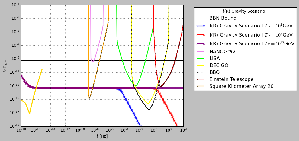
Figure 1: The $h^{2}$-scaled gravitational wave energy spectrum for the $w$-era $f(R)$ gravity, and for the Scenario I. The $f(R)$ gravity curves correspond to $T_{R}=10^{12}$GeV (purple), to $T_{R}=10^{7}$GeV (red) and to (blue) $T_{R}=10^{2}$GeV.

Now let us briefly recall how to calculate the overall effect of $f(R)$ gravity on the energy spectrum of the primordial gravitational waves, from present day at redshift $z=0$ up to the inflationary era. Details on this analysis can be found Odintsov:2021kup . The parameter that quantifies the overall effect of $f(R)$ gravity on the general relativistic waveform is $\alpha_{M}$, defined as,

$$a_{M}=\frac{f_{RR}\dot{R}}{f_{R}H}\,,$$ (28)

and the deformation of the general relativistic waveform is Nishizawa:2017nef ; Arai:2017hxj ,

$$h=e^{-\mathcal{D}}h_{GR}\,,$$ (29)

with $h_{GR}$ being the general relativistic waveform with $a_{M}=0$, and $\mathcal{D}$ being defined as,

$$\mathcal{D}=\frac{1}{2}\int^{\tau}a_{M}\mathcal{H}{\rm d}\tau_{1}=\frac{1}{2}\int_{0}^{z}\frac{a_{M}}{1+z^{\prime}}{\rm dz^{\prime}}\,.$$ (30)

Let us here quote in brief some details regarding the derivation of Eqs. (30)-(32). For more details we refer the reader to Ref. Odintsov:2021kup and more importantly to Ref. Odintsov:2022cbm . The differential equation which is obeyed by the Fourier transformation of the primordial tensor perturbation $h_{ij}$, has the following form,

$$\ddot{h}(k)+\left(3+a_{M}\right)H\dot{h}(k)+\frac{k^{2}}{a^{2}}h(k)=0\,,$$ (31)

where $\alpha_{M}$ is defined as follows,

$$a_{M}=\frac{\dot{Q}_{t}}{Q_{t}H}\,,$$ (32)

and the function $Q_{t}$ is unique for every distinct modified gravity. For a complete list of all the functional forms of $Q_{t}$ and $a_{M}$ we refer the reader to the review Odintsov:2022cbm . Basically, the parameter $a_{M}$ quantifies the overall effect of the modified gravity on the tensor perturbations evolution. For a general $f(R,\phi)$ gravity with action,

$$\mathcal{S}=\int\mathrm{d}^{4}x\sqrt{-g}\Big{(}\frac{f(R,\phi)}{2}-\frac{\omega(\phi)}{2}\partial^{\mu}\phi\partial_{\mu}\phi-V(\phi)\Big{)}\,,$$ (33)

the parameter $Q_{t}$ is $Q_{t}=\frac{1}{\kappa^{2}}\frac{\partial f(R,\phi)}{\partial R}$, where $\kappa=\frac{1}{M_{p}}$, where $M_{p}$ is the reduced Planck mass. Therefore, for a pure $f(R,\phi)$ gravity, the parameter $a_{M}$ has the following form,

$$a_{M}=\frac{\frac{\partial^{2}f}{\partial R\partial\phi}\dot{\phi}+\frac{\partial^{2}f}{\partial R^{2}}\dot{R}}{\frac{\partial f}{\partial R}H}\,,$$ (34)

which reduces to that of Eq. (32) when a pure $f(R)$ gravity is considered, in which case $f(R,\phi)=f(R)$. Using the conformal time $\tau$, the evolution equation (31) is written as,

$$h^{\prime\prime}(k)+\left(2+a_{M}\right)\mathcal{H}h^{\prime}(k)+k^{2}h(k)=0\,,$$ (35)

where the “prime” indicates differentiation with respect to the conformal time $\tau$, and furthermore we also defined $\mathcal{H}=\frac{a^{\prime}}{a}$. The WKB solution of the above differential equation shall now be extracted, considering only subhorizon modes which satisfy Eq. (35). Recall that the subhorizon modes will directly be probed by the future gravitational wave experiments, since these modes became subhorizon modes during the reheating era. Lets consider a WKB solution of the following form $h_{ij}=\mathcal{A}e^{i\mathcal{B}}h_{ij}^{GR}$, describes theories with gravitational wave speed equal to unity in natural units, so in this case the full WKB solution of Eq. (35) is Nishizawa:2017nef ; Arai:2017hxj ,

$$h=e^{-\mathcal{D}}h_{GR}\,,$$ (36)

with $h_{ij}=he_{ij}$, and with $h_{GR}$ denoting the general relativistic waveform which note that it is the solution of the differential equation (35) with $a_{M}=0$. After discussing these important issues, let us proceed to the gravitational wave energy spectrum.

The energy spectrum of the primordial gravitational waves including the effects of $f(R)$ gravity is Boyle:2005se ; Nishizawa:2017nef ; Arai:2017hxj ; Nunes:2018zot ; Liu:2015psa ; Zhao:2013bba ; Odintsov:2021kup ,

$$\Omega_{\rm gw}(f)=e^{-2\mathcal{D}}\times\frac{k^{2}}{12H_{0}^{2}}r\mathcal{P}_{\zeta}(k_{ref})\left(\frac{k}{k_{ref}}\right)^{n_{T}}\left(\frac{\Omega_{m}}{\Omega_{\Lambda}}\right)^{2}\left(\frac{g_{*}(T_{\rm in})}{g_{*0}}\right)\left(\frac{g_{*s0}}{g_{*s}(T_{\rm in})}\right)^{4/3}\left(\overline{\frac{3j_{1}(k\tau_{0})}{k\tau_{0}}}\right)^{2}T_{1}^{2}\left(x_{\rm eq}\right)T_{2}^{2}\left(x_{R}\right)\,,$$

where $k_{ref}=0.002$ Mpc^-1 is the CMB pivot scale, $n_{T}$ is the tensor spectral index and $r$ is the tensor-to-scalar ratio. Thus, the vital element of the evaluation of the energy spectrum is calculating the parameter $\mathcal{D}$. For the evaluation, we need to divide the integration periods to two, with the first being from present day up to redshift $z_{pr}=3.86621\times 10^{15}$ and the second from the redshift $z_{pr}$ up to $z_{end}=3.86621\times 10^{16}$ exactly at the end of the inflationary era. In these two intervals, the dominant $f(R)$ gravity form is different, so the $a_{M}$ parameter defined in (32) is different, and specifically we have,

$$\mathcal{D}=\frac{1}{2}\left(\int_{0}^{z_{pr}}\frac{a_{M_{1}}}{1+z^{\prime}}{\rm dz^{\prime}}+\int_{z_{pr}}^{z_{end}}\frac{a_{M_{2}}}{1+z^{\prime}}{\rm dz^{\prime}}\right)\,,$$ (37)

where the parameters $a_{M_{1}}$ and $a_{M_{2}}$ being evaluated for $f(R)\sim R+f_{DE}(R)$ and $f(R)\sim F_{w}(R)$ respectively. For the first integral, as it was shown Odintsov:2021kup , the contribution is almost zero, so this can be neglected. For the second integral, for the high reheating temperature case, the contribution for $w=-1/3$ is $\int_{z_{pr}}^{z_{end}}\frac{a_{M_{2}}}{1+z^{\prime}}{\rm dz^{\prime}}=-12.434$ and for $w=0$ the contribution is $\int_{z_{pr}}^{z_{end}}\frac{a_{M_{2}}}{1+z^{\prime}}{\rm dz^{\prime}}=-14.5063$. Hence the overall amplification factors are of the order $\mathcal{O}(10^{5})$ and $\mathcal{O}(10^{6})$ respectively. We evaluated the energy spectrum for both the Scenario I ($w=-1/3$) and II ($w=0$) and for all the reheating temperatures, and the results of our analysis appear in Figs. 1 and 2, where we plot the $f(R)$ gravity $h^{2}$-scaled energy spectrum versus the frequency. In the plots the sensitivity curves of most of the future gravitational waves experiments are shown too. We used the three different reheating temperatures and specifically, the purple curve corresponds to the high reheating temperature $T_{R}=10^{12}$GeV, the red curve corresponds to the intermediate reheating temperature $T_{R}=10^{7}$GeV and the blue curve corresponds to the low reheating temperature $T_{R}=10^{2}$GeV.

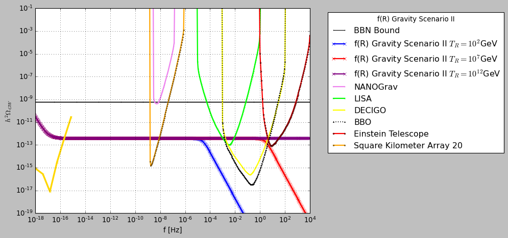
Figure 2: The $h^{2}$-scaled gravitational wave energy spectrum for the $w$-era $f(R)$ gravity, and for the Scenario II. The $f(R)$ gravity curves correspond to $T_{R}=10^{12}$GeV (purple), to $T_{R}=10^{7}$GeV (red) and to (blue) $T_{R}=10^{2}$GeV.

As it can be seen in Figs. 1 and 2, in both cases for Scenarios I and II, the low-reheating temperature signal will be undetectable from some future experiments, and also the intermediate reheating temperature case will be undetectable by the Einstein telescope. Finally let us note that the signal produced by the Scenario II is larger compared to that of Scenario I.

In conclusion, the results indicate that even a short period with EoS parameters $w=-1/3$ and $w=0$ generated by $f(R)$ gravity synergistically with matter and radiation fluids, will be detectable by future gravitational wave experiments. This result changes our perspective on primordial gravitational waves experiments, since it shows that even $f(R)$ gravity may lead to detectable primordial gravitational waves signals.

Finally, let us briefly discuss the scale of the reheating temperature. Basically, this era is known in cosmology as the dark age, since we know nothing about the reheating and the subsequent radiation domination era. In contrast to the post-recombination era for $z>1100$ which we know very well via the CMB, to date we have only hints that the reheating era existed, since after inflation the Universe was too cold and some mechanism should heat up the Universe in order for it to proceed to the formation of galaxies. This is the reheating mechanism after inflation, but we do not know the essential features of this era and the subsequent radiation domination era. We know that the reheating temperature should be smaller than the low scale inflation scenario temperature, so smaller than $T\leq 10^{12}\,$GeV, but nothing dictates how smaller it should be. In fact, there are scenarios which indicate that the reheating temperature could be of the MeV scale order, see for example Hasegawa:2019jsa . Hopefully, the gravitational wave interferometer experiments will also shed some light on this issue too.

IV Conclusions

In this paper we presented a mechanism which can cause a measurable amplification in the energy spectrum of primordial gravitational waves of $f(R)$ gravity theories. The latter are known to produce an undetectable energy spectrum, however, as we showed, if post-inflationary the $f(R)$ gravity synergistically with matter and radiation fluids generate a short period with constant EoS parameter, this era can cause a significant amplification of the energy spectrum of primordial gravitational waves. We considered two cases of interest, one with EoS parameter $w=-1/3$ in which case the Universe neither accelerates nor decelerates, and also one case with $w=0$, so a primordially early matter domination era. Both these eras are realized by the synergistic action of $f(R)$ gravity and of the perfect matter fluids present. This is in contrast with the general relativistic effects of a constant EoS parameter, in which case the amplification is minor. For the purposes of our analysis, we assumed that during inflation, the dominant part of the inflationary Lagrangian is controlled by an $R^{2}$ gravity, and for the inflationary era the perfect matter fluids do not affect the evolution. After the inflationary era, and for a short period, the evolution was assumed to be a power-law type as a function of the cosmic time, with constant EoS parameter. This era we assumed that it was generated by $f(R)$ gravity and the perfect fluids. After this short constant EoS era, the radiation and matter domination eras occurred controlled by the corresponding matter fluids, followed by the late-time dark energy era. For the inflationary era we also included the effects of the post-inflationary era on the $e$-foldings number of inflation. An interesting extension and generalization of this work is to consider the effects of an early dark energy era on the present day evaluated energy spectrum of the primordial gravitational waves for $f(R)$ gravity. With early dark energy we mean for redshifts near $z\sim 3400$ near the matter radiation equality. Another interesting issue that should be addressed is the comparison of the energy spectrum of primordial gravitational waves generated by a geometrically generated post-inflationary era, with the general relativistic energy spectrum. In both cases, the modes that re-enter the horizon during the constant EoS parameter era, will be affected, and the crucial issue is to compare in detail the $f(R)$ and general relativistic results. We hope to address these issues in the future.

The future in gravitational wave astronomy will be particularly interesting both theoretically and experimentally especially if signals of a stochastic gravitational background is detected by all, or even by some gravitational wave experiments. Let us discuss in brief these issues and also we shall try to speculate on the possible outcomes of the gravitational wave experiments. Specifically, if no signal of primordial gravitational waves is detected by all the experiments, would that be bad news for inflation? The answer is no, because the sensitivities of future interferometers like LISA, DECIGO and BBO might be higher than the $h^{2}$-scaled gravitational waves energy spectrum of inflation. Thus no model of inflation can be directly excluded by observations, it is possible that simple scenarios like scalar field inflation or $f(R)$ gravity inflation might drive the inflationary dynamics. In such a scenario, one is certain that the tensor spectral index is not positive, since such a feature would lead to a detection of the stochastic gravitational wave signal. However, in such a scenario it would be hard to determine or have hints about the scale of the reheating temperature. Now let us assume that a signal is observed by all future gravitational wave experiments. This would be a sensational result because this would exclude simple inflationary scenarios, like scalar field inflation and $f(R)$ gravity, without any abnormal reheating era, like the one we considered in this paper. Thus, the results of this paper apply to the detection of a signal, which they can explain too. But the plot thickens since very careful combination of all the results and for a wide frequency range must be performed in order to discriminate different scenarios which can lead to a detection of s signal. The form of the signal can yield hints on the reheating temperature, on the particle content and the EoS of the Universe when the tensor modes reentered the horizon. Also if a signal is detected by some experiments, and not by others, may strongly favor supersymmetry breaking for the frequencies range for which the stochastic gravitational wave signal is absent. Hence if a signal is observed in future gravitational wave experiments, the questions are, is this due to a large reheating temperature with a positive tensor spectral index or due to an abnormal geometrically generated reheating era? This is not easy to answer, so we anticipate all the observational data from all the future gravitational wave experiments to further analyze the results.

References

- (1) A. D. Linde, Lect. Notes Phys. 738 (2008) 1 [arXiv:0705.0164 [hep-th]].
- (2) D. S. Gorbunov and V. A. Rubakov, “Introduction to the theory of the early universe: Cosmological perturbations and inflationary theory,” Hackensack, USA: World Scientific (2011) 489 p;
- (3) A. Linde, arXiv:1402.0526 [hep-th];
- (4) D. H. Lyth and A. Riotto, Phys. Rept. 314 (1999) 1 [hep-ph/9807278].
- (5) N. Aghanim et al. [Planck], Astron. Astrophys. 641 (2020), A6 [erratum: Astron. Astrophys. 652 (2021), C4] doi:10.1051/0004-6361/201833910 [arXiv:1807.06209 [astro-ph.CO]].
- (6) S. Hild, M. Abernathy, F. Acernese, P. Amaro-Seoane, N. Andersson, K. Arun, F. Barone, B. Barr, M. Barsuglia and M. Beker, et al. Class. Quant. Grav. 28 (2011), 094013 doi:10.1088/0264-9381/28/9/094013 [arXiv:1012.0908 [gr-qc]].
- (7) J. Baker, J. Bellovary, P. L. Bender, E. Berti, R. Caldwell, J. Camp, J. W. Conklin, N. Cornish, C. Cutler and R. DeRosa, et al. [arXiv:1907.06482 [astro-ph.IM]].
- (8) T. L. Smith and R. Caldwell, Phys. Rev. D 100 (2019) no.10, 104055 doi:10.1103/PhysRevD.100.104055 [arXiv:1908.00546 [astro-ph.CO]].
- (9) J. Crowder and N. J. Cornish, Phys. Rev. D 72 (2005), 083005 doi:10.1103/PhysRevD.72.083005 [arXiv:gr-qc/0506015 [gr-qc]].
- (10) T. L. Smith and R. Caldwell, Phys. Rev. D 95 (2017) no.4, 044036 doi:10.1103/PhysRevD.95.044036 [arXiv:1609.05901 [gr-qc]].
- (11) N. Seto, S. Kawamura and T. Nakamura, Phys. Rev. Lett. 87 (2001), 221103 doi:10.1103/PhysRevLett.87.221103 [arXiv:astro-ph/0108011 [astro-ph]].
- (12) S. Kawamura, M. Ando, N. Seto, S. Sato, M. Musha, I. Kawano, J. Yokoyama, T. Tanaka, K. Ioka and T. Akutsu, et al. [arXiv:2006.13545 [gr-qc]].
- (13) A. Weltman, P. Bull, S. Camera, K. Kelley, H. Padmanabhan, J. Pritchard, A. Raccanelli, S. Riemer-Sørensen, L. Shao and S. Andrianomena, et al. Publ. Astron. Soc. Austral. 37 (2020), e002 doi:10.1017/pasa.2019.42 [arXiv:1810.02680 [astro-ph.CO]].
- (14) P. Auclair et al. [LISA Cosmology Working Group], [arXiv:2204.05434 [astro-ph.CO]].
- (15) K. N. Abazajian et al. [CMB-S4], [arXiv:1610.02743 [astro-ph.CO]].
- (16) M. H. Abitbol et al. [Simons Observatory], Bull. Am. Astron. Soc. 51 (2019), 147 [arXiv:1907.08284 [astro-ph.IM]].
- (17) M. Kamionkowski and E. D. Kovetz, Ann. Rev. Astron. Astrophys. 54 (2016), 227-269 doi:10.1146/annurev-astro-081915-023433 [arXiv:1510.06042 [astro-ph.CO]].
- (18) M. Denissenya and E. V. Linder, JCAP 11 (2018), 010 doi:10.1088/1475-7516/2018/11/010 [arXiv:1808.00013 [astro-ph.CO]].
- (19) M. S. Turner, M. J. White and J. E. Lidsey, Phys. Rev. D 48 (1993), 4613-4622 doi:10.1103/PhysRevD.48.4613 [arXiv:astro-ph/9306029 [astro-ph]].
- (20) L. A. Boyle and P. J. Steinhardt, Phys. Rev. D 77 (2008), 063504 doi:10.1103/PhysRevD.77.063504 [arXiv:astro-ph/0512014 [astro-ph]].
- (21) Y. Zhang, Y. Yuan, W. Zhao and Y. T. Chen, Class. Quant. Grav. 22 (2005), 1383-1394 doi:10.1088/0264-9381/22/7/011 [arXiv:astro-ph/0501329 [astro-ph]].
- (22) B. F. Schutz and F. Ricci, [arXiv:1005.4735 [gr-qc]].
- (23) B. S. Sathyaprakash and B. F. Schutz, Living Rev. Rel. 12 (2009), 2 doi:10.12942/lrr-2009-2 [arXiv:0903.0338 [gr-qc]].
- (24) C. Caprini and D. G. Figueroa, Class. Quant. Grav. 35 (2018) no.16, 163001 doi:10.1088/1361-6382/aac608 [arXiv:1801.04268 [astro-ph.CO]].
- (25) G. Arutyunov, M. Heinze and D. Medina-Rincon, J. Phys. A 50 (2017) no.24, 244002 doi:10.1088/1751-8121/aa6e0c [arXiv:1608.06481 [hep-th]].
- (26) S. Kuroyanagi, T. Chiba and N. Sugiyama, Phys. Rev. D 79 (2009), 103501 doi:10.1103/PhysRevD.79.103501 [arXiv:0804.3249 [astro-ph]].
- (27) T. J. Clarke, E. J. Copeland and A. Moss, JCAP 10 (2020), 002 doi:10.1088/1475-7516/2020/10/002 [arXiv:2004.11396 [astro-ph.CO]].
- (28) S. Kuroyanagi, T. Takahashi and S. Yokoyama, JCAP 02 (2015), 003 doi:10.1088/1475-7516/2015/02/003 [arXiv:1407.4785 [astro-ph.CO]].
- (29) K. Nakayama and J. Yokoyama, JCAP 01 (2010), 010 doi:10.1088/1475-7516/2010/01/010 [arXiv:0910.0715 [astro-ph.CO]].
- (30) T. L. Smith, M. Kamionkowski and A. Cooray, Phys. Rev. D 73 (2006), 023504 doi:10.1103/PhysRevD.73.023504 [arXiv:astro-ph/0506422 [astro-ph]].
- (31) M. Giovannini, Class. Quant. Grav. 26 (2009), 045004 doi:10.1088/0264-9381/26/4/045004 [arXiv:0807.4317 [astro-ph]].
- (32) X. J. Liu, W. Zhao, Y. Zhang and Z. H. Zhu, Phys. Rev. D 93 (2016) no.2, 024031 doi:10.1103/PhysRevD.93.024031 [arXiv:1509.03524 [astro-ph.CO]].
- (33) W. Zhao, Y. Zhang, X. P. You and Z. H. Zhu, Phys. Rev. D 87 (2013) no.12, 124012 doi:10.1103/PhysRevD.87.124012 [arXiv:1303.6718 [astro-ph.CO]].
- (34) S. Vagnozzi, Mon. Not. Roy. Astron. Soc. 502 (2021) no.1, L11-L15 doi:10.1093/mnrasl/slaa203 [arXiv:2009.13432 [astro-ph.CO]].
- (35) Y. Watanabe and E. Komatsu, Phys. Rev. D 73 (2006), 123515 doi:10.1103/PhysRevD.73.123515 [arXiv:astro-ph/0604176 [astro-ph]].
- (36) M. Kamionkowski, A. Kosowsky and M. S. Turner, Phys. Rev. D 49 (1994), 2837-2851 doi:10.1103/PhysRevD.49.2837 [arXiv:astro-ph/9310044 [astro-ph]].
- (37) W. Giarè and F. Renzi, Phys. Rev. D 102 (2020) no.8, 083530 doi:10.1103/PhysRevD.102.083530 [arXiv:2007.04256 [astro-ph.CO]].
- (38) S. Kuroyanagi, T. Takahashi and S. Yokoyama, JCAP 01 (2021), 071 doi:10.1088/1475-7516/2021/01/071 [arXiv:2011.03323 [astro-ph.CO]].
- (39) W. Zhao and Y. Zhang, Phys. Rev. D 74 (2006), 043503 doi:10.1103/PhysRevD.74.043503 [arXiv:astro-ph/0604458 [astro-ph]].
- (40) A. Nishizawa, Phys. Rev. D 97 (2018) no.10, 104037 doi:10.1103/PhysRevD.97.104037 [arXiv:1710.04825 [gr-qc]].
- (41) S. Arai and A. Nishizawa, Phys. Rev. D 97 (2018) no.10, 104038 doi:10.1103/PhysRevD.97.104038 [arXiv:1711.03776 [gr-qc]].
- (42) E. Bellini and I. Sawicki, JCAP 07 (2014), 050 doi:10.1088/1475-7516/2014/07/050 [arXiv:1404.3713 [astro-ph.CO]].
- (43) R. C. Nunes, M. E. S. Alves and J. C. N. de Araujo, Phys. Rev. D 99 (2019) no.8, 084022 doi:10.1103/PhysRevD.99.084022 [arXiv:1811.12760 [gr-qc]].
- (44) R. D’Agostino and R. C. Nunes, Phys. Rev. D 100 (2019) no.4, 044041 doi:10.1103/PhysRevD.100.044041 [arXiv:1907.05516 [gr-qc]].
- (45) A. Mitra, J. Mifsud, D. F. Mota and D. Parkinson, Mon. Not. Roy. Astron. Soc. 502 (2021) no.4, 5563-5575 doi:10.1093/mnras/stab165 [arXiv:2010.00189 [astro-ph.CO]].
- (46) S. Kuroyanagi, K. Nakayama and S. Saito, Phys. Rev. D 84 (2011), 123513 doi:10.1103/PhysRevD.84.123513 [arXiv:1110.4169 [astro-ph.CO]].
- (47) P. Campeti, E. Komatsu, D. Poletti and C. Baccigalupi, JCAP 01 (2021), 012 doi:10.1088/1475-7516/2021/01/012 [arXiv:2007.04241 [astro-ph.CO]].
- (48) A. Nishizawa and H. Motohashi, Phys. Rev. D 89 (2014) no.6, 063541 doi:10.1103/PhysRevD.89.063541 [arXiv:1401.1023 [astro-ph.CO]].
- (49) W. Zhao, Chin. Phys. 16 (2007), 2894-2902 doi:10.1088/1009-1963/16/10/012 [arXiv:gr-qc/0612041 [gr-qc]].
- (50) W. Cheng, T. Qian, Q. Yu, H. Zhou and R. Y. Zhou, Phys. Rev. D 104 (2021) no.10, 103502 doi:10.1103/PhysRevD.104.103502 [arXiv:2107.04242 [hep-ph]].
- (51) A. Nishizawa, K. Yagi, A. Taruya and T. Tanaka, Phys. Rev. D 85 (2012), 044047 doi:10.1103/PhysRevD.85.044047 [arXiv:1110.2865 [astro-ph.CO]].
- (52) S. Chongchitnan and G. Efstathiou, Phys. Rev. D 73 (2006), 083511 doi:10.1103/PhysRevD.73.083511 [arXiv:astro-ph/0602594 [astro-ph]].
- (53) P. D. Lasky, C. M. F. Mingarelli, T. L. Smith, J. T. Giblin, D. J. Reardon, R. Caldwell, M. Bailes, N. D. R. Bhat, S. Burke-Spolaor and W. Coles, et al. Phys. Rev. X 6 (2016) no.1, 011035 doi:10.1103/PhysRevX.6.011035 [arXiv:1511.05994 [astro-ph.CO]].
- (54) M. C. Guzzetti, N. Bartolo, M. Liguori and S. Matarrese, Riv. Nuovo Cim. 39 (2016) no.9, 399-495 doi:10.1393/ncr/i2016-10127-1 [arXiv:1605.01615 [astro-ph.CO]].
- (55) I. Ben-Dayan, B. Keating, D. Leon and I. Wolfson, JCAP 06 (2019), 007 doi:10.1088/1475-7516/2019/06/007 [arXiv:1903.11843 [astro-ph.CO]].
- (56) K. Nakayama, S. Saito, Y. Suwa and J. Yokoyama, JCAP 06 (2008), 020 doi:10.1088/1475-7516/2008/06/020 [arXiv:0804.1827 [astro-ph]].
- (57) S. Capozziello, M. De Laurentis, S. Nojiri and S. D. Odintsov, Phys. Rev. D 95 (2017) no.8, 083524 doi:10.1103/PhysRevD.95.083524 [arXiv:1702.05517 [gr-qc]].
- (58) S. Capozziello, M. De Laurentis, S. Nojiri and S. D. Odintsov, Gen. Rel. Grav. 41 (2009), 2313-2344 doi:10.1007/s10714-009-0758-1 [arXiv:0808.1335 [hep-th]].
- (59) S. Capozziello, C. Corda and M. F. De Laurentis, Phys. Lett. B 669 (2008), 255-259 doi:10.1016/j.physletb.2008.10.001 [arXiv:0812.2272 [astro-ph]].
- (60) R. G. Cai, C. Fu and W. W. Yu, [arXiv:2112.04794 [astro-ph.CO]].
- (61) R. g. Cai, S. Pi and M. Sasaki, Phys. Rev. Lett. 122 (2019) no.20, 201101 doi:10.1103/PhysRevLett.122.201101 [arXiv:1810.11000 [astro-ph.CO]].
- (62) S. D. Odintsov, V. K. Oikonomou and F. P. Fronimos, Phys. Dark Univ. 35 (2022), 100950 doi:10.1016/j.dark.2022.100950 [arXiv:2108.11231 [gr-qc]].
- (63) M. Benetti, L. L. Graef and S. Vagnozzi, Phys. Rev. D 105 (2022) no.4, 043520 doi:10.1103/PhysRevD.105.043520 [arXiv:2111.04758 [astro-ph.CO]].
- (64) J. Lin, S. Gao, Y. Gong, Y. Lu, Z. Wang and F. Zhang, [arXiv:2111.01362 [gr-qc]].
- (65) F. Zhang, J. Lin and Y. Lu, Phys. Rev. D 104 (2021) no.6, 063515 [erratum: Phys. Rev. D 104 (2021) no.12, 129902] doi:10.1103/PhysRevD.104.063515 [arXiv:2106.10792 [gr-qc]].
- (66) S. D. Odintsov and V. K. Oikonomou, Phys. Lett. B 824 (2022), 136817 doi:10.1016/j.physletb.2021.136817 [arXiv:2112.02584 [gr-qc]].
- (67) J. R. Pritchard and M. Kamionkowski, Annals Phys. 318 (2005), 2-36 doi:10.1016/j.aop.2005.03.005 [arXiv:astro-ph/0412581 [astro-ph]].
- (68) Y. Zhang, W. Zhao, T. Xia and Y. Yuan, Phys. Rev. D 74 (2006), 083006 doi:10.1103/PhysRevD.74.083006 [arXiv:astro-ph/0508345 [astro-ph]].
- (69) D. Baskaran, L. P. Grishchuk and A. G. Polnarev, Phys. Rev. D 74 (2006), 083008 doi:10.1103/PhysRevD.74.083008 [arXiv:gr-qc/0605100 [gr-qc]].
- (70) V. K. Oikonomou, Astropart. Phys. 141 (2022), 102718 doi:10.1016/j.astropartphys.2022.102718 [arXiv:2204.06304 [gr-qc]].
- (71) S. D. Odintsov, V. K. Oikonomou and R. Myrzakulov, Symmetry 14 (2022) no.4, 729 doi:10.3390/sym14040729 [arXiv:2204.00876 [gr-qc]].
- (72) S. D. Odintsov and V. K. Oikonomou, [arXiv:2203.10599 [gr-qc]].
- (73) S. Kawai and J. Kim, Phys. Lett. B 789, 145-149 (2019) [arXiv:1702.07689 [hep-th]].
- (74) S. D. Odintsov and V. K. Oikonomou, [arXiv:2205.07304 [gr-qc]].
- (75) X. Gao and X. Y. Hong, Phys. Rev. D 101 (2020) no.6, 064057 doi:10.1103/PhysRevD.101.064057 [arXiv:1906.07131 [gr-qc]].
- (76) S. Nojiri, S. D. Odintsov and V. K. Oikonomou, Phys. Rept. 692 (2017) 1 [arXiv:1705.11098 [gr-qc]].
-
(77)
S. Capozziello, M. De Laurentis,
Phys. Rept. 509, 167 (2011);
V. Faraoni and S. Capozziello, Fundam. Theor. Phys. 170 (2010). - (78) S. Nojiri, S.D. Odintsov, eConf C0602061, 06 (2006) [Int. J. Geom. Meth. Mod. Phys. 4, 115 (2007)].
- (79) S. Nojiri, S.D. Odintsov, Phys. Rept. 505, 59 (2011);
- (80) A. de la Cruz-Dombriz and D. Saez-Gomez, Entropy 14 (2012) 1717 [arXiv:1207.2663 [gr-qc]].
- (81) G. J. Olmo, Int. J. Mod. Phys. D 20 (2011) 413 [arXiv:1101.3864 [gr-qc]].
- (82) S. Nojiri and S. D. Odintsov, Phys. Rev. D 68 (2003), 123512 doi:10.1103/PhysRevD.68.123512 [arXiv:hep-th/0307288 [hep-th]].
- (83) S. Capozziello, V. F. Cardone and A. Troisi, Phys. Rev. D 71 (2005), 043503 doi:10.1103/PhysRevD.71.043503 [arXiv:astro-ph/0501426 [astro-ph]].
- (84) J. c. Hwang and H. Noh, Phys. Lett. B 506 (2001), 13-19 doi:10.1016/S0370-2693(01)00404-X [arXiv:astro-ph/0102423 [astro-ph]].
- (85) G. Cognola, E. Elizalde, S. Nojiri, S. D. Odintsov and S. Zerbini, JCAP 02 (2005), 010 doi:10.1088/1475-7516/2005/02/010 [arXiv:hep-th/0501096 [hep-th]].
- (86) Y. S. Song, W. Hu and I. Sawicki, Phys. Rev. D 75 (2007), 044004 doi:10.1103/PhysRevD.75.044004 [arXiv:astro-ph/0610532 [astro-ph]].
- (87) T. Faulkner, M. Tegmark, E. F. Bunn and Y. Mao, Phys. Rev. D 76 (2007), 063505 doi:10.1103/PhysRevD.76.063505 [arXiv:astro-ph/0612569 [astro-ph]].
- (88) G. J. Olmo, Phys. Rev. D 75 (2007), 023511 doi:10.1103/PhysRevD.75.023511 [arXiv:gr-qc/0612047 [gr-qc]].
- (89) I. Sawicki and W. Hu, Phys. Rev. D 75 (2007), 127502 doi:10.1103/PhysRevD.75.127502 [arXiv:astro-ph/0702278 [astro-ph]].
- (90) V. Faraoni, Phys. Rev. D 75 (2007), 067302 doi:10.1103/PhysRevD.75.067302 [arXiv:gr-qc/0703044 [gr-qc]].
- (91) S. Carloni, P. K. S. Dunsby and A. Troisi, Phys. Rev. D 77 (2008), 024024 doi:10.1103/PhysRevD.77.024024 [arXiv:0707.0106 [gr-qc]].
- (92) S. Nojiri and S. D. Odintsov, Phys. Lett. B 657 (2007), 238-245 doi:10.1016/j.physletb.2007.10.027 [arXiv:0707.1941 [hep-th]].
- (93) N. Deruelle, M. Sasaki and Y. Sendouda, Prog. Theor. Phys. 119 (2008), 237-251 doi:10.1143/PTP.119.237 [arXiv:0711.1150 [gr-qc]].
- (94) S. A. Appleby and R. A. Battye, JCAP 05 (2008), 019 doi:10.1088/1475-7516/2008/05/019 [arXiv:0803.1081 [astro-ph]].
- (95) P. K. S. Dunsby, E. Elizalde, R. Goswami, S. Odintsov and D. S. Gomez, Phys. Rev. D 82 (2010), 023519 doi:10.1103/PhysRevD.82.023519 [arXiv:1005.2205 [gr-qc]].
- (96) S. Nojiri, S. D. Odintsov and D. Saez-Gomez, Phys. Lett. B 681 (2009), 74-80 doi:10.1016/j.physletb.2009.09.045 [arXiv:0908.1269 [hep-th]].
- (97) S. D. Odintsov and V. K. Oikonomou, Phys. Rev. D 101 (2020) no.4, 044009 doi:10.1103/PhysRevD.101.044009 [arXiv:2001.06830 [gr-qc]].
- (98) P. Adshead, R. Easther, J. Pritchard and A. Loeb, JCAP 02 (2011), 021 doi:10.1088/1475-7516/2011/02/021 [arXiv:1007.3748 [astro-ph.CO]].
- (99) C. P. Burgess, R. Easther, A. Mazumdar, D. F. Mota and T. Multamaki, JHEP 05 (2005), 067 doi:10.1088/1126-6708/2005/05/067 [arXiv:hep-th/0501125 [hep-th]].
- (100) T. Hasegawa, N. Hiroshima, K. Kohri, R. S. L. Hansen, T. Tram and S. Hannestad, JCAP 12 (2019), 012 doi:10.1088/1475-7516/2019/12/012 [arXiv:1908.10189 [hep-ph]].
- (101) S. D. Odintsov and V. K. Oikonomou, Phys. Lett. B 807 (2020), 135576 doi:10.1016/j.physletb.2020.135576 [arXiv:2005.12804 [gr-qc]].
- (102) J. Garcia-Bellido, [arXiv:hep-ph/0004188 [hep-ph]].