Neural Optimal Transport with
General Cost Functionals

Abstract

We introduce a novel neural network-based algorithm to compute optimal transport (OT) plans for general cost functionals. In contrast to common Euclidean costs, i.e., $\ell^{1}$ or $\ell^{2}$, such functionals provide more flexibility and allow using auxiliary information, such as class labels, to construct the required transport map. Existing methods for general costs are discrete and have limitations in practice, i.e. they do not provide an out-of-sample estimation. We address the challenge of designing a continuous OT approach for general costs that generalizes to new data points in high-dimensional spaces, such as images. Additionally, we provide the theoretical error analysis for our recovered transport plans. As an application, we construct a cost functional to map data distributions while preserving the class-wise structure.

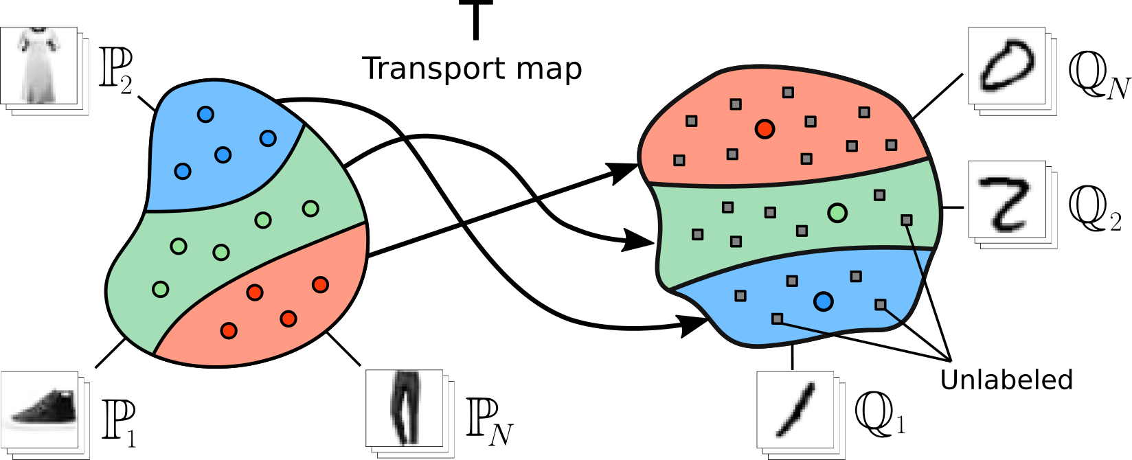
Figure 1: Dataset transfer problem. Input $\mathbb{P}=\sum_{n}\alpha_{n}\mathbb{P}_{n}$, target $\mathbb{Q}=\sum_{n}\beta_{n}\mathbb{Q}_{n}$ distributions are mixtures of $N$ classes. The task is to learn a transport map $T$ preserving the class. The learner has the access to labeled input data $\sim\mathbb{P}$ and only partially labeled target data $\sim\mathbb{Q}$.

Optimal transport (OT) is a powerful framework to solve mass-moving problems for data distributions which finds many applications in machine learning and computer vision (Bonneel & Digne, 2023). Most existing methods to compute OT plans are designed for discrete distributions (Flamary et al., 2021; Peyré et al., 2019; Cuturi, 2013). These methods have good flexibility: they allow to control the properties of the plan via choosing the cost function. However, discrete methods find an optimal matching between two given (train) sets which does not generalize to new (test) data points. This limits the applications of discrete OT plan methods to scenarios when one needs to generate new data, e.g., image-to-image transfer (Zhu et al., 2017).

Recent works (Rout et al., 2022; Korotin et al., 2023b; 2021b; Fan et al., 2021a; Daniels et al., 2021) propose continuous methods to compute OT plans. Thanks to employing neural networks to parameterize OT solutions, the learned transport plan can be used directly as the generative model in data synthesis (Rout et al., 2022) and unpaired learning (Korotin et al., 2023b; Rout et al., 2022; Daniels et al., 2021; Gazdieva et al., 2022).

Existing continuous OT methods mostly focus on classic cost functions such as $\ell^{2}$ (Korotin et al., 2021b; 2023b; Fan et al., 2021a; Gazdieva et al., 2022) which estimate the closeness of input and output points. However, choosing such costs for problems where a specific optimality of the mapping is required may be challenging. For example, when one needs to preserve the object class during the transport (Figure 1), common $\ell^{2}$ cost may be suboptimal (Su et al., 2022, Appendix C), (Daniels et al., 2021, Figure 3). This limitation could be fixed by considering general cost functionals (Paty & Cuturi, 2020) which may take into account additional information, e.g., class labels.

Despite the large popularity of OT, the approach for continuous OT with general cost functionals (general OT) is still missing. We address this limitation. The main contributions of our paper are:

1. We show that the general OT problem (1) can be reformulated as a saddle point optimization problem (3.1), which allows to implicitly recover the OT plan (3.2) in the continuous setting. The problem can be solved with neural networks and stochastic gradient methods (Algorithm 2).

2. We provide the error analysis of solving the proposed saddle point optimization problem via the duality gaps, i.e., errors for solving inner and outer optimization problems (3.3).

3. We construct and test an example of a general cost functional for mapping data distributions with the preservation of the class-wise structure ( 1, Algorithm 1, 5).

From the theoretical perspective, our max-min reformulation is generic and subsumes previously known reformulations for classic (Fan et al., 2023; Rout et al., 2022) and weak (Korotin et al., 2021b) OT. Furthermore, existing error analysis works exclusively with the classic OT and operate only under certain restrictive assumptions such as the the convexity of the dual potential. Satisfying these assumptions in practice leads to a severe performance drop (Korotin et al., 2021c, Figure 5a). In contrast, our error analysis is free from assumptions on the dual variable and, besides general OT, it is applicable to weak OT for which there is currently no existing error analysis.

From the practical perspective, we apply our method to the dataset transfer problem (Figure 1), previously not solved using continuous optimal transport. This problem arises when it is necessary to repurpose fixed or black-box models to classify previously unseen partially labelled target datasets with high accuracy by mapping the data into the dataset on which the classifier was trained. The dataset transfer problem was previously considered in related OT literature (Alvarez-Melis & Fusi, 2021). Our method achieves notable improvements in accuracy over existing algorithms.

1 Background and Notations

In this section, we provide key concepts of the optimal transport theory. Throughout the paper, we consider compact $\mathcal{X}=\mathcal{Y}\subset\mathbb{R}^{D}$ and $\mathbb{P},\mathbb{Q}\in\mathcal{P}(\mathcal{X}),\mathcal{P}(\mathcal{Y})$.

Notations. The notation of our paper is based on that of (Paty & Cuturi, 2020; Korotin et al., 2023b). For a compact Hausdorf space $\mathcal{S}$, we use $\mathcal{P}(\mathcal{S})$ to denote the set of Borel probability distributions on $\mathcal{S}$. We denote the space of continuous $\mathbb{R}$-valued functions on $\mathcal{S}$ endowed with the supremum norm by $\mathcal{C}(\mathcal{S})$. Its dual space is the space $\mathcal{M}(\mathcal{S})\supset\mathcal{P}(\mathcal{S})$ of finite signed Borel measures over $\mathcal{S}$. For a functional $\mathcal{F}\!:\mathcal{M}(\mathcal{S})\!\rightarrow\!\mathbb{R}\cup\{\infty\}$, we use $\mathcal{F}^{*}(h)\stackrel{{\scriptstyle def}}{{=}}\!\!\sup_{\pi\in\mathcal{M}(\mathcal{S})}\!\left[\int_{\mathcal{S}}h(s)d\pi(s)\!-\!\mathcal{F}(\pi)\right]$ to denote its convex conjugate ${\mathcal{F}^{*}:C(\mathcal{S})\!\rightarrow\!\mathbb{R}\cup\{\infty\}}$. Let $\mathcal{X},\mathcal{Y}$ be compact Hausdorf spaces and $\mathbb{P}\in\mathcal{P}(\mathcal{X})$, $\mathbb{Q}\in\mathcal{P}(\mathcal{Y})$. We use $\Pi(\mathbb{P})\subset\mathcal{P}(\mathcal{X}\times\mathcal{Y})$ to denote the subset of probability distributions on $\mathcal{X}\times\mathcal{Y}$, which projection onto the first marginal is $\mathbb{P}$. We use $\Pi(\mathbb{P},\mathbb{Q})\subset\Pi(\mathbb{P})$ to denote the subset of probability distributions (transport plans) on $\mathcal{X}\times\mathcal{Y}$ with marginals $\mathbb{P},\mathbb{Q}$. For $u,v\in\mathcal{C}(\mathcal{X}),\mathcal{C}(\mathcal{Y})$ we write $u\oplus v\in\mathcal{C}(\mathcal{X}\times\mathcal{Y})$ to denote the function $u\oplus v:(x,y)\mapsto u(x)+v(y)$. For a functional $\mathcal{F}:\mathcal{M}(\mathcal{X}\times\mathcal{Y})\rightarrow\mathbb{R}$ we say that it is separably *-increasing if for all functions $u,v\in\mathcal{C}(\mathcal{X}),\mathcal{C}(\mathcal{Y})$ and any function $c\in\mathcal{C}(\mathcal{X}\times\mathcal{Y})$ from $u\oplus v\leq c\text{ (point-wise)}$ it follows $\mathcal{F}^{*}(u\oplus v)\leq\mathcal{F}^{*}(c).$ For a measurable map $T:\mathcal{X}\times\mathcal{Z}\rightarrow\mathcal{Y}$, we denote the associated push-forward operator by $T_{\#}$.

Classic and weak OT. For a cost function $c\in\mathcal{C}(\mathcal{X}\times\mathcal{Y})$, the OT cost between $\mathbb{P},\mathbb{Q}$ is

$$\text{Cost}(\mathbb{P},\mathbb{Q})\stackrel{{\scriptstyle\text{def}}}{{=}}\inf_{\pi\in\Pi(\mathbb{P},\mathbb{Q})}\int_{\mathcal{X}\times\mathcal{Y}}c(x,y)d\pi(x,y),$$ (1)

see (Villani, 2008, 1). We call (1) the classic OT. Problem (1) admits a minimizer $\pi^{*}\in\Pi(\mathbb{P},\mathbb{Q})$, which is called an OT plan (Santambrogio, 2015, Theorem 1.4). It may be not unique (Peyré et al., 2019, Remark 2.3). Intuitively, the cost function $c(x,y)$ measures how hard it is to move a mass piece between points $x\in\mathcal{X}$ and $y\in\mathcal{Y}$. That is, $\pi^{*}$ shows how to optimally distribute the mass of $\mathbb{P}$ to $\mathbb{Q}$, i.e., with minimal effort. For cost functions $c(x,y)=\|x-y\|_{2}$ and $c(x,y)=\frac{1}{2}\|x-y\|_{2}^{2}$, the OT cost (1) is called the Wasserstein-1 ($\mathbb{W}_{1}$) and the (square of) Wasserstein-2 ($\mathbb{W}_{2}$) distance, respectively, see (Villani, 2008, 1) or (Santambrogio, 2015, 1, 2).

Recently, classic OT obtained the weak OT extension (Gozlan et al., 2017; Backhoff-Veraguas et al., 2019). Consider ${C:\mathcal{X}\times\mathcal{P}(\mathcal{Y})\rightarrow\mathbb{R}}$, i.e., a weak cost function whose inputs are a point $x\in\mathcal{X}$ and a distribution of $y\in\mathcal{Y}$. The weak OT cost is

$$\text{Cost}(\mathbb{P},\mathbb{Q})\stackrel{{\scriptstyle\text{def}}}{{=}}\inf_{\pi\in\Pi(\mathbb{P},\mathbb{Q})}\int_{\mathcal{X}}C\big{(}x,\pi(\cdot|x)\big{)}d\pi(x),$$ (2)

where $\pi(\cdot|x)$ denotes the conditional distribution. Weak formulation (2) is reduced to classic formulation (1) when $C(x,\mu)=\int_{\mathcal{Y}}c(x,y)d\mu(y)$. Another example of a weak cost function is the $\gamma$-weak quadratic cost $C\big{(}x,\mu\big{)}=\int_{\mathcal{Y}}\frac{1}{2}\|x-y\|_{2}^{2}d\mu(y)-\frac{\gamma}{2}\text{Var}(\mu),$ where $\gamma\geq 0$ and $\text{Var}(\mu)$ is the variance of $\mu$, see (Korotin et al., 2023b, Eq. 5), (Alibert et al., 2019, 5.2), (Gozlan & Juillet, 2020, 5.2) for details. For this cost, we denote the optimal value of (2) by $\mathcal{W}_{2,\gamma}^{2}$ and call it $\gamma$-weak Wasserstein-2.

Regularized and general OT. The expression inside (1) is a linear functional. It is common to add a lower semi-continuous convex regularizer $\mathcal{R}:\mathcal{M}(\mathcal{X}\times\mathcal{Y})\rightarrow\mathbb{R}\cup\{\infty\}$ with weight $\gamma>0$:

$$\text{Cost}(\mathbb{P},\mathbb{Q})\stackrel{{\scriptstyle\text{def}}}{{=}}\inf_{\pi\in\Pi(\mathbb{P},\mathbb{Q})}\left\{\int_{\mathcal{X}\times\mathcal{Y}}c(x,y)d\pi(x,y)+\gamma\mathcal{R}(\pi)\right\}.$$ (3)

Regularized OT formulation (3) typically provides several advantages over original formulation (1). For example, if $\mathcal{R}(\pi)$ is strictly convex, the expression inside (3) is a strictly convex functional in $\pi$ and yields the unique OT plan $\pi^{*}$. Besides, regularized OT typically has better sample complexity (Genevay, 2019; Mena & Niles-Weed, 2019; Genevay et al., 2019). Common regularizers are the entropic (Cuturi, 2013), quadratic (Essid & Solomon, 2018), lasso (Courty et al., 2016), etc.

To consider a general OT formulation let $\mathcal{F}:\mathcal{M}(\mathcal{X}\times\mathcal{Y})\rightarrow\mathbb{R}\cup\{+\infty\}$ be a convex lower semi-continuous functional. Assume that there exists $\pi\in\Pi(\mathbb{P},\mathbb{Q})$ for which $\mathcal{F}(\pi)<\infty$. Let

$$\text{Cost}(\mathbb{P},\mathbb{Q})\stackrel{{\scriptstyle\text{def}}}{{=}}\inf_{\pi\in\Pi(\mathbb{P},\mathbb{Q})}\mathcal{F}(\pi).$$ (4)

This problem is a generalization of classic OT (1), weak OT (2), and regularized OT (3). Following (Paty & Cuturi, 2020), we call problem (4) a general OT problem. One may note that regularized OT (3) represents a similar problem: it is enough to put $c(x,y)\equiv 0$, $\gamma=1$ and $\mathcal{R}(\pi)=\mathcal{F}(\pi)$ to obtain (4) from (3), i.e., regularized (3) and general OT (4) can be viewed as equivalent formulations.

With mild assumptions on $\mathcal{F}$, general OT problem (4) admits a minimizer $\pi^{*}$ (Paty & Cuturi, 2020, Lemma 1). If $\mathcal{F}$ is separately *-increasing, the dual problem is given by

$$\text{Cost}(\mathbb{P},\mathbb{Q})=\sup_{u,v}\left[\int_{\mathcal{X}}u(x)d\mathbb{P}(x)+\int_{\mathcal{Y}}v(y)d\mathbb{Q}(y)-\mathcal{F}^{*}(u\oplus v)\right],$$ (5)

where optimization is performed over $u,v\in\mathcal{C}(\mathcal{X}),\mathcal{C}(\mathcal{Y})$ which are called potentials (Paty & Cuturi, 2020, Theorem 2). The popular regularized functionals (3) are indeed separately *-increasing, including the OT regularized with entropy (Paty & Cuturi, 2020, Example 7) or $L^{p}$ (Paty & Cuturi, 2020, Example 8). That is, formulation (5) subsumes many known duality formulas for OT.

2 Related Work: Discrete and Continuous OT solvers

Solving OT problems usually implies either finding an OT plan $\pi^{*}$ or dual potentials $u^{*},v^{*}$. Existing computational OT methods can be roughly split into two groups: discrete and continuous.

Discrete OT considers discrete distributions $\widehat{\mathbb{P}}_{N}=\sum_{n=1}^{N}p_{n}\delta_{x_{n}}$ and $\widehat{\mathbb{Q}}_{N}=\sum_{m=1}^{M}q_{m}\delta_{y_{m}}$ and aims to find the OT plan (1), (2), (4), (3) directly between $\mathbb{P}=\widehat{\mathbb{P}}_{N}$ and $\mathbb{Q}=\widehat{\mathbb{Q}}_{M}$. In this case, the OT plan $\pi^{*}$ can be represented as a doubly stochastic $N\times M$ matrix. For a survey of computational methods for discrete OT, we refer to (Peyré et al., 2019). In short, one of the most popular is the Sinkhorn algorithm (Cuturi, 2013) which is designed to solve formulation (3) with the entropic regularization.

General discrete OT is extensively studied (Nash, 2000; Courty et al., 2016; Flamary et al., 2021; Ferradans et al., 2014; Rakotomamonjy et al., 2015); these methods are often employed in domain adaptation problems (Courty et al., 2016). Additionally, the available labels can be used to reconstruct the classic cost function, to capture the underlying data structure (Courty et al., 2016; Stuart & Wolfram, 2020; Liu et al., 2020; Li et al., 2019).

The major drawback of discrete OT methods is that they only perform a (stochastic) matching between the given empirical samples and usually do not provide out-of-sample estimates. This limits their application to real-world scenarios where new (test) samples frequently appear. Recent works (Hütter & Rigollet, 2021; Pooladian & Niles-Weed, 2021; Manole et al., 2021; Deb et al., 2021) consider the OT problem with the quadratic cost and develop out-of-sample estimators by wavelet/kernel-based plugin estimators or by the barycentric projection of the discrete entropic OT plan. In spite of tractable theoretical properties, the performance of such methods in high dimensions is questionable.

Continuous OT usually considers $p_{n}=\frac{1}{N}$ and $q_{n}=\frac{1}{M}$ and assumes that the given discrete distributions $\widehat{\mathbb{P}}_{N}=\frac{1}{N}\sum_{n=1}^{N}\delta_{x_{n}},\widehat{\mathbb{Q}}_{M}=\frac{1}{M}\sum_{m=1}^{M}\delta_{y_{m}}$ are the empirical counterparts of the underlying distributions $\mathbb{P}$, $\mathbb{Q}$. That is, the goal of continuous OT is to recover the OT plan between $\mathbb{P},\mathbb{Q}$ which are accessible only by their (finite) empirical samples $\{x_{1},x_{2},\dots,x_{N}\}\sim\mathbb{P}$ and $\{y_{1},y_{2},\dots,y_{M}\}\sim\mathbb{Q}$. In this case, to represent the plan one has to employ parametric approximations of the OT plan $\pi^{*}$ or dual potentials $u^{*},v^{*}$ which, in turn, provide straightforward out-of-sample estimates.

A notable development is the use of neural networks to compute OT maps for solving weak (2) and classic (1) functionals (Korotin et al., 2023b; 2022a; 2021b; Rout et al., 2022; Fan et al., 2021a; Henry-Labordere, 2019). Previous OT methods were based on formulations restricted to convex potentials (Makkuva et al., 2020; Korotin et al., 2021a; c; Mokrov et al., 2021; Fan et al., 2023; Bunne et al., 2021; Alvarez-Melis et al., 2021), and used Input Convex Neural Networks (Amos et al., 2017, ICNN) to approximate them, which limited the application of OT in large-scale tasks (Korotin et al., 2021b; Fan et al., 2021b; Korotin et al., 2022a). In (Genevay et al., 2016; Seguy et al., 2017; Daniels et al., 2021; Fan et al., 2021b), the authors propose methods for $f$-divergence regularized functionals (3). In particular, (Genevay et al., 2016; Seguy et al., 2017) recover biased plans, which is a notable issue in high dimensions (Korotin et al., 2021b, 4.2). The method in (Daniels et al., 2021) is computationally heavy due to using Langevin dynamics. Additionally, many approaches in generative learning use OT cost as the loss function to update generative models, such as WGANs (Arjovsky & Bottou, 2017; Petzka et al., 2017; Liu et al., 2019), see (Korotin et al., 2022b) for a survey. These are not related to our work as they do not compute OT plans or maps.

Our work vs. prior works. While the discrete version of the general OT problem (4) is well studied in the literature, its continuous counterpart is not yet analyzed. The above-mentioned continuous methods focus on special cases, e.g., on weak and classic cost functionals (rather than general OT). Such functionals are suitable for the tasks of unpaired image-to-image style translation (Zhu et al., 2017, Figures 1,2). However, they typically do not take into account the class-wise structure of data or available side information, e.g., the class labels. As a result, such methods are hardly applicable to certain tasks such as the dataset transfer where the preservation of the class-wise structure is required. Therefore, in our work, we fill this gap by proposing the algorithm to solve the (continuous) general OT problem (3), provide error bounds (3.3). As an illustration, we construct an example general OT cost functional which can take into account the available task-specific information (1).

3 Maximin Reformulation of the General OT

In this section, we derive a saddle point formulation for the general OT problem (4) which we later solve with neural networks. All the proofs of the statements are given in Appendix A.

3.1 Maximin Reformulation of the Dual Problem

In this subsection, we derive the dual form, which is an alternative to (5) and can be used to get the OT plan $\pi^{*}$. Our two following theorems constitute the main theoretical idea of our approach.

Theorem 1 (Maximin reformulation of the dual problem).

For *-separately increasing convex and lower semi-continuous functional $\mathcal{F}:\mathcal{M}(\mathcal{X}\!\times\!\mathcal{Y})\!\rightarrow\!\mathbb{R}\!\cup\!\{+\infty\}$ it holds

$$\mbox{Cost}(\mathbb{P},\mathbb{Q})\!=\!\sup_{v}\inf_{\pi\in\Pi(\mathbb{P})}\mathcal{L}(v,\pi)=\sup_{v}\inf_{\pi\in\Pi(\mathbb{P})}\left\{\big{[}\mathcal{F}(\pi)-\int_{\mathcal{Y}}v(y)d\pi(y)]\!+\!\int_{\mathcal{Y}}v(y)d\mathbb{Q}(y)\right\},$$ (6)

where the $\sup$ is taken over $v\!\in\!\mathcal{C}(\mathcal{Y})$ and $\pi(y)$ is the marginal distribution over $y$ of the plan $\pi$.

From (6) we also see that it is enough to consider values of $\mathcal{F}$ in $\pi\in\Pi(\mathbb{P})\subset\mathcal{M}(\mathcal{X}\times\mathcal{Y})$. For convention, in further derivations we always consider $\mathcal{F}(\pi)=+\infty$ for $\pi\in\mathcal{M}(\mathcal{X}\times\mathcal{Y})\setminus\Pi(\mathbb{P})$.

Theorem 2 (Optimal saddle points provide optimal plans).

Let $v^{*}\!\in\!\operatorname*{arg\,sup}_{v}\inf_{\pi\in\Pi(\mathbb{P})}\!\mathcal{L}(v,\pi)$ be any optimal potential. Then for every OT plan $\pi^{*}\in\Pi(\mathbb{P},\mathbb{Q})$ it holds:

$$\pi^{*}\in\operatorname*{arg\,inf}_{\pi\in\Pi(\mathbb{P})}\mathcal{L}(v^{*},\pi).$$ (7)

If $\mathcal{F}$ is strictly convex in $\pi\in\Pi(\mathbb{P})$, then $\mathcal{L}(v^{*},\pi)$ is strictly convex as a functional of $\pi$. Consequently, it has a unique minimizer. As a result, expression (7) is an equality. We have the following corollary.

Corollary 1 (Every optimal saddle point provides the OT plan).

Assume additionally that $\mathcal{F}$ is strictly convex. Then the unique OT plan satisfies $\pi^{*}=\operatorname*{arg\,inf}_{\pi\in\Pi(\mathbb{P})}\mathcal{L}(v^{*},\pi)$.

Using our results above, one may solve (6) and obtain the OT plan $\pi^{*}$ from the solution $(v^{*},\pi^{*})$ of the saddle point problem (6). The challenging part is to optimize over the distributions $\pi\in\Pi(\mathbb{P})$.

3.2 General OT Maximin Reformulation via Stochastic Maps

To make optimization over probability distributions $\pi\in\Pi(\mathbb{P})$ practically feasible, we reformulate it as the optimization over functions $T$ which generate them. Inspired by (Korotin et al., 2023b, 4.1), we introduce a latent space $\mathcal{Z}=\mathbb{R}^{Z}$ and an atomless distribution $\mathbb{S}\in\mathcal{P}(\mathcal{Z})$ on it, e.g., $\mathbb{S}=\mathcal{N}(0,I_{Z})$. For every $\pi\in\mathcal{P}(\mathcal{X}\times\mathcal{Y})$, there exists a measurable function $T=T_{\pi}:\mathcal{X}\times\mathcal{Z}\rightarrow\mathcal{Y}$ which implicitly represents it. Such $T_{\pi}$ satisfies $T_{\pi}(x,\cdot)\sharp\mathbb{S}=\pi(\cdot|x)$ for all $x\in\mathcal{X}$. That is, given $x\in\mathcal{X}$ and a random latent vector $z\sim\mathbb{S}$, the function $T$ produces sample $T_{\pi}(x,z)\sim\pi(y|x)$. In particular, if $x\sim\mathbb{P}$, the random vector $[x,T_{\pi}(x,z)]$ is distributed as $\pi$. Thus, every $\pi\in\Pi(\mathbb{P})$ can be implicitly represented as a function $T_{\pi}:\mathcal{X}\times\mathcal{Z}\rightarrow\mathcal{Y}$. Note that there might exist several suitable $T_{\pi}$.

Every measurable function $T:\mathcal{X}\times\mathcal{Z}\rightarrow\mathcal{Y}$ is an implicit representation of the distribution $\pi_{T}$ which is the joint distribution of a random vector $[x,T(x,z)]$ with $x\sim\mathbb{P},z\sim\mathbb{S}$. Consequently, the optimization over $\pi\in\Pi(\mathbb{P})$ is equivalent to the optimization over measurable functions $T:\mathcal{X}\times\mathcal{Z}\rightarrow\mathcal{Y}$. From our Theorem 1, we have the following corollary.

Corollary 2.

For *-separately increasing, lower semi-continuous and convex $\mathcal{F}$ it holds

$$\mbox{Cost}(\mathbb{P},\mathbb{Q})\!=\!\sup_{v}\inf_{T}\widetilde{\mathcal{L}}(v,T)\!=\sup_{v}\inf_{T}\bigg{\{}\!\widetilde{\mathcal{F}}(T)-\int_{\mathcal{X}\times\mathcal{Z}}\!v\big{(}T(x,z)\big{)}d\mathbb{P}(x)d\mathbb{S}(z)\!+\!\int_{\mathcal{Y}}\!v(y)d\mathbb{Q}(y)\!\bigg{\}},$$

where the $\sup$ is taken over potentials $v\in\mathcal{C}(\mathcal{Y})$ and $\inf$ – over measurable functions $T:\mathcal{X}\times\mathcal{Z}\rightarrow\mathcal{Y}$. Here we identify $\widetilde{\mathcal{F}}(T)\stackrel{{\scriptstyle def}}{{=}}\mathcal{F}(\pi_{T})$ and $\widetilde{\mathcal{L}}(v,T)\stackrel{{\scriptstyle def}}{{=}}\mathcal{L}(v,\pi_{T})$.

We say that $T^{*}$ is a stochastic OT map if it represents some OT plan $\pi^{*}$, i.e., $T^{*}(x,\cdot)\sharp\mathbb{S}=\pi^{*}(\cdot|x)$ holds $\mathbb{P}$-almost surely for all $x\!\in\!\mathcal{X}$. From Theorem 7 and Corollary 1, we obtain the following result.

Corollary 3 (Optimal saddle points provide stochastic OT maps).

Let ${v^{*}\!\in\!\operatorname*{arg\,sup}_{v}\inf_{T}\!\widetilde{\mathcal{L}}(v,T)}$ be any optimal potential. Then for every stochastic OT map $T^{*}$ it holds:

$$T^{*}\in\operatorname*{arg\,inf}_{T}\widetilde{\mathcal{L}}(v^{*},T).$$ (8)

If $\mathcal{F}$ is strictly convex in $\pi$, we have $T^{*}\in\operatorname*{arg\,inf}_{T}\widetilde{\mathcal{L}}(v^{*},T)\Leftrightarrow T^{*}$ is a stochastic OT map.

From our results it follows that by solving (2) and obtaining an optimal saddle point $(v^{*},T^{*})$, one gets a stochastic OT map $T^{*}$. To ensure that all the solutions are OT maps, one may consider adding strictly convex regularizers to $\mathcal{F}$ with a small weight, e.g., conditional interaction energy, see Appendices D and D.1 which is also known as the conditional kernel variance (Korotin et al., 2023a).

Overall, problem (2) replaces the optimization over distributions $\pi\in\Pi(\mathbb{P})$ in (6) with the optimization over stochastic maps $T$, making it practically feasible. After our reformulation, every term in (2) can be estimated with Monte Carlo by using random empirical samples from $\mathbb{P},\mathbb{Q}$, allowing us to approach the general OT problem (4) in the continuous setting (2). To solve the problem (2) in practice, one may use neural networks $T_{\theta}:\mathbb{R}^{D}\times\mathbb{R}^{S}\rightarrow\mathbb{R}^{D}$ and $v_{\omega}:\mathbb{R}^{D}\rightarrow\mathbb{R}$ to parametrize $T$ and $v$, respectively. To train them, one may employ stochastic gradient ascent-descent (SGAD) by using random batches from $\mathbb{P},\mathbb{Q},\mathbb{S}$. We summarize the optimization procedure for general cost functionals $\mathcal{F}$ in Algorithm 2 of Appendix B. In the main text below (1), we focus on the special case of the class-guided functional $\mathcal{F}_{\text{G}}$, which is targeted to be used in the dataset transfer task (Figure 1).

Relation to prior works. Maximin reformulations analogous to our (2) appear in the continuous OT literature (Korotin et al., 2021c; 2023b; Rout et al., 2022; Fan et al., 2021a) yet they are designed only for classic (1) and weak (2) OT. Our formulation is generic and automatically subsumes all of them. Importantly, it allows using general cost functionals $\mathcal{F}$ which, e.g., may easily take into account side information such as the class labels, see 1.

3.3 Error Bounds for Approximate Solutions for General OT

For a pair ($\hat{v},\hat{\pi}$) approximately solving (6), it is natural to ask how close is $\hat{\pi}$ to the OT plan $\pi^{*}$. Based on the duality gaps, i.e., errors for solving outer and inner optimization problems with $(\hat{v},\hat{\pi})$ in (6), we give an upper bound on the difference between $\hat{\pi}$ and $\pi^{*}$. Our analysis holds for functionals $\mathcal{F}$ which are strongly convex in some metric $\rho(\cdot,\cdot)$, see Definition 1 in Appendix A. Recall that the strong convexity of $\mathcal{F}$ also implies the strict convexity, i.e., the OT plan $\pi^{*}$ is unique.

Theorem 3 (Error analysis via duality gaps).

Let $\mathcal{F}:\mathcal{M}(\mathcal{X}\times\mathcal{Y})\rightarrow\mathbb{R}\cup\{+\infty\}$ be a convex cost functional. Let $\rho(\cdot,\cdot)$ be a metric on $\Pi(\mathbb{P})\subset\mathcal{M}(\mathcal{X}\times\mathcal{Y})$. Assume that $\mathcal{F}$ is $\beta$-strongly convex in $\rho$ on $\Pi(\mathbb{P})$. Consider the duality gaps for an approximate solution $(\hat{v},\hat{\pi})\in\mathcal{C}(\mathcal{Y})\times\Pi(\mathbb{P})$ of (6):

$$\vspace{1.9mm}\epsilon_{1}(\hat{v},\hat{\pi})\!\stackrel{{\scriptstyle\mbox{def}}}{{=}}\!\mathcal{L}(\hat{v},\hat{\pi})-\!\!\!\inf\limits_{\pi\in\Pi(\mathbb{P})}\!\!\mathcal{L}(\hat{v},\pi),\!\!\!$$ (9)

$$\vspace{2mm}\epsilon_{2}(\hat{v})\stackrel{{\scriptstyle\mbox{def}}}{{=}}\sup\limits_{v}\!\!\inf\limits_{\pi\in\Pi(\mathbb{P})}\!\!\mathcal{L}(v,\pi)-\!\!\!\!\!\inf\limits_{\pi\in\Pi(\mathbb{P})}\!\!\mathcal{L}(\hat{v},\pi),\!\!\!$$ (10)

which are the errors of solving the outer $\sup_{v}$ and inner $\inf_{\pi}$ problems in (6), respectively. Then for OT plan $\pi^{*}$ in (4) between $\mathbb{P}$ and $\mathbb{Q}$ the following inequality holds

$$\rho(\hat{\pi},\pi^{*})\leq\sqrt{\frac{2}{\beta}}\left(\sqrt{\epsilon_{1}(\hat{v},\hat{\pi})}+\sqrt{\epsilon_{2}(\hat{v})}\right),$$ (11)

i.e., the sum of the roots of duality gaps upper bounds the error of the plan $\hat{\pi}$ w.r.t. $\pi^{*}$ in $\rho(\cdot,\cdot)$.

The significance of our Theorem 3 is manifested when moving from theoretical objectives (5), (6) to its numerical counterparts. In practice, the dual potential $v$ in (6) is parameterized by NNs (a subset of continuous functions) and may not reach the optimizer $v^{*}$. Our duality gap analysis shows that we can still find a good approximation of the OT plan. It suffices to find a pair $(\hat{v},\hat{\pi})$ that achieves nearly optimal objective values in the inner $\inf_{\pi}$ and outer $\sup_{v}$ problems of (6). In such a pair, $\hat{\pi}$ is close to the OT plan $\pi^{*}$. To apply our duality gap analysis the strong convexity of $\mathcal{F}$ is required. We give an example of a strongly convex regularizer and a general recipe for using it in Appendix D. In turn, Appendix D.1 demonstrates the application of this regularization technique in practice.

Relation to prior works. The authors of (Fan et al., 2021a), (Rout et al., 2022), (Makkuva et al., 2020) carried out error analysis via duality gaps resembling our Theorem 3. Their error analysis works only for classic OT (1) and requires the potential $\hat{v}$ to satisfy certain convexity properties. Our error analysis is free from assumptions on $\hat{v}$ and works for general OT (4) with strongly convex $\mathcal{F}$.

4 Learning with the Class-Guided Cost Functional

Input : Distributions $\mathbb{P}=\sum_{n}\alpha_{n}\mathbb{P}_{n}$, $\mathbb{Q}=\sum_{n}\beta_{n}\mathbb{Q}_{n}$, $\mathbb{S}$ accessible by samples (unlabeled); weights $\alpha_{n}$ are known and samples from each $\mathbb{P}_{n},\mathbb{Q}_{n}$ are accessible (labeled);

mapping network $T_{\theta}:\mathbb{R}^{P}\times\mathbb{R}^{S}\rightarrow\mathbb{R}^{Q}$; potential network $v_{\omega}:\mathbb{R}^{Q}\rightarrow\mathbb{R}$;

number of inner iterations $K_{T}$;

Output : Learned stochastic OT map $T_{\theta}$ representing an OT plan between distributions $\mathbb{P},\mathbb{Q}$;

repeat

     Sample (unlabeled) batches $Y\sim\mathbb{Q}$, $X\sim\mathbb{P}$ and for each $x\in X$ sample batch $Z[x]\sim\mathbb{S}$;

     ${\mathcal{L}_{v}\leftarrow\sum\limits_{x\in X}\sum\limits_{z\in Z[x]}\frac{v_{\omega}(T_{\theta}(x,z))}{|X|\cdot|Z[x]|}-\sum\limits_{y\in Y}\frac{v_{\omega}(y)}{|Y|}}$;

     Update $\omega$ by using $\frac{\partial\mathcal{L}_{v}}{\partial\omega}$;

     for $k_{T}=1,2,\dots,K_{T}$ do

         Pick $n\in\{1,2,\dots,N\}$ at random with probabilities $(\alpha_{1},\dots,\alpha_{N})$;

         Sample (labeled) batches $X_{n}\sim\mathbb{P}_{n}$, $Y_{n}\sim\mathbb{Q}_{n}$; for each $x\in X$ sample batch $Z_{n}[x]\sim\mathbb{S}$;

        

        $\mathcal{L}_{T}\leftarrow\widehat{\Delta\mathcal{E}^{2}}\big{(}X_{n},T(X_{n},Z_{n}),Y_{n}\big{)}-\sum\limits_{x\in X_{n}}\sum\limits_{z\in Z_{n}[x]}\frac{v_{\omega}(T_{\theta}(x,z))}{|X_{n}|\cdot|Z_{n}[x]|}$;

         Update $\theta$ by using $\frac{\partial\mathcal{L}_{T}}{\partial\theta}$;

        

    

until not converged;

Algorithm 1 Neural optimal transport with the class-guided cost functional $\widetilde{\mathcal{F}}_{\text{G}}$.

In this section, we show that general cost functionals (4) are useful, for example, for the class-guided dataset transfer (Figure 1). To begin with, we theoretically formalize the problem setup.

Let each input $\mathbb{P}$ and output $\mathbb{Q}$ distributions be a mixture of $N$ distributions (classes) $\{\mathbb{P}_{n}\}_{n=1}^{N}$ and $\{\mathbb{Q}_{n}\}_{n=1}^{N}$, respectively. That is $\mathbb{P}=\sum_{n=1}^{N}\alpha_{n}\mathbb{P}_{n}$ and $\mathbb{Q}=\sum_{n=1}^{N}\beta_{n}\mathbb{Q}_{n}$ where $\alpha_{n},\beta_{n}\geq 0$ are the respective weights (class prior probabilities) satisfying $\sum_{n=1}^{N}\alpha_{n}=1$ and $\sum_{n=1}^{N}\beta_{n}=1$. In this general setup, we aim to find the transport plan $\pi(x,y)\in\Pi(\mathbb{P},\mathbb{Q})$ for which the classes of $x\in\mathcal{X}$ and $y\in\mathcal{Y}$ are the same for as many pairs $(x,y)\sim\pi$ as possible. That is, its respective stochastic map $T$ should map each component $\mathbb{P}_{n}$ (class) of $\mathbb{P}$ to the respective component $\mathbb{Q}_{n}$ (class) of $\mathbb{Q}$.

The task above is related to domain adaptation or transfer learning problems. It does not always have a solution with each $\mathbb{P}_{n}$ exactly mapped to $\mathbb{Q}_{n}$ due to possible prior/posterior shift (Kouw & Loog, 2018). We aim to find a stochastic map $T$ between $\mathbb{P}$ and $\mathbb{Q}$ satisfying $T_{\sharp}(\mathbb{P}_{n}\!\times\!\mathbb{S})\approx\mathbb{Q}_{n}$ for all $n=1,\dots,N$. To solve the above-discussed problem, we propose the following functional:

$$\mathcal{F}_{\text{G}}(\pi)=\widetilde{\mathcal{F}}_{\text{G}}(T_{\pi})\stackrel{{\scriptstyle def}}{{=}}\sum_{n=1}^{N}\alpha_{n}\mathcal{E}^{2}\big{(}T_{\pi}\sharp(\mathbb{P}_{n}\times\!\mathbb{S}),\mathbb{Q}_{n}\big{)},$$ (12)

where $\mathcal{E}$ denotes the energy distance (13). For two distributions $\mathbb{Q},\mathbb{Q}^{\prime}\in\mathcal{P}(\mathcal{Y})$ with $\mathcal{Y}\subset\mathbb{R}^{D}$, the (square of) energy distance $\mathcal{E}$ (Rizzo & Székely, 2016) between them is:

$$\mathcal{E}^{2}(\mathbb{Q},\mathbb{Q}^{\prime})=\mathbb{E}\|Y_{1}-Y_{2}\|_{2}-\frac{1}{2}\mathbb{E}\|Y_{1}-Y^{\prime}_{1}\|_{2}-\frac{1}{2}\mathbb{E}\|Y_{2}-Y^{\prime}_{2}\|_{2},$$ (13)

where $Y_{1}\sim\mathbb{Q},Y_{1}^{\prime}\sim\mathbb{Q},Y_{2}\sim\mathbb{Q}^{\prime},Y_{2}^{\prime}\sim\mathbb{Q}^{\prime}$ are independent random vectors. Energy distance (13) is a particular case of the Maximum Mean Discrepancy (Sejdinovic et al., 2013). It equals zero only when $\mathbb{Q}_{1}=\mathbb{Q}_{2}$. Hence, our functional (12) is non-negative and attains zero value when the components of $\mathbb{P}$ are correctly mapped to the respective components of $\mathbb{Q}$ (if this is possible).

Theorem 4 (Properties of the class-guided cost functional $\mathcal{F}_{\text{G}}$).

Functional $\mathcal{F}_{\text{G}}(\pi)$ is convex in $\pi\in\Pi(\mathbb{P})$, lower semi-continuous and $*$-separably increasing.

In practice, each of the terms $\mathcal{E}^{2}\big{(}T_{\pi}\sharp(\mathbb{P}_{n}\times\!\mathbb{S}),\mathbb{Q}_{n}\big{)}$ in (12) admits estimation from samples from $\pi$.

Proposition 1 (Estimator for $\mathcal{E}^{2}$).

Let $X_{n}\sim\mathbb{P}_{n}$ be a batch of $K_{X}$ samples from class $n$. For each $x\in X_{n}$ let $Z_{n}[x]\sim\mathbb{S}$ be a latent batch of size $K_{Z}$. Consider a batch $Y_{n}\sim\mathbb{Q}_{n}$ of size $K_{Y}$. Then

$$\widehat{\Delta\mathcal{E}^{2}}\big{(}X_{n},T(X_{n},Z_{n}),Y_{n}\big{)}\stackrel{{\scriptstyle def}}{{=}}\sum_{y\in Y_{n}}\sum_{x\in X_{n}}\sum_{z\in Z_{n}[x]}\frac{\|y-T(x,z)\|_{2}}{K_{Y}\cdot K_{X}\cdot K_{Z}}-$$

$$\sum_{x\in X_{n}}\sum_{z\in Z_{n}[x]}\sum_{x^{\prime}\in X_{n}\backslash\{x\}}\sum_{z^{\prime}\in Z_{x^{\prime}}}\frac{\|T(x,z)-T(x^{\prime},z^{\prime})\|_{2}}{2\cdot(K_{X}^{2}-K_{X})\cdot K_{Z}^{2}}$$ (14)

is an estimator of $\mathcal{E}^{2}\big{(}T\sharp(\mathbb{P}_{n}\times\!\mathbb{S}),\mathbb{Q}_{n}\big{)}$ up to a constant $T$-independent shift.

To estimate $\widetilde{\mathcal{F}}_{\text{G}}(T)$, one may separately estimate terms $\mathcal{E}^{2}\big{(}T\sharp(\mathbb{P}_{n}\times\!\mathbb{S}),\mathbb{Q}_{n}\big{)}$ for each $n$ and sum them up with weights $\alpha_{n}$. We only estimate $n$-th term with probability $\alpha_{n}$ at each iteration.

We highlight the two key details of the estimation of (12) which are significantly different from the estimation of classic (1) and weak OT costs (2) appearing in related works (Fan et al., 2021a; Korotin et al., 2023b; 2021b). First, one has to sample not just from the input distribution $\mathbb{P}$, but separately from each its component (class) $\mathbb{P}_{n}$. Moreover, one also has to be able to separately sample from the target distribution’s $\mathbb{Q}$ components $\mathbb{Q}_{n}$. This is the part where the guidance (semi-supervision) happens. We note that to estimate costs such as classic or weak (2), no target samples from $\mathbb{Q}$ are needed at all, i.e., they can be viewed as unsupervised.

In practice, we assume that the learner is given a labelled empirical sample from $\mathbb{P}$ for training. In contrast, we assume that the available samples from $\mathbb{Q}$ are only partially labelled (with $\geq 1$ labelled data point per class). That is, we know the class label only for a limited amount of data (Figure 1). In this case, all $n$ cost terms (14) can still be stochastically estimated. These cost terms are used to learn the transport map $T_{\theta}$ in Algorithm 2. The remaining (unlabeled) samples will be used when training the potential $v_{\omega}$, as labels are not needed to update the potential in (2). We provide the detailed procedure for learning with the functional $\mathcal{F}_{\text{G}}$ (12) in Algorithm 1.

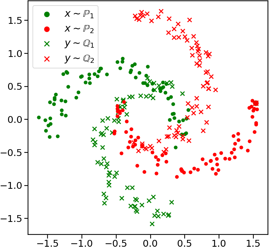
(a) $x\sim\mathbb{P}_{n}$ (circles),
$y\sim\mathbb{Q}_{n}$ (crosses).

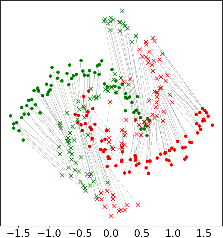
(b) Discrete OT-SI.

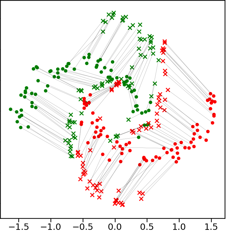
(c) Neural OT ($\ell^{2}$)

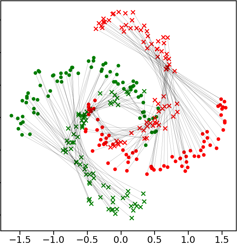
(d) Ours ($\mathcal{F}_{\text{G}}$)

Figure 2: The results of mapping two moons using OT with different cost functionals.

5 Experimental Illustrations

In this section, we test our continuous general OT approach with our cost functional $\mathcal{F}_{\text{G}}$ on toy cases (5.1) and image data (5.2). The code is written in PyTorch framework and will be made public along with the trained networks. On the image data, our method converges in 5–15 hours on a Tesla V100 (16 GB). We give the details (architectures, pre-processing, etc.) in Appendix C.1.

Our Algorithm 1 learns stochastic (one-to-many) transport maps $T(x,z)$. Following (Korotin et al., 2021b, 5), we also test deterministic $T(x,z)\equiv T(x)$, i.e., do not add a random noise $z$ to input. This disables stochasticity and yields deterministic (one-to-one) transport maps $x\mapsto T(x)$. In 5.1, (toy examples), we test only the deterministic variant of our method. In 5.2, we test both cases.

5.1 Toy Examples

The moons. The task is to map two balanced classes of moons (red and green) between $\mathbb{P}$ and $\mathbb{Q}$ (circles and crosses in Figure 2(a), respectively). The target distribution $\mathbb{Q}$ is $\mathbb{P}$ rotated by $90$ degrees. The number of randomly picked labelled samples in each target moon is 10. The maps learned by neural OT algorithm with the quadratic cost ($\mathbb{W}_{2}$, (Korotin et al., 2023b; Rout et al., 2022; Fan et al., 2021a)) and our Algorithm 1 with functional $\mathcal{F}_{\text{G}}$ are given in Figures 2(c) and 2(d), respectively. In Figure 2(b) we show the matching performed by a discrete OT-SI algorithm which learns the transport cost with a neural net from a known classes’ correspondence (Liu et al., 2020). As expected, the map for $\mathbb{W}_{2}$ does not preserve the classes (Figure 2(c)), while our map solves the task (Figure 2(d)). We provide an additional example with matching Gaussian Mixutres and solving the batch effect on biological data in Appendices  C.1 and C.9, respectively.

5.2 Image Data Experiments

Datasets. We use MNIST (LeCun & Cortes, 2010), FashionMNIST (Xiao et al., 2017) and KMNIST (Clanuwat et al., 2018) datasets as $\mathbb{P},\mathbb{Q}$. Each dataset has 10 (balanced) classes and the pre-defined train-test split. In this experiment, the goal is to find a class-wise map between unrelated domains: MNIST $\rightarrow$ KMNIST and FashionMNIST $\rightarrow$ MNIST. We use the default class correspondence between the datasets. For completeness, in Appendices we provide additional results with imbalanced classes (C.6), non-default correspondence (C.8), and mapping related domains (C.1).

Baselines: Well known conditional models, e.g., GAN (Mirza & Osindero, 2014), Adversarial Autoencoder (Makhzani et al., 2015), use the class labels to apply conditional generation. Due to that, they are not relevant to our work as we use only partial labeling information during the training and do not use any label information during the inference. For the same reason, a contrastive-penalty neural OT (Fan et al., 2023, 6.2) is also not relevant. Our learned mapping is based only on the input content. Domain adaptation methods (Gretton et al., 2012; Long et al., 2015; 2017; Ganin & Lempitsky, 2015; Long et al., 2018) align probability distributions while maintaining the discriminativity between classes (Wang & Deng, 2018). But mostly they perform domain adaptation for image data at the feature level and are typically not used at the pixel level (data space), which makes them also not relevant to the dataset transfer problem.

Due to that, we compare our method to the pixel-level adaptation methods that are typically based on the common unsupervised image-to-image translation techniques such as CycleGAN (Zhu et al., 2017; Hoffman et al., 2018; Almahairi et al., 2018) and UNIT (Huang et al., 2018; Liu et al., 2017). We consider (one-to-many) AugCycleGAN (Almahairi et al., 2018), MUNIT (Huang et al., 2018). We use the official implementations with the hyperparameters from the respective papers. Also, we test Neural OT (Korotin et al., 2023b; Fan et al., 2023) with Euclidean cost functions: the quadratic cost $\frac{1}{2}\|x-y\|_{2}^{2}$ ($\mathbb{W}_{2}$) and the $\gamma$-weak (one-to-many) quadratic cost ($\mathcal{W}_{2,\gamma}$, $\gamma=\frac{1}{10}$). The above-mentioned methods are unsupervised, i.e., they do not use the label information. Additionally, we add (one-to-one) OTDD flow (Alvarez-Melis & Fusi, 2021; 2020). This method employs gradient flows to perform the transfer preserving the class label. We also add a Discrete OT (DOT) method with the general cost. We employ the Sinkhorn (Cuturi, 2013) with Laplacian regularization for semi-supervised mapping (Courty et al., 2016) from ot.da package (Flamary et al., 2021) with its default out-of-sample estimation procedure. For completeness, we show the results of ICNN-based OT method (Makkuva et al., 2020; Korotin et al., 2021a) in Appendix C.7.

Metrics. All the models are fitted on the train parts of datasets; all the provided qualitative and quantitative results are exclusively for test (unseen) data. To evaluate the visual quality, we compute FID (Heusel et al., 2017) of the mapped source test set w.r.t. the target test set. To estimate the accuracy of the mapping we pre-train ResNet18 (He et al., 2016) classifier on the target data. We consider the mapping $T$ to be correct if the predicted label for the mapped sample $T(x,z)$ matches the corresponding label of $x$.

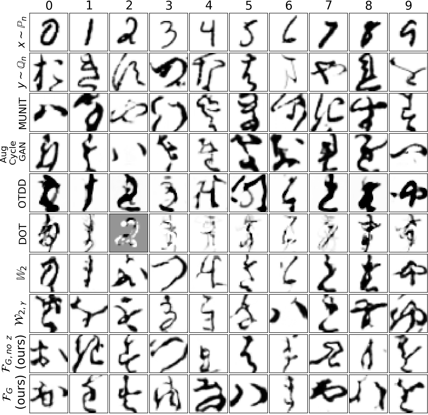
(a) MNIST $\rightarrow$ KMNIST

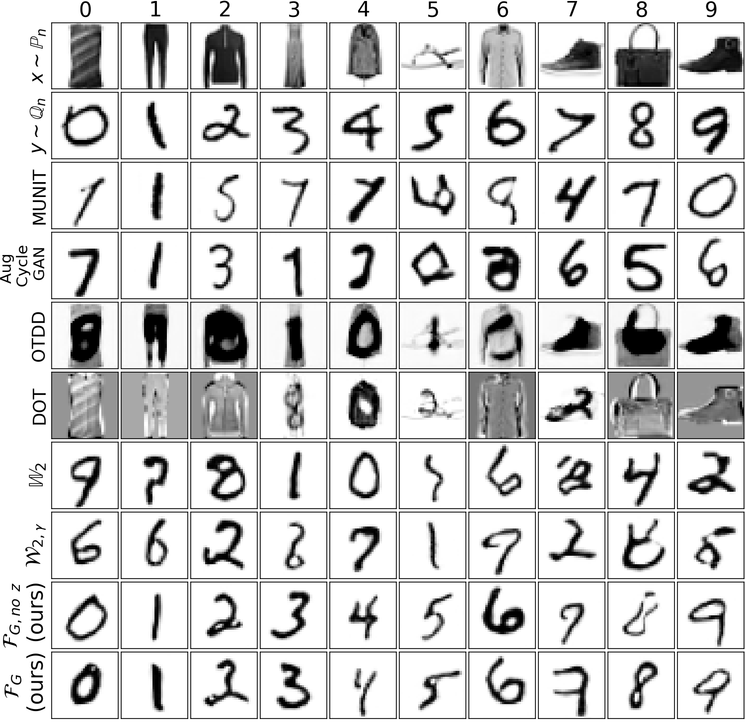
(b) FMNIST $\rightarrow$ MNIST

Figure 3: The results of mapping between two notably different datasets (unrelated domains).

	Image-to-Image Translation		Flows	Discrete OT	Neural Optimal Transport
Datasets ($32\times 32$)	MUNIT	Aug CycleGAN	OTDD	SinkhornLpL1	$\mathbb{W}_{2}$	$\mathcal{W}_{2,\gamma}$	$\mathcal{F}_{\text{G}}$, no $z$ [Ours]	$\mathcal{F}_{\text{G}}$ [Ours]
MNIST $\rightarrow$ KMNIST	12.27	8.99	4.46	4.27	6.13	6.82	79.20	61.91
FMNIST $\rightarrow$ MNIST	8.93	12.03	10.28	10.67	10.96	8.02	82.79	83.22

Table 1: Accuracy$\uparrow$ of the maps learned by the translation methods in view.

Datasets ($32\times 32$)	MUNIT	Aug CycleGAN	OTDD	SinkhornLpL1	$\mathbb{W}_{2}$	$\mathcal{W}_{2,\gamma}$	$\mathcal{F}_{\text{G}}$, no $z$ [Ours]	$\mathcal{F}_{\text{G}}$ [Ours]
MNIST $\rightarrow$ KMNIST	8.81	62.19	$>$ 100	40.96	12.85	9.46	17.26	9.69
FMNIST $\rightarrow$ MNIST	7.91	26.35	$>$ 100	$>$ 100	7.51	7.02	7.14	5.26

Table 2: FID$\downarrow$ of the samples generated by the translation methods in view.

Results. Qualitative results are shown in Figure 3; FID, accuracy – in Tables 2 and 1, respectively. To keep the figures simple, for all the models (one-to-one, one-to-many), we plot a single output per input. For completeness, we show multiple outputs per each input for our method and ablation study on $Z$ size in Appendices C.4 and  C.5. Our method, general discrete OT and OTDD, use 10 labeled samples for each class in the target. Other baselines lack the capability to use label information.

As seen in Figure 3 and Table 1, our approach using our cost $\mathcal{F}_{\text{G}}$ preserves the class-wise structure accurately with just 10 labelled samples per class. The accuracy of other neural OT methods is around $10\%$, equivalent to a random guess. Both the general discrete OT and OTDD methods do not preserve the class structure in high dimensions, resulting in samples with poor FID, see table 2. Visually, the OTDD results are comparable to those in Figure 3 of (Alvarez-Melis & Fusi, 2021).

6 Discussion

Potential Impact. Our method is a generic tool to learn transport maps between data distributions with a task-specific cost functional $\mathcal{F}$. Our method has promising positive real-world applications, such as digital content creation and artistic expression. At the same time, generative models can also be used for negative data manipulation purposes such as deepfakes. In general, the impact of our work on society depends on the scope of its application.

Limitations. To apply our method, one has to provide an estimator $\widehat{\mathcal{F}}(T)$ for the functional $\mathcal{F}$ which may be non-trivial. Besides, the construction of a cost functional $\mathcal{F}$ for a particular downstream task may be not straightforward. This should be taken into account when using the method in practice. Constructing task-specific functionals $\mathcal{F}$ and estimators $\widehat{\mathcal{F}}$ is a promising future research avenue.

7 Reproducibility

To ensure the reproducibility of our experiments, we provide the source code in the supplementary material. For toy experiments 5.1, run twomoons_toy.ipynb and gaussian_toy.ipynb. For the dataset transfer experiments 5.2, run dataset_transfer.ipynb and dataset_transfer_no_z.ipynb. The detailed information about the data preprocessing and training hyperparameters is presented in 5 and Appendix C.1.

Appendix A Proofs

A.1 Proofs of Results of 3

Proof of Theorem 1.

We use the dual form (5) to derive

$$\mbox{Cost}(\mathbb{P},\mathbb{Q})=\sup_{v}\left\{\sup_{u}\left[\int_{\mathcal{X}}u(x)d\mathbb{P}(x)-\mathcal{F}^{*}(u\oplus v)\right]+\int_{\mathcal{Y}}v(y)d\mathbb{Q}(y)\right\}=$$ (15)

$$\sup_{v}\left\{\sup_{u}\left[\int_{\mathcal{X}}u(x)d\mathbb{P}(x)-\sup_{\pi}\left(\int_{\mathcal{X}\times\mathcal{Y}}(u\oplus v)d\pi(x,y)-\mathcal{F}(\pi)\right)\right]+\int_{\mathcal{Y}}v(y)d\mathbb{Q}(y)\right\}=$$ (16)

$$\sup_{v}\left\{\sup_{u}\left[\int_{\mathcal{X}}u(x)d\mathbb{P}(x)+\inf_{\pi}\left(\mathcal{F}(\pi)-\int_{\mathcal{X}\times\mathcal{Y}}(u\oplus v)d\pi(x,y)\right)\right]+\int_{\mathcal{Y}}v(y)d\mathbb{Q}(y)\right\}=$$ (17)

$$\sup_{v}\left\{\sup_{u}\inf_{\pi}\left(\mathcal{F}(\pi)-\int_{\mathcal{X}}u(x)d\big{(}\pi-\mathbb{P})(x)-\int_{\mathcal{Y}}v(y)d\pi(y)\right)+\int_{\mathcal{Y}}v(y)d\mathbb{Q}(y)\right\}\leq$$ (18)

$$\sup_{v}\left\{\sup_{u}\inf_{\pi\in\Pi(\mathbb{P})}\left(\mathcal{F}(\pi)-\int_{\mathcal{X}}u(x)d\big{(}\pi-\mathbb{P})(x)-\int_{\mathcal{Y}}v(y)d\pi(y)\right)+\int_{\mathcal{Y}}v(y)d\mathbb{Q}(y)\right\}=$$ (19)

$$\sup_{v}\left\{\sup_{u}\inf_{\pi\in\Pi(\mathbb{P})}\left(\mathcal{F}(\pi)-\int_{\mathcal{Y}}v(y)d\pi(y)\right)+\int_{\mathcal{Y}}v(y)d\mathbb{Q}(y)\right\}=$$ (20)

$$\sup_{v}\left\{\inf_{\pi\in\Pi(\mathbb{P})}\left(\mathcal{F}(\pi)-\int_{\mathcal{Y}}v(y)d\pi(y)\right)+\int_{\mathcal{Y}}v(y)d\mathbb{Q}(y)\right\}\leq$$ (21)

$$\sup_{v}\bigg{\{}\mathcal{F}(\pi^{*})-\int_{\mathcal{Y}}v(y)\underbrace{d\pi^{*}(y)}_{d\mathbb{Q}(y)}+\int_{\mathcal{Y}}v(y)d\mathbb{Q}(y)\bigg{\}}=\mathcal{F}(\pi^{*})=\text{Cost}(\mathbb{P},\mathbb{Q}).$$ (22)

In line (15), we group the terms involving the potential $u$. In line (16), we express the conjugate functional $\mathcal{F}^{*}$ by using its definition. In the transition to line (17), we replace $\inf_{\pi}$ operator with the equivalent $\sup_{\pi}$ operator with the changed sign. In transition to (18), we put the term $\int_{\mathcal{X}}u(x)d\mathbb{P}(x)$ under the $\inf_{\pi}$ operator; we use definition $(u\oplus v)(x,y)=u(x)+v(y)$ to split the integral over $\pi(x,y)$ into two separate integrals over $\pi(x)$ and $\pi(y)$ respectively. In transition to (19), we restrict the inner $\inf_{\pi}$ to probability distributions $\pi\in\Pi(\mathbb{P})$ which have $\mathbb{P}$ as the first marginal, i.e. $d\pi(x)=d\mathbb{P}(x)$. This provides an upper bound on (18), in particular, all $u$-dependent terms vanish, see (20). As a result, we remove the $\sup_{u}$ operator in line (21). In transition to line (22) we substitute an optimal plan $\pi^{*}\in\Pi(\mathbb{P},\mathbb{Q})\subset\Pi(\mathbb{Q})$ to upper bound (21). Since $\text{Cost}(\mathbb{P},\mathbb{Q})$ turns to be both an upper bound (22) and a lower bound (15) for (21), we conclude that (6) holds. ∎

Proof of Theorem 7.

Assume that $\pi^{*}\notin\operatorname*{arg\,inf}_{\pi\in\Pi(\mathbb{P})}\mathcal{L}(v^{*},\pi)$, i.e.,

$${\mathcal{L}(v^{*},\pi^{*})>\inf_{\pi\in\Pi(\mathbb{P})}\mathcal{L}(v^{*},\pi)=\text{Cost}(\mathbb{P},\mathbb{Q})}.$$

We substitute $v^{*}$ and $\pi^{*}$ to $\mathcal{L}$ and see that

$$\mathcal{L}(v^{*},\pi^{*})=\big{[}\mathcal{F}(\pi^{*})-\int_{\mathcal{Y}}v(y)\underbrace{d\pi^{*}(y)}_{d\mathbb{Q}(y)}]\!+\!\int_{\mathcal{Y}}v(y)d\mathbb{Q}(y)=\mathcal{F}(\pi^{*})=\text{Cost}(\mathbb{P},\mathbb{Q}),$$

which is a contradiction. Thus, the assumption is wrong and (7) holds. ∎

Definition 1 (Strongly convex functional w.r.t. metric $\rho(\cdot,\cdot)$).

Let $\mathcal{F}:\mathcal{M}(\mathcal{X}\times\mathcal{Y})\rightarrow\mathbb{R}\cup\{+\infty\}$ be a convex lower semi-continuous functional. Let $\mathcal{U}\subset\mathcal{P}(\mathcal{X}\times\mathcal{Y})\subset\mathcal{M}(\mathcal{X}\times\mathcal{Y})$ be a convex subset such that $\exists\pi\in\mathcal{U}:\mathcal{F}(\pi)<+\infty$. Functional $\mathcal{F}$ is called $\beta$-strongly convex on $\mathcal{U}$ w.r.t. metric $\rho(\cdot,\cdot)$ if $\forall\pi_{1},\pi_{2}\in\mathcal{U},\forall\alpha\in[0,1]$ it holds:

$$\mathcal{F}(\alpha\pi_{1}+(1-\alpha)\pi_{2})\leq\alpha\mathcal{F}(\pi_{1})+(1-\alpha)\mathcal{F}(\pi_{2})-\frac{\beta}{2}\alpha(1-\alpha)\rho^{2}(\pi_{1},\pi_{2}).$$ (23)

Lemma 1 (Property of minimizers of strongly convex cost functionals).

Consider a lower-semicontinuous $\beta$-strongly convex in metric $\rho(\cdot,\cdot)$ on $\mathcal{U}\subset\mathcal{P}(\mathcal{X}\times\mathcal{Y})$ functional $\mathcal{F}$. Assume that $\pi^{*}\in\mathcal{U}$ satisfies $\mathcal{F}(\pi^{*})=\inf\limits_{\pi\in\mathcal{U}}\mathcal{F}(\pi)$. Then $\forall\pi\in\mathcal{U}$ it holds:

$$\mathcal{F}(\pi^{*})\leq\mathcal{F}(\pi)-\frac{\beta}{2}\rho^{2}(\pi^{*},\pi).$$ (24)

Proof of Lemma 1.

We substitute $\pi_{1}=\pi^{*}$, $\pi_{2}=\pi$ to formula (23) and fix $\alpha\in[0,1]$. We obtain

$$\mathcal{F}(\alpha\pi^{*}+(1-\alpha)\pi)\leq\alpha\mathcal{F}(\pi^{*})+(1-\alpha)\mathcal{F}(\pi)-\frac{\beta}{2}\alpha(1-\alpha)\rho^{2}(\pi^{*},\pi)\Longleftrightarrow$$

$$\underbrace{\mathcal{F}(\alpha\pi^{*}+(1-\alpha)\pi)}_{\geq\inf\limits_{\pi^{\prime}\in\mathcal{U}}\mathcal{F}(\pi^{\prime})=\mathcal{F}(\pi^{*})}-\alpha\mathcal{F}(\pi^{*})\leq(1-\alpha)\mathcal{F}(\pi)-\frac{\beta}{2}\alpha(1-\alpha)\rho^{2}(\pi^{*},\pi)\Longrightarrow$$

$$(1-\alpha)\mathcal{F}(\pi^{*})\leq(1-\alpha)\mathcal{F}(\pi)-\frac{\beta}{2}\alpha(1-\alpha)\rho^{2}(\pi^{*},\pi)\Longleftrightarrow$$

$$\mathcal{F}(\pi^{*})\leq\mathcal{F}(\pi)-\frac{\beta}{2}\alpha\rho^{2}(\pi^{*},\pi).$$ (25)

Taking the limit $\alpha\rightarrow 1-$ in inequality (25), we obtain (24). ∎

Proof of Theorem 3.

Given a potential $v\in\mathcal{C}(\mathcal{Y})$, we define functional $\mathcal{V}_{v}:\Pi(\mathbb{P})\rightarrow\mathbb{R}\cup\{+\infty\}$:

$$\mathcal{V}_{v}(\pi)\stackrel{{\scriptstyle\text{def}}}{{=}}\mathcal{F}(\pi)-\int_{\mathcal{Y}}v(y)d\pi(y).$$ (26)

Since the term $\int_{\mathcal{Y}}v(y)d\pi(y)$ is linear w.r.t. $\pi$, the $\beta$-strong convexity of $\mathcal{F}$ implies $\beta$-strong convexity of $\mathcal{V}_{v}$. Moreover, since $\mathcal{V}_{v}$ is lower semi-continuous and $\Pi(\mathbb{P})$ is compact (w.r.t. weak-$*$ topology), it follows from the Weierstrass theorem (Santambrogio, 2015, Box 1.1) that

$$\exists\pi^{v}\in\Pi(\mathbb{P}):\mathcal{V}_{v}(\pi^{v})=\inf\limits_{\pi\in\Pi(\mathbb{P})}\mathcal{V}_{v}(\pi);$$ (27)

i.e. the infimum of $\mathcal{V}_{v}(\pi)$ is attained. Note that $\pi^{v}$ minimizes the functional $\pi\mapsto\mathcal{L}(v,\pi)$ as well since $\mathcal{L}(v,\pi)=\mathcal{V}_{v}(\pi)+\text{Const}(v)$. Therefore, the duality gaps (9), (10) permit the following reformulation:

$$\epsilon_{1}(\hat{v},\hat{\pi})=\mathcal{L}(\hat{v},\hat{\pi})-\mathcal{L}(\hat{v},\pi^{\hat{v}}),$$ (28)

$$\epsilon_{2}(\hat{v})=\mathcal{L}(v^{*},\pi^{*})-\mathcal{L}(\hat{v},\pi^{\hat{v}});$$ (29)

where $\pi^{\hat{v}}$ is a minimizer (27) for $v=\hat{v}$. Consider expression (28):

$$\epsilon_{1}(\hat{v},\hat{\pi})=\mathcal{L}(\hat{v},\hat{\pi})-\mathcal{L}(\hat{v},\pi^{\hat{v}})\stackrel{{\scriptstyle\text{Lemma \ref{lm-minprop}}}}{{\geq}}\frac{\beta}{2}\rho^{2}(\hat{\pi},\pi^{\hat{v}})\Longrightarrow$$

$$\sqrt{\frac{2}{\beta}\epsilon_{1}(\hat{v},\hat{\pi})}\geq\rho(\hat{\pi},\pi^{\hat{v}}).$$ (30)

Consider expression (29):

$$\epsilon_{2}(\hat{v})=\mathcal{L}(v^{*},\pi^{*})-\mathcal{L}(\hat{v},\pi^{\hat{v}})=$$

$$\mathcal{F}(\pi^{*})-\int_{\mathcal{Y}}v^{*}(y)d\big{(}\pi^{*}-\mathbb{Q}\big{)}(y)-\mathcal{F}(\pi^{\hat{v}})+\int_{\mathcal{Y}}\hat{v}(y)d\big{(}\pi^{\hat{v}}-\mathbb{Q}\big{)}(y)=$$

$$\mathcal{F}(\pi^{*})-\int_{\mathcal{Y}}\hat{v}(y)d(\pi^{*}-\mathbb{Q})(y)+\int_{\mathcal{Y}}\{\hat{v}(y)-v^{*}(y)\}d\big{(}\pi^{*}-\mathbb{Q}\big{)}(y)-\mathcal{F}(\pi^{\hat{v}})+\int_{\mathcal{Y}}\hat{v}(y)d\big{(}\pi^{\hat{v}}-\mathbb{Q}\big{)}(y)=$$ (31)

$$\underbrace{\mathcal{F}(\pi^{*})-\int_{\mathcal{Y}}\hat{v}(y)d\pi^{*}(y)}_{=\mathcal{V}_{\hat{v}}(\pi^{*})}+\underbrace{\int_{\mathcal{Y}}\{\hat{v}(y)-v^{*}(y)\}d\big{(}\pi^{*}-\mathbb{Q}\big{)}(y)}_{=0\text{, since }d\pi^{*}(y)=d\mathbb{Q}(y)}\underbrace{-\mathcal{F}(\pi^{\hat{v}})+\int_{\mathcal{Y}}\hat{v}(y)d\pi^{\hat{v}}(y)}_{=-\mathcal{V}_{\hat{v}}(\pi^{\hat{v}})}=$$

$$\mathcal{V}_{\hat{v}}(\pi^{*})-\mathcal{V}_{\hat{v}}(\pi^{\hat{v}})\stackrel{{\scriptstyle\text{Lemma \ref{lm-minprop}}}}{{\geq}}\frac{\beta}{2}\rho^{2}(\pi^{*},\pi^{\hat{v}})\Longrightarrow$$

$$\sqrt{\frac{2}{\beta}\epsilon_{2}(\hat{v})}\geq\rho(\pi^{*},\pi^{\hat{v}});$$ (32)

where in line (31) we add and subtract $\int_{\mathcal{Y}}\hat{v}(y)d(\pi^{*}-\mathbb{Q})(y)$.

The triangle inequality $\rho(\pi^{*},\hat{\pi})\leq\rho(\pi^{*},\pi^{\hat{v}})+\rho(\hat{\pi},\pi^{\hat{v}})=\sqrt{\frac{2}{\beta}}\left(\sqrt{\epsilon_{1}(\hat{v},\hat{\pi})}+\sqrt{\epsilon_{2}(\hat{v})}\right)$ for norm $\rho(\cdot,\cdot)$ finishes the proof. ∎

A.2 Proofs of Results of 1

Proof of Theorem 4.

First, we prove that $\mathcal{F}=\mathcal{F}_{\text{G}}$ it is *-separately increasing. For $\pi\in\mathcal{M}(\mathcal{X}\times\mathcal{Y})\setminus\Pi(\mathbb{P})$ it holds that $\mathcal{F}(\pi)=+\infty$. Consequently,

$$\int_{\mathcal{X}\times\mathcal{Y}}c(x,y)d\pi(x,y)-\mathcal{F}(\pi)=\int_{\mathcal{X}\times\mathcal{Y}}\big{(}u(x)+v(y)\big{)}d\pi(x,y)-\mathcal{F}(\pi)=-\infty.$$ (33)

When $\pi\in\Pi(\mathbb{P})$ it holds that $\pi$ is a probability distribution. We integrate $u(x)+v(y)\leq c(x,y)$ w.r.t. $\pi$, subtract $\mathcal{F}(\pi)$ and obtain

$$\int_{\mathcal{X}\times\mathcal{Y}}c(x,y)d\pi(x,y)-\mathcal{F}(\pi)\geq\int_{\mathcal{X}\times\mathcal{Y}}\big{(}u(x)+v(y)\big{)}d\pi(x,y)-\mathcal{F}(\pi).$$ (34)

By taking the $\sup$ of (33) and (34) w.r.t. $\pi\in\mathcal{M}(\mathcal{X}\times\mathcal{Y})$, we obtain $\mathcal{F}^{*}(c)\geq\mathcal{F}^{*}(u\oplus v)$.

Next, we prove that $\mathcal{F}$ is convex. We prove that every term $\mathcal{E}^{2}\big{(}T_{\pi}\sharp(\mathbb{P}_{n}\times\mathbb{S}),\mathbb{Q}_{n}\big{)}$ is convex in $\pi$.

First, we show that $\pi\mapsto f_{n}(\pi)\stackrel{{\scriptstyle def}}{{=}}T_{\pi}\sharp(\mathbb{P}_{n}\times\mathbb{S})$ is linear in $\pi\in\Pi(\mathbb{P})$.

Pick any ${\pi_{1},\pi_{2},\pi_{3}\in\Pi(\mathbb{P})}$ which lie on the same line. Without loss of generatity we assume that $\pi_{3}\in[\pi_{1},\pi_{2}]$, i.e., $\pi_{3}=\alpha\pi_{1}+(1-\alpha)\pi_{2}$ for some $\alpha\in[0,1]$. We need to show that

$$f_{n}(\pi_{3})=\alpha f_{n}(\pi_{1})+(1-\alpha)f_{n}(\pi_{2}).$$ (35)

In what follows, for a random variable $U$ we denote its distribution by $\text{Law}(U)$.

The first marginal distribution of each $\pi_{i}$ is $\mathbb{P}$. From the glueing lemma (Villani, 2008, 1) it follows that there exists a triplet of (dependent) random variables $(X,Y_{1},Y_{2})$ such that $\text{Law}(X,Y_{i})=\pi_{i}$ for $i=1,2$. We define ${Y_{3}=Y_{r}}$, where $r$ is an independent random variable which takes values in $\{1,2\}$ with probabilities $\{\alpha,1-\alpha\}$. From the construction of $Y_{3}$ it follows that $\text{Law}(X,Y_{3})$ is a mixture of $\text{Law}(X,Y_{1})=\pi_{1}$ and $\text{Law}(X,Y_{2})=\pi_{2}$ with weights $\alpha$ and $1-\alpha$. Thus, $\text{Law}(X,Y_{3})=\alpha\pi_{1}+(1-\alpha)\pi_{2}=\pi_{3}$. We conclude that $\text{Law}(Y_{3}|X\!=\!x)=\pi_{3}(\cdot|x)$ for $\mathbb{P}$-almost all $x\in\mathcal{X}$ (recall that $\text{Law}(X)\!=\!\mathbb{P}$). On the other hand, again by the construction, the conditional $\text{Law}(Y_{3}|X\!=\!x)$ is a mixture of $\text{Law}(Y_{1}|X\!=\!x)=\pi_{1}(\cdot|x)$ and $\text{Law}(Y_{2}|X\!=\!x)=\pi_{2}(\cdot|x)$ with weights $\alpha$ and $1-\alpha$. Thus, $\pi_{3}(\cdot|x)=\alpha\pi_{1}(\cdot|x)+(1-\alpha)\pi_{2}(\cdot|x)$ holds true for $\mathbb{P}$-almost all $x\in\mathcal{X}$.

Consider independent random variables $X_{n}\sim\mathbb{P}_{n}$ and $Z\sim\mathbb{S}$. From the definition of $T_{\pi_{i}}$ we conclude that $\text{Law}\big{(}T_{\pi_{i}}(x,Z)\big{)}=\pi_{i}(\cdot|x)$ for $\mathbb{P}$-almost all $x\in\mathcal{X}$ and, since $\mathbb{P}_{n}$ is a component of $\mathbb{P}$, for $\mathbb{P}_{n}$-almost all $x\in\mathcal{X}$ as well. As a result, we define $T_{i}=T_{\pi_{i}}(X_{n},Z)$ and derive

$$\text{Law}(T_{3}|X_{n}=x)=\pi_{3}(\cdot|x)=\alpha\pi_{1}(\cdot|x)+(1-\alpha)\pi_{2}(\cdot|x)=$$

$$\alpha\text{Law}(T_{1}|X_{n}=x)+(1-\alpha)\text{Law}(T_{2}|X_{n}=x)$$

for $\mathbb{P}_{n}$-almost all $x\in\mathcal{X}$. Thus, $\text{Law}(X_{n},T_{3})$ is also a mixture of $\text{Law}(X_{n},T_{1})$ and $\text{Law}(X_{n},T_{2})$ with weights $\alpha$ and $1-\alpha$. In particular, $\text{Law}(T_{3})=\alpha\text{Law}(T_{1})+(1-\alpha)\text{Law}(T_{2})$. We note that $\text{Law}(T_{i})=f_{n}(\pi_{i})$ by the definition of $f_{n}$ and obtain (35).

Second, we highlight that for every $\nu\in\mathcal{P}(\mathcal{Y})$, the functional $\mathcal{P}(\mathcal{Y})\ni\mu\rightarrow\mathcal{E}^{2}(\mu,\nu)$ is convex in $\mu$. Indeed, $\mathcal{E}^{2}$ is a particular case of (the square of) Maximum Mean Discrepancy (MMD, (Sejdinovic et al., 2013)). Therefore, there exists a Hilbert space $\mathcal{H}$ and a function $\phi:\mathcal{Y}\rightarrow\mathcal{H}$ (feature map), such that

$$\mathcal{E}^{2}(\mu,\nu)=\left\|\int_{\mathcal{Y}}\phi(y)d\mu(y)-\int_{\mathcal{Y}}\phi(y)d\nu(y)\right\|^{2}_{\mathcal{H}}.$$

Since the kernel mean embedding $\mu\mapsto\int_{\mathcal{Y}}\phi(y)d\mu(y)$ is linear in $\mu$ and $\|\cdot\|^{2}_{\mathcal{H}}$ is convex, we conclude that $\mathcal{E}^{2}(\mu,\nu)$ is convex in $\mu$. To finish this part of the proof, it remains to combine the fact that $\pi\mapsto T_{\pi}\sharp(\mathbb{P}_{n}\times\mathbb{S})$ is linear and $\mathcal{E}^{2}(\cdot,\mathbb{Q}_{n})$ is convex in the first argument.

Third, we note that the lower semi-continuity of $\mathcal{F}(\pi)$ in $\Pi(\mathbb{P})$ follows from the lower semi-continuity of the Energy distance ($\mathcal{E}^{2}$) terms in (12). That is, it suffices to show that $\mathcal{E}^{2}$ defined in equation (13) is indeed lower semi-continuous in the first argument $\mathbb{Q}_{1}$. In (13), there are two terms depending on $\mathbb{Q}_{1}$. The term $\mathbb{E}\|X_{1}-X_{1}^{\prime}\|_{2}=\int_{\mathcal{X}}\big{[}\int_{\mathcal{X}}\|x_{1}-x_{2}\|_{2}d\mathbb{Q}_{2}(x_{2})\big{]}d\mathbb{Q}_{1}(x_{1})$ is linear in $\mathbb{Q}_{1}$. It is just the expectation of a continuous function w.r.t. $\mathbb{Q}_{1}$. Hence it is lower semi-continuous by the definition of the lower semi-continuity. Here we also use the fact that $\mathcal{Y}$ is compact. The other term $-\frac{1}{2}\mathbb{E}\|X_{1}-X_{1}^{\prime}\|_{2}=-\frac{1}{2}\int_{\mathcal{X}\times\mathcal{X}}\|x_{2}-x_{2}^{\prime}\|_{2}d\big{(}\mathbb{Q}_{1}\times\mathbb{Q}_{1}\big{)}(x_{1},x_{2})$ is a quadratic term in $\mathbb{Q}_{1}$. This term can be viewed as the interaction energy (Santambrogio, 2015, 7) between particles in $\mathbb{Q}_{1}$ with the interaction function $W(x_{1},x_{1}^{\prime})\stackrel{{\scriptstyle def}}{{=}}-\|x_{1}-x_{1}^{\prime}\|_{2}$. Thanks to the compactness of $\mathcal{Y}$, it is also lower semi-continuous in $\mathbb{Q}_{1}$, see (Santambrogio, 2015, Proposition 7.2) for the proof. ∎

Proof of Proposition 1.

Direct calculation of the expectation of (14) yields the value

$$\mathbb{E}\|Y-T(X,Z)\|_{2}-\frac{1}{2}\mathbb{E}\|T(X,Z)-T(X^{\prime},Z^{\prime})\|_{2}=$$

$$\mathbb{E}\|Y-T(X,Z)\|-\frac{1}{2}\mathbb{E}\|T(X,Z)-T(X^{\prime},Z^{\prime})\|_{2}-\frac{1}{2}\mathbb{E}\|Y-Y^{\prime}\|_{2}+\frac{1}{2}\mathbb{E}\|Y-Y^{\prime}\|_{2}=$$

$$\mathcal{E}^{2}\big{(}T\sharp(\mathbb{P}_{n}\times\mathbb{S}),\mathbb{Q}_{n}\big{)}+\frac{1}{2}\mathbb{E}\|Y-Y^{\prime}\|_{2},$$ (36)

where $Y,Y^{\prime}\sim\mathbb{Q}_{n}$ and $(X,Z),(X^{\prime},Z^{\prime})\sim(\mathbb{P}_{n}\times\mathbb{S})$ are independent random variables. It remains to note that $\frac{1}{2}\mathbb{E}\|Y-Y^{\prime}\|_{2}$ is a $T$-independent constant. ∎

Appendix B Algorithm for General Cost Functionals

In this section, we present the procedure to optimize (2) for general cost functionals $\mathcal{F}$. In practice, one may utilize neural networks $T_{\theta}:\mathbb{R}^{D}\times\mathbb{R}^{S}\rightarrow\mathbb{R}^{D}$ and $v_{\omega}:\mathbb{R}^{D}\rightarrow\mathbb{R}$ to parameterize $T$ and $v_{\omega}$, correspondingly, to solve the problem (2). One may train them with stochastic gradient ascent-descent (SGAD) using random batches from $\mathbb{P},\mathbb{Q},\mathbb{S}$. The procedure is summarized in Algorithm 2.

Input : Distributions $\mathbb{P},\mathbb{Q},\mathbb{S}$ accessible by samples; mapping network $T_{\theta}:\mathbb{R}^{P}\times\mathbb{R}^{S}\rightarrow\mathbb{R}^{Q}$; potential network $v_{\omega}:\mathbb{R}^{Q}\rightarrow\mathbb{R}$; number of inner iterations $K_{T}$; empirical estimator $\widehat{\mathcal{F}}\big{(}X,T(X,Z)\big{)}$ for cost $\widetilde{\mathcal{F}}(T)$;

Output : Learned stochastic OT map $T_{\theta}$ representing an OT plan between distributions $\mathbb{P},\mathbb{Q}$;

repeat

     Sample batches $Y\sim\mathbb{Q}$, $X\sim\mathbb{P}$ and for each $x\in X$ sample batch $Z[x]\sim\mathbb{S}$;

     ${\mathcal{L}_{v}\leftarrow\sum\limits_{x\in X}\sum\limits_{z\in Z[x]}\frac{v_{\omega}(T_{\theta}(x,z))}{|X|\cdot|Z[x]|}-\sum\limits_{y\in Y}\frac{v_{\omega}(y)}{|Y|}}$;

    

    Update $\omega$ by using $\frac{\partial\mathcal{L}_{v}}{\partial\omega}$;

    

    for $k_{T}=1,2,\dots,K_{T}$ do

         Sample batch $X\sim\mathbb{P}$ and for each $x\in X$ sample batch $Z[x]\sim\mathbb{S}$;

         ${\mathcal{L}_{T}\leftarrow\widehat{\mathcal{F}}(X,T_{\theta}(X,Z))-\sum\limits_{x\in X}\sum\limits_{z\in Z[x]}\frac{v_{\omega}(T_{\theta}(x,z))}{|X|\cdot|Z[x]|}}$;

         Update $\theta$ by using $\frac{\partial\mathcal{L}_{T}}{\partial\theta}$;

        

    

until not converged;

Algorithm 2 Neural optimal transport for general cost functionals

Algorithm 2 requires an empirical estimator $\widehat{\mathcal{F}}$ for $\widetilde{\mathcal{F}}(T)$. Providing such an estimator might be non-trivial for general $\mathcal{F}$. If $\mathcal{F}(\pi)=\int_{\mathcal{X}}C(x,\pi(\cdot|x))d\mathbb{P}(x)$, i.e., the cost is weak (2), one may use the following unbiased Monte-Carlo estimator: $\widehat{\mathcal{F}}\big{(}X,T(X,Z)\big{)}\stackrel{{\scriptstyle def}}{{=}}|X|^{-1}\sum_{x\in X}\widehat{C}\big{(}x,T(x,Z[x])\big{)},$ where $\widehat{C}$ is the respective estimator for the weak cost $C$ and $Z[x]$ denotes a random batch of latent vectors $z\sim\mathbb{S}$ for a given $x\in\mathcal{X}$. For classic costs and the $\gamma$-weak quadratic cost, the estimator $\widehat{C}$ is given by (Korotin et al., 2023b, Eq. 18 and 19) and Algorithm 2 for general OT 4 reduces to the neural OT algorithm (Korotin et al., 2023b, Algorithm 1) for weak (2) or classic (1) OT. Unlike the predecessor, the algorithm is suitable for general OT formulation (4). In 1, we propose a cost functional $\mathcal{F}_{\text{G}}$ and provide an estimator for it to solve the class-guided dataset transfer task (Algorithm 1).

Appendix C Additional Experiments

C.1 Training Details of the Main Experiments

Algorithm details. In our Algorithm 1, we use Adam (Kingma & Ba, 2014) optimizer with $lr=10^{-4}$ for both $T_{\theta}$ and $v_{\omega}$. The number of inner iterations for $T_{\theta}$ is $K_{T}=10$. Doing preliminary experiments, we noted that it is sufficient to use small mini-batch sizes $K_{X},K_{Y},K_{Z}$ in (14). Therefore, we decided to average loss values over $K_{B}$ small independent mini-batches (each from class $n$ with probability $\alpha_{n}$) rather than use a single large batch from one class. This is done parallel with tensor operations.

Two moons. We use 500 train and 150 test samples for each moon. We use the fully-connected net with 2 ReLU hidden layers size of 128 for both $T_{\theta}$ and $v_{\omega}$. We train the model for 10k iterations of $v_{\omega}$ with $K_{B}=32,K_{X}=K_{Y}=2$ ($K_{Z}$ plays no role as we do not use $z$ here).

Images experiments details. We rescale the images to size 32×32 and normalize their channels to $[-1,1]$. For the grayscale images, we repeat their channel $3$ times and work with $3$-channel images. We do not apply any augmentations to data. We use the default train-test splits for all the datasets.

We use WGAN-QC discriminator’s ResNet architecture (He et al., 2016) for potential $v_{\omega}$. We use UNet (Ronneberger et al., 2015) as the stochastic transport map $T_{\theta}(x,z)$. To condition it on $z$, we insert conditional instance normalization (CondIN) layers after each UNet’s upscaling block. We use CondIN from AugCycleGAN (Almahairi et al., 2018). In experiments, $z$ is the 128-dimensional standard Gaussian noise.

The batch size is $K_{B}=32$, $K_{X}=K_{Y}=2$, $K_{Z}=2$ for training with $z$. When training without $z$, we use the original UNet without conditioning; the batch parameters are the same ($K_{Z}$ does not matter). Our method converges in $\approx 60$k iterations of $v_{\omega}$.

For comparison in the image domain, we use the official implementations with the hyperparameters from the respective papers: AugCycleGAN (Almahairi et al., 2018), MUNIT(Huang et al., 2018). For comparison with neural OT ($\mathbb{W}_{2},\mathcal{W}_{2,\gamma}$), we use their publicly available code.

OTDD flow details. As in our method, the number of labelled samples in each class is 10. We learn the OTDD flow between the labelled source dataset and labelled target samples. Note the OTDD method does not use the unlabeled target samples. As the OTDD method does not produce out-of-sample estimates, we train UNet to map the source data to the data produced by the OTDD flow via regression. Then we compute the metrics on the test (FID, accuracy) for this mapping network.

DOT details. Input pre-processing was the same as in our method. We tested a variety of discrete OT solvers from Python Optimal Transport (POT) package (Flamary et al., 2021), including EMD, MappingTransport (Perrot et al., 2016) and SinkhornTransport with Laplacian and L2 regularization (Courty et al., 2016) from ot.da (Flamary et al., 2021). These methods are semi-supervised and can receive labels to construct a task-specific plan. As in our method, the number of labelled samples in each class is 10. For most of these methods, two tunable hyper-parameters are available: entropic and class regularization values. We evaluated a range of these values (1, 2, 5, 10, and 100). To assess the accuracy of the DOT solvers, we used the same oracle classifiers as in all the other cases. Empirically, we found that Sinkhorn with Laplacian regularization and both regularization values equal to 5 achieves the best performance in most cases. Thus, to keep Table 1 simple, we report the test accuracy results only for this DOT approach. Additionally, we calculated its test FID (Table 2).

C.2 Gaussians Mixtures.

In this additional experiment both $\mathbb{P},\mathbb{Q}$ are balanced mixtures of 16 Gaussians, and each color denotes a unique class. The goal is to map Gaussians in $\mathbb{P}$ (Figure 4(a)) to respective Gaussians in $\mathbb{Q}$ which have the same color, see Figure  4(b). The result of our method 10 known target labels per class) is given in Figure 4(c). It correctly maps the classes. Neural OT for the quadratic cost is not shown as it results in the identity map (the same image as Figure 4(a)) which is completely mistaken in classes. We use the fully connected network with 2 ReLU hidden layers size of 256 for both $T_{\theta}$ and $v_{\omega}$. There are 10000 train and 500 test samples in each Gaussian. We train the model for 10k iterations of $v_{\omega}$ with $K_{B}=32,K_{X}=K_{Y}=2$ ($K_{Z}$ plays no role here as well).

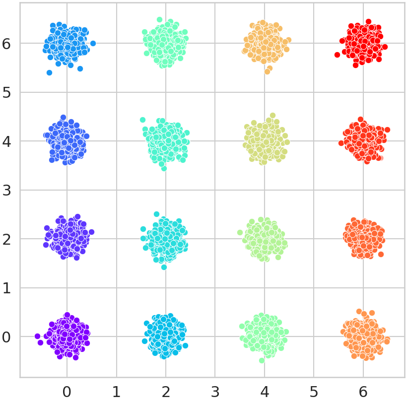
(a) Input $x\sim\mathbb{P}$.

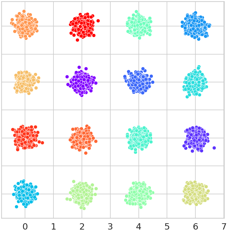
(b) Target $y\sim\mathbb{Q}$.

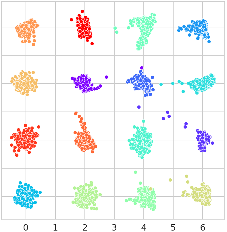
(c) Ours ($\mathcal{F}_{\text{G}}$)

Figure 4: Illustration of the mapping between two Gaussian mixtures learned by our Algorithm 1.

C.3 Related Domains

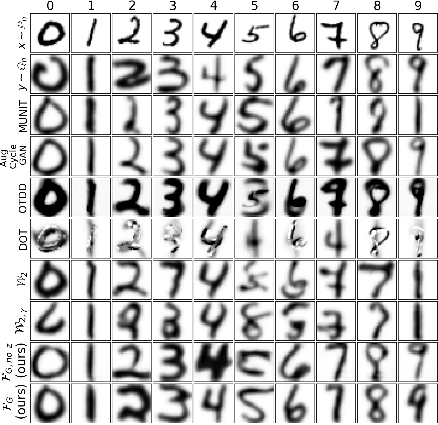
(a) MNIST $\rightarrow$ USPS

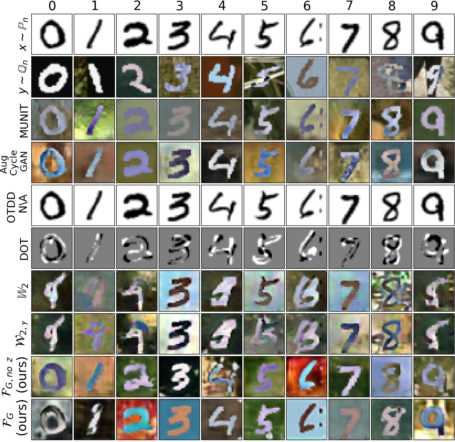
(b) MNIST $\rightarrow$ MNIST-M

Figure 5: The results of mapping between two similar images datasets (related domains).

	Image-to-Image Translation		Flows	Discrete OT	Neural Optimal Transport
Datasets ($32\times 32$)	MUNIT	Aug CycleGAN	OTDD	SinkhornLpL1	$\mathbb{W}_{2}$	$\mathcal{W}_{2,\gamma}$	$\mathcal{F}_{\text{G}}$, no $z$ [Ours]	$\mathcal{F}_{\text{G}}$ [Ours]
MNIST $\rightarrow$ USPS	82.97	96.52	82.50	49.13	56.27	34.33	93.42	95.14
MNIST $\rightarrow$ MNIST-M	97.95	98.2	-	83.26	38.77	37.0	95.27	94.62

Table 3: Accuracy$\uparrow$ of the maps learned by the translation methods in view.

Datasets ($32\times 32$)	MUNIT	Aug CycleGAN	OTDD	SinkhornLpL1	$\mathbb{W}_{2}$	$\mathcal{W}_{2,\gamma}$	$\mathcal{F}_{\text{G}}$, no $z$ [Ours]	$\mathcal{F}_{\text{G}}$ [Ours]
MNIST $\rightarrow$ USPS	6.86	22.74	$>$ 100	51.18	4.60	3.05	5.40	2.87
MNIST $\rightarrow$ MNIST-M	11.68	26.87	-	$>$ 100	19.43	17.48	18.56	6.67

Table 4: FID$\downarrow$ of the samples generated by the translation methods in view.

Here we test the case when the source and target domains are related. We consider MNIST$\rightarrow$USPS and MNIST$\rightarrow$MNISTM translation. As in the main text, we are given only 10 labeled samples from the target dataset; the rest are unlabeled. The results are in Table 3, 4 and Figure 5.

In this related domains case (Figure 5), GAN-based methods and our approach with our guided cost $\mathcal{F}_{\text{G}}$ show high accuracy $\geq 90\%$. However, neural OT with classic and weak quadratic costs provides low accuracy (35-50%). We presume that this is because for these dataset pairs the ground truth OT map for the (pixel-wise) quadratic cost simply does not preserve the class. This agrees with (Daniels et al., 2021, Figure 3) which tests an entropy-regularized quadratic cost in a similar MNIST$\rightarrow$USPS setup. For our method with cost $\mathcal{F}_{\text{G}}$, The OTDD gradient flows method provides reasonable accuracy on MNIST$\rightarrow$USPS. However, OTDD has a much higher FID than the other methods.

C.4 Additional Examples of Stochastic Maps

In this subsection, we provide additional examples of the learned stochastic map for $\mathcal{F}_{\text{G}}$ (with $z$). We consider all the image datasets from the main experiments (5). The results are shown in Figure 7 and demonstrate that for a fixed $x$ and different $z$, our model generates diverse samples.

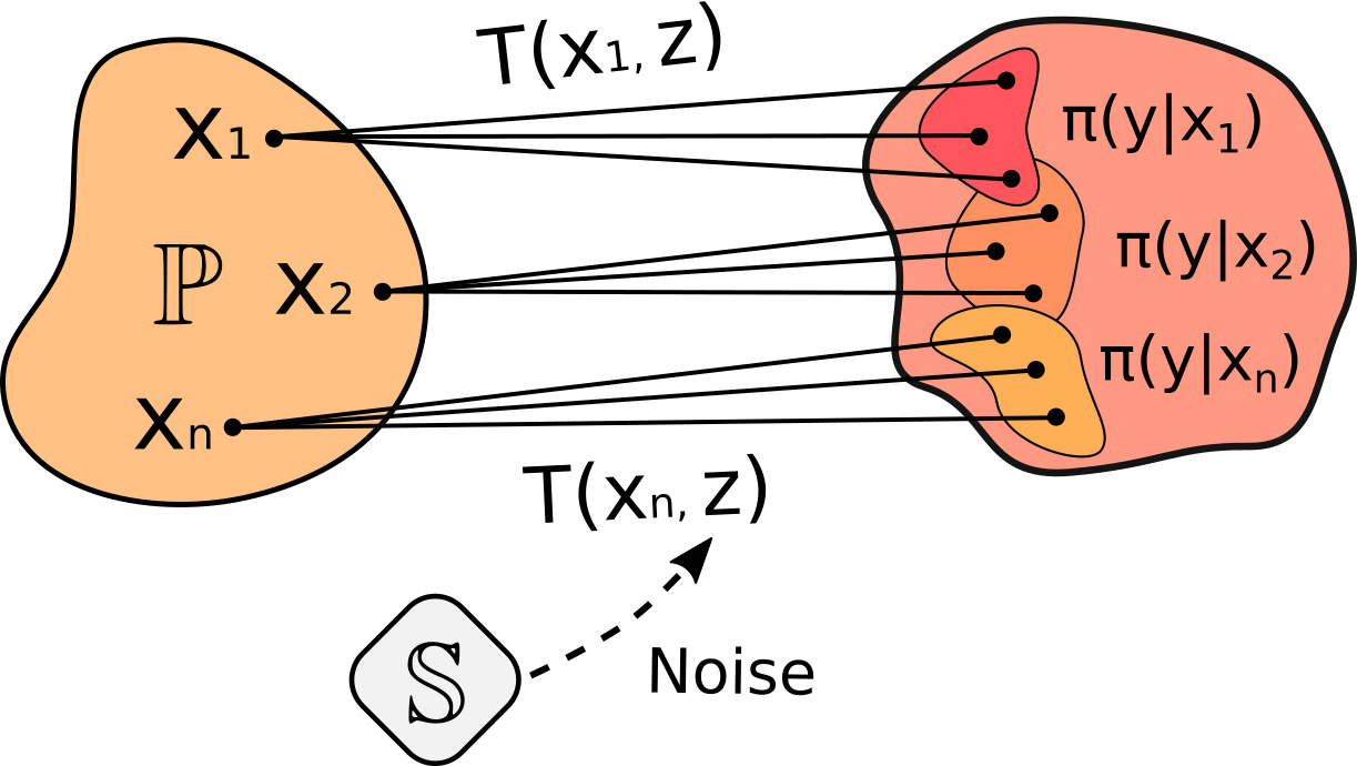
Figure 6: Implicit representation of $\pi\in\Pi(\mathbb{P})$ via function $T=T_{\pi}:\mathcal{X}\!\times\!\mathcal{Z}\rightarrow\mathcal{Y}$.

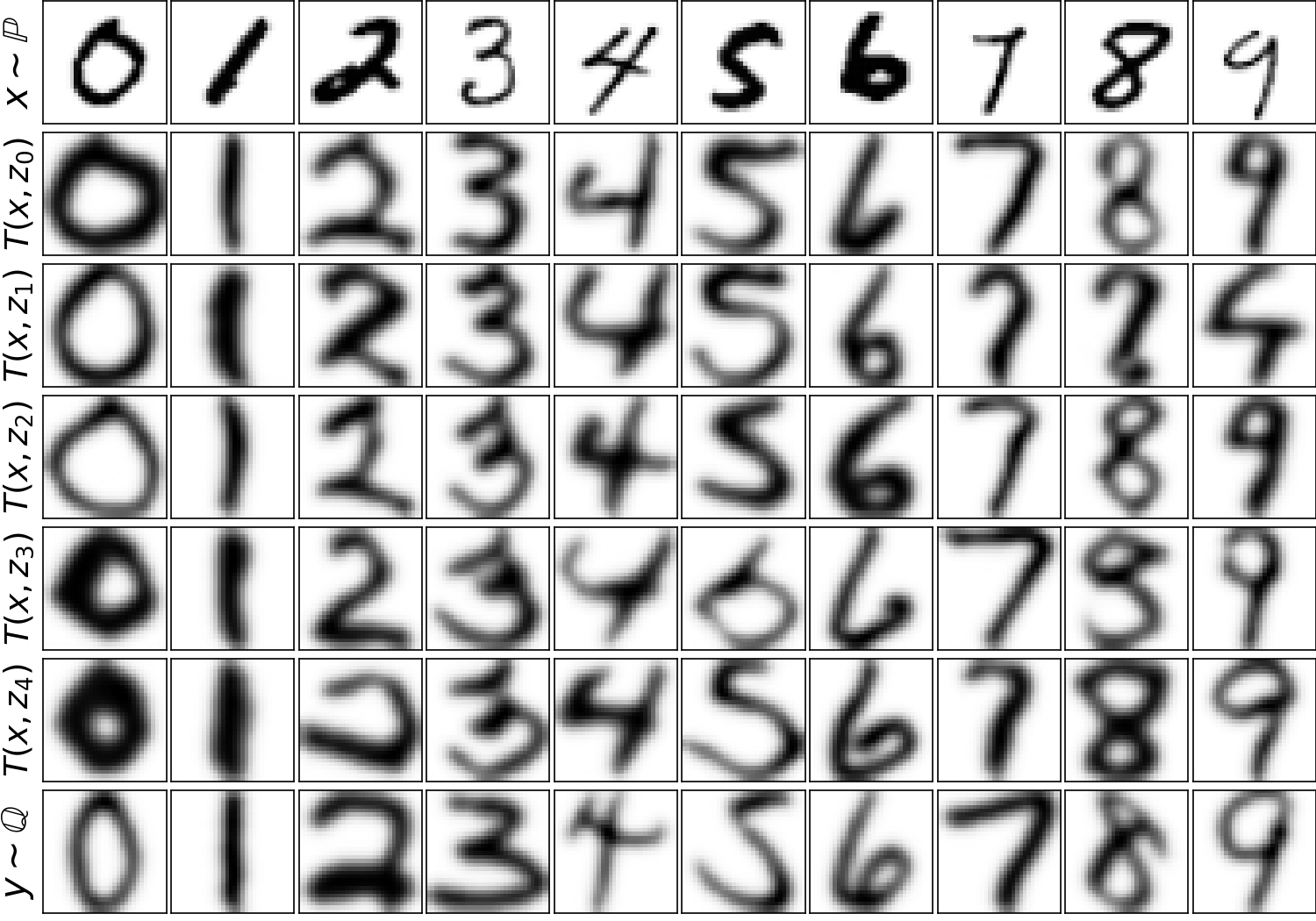
(a) MNIST $\rightarrow$ USPS

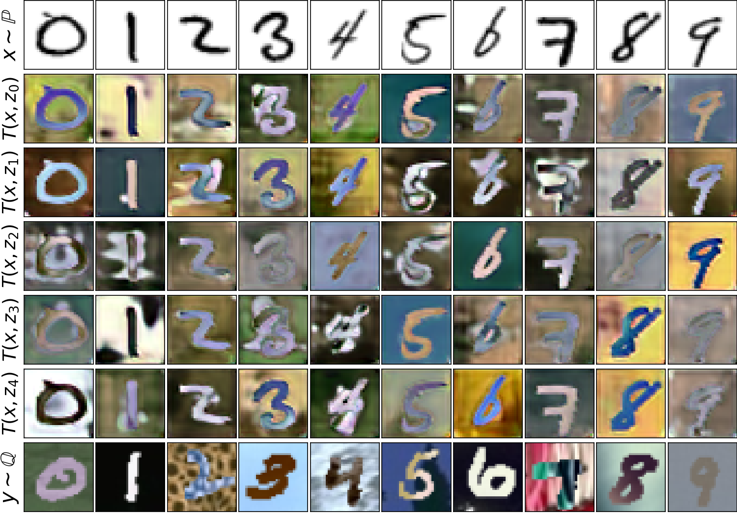
(b) MNIST $\rightarrow$ MNIST-M

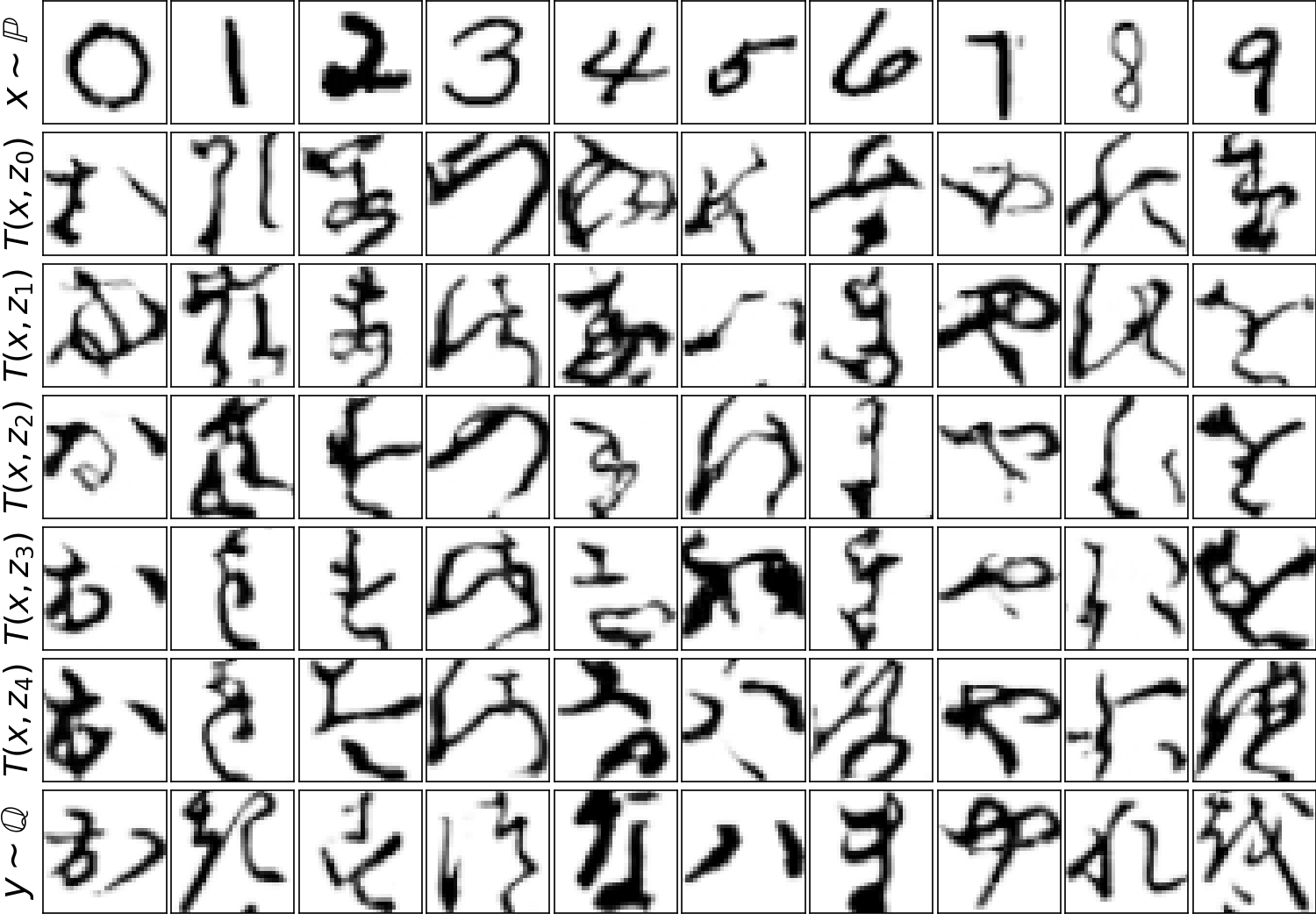
(c) MNIST $\rightarrow$ KMNIST

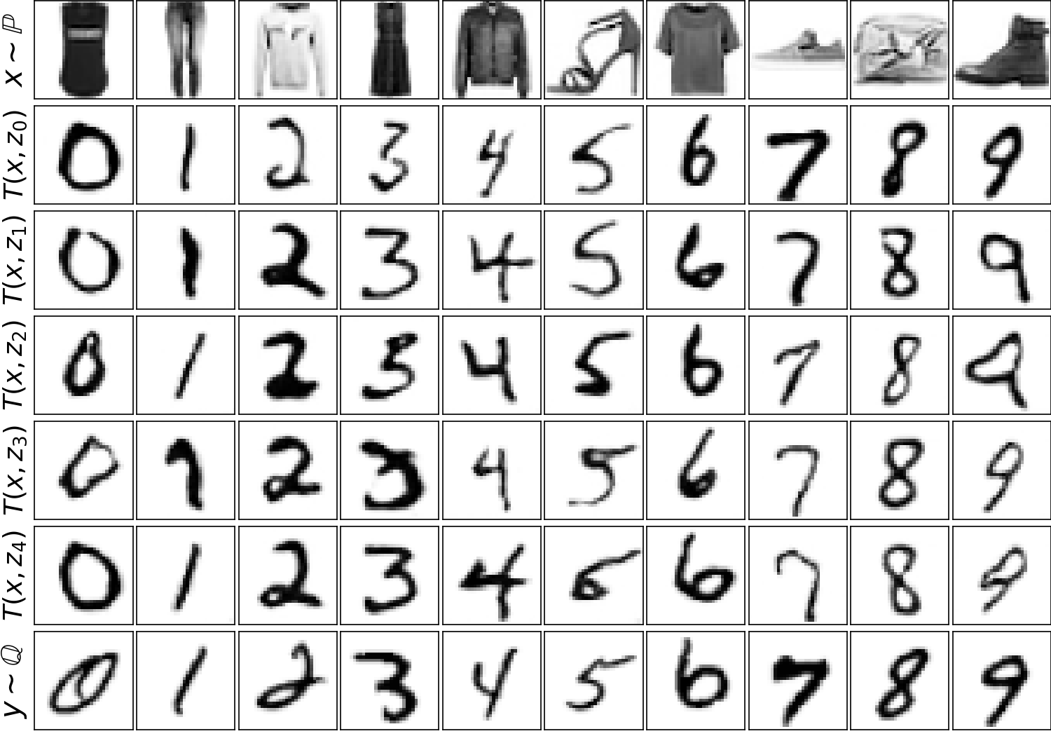
(d) FMNIST $\rightarrow$ MNIST

Figure 7: Stochastic transport maps $T_{\theta}(x,z)$ learned by our Algorithm 1. Additional examples.

C.5 Ablation Study of the Latent Space Dimension

In this subsection, we study the structure of the learned stochastic map for $\mathcal{F}_{\text{G}}$ with different latent space dimensions $Z$. We consider MNIST $\rightarrow$ USPS transfer task (10 classes). The results are shown in Figures 8, 9 and Table 5. As can be seen, our model performs comparably for different $Z$.

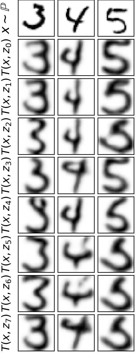
(a) $Z=1$

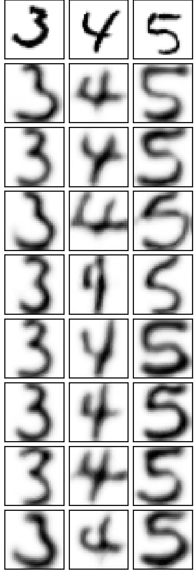
(b) $Z=4$

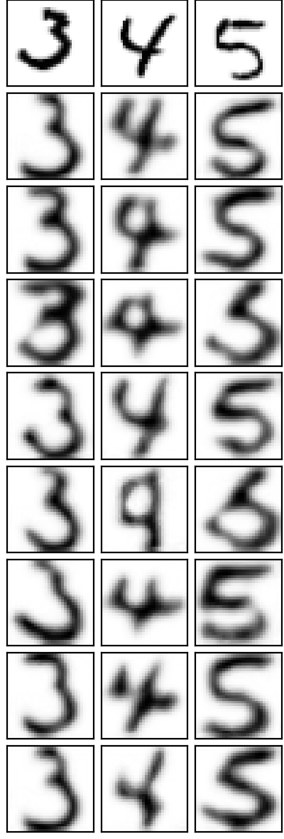
(c) $Z=8$

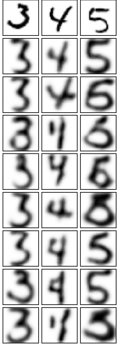
(d) $Z=16$

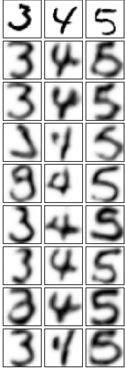
(e) $Z=32$

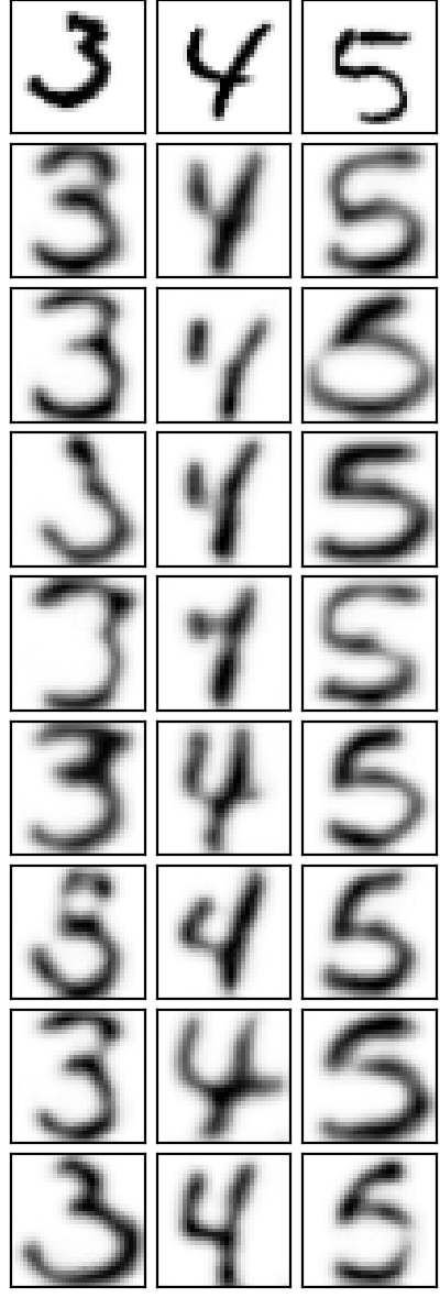
(f) $Z=64$

Figure 8: MNIST $\rightarrow$ USPS translation with functional $\mathcal{F}_{\text{G}}$ and varying $Z=1,4,8,16,32,64$.

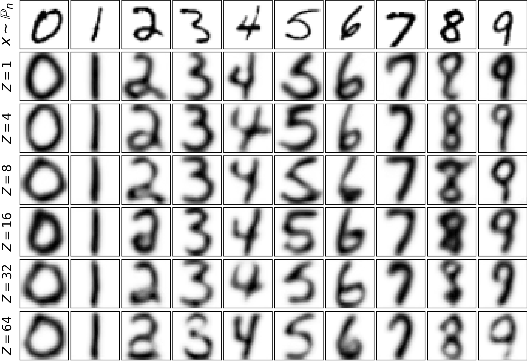
Figure 9: Stochastic transport maps $T_{\theta}(x,z)$ learned by our Algorithm 1 with different sizes of $Z$.

Metrics	$Z=1$	$Z=4$	$Z=8$	$Z=16$	$Z=32$	$Z=64$
Accuracy	86.96	93.48	91.82	92.08	92.25	92.95
FID	4.90	5.88	4.63	3.80	4.34	4.61

Table 5: Accuracy$\uparrow$ and FID$\downarrow$ of the stochastic maps MNIST $\rightarrow$ USPS learned by our translation method with different noise size $Z$.

C.6 Imbalanced Classes

In this subsection, we study the behaviour of the optimal map for $\mathcal{F}_{\text{G}}$ when the classes are imbalanced in input and target domains. Since our method learns a transport map from $\mathbb{P}$ to $\mathbb{Q}$, it should capture the class balance of the $\mathbb{Q}$ regardless of the class balance in $\mathbb{P}$. We check this below.

We consider MNIST $\rightarrow$ USPS datasets with $n=3$ classes in MNIST and $n=3$ classes in USPS. We assume that the class probabilities are $\alpha_{1}=\alpha_{2}=\frac{1}{2}$, $\alpha_{3}=0$ and $\beta_{1}=\beta_{2}=\beta_{3}=\frac{1}{3}$. That is, there is no class $3$ in the source dataset and it is not used anywhere during training. In turn, the target class $3$ is not used when training $T_{\theta}$ but is used when training $f_{\omega}$. All the hyperparameters here are the same as in the previous MNIST $\rightarrow$ USPS experiments with 10 known labels in target classes. The results are shown in Figure 10(a) and 11(a). We present deterministic (no $z$) and stochastic (with $z$) maps.

Our cost functional $\mathcal{F}_{\text{G}}$ stimulates the map to maximally preserve the input class. However, to transport $\mathbb{P}$ to $\mathbb{Q}$, the model must change the class balance. We show the confusion matrix for learned maps $T_{\theta}$ in Figures 10(b), 11(b). It illustrates that the model maximally preserves the input classes $0,1$ and uniformly distributes the input classes 0 and 1 into class 2, as suggested by our cost functional.

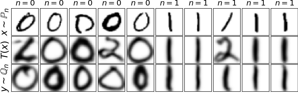
(a) Examples of transported digits $x\mapsto T_{\theta}(x)$.

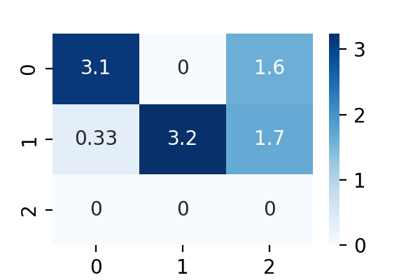
(b) Confusion matrix of $T_{\theta}(x)$.

Figure 10: Imbalanced MNIST $\rightarrow$ USPS translation with functional $\mathcal{F}_{\text{G}}$ (deterministic, no $z$).

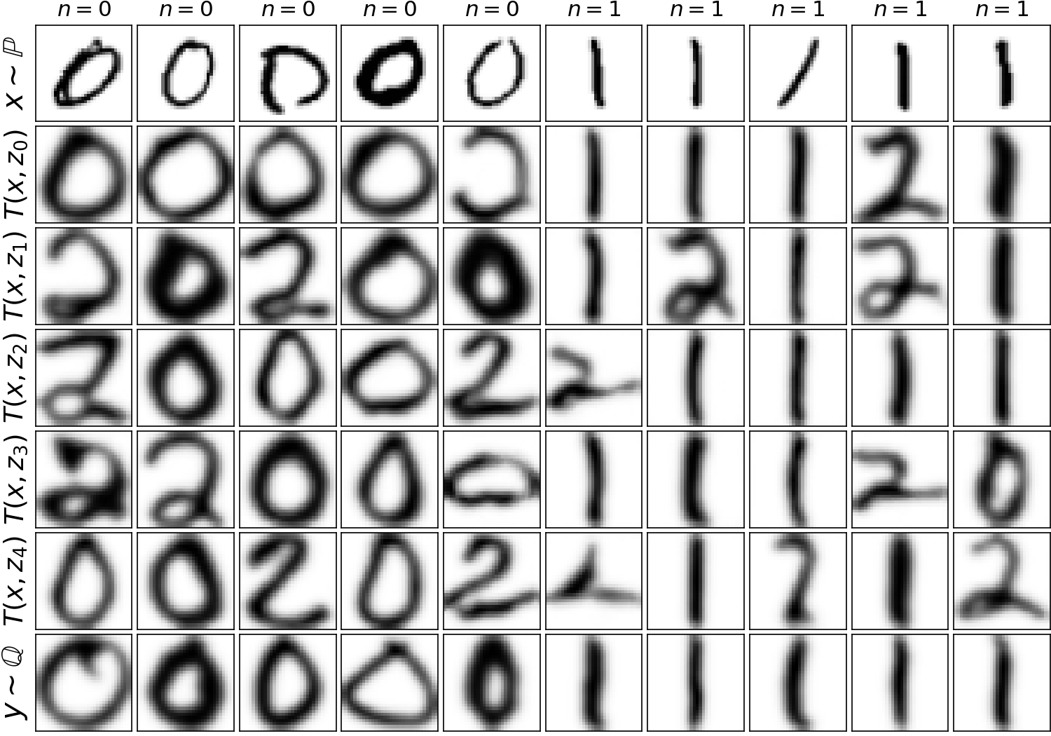
(a) Examples of transported digits $x\mapsto T_{\theta}(x,z)$, $z\sim\mathbb{S}$.

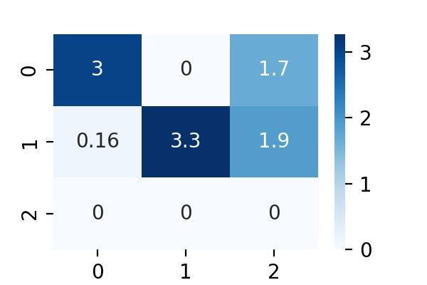
(b) Confusion matrix of $T_{\theta}(x,z)$.

Figure 11: Imbalanced MNIST $\rightarrow$ USPS translation with functional $\mathcal{F}_{\text{G}}$ (stochastic, with $z$).

C.7 ICNN-based dataset transfer

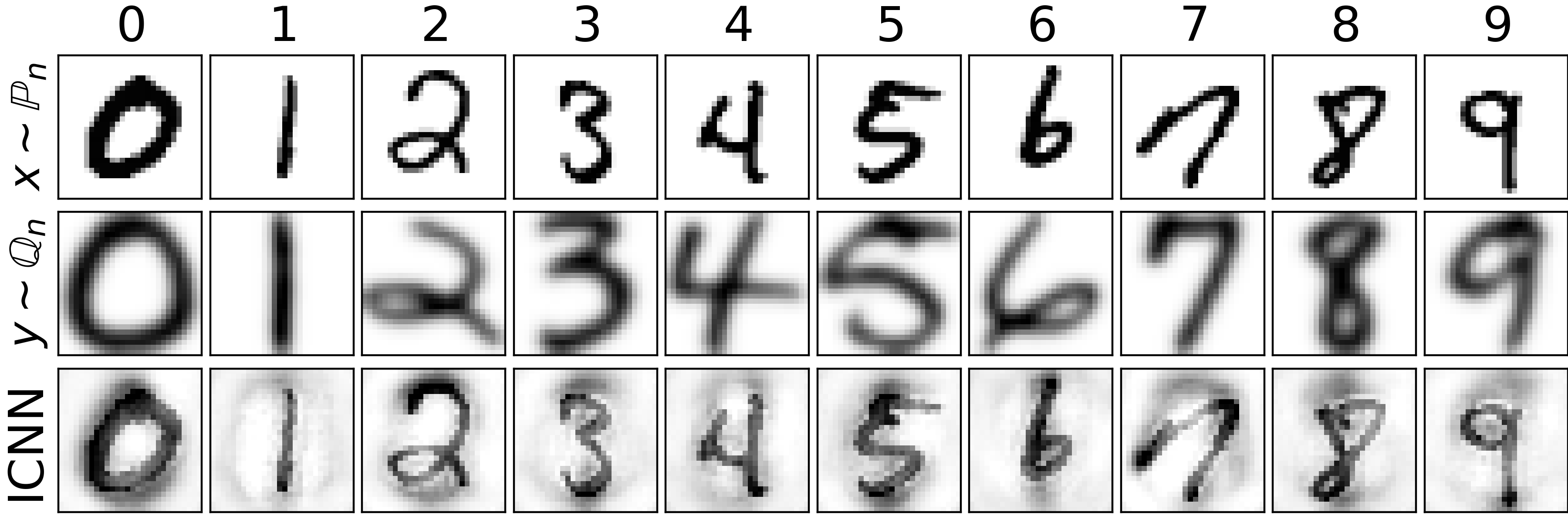
(a) MNIST$\rightarrow$USPS transfer.

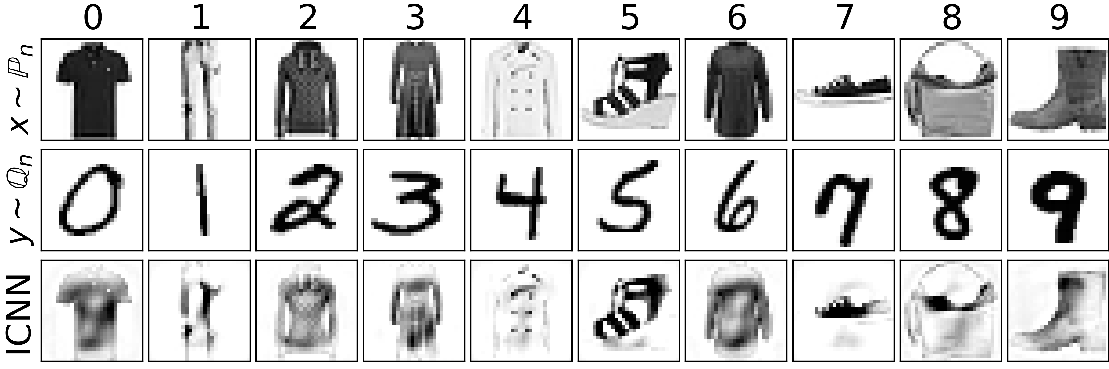
(b) FMNIST$\rightarrow$MNIST transfer.

Figure 12: Results of ICNN-based method applied to the dataset transfer task.

For completeness, we show the performance of ICNN-based method for the classic (1) quadratic transport cost $c(x,y)=\frac{1}{2}\|x-y\|^{2}$ on the dataset transfer task. We use the non-minimax version (Korotin et al., 2021a) of the ICNN-based method by (Makkuva et al., 2020). We employ the publicly available code and dense ICNN architectures from the Wasserstein-2 benchmark repository . The batch size is $K_{B}=32$, the total number of iterations is 100k, $lr=3\cdot 10^{-3}$, and the Adam optimizer is used. The datasets are preprocessed as in the other experiments, see Appendix C.1.

The qualitative results for MNIST$\rightarrow$USPS and FashionMNIST$\rightarrow$MNIST transfer are given in Figure 12. The results are reasonable in the first case (related domains). However, they are visually unpleasant in the second case (unrelated domains). This is expected as the second case is notably harder. More generally, as derived in the Wasserstein-2 benchmark (Korotin et al., 2021b), the ICNN models do not work well in the pixel space due to the poor expressiveness of ICNN architectures. The ICNN method achieved 18.8% accuracy and $\gg$100 FID in the FMNIST$\rightarrow$MNIST transfer, and 35.6% and accuracy and 13.9 FID in the MNIST$\rightarrow$USPS case. All the metrics are much worse than those achieved by our general OT method with the class-guided functional $\mathcal{F}_{G}$, see Table 1, 2 for comparison.

C.8 Non-default class correspondence

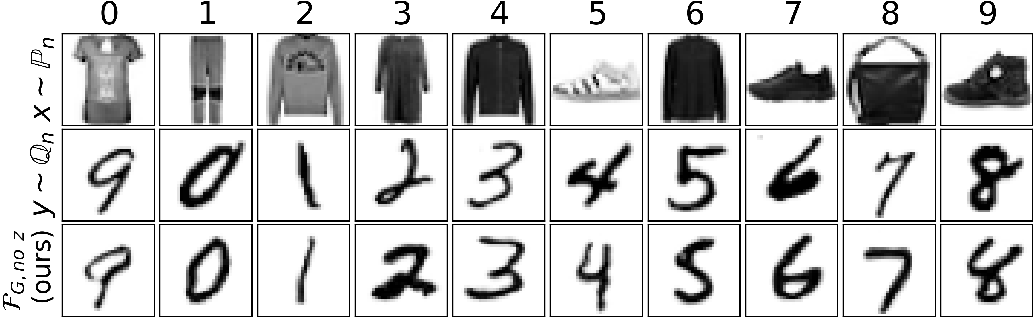
Figure 13: FMNIST$\rightarrow$MNIST mapping with $\mathcal{F}_{G}$ no $z$ cost, classes are permuted.

To show that our method can work with any arbitrary correspondence between datasets, we also consider FMNIST$\rightarrow$MNIST dataset transfer with the following non-default correspondence between the dataset classes:

$$0\mathrel{\hbox{\rule[-0.2pt]{3.0pt}{0.4pt}}\mkern-4.0mu\hbox{\char 41\relax}}9,1\mathrel{\hbox{\rule[-0.2pt]{3.0pt}{0.4pt}}\mkern-4.0mu\hbox{\char 41\relax}}0,2\mathrel{\hbox{\rule[-0.2pt]{3.0pt}{0.4pt}}\mkern-4.0mu\hbox{\char 41\relax}}1,3\mathrel{\hbox{\rule[-0.2pt]{3.0pt}{0.4pt}}\mkern-4.0mu\hbox{\char 41\relax}}2,4\mathrel{\hbox{\rule[-0.2pt]{3.0pt}{0.4pt}}\mkern-4.0mu\hbox{\char 41\relax}}3,5\mathrel{\hbox{\rule[-0.2pt]{3.0pt}{0.4pt}}\mkern-4.0mu\hbox{\char 41\relax}}4,6\mathrel{\hbox{\rule[-0.2pt]{3.0pt}{0.4pt}}\mkern-4.0mu\hbox{\char 41\relax}}5,7\mathrel{\hbox{\rule[-0.2pt]{3.0pt}{0.4pt}}\mkern-4.0mu\hbox{\char 41\relax}}6,8\mathrel{\hbox{\rule[-0.2pt]{3.0pt}{0.4pt}}\mkern-4.0mu\hbox{\char 41\relax}}7,9\mathrel{\hbox{\rule[-0.2pt]{3.0pt}{0.4pt}}\mkern-4.0mu\hbox{\char 41\relax}}8.$$

In this experiment, we use the same architectures and data preprocessing as in dataset transfer tasks; see Appendix C.1. We use our $\mathcal{F}_{G}$ (12) as the cost functional and learn a deterministic transport map $T$ (no $z$). In this setting, our method produces comparable results to the previously reported in Section 5 accuracy equal to 83.1, and FID 6.69. The qualitative results are given in Figure 13.

C.9 Solving batch effect

The batch effect is a well-known issue in biology, particularly in high-throughput genomic studies such as gene expression microarrays, RNA-seq, and proteomics Leek et al. (2010). It occurs when non-biological factors, such as different processing times or laboratory conditions, introduce systematic variations in the data. Addressing batch effects is crucial for ensuring robust and reproducible findings in biological research Lazar et al. (2013). By solving this problem using our method, directly in the input space, we can preserve the samples’ intrinsic structure, minimizing artifacts, and ensuring biological validation.

In our experiments, we map classes across two domains: TM-baron-mouse-for-segerstolpe and segerstolpe-human, consisting of 3,329 and 2,108 samples, respectively. The data was generated by the Splatter package Zappia et al. (2017). Each domain consists of eight classes. The source domain $\mathbb{P}$ is fully-labelled, and the target $\mathbb{Q}$ contains 10 labelled samples per class. Each sample is a 657-sized vector pre-processed with default Splatter settings. Zappia et al. (2017).

We employed feed-forward networks with one hidden layer of size 512 for the map $T_{\theta}$ and a hidden layer of size 1024 for the potential network $v_{\omega}$. To evaluate the accuracy, we trained single-layer neural network classifiers with soft-max output activation, using the available target data. Our method improved accuracy from 63.0 $\rightarrow$ 92.5. Meanwhile, the best DOT solver (EMD) identified through search, as described in Appendix C.1, reduced accuracy from 63.0 $\rightarrow$ 50.4.

Appendix D General functionals with conditional interaction energy regularizer

Generally speaking, for practically useful general cost functionals $\mathcal{F}:\mathcal{M}(\mathcal{X}\times\mathcal{Y})\rightarrow\mathbb{R}\cup\{+\infty\}$ it may be difficult or even impossible to establish their strict or strong convexity. For instance, our considered class-guided functional $\mathcal{F}_{\text{G}}$ (12) is not necessarily strictly convex. In such cases, our results on the uniqueness of OT plan $\pi^{*}$ (Corollary 1) and the closeness of approximate OT plan $\hat{\pi}$ to the true one (Theorem 3) are not directly applicable.

In this section, we propose a generic way to overcome this problem by means of strongly convex regularizers. Let $\mathcal{F},\mathcal{R}:\mathcal{M}(\mathcal{X}\times\mathcal{Y})\rightarrow\mathbb{R}\cup\{+\infty\}$ be convex, lower semi-continuous functionals, which are equal to $+\infty$ on $\mu\in\mathcal{M}(\mathcal{X}\times\mathcal{Y})\setminus\mathcal{P}(\mathcal{X}\times\mathcal{Y})$. Additionally, we will assume that $\mathcal{R}$ is $\beta$-strongly convex on $\Pi(\mathbb{P})$ in some metric $\rho(\cdot,\cdot)$. For $\gamma>0$, one may consider the following $\mathcal{R}$-regularized general OT problem:

$$\inf\limits_{\pi\in\Pi(\mathbb{P},\mathbb{Q})}\big{\{}\mathcal{F}(\pi)+\gamma\mathcal{R}(\pi)\big{\}}.$$

Note that $\pi\mapsto\mathcal{F}(\pi)+\gamma\mathcal{R}(\pi)$ is convex, lower semi-continuous, separately *-increasing (since it equals $+\infty$ outside $\pi\in\mathcal{P}(\mathcal{X}\times\mathcal{Y})$, see the proof of Theorem 4 in Appendix A) and $\beta\gamma$-strongly convex on $\Pi(\mathbb{P})$ in $\rho(\cdot,\cdot)$. In the considered setup, functional $\mathcal{F}$ corresponds to a real problem a practitioner may want to solve, and functional $\mathcal{R}$ is the regularizer which slightly shifts the resulting solution but induces nice theoretical properties. Our proposed technique resembles the idea of the Neural Optimal Transport with Kernel Variance (Korotin et al., 2023a). In this section, we generalize their approach and make it applicable to our duality gap analysis (Theorem 3). Below we introduce an example of a strongly convex regularizer. Corresponding practical demonstrations are left to Appendix D.1.

Conditional interaction energy functional. Let $(\mathcal{Y},l)$ be a semimetric space of negative type (Sejdinovic et al., 2013, §2.1), i.e. $l:\mathcal{Y}\times\mathcal{Y}\rightarrow\mathbb{R}$ is the semimetric and $\forall N\geq 2\,,\,y_{1},y_{2},\dots,y_{N}\in\mathcal{Y}$ and $\forall\alpha_{1},,\alpha_{2},\dots\alpha_{N}\in\mathbb{R}$ such that $\sum_{n=1}^{N}\alpha_{n}=0$ it holds $\sum_{n=1}^{N}\sum_{n^{\prime}=1}^{N}\alpha_{n}\alpha_{n^{\prime}}l(y_{n},y_{n^{\prime}})\leq 0$. The (square of) energy distance $\mathcal{E}_{l}$ w.r.t. semimetric $l$ between probability distributions $\mathbb{Q}_{1},\mathbb{Q}_{2}\in\mathcal{P}(\mathcal{Y})$ is ((Sejdinovic et al., 2013, §2.2)):

$$\mathcal{E}_{l}^{2}(\mathbb{Q}_{1},\mathbb{Q}_{2})=2\mathbb{E}l(Y_{1},Y_{2})-\mathbb{E}l(Y_{1},Y^{\prime}_{1})-\mathbb{E}l(Y_{2},Y^{\prime}_{2}),$$ (37)

where $Y_{1},Y^{\prime}_{1}\sim\mathbb{Q}_{1}$; $Y_{2},Y^{\prime}_{2}\sim\mathbb{Q}_{2}$. Note that for $l(y,y^{\prime})=\frac{1}{2}\|y-y^{\prime}\|_{2}$ formula (37) reduces to (13). The energy distance is known to be a metric on $\mathcal{P}(\mathcal{Y})$ (Klebanov et al., 2005) (note that $\mathcal{Y}$ is compact). The examples of semimetrics of negative type include $l(y,y^{\prime})=\|x-y\|_{p}^{\min\{1,p\}}$ for $0<p\leq 2$ (Meckes, 2013, Th. 3.6).

Consider the following generalization of energy distance $\mathcal{E}_{l}$ on space $\Pi(\mathbb{P})$. Let $\pi_{1},\pi_{2}\in\Pi(\mathbb{P})$.

$$\rho_{l}^{2}(\pi_{1},\pi_{2})\stackrel{{\scriptstyle\text{def}}}{{=}}\int_{\mathcal{X}}\mathcal{E}_{l}^{2}(\pi_{1}(\cdot|x),\pi_{2}(\cdot|x))d\mathbb{P}(x).$$ (38)

Proposition 2.

It holds that $\rho_{l}(\cdot,\cdot)$ is a metric on $\Pi(\mathbb{P})$.

Proof of Proposition 2.

Obviously, $\forall\pi\in\Pi(\mathbb{P}):\rho_{l}(\pi,\pi)=0$ and $\forall\pi_{1},\pi_{2}\in\Pi(\mathbb{P}):\rho_{l}(\pi_{1},\pi_{2})=\rho_{l}(\pi_{2},\pi_{1})\geq 0$. We are left to check the triangle inequality. Consider $\pi_{1},\pi_{2},\pi_{3}\in\Pi(\mathbb{P})$. In what follows, for $\pi\in\Pi(\mathbb{P})$ and $x\in\mathcal{X}$, we denote the conditional distribution $\pi(\cdot|x)$ as $\pi^{x}$:

$$\rho_{l}(\pi_{1},\pi_{2})+\rho_{l}(\pi_{2},\pi_{3})\geq\rho_{l}(\pi_{1},\pi_{3})\Leftrightarrow$$

$$(\rho_{l}(\pi_{1},\pi_{2})+\rho_{l}(\pi_{2},\pi_{3}))^{2}\geq\rho_{l}^{2}(\pi_{1},\pi_{3})\Leftrightarrow$$

$$\!\!\!\!\!\!\!\!\!\!\!\!\int_{\mathcal{X}}\!\!\!\!\mathcal{E}_{l}^{2}(\pi_{1}^{x},\pi_{2}^{x})d\mathbb{P}(x)\!+\!\!\int_{\mathcal{X}}\!\!\!\!\mathcal{E}_{l}^{2}(\pi_{2}^{x},\pi_{3}^{x})d\mathbb{P}(x)\!+\!2\sqrt{\!\!\int_{\mathcal{X}}\!\!\!\!\mathcal{E}_{l}^{2}(\pi_{1}^{x},\pi_{2}^{x})d\mathbb{P}(x)\!\!\int_{\mathcal{X}}\!\!\!\!\mathcal{E}_{l}^{2}(\pi_{2}^{x},\pi_{3}^{x})d\mathbb{P}(x)}\!\geq\!\!\int_{\mathcal{X}}\!\!\!\!\mathcal{E}_{l}^{2}(\pi_{1}^{x},\pi_{3}^{x})d\mathbb{P}(x)\Leftarrow$$ (39)

$$\int_{\mathcal{X}}\!\!\mathcal{E}_{l}^{2}(\pi_{1}^{x},\pi_{2}^{x})d\mathbb{P}(x)\!+\!\int_{\mathcal{X}}\!\!\mathcal{E}_{l}^{2}(\pi_{2}^{x},\pi_{3}^{x})d\mathbb{P}(x)\!+2\!\int_{\mathcal{X}}\!\!\mathcal{E}_{l}(\pi_{1}^{x},\pi_{2}^{x})\mathcal{E}_{l}(\pi_{2}^{x},\pi_{3}^{x})d\mathbb{P}(x)\!\geq\!\int_{\mathcal{X}}\!\!\mathcal{E}_{l}^{2}(\pi_{1}^{x},\pi_{3}^{x})d\mathbb{P}(x)\Leftrightarrow$$

$$\int_{\mathcal{X}}\underbrace{\big{[}(\mathcal{E}_{l}(\pi_{1}^{x},\pi_{2}^{x})+\mathcal{E}_{l}(\pi_{2}^{x},\pi_{3}^{x}))^{2}-\mathcal{E}_{l}^{2}(\pi_{1}^{x},\pi_{3}^{x})\big{]}}_{\geq 0\text{ due to triangle inequality for }\mathcal{E}_{l}}d\mathbb{P}(x)\geq 0,$$

where in line (39) we apply the Cauchy–Bunyakovsky inequality (Bouniakowsky, 1859):

$$\int_{\mathcal{X}}\!\!\mathcal{E}_{l}^{2}(\pi_{1}^{x},\pi_{2}^{x})d\mathbb{P}(x)\!\!\int_{\mathcal{X}}\!\!\mathcal{E}_{l}^{2}(\pi_{2}^{x},\pi_{3}^{x})d\mathbb{P}(x)\geq\left(\int_{\mathcal{X}}\mathcal{E}_{l}(\pi_{1}^{x},\pi_{2}^{x})\mathcal{E}_{l}(\pi_{2}^{x},\pi_{3}^{x})d\mathbb{P}(x)\right)^{2}.$$

∎

Now we are ready to introduce our proposed strongly convex (w.r.t. $\rho_{l}$) regularizer. Let $\pi\in\Pi(\mathcal{X})$ and $l$ be a semimetric on $\mathcal{Y}$ of negative type. We define

$$\mathcal{R}_{l}(\pi)=-\frac{1}{2}\int_{\mathcal{X}}\int_{\mathcal{Y}}\int_{\mathcal{Y}}l(y,y^{\prime})d\pi^{x}(y)d\pi^{x}(y^{\prime})d\mathbb{P}(x).$$ (40)

We call $\mathcal{R}_{l}$ to be conditional interaction energy functional. In the context of solving the OT problem, it was first introduced in (Korotin et al., 2023a) from the perspectives of RKHS and kernel embeddings (Sejdinovic et al., 2013, §3). The authors of (Korotin et al., 2023a) establish the conditions under which the semi-dual (max-min) formulation of weak OT problem regularized with $\mathcal{R}_{l}$ yields the unique solution, i.e., they deal with the strict convexity of $\mathcal{R}_{l}$. In contrast, our paper exploits strong convexity and provides the additional error analysis (Theorem 3) which helps with tailoring theoretical guarantees to actual practical procedures for arbitrary strongly convex functionals. Below, we prove that $\mathcal{R}_{l}$ is strongly convex w.r.t. $\rho_{l}$ and, under additional assumptions on $l$, is lower semi-continuous.

Proposition 3.

$\mathcal{R}_{l}$ is $1$-strongly convex on $\Pi(\mathbb{P})$ w.r.t. $\rho_{l}$.

Proof of Proposition 3.

Let $\pi_{1},\pi_{2}\in\Pi(\mathbb{P})$, $0\leq\alpha\leq 1$. Consider the left-hand side of (23):

$$\mathcal{R}_{l}(\alpha\pi_{1}+(1-\alpha)\pi_{2})=$$

$$-\frac{1}{2}\int_{\mathcal{X}}\int_{\mathcal{Y}\times\mathcal{Y}}\!\!\!\!l(y,y^{\prime})d[\alpha\pi_{1}+(1-\alpha)\pi_{2}]^{x}(y)d[\alpha\pi_{1}+(1-\alpha)\pi_{2}]^{x}(y^{\prime})d\mathbb{P}(x)=$$

$$-\frac{1}{2}\alpha^{2}\int_{\mathcal{X}}\int_{\mathcal{Y}\times\mathcal{Y}}\!\!\!\!l(y,y^{\prime})d\pi_{1}^{x}(y)d\pi_{1}^{x}(y^{\prime})d\mathbb{P}(x)+\quad\,\,$$

$$-\alpha(1-\alpha)\int_{\mathcal{X}}\int_{\mathcal{Y}\times\mathcal{Y}}\!\!\!\!l(y,y^{\prime})d\pi_{1}^{x}(y)d\pi_{2}^{x}(y^{\prime})d\mathbb{P}(x)+\quad\,\,$$

$$-\frac{1}{2}(1-\alpha)^{2}\int_{\mathcal{X}}\int_{\mathcal{Y}\times\mathcal{Y}}\!\!\!\!l(y,y^{\prime})d\pi_{2}^{x}(y)d\pi_{2}^{x}(y^{\prime})d\mathbb{P}(x)=$$

$$\bigg{(}-\frac{1}{2}\alpha+\frac{1}{2}\alpha(1-\alpha)\bigg{)}\int_{\mathcal{X}}\int_{\mathcal{Y}\times\mathcal{Y}}\!\!\!\!l(y,y^{\prime})d\pi_{1}^{x}(y)d\pi_{1}^{x}(y^{\prime})d\mathbb{P}(x)+\quad\,\,$$

$$-\alpha(1-\alpha)\int_{\mathcal{X}}\int_{\mathcal{Y}\times\mathcal{Y}}\!\!\!\!l(y,y^{\prime})d\pi_{1}^{x}(y)d\pi_{2}^{x}(y^{\prime})d\mathbb{P}(x)+\quad\,\,$$

$$\bigg{(}-\frac{1}{2}(1-\alpha)+\frac{1}{2}\alpha(1-\alpha)\bigg{)}\int_{\mathcal{X}}\int_{\mathcal{Y}\times\mathcal{Y}}\!\!\!\!l(y,y^{\prime})d\pi_{2}^{x}(y)d\pi_{2}^{x}(y^{\prime})d\mathbb{P}(x)=$$

$$\underbrace{-\frac{1}{2}\alpha\!\!\int_{\mathcal{X}}\!\int_{\mathcal{Y}\times\mathcal{Y}}\!\!\!\!l(y,y^{\prime})d\pi_{1}^{x}(y)d\pi_{1}^{x}(y^{\prime})d\mathbb{P}(x)}_{=\alpha\mathcal{R}_{l}(\pi_{1})}\underbrace{-\frac{1}{2}(1-\alpha)\!\!\int_{\mathcal{X}}\!\int_{\mathcal{Y}\times\mathcal{Y}}\!\!\!\!l(y,y^{\prime})d\pi_{2}^{x}(y)d\pi_{2}^{x}(y^{\prime})d\mathbb{P}(x)}_{=(1-\alpha)\mathcal{R}_{l}(\pi_{2})}+\quad\,\,$$

$$\!\!\!\!\!\!\!\!\frac{\alpha(1\!-\!\alpha)}{2}\!\!\int_{\mathcal{X}}\underbrace{\!\!\bigg{(}\!\int_{\mathcal{Y}\times\mathcal{Y}}\!\!\!\!\!\!\!\!l(y,y^{\prime})d\pi_{1}^{x}(y)d\pi_{1}^{x}(y^{\prime})\!+\!\!\int_{\mathcal{Y}\times\mathcal{Y}}\!\!\!\!\!\!\!\!l(y,y^{\prime})d\pi_{2}^{x}(y)d\pi_{2}^{x}(y^{\prime})\!-\!2\!\int_{\mathcal{Y}\times\mathcal{Y}}\!\!\!\!\!\!\!\!l(y,y^{\prime})d\pi_{1}^{x}(y)d\pi_{2}^{x}(y^{\prime})\!\!\bigg{)}}_{=-\mathcal{E}_{l}(\pi_{1}^{x},\pi_{2}^{x})}d\mathbb{P}(x)=$$

$$\alpha\mathcal{R}_{l}(\pi_{1})+(1-\alpha)\mathcal{R}_{l}(\pi_{2})-\frac{1}{2}\alpha(1-\alpha)\rho_{l}^{2}(\pi_{1},\pi_{2}),$$

i.e., $\mathcal{R}_{l}(\alpha\pi_{1}\!+\!(1\!-\!\alpha)\pi_{2})\!=\!\alpha\mathcal{R}_{l}(\pi_{1})\!+\!(1\!-\!\alpha)\mathcal{R}_{l}(\pi_{2})-\frac{\alpha(1-\alpha)}{2}\rho_{l}^{2}(\pi_{1},\pi_{2})$, which finishes the proof. ∎

Proposition 4.

Assume that $l$ is continuous (it is the case for all reasonable semimetrics $l$). Then $\mathcal{R}_{l}$ is lower semi-continuous on $\Pi(\mathbb{P})$.

Proof of Proposition 4.

Consider the functional $\mathcal{W}_{l}:\mathcal{X}\times\mathcal{P}(\mathcal{Y})\rightarrow\mathbb{R}\cup\{+\infty\}$:

$$\mathcal{W}_{l}(x,\mu)=-\int_{\mathcal{Y}\times\mathcal{Y}}l(y,y^{\prime})d\mu(y)d\mu(y^{\prime}),$$

then the conditional interaction energy functional could be expressed as follows: $\mathcal{R}_{l}(\pi)=\frac{1}{2}\int_{\mathcal{X}}\mathcal{W}_{l}(x,\pi^{x})d\mathbb{P}(x)$. We are to check that $\mathcal{W}_{l}$ satisfies Condition (A+) in (Backhoff-Veraguas et al., 2019, Definition 2.7). Note that $\mathcal{W}_{l}$ actually does not depend on $x\in\mathcal{X}$.

• The lower-semicontinuity of $\mathcal{W}_{l}$ follows from (Santambrogio, 2015, Proposition 7.2) and the equivalence of the weak convergence and the convergence w.r.t. Wasserstein metric on $\mathcal{P}(\mathcal{Y})$ where $\mathcal{Y}$ is compact, see (Villani, 2008, Theorem 6.8).

• Since $(y,y^{\prime})\mapsto-l(y,y^{\prime})$ is a lower-semicontinuous, it achieves its minimum on the compact $\mathcal{Y}\times\mathcal{Y}$ which lower-bounds the functional $\mathcal{W}_{l}$.

• The convexity (even 1-strong convexity w.r.t. metric $\mathcal{E}_{l}(\cdot,\cdot)$) of functional $\mathcal{W}_{l}$ was de facto established in Proposition 3. In particular, given $\mu_{1},\mu_{2}\in\mathcal{P}(\mathcal{Y})$, $\alpha\in(0,1)$, $x\in\mathcal{X}$ it holds:

  $$\mathcal{W}_{l}(x,\alpha\mu_{1}\!+\!(1\!-\!\alpha)\mu_{2})\!=\!\alpha\mathcal{W}_{l}(x,\mu_{1})\!+\!(1\!-\!\alpha)\mathcal{W}_{l}(x,\mu_{2})-\frac{\alpha(1-\alpha)}{2}\mathcal{E}_{l}^{2}(\mu_{1},\mu_{2}).$$

The application of (Backhoff-Veraguas et al., 2019, Proposition 2.8, Eq. (2.16)) finishes the proof. ∎

D.1 Experiments with conditional interaction energy regularizer

In the previous Section D, we introduce an example of the strongly convex regularizer. In this section, we present experiments to investigate the impact of strongly convex regularization on our general cost functional $\mathcal{F}_{\text{G}}$. In particular, we conduct experiments on the FMNIST-MNIST dataset transfer problem using the proposed conditional interaction energy regularizer with $l(y,y^{\prime})=\|y-y^{\prime}\|_{2}$. To empirically estimate the impact of the regularization, we test different coefficients $\gamma\in[0.001,0.01,0.1]$. The results are shown in the following Figure LABEL:tab:kernel and Table 14.

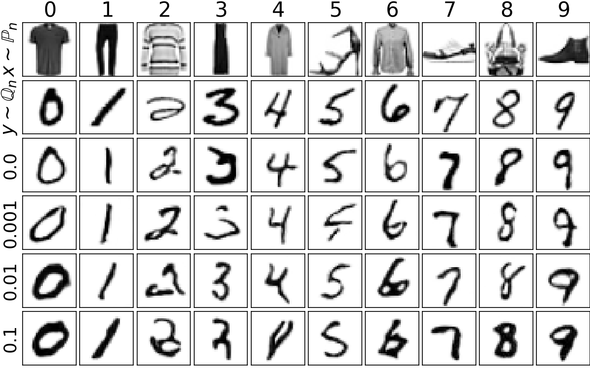
Figure 14: Qualitative results of the FMNIST$\rightarrow$MNIST mapping with $\mathcal{F}_{G}$ cost and using different values $\gamma$ of the conditional interaction energy regularization.

$\gamma$	0	0.001	0.01	0.1
Accuracy$\uparrow$	83.33	81.87	79.47	65.11
FID $\downarrow$	5.27	7.67	3.95	7.33

Table 6: Accuracy$\uparrow$ and FID $\downarrow$ of the map learned on FMNIST$\rightarrow$MNIST with $\mathcal{F}_{G}$ cost and different values $\gamma$ of the conditional interaction energy regularization.

It can be seen that the small amount of regularization ($\gamma=0.001$) does not affect the results. But high values decrease the accuracy, which is expected because the regularization contradicts the dataset transfer problem. Increasing the value of $\gamma$ shifts the solution to be more diverse instead of matching the classes.

References

- Alibert et al. (2019) J-J Alibert, Guy Bouchitté, and Thierry Champion. A new class of costs for optimal transport planning. European Journal of Applied Mathematics, 30(6):1229–1263, 2019.
- Almahairi et al. (2018) Amjad Almahairi, Sai Rajeshwar, Alessandro Sordoni, Philip Bachman, and Aaron Courville. Augmented cyclegan: Learning many-to-many mappings from unpaired data. In International Conference on Machine Learning, pp. 195–204. PMLR, 2018.
- Alvarez-Melis & Fusi (2020) David Alvarez-Melis and Nicolo Fusi. Geometric dataset distances via optimal transport. Advances in Neural Information Processing Systems, 33:21428–21439, 2020.
- Alvarez-Melis & Fusi (2021) David Alvarez-Melis and Nicolò Fusi. Dataset dynamics via gradient flows in probability space. In International Conference on Machine Learning, pp. 219–230. PMLR, 2021.
- Alvarez-Melis et al. (2021) David Alvarez-Melis, Yair Schiff, and Youssef Mroueh. Optimizing functionals on the space of probabilities with input convex neural networks. arXiv preprint arXiv:2106.00774, 2021.
- Amos et al. (2017) Brandon Amos, Lei Xu, and J Zico Kolter. Input convex neural networks. In Proceedings of the 34th International Conference on Machine Learning-Volume 70, pp. 146–155. JMLR. org, 2017.
- Arjovsky & Bottou (2017) Martin Arjovsky and Léon Bottou. Towards principled methods for training generative adversarial networks. arXiv preprint arXiv:1701.04862, 2017.
- Backhoff-Veraguas et al. (2019) Julio Backhoff-Veraguas, Mathias Beiglböck, and Gudmun Pammer. Existence, duality, and cyclical monotonicity for weak transport costs. Calculus of Variations and Partial Differential Equations, 58(6):1–28, 2019.
- Bonneel & Digne (2023) Nicolas Bonneel and Julie Digne. A survey of optimal transport for computer graphics and computer vision. In Computer Graphics Forum, 2023.
- Bouniakowsky (1859) Victor Bouniakowsky. Sur quelques inégalités concernant les intégrales ordinaires et les intégrales aux différences finies, volume 1. Mem. Acad. St. Petersburg, 1859.
- Bunne et al. (2021) Charlotte Bunne, Laetitia Meng-Papaxanthos, Andreas Krause, and Marco Cuturi. Jkonet: Proximal optimal transport modeling of population dynamics, 2021.
- Clanuwat et al. (2018) Tarin Clanuwat, Mikel Bober-Irizar, Asanobu Kitamoto, Alex Lamb, Kazuaki Yamamoto, and David Ha. Deep learning for classical japanese literature. arXiv preprint arXiv:1812.01718, 2018.
- Courty et al. (2016) Nicolas Courty, Rémi Flamary, Devis Tuia, and Alain Rakotomamonjy. Optimal transport for domain adaptation. IEEE transactions on pattern analysis and machine intelligence, 39(9):1853–1865, 2016.
- Cuturi (2013) Marco Cuturi. Sinkhorn distances: Lightspeed computation of optimal transport. In Advances in neural information processing systems, pp. 2292–2300, 2013.
- Daniels et al. (2021) Grady Daniels, Tyler Maunu, and Paul Hand. Score-based generative neural networks for large-scale optimal transport. Advances in Neural Information Processing Systems, 34, 2021.
- Deb et al. (2021) Nabarun Deb, Promit Ghosal, and Bodhisattva Sen. Rates of estimation of optimal transport maps using plug-in estimators via barycentric projections. Advances in Neural Information Processing Systems, 34:29736–29753, 2021.
- Essid & Solomon (2018) Montacer Essid and Justin Solomon. Quadratically regularized optimal transport on graphs. SIAM Journal on Scientific Computing, 40(4):A1961–A1986, 2018.
- Fan et al. (2021a) Jiaojiao Fan, Shu Liu, Shaojun Ma, Yongxin Chen, and Haomin Zhou. Scalable computation of monge maps with general costs. arXiv preprint arXiv:2106.03812, 2021a.
- Fan et al. (2021b) Jiaojiao Fan, Amirhossein Taghvaei, and Yongxin Chen. Variational wasserstein gradient flow. arXiv preprint arXiv:2112.02424, 2021b.
- Fan et al. (2023) Jiaojiao Fan, Shu Liu, Shaojun Ma, Hao-Min Zhou, and Yongxin Chen. Neural monge map estimation and its applications. Transactions on Machine Learning Research, 2023. ISSN 2835-8856. URL https://openreview.net/forum?id=2mZSlQscj3. Featured Certification.
- Ferradans et al. (2014) Sira Ferradans, Nicolas Papadakis, Gabriel Peyré, and Jean-François Aujol. Regularized discrete optimal transport. SIAM Journal on Imaging Sciences, 7(3):1853–1882, 2014.
- Flamary et al. (2021) Rémi Flamary, Nicolas Courty, Alexandre Gramfort, Mokhtar Z Alaya, Aurélie Boisbunon, Stanislas Chambon, Laetitia Chapel, Adrien Corenflos, Kilian Fatras, Nemo Fournier, et al. Pot: Python optimal transport. The Journal of Machine Learning Research, 22(1):3571–3578, 2021.
- Ganin & Lempitsky (2015) Yaroslav Ganin and Victor S. Lempitsky. Unsupervised domain adaptation by backpropagation. In Francis R. Bach and David M. Blei (eds.), Proceedings of the 32nd International Conference on Machine Learning, ICML 2015, Lille, France, 6-11 July 2015, volume 37 of JMLR Workshop and Conference Proceedings, pp. 1180–1189. JMLR.org, 2015. URL http://proceedings.mlr.press/v37/ganin15.html.
- Gazdieva et al. (2022) Milena Gazdieva, Litu Rout, Alexander Korotin, Alexander Filippov, and Evgeny Burnaev. Unpaired image super-resolution with optimal transport maps. arXiv preprint arXiv:2202.01116, 2022.
- Genevay (2019) Aude Genevay. Entropy-regularized optimal transport for machine learning. PhD thesis, Paris Sciences et Lettres (ComUE), 2019.
- Genevay et al. (2016) Aude Genevay, Marco Cuturi, Gabriel Peyré, and Francis Bach. Stochastic optimization for large-scale optimal transport. In Advances in neural information processing systems, pp. 3440–3448, 2016.
- Genevay et al. (2019) Aude Genevay, Lénaic Chizat, Francis Bach, Marco Cuturi, and Gabriel Peyré. Sample complexity of sinkhorn divergences. In The 22nd international conference on artificial intelligence and statistics, pp. 1574–1583. PMLR, 2019.
- Gozlan & Juillet (2020) Nathael Gozlan and Nicolas Juillet. On a mixture of brenier and strassen theorems. Proceedings of the London Mathematical Society, 120(3):434–463, 2020.
- Gozlan et al. (2017) Nathael Gozlan, Cyril Roberto, Paul-Marie Samson, and Prasad Tetali. Kantorovich duality for general transport costs and applications. Journal of Functional Analysis, 273(11):3327–3405, 2017.
- Gretton et al. (2012) Arthur Gretton, Karsten M. Borgwardt, Malte J. Rasch, Bernhard Schölkopf, and Alexander J. Smola. A kernel two-sample test. J. Mach. Learn. Res., 13:723–773, 2012. URL http://dl.acm.org/citation.cfm?id=2188410.
- He et al. (2016) Kaiming He, Xiangyu Zhang, Shaoqing Ren, and Jian Sun. Deep residual learning for image recognition. In Proceedings of the IEEE conference on computer vision and pattern recognition, pp. 770–778, 2016.
- Henry-Labordere (2019) Pierre Henry-Labordere. (martingale) optimal transport and anomaly detection with neural networks: A primal-dual algorithm. Available at SSRN 3370910, 2019.
- Heusel et al. (2017) Martin Heusel, Hubert Ramsauer, Thomas Unterthiner, Bernhard Nessler, and Sepp Hochreiter. GANs trained by a two time-scale update rule converge to a local nash equilibrium. In Advances in neural information processing systems, pp. 6626–6637, 2017.
- Hoffman et al. (2018) Judy Hoffman, Eric Tzeng, Taesung Park, Jun-Yan Zhu, Phillip Isola, Kate Saenko, Alexei A. Efros, and Trevor Darrell. Cycada: Cycle-consistent adversarial domain adaptation. In Jennifer G. Dy and Andreas Krause (eds.), Proceedings of the 35th International Conference on Machine Learning, ICML 2018, Stockholmsmässan, Stockholm, Sweden, July 10-15, 2018, volume 80 of Proceedings of Machine Learning Research, pp. 1994–2003. PMLR, 2018. URL http://proceedings.mlr.press/v80/hoffman18a.html.
- Huang et al. (2018) Xun Huang, Ming-Yu Liu, Serge Belongie, and Jan Kautz. Multimodal unsupervised image-to-image translation. In Proceedings of the European conference on computer vision (ECCV), pp. 172–189, 2018.
- Hütter & Rigollet (2021) Jan-Christian Hütter and Philippe Rigollet. Minimax estimation of smooth optimal transport maps. 2021.
- Kingma & Ba (2014) Diederik P Kingma and Jimmy Ba. Adam: A method for stochastic optimization. arXiv preprint arXiv:1412.6980, 2014.
- Klebanov et al. (2005) Lev Borisovich Klebanov, Viktor Beneš, and Ivan Saxl. N-distances and their applications. Charles University in Prague, the Karolinum Press Prague, Czech Republic, 2005.
- Korotin et al. (2021a) Alexander Korotin, Vage Egiazarian, Arip Asadulaev, Alexander Safin, and Evgeny Burnaev. Wasserstein-2 generative networks. In International Conference on Learning Representations, 2021a. URL https://openreview.net/forum?id=bEoxzW_EXsa.
- Korotin et al. (2021b) Alexander Korotin, Lingxiao Li, Aude Genevay, Justin M Solomon, Alexander Filippov, and Evgeny Burnaev. Do neural optimal transport solvers work? a continuous wasserstein-2 benchmark. Advances in Neural Information Processing Systems, 34:14593–14605, 2021b.
- Korotin et al. (2021c) Alexander Korotin, Lingxiao Li, Justin Solomon, and Evgeny Burnaev. Continuous wasserstein-2 barycenter estimation without minimax optimization. In International Conference on Learning Representations, 2021c. URL https://openreview.net/forum?id=3tFAs5E-Pe.
- Korotin et al. (2022a) Alexander Korotin, Vage Egiazarian, Lingxiao Li, and Evgeny Burnaev. Wasserstein iterative networks for barycenter estimation. In Thirty-Sixth Conference on Neural Information Processing Systems, 2022a. URL https://openreview.net/forum?id=GiEnzxTnaMN.
- Korotin et al. (2022b) Alexander Korotin, Alexander Kolesov, and Evgeny Burnaev. Kantorovich strikes back! wasserstein GANs are not optimal transport? In Thirty-sixth Conference on Neural Information Processing Systems Datasets and Benchmarks Track, 2022b. URL https://openreview.net/forum?id=VtEEpi-dGlt.
- Korotin et al. (2023a) Alexander Korotin, Daniil Selikhanovych, and Evgeny Burnaev. Kernel neural optimal transport. In International Conference on Learning Representations, 2023a. URL https://openreview.net/forum?id=Zuc_MHtUma4.
- Korotin et al. (2023b) Alexander Korotin, Daniil Selikhanovych, and Evgeny Burnaev. Neural optimal transport. In International Conference on Learning Representations, 2023b. URL https://openreview.net/forum?id=d8CBRlWNkqH.
- Kouw & Loog (2018) Wouter M Kouw and Marco Loog. An introduction to domain adaptation and transfer learning. arXiv preprint arXiv:1812.11806, 2018.
- Lazar et al. (2013) Cosmin Lazar, Stijn Meganck, Jonatan Taminau, David Steenhoff, Alain Coletta, Colin Molter, David Y Weiss-Solís, Robin Duque, Hugues Bersini, and Ann Nowé. Batch effect removal methods for microarray gene expression data integration: a survey. Briefings in bioinformatics, 14(4):469–490, 2013.
- LeCun & Cortes (2010) Yann LeCun and Corinna Cortes. MNIST handwritten digit database. MNIST, 2010. URL http://yann.lecun.com/exdb/mnist/.
- Leek et al. (2010) Jeffrey T Leek, Robert B Scharpf, Héctor Corrada Bravo, David Simcha, Benjamin Langmead, W Evan Johnson, Donald Geman, Keith Baggerly, and Rafael A Irizarry. Tackling the widespread and critical impact of batch effects in high-throughput data. Nature Reviews Genetics, 11(10):733–739, 2010.
- Li et al. (2019) Ruilin Li, Xiaojing Ye, Haomin Zhou, and Hongyuan Zha. Learning to match via inverse optimal transport. Journal of machine learning research, 20, 2019.
- Liu et al. (2019) Huidong Liu, Xianfeng Gu, and Dimitris Samaras. Wasserstein GAN with quadratic transport cost. In Proceedings of the IEEE International Conference on Computer Vision, pp. 4832–4841, 2019.
- Liu et al. (2017) Ming-Yu Liu, Thomas Breuel, and Jan Kautz. Unsupervised image-to-image translation networks. In Advances in neural information processing systems, pp. 700–708, 2017.
- Liu et al. (2020) Ruishan Liu, Akshay Balsubramani, and James Zou. Learning transport cost from subset correspondence. In International Conference on Learning Representations, 2020. URL https://openreview.net/forum?id=SJlRUkrFPS.
- Long et al. (2015) Mingsheng Long, Yue Cao, Jianmin Wang, and Michael I. Jordan. Learning transferable features with deep adaptation networks. In Francis R. Bach and David M. Blei (eds.), Proceedings of the 32nd International Conference on Machine Learning, ICML 2015, Lille, France, 6-11 July 2015, volume 37 of JMLR Workshop and Conference Proceedings, pp. 97–105. JMLR.org, 2015. URL http://proceedings.mlr.press/v37/long15.html.
- Long et al. (2017) Mingsheng Long, Han Zhu, Jianmin Wang, and Michael I. Jordan. Deep transfer learning with joint adaptation networks. In Doina Precup and Yee Whye Teh (eds.), Proceedings of the 34th International Conference on Machine Learning, ICML 2017, Sydney, NSW, Australia, 6-11 August 2017, volume 70 of Proceedings of Machine Learning Research, pp. 2208–2217. PMLR, 2017. URL http://proceedings.mlr.press/v70/long17a.html.
- Long et al. (2018) Mingsheng Long, Zhangjie Cao, Jianmin Wang, and Michael I. Jordan. Conditional adversarial domain adaptation. In Samy Bengio, Hanna M. Wallach, Hugo Larochelle, Kristen Grauman, Nicolò Cesa-Bianchi, and Roman Garnett (eds.), Advances in Neural Information Processing Systems 31: Annual Conference on Neural Information Processing Systems 2018, NeurIPS 2018, December 3-8, 2018, Montréal, Canada, pp. 1647–1657, 2018. URL https://proceedings.neurips.cc/paper/2018/hash/ab88b15733f543179858600245108dd8-Abstract.html.
- Makhzani et al. (2015) Alireza Makhzani, Jonathon Shlens, Navdeep Jaitly, Ian Goodfellow, and Brendan Frey. Adversarial autoencoders. arXiv preprint arXiv:1511.05644, 2015.
- Makkuva et al. (2020) Ashok Makkuva, Amirhossein Taghvaei, Sewoong Oh, and Jason Lee. Optimal transport mapping via input convex neural networks. In International Conference on Machine Learning, pp. 6672–6681. PMLR, 2020.
- Manole et al. (2021) Tudor Manole, Sivaraman Balakrishnan, Jonathan Niles-Weed, and Larry Wasserman. Plugin estimation of smooth optimal transport maps. arXiv preprint arXiv:2107.12364, 2021.
- Meckes (2013) Mark W Meckes. Positive definite metric spaces. Positivity, 17(3):733–757, 2013.
- Mena & Niles-Weed (2019) Gonzalo Mena and Jonathan Niles-Weed. Statistical bounds for entropic optimal transport: sample complexity and the central limit theorem. Advances in Neural Information Processing Systems, 32, 2019.
- Mirza & Osindero (2014) Mehdi Mirza and Simon Osindero. Conditional generative adversarial nets. arXiv preprint arXiv:1411.1784, 2014.
- Mokrov et al. (2021) Petr Mokrov, Alexander Korotin, Lingxiao Li, Aude Genevay, Justin Solomon, and Evgeny Burnaev. Large-scale wasserstein gradient flows. arXiv preprint arXiv:2106.00736, 2021.
- Nash (2000) John C Nash. The (dantzig) simplex method for linear programming. Computing in Science & Engineering, 2(1):29–31, 2000.
- Paty & Cuturi (2020) François-Pierre Paty and Marco Cuturi. Regularized optimal transport is ground cost adversarial. In International Conference on Machine Learning, pp. 7532–7542. PMLR, 2020.
- Perrot et al. (2016) Michaël Perrot, Nicolas Courty, Rémi Flamary, and Amaury Habrard. Mapping estimation for discrete optimal transport. Advances in Neural Information Processing Systems, 29, 2016.
- Petzka et al. (2017) Henning Petzka, Asja Fischer, and Denis Lukovnicov. On the regularization of wasserstein gans. arXiv preprint arXiv:1709.08894, 2017.
- Peyré et al. (2019) Gabriel Peyré, Marco Cuturi, et al. Computational optimal transport. Foundations and Trends® in Machine Learning, 11(5-6):355–607, 2019.
- Pooladian & Niles-Weed (2021) Aram-Alexandre Pooladian and Jonathan Niles-Weed. Entropic estimation of optimal transport maps. arXiv preprint arXiv:2109.12004, 2021.
- Rakotomamonjy et al. (2015) Alain Rakotomamonjy, Rémi Flamary, and Nicolas Courty. Generalized conditional gradient: analysis of convergence and applications. arXiv preprint arXiv:1510.06567, 2015.
- Rizzo & Székely (2016) Maria L Rizzo and Gábor J Székely. Energy distance. wiley interdisciplinary reviews: Computational statistics, 8(1):27–38, 2016.
- Ronneberger et al. (2015) Olaf Ronneberger, Philipp Fischer, and Thomas Brox. U-net: Convolutional networks for biomedical image segmentation. In International Conference on Medical image computing and computer-assisted intervention, pp. 234–241. Springer, 2015.
- Rout et al. (2022) Litu Rout, Alexander Korotin, and Evgeny Burnaev. Generative modeling with optimal transport maps. In International Conference on Learning Representations, 2022. URL https://openreview.net/forum?id=5JdLZg346Lw.
- Santambrogio (2015) Filippo Santambrogio. Optimal transport for applied mathematicians. Birkäuser, NY, 55(58-63):94, 2015.
- Seguy et al. (2017) Vivien Seguy, Bharath Bhushan Damodaran, Rémi Flamary, Nicolas Courty, Antoine Rolet, and Mathieu Blondel. Large-scale optimal transport and mapping estimation. arXiv preprint arXiv:1711.02283, 2017.
- Sejdinovic et al. (2013) Dino Sejdinovic, Bharath Sriperumbudur, Arthur Gretton, and Kenji Fukumizu. Equivalence of distance-based and rkhs-based statistics in hypothesis testing. The Annals of Statistics, pp. 2263–2291, 2013.
- Stuart & Wolfram (2020) Andrew M Stuart and Marie-Therese Wolfram. Inverse optimal transport. SIAM Journal on Applied Mathematics, 80(1):599–619, 2020.
- Su et al. (2022) Xuan Su, Jiaming Song, Chenlin Meng, and Stefano Ermon. Dual diffusion implicit bridges for image-to-image translation. In The Eleventh International Conference on Learning Representations, 2022.
- Villani (2008) Cédric Villani. Optimal transport: old and new, volume 338. Springer Science & Business Media, 2008.
- Wang & Deng (2018) Mei Wang and Weihong Deng. Deep visual domain adaptation: A survey. Neurocomputing, 312:135–153, 2018. doi: 10.1016/j.neucom.2018.05.083. URL https://doi.org/10.1016/j.neucom.2018.05.083.
- Xiao et al. (2017) Han Xiao, Kashif Rasul, and Roland Vollgraf. Fashion-mnist: a novel image dataset for benchmarking machine learning algorithms. arXiv preprint arXiv:1708.07747, 2017.
- Zappia et al. (2017) Luke Zappia, Belinda Phipson, and Alicia Oshlack. Splatter: simulation of single-cell rna sequencing data. Genome biology, 18(1):174, 2017.
- Zhu et al. (2017) Jun-Yan Zhu, Taesung Park, Phillip Isola, and Alexei A Efros. Unpaired image-to-image translation using cycle-consistent adversarial networks. In Proceedings of the IEEE international conference on computer vision, pp. 2223–2232, 2017.