Anyonic Chains – $\alpha$-Induction – CFT – Defects – Subfactors

Abstract

Given a unitary fusion category, one can define the Hilbert space of a so-called “anyonic spin-chain” and nearest neighbor Hamiltonians providing a real-time evolution. There is considerable evidence that suitable scaling limits of such systems can lead to $1+1$-dimensional conformal field theories (CFTs), and in fact, can be used potentially to construct novel classes of CFTs. Besides the Hamiltonians and their densities, the spin chain is known to carry an algebra of symmetry operators commuting with the Hamiltonian, and these operators have an interesting representation as matrix-product-operators (MPOs). On the other hand, fusion categories are well-known to arise from a von Neumann algebra-subfactor pair. In this work, we investigate some interesting consequences of such structures for the corresponding anyonic spin-chain model. One of our main results is the construction of a novel algebra of MPOs acting on a bi-partite anyonic chain. We show that this algebra is precisely isomorphic to the defect algebra of $1+1$ CFTs as constructed by Fröhlich et al. and Bischoff et al., even though the model is defined on a finite lattice. We thus conjecture that its central projections are associated with the irreducible vertical (transparent) defects in the scaling limit of the model. Our results partly rely on the observation that MPOs are closely related to the so-called “double triangle algebra” arising in subfactor theory. In our subsequent constructions, we use insights into the structure of the double triangle algebra by Böckenhauer et al. based on the braided structure of the categories and on $\alpha$-induction. The introductory section of this paper to subfactors and fusion categories has the character of a review.

1 Introduction

It has been known for a long time that low dimensional quantum systems can exhibit certain excitations – so-called anyons [1] – obeying a generalization of the usual Bose-Fermi exchange statistics. A prominent example are unitary, rational $1+1$-dimensional conformal field theories (CFTs) and the mathematical structure emerging from the possibility to fuse and exchange such excitations is that of a “modular tensor category” [2, 3, 4, 5] which is a special type of “fusion category” [6]. The non-trivial exchange statistics corresponds to a braiding, which brings about a connection with low dimensional topology and topological quantum field theories. There are many different aspects and approaches to these structures [7, 8, 9, 10, 11, 12, 13, 14, 15, 16], which is inevitably an incomplete list. Anyonic excitations are, however, not intrinsically tied to conformal symmetry or even relativistic kinematics and can be viewed more generally as states of systems exhibiting some sort of topolgicial order, such as gapped systems without a local order parameter. Among other things, systems of this type have been discussed as models for universal quantum computing, see e.g. [17] and references therein.

While modular tensor categories on the one hand can be seen as an output – or algebraic skeleton – of certain quantum field theories, they have been used more recently as an input to construct certain quantum mechanical spin systems called “anyonic” spin-chains, which may or may not have a quantum field theory as their scaling limit. Such systems were first considered by [18, 19] and subsequently studied (see e.g. [20, 21, 22, 23, 24, 25, 26, 27, 28]) with the aim to provide relatively simple quantum mechanical systems exhibiting topological excitations that are practically built in from the start. In an ordinary spin chain, the sites correspond to certain representations of a group (e.g. $SU(2)$ or ${\mathbb{Z}}_{2}$), whereas in an anyonic chain, the sites are associated with certain objects of a fusion category. The possible ways of fusing $L$ of these objects by subsequent applications of the fusion rules are in one-to-one correspondence with the basis vectors of the Hilbert space of the anyonic chain of length $L$, see fig. 1.

Figure 1: Relation between intertwiner spaces and spin-chains.

The Hilbert space carries an algebra of “symmetry operators”, for each simple object of the input fusion category. These symmetry operators can be seen [29] as so-called “matrix product operators” (MPOs) which are built from the $F$-symbols of the category, and they obey an algebra that is isomorphic to the input fusion rules. The symmetry operators commute with each term of a very natural class of nearest neighbor interaction Hamiltonians and in this sense can broadly speaking be seen as being of a “topological” nature.

Unitary fusion categories, the input of anyonic spin chain constructions, appear prominently in the context of finite index inclusions of a factor-subfactor pair ${{\cal N}}\subset{{\cal M}}$ of von Neumann algebras, the study of which was initiated in the seminal work by Jones [30] and subsequently elaborated by many authors using a variety of different approaches, see e.g. [31, 32, 33, 34, 35, 36, 37, 38] as an inevitably incomplete list of references. It was realized almost from the beginning [33, 34] (see also [37]) that the invariants of a factor-subfactor pair allow for the construction of certain algebraic structures such as the “string algebra” that in retrospect have a large amount of mathematical overlap with the basic constructions related to anyonic spin chains. This connection was recently investigated by [39, 40] who in particular eludicated the mathematical connection to the tube algebra [41] (closely related also to the so-called Longo-Rehren inclusion [42, 43, 43]) whose role in describing anyonic excitations had been described by [29]. Since anyonic spin chains admit in certain cases continuum limits which are CFTs, we may call such constructions bottom up, i.e. from subfactors and fusion categories to QFTs.

1.1 Inclusions of von Neumann algebras and anyonic chains

The passage from a factor-subfactor pair ${{\cal N}}\subset{{\cal M}}$ to the physical objects associated with an anyonic chain can roughly be described as follows. Since ${{\cal N}}$ is contained in ${{\cal M}}$, we have the inclusion (identity) map $\imath:{{\cal N}}\to{{\cal M}}$. $\imath$ is of course not in general invertible, but under the hypothesis of “finite index”, there is a kind of inverse $\bar{\imath}$; however $\bar{\imath}\imath$ is not the identity map of ${{\cal N}}$ but instead “unitarily equivalent” to a “sum” of maps $\bar{\imath}\imath\cong id_{{\cal N}}\oplus\rho_{1}\oplus\dots$. We think of these maps $\rho_{1},\dots$ as a kind of irreducible “representation” of ${{\cal N}}$ different from the defining representation $id_{{\cal N}}$ on the given Hilbert space. In a similar way, we also have $\imath\bar{\imath}\cong id_{{\cal M}}\oplus A_{1}\oplus\dots$, with irreducible “representations” $A_{1}$ of ${{\cal M}}$. Technically, $\rho_{1},\dots$ and $A_{1},\dots$ are *-endomorphisms of ${{\cal N}}$ and ${{\cal M}}$, and we similarly also have endomorphisms $a_{1},\dots$ from ${{\cal N}}$ to ${{\cal M}}$. These decompositions are in some ways analogous to a decomposition of a tensor product or restriction of ordinary representations (of, say, a group). They are called “fusion”.

Now imagine iterating this process and consider $A_{1}\imath\cong a_{2}\oplus\dots$, then $a_{2}\bar{\imath}\cong A_{3}\oplus\dots$, etc. In this way we obtain a fusion tree as in fig. 1 where at each node we have to make a choice of the next sub-object to pick. Such a choice corresponds to an “intertwiner”,

$$t_{1}:\imath\bar{\imath}\to A_{1},\quad t_{2}:A_{1}\imath\to a_{2},\quad t_{3}:a_{2}\bar{\imath}\to A_{3},\quad\dots.$$ (1)

For example, intertwiner in the first case means that $t_{1}\imath\bar{\imath}(m)=A_{1}(m)t_{1}$ for all $m\in{{\cal M}}$. These subsequent choices of intertwiners are considered to define an abstract ket $|t_{1},t_{2},\dots,t_{L}\rangle$ in a Hilbert space $\mathscr{V}^{L}$ of the chain of length $L$ (not to be confused with the Hilbert space on which ${{\cal N}},{{\cal M}}$ act!).

The concatenation of $t_{i}$’s defines an intertwiner $\underbrace{\imath\bar{\imath}\imath\bar{\imath}\dots\imath\bar{\imath}}_{L}\to id_{{\cal M}}$ (taking the last object to be trivial), so $\mathscr{V}^{L}$ may be thought of as a space intertwiners. So, if we have any element $m$ of ${{\cal M}}$ that is also an intertwiner $\imath\bar{\imath}\imath\bar{\imath}\dots\imath\bar{\imath}\to\imath\bar{\imath}\imath\bar{\imath}\dots\imath\bar{\imath}$ then by composing with the intertwiner $\imath\bar{\imath}\imath\bar{\imath}\dots\imath\bar{\imath}\to id_{{\cal M}}$ from $\mathscr{V}^{L}$, we get another element from $\mathscr{V}^{L}$, hence an $m$ of the sort described defines a linear operator on $\mathscr{V}^{L}$. These $m$’s are by their very definition in the so-called “relative commutant”, $m\in{{\cal M}}\cap({{\cal N}}_{L-1})^{\prime}$, where a prime denotes the set of operators commuting with a given von Neumann algebra, and where ${{\cal N}}_{L-1}:=(\imath\bar{\imath})^{L/2}({{\cal M}})$, which is a von Neumann sub-algebra of ${{\cal M}}$. Thus we have correspondences:

$$\begin{split}\text{states in $\mathscr{V}^{L}$}&\leftrightarrow\text{sequences of intertwiners $|t_{1},\dots,t_{L}\rangle$,}\\ \text{operators on $\mathscr{V}^{L}$}&\leftrightarrow\text{relative commutant ${{\cal M}}\cap({{\cal N}}_{L-1})^{\prime}$.}\end{split}$$ (2)

The sequence of inclusions ${{\cal N}}_{L-1}\dots\subset{{\cal N}}_{3}\subset{{\cal N}}_{1}\subset{{\cal M}}$ is the odd part of the “Jones tunnel” [30] (with the even part being given by ${{\cal N}}_{L}:=(\bar{\imath}\imath)^{L/2}({{\cal N}})$, where $L$ is assumed even). Among many other things, Jones’ work showed that the relative commutants ${{\cal M}}\cap({{\cal N}}_{L-1})^{\prime}$ are finite dimensional (hence isomorphic to direct sums of matrix algebras). By definition, they grow with increasing $L$, and each time we go down the tunnel by one unit, say from ${{\cal N}}_{x}$ to ${{\cal N}}_{x+1}$, they include a certain additional projection $e_{x}$ called a “Jones projection”, meaning that ${{\cal N}}_{x+1}$ is generated as a von Neumann algebra by $e_{x}$ and ${{\cal N}}_{x}$. The Jones projections play a crucial role in the entire theory and Jones showed that they satisfy a Temperly-Lieb algebra,

$$e_{x}e_{x\pm 1}e_{x}=d^{-1}e_{x},\quad[e_{x},e_{y}]=0\quad\text{if $|x-y|>1$,}$$ (3)

where $d\geq 1$ is the square root of the Jones index $[{{\cal M}}:{{\cal N}}]$ which he showed is quantized below $d=2$ as

$$[{{\cal M}}:{{\cal N}}]^{1/2}=d\in\{2\cos[\pi/(k+2)]\ :\ \ k=1,2,3\dots\}\cup[2,\infty].$$ (4)

The Jones projections for $x=1,\dots,L$ are all in the relative commutant ${{\cal M}}\cap({{\cal N}}_{L-1})^{\prime}$ and so can be viewed as operators on the chain Hilbert space $\mathscr{V}^{L}$. In fact, they correspond in a sense to an action involving only neighboring sites $x,x+1$ on the chain, so it is natural to identify

$$\text{local operators on $\mathscr{V}^{L}$}\leftrightarrow\text{Jones projections $e_{1},\dots,e_{L}$.}$$ (5)

The sum of the $e_{x}$ is therefore a natural candidate for a local Hamiltonian,

$$H=J\sum_{x=1}^{L}e_{x}.$$ (6)

In fact, the connection between the Temperly-Lieb algebra and anyonic Hamiltonians has been observed and used in the literature from the beginning in special models, see e.g. [19, 27]. There is evidence in special models that the algebra generated by the $e_{x}$ can be identified with a product of left-and right moving Virasoro algebras in a suitable conformal scaling limit of the chain, see [27, 44] which uses ideas by [45].

The Hilbert space $\mathscr{V}^{L}$ of the chain also carries certain other special operators, called “matrix product operators” (MPO). These operators look schematically like the following fig. 2.

Figure 2: Schematic diagram for matrix element of an MPO.

The circles in this chain represent certain quantum $6j$-symbols (sometimes also called $F$-tensors or bi-unitary connections) built from a fusion category associated with the inclusion ${{\cal N}}\subset{{\cal M}}$ and the legs are labelled by intertwiners $t_{i}$ (1). The value of this concatenation of $6j$-symbols is thought of as the matrix element of an MPO, as described in more detail in the main text. For example, by closing the left and right horizontal wires, we obtain the operators $O_{A}^{L}$ on $\mathscr{V}^{L}$ defined by [29], which are shown to satisfy

$$O_{A}^{L}O_{B}^{L}=\sum_{C}N_{A,B}^{C}O_{C}^{L}$$ (7)

with $N_{A,B}^{C}$ the fusion tensor (i.e. $N_{A,B}^{C}$ is the number of independent intertwiners $AB\to C$).

The reason why these – and the class of more general operators defined and investigated in this paper – are called “symmetry operators” is that they commute with the local operators on the chain, hence in particular with the Hamiltonian, thus giving us global conservation laws. But commutation with even the local densities of the Hamiltonian is a much stronger property, so we may call them in a certain sense “topological”, because they are invariant if we drive the evolution forward only locally. In summary, we have the correspondence

$$\text{symmetry operators on $\mathscr{V}^{L}$}\leftrightarrow\text{MPOs}$$ (8)

The elaboration of this and related ideas will be the main theme of this work.

Jones’ work was initially in the context of special von Neumann algebras of so-called type II₁, and the objects of the fusion category are in this case certain bimodules – the natural notion of representation in this setting – associated with the inclusion ${{\cal N}}\subset{{\cal M}}$ [35, 36, 37]. Jones work was soon generalized to inclusions of so-called type III [46, 47], where the invariants and fusion categories arising from the subfactor can be conveniently approached via the notion of an endomorphism [15, 16, 48], a formalism which we also used in the above outline. The works [15, 16] and also [9, 10] brought to light in particular the close connection between the invariants of a factor-subfactor pair and the Doplicher-Haag-Roberts analysis of so-called superselection sectors in quantum field theory (QFT), see e.g. [49, 50]. From the viewpoint of QFT, an endomorphism corresponds to a representation of the observable algebras which is equivalent to the vacuum representation except in some subregion thought of the localization of the excitation. Since the localization can be translated by means of local operations, one gets a notion of exchange statistics of the excitations, which in low dimensions can be of anyonic type, thus endowing certain categories of localized endomorphisms with the structure of a so-called modular tensor category. Thus, one can say that low dimensional QFTs naturally provide as an output inclusions of von Neumann factors, and the associated objects in the corresponding fusion categories correspond to anyons. We may think of this as a top down direction because a QFT contains a lot more structure than the output fusion category due to the presence of local degrees of freedom – they give nets of subfactors [42] in the terminology of algebraic QFT [50].

1.2 Main results

In this paper, we further elaborate on the relation between the top down and bottom up connections between subfactors/fusion categories and QFTs. While our constructions do not touch the important analytical question of proving convergence of scaling limits of anyonic spin-chains to continuum QFTs (recently investigated in certain examples by [51, 52, 53, 27], for an alternative program see [54]), we add non-trivial observations concerning the close analogy between vertical defects in anyonic spin-chains and transparent defects in $1+1$-dimensional rational CFTs. Our investigations crucially rely on harnessing the powerful machinery of subfactor theory, in particular $\alpha$-induction [55, 56, 57, 42] and Ocneanu’s double triangle algebra [33, 34, 58] in the context of anyonic spin-chains and MPOs. The main results of this paper are as follows:

Intertwiners, Jones tunnel, and anyonic chains. We first relate the Hilbert space of an anyonic spin-chain to the Jones tunnel associated with a finite index inclusion ${{\cal N}}\subset{{\cal M}}$ of von Neumann factors and set up the basic connections between the anyonic spin chain literature and subfactor theory such as intertwiners, $F$-symbols (referred to as $6j$-symbols in this paper), etc., as partly outlined in sec. 1.1. This part of the paper is hardly original and explained from a somewhat different perspective (type II factors) e.g. in [39, 40] which in turn partly builds on ideas of Ocneanu [33, 34], see also [37]. However, these observations are useful because we shall see how to import parts of the powerful machinery of subfactor theory to the study of anyonic spin chains. We also emphasize the connection with the formalism of endomorphisms and that, by contrast to most of the literature on anyonic spin chains, the construction that is most natural from the viewpoint of subfactor theory is to label the sites of the chains in an alternating way by the objects $\imath\bar{\imath}\imath\bar{\imath}\imath\dots$, as opposed to a single object see fig. 1. In simple examples of anyonic chains the objects $\imath$ and $\bar{\imath}$ typically can be identified; for example in the Ising category with objects $\sigma,\varepsilon,id$ and fusion $\sigma^{2}=id\oplus\varepsilon$ etc., both $\imath,\bar{\imath}$ are identified with the self-conjugate object $\sigma$.

From the perspective of subfactor theory, it is not natural to work with a single fusion category but with fusion categories ${}_{{\cal N}}X_{{\cal N}}$ (objects $\rho_{1},\dots$) respectively ${}_{{\cal M}}X_{{\cal M}}$ (objects $A_{1},\dots$) associated with ${{\cal N}}$ respectively ${{\cal M}}$, as well as the “induction-restriction” objects which form ${}_{{\cal N}}X_{{\cal M}}$ respectively ${}_{{\cal M}}X_{{\cal N}}$ (objects $a_{1},\dots$). The objects $A$ associated with the symmetry operators $O_{A}^{L}$, which are typically discussed in the context of anyonic chains and related to defects [59] are from ${}_{{\cal M}}X_{{\cal M}}$, which is in general not a braided category. By contrast, we also have objects $\mu$ from ${}_{{\cal N}}X_{{\cal N}}$, which we assume to be a (non-degenerately) braided category. Thus, there is an imbalance between the properties of ${}_{{\cal N}}X_{{\cal N}}$ and ${}_{{\cal M}}X_{{\cal M}}$, which is mirrored by a corresponding imbalance, in general, between the category of primary fields of a 1+1 dimensional CFT and the category of defects, described in more detail below.

It would be interesting to connect our constructions to the discussion of string-net models in [28], where modules of (different) categories appear. In our approach, the objects of ${}_{{\cal N}}X_{{\cal M}}$, ${}_{{\cal M}}X_{{\cal N}}$ likewise may be regarded as right/left-modules and ${}_{{\cal M}}X_{{{\cal M}}}$ as bimodulers associated to a “Q-system” that is closely related to ${}_{{\cal N}}X_{{\cal N}}$ [5], and as in our approach, the consistency of the fusion rules and associators enforced by the module properties plays a key role in [28]. However, in our constructions, detailed below, the braiding and $\alpha$-induction additionally play a central role and we do not see an overlap between our central results on vertical defects, outlined in the following, and the results by [28].

Symmetry operators and double triangle algebra. The, in general very indirect, relationship between ${}_{{\cal N}}X_{{\cal N}}$, ${}_{{\cal M}}X_{{\cal M}}$, ${}_{{\cal N}}X_{{\cal M}}$, ${}_{{\cal M}}X_{{\cal N}}$ is at least partially encoded in the double triangle algebra [33, 34, 58]. A crucial observation for the subsequent constructions in this paper is that there is a representation of this algebra on anyonic spin chains of arbitrary length $L$. In fact, the generators of the double triangle algebra are represented by MPOs built from chains of $6j$-symbols as in fig. 2. Representers of particular members of the double triangle algebra yield the symmetry operators $O_{A}^{L}$ labelled by objects $A$ from ${}_{{\cal M}}X_{{\cal M}}$, discussed in the literature on anyonic spin chains and in particular [29]. In fact, our proof of the representation property uses one of the main graphical ideas by [29] called the “zipper lemma”, which is a reflection of the pentagon identity for $6j$-symbols.

The double triangle algebra contains also other special elements of interest from the perspective of anyonic spin-chains. This includes certain projections $q_{\mu,\lambda}$ which are represented by MPOs $Q^{L}_{\mu,\lambda}$ on the spin chain of length $L$ and which are labelled by certain pairs of objects $\mu,\lambda$ from ${}_{{\cal N}}X_{{\cal N}}$. The structure of the double triangle algebra entails that we can write

$$Q^{L}_{\mu,\nu}=\sum_{A}d^{-1}_{A}Y_{\mu,\nu,A}O^{L}_{A}$$ (9)

in terms of the symmetry operators $O_{A}^{L}$ labelled by objects $A$ from ${}_{{\cal M}}X_{{\cal M}}$. The $d_{A}$’s are quantum dimensions of the simple objects $A$ and the coefficients $Y_{\mu,\nu,A}$ are defined in terms of $\alpha$-induction and relative braidings between ${}_{{\cal N}}X_{{\cal N}}$ and ${}_{{\cal M}}X_{{\cal M}}$, ${}_{{\cal N}}X_{{\cal M}}$, ${}_{{\cal M}}X_{{\cal N}}$. These coefficients are directly related to the Verlinde $S$-matrix $S_{A,B}$ in the rather special case that the fusion rules of ${}_{{\cal M}}X_{{\cal M}}$ are abelian (which happens e.g. in the “Cardy case”, see below). But in the non-abelian case the fusion rules of ${}_{{\cal M}}X_{{\cal M}}$ cannot in general be diagonalized and thus the $Y_{\mu,\nu,A}$ may be seen as a generalized Verlinde tensor.

Furthermore, the double triangle algebra also contains other, related, operators of interest for us whose representers are crucial to construct the

Defect algebra. The main result of this paper, which crucially relies on our observations related to the double triangle algebra, is the construction of certain MPOs associated with a bipartite anyonic spin chain, which we call $\Psi^{L_{1},L_{2}}_{\lambda,\mu;w_{1},w_{2}}$ and which are labelled by a pair $\lambda,\mu$ of simple objects from from ${}_{{\cal N}}X_{{\cal N}}$ and by $w_{1},w_{2}^{*}\in{\rm Hom}(\alpha^{-}_{\mu},\alpha^{+}_{\lambda})$, where $\alpha^{-}_{\mu},\alpha^{+}_{\lambda}$ denote the “$\alpha$-induced” object relative to a choice braiding in ${}_{{\cal N}}X_{{\cal N}}$ indicated by $\pm$. Thus, defining

$$Z_{\mu,\lambda}={\mathrm{dim}}{\mathrm{Hom}}(\alpha^{-}_{\mu},\alpha^{+}_{\lambda}),$$ (10)

there are $Z_{\mu,\lambda}^{2}$ generators $\Psi^{L_{1},L_{2}}_{\lambda,\mu;w_{1},w_{2}}$ for each pair $(\mu,\lambda)$. An important point is that, different from the symmetry operators $O^{L}_{A}$, the MPOs $\Psi^{L_{1},L_{2}}_{\lambda,\mu;w_{1},w_{2}}$ act on the tensor product of two chains of lengths $L_{1}$ respectively $L_{2}$, see fig. 3 for a schematic drawing and see fig. 46 for a detailed definition.

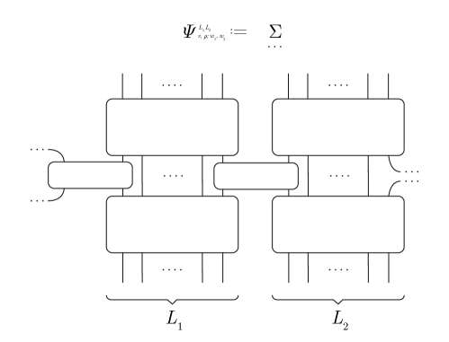
Figure 3: Schematic form of the “defect operators” $\Psi^{L_{1},L_{2}}_{\lambda,\mu;w_{1},w_{2}}$ as MPOs on a bipartite chain of lenghts $L_{1},L_{2}$. The large blocks with $L_{1},L_{2}$ strands are certain representers of the double triangle algebra.

We show that MPOs $\Psi^{L_{1},L_{2}}_{\lambda,\mu;w_{1},w_{2}}$ have several remarkable properties: (i) they commute among each other, i.e. for different $\lambda,\mu$ etc, (ii) they commute with the local densities of the chain Hamiltonian, (iii) they act on a “conformal block” (the range of the projector $Q^{L_{1}}_{\mu_{1},\lambda_{1}}\otimes Q^{L_{2}}_{\mu_{2},\lambda_{2}}$ on the bipartite chain) by fusing in the pair of charges $\lambda,\mu$, (iv) they generate an algebra ${{\cal D}}^{L_{1},L_{2}}$ isomorphic to the “defect algebra” that has been found [4, 5, 60] in the context of $1+1$ dimensional CFTs.

The abelian nature of the defect algebra (i) shows that it is generated by commuting projections $D_{A}^{L_{1},L_{2}}$, and (iv) permits us to import the classification by [4, 5, 60] implying that the minimal projections, $D_{A}^{L_{1},L_{2}}$ are labelled precisely by the simple objects $A$ from ${}_{{\cal M}}X_{{\cal M}}$. By (ii), the subspace onto which a $D_{A}^{L_{1},L_{2}}$ projects is left invariant by the local densities of the Hamiltonian on either side, so it has a sort of “topological character”. By (iii), the generators of the defect algebra ${{\cal D}}^{L_{1},L_{2}}$ of the bipartite chain of lenght $L=L_{1}+L_{2}$ are related to a decomposition

$$\mathscr{V}^{L_{1},L_{2}}=\mathscr{V}^{L_{1}}\otimes\mathscr{V}^{L_{2}},\quad\mathscr{V}^{L_{i}}\cong\bigoplus_{\mu,\lambda:Z_{\lambda,\mu}\neq 0}\mathscr{V}^{L_{i}}_{\lambda,\mu}$$ (11)

of the Hilbert spaces $\mathscr{V}^{L_{i}}$ of each of the two sub-chains $(i=1,2)$, and, on this tensor product Hilbert space the generators $\Psi^{L_{1},L_{2}}_{\lambda,\mu;w_{1},w_{2}}$ of ${{\cal D}}^{L_{1},L_{2}}$ act in a way that is precisely analogous to the “braided product of two full centers” in the CFT context [60]. [Each “full center” [4, 5, 60] in the CFT-context corresponds to decomposing the Hilbert space of the CFT to the left/right of the defect into conformal blocks, and on each side of the defect, the block associated with the primary with highest weight labels $\mu,\lambda$ appears $Z_{\mu,\lambda}$ times (10).] Together, (i)–(iv) suggest to us that the range of $D_{A}^{L_{1},L_{2}}$ in the Hilbert space of the bipartite anyonic chain precisely corresponds to a specific “transparent boundary condition” or “defect”: This defect couples and sits in between the two parts of the bipartite chain, hence at “constant position”.

It is known that the matrix $Z_{\lambda,\mu}$ (10) is equal modular invariant coupling matrix in the CFT context appearing e.g. in the decomposition of the torus partition function $\sum_{\lambda,\mu}Z_{\lambda,\mu}\chi_{\mu}(q)\overline{\chi_{\lambda}(q)}$ or the Hilbert space $\oplus_{\mu,\lambda}Z_{\mu,\lambda}\mathscr{H}^{\rm CFT}_{\mu}\otimes\bar{\mathscr{H}}^{\rm CFT}_{\lambda}$, which in our categorical setting is defined by (10) This suggests that, for a single chain with Hilbert space $\mathscr{V}^{L}$, the subspaces $\mathscr{V}^{L}_{\lambda,\mu}:=Q^{L}_{\lambda,\mu}\mathscr{V}^{L}$ should be generated from $\mathscr{V}^{L}_{0,0}$ by the action of certain local operators on the spin-chain which in the continuum limit ought to have the interpretation of conformal primary operators transforming in the representations $(\lambda,\mu)$ under the Virasoro algebra (assuming ${}_{{{\cal N}}}X_{{{\cal N}}}$ can be identified with a category of Virasoro representations to begin with). Unfortunately, we have as yet not been able to find convincing expressions for such operators.

To summarize the discussion, our results suggest, but of course do not prove, the correspondences

$$\begin{split}&\text{subspaces $Q^{L}_{\mu,\lambda}\mathscr{V}^{L}$}\leftrightarrow\text{CFT conformal block $(\lambda,\mu)$,}\\ &\text{subspaces $D^{L_{1},L_{2}}_{A}\mathscr{V}^{L_{1},L_{2}}$}\leftrightarrow\text{CFT states with defect $A$.}\end{split}$$ (12)

Here, the “CFT” refers to a continuum limit of corresponding anyonic spin chain, should such a limit exist.

If the fusion algebra of ${}_{{\cal N}}X_{{\cal N}}$ is of so-called “Cardy-” or “diagonal type”,

$$Z_{\mu,\lambda}=\delta_{\mu,\lambda},$$ (13)

corresponding in the CFT-context to a simple diagonal sum $\oplus_{\mu}\mathscr{H}^{\rm CFT}_{\mu}\otimes\bar{\mathscr{H}}^{\rm CFT}_{\mu}$, then we show that our defect operators $\Psi^{L_{1},L_{2}}_{\mu,\mu}$ (there are no ‘$w$’-labels in this case) can be labelled equivalently by the objects $A$ of the dual fusion category ${}_{{\cal M}}X_{{\cal M}}$,

$$\mu\leftrightarrow A\quad\text{(diagonal models),}$$ (14)

and our general results imply that they satisfy an algebra precisely isomorphic to (7):

$$\Psi_{A}^{L_{1},L_{2}}\Psi_{B}^{L_{1},L_{2}}=\sum_{C}N_{A,B}^{C}\Psi_{C}^{L_{1},L_{2}}.$$ (15)

Of course, the operators $O^{L}_{A}$ and $\Psi^{L_{1},L_{2}}_{A}$ are not at all the same: The first acts on a single chain of length $L$ whereas the second on a bipartite chain of lengths $L_{1},L_{2}$, so one may tentatively think of the former as associated with “horizontal defects” (inserted at constant time) and of the latter with “vertical defects” (inserted at constant position). For general coupling matrices $Z_{\mu,\lambda}$ our abelian defect algebra ${{\cal D}}^{L_{1},L_{2}}$ appears to us in general different (as an algebra) from the, in general non-abelian, algebra (7) generated by the symmetry operators $O_{A}^{L}$ discussed in connection with defects e.g. in [59, 62, 63], despite the fact that the central projections in our defect algebra ${{\cal D}}^{L_{1},L_{2}}$ are still labelled by the simple objects $A$ of the same category ${}_{{\cal M}}X_{{\cal M}}$. A similar remark applies to the defects constructed in the context of a wide class of lattice models by [64]. It would be interesting to understand the connection to these works better.

At any rate, we find it notable that an exact copy of the defect algebra of $1+1$-dimensional CFTs can be constructed for anyonic spin-chains before the continuum limit, especially in view of the fact that an anyonic spin chain may admit several continuum limits including non-conformal ones. It would be interesting to understand this point better.

1.3 Summary of notations and conventions

The von Neumann algebras appearing in this paper are always assumed to be infinite (type III) factors. ${{\cal N}}\subset{{\cal M}}$ always denotes a finite index inclusion of such von Neumann factors. Calligraphic letters ${{\cal A}},\dots,{{\cal Z}}$ denote algebras, often von Neumann algebras. Operators from a von Neumann algebra will be denoted by lower case Roman letters. The adjoint operation in the von Neumann algebra is denoted by $x\mapsto x^{*}$ whereas the adjoint on the Hilbert space of the spin chain is denoted by $\dagger$. Operators on a spin chain of length $L$ are typically denoted by upper case letters $A^{L},\Phi^{L},\dots$. Upper case Roman indices $A,B,\dots$ also denote endomorphisms from ${{\cal M}}$ and are represented by thick solid lines in wire diagrams, Greek symbols $\mu,\nu,\dots$ denote endomorphisms from ${{\cal N}}$ and are represented by dashed lines. Lower case Roman indices $a,b,\dots$ also denote endomorphisms from ${{\cal N}}\to{{\cal M}}$ and are represented by thin solid lines.

2 Background

2.1 Von Neumann algebras

General definitions: See e.g. [65]. A von Neumann algebra is an ultra-weakly closed $*$-subalgebra of the algebra ${{\cal B}}(\mathscr{H})$ of bounded operators on some Hilbert space, $\mathscr{H}$. The commutant ${{\cal N}}^{\prime}$ of a von Neumann algebra is the von Neumann algebra of all bounded operators on $\mathscr{H}$ commuting with each operator from ${{\cal N}}$. The center of a von Neumann algebra is consequently ${{\cal N}}\cap{{\cal N}}^{\prime}$. A von Neumann algebra with trivial center is said to be a factor. Factors can be classified into types I, II, III; the algebras considered in this work are assumed to be factors of type III. This property is used mainly to set up the calculus of endomorphisms (see below). In QFT, algebras are of this type [50], so the assumption is also natural if we have in mind relating the anyonic spin chain constructions back to QFT.

An inclusion ${{\cal N}}\subset{{\cal M}}$ of von Neumann factors is said to be irreducible if ${{\cal N}}^{\prime}\cap{{\cal M}}$ (also called the first relative commutant) consists of multiples of the identity. We will always assume that we are in this situation when considering inclusions. Associated with any inclusion of factors there is always the “dual inclusion” ${{\cal M}}^{\prime}\subset{{\cal N}}^{\prime}$. For some constructions below, it is also convenient to assume that ${{\cal M}}$ is $\sigma$-finite and in a “standard form”, in the sense that there exists a vector $|\eta\rangle\in\mathscr{H}$ such that both ${{\cal M}}|\eta\rangle$ and ${{\cal M}}^{\prime}|\eta\rangle$ are dense subspaces of $\mathscr{H}$ (in such a case $|\eta\rangle$ is called cyclic and separating). For a von Neumann algebra in standard form one has an anti-linear, unitary, involutive operator $J_{{\cal M}}$ exchanging ${{\cal M}}$ with ${{\cal M}}^{\prime}$ under conjugation (i.e. $j_{{\cal M}}(m)={\rm Ad}(J_{{\cal M}})m:=J_{{\cal M}}mJ_{{\cal M}}\in{{\cal M}}^{\prime}$ iff $m\in{{\cal M}}$). The existence of a cyclic and separating vector is a moderate assumption which we implicitly make throughout.

Conditional expectations: See e.g. [42, 36, 37, 47, 46, 65]. Let ${{\cal N}}\subset{{\cal M}}$ be an irreducible inclusion of two von Neumann factors. An ultraweakly continuous linear operator $E:{{\cal M}}\to{{\cal N}}$ is called a conditional expectation if it is positive, $E(m^{*}m)\geq 0$ for all $m\in{{\cal M}}$, and if

$$E(n_{1}mn_{2})=n_{1}E(m)n_{2}$$ (16)

for $m\in{{\cal M}},n_{i}\in{{\cal N}}$. If there exists any conditional expectation $E$ at all, then the best constant $\lambda>0$ such that

$$E(m^{*}m)\geq\lambda^{-1}m^{*}m\quad\text{for all $m\in{{\cal M}}$}$$ (17)

is called the index of $E$, and there exists one for which $\lambda$ is minimal. This $\lambda=[{{\cal M}}:{{\cal N}}]$ is the Jones-Kosaki index of the inclusion. In this paper we only consider inclusions with a finite index. In such a case one can always define a conditional expectation $E^{\prime}:{{\cal N}}^{\prime}\to{{\cal M}}^{\prime}$ for the dual inclusion.

2.2 Fusion categories, endomorphisms and intertwiner calculus

See e.g. [6, 16, 5, 43, 58, 66]. A fusion category over $\mathbb{C}$ is a monoidal category with finitely many simple objects up to isomorphism and finite-dimensional $\mathbb{C}$-linear morphism spaces, and such that the unit object is simple. Such a category is called unitary if it can be equipped with a $*$-operation such that it becomes a $C^{*}$-category in the sense of [49]. Any such category can be realized as a category of (finite index) endomorphisms of an infinite (type III) von Neumann factor, ${{\cal N}}$, and unitary fusion categories realized in this way will be denoted by ${}_{{\cal N}}X_{{\cal N}}$. An endomorphism $\mu\in{\mathrm{End}}({{\cal N}})$ of a von Neumann algebra ${{\cal N}}$ is an ultra-weakly continuous $*$-homomorphism such that $\mu(1)=1$. It is said to have finite index if $[{{\cal N}}:\mu({{\cal N}})]<\infty$, where the definition of index in the case of type III von Neumann factors is as outlined above. In this paper, all endomorphisms considered are assumed to have a finite index.

Intertwiners ($\to$ Hom-spaces): Given two endomorphisms $\mu,\nu$, one says that a linear operator $t\in{{\cal N}}$ is an “intertwiner” if $t\mu(n)=\nu(n)t$ for all $n\in{{\cal N}}$. The linear space of all such intertwiners is called ${\mathrm{Hom}}_{{\cal N}}(\nu,\mu)$, but note that a given operator $t$ may belong to different Hom-spaces. The subscript ‘${{\cal N}}$’ which indicates the algebra from which the intertwiners are taken is sometimes omitted where clear from the context. For the composition of two endomorphisms we write $\mu\nu:=\mu\circ\nu$. Two endomorphisms are called equivalent if there is a unitary intertwiner between them and irreducible (or simple) if there is no non-trivial self-intertwiner. If $t\in{\mathrm{Hom}}_{{\cal N}}(\mu,\nu)$, then $t^{*}\in{\mathrm{Hom}}_{{\cal N}}(\nu,\mu)$, and if $s\in{\mathrm{Hom}}_{{\cal N}}(\lambda,\sigma)$, then

$$s\times t:=s\sigma(t)=\lambda(t)s\in{\mathrm{Hom}}_{{\cal N}}(\lambda\mu,\sigma\nu)$$ (18)

is called the Doplicher-Haag-Roberts (DHR) product. It is associative, satisfies $(s\times t)^{*}=s^{*}\times t^{*}$, and gives the Hom-spaces the structure of a tensor category. Note that $1_{\sigma}\times t=\sigma(t)$ but $t\times 1_{\sigma}=t$ as operators, where $1_{\sigma}\in{\mathrm{Hom}}(\sigma,\sigma)$ is the trivial intertwiner (equal to the identity operator of ${{\cal N}}$).

Graphical calculus: We often use a graphical calculus for manipulations involving intertwiners. In this calculus, an intertwiner is adjacent to a set of wires which correspond to the input (bottom) and output (top) endomorphisms $\mu,\nu,\dots$. The wires are typically drawn vertically. So for example, in fig. 4, the box represents an intertwiner $t\in{\mathrm{Hom}}(\lambda_{1}\dots\lambda_{m},\mu_{1}\dots\mu_{n})$.

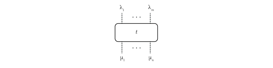
Figure 4: An intertwiner $t\in{\mathrm{Hom}}(\lambda_{1}\dots\lambda_{m},\mu_{1}\dots\mu_{n})$.

The identity intertwiner $1_{\rho}$ is always drawn as a vertical line. To represent the composition of (composable) intertwiners we stack them on top of each other and connect the wires as in fig. 5.

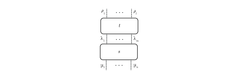
Figure 5: A product $ts$ of intertwiners. The diagram is read from bottom to top.

The DHR product (18) of two intertwiners is written by placing the two wire diagrams horizontally next to each other as in fig. 6.

Figure 6: A DHR product $t\times s$ of intertwiners.

The diagrammatic notation (enriched by various special intertwiners in the following) is designed to automate certain identities. For example:

• We may slide boxes representing intertwiners in a DHR-product vertically upwards or downwards. This corresponds to the equivalent ways of writing the DHR product as in (18).

• If we have an identity between products of intertwiners represented by wired diagrams, we may place an arbitrary number of vertical wires to the left or right (representing a DHR product with $1_{\mu_{1}}\times\cdots 1_{\mu_{n}}\times\cdots$ or $\cdots\times 1_{\mu_{1}}\cdots\times 1_{\mu_{n}}$) to obtain a new identity. This follows from the homomorphism property of the $\mu_{i}$.

• Taking $*$ of an intertwiner represented by a wire diagram means reflection across the horizontal, or reading it top-to-bottom instead of bottom-to-top.

Decomposition: Let $\theta\in{\mathrm{End}}({{\cal N}})$. One writes $\theta\cong\oplus_{\mu}N_{\mu}\,\mu$ if there is a finite set of irreducible and mutually inequivalent endomorphisms $\mu\in{\mathrm{End}}({{\cal N}})$ and isometries $t_{\mu,i}\in{\mathrm{Hom}}_{{\cal N}}(\theta,\mu),i=1,\dots,N_{\mu}:={\mathrm{dim}}_{\mathbb{C}}{\mathrm{Hom}}_{{\cal N}}(\theta,\mu)$ such that $\theta(n)=\sum_{\mu}\sum_{i=1}^{N_{\mu}}t_{\mu,i}\mu(n)t_{\mu,i}^{*}$ for all $n\in{{\cal N}}$, and such that

$$t_{\mu,i}^{*}t_{\nu,j}=\delta_{\mu,\nu}\delta^{i}_{j}1,\quad\sum_{\mu}\sum_{i=1}^{N_{\mu}}t_{\mu,i}t_{\mu,i}^{*}=1,$$ (19)

see fig. 7 for a wire diagram of the second identity and see fig. 8 for a wire diagram of the first identity. Note that for any pair $(\nu,\mu)$ of endomorphisms in ${\mathrm{End}}({{\cal N}})$ with $\nu$ irreducible, the complex linear space ${\mathrm{Hom}}_{{\cal N}}(\mu,\nu)$ is a Hilbert space with inner product

$$t^{*}s=(t,s)1,\quad t,s\in{\mathrm{Hom}}_{{\cal N}}(\mu,\nu),$$ (20)

because $t^{*}s$ is a scalar. Then (19) expresses that $\{t_{\mu,i}:i=1,\dots,N_{\mu}\}$ is an orthonormal basis (ONB) of ${\mathrm{Hom}}_{{\cal N}}(\theta,\mu)$.

Figure 7: Wire diagram for (19).

Figure 8: Wire diagram for (20).

Fusion: Given irreducible $\mu,\nu$ from some unitary fusion category ${}_{{\cal N}}X_{{\cal N}}\subset{\mathrm{End}}({{\cal N}})$, the decomposition into irreducible endomorphisms $\sigma\in_{{\cal N}}X_{{\cal N}}$ is a finite sum as in

$$\mu\nu\cong\bigoplus_{\sigma}N_{\mu,\nu}^{\sigma}\ \sigma,$$ (21)

and the non-negative integers $N_{\mu,\nu}^{\sigma}$ are called the fusion coefficients. They satisfy obvious associativity-type conditions resulting from the associativity of the composition of endomorphisms. Note that it need not be the case that $\mu\nu$ is unitarily equivalent to $\nu\mu$, so the fusion matrices $N_{\mu,\nu}^{\sigma}$ need not be symmetric in the lower indices.

Conjugate and Dimension: Let $\mu\in{\mathrm{End}}({{\cal N}})$ be an irreducible endomorphism of the von Neumann factor ${{\cal N}}$. One calls $\bar{\mu}\in{\mathrm{End}}({{\cal N}})$ a conjugate endomorphism if the fusion of $\mu\bar{\mu}$ and $\bar{\mu}\mu$ contain the identity endomorphism. We assume throughout that the dimension of the endomorphisms considered is finite. This dimension is defined (for example) via the Jones-Kosaki index as $d_{\mu}=[{{\cal N}},\mu({{\cal N}})]^{1/2}$. When the index of $\mu$ is finite, then there exist $r_{\mu},\bar{r}_{\mu}\in{{\cal N}}$ such that $\bar{r}_{\mu}\in{\mathrm{Hom}}_{{\cal N}}(\mu\bar{\mu},id),r_{\mu}\in{\mathrm{Hom}}_{{\cal N}}(\bar{\mu}\mu,id)$ and,

$${\bar{\mu}}(r^{*}_{\mu})\bar{r}_{\mu}=1=\mu(\bar{r}^{*}_{\mu})r_{\mu},\quad r^{*}_{\mu}r_{\mu}=d_{\mu}\cdot 1=\bar{r}^{*}_{\mu}\bar{r}_{\mu}.$$ (22)

In particular, $r_{\mu},\bar{r}_{\mu}$ are multiples of isometries. The second relation gives a relation with the dimension $d_{\mu}\equiv d(\mu)\geq 1$ of $\mu$. One has $d_{\mu}=d_{\bar{\mu}}$ and for $\mu,\nu,\sigma$ irreducible endomorphisms of ${{\cal N}}$,

$$d_{\mu}d_{\nu}=\sum_{\sigma}N_{\mu,\nu}^{\sigma}d_{\sigma}.$$ (23)

These formulas express the additivity/multiplicativity of the quantum dimension under decomposition/fusion and the invariance under conjugation and are the basic justification for the usage of the term “dimension” even though $d_{\mu}$ in general does not have to be integer.

The graphical representation of $r_{\mu},\bar{r}_{\mu}$ is given in fig. 9.

Figure 9: Wire diagrams for $r_{\lambda}^{*},r_{\lambda},\bar{r}_{\lambda}^{*},\bar{r}_{\lambda}$.

The wire diagram for the conjugacy relation is depicted in fig. 10.

Figure 10: Topological invariance of wire diagram representing the conjugacy relation (22).

The wire diagram for the normalization and isometry property of $\bar{r}_{\lambda}$ (similarly for $r_{\lambda}$) is depicted in fig. 11.

Figure 11: Wire diagram for $\bar{r}_{\lambda}^{*}\bar{r}_{\lambda}=d_{\lambda}1$.

Similar constructions can be made if $a$ is an endomorphism from ${{\cal N}}\to{{\cal M}}$, in which case $\overline{a}$ is an endomorphism ${{\cal M}}\to{{\cal N}}$. In either case, one can achieve that $\overline{a\bar{b}}=b\bar{a}$. A generalization to reducible endomorphisms is also possible.

Frobenius duality: Let $\mu,\nu,\lambda\in{\mathrm{End}}({{\cal N}})$ be irreducible and $t\in{\mathrm{Hom}}_{{\cal N}}(\mu\lambda,\nu)$ be normalized to one, $t^{*}t=1$. Then we define a “Frobenius-dual” endomorphism $\tilde{t}\in{\mathrm{Hom}}_{{\cal N}}(\nu\bar{\lambda},\mu)$, see fig. 12,

$$\tilde{t}:=\left(\frac{d_{\nu}}{d_{\mu}}\right)^{-1/2}(t\times 1_{\bar{\lambda}})^{*}(1_{\mu}\times\bar{r}_{\lambda}).$$ (24)

The normalization factor has been chosen so that $\tilde{t}^{*}\tilde{t}=1$. One shows that Frobenius duality is involutive, so we get an anti-isometric identification of intertwiner spaces and corresponding identities between fusion coefficients.

Figure 12: Wire diagram for $\tilde{t}$ given $t$.

Conjugate intertwiner: Let $\mu,\nu,\lambda\in{\mathrm{End}}({{\cal N}})$ be irreducible and $t\in{\mathrm{Hom}}_{{\cal N}}(\mu\lambda,\nu)$ be normalized to one, $t^{*}t=1$. Then we define a “conjugate” endomorphism

$$\bar{t}:=(1_{\bar{\nu}}\times\bar{r}_{\mu})^{*}(1_{\bar{\nu}}\times\bar{r}_{\lambda}\times 1_{\bar{\mu}})^{*}(1_{\bar{\nu}}\times t\times 1_{\bar{\mu}})^{*}(r_{\nu}\times 1_{\bar{\lambda}\bar{\mu}})\in{\mathrm{Hom}}_{{\cal N}}(\bar{\lambda}\bar{\mu},\bar{\nu}).$$ (25)

One shows that the normalization is chosen so that $\bar{t}^{*}\bar{t}=1$, and that conjugation is involutive, so we get an anti-isometric identification of intertwiner spaces and corresponding identities between fusion coefficients.

Braiding: Let ${}_{{\cal N}}X_{{\cal N}}$ be a unitary fusion category. If $\mu\nu\cong\nu\mu$ for any $\mu,\nu\in\,_{{\cal N}}X_{{\cal N}}$ we say the system is braided if a consistent choice of the unitaries implementing the equivalence, called $\varepsilon^{\pm}(\mu,\nu)\in{\mathrm{Hom}}_{{\cal M}}(\mu\nu,\nu\mu)$, i.e. $\mu\nu={\rm Ad}[\varepsilon^{\pm}(\mu,\nu)]\nu\mu$, can be made. Here $\pm$ refer to over- and under-crossing which are the adjoints of each other. If we do not have a superscript as in $\varepsilon(\lambda,\mu)$ then by convention “$+$” is meant. Consistency means that we have the so-called braiding-fusion relations (BFE) and the Yang-Baxter relations (YBE). The YBEs are

$$(1_{\rho}\times\varepsilon(\lambda,\mu))(\varepsilon(\lambda,\rho)\times 1_{\mu})(1_{\lambda}\times\varepsilon(\mu,\rho))=(\varepsilon(\mu,\rho)\times 1_{\nu})(1_{\mu}\times\varepsilon(\lambda,\rho))(\varepsilon(\lambda,\mu)\times 1_{\rho}).$$ (26)

They correspond to the wire diagram in fig. 13.

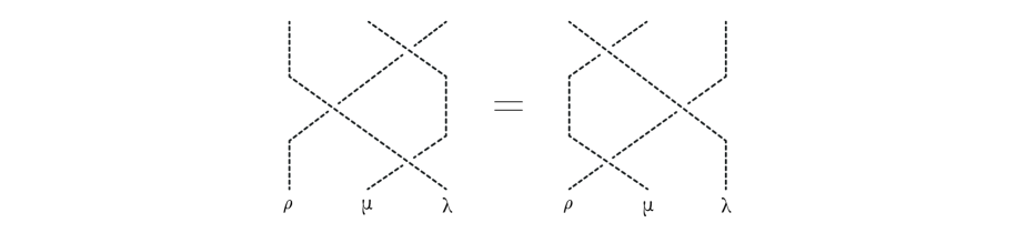
Figure 13: Topological invariance of wire diagram representing the YBE.

The BFEs are ($t\in{\mathrm{Hom}}(\mu\nu,\lambda)$)

$$\begin{split}\varepsilon(\rho,\lambda)(1_{\rho}\times t^{*})&=(t^{*}\times 1_{\rho})(1_{\mu}\times\varepsilon(\rho,\nu))(\varepsilon(\rho,\mu)\times 1_{\nu})\\ \varepsilon(\lambda,\rho)(t^{*}\times 1_{\rho})&=(1_{\rho}\times t^{*})(\varepsilon(\mu,\rho)\times 1_{\nu})(1_{\mu}\times\varepsilon(\nu,\rho))\end{split}$$ (27)

the first of which corresponds to the wire diagram in fig. 14.

Figure 14: Topological invariance of wire diagram representing the BFE. There is a similar diagram with a crossing from right to left and there are similar relations with over-crossings associated with $\varepsilon^{-}(\mu,\nu)$.

We will assume in the following that the braiding is non-degenerate, i.e. $\varepsilon^{\pm}(\lambda,\mu)$ are equal for $\pm$ and all $\mu\in\,_{{\cal N}}X_{{\cal N}}$ if and only if $\lambda=id$. A braiding can be generalized in a natural way to any endomorphism that is decomposable into irreducible endomorphisms from ${}_{{\cal N}}X_{{\cal N}}$. The braiding implies an obvious symmetry of the fusion coefficients.

One has ($\mu\in\,_{{\cal N}}X_{{\cal N}}$):

$$(1_{\mu}\times\bar{r}_{\mu})^{*}(\varepsilon(\mu,\mu)\times 1_{\bar{\mu}})(1_{\mu}\times\bar{r}_{\mu})=e^{2\pi ih(\mu)},$$ (28)

where $h(\mu)\in\mathbb{R}$ is called the statistics phase. For $t\in{\mathrm{Hom}}_{{\cal M}}(\sigma,\mu\nu),\mu,\nu,\sigma\in\,_{{\cal N}}X_{{\cal N}}$, one can show using the BFE and YBE that

$$t\varepsilon(\nu,\mu)\varepsilon(\mu,\nu)=e^{2\pi i(h(\mu)+h(\nu)-h(\sigma))}t.$$ (29)

The Rehren matrix, see fig. 28

$$Y_{\mu,\nu}:=d_{\mu}(1_{\mu}\times\bar{r}_{\nu})^{*}(\varepsilon(\nu,\mu)\varepsilon(\mu,\nu)\times 1_{\bar{\nu}})(1_{\mu}\times\bar{r}_{\nu})$$ (30)

is shown to satisfy $Y_{\mu,\nu}=\sum_{\lambda}d_{\lambda}e^{2\pi i(h(\mu)+h(\nu)-h(\lambda))}N_{\mu,\nu}^{\lambda}$. If the braiding is nondegenerate, ${}_{{\cal N}}X_{{\cal N}}$ is said to be “modular”. In such a case, $Y_{\mu,\nu}$ it is equal up to a prefactor to the Verlinde matrix $S_{\mu,\nu}$ which diagonalizes the fusion coefficients.

2.3 Q-systems and subfactors

Q-systems: See [67, 42, 5]. A Q-system is a way to encode an inclusion of properly infinite von Neumann factors ${{\cal N}}\subset{{\cal M}}$ possessing a minimal conditional expectation $E:{{\cal M}}\to{{\cal N}}$ such that the index, denoted here by $d^{2}$, is finite. An important point is that the data in the Q-system only refer to the smaller factor, ${{\cal N}}$.

Definition 1.

A Q-system is a triple $(\theta,x,w)$ where: $\theta\cong\oplus_{i}\rho_{i}$ is an endomorphism of ${{\cal N}}$, $w\in{\mathrm{Hom}}(\theta,id)\subset{{\cal N}}$ and $x\in{\mathrm{Hom}}(\theta^{2},\theta)\subset{{\cal N}}$ such that

$$w^{*}x=\theta(w^{*})x=1,\quad x^{2}=\theta(x)x,\quad\theta(x^{*})x=xx^{*}=x^{*}\theta(x),$$ (31)

see figs. 15, 16, 17 as well as

$$w^{*}w=d\cdot 1,\quad x^{*}x=d\cdot 1,$$ (32)

see fig. 18.

Figure 15: Wire diagrams for $x^{*}\theta(x)=xx^{*}=\theta(x^{*})x$, which is equivalent to $(x^{*}\times 1_{\theta})(1_{\theta}\times x)=xx^{*}=(1_{\theta}\times x^{*})(x\times 1_{\theta})$ in DHR notation.

Figure 16: Wire diagrams for $x^{2}=\theta(x)x$, which is equivalent to $(x\times 1_{\theta})x=(1_{\theta}\times x)x$ in DHR-notation.

Figure 17: Wire diagrams for $w^{*}x=\theta(w^{*})x=1$, which is equivalent to $(w^{*}\times 1_{\theta})x=(1_{\theta}\times w^{*})x$ in DHR notation.

Figure 18: Wire diagram for $x^{*}x=d1$.

Given a Q-system, one defines an extension ${{\cal M}}$ as follows. As a set, ${{\cal M}}$ consists of all symbols of the form $nv$, where $n\in{{\cal N}}$ with the product, $*$-operation, and unit defined by, respectively

$$n_{1}vn_{2}v=n_{1}\theta(n_{2})xv,\quad(nv)^{*}=w^{*}x^{*}\theta(n^{*})v,\quad 1=w^{*}v.$$ (33)

Associativity and consistency with the $*$-operation follow from the defining relations. The conditional expectation is related to the data by $E(nv)=d^{-1}nw$ and is used to induce the operator norm on ${{\cal M}}$. Conversely, given an inclusion of infinite (type III) factors ${{\cal N}}\subset{{\cal M}}$, the data of the Q-system and $v\in{{\cal M}}$ can be found by a canonical procedure as follows. If $\imath:{{\cal N}}\to{{\cal M}}$ is the inclusion map, we can define a conjugate $\bar{\imath}:{{\cal M}}\to{{\cal N}}$ where $r\in{\mathrm{Hom}}_{{\cal M}}(\bar{\imath}\imath,id)$ and $\bar{r}\in{\mathrm{Hom}}_{{\cal M}}(\imath\bar{\imath},id)$ such that (22) holds with $d=d_{\imath}=[{{\cal M}}:{{\cal N}}]^{1/2}$, namely

$$(\bar{r}^{*}\times 1_{\imath})(1_{\imath}\times r)=1_{\imath},\quad(r^{*}\times 1_{\bar{\imath}})(1_{\bar{\imath}}\times\bar{r})=1_{\bar{\imath}},\quad r^{*}r=d1=\bar{r}^{*}\bar{r}$$ (34)

using the notation of the DHR product (18). Here, and throughout these notes, we use the notation

$$d=[{{\cal M}}:{{\cal N}}]^{1/2}\quad(=d_{\imath}=d_{\theta}^{1/2})$$ (35)

for the square-root of the Jones index. In terms of $r,\bar{r}$, the Q-system for ${{\cal N}}\subset{{\cal M}}$ is now

$$\theta=\bar{\imath}\imath,\quad x=1_{\bar{\imath}}\times\bar{r}\times 1_{\imath}=\bar{\imath}(\bar{r}),\quad w=r.$$ (36)

The relations for this Q-system follow from the relations (34). We work out “explicitly” the very well-known case of an inclusion associated with the action of a finite group $G$ in the appendix as an illustration for the interested reader in app. A.

The defining relations of ${{\cal M}}$ can also be written in a more suggestive way resembling the operator product expansion (OPE) in QFT. Let $\theta\cong\oplus_{i}\rho_{i}$ be the decomposition of $\theta$ into irreducible objects, where a given object may appear multiple times. This means that there are isometries $w_{i}\in{\mathrm{Hom}}(\rho_{i},\theta)$ in ${{\cal N}}$ such that

$$\theta(n)=\sum_{i}w_{i}\rho_{i}(n)w_{i}^{*}.$$ (37)

Next, define $\phi_{i}:=w_{i}^{*}v\in{{\cal M}}$. The defining relations of a Q-system imply

$$\phi_{i}\phi_{j}=\sum_{k}c_{ij}^{k}\,\phi_{k},\quad c_{ij}^{k}:=(w_{i}^{*}\times w^{*}_{j})xw_{k}\in{\mathrm{Hom}}(\rho_{i}\rho_{j},\rho_{k})\cap{{\cal N}}.$$ (38)

Braided product of Q-systems. See [5]. Assume that we have a braiding between the sub-objects $\rho_{i}$ of $\theta$, we can define a braiding operator of $\theta^{2}$ as

$$\varepsilon^{\pm}(\theta,\theta):=\sum_{i,j}(w_{j}\times w_{i})^{*}\varepsilon^{\pm}(\rho_{i},\rho_{j})(w_{i}\times w_{j})\in{\mathrm{Hom}}(\theta^{2},\theta^{2}).$$ (39)

A Q-system for a von Neumann algebra ${{\cal A}}$ is called commutative iff $\varepsilon^{\pm}(\theta,\theta)x=x$. Given two Q-systems $Q_{1}=(\theta_{1},x_{1},w_{1}),Q_{2}=(\theta_{2},x_{2},w_{2})$ and a braiding between the subobjects of $\theta_{1},\theta_{2}$, we can define the braided product Q-system, which has the data

$$(\theta,x^{\pm},w)=Q_{1}\times^{\pm}Q_{2}\quad\Longleftrightarrow$$ (40)

$$\theta=\theta_{1}\theta_{2},\quad x^{\pm}:=(1_{\theta_{1}}\times\varepsilon^{\pm}(\theta_{1},\theta_{2})\times 1_{\theta_{2}})(x_{1}\times x_{2}),\quad w=w_{1}\times w_{2}.$$ (41)

The braided product Q-system is commutative if $Q_{1}$ and $Q_{2}$ both are commutative. The braided product Q-systems define two extension ${{\cal A}}\subset{{\cal B}}_{12}^{\pm}$, which can more explicitly be described as follows: ${{\cal B}}_{12}^{\pm}$ is generated by ${{\cal A}}$ and two isometries $v_{1},v_{2}$ satisfying the relations

$$v_{2}v_{1}=\imath(\varepsilon^{\pm}(\theta_{1},\theta_{2}))v_{1}v_{2},$$ (42)

in addition to the relations for $v_{1},v_{2}$ analogous to (33). It follows that the linear space ${{\cal B}}_{i}^{\pm}:={{\cal A}}v_{i},i=1,2$ define von Neumann algebras intermediate to the braided product extension in the sense that ${{\cal A}}\subset{{\cal B}}_{1}^{\pm},{{\cal B}}_{2}^{\pm}\subset{{\cal B}}_{12}^{\pm}$. The braided product extension plays a role in CFT in the context of defects.

Conditional expectations and canonical endomorphism. See [42]. The minimal conditional expectation $E$ and its dual $E^{\prime}$ can be described more explicitly using Q-systems. In terms of the Q-systems, ${{\cal M}}$ is generated by ${{\cal N}}$ together with a single operator, $v$, and ${{\cal N}}^{\prime}$ is generated by ${{\cal M}}^{\prime}$ together with a single operator, $v^{\prime}$. The operator $v^{\prime}$ can be defined as follows. Let $|\Omega\rangle$ be a cyclic and separating vector for both ${{\cal N}},{{\cal M}}$ (which exists for type III), and let $|\eta\rangle$ be a vector such that $\omega_{\eta}=\omega_{\Omega}\circ E$. Then $v^{\prime}:n|\Omega\rangle\mapsto n|\eta\rangle$ is seen to be an isometry in ${{\cal N}}^{\prime}$, and the dual construction is made for $v\in{{\cal M}}$.

The operators $w=j_{{\cal N}}(v^{\prime})\in{{\cal N}}$, $w^{\prime}=j_{{\cal M}}(v)\in{{\cal M}}^{\prime}$ and the “canonical” endomorphisms

$$\gamma=j_{{\cal N}}j_{{\cal M}}:{{\cal M}}\to{{\cal N}},\quad\gamma^{\prime}=j_{{\cal M}}j_{{\cal N}}:{{\cal N}}^{\prime}\to{{\cal M}}^{\prime}$$ (43)

can be defined, where $j_{{\cal N}}(n)=J_{{\cal N}}nJ_{{\cal N}}$ and $J_{{\cal N}}$ is the modular conjugation of ${{\cal N}}$, etc. The expectations $E,E^{\prime}$ are then given by

$$E(m)=\frac{1}{d}w^{*}\gamma(m)w,\quad E^{\prime}(n^{\prime})=\frac{1}{d}w^{\prime*}\gamma^{\prime}(n^{\prime})w^{\prime}.$$ (44)

They have the property that $J_{{\cal M}}v^{\prime}=v^{\prime}J_{{\cal N}},J_{{\cal M}}v=vJ_{{\cal N}}$. The restricted canonical endomorphism $\theta$ (36) (and similarly for the dual inclusion) is given by

$$\theta=\gamma|_{{{\cal N}}}\in{\rm End}({{\cal N}}),\quad\theta^{\prime}=\gamma^{\prime}|_{{{\cal M}}^{\prime}}\in{\rm End}({{\cal M}}^{\prime}),$$ (45)

for a suitable choice of $\bar{\imath}$ (and $\bar{\imath}^{\prime}$), and for such a choice

$$\theta=\bar{\imath}\imath,\quad\gamma=\imath\bar{\imath}.$$ (46)

$\alpha$-induction: Let ${{\cal N}}\subset{{\cal M}}$ be an irreducible inclusion of subfactors with finite index and associated canonical endomorphism $\theta\in{\mathrm{End}}({{\cal N}})$. Given a braided unitary fusion category ${}_{{\cal N}}X_{{\cal N}}$ and an irreducible endomorphism $\mu\in{}_{{\cal N}}X_{{\cal N}}$ of ${{\cal N}}$, we can define the $\alpha$-induced endomorphisms (of ${{\cal M}}$)

$$\alpha^{\pm}_{\mu}:=\overline{\imath}^{-1}\circ{\rm Ad}(\varepsilon^{\pm}(\mu,\theta))\circ\lambda\circ\overline{\imath},$$ (47)

which is an in general reducible endomorphism of ${{\cal M}}$ (even though $\mu$ is by definition irreducible). If we describe the inclusion $\imath:{{\cal N}}\to{{\cal M}}$ by a Q-system $(\theta=\bar{\imath}\imath,x,w)$, see sec. 2.3, then ${{\cal M}}$ is spanned linearly by elements of the form $nv$ where $n\in{{\cal N}}$ and where $v$ is the generator with the relations recalled in sec. 2.3. Then we can write

$$\alpha^{\pm}_{\lambda}(nv)=\lambda(n)\varepsilon^{\pm}(\lambda,\theta)^{*}v.$$ (48)

One can derive the following naturality/functorial relations:

1. (Conjugate) $\alpha^{\pm}_{\overline{\lambda}}=\overline{\alpha^{\pm}_{\lambda}}$,

2. (Dimension) $d_{\alpha^{\pm}_{\lambda}}=d_{\lambda}$,

3. (Composition) $\alpha^{\pm}_{\lambda}\alpha^{\pm}_{\mu}=\alpha^{\pm}_{\lambda\mu}$,

4. (Functoriality 1) If $t\in{\mathrm{Hom}}(\lambda\mu,\nu)$, then $\imath(t)\in{\mathrm{Hom}}(\alpha^{\pm}_{\lambda\mu},\alpha_{\nu}^{\pm})$,

5. (Braiding) Even though ${{\cal M}}$ is in general not braided, we have ( as endomorphisms of ${{\cal M}}$) $\alpha_{\mu}^{\pm}\alpha^{\pm}_{\lambda}={\rm Ad}(\imath[\varepsilon^{\pm}(\lambda,\mu)])\alpha_{\mu}^{\pm}\alpha^{\pm}_{\lambda}$,

6. (Functoriality 2) if $v\in{\mathrm{Hom}}(\alpha^{-}_{\rho},\alpha^{+}_{\nu}),v^{\prime}\in{\mathrm{Hom}}(\alpha^{-}_{\rho^{\prime}},\alpha^{+}_{\nu^{\prime}})$, then

   $$\imath[\varepsilon^{-}(\rho^{\prime},\rho)](v^{\prime}\times v)=(v\times v^{\prime})\imath[\varepsilon^{+}(\nu,\nu^{\prime})].$$ (49)

The matrix $Z_{\lambda,\mu}:={\mathrm{dim}}{\mathrm{Hom}}(\alpha^{-}_{\lambda},\alpha^{+}_{\mu})$ commutes with the matrix $Y_{\mu,\nu}$ and

$$Z_{\lambda,\mu}\neq 0\quad\Longrightarrow\quad h(\lambda)-h(\mu)\in{\mathbb{Z}}.$$ (50)

2.4 Relative braiding and systems of endomorphisms

See [58, 55, 56, 57, 41]. When studying a finite index inclusion ${{\cal N}}\subset{{\cal M}}$ of von Neumann factors, special systems of endomorphisms often arise. We let $\imath:{{\cal N}}\to{{\cal M}}$ be the embedding and $\overline{\imath}:{{\cal M}}\to{{\cal N}}$ be a conjugate endomorphism. We consider finite sets

$${}_{{\cal N}}X_{{\cal N}} \subset {\mathrm{End}}({{\cal N}},{{\cal N}})\,$$ (51)

$${}_{{\cal M}}X_{{\cal N}} \subset {\mathrm{End}}({{\cal M}},{{\cal N}})\,$$ (52)

$${}_{{\cal N}}X_{{\cal M}} \subset {\mathrm{End}}({{\cal N}},{{\cal M}})\,$$ (53)

$${}_{{\cal M}}X_{{\cal M}} \subset {\mathrm{End}}({{\cal M}},{{\cal M}})\,$$ (54)

of equivalence classes of endomorphisms with the following properties:

• Any two members of any of the sets ${}_{{\cal N}}X_{{\cal M}},{}_{{\cal M}}X_{{\cal N}},{}_{{\cal M}}X_{{\cal M}},{}_{{\cal N}}X_{{\cal N}}$ are mutually inequivalent as endomorphisms, irreducible, and have finite index. [The index of $a\in{\mathrm{End}}({{\cal M}},{{\cal N}})$ is defined as $d_{a}=[{{\cal M}}:a({{\cal N}})]^{1/2}$.]

• ${}_{{\cal N}}X_{{\cal N}}$ is a unitary fusion category and so in particular is closed under fusion and taking conjugates, and so in particular has a unit, the identity endomorphism of ${{\cal N}}$. Additionally, it is assumed to be non-degenerately braided, so the fusion in ${{\cal N}}$ is in particular commutative. Each endomorphism appearing in the decomposition of the canonical endomorphism $\theta=\gamma|_{{\cal N}}=\bar{\imath}\imath$ is required to be contained in ${}_{{\cal N}}X_{{\cal M}}$, and $\varepsilon^{\pm}(\theta,\theta)x=x$, so the Q-system $(\theta,x,w)$ corresponding to ${{\cal N}}\subset{{\cal M}}$ (see sec. 2.3) is commutative in the terminology introduced above. Irreducible objects of ${}_{{\cal N}}X_{{\cal N}}$ will be denoted by lower case Greek letters such as $\mu,\nu,\lambda,\dots$.

• ${}_{{\cal N}}X_{{\cal M}}$ consists of all irreducible endomorphisms $\bar{b}$ (without multiplicities) appearing in the decomposition of $\lambda{\overline{\imath}}$, where $\lambda\in{}_{{\cal N}}X_{{\cal N}}$.

• ${}_{{\cal M}}X_{{\cal N}}$ consists of all irreducible endomorphisms $a$ (without multiplicities) appearing in the decomposition of $\imath\lambda$, where $\lambda\in{}_{{\cal N}}X_{{\cal N}}$.

• ${}_{{\cal M}}X_{{\cal M}}$ consists of all irreducible endomorphisms $B$ (without multiplicities) appearing in the decomposition of $\imath\lambda{\overline{\imath}}$, where $\lambda\in{}_{{\cal N}}X_{{\cal N}}$. Note that by the other assumptions, ${}_{{\cal M}}X_{{\cal M}}$ is by itself a unitary fusion category. But it need not have have a braiding, for example, so the assumptions on ${}_{{\cal M}}X_{{\cal M}}$ respectively ${}_{{\cal N}}X_{{\cal N}}$ are not symmetrical.

Even though the fusion of general endomorphisms of ${{\cal M}}$ may not be commutative (so in particular not braided), we can define a kind of relative braiding between endomorphisms from the sets $\,{}_{{\cal N}}X_{{\cal M}},\,{}_{{\cal M}}X_{{\cal N}},\,{}_{{\cal N}}X_{{\cal N}}$ with the alpha-induced endomorphisms in $\,{}_{{\cal M}}X_{{\cal M}}$. These braiding operators are denoted by

$$\begin{split}\varepsilon^{\pm}(\lambda,\bar{b})&\in{\mathrm{Hom}}(\bar{b}\alpha_{\lambda}^{\pm},\lambda\bar{b})\\ \varepsilon^{\pm}(a,\lambda)&\in{\mathrm{Hom}}(\alpha_{\lambda}^{\pm}a,a\lambda),\end{split}$$ (55)

see [58] sec. 3.3 for the definitions and proofs. Recall that we have defined braiding operators for the alpha induced endomorphisms $\alpha^{\pm}_{\lambda}$ above in (47). Together with (55), these satisfy the expected braiding-fusion (BF) relations, used throughout later parts of this paper, often implicitly when manipulating diagrams. The wire diagrams for the relative braiding intertwiners (55) are depicted in fig. 20. Our conventions for the wires are, see fig. 19,

Figure 19: Types of lines.

• Thick solid lines: Endomorphisms $A,B,\dots$ from ${}_{{\cal M}}X_{{\cal M}}$.

• Thin solid lines: Endomorphisms $a,b,\dots$ or $\bar{a},\bar{b},\dots$ from ${}_{{\cal M}}X_{{\cal N}}$ or ${}_{{\cal N}}X_{{\cal M}}$.

• Dashed lines: Endomorphisms $\mu,\lambda,\dots$ from ${}_{{\cal N}}X_{{\cal N}}$.

Figure 20: Wire diagrams for $\varepsilon^{+}(a,\lambda),\varepsilon^{-}(a,\lambda),\varepsilon^{+}(\lambda,\bar{a}),\varepsilon^{-}(\lambda,\bar{a})$ from left to right.

Using these conventions, the braiding fusion (BF) relatins are depicted in fig. 21.

Figure 21: Topological invariance of wire diagram representing a BF relation with relative braiding. There is a similar BF relation with crossing from right to left.

2.5 Jones basic construction and Jones projections

See e.g. [47, 46, 16, 67, 42] for the extension of Jones’ theory [30] to type III algebras. Consider a finite index inclusion ${{\cal N}}\subset{{\cal M}}$ of type III von Neumann factors in standard form with conditional expectation $E:{{\cal M}}\to{{\cal N}}$. Let $\omega$ be a faithful normal state with cyclic and separating vector $|\Omega\rangle$ for both ${{\cal N}}$ and ${{\cal M}}$ implementing $\omega$. Then $\omega\circ E$ is invariant under $E$, with corresponding vector representative $|\eta\rangle$. Note that $|\eta\rangle$ is not cyclic. $e_{1}:=e_{{{\cal N}}}:=[{{\cal N}}\eta]\in{{\cal N}}^{\prime}$ is called the Jones projection associated with the inclusion and one defines ${{\cal M}}_{1}:={{\cal M}}\vee\{e_{{{\cal N}}}\}$, leading to a new inclusion ${{\cal M}}\subset{{\cal M}}_{1}$. This process is iterated setting $e_{2}:=e_{{{\cal M}}}=[{{\cal M}}\eta]\in{{\cal M}}^{\prime}$ and ${{\cal M}}_{2}:={{\cal M}}_{1}\vee\{e_{{{\cal M}}}\}$, then $e_{3}:=e_{{{\cal M}}_{1}}=[{{\cal M}}_{1}\eta]\in{{\cal M}}_{1}^{\prime}$ and ${{\cal M}}_{3}:={{\cal M}}_{2}\vee\{e_{{{\cal M}}_{1}}\}$ etc. This gives the Jones tower

$${{\cal N}}\subset{{\cal M}}\subset_{e_{1}}{{\cal M}}_{1}\subset_{e_{2}}{{\cal M}}_{2}\subset_{e_{3}}{{\cal M}}_{3}\subset\dots.$$ (56)

One also defines the corresponding Jones tunnel, e.g. by setting

$${{\cal N}}_{1}=j_{{\cal N}}j_{{\cal M}}({{\cal M}}),\quad{{\cal N}}_{2}=j_{{{\cal N}}_{1}}j_{{\cal N}}({{\cal N}}),\quad{{\cal N}}_{3}=j_{{{\cal N}}_{2}}j_{{{\cal N}}_{1}}({{\cal N}}_{1}),\dots$$ (57)

which gives

$$\dots{\cal N}_{3}\subset_{e_{-3}}{{\cal N}}_{2}\subset_{e_{-2}}{{\cal N}}_{1}\subset_{e_{-1}}{{\cal N}}\subset_{e_{0}}{{\cal M}}.$$ (58)

Alternatively, one can construct the Jones tunnel by forming the commutant of the Jones tower for the dual inclusion ${{\cal M}}^{\prime}\subset{{\cal N}}^{\prime}$. $e_{0}=e_{{{\cal N}}_{1}}$ is the projection extending ${{\cal N}}$ to ${{\cal M}}$, $e_{-1}=e_{{{\cal N}}_{2}}$ is that extending ${{\cal N}}_{1}$ to ${{\cal N}}$, $e_{-2}=e_{{{\cal N}}_{3}}$ is that extending ${{\cal N}}_{2}$ to ${{\cal N}}_{1}$ etc. The maps $j_{{\cal N}}j_{{\cal M}}=j_{{{\cal N}}_{1}}j_{{\cal N}}=j_{{{\cal N}}_{2}}j_{{{\cal N}}_{1}}=\dots$ correspond to a 2-shift of the tunnel to the left, so establish that the inclusions ${{\cal N}}\subset{{\cal M}},{{\cal N}}_{2}\subset{{\cal N}}_{1},\dots$ are all isomorphic. The same applies to the inclusions ${{\cal N}}_{1}\subset{{\cal N}}_{2},{{\cal N}}_{3}\subset{{\cal N}}_{4},\dots$. One thereby sees that the endomorphism $\theta=j_{{\cal N}}j_{{\cal M}}$ is a leftwards 2-shift of the even part of the tunnel, giving $\theta^{k}({{\cal N}})={{\cal N}}_{2k}$. Likewise $\gamma=j_{{{\cal M}}}j_{{{\cal M}}_{1}}$ is a leftwards 2-shift of the odd part of the tunnel, giving $\gamma^{k}({{\cal M}})={{\cal N}}_{2k-1}$.

Remembering that the conjugate endomorphism ${\overline{\imath}}$ of the embedding $\imath$ may be chosen such that $\gamma=\imath{\overline{\imath}}$, $\theta=\overline{\imath}\imath$, we therefore get

$$\begin{split}{{\cal N}}_{1}=&\imath{\overline{\imath}}({{\cal M}}),\\ {{\cal N}}_{2}=&\imath{\overline{\imath}}\imath({{\cal N}}),\\ {{\cal N}}_{3}=&\imath{\overline{\imath}}\imath{\overline{\imath}}({{\cal M}}),\\ {{\cal N}}_{4}=&\imath{\overline{\imath}}\imath{\overline{\imath}}\imath({{\cal N}}),\\ &\dots,\end{split}$$ (59)

and so on. The inclusion ${{\cal N}}\subset{{\cal M}}$ is said to be of finite depth if in the subsequent decompositions of $\imath{\overline{\imath}}\imath{\overline{\imath}}\imath{\overline{\imath}}\cdots$ into (equivalence classes of) irreducible endomorphisms $\mu\in{\mathrm{End}}({{\cal M}})$, no new irreducible endomorphisms appear after some “depth” $k$, and this is implied by our standing assumptions formulated in sec. 2.4. (This condition is independent of the condition $d<\infty$ of finite index.)

It is possible to obtain more “concrete” expressions for the Jones projections of the tunnel in terms $r\in{\mathrm{Hom}}_{{\cal M}}(\bar{\imath}\imath,id)$ and $\bar{r}\in{\mathrm{Hom}}_{{\cal M}}(\imath\bar{\imath},id)$ appearing in the the conjugacy relations (34) associated with $\imath,\bar{\imath}$ as follows. First, one can derive the dual identities

$$e_{{{\cal N}}_{1}}=d^{-1}\,vv^{*}=e_{{{\cal M}}^{\prime}},\quad e_{{{\cal M}}_{1}^{\prime}}=d^{-1}\,v^{\prime}v^{\prime*}=e_{{{\cal N}}}.$$ (60)

Now, $e_{{{\cal N}}_{1}}=e_{0}$ whereas $j_{{\cal M}}j_{{{\cal M}}_{1}}(e_{{{\cal M}}_{1}^{\prime}})=j_{{\cal N}}j_{{{\cal M}}}(e_{{{\cal M}}_{1}^{\prime}})=j_{{\cal N}}(e_{{{\cal M}}_{1}^{\prime}})=e_{-1}$. On the other hand, we can show that $v=\bar{r}$ (by using (34)), and we have already mentioned that $j_{{\cal N}}(v^{\prime})=w$, where $v,w$ refer to the Q-system for the extension ${{\cal N}}\subset{{\cal M}}$, and $v^{\prime},w^{\prime}$ to the dual extension ${{\cal M}}^{\prime}\subset{{\cal N}}^{\prime}$. Finally $w=\imath(r)$, and together this gives the first two of the following formulas. The remaining formulas follow by the above observation that $\theta=\bar{\imath}\imath$ ($=$ DHR left mutliplication by $1_{\bar{\imath}}\times 1_{\imath}\times\dots$) respectively $\gamma=\imath\bar{\imath}$ (($=$ DHR left mutliplication by $1_{\imath}\times 1_{\bar{\imath}}\times\dots$)) represent a leftward 2-shift of the Jones tunnel:

$$\begin{split}e_{0}&=d^{-1}\,\bar{r}\bar{r}^{*}\times 1_{\imath}\times 1_{\bar{\imath}}\times\cdots\in{{\cal M}}\cap{{\cal N}}_{1}^{\prime}\\ e_{-1}&=d^{-1}\,1_{\imath}\times rr^{*}\times 1_{\bar{\imath}}\times 1_{\imath}\times\cdots\in{{\cal N}}\cap{{\cal N}}_{2}^{\prime}\\ e_{-2}&=d^{-1}\,1_{\imath}\times 1_{\bar{\imath}}\times\bar{r}\bar{r}^{*}\times 1_{\imath}\times 1_{\bar{\imath}}\times\cdots\in{{\cal N}}_{1}\cap{{\cal N}}_{3}^{\prime}\\ e_{-3}&=d^{-1}\,1_{\imath}\times 1_{\bar{\imath}}\times 1_{\imath}\times rr^{*}\times 1_{\bar{\imath}}\times 1_{\imath}\times\cdots\in{{\cal N}}_{2}\cap{{\cal N}}_{4}^{\prime},\\ &\dots,\end{split}$$ (61)

and so on, where $\times$ is the DHR product, see fig. 22. Note the alternating pattern of $\bar{\imath},\imath$ and $\bar{r},r$. The identity intertwiners $1_{\imath}$ and $1_{\bar{\imath}}$ are inserted to the right in the DHR products to match the vertical lines to the right of the cup-cap pairs in the wire diagram fig. 22, but they do not affect the actual value of $e_{-j}$.

Figure 22: Wire diagram for $e_{-4}$ using the wire diagram for $\bar{r},\bar{r}^{*}$ as in fig. 9 with $\lambda\to\imath$.

Either from (34), or using the diagrams fig. 10 (applied to $\imath,\bar{\imath}$ instead of $\lambda,\bar{\lambda}$) and the value $d=d_{\imath}=d_{\bar{\imath}}$ for the circle, fig. 11, one then gets the Temperly-Lieb-Jones relations (3).

2.6 Higher relative commutants and paths

See e.g. [36, 37] who mainly consider type II case and use bimodule language. The intersections ${{\cal M}}\cap{{\cal N}}_{k}^{\prime}$ and ${{\cal N}}\cap{{\cal N}}^{\prime}_{k+1}$ are called relative commutants. For $k=0$ they are trivial for an irreducible inclusion ${{\cal N}}\subset{{\cal M}}$ of factors, and for $k>0$ they are finite-dimensional matrix algebras if $d<\infty$. The latter can be seen by giving the relative commutants an “explicit” description in terms of intertwining operators.

We first consider the first non-trivial relative commutant ${{\cal N}}\cap{{\cal N}}_{2}^{\prime}$. Consider the decomposition of the endomorphism $\theta=\bar{\imath}\imath\in{\mathrm{End}}({{\cal N}})$ into irreducibles $\mu$ as in (19) using an ONB of intertwiners $t_{\mu,j}\in{\mathrm{Hom}}_{{\cal M}}(\theta,\mu)$. Let $n_{\mu j}^{i}:=t_{\mu,i}(t_{\mu,j})^{*}$. These are matrix units

$$n_{\mu j}^{i}n_{\nu k}^{l}=\delta_{j}^{l}\delta_{\mu,\nu}n_{\mu k}^{i}.$$ (62)

By construction $n_{\nu j}^{i}\in{{\cal N}}\cap{{\cal N}}_{2}^{\prime}$ because they are elements of ${{\cal N}}$ commuting with ${{\cal N}}_{2}=\theta({{\cal N}})$ since they are in ${\mathrm{Hom}}_{{\cal N}}(\theta,\theta)$. In fact these matrix units generate ${{\cal N}}\cap{{\cal N}}_{2}^{\prime}$, so

$${{\cal N}}\cap{{\cal N}}_{2}^{\prime}\cong\bigoplus_{\mu\subset\theta}M_{N_{\mu}}(\mathbb{C}).$$ (63)

We may apply the analogous reasoning to the relative commutant ${{\cal M}}\cap{{\cal N}}_{1}^{\prime}$ using ${{\cal N}}_{1}=\gamma({{\cal M}})$ and a decomposition of $\gamma$ into irreducibles $M$ with intertwiners $t_{M,j}\in{\mathrm{Hom}}(\gamma,M)$. This gives

$${{\cal M}}\cap{{\cal N}}_{1}^{\prime}\cong\bigoplus_{M\subset\gamma}M_{N_{M}}(\mathbb{C}).$$ (64)

Bases for the higher relative commutants ${{\cal M}}\cap{{\cal N}}_{2k+1}^{\prime}$ resp. ${{\cal N}}\cap{{\cal N}}_{2k}^{\prime}$, etc. are obtained by considering the ONBs of intertwiners appearing in subsequent decompositions of $\imath{\overline{\imath}}\imath{\overline{\imath}}\cdots\imath$ resp. ${\overline{\imath}}\imath{\overline{\imath}}\imath\cdots{\overline{\imath}}$, etc. We describe the relative commutants ${{\cal M}}\cap{{\cal N}}_{2k-1}^{\prime}$, the other cases are similar.

By definition, an element of ${{\cal M}}\cap{{\cal N}}_{2k-1}^{\prime}$ is an element of ${{\cal M}}$ that is an intertwiner in the space ${\mathrm{Hom}}((\imath\bar{\imath})^{k},(\imath\bar{\imath})^{k})$. We produce such intertwiners as follows. First, we decompose $\imath\bar{\imath}$ into irreducibles $M_{1}$ an ONB of intertwiners $\{t_{1}\}\subset{\mathrm{Hom}}(\imath{\overline{\imath}},M_{1})$ (more generally we could start with $a_{0}\in\,_{{\cal M}}X_{{\cal N}}$ and decompose $a_{0}\bar{\imath}$). Next we multiply by $\imath$ from the right, and similarly consider an ONB of intertwiners $\{t_{2}\}\subset{\mathrm{Hom}}(M_{1}\imath,a_{2})$, after which we multiply by ${\overline{\imath}}$ from the right, and consider an orthonormal set of intertwiners $\{t_{3}\}\subset{\mathrm{Hom}}(a_{2}{\overline{\imath}},M_{3})$, and so on until $\{t_{2k-1}\}\subset{\mathrm{Hom}}(a_{2k-2}\bar{\imath},M_{2k-1})$. We denote the space of such sequences of isometric intertwiners $(t_{1},t_{2},\dots,t_{2k-1})$ by ${\rm Path}^{2k-1}_{a_{0},M_{2k-1}}$. [The subscript $(a_{0},M_{2k-1})$ means that we start with the object $a_{0}$ and end with $M_{2k-1}$.] Then

$$t_{P}:=(t_{1}\times 1_{\imath}\times 1_{\overline{\imath}}\times\cdots 1_{\overline{\imath}})\cdots(t_{2k-3}\times 1_{\imath}\times 1_{\bar{\imath}})(t_{2k-2}\times 1_{\bar{\imath}})t_{2k-1}\in{\mathrm{Hom}}(a_{0}(\bar{\imath}\imath)^{k-1}\bar{\imath},M_{2k-1}),$$ (65)

where $P$ can be thought of as a “path label” denoting a compatible sequence of orthonormal intertwiners with suitable source and target endomorphisms.

By construction we have (generalizing (19))

$$t_{P}^{*}t_{P^{\prime}}=\delta_{P,P^{\prime}}1,\quad\sum_{P}t_{P}t_{P}^{*}=1.$$ (66)

The desired basis of ${{\cal M}}\cap{{\cal N}}_{2k-11}^{\prime}$ is then $\{t_{P^{\prime}}t_{P}^{*}:P,P^{\prime}\in{\rm Path}^{2k-1}_{\imath,M_{2k-1}}\}$, i.e. the matrix units are labelled by pairs of paths $P,P^{\prime}\in{\rm Path}^{2k-1}_{\imath,M_{2k-1}}$ with the same final object, $M_{2k-1}=M_{2k-1}^{\prime}$.

By fairly obvious variations of the above construction, we could have ended instead with an $a_{2k}\in{}_{{\cal M}}X_{{\cal N}}$ after $2k$ decompositions, or we could have started with $M_{0}\in{}_{{\cal M}}X_{{\cal M}}$, or both. The corresponding path spaces will be denoted accordingly, and this would be related to the other higher relative commutants.

We obviously have a freedom in which order we perform the subsequent decompositions of $\imath{\overline{\imath}}\imath{\overline{\imath}}\cdots\imath$, and a different order of the decomposition gives a different basis, e.g. of ${{\cal M}}\cap{{\cal N}}_{2k-1}^{\prime}$. As in the classical case of group representation, we can pass back and fourth between these bases via $6j$-symbols, which are described below.

2.7 $6j$-symbols

See e.g. [37] (ch. 10, 11) or [40, 39] for the type II case. These references use bimodule language, which can be translated to sectors as outlined in [37], sec. 10.8., but with not many details given. We now consider such $6j$-symbols (also called quantum $6j$-symbols, bi-unitary connections or F-symbols depending on the literature) and discuss some of their properties needed in the sequel. We consider sets of endomorphism ${}_{{\cal N}}X_{{\cal N}},{}_{{\cal N}}X_{{\cal M}},{}_{{\cal M}}X_{{\cal N}},{}_{{\cal M}}X_{{\cal M}}$ as in sec. 2.4. Let $B,M_{1},M_{2}\in\,{}_{{\cal M}}X_{{\cal M}}$, $a_{1},a_{2}\in{}_{{\cal M}}X_{{\cal N}}$. Then we consider the following two ways of decomposing $Ba_{1}{\overline{\imath}}$ as in $(Ba_{1}){\overline{\imath}}$ or $B(a_{1}{\overline{\imath}})$. First, we pick an ONB of intertwiners $t_{1}\in{\mathrm{Hom}}_{{\cal M}}(a_{1}{\overline{\imath}},M_{1})$ and subsequently an ONB of intertwiners $t_{2}\in{\mathrm{Hom}}_{{\cal M}}(BM_{1},M_{2})$. We get an intertwiner

$$(1_{B}\times t_{1})t_{2}\in{\mathrm{Hom}}_{{\cal M}}(Ba_{1}{\overline{\imath}},M_{2}).$$ (67)

Second, we pick an ONB of intertwiners $t_{3}\in{\mathrm{Hom}}_{{\cal M}}(Ba_{1},a_{2})$ and subsequently an ONB of intertwiners $t_{4}\in{\mathrm{Hom}}_{{\cal M}}(a_{2}{\overline{\imath}},M_{2})$. We get an intertwiner

$$(t_{3}\times 1_{\overline{\imath}})t_{4}\in{\mathrm{Hom}}_{{\cal M}}(Ba_{1}{\overline{\imath}},M_{2}).$$ (68)

The intertwiner

$$U_{B}\begin{pmatrix}&t_{1}&\\ t_{3}&&t_{2}\\ &t_{4}&\end{pmatrix}:=[(t_{3}\times 1_{\overline{\imath}})t_{4}]^{*}(1_{B}\times t_{1})t_{2}\in{\mathrm{Hom}}_{{\cal M}}(M_{3},M_{3})=\mathbb{C}1$$ (69)

is a multiple of the identity and identified with a scalar $\mathbb{C}$. It is called a $6j$-symbol, for a wire diagram see fig. 23

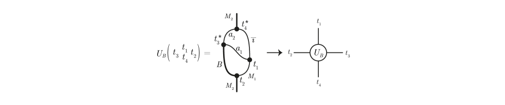
Figure 23: The $6j$-symbol $U_{B}$.

Similarly, let $t_{1}\in{\mathrm{Hom}}(M_{1}\imath,a_{1}),t_{2}\in{\mathrm{Hom}}(BM_{1},M_{2}),t_{3}\in{\mathrm{Hom}}(Ba_{1},a_{2}),t_{4}\in{\mathrm{Hom}}(M_{2}\imath,a_{2})$. Then we set

$$\overline{U}_{B}\begin{pmatrix}&t_{1}&\\ t_{2}&&t_{3}\\ &t_{4}&\end{pmatrix}:=[(t_{2}\times 1_{\imath})t_{4}]^{*}(1_{B}\times t_{1})t_{3}\in{\mathrm{Hom}}_{{\cal M}}(a_{2},a_{2})=\mathbb{C}1.$$ (70)

Lemma 1.

These $6j$-symbols have a number of properties:

1. (Unit): Writing $0=id$ for the identity endomorphism, we have

   $$U_{0}\begin{pmatrix}&t_{1}&\\ t_{3}&&t_{2}\\ &t_{4}&\end{pmatrix}=\delta_{t_{2},1}\delta_{t_{3},1}\delta_{t_{1},t_{4}}.$$ (71)

2. (Unitarity): We have

   $$\sum_{t_{1},t_{2}}U_{B}\begin{pmatrix}&t_{1}&\\ t_{3}&&t_{2}\\ &t_{4}&\end{pmatrix}\overline{U_{B}\begin{pmatrix}&t_{1}&\\ t_{3}^{\prime}&&t_{2}\\ &t_{4}^{\prime}&\end{pmatrix}}=\delta_{t_{4},t_{4}^{\prime}}\delta_{t_{3},t_{3}^{\prime}}$$ (72)

   as well as

   $$\sum_{t_{3},t_{4}}U_{B}\begin{pmatrix}&t_{1}&\\ t_{3}&&t_{2}\\ &t_{4}&\end{pmatrix}\overline{U_{B}\begin{pmatrix}&t_{1}^{\prime}&\\ t_{3}&&t_{2}^{\prime}\\ &t_{4}&\end{pmatrix}}=\delta_{t_{1},t_{1}^{\prime}}\delta_{t_{2},t_{2}^{\prime}}$$ (73)

   where the sums are over an ONB of intertwiners with the appropriate source and target endomorphisms. The contragredient $6j$-symbol is also unitary.

3. (Conjugate): We have

   $$U_{\bar{B}}\begin{pmatrix}&t_{4}&\\ \tilde{t}_{3}&&\tilde{t}_{2}\\ &t_{1}&\end{pmatrix}=\left[\frac{d(a_{1})d(M_{2})}{d(a_{2})d(M_{1})}\right]^{1/2}\overline{U_{B}\begin{pmatrix}&t_{1}&\\ t_{3}&&t_{2}\\ &t_{4}&\end{pmatrix}},$$ (74)

   and similarly

   $$\overline{U}_{\bar{B}}\begin{pmatrix}&t_{4}&\\ \tilde{t}_{3}&&\tilde{t}_{2}\\ &t_{1}&\end{pmatrix}=\left[\frac{d(M_{1})d(a_{2})}{d(M_{2})d(a_{1})}\right]^{1/2}\overline{\overline{U}_{B}\begin{pmatrix}&t_{1}&\\ t_{3}&&t_{2}\\ &t_{4}&\end{pmatrix}}.$$ (75)

Proof.

(Unit) This follows from the ONB properties of the intertwiners and the irreducibility of $M_{i},a_{i},B,{\overline{\imath}},\imath$.

(Unitarity) This follows from the ONB properties of the intertwiners, and their Frobenius duals for the contragredient $6j$-symbols.

(Conjugate) The reader is invited to carry out the following steps in a graphical manner. We begin with the definition of $U_{\bar{B}}$ and the Frobenius dual intertwiners $\tilde{t}_{2},\tilde{t}_{3}$, which allows us to write

$$\begin{split}&U_{\bar{B}}\begin{pmatrix}&t_{4}&\\ \tilde{t}_{3}&&\tilde{t}_{2}\\ &t_{1}&\end{pmatrix}\\ =&\left[\frac{d(a_{1})}{d(a_{2})d(M_{1})d(M_{2})}\right]^{1/2}r^{*}_{M_{1}}(1_{\bar{M}_{1}}\times r_{B}^{*}\times 1_{M_{1}})x(1_{\bar{M}_{1}\bar{B}}\times t_{2}^{*})(1_{\bar{M}_{1}}\times r_{B}\times 1_{M_{1}})r_{M_{1}}.\end{split}$$ (76)

Here we defined $x\in{\mathrm{Hom}}(BM_{1},M_{2})$ as

$$x:=(1_{B}\times t_{1}^{*})(t_{3}\times 1_{\bar{\imath}})t_{4}.$$ (77)

Next we insert a summation over an ONB $s$ of ${\mathrm{Hom}}(BM_{1},M_{3})$ so that the conjugate intertwiner $\bar{s}$ runs over an ONB of ${\mathrm{Hom}}(\bar{M}_{1}\bar{B},\bar{M}_{3})$. This gives us

$$\left[\frac{d(a_{1})}{d(a_{2})d(M_{1})d(M_{2})}\right]^{1/2}\sum_{s,M_{3}}r^{*}_{M_{1}}(1_{\bar{M}_{1}}\times r_{B}^{*}\times 1_{M_{1}})x(\bar{s}\times 1_{M_{2}})(\bar{s}^{*}\times t_{2}^{*})(1_{\bar{M}_{1}}\times r_{B}\times 1_{M_{1}})r_{M_{1}}.$$ (78)

The last three factors in parenthesis yield a $\delta_{s,t_{2}}$ using the definition and isometric property of the conjugate intertwiner, so the summation collapses to $[\dots]^{1/2}r^{*}_{M_{1}}(1_{\bar{M}_{1}}\times r_{B}^{*}\times 1_{M_{1}})(\bar{t}_{2}\times x)r_{M_{2}}$. Next we insert again a summation over an ONB $s$ of ${\mathrm{Hom}}(BM_{1},M_{3})$, turning this into

$$\left[\frac{d(a_{1})}{d(a_{2})d(M_{1})d(M_{2})}\right]^{1/2}\sum_{s,M_{3}}r^{*}_{M_{1}}(1_{\bar{M}_{1}}\times r_{B}^{*}\times 1_{M_{1}})(\bar{t}_{2}\times s)(1_{\bar{M}_{2}}\times s^{*}x)r_{M_{2}}.$$ (79)

We get a $\delta_{s,t_{2}}$ for the same reason as before, so the summation reduces to

$$\left[\frac{d(a_{1})}{d(a_{2})d(M_{1})d(M_{2})}\right]^{1/2}r_{M_{2}}^{*}(1_{\bar{M}_{2}}\times t_{2}^{*}x)r_{M_{2}}=\left[\frac{d(a_{1})d(M_{2})}{d(a_{2})d(M_{1})}\right]^{1/2}\overline{U_{B}\begin{pmatrix}&t_{1}&\\ t_{3}&&t_{2}\\ &t_{4}&\end{pmatrix}}.$$ (80)

The relation for $\overline{U}_{B}$ is demonstrated in the same manner. Note that the intertwiners are not from the same spaces here as in the case of $U_{B}$ and consequently we get a different prefactor. ∎

2.8 Double triangle algebra

See [58], which is partly based on ideas by Ocneanu [34, 33]. Let ${{\cal N}}\subset{{\cal M}}$ be an inclusion of infinite (type III) factors with finite index and finite depth. We consider finite sets ${}_{{\cal N}}X_{{\cal M}},{}_{{\cal M}}X_{{\cal N}},{}_{{\cal M}}X_{{\cal M}},{}_{{\cal N}}X_{{\cal N}}$ of endomorphisms with the properties described in sec. 2.4, where $\imath$ is the embedding endomorphism from ${{\cal N}}\to{{\cal M}}$ and $\bar{\imath}$ a conjugate endomorphism from ${{\cal M}}\to{{\cal N}}$. Note that $a\in{}_{{\cal M}}X_{{\cal N}}$ implies that $\bar{a}\in{}_{{\cal N}}X_{{\cal M}}$.

Definition 2.

As a finite dimensional vector space, the double triangle algebra is defined by

$$\lozenge=\bigoplus_{a,b,c,d\in{}_{{\cal M}}X_{{\cal N}}}{\mathrm{Hom}}_{{\cal M}}(c\bar{d},a\bar{b}).$$ (81)

We note that a given intertwiner might appear in multiple spaces and is considered as different in such a case. It follows from the definition that a basis of $\lozenge$ is given by the elements

$$e_{B;t,b,a}^{s,d,c}:=(d_{a}d_{b}d_{c}d_{d})^{1/4}st^{*},\ \quad s\in{\mathrm{Hom}}_{{\cal M}}(c\bar{d},B),t\in{\mathrm{Hom}}_{{\cal M}}(a\bar{b},B)$$ (82)

where $s,t$ run through an ONB of intertwiners. Our conventions for graphically representing such generators are described in fig. 24.

Figure 24: Left side: wire diagram for a basis element in $\lozenge$, read from bottom to top. Right side: compared to the left diagram, it is rotated by 90 degrees in agreement with the conventions of [58] and stripped off the prefactor. Their conventions are adapted in the following in connection with the double triangle algebras and match the conventions for MPOs and spin chains, which are typically drawn horizontally.

The product structure $\star$ of $\lozenge$ is defined by:

$$e_{B;t,b,a}^{s,b^{\prime},a^{\prime}}\star e_{B^{\prime};t^{\prime},d,c}^{s^{\prime},d^{\prime},c^{\prime}}:=\delta_{b^{\prime},c^{\prime}}\delta_{b,c}(1_{a^{\prime}}\times r_{b^{\prime}}^{*}\times 1_{\bar{d}^{\prime}})(e_{B;t,b,a}^{s,b^{\prime},a^{\prime}}\times e_{B^{\prime};t^{\prime},a,c}^{s^{\prime},a^{\prime},c^{\prime}})(1_{a}\times r_{b}\times 1_{\bar{d}}).$$ (83)

Here $r_{a}\in{\mathrm{Hom}}_{{\cal N}}(\bar{a}a,id)$ are solutions to the conjugacy relations normalized so that $r_{a}^{*}r_{a}=d_{a}1$. The product structure will be depicted graphically by wire diagrams such as fig. 25.

Figure 25: The (vertical) product $\star$ in $\lozenge$.

The unit of $\lozenge$ with respect to the above product structure is given by $\oplus_{a}\bar{r}_{a}\bar{r}_{a}^{*}$, and the structure constants of the double triangle algebra may be obtained by expanding the right side in the the given basis using the intertwiner calculus.

In the literature $\star$ is called the “vertical” product. A “horizontal” product $\cdot$ may be defined by simply using the product structure on (compatible) intertwiners induced by the algebra structure of ${{\cal M}}$, i.e. by $e_{B;t,b,a}^{s,b^{\prime},a^{\prime}}\cdot e_{B^{\prime};t^{\prime},d,c}^{s^{\prime},d^{\prime},c^{\prime}}:=\delta_{a,c^{\prime}}\delta_{b,d^{\prime}}e_{B;t,b,a}^{s,b^{\prime},a^{\prime}}e_{B^{\prime};t^{\prime},a,c}^{s^{\prime},a^{\prime},c^{\prime}}.$ Although this will not be used in this work, we mention that the horizontal and vertical products are related by the “quantum Fourier transform” [36] in a similar way as the pointwise product and convolution of ordinary functions are related by the standard Fourier transfrom.

Definition 3.

${{\cal Z}}_{h}$ is the center of $\lozenge$ with respect to the horizontal product.

[58] have analyzed ${{\cal Z}}_{h}$ in terms of the braiding and fusion relations in ${}_{{\cal N}}X_{{\cal N}}$. As a first result we quote the following. We define

$$e_{B}:=\sum_{t,a,b}e^{t,b,a}_{B;t,b,a}=\bigoplus_{a,b\in{}_{{\cal M}}X_{{\cal N}}}\sqrt{d_{a}d_{b}}\sum_{t\in{\mathrm{Hom}}(a\bar{b},A)}tt^{*},$$ (84)

where the second expression emphasizes the sum is understood as an orthogonal sum as in the orthogonal sum of intertwiner spaces defining $\lozenge$. Then ${{\cal Z}}_{h}=\{e_{B}:B\in_{{\cal M}}X_{{\cal M}}\}$ and it is shown ([58], thm. 4.4) that

$$e_{A}\star e_{B}=\sum_{C}\frac{d_{A}d_{B}}{d_{C}}N_{A,B}^{C}e_{C}$$ (85)

where $A,B,C\in_{{\cal M}}X_{{\cal M}}$ and $N_{A,B}^{C}$ the fusion coefficients. Thus, ${{\cal Z}}_{h}$ is a representation of the fusion ring of ${}_{{\cal M}}X_{{\cal M}}$ under the vertical product.

If ${}_{{\cal N}}X_{{\cal N}}$ is braided as we are assuming, then ${{\cal Z}}_{h}\subset\lozenge$ also contains representations of the fusion rules for ${}_{{\cal N}}X_{{\cal N}}$, as discussed in [58]. Recall from sec. 2.2 that $\alpha^{\pm}_{\lambda}(m)=\bar{\imath}^{-1}\circ\varepsilon^{\pm}(\lambda,\theta)\circ\lambda\circ\bar{\imath}(m),\lambda\in{}_{{\cal N}}X_{{\cal N}},m\in{{\cal M}}$ are the alpha-induced endomorphisms of ${{\cal M}}$ and $\varepsilon^{\pm}(\lambda,\theta)$ the braiding operators of ${}_{{\cal N}}X_{{\cal N}}$. We define the shorthand

$$\langle\alpha^{\pm}_{\lambda},B\rangle:={\mathrm{dim}}{\mathrm{Hom}}_{{\cal M}}(\alpha_{\lambda}^{\pm},B),\quad B\in{}_{{\cal M}}X_{{\cal M}},$$ (86)

and then

$$p_{\lambda}^{\pm}:=d_{\lambda}\sum_{B\in_{{\cal M}}X_{{\cal M}}}d_{B}^{-1}\langle\alpha^{\pm}_{\lambda},B\rangle e_{B}\in\lozenge.$$ (87)

Then clearly $p_{\lambda}^{\pm}\in{{\cal Z}}_{h}$ and it is shown ([58] thm. 5.3 and cor. 5.4) that

$$p_{\mu}^{\pm}\star p_{\nu}^{\pm}=\sum_{\lambda}\frac{d_{\mu}d_{\nu}}{d_{\lambda}}N_{\mu,\nu}^{\lambda}p_{\lambda}^{\pm}$$ (88)

where $\mu,\nu,\lambda\in{}_{{\cal N}}X_{{\cal N}}$ and $N_{\mu,\nu}^{\lambda}$ the fusion coefficients for ${}_{{\cal N}}X_{{\cal N}}$, i.e. for endomorphisms of ${{\cal N}}$. Thus, ${{\cal Z}}_{h}$ contains two ($\pm$) copies of the fusion ring of ${}_{{\cal N}}X_{{\cal N}}$.

Now assume that ${}_{{\cal N}}X_{{\cal N}}$ is in addition non-degenerately braided. Following [58], we define an element $q_{\mu,\nu}\in\lozenge,\mu,\nu\in{}_{{\cal N}}X_{{\cal N}}$ by the following expression (see fig. 26)

$$\begin{split}q_{\mu,\lambda}:=&\sqrt{d_{\mu}d_{\lambda}}D_{X}^{-1}\bigoplus_{a,b\in{}_{{\cal N}}X_{{\cal M}}}\sqrt{d_{a}d_{b}}\sum_{v\in{\mathrm{Hom}}(\alpha^{-}_{\mu},\alpha_{\lambda}^{+})}(1_{a}\times r_{\mu}^{*}\times 1_{\bar{b}})(\varepsilon^{-}(a,\bar{\mu})^{*}\times\varepsilon^{-}(\mu,\bar{b})^{*})\\ &\hskip 56.9055pt(\bar{v}\times 1_{a\bar{b}}\times v)(\varepsilon^{+}(a,\bar{\lambda})\times\varepsilon^{+}(\lambda,\bar{b}))(1_{a}\times r_{\lambda}\times 1_{\bar{b}})\\ =&\bigoplus_{a,b\in{}_{{\cal N}}X_{{\cal M}}}\sqrt{d_{a}d_{b}}\sum_{v\in{\mathrm{Hom}}(\alpha^{-}_{\mu},\alpha_{\lambda}^{+})}q_{\mu,\lambda,v,a,b}\end{split}$$ (89)

where $v\in{\mathrm{Hom}}(\alpha^{-}_{\mu},\alpha_{\lambda}^{+})$ run through an ONB in the sense that for two $v,v^{\prime}$ we have $\imath(r_{\mu}^{*})(\bar{v}\times v^{\prime})\imath(r_{\lambda})=\delta_{v,v^{\prime}}$. Here $\bar{v}=(\imath(r_{\lambda}^{*})\times 1_{\bar{\alpha}^{-}_{\mu}})(1_{\bar{\alpha}_{\lambda}^{+}}\times v^{*}\times 1_{\bar{\alpha}^{-}_{\mu}})(1_{\bar{\alpha}_{\lambda}^{+}}\times\imath(\bar{r}_{\mu}))\in{\mathrm{Hom}}(\bar{\alpha}^{-}_{\mu},\bar{\alpha}_{\lambda}^{+})$ is the conjugate intertwiner. Furthermore, e defined the global index as

$$D_{X}:=\sum_{\mu\in_{{{\cal N}}}X_{{\cal N}}}d_{\mu}^{2}=\sum_{B\in_{{{\cal M}}}X_{{\cal N}}}d_{B}^{2}.$$ (90)

Figure 26: Graphical expression of $q_{\lambda,\mu,v,a,b}$ stripped of the numerical prefactors. In the upper panel, we draw the symbol for this double triangle algebra element rotated by 90 degrees following the conventions of [58]. In the lower panel we draw the normal wire diagram for the intertwiners in $q_{\lambda,\mu,v,a,b}$, to be read from bottom to top.

One of the main results of [58] (thm. 6.9) is that the element $q_{\mu,\nu}\in\lozenge,\mu,\nu\in_{{\cal N}}X_{{\cal N}}$ are mutually commuting idempotents which coincide precisely with the minimal central projections of ${{\cal Z}}_{h}$. Furthermore, identifying ${{\cal Z}}_{h}$ with an orthogonal sum of full matrix algebras as in

$${{\cal Z}}_{h}\cong\bigoplus_{\mu,\nu\in_{{\cal N}}X_{{\cal N}}}M_{Z_{\mu,\nu}}(\mathbb{C}),$$ (91)

the size of each block is precisely $Z_{\mu,\nu}=\langle\alpha^{+}_{\mu},\alpha^{-}_{\nu}\rangle$. Thus, we have, in particular,

$$[q_{\mu,\nu},p^{\pm}_{\lambda}]_{\star}=0,\quad q_{\mu,\nu}\star q_{\mu^{\prime},\nu^{\prime}}=\delta_{\mu,\mu^{\prime}}\delta_{\nu,\nu^{\prime}}q_{\mu,\nu}.$$ (92)

Since $q_{\lambda,\mu}\in{{\cal Z}}_{h}$ which is spanned linearly by the $e_{A}$, there must exist complex coefficients $Y_{\lambda,\mu,A}$ such that

$$q_{\lambda,\mu}=\sum_{A}d^{-1}_{A}Y_{\lambda,\mu,A}e_{A}.$$ (93)

By [58], thm. 6.9, the fusion ring ${}_{{{\cal M}}}X_{{{\cal M}}}$ is abelian (i.e. $AB$ is unitarily equivalent to $BA$ for all $A,B\in{}_{{{\cal M}}}X_{{{\cal M}}}$) if and only if $Z_{\lambda,\mu}\in\{0,1\}$, and in such a case, the simple objects $A\in{}_{{{\cal M}}}X_{{{\cal M}}}$ are in one-to-one correspondence with the pairs of simple objects $(\lambda,\mu)$ from the fusion ring ${}_{{{\cal N}}}X_{{{\cal N}}}$.

We record some properties of $Y_{\lambda,\mu,A}$ in the following lemma for later.

Lemma 2.

The coefficients $Y_{\lambda,\mu,A}\in\mathbb{C}$ as in (93) satisfy:

1. We have, see fig. 27,

   $$Y_{\lambda,\mu,A}=D_{X}^{-1}\sum_{v,a,b,t}d_{a}d_{b}\,t^{*}q_{\mu,\lambda,v,a,b}t,$$ (94)

   where $v$ is running through an ONB of ${\mathrm{Hom}}(\alpha^{+}_{\lambda},\alpha^{-}_{\mu})$, and for fixed $a,b\in{}_{{\cal M}}X_{{\cal N}}$, $t$ is running over an ONB of ${\mathrm{Hom}}(a\bar{b},A)$. $q_{\mu,\lambda,v,a,b}$ is as in (89).

2. $\bar{Y}_{\lambda,\mu,A}=Y_{\lambda,\mu,\bar{A}}$.

3. If the fusion ring ${}_{{{\cal M}}}X_{{{\cal M}}}$ is abelian, then the matrix $Y_{\lambda,\mu,A}$ labelled by simple objects $A\in_{{{\cal M}}}X_{{{\cal M}}}$ and pairs of simple objects $(\lambda,\mu)\in{}_{{{\cal N}}}X_{{{\cal N}}}^{2}$ such that $Z_{\lambda,\mu}\neq 0$ is invertible and unitary up to normalization and their inverse diagonalize the fusion rules of ${}_{{{\cal M}}}X_{{{\cal M}}}$.

Remark: $Y_{\lambda,\mu,A}$ should be thought of as a generalization of Rehren’s matrix $Y_{\rho,\nu}$ (30), under the correspondences $\rho\leftrightarrow(\lambda,\mu),\nu\leftrightarrow A$, as one can appreciate by comparing figs. 27 and 28.

Figure 27: Wire diagram for $Y_{\lambda,\mu,A}$, read from from bottom to top.

Figure 28: Wire diagram for Rehren’s matrix $Y_{\lambda,\mu}$, read from from bottom to top. To go to the rightmost diagram intended to indicate the analogy to fig. 27 for $Y_{\lambda,\nu,A}$, we have used the BF relations.

Proof.

1) It follows by combining (93), (89), and (84) after multiplying (93) from the left with any non-trivial isometry $t\in{\mathrm{Hom}}(a\bar{b},A)$ that $d_{A}^{-1}Y_{\lambda,\mu,A}=\sum_{v}t^{*}q_{\mu,\lambda,v,a,b}t$. Now multiply by $d_{a}d_{b}/D_{X}$ and take a sum over an ONB of $t\in{\mathrm{Hom}}(a\bar{b},A)$ and then a sum over $a,b$. Then we get $(\sum_{a,b}N_{a,\bar{b}}^{A}d_{a}d_{b})d_{A}^{-1}D_{X}^{-1}Y_{\lambda,\mu,A}$ on the left and the claimed formula on the right. The result then follows from $\sum_{a,b}N_{a,\bar{b}}^{A}d_{a}d_{b}=\sum_{a,b}N_{b,A}^{a}d_{a}d_{b}=d_{A}\sum_{b}d_{b}^{2}=d_{A}D_{X}$, using the multiplicative property of the dimension and Frobenius reciprocity.

2) Item 1) shows that $\bar{Y}_{\lambda,\mu,A}=$ the sum over $v$ of the following expression (in the following we us the shorthand $D=D_{X}$):

$$\begin{split}&d_{A}t^{*}q_{\mu,\lambda,v,a,b}^{*}t\\ =&\sqrt{d_{\mu}d_{\lambda}}D^{-1}d_{A}\,t^{*}(1_{a}\times r_{\lambda}^{*}\times 1_{\bar{b}})(\varepsilon^{+}(a,\bar{\lambda})^{*}\times\varepsilon^{+}(\lambda,\bar{b})^{*})\\ &(\bar{v}^{*}\times 1_{a\bar{b}}\times v^{*})(\varepsilon^{-}(a,\bar{\mu})\times\varepsilon^{-}(\mu,\bar{b}))(1_{a}\times r_{\mu}\times 1_{\bar{b}})t\\ =&\sqrt{d_{\mu}d_{\lambda}}D^{-1}\,\bar{r}_{a}^{*}(1_{a}\times r_{b}^{*}\times 1_{\bar{a}})[\\ &(1_{a}\times r_{\lambda}^{*}\times 1_{\bar{b}})(\varepsilon^{+}(a,\bar{\lambda})^{*}\times\varepsilon^{+}(\lambda,\bar{b})^{*})(\bar{v}^{*}\times 1_{a\bar{b}}\times v^{*})\\ &(\varepsilon^{-}(a,\bar{\mu})\times\varepsilon^{-}(\mu,\bar{b}))(1_{a}\times r_{\mu}\times 1_{\bar{b}})t\times\bar{t}]\bar{r}_{A}\\ =&\sqrt{d_{\mu}d_{\lambda}}D^{-1}\,\imath(r_{\lambda}^{*})(1_{\bar{\alpha}^{+}_{\lambda}}\times\bar{r}_{a}^{*}\times 1_{\alpha^{+}_{\lambda}})(1_{\bar{\alpha}^{+}_{\lambda}a}\times r_{b}^{*}1_{\bar{a}\alpha^{+}_{\lambda}})\\ &(1_{\bar{\alpha}^{+}_{\lambda}a\bar{b}\alpha^{+}_{\lambda}}\times\varepsilon^{+}(\lambda,\bar{a})^{*}\times\varepsilon^{+}(b,\bar{\lambda})^{*})(\bar{v}^{*}\times 1_{a\bar{b}}\times v^{*}\times 1_{b\bar{a}})\\ &[(\varepsilon^{-}(a,\bar{\mu})\times\varepsilon^{-}(\mu,\bar{b}))(1_{a}\times r_{\mu}\times 1_{\bar{b}})\times 1_{b\bar{a}}](t\times\bar{t})\bar{r}_{A}\\ =&\sqrt{d_{\mu}d_{\lambda}}D^{-1}\,\imath(r_{\mu}^{*})(1_{\bar{\alpha}^{-}_{\mu}}\times\bar{r}_{a}^{*}\times v)(1_{\bar{\alpha}^{+}_{\lambda}a}\times r_{b}^{*}1_{\bar{a}\alpha^{+}_{\lambda}})\\ &(1_{\bar{\alpha}^{+}_{\lambda}a\bar{b}\alpha^{+}_{\lambda}}\times\varepsilon^{+}(\lambda,\bar{a})^{*}\times\varepsilon^{+}(b,\bar{\lambda})^{*})(1_{\bar{\alpha}^{-}_{\mu}a\bar{b}}\times v^{*}\times 1_{b\bar{a}})\\ &[(\varepsilon^{-}(a,\bar{\mu})\times\varepsilon^{-}(\mu,\bar{b}))(1_{a}\times r_{\mu}\times 1_{\bar{b}})\times 1_{b\bar{a}}](t\times\bar{t})\bar{r}_{A}\\ =&\sqrt{d_{\mu}d_{\lambda}}D^{-1}\,\imath(r_{\mu}^{*})(1_{\bar{\alpha}^{-}_{\mu}}\times\bar{r}_{a}^{*}\times 1_{\alpha^{-}_{\mu}})(\varepsilon^{-}(a,\bar{\mu})^{*}\times r_{b}^{*}1_{\bar{a}}\times v)\\ &(1_{a\bar{\mu}}\times\varepsilon^{-}(\bar{\mu},\bar{b})^{*}\times 1_{b\bar{a}\alpha^{+}_{\lambda}})(1_{a\bar{b}\bar{\alpha}^{-}_{\mu}}\times\bar{v}\times 1_{b\bar{a}\alpha^{+}_{\lambda}})\\ &[1_{a\bar{b}}\times(\varepsilon^{+}(b,\bar{\lambda})\times\varepsilon^{+}(\lambda,\bar{a}))(1_{b}\times r_{\lambda}\times 1_{\bar{a}})](t\times\imath(r_{\lambda})\times\bar{t})\bar{r}_{A}\\ =&\sqrt{d_{\mu}d_{\lambda}}D^{-1}\,\bar{r}_{a}^{*}(1_{a}\times r_{b}^{*}\times 1_{\bar{a}})[\\ &t\times(1_{b}\times r_{\mu}^{*}\times 1_{\bar{a}})(\varepsilon^{-}(b,\bar{\mu})^{*}\times\varepsilon^{-}(\mu,\bar{a})^{*})(\bar{v}\times 1_{b\bar{a}}\times v)\\ &(\varepsilon^{+}(b,\bar{\lambda})\times\varepsilon^{+}(\lambda,\bar{a}))(1_{b}\times r_{\lambda}\times 1_{\bar{a}})\bar{t}]\bar{r}_{A}\\ =&\sqrt{d_{\mu}d_{\lambda}}D^{-1}d_{\bar{A}}\,\bar{t}^{*}(1_{b}\times r_{\mu}^{*}\times 1_{\bar{a}})(\varepsilon^{-}(b,\bar{\mu})^{*}\times\varepsilon^{-}(\mu,\bar{a})^{*})\\ &(\bar{v}\times 1_{b\bar{a}}\times v)(\varepsilon^{+}(b,\bar{\lambda})\times\varepsilon^{+}(\lambda,\bar{a}))(1_{b}\times r_{\lambda}\times 1_{\bar{a}})\bar{t}\\ =&d_{A}\bar{t}^{*}q_{\mu,\lambda,v,b,a}\bar{t}.\end{split}$$ (95)

Here we have used repeatedly the BF relations for the relative braiding operators as described in [58], and the definition of the conjugate intertwiner and the conjugacy relations. The proof becomes more transparent using graphical notation starting from fig. 27, and we will in the following frequently use such a graphical calculus, see e.g. [58]. Now we take the sum over an ONB of $v$’s and then the right side gives exactly $Y_{\lambda,\mu,\bar{A}}$ by item 1) and we are done.

3) This is obvious by [58], thm. 6.9. ∎

2.9 Subfactors and CFTs on $1+1$ Minkowski spacetime

See [50, 42, 16, 15, 10, 9, 68]. In the Haag-Kastler approach to QFT, one can define a $1+1$ CFT by starting from a pair of left-and right-moving copies of a chiral CFT, each given by the Virasoro net $\{{\mathcal{V}}_{c}(I)\}$ where $I$ runs through the open intervals of $S^{1}$. $\{{\mathcal{V}}_{c}(I)\}$ in turn is generated by “quantized diffeomorphisms” of $S^{1}$ which act non-trivially only within the given interval $I$.

More precisely [69], each $\{{\mathcal{V}}_{c}(I)\}$ is a von Neumann algebra acting on a common Hilbert space, $\mathscr{H}$, which is generated by unitary operators $U(f),f\in{\rm Diff}(S^{1})$ subject to the relations $U(f)U(f^{\prime})=e^{icB(f,f^{\prime})}U(f\circ f^{\prime})$, $U(id)=1$, where $f,f^{\prime}$ act non-trivially only within $I$ and where $B:{\rm Diff}(S^{1})\times{\rm Diff}(S^{1})\to\mathbb{R}$ is the Bott cocycle. It is customary to identify the circle $S^{1}\setminus\{-1\}$ minus a point with $\mathbb{R}$ via the Caley transform, and then we can consider the algebras ${{\cal V}}_{c}(I)$ as labelled by open intervals $I\subset\mathbb{R}$. The product of the left and right moving chiral CFTs is labelled by diamonds $D:=\{(t,x)\in\mathbb{R}^{2}\mid t-x\in I_{-},t+x\in I_{+}\}\cong I_{+}\times I_{-}$ where $I_{\pm}$ are open intervals of $\mathbb{R}$, and the algebra of observables of the combined left- and right chiral observables is (see fig. 29)

$${{\cal A}}(D):={{\cal V}}_{c}(I_{+})\otimes{{\cal V}}_{c}(I_{-})^{\rm opp},\quad D\cong I_{+}\times I_{-},$$ (96)

with the appropriate notion of tensor product for von Neumann algebras. Here “opp” means the opposite algebra, which is identical as a vector space but has the opposite product structure $n_{1}\cdot^{\rm opp}n_{2}:=n_{2}n_{1}$ and same $*$-structure.

Figure 29: The causal diamond $D=I_{+}\times I_{-}$.

These algebras are mutually local, i.e. $[{{\cal A}}(D_{1}),{{\cal A}}(D_{2})]=\{0\}$ when $D_{1}$ and $D_{2}$ are space- or timelike related diamonds.

For each open interval $I\subset\mathbb{R}$, we have a system $\Delta_{\rm DHR}(I)$ of irreducible, endomorphisms $\mu$ of ${\mathcal{V}}_{c}(I)$ which are in 1-1 correspondence with irreducible, unitary, highest weight representations of the Virasoro algebra for the central charge $c$. The endomorphisms in $\Delta_{\rm DHR}(I)$ are localized within $I$, i.e. they can be extended to the quasi-local $C^{*}$-algebra generated by all open intervals $J\subset\mathbb{R}$ so as to act as the identity on each ${{\cal V}}_{c}(J)$ for any $J\cap I=\emptyset$. It is known that $\Delta_{\rm DHR}(I)$ forms a modular tensor category.

In the Haag-Kastler approach, a rational CFT in 1+1 Minkowski spacetime is a finite index extension of the net $\{{{\cal A}}(D)\}$, i.e. collection of von Neumann factors

$${{\cal C}}(D)\supset{{\cal A}}(D),$$ (97)

which are again supposed to be mutually local, meaning that $[{{\cal C}}(D_{1}),{{\cal C}}(D_{2})]=0$ for spacelike $D_{1},D_{2}$. It is understood how to construct such an extension from the modular tensor category of transportable endomorphisms $\mu$ of ${\mathcal{V}}_{c}(I)$. First, one shows that due to the transportability and conformal invariance, this extension problem is solved once it is solved for a single, arbitrary reference diamond $D_{0}=I\times I$, that is we only need ${{\cal C}}(D_{0})\supset{{\cal A}}(D_{0})$. The intuitive reason for this is that this diamond can be appropriately moved to any other diamond by means of elements from the group ${\rm Mob}\times{\rm Mob}$, where ${\rm Mob}=\widetilde{{\rm PSL_{2}}(\mathbb{R})}/\{\pm 1\}$, for which one automatically has a strongly continuous unitary representation on $\mathscr{H}\otimes\mathscr{H}$ which acts geometrically on the original net $\{{{\cal A}}(D)\}$ and therefore also on $\{{{\cal C}}(D)\}$.

Accordingly, we set ${{\cal N}}:={{\cal V}}_{c}(I)$, and consider ${{\cal N}}\otimes{{\cal N}}^{\rm opp}(={{\cal A}}(D_{0}))$ where ${{\cal N}}^{\rm opp}$ is the opposite algebra. Then we consider the chosen endomorphisms $\mu$ of ${{\cal N}}$ as defining the modular tensor category ${}_{{\cal N}}X_{{\cal N}}:=\Delta_{\rm DHR}(I)$. Accordingly, we assume that this contains a canonical endomorphism (i.e. a $Q$-system $(\theta,x,w)$) and call $\imath:{{\cal N}}\to{{\cal M}}$ the corresponding extension of ${{\cal N}}$ with embedding $\imath$. The desired extension

$${{\cal C}}\supset{{\cal N}}\otimes{{\cal N}}^{\rm opp}$$ (98)

is defined by the following $Q$-system $Z[X]:=(\theta_{\rm R},x_{\rm R},w_{\rm R})$ [68]. First, the endomorphism $\theta_{\rm R}$ of ${{\cal N}}\otimes{{\cal N}}^{\rm opp}$ is given by

$$\theta_{\rm R}:=\bigoplus_{\lambda,\mu\,_{{\cal N}}X_{{\cal N}}}Z_{\lambda,\mu}\,\lambda\otimes\mu^{\rm opp}\ \ .$$ (99)

The direct sum is understood as follows. For each triple $l=(\lambda,\mu,v)$ with $v$ running through an ONB of ${\mathrm{Hom}}(\alpha^{-}_{\mu},\alpha^{+}_{\lambda})$, we pick an isometry $T_{l}\in{{\cal N}}\otimes{{\cal N}}^{\rm opp}$ such that the relations of a Cuntz algebra are fulfilled,

$$T_{l}^{*}T_{l^{\prime}}=\delta_{l,l^{\prime}}1,\quad\sum_{l}T_{l}T_{l}^{*}=1.$$ (100)

Then we set $\theta_{\rm R}(n\otimes n^{\rm opp})=\sum_{l}T_{l}(\lambda(n)\otimes\mu^{\rm opp}(n^{\rm opp}))T_{l}^{*}$. (Note that the numbers $Z_{\mu,\lambda}\in{\mathbb{N}}_{0}$ are equal to the number of basis elements $v\in{\mathrm{Hom}}(\alpha^{+}_{\mu},\alpha^{-}_{\lambda})$.) The operator $x_{\rm R}\in{\mathrm{Hom}}(\theta_{\rm R},\theta_{\rm R}^{2})$ is

$$x_{\rm R}:=\sum_{l,l^{\prime},l^{\prime\prime}}\sum_{e,f}\eta_{e,f;v,v^{\prime\prime}}^{v^{\prime}}(T_{l}\times T_{l^{\prime}})[\imath(e)\otimes\imath^{\rm opp}(f^{*})]T_{l^{\prime\prime}}^{*}$$ (101)

where $e$ respectively $f$ run through ONBs of ${\mathrm{Hom}}(\lambda\lambda^{\prime},\lambda^{\prime\prime})$ respectively ${\mathrm{Hom}}(\mu\mu^{\prime},\mu^{\prime\prime})$, so that the embeddings $\imath:{{\cal N}}\to{{\cal M}},\imath^{\rm opp}:{{\cal N}}^{\rm opp}\to{{\cal M}}^{\rm opp}$ produce intertwiners in ${\mathrm{Hom}}(\alpha^{-}_{\lambda}\alpha_{\lambda^{\prime}}^{-},\alpha^{-}_{\lambda^{\prime\prime}})$ respectively ${\mathrm{Hom}}(\alpha^{+}_{\mu}\alpha^{+}_{\mu^{\prime}},\alpha^{+}_{\mu^{\prime\prime}})$. $v^{\prime}$ runs through an ONB of ${\mathrm{Hom}}(\alpha^{-}_{\lambda^{\prime}},\alpha^{+}_{\mu^{\prime}})$ (similarly for $v^{\prime\prime}$), $l^{\prime}=(\lambda^{\prime},\mu^{\prime},v^{\prime})$ (similarly for $l^{\prime\prime}$) and Rehren’s structure constants are defined as

$$\eta_{e,f;v,v^{\prime\prime}}^{v^{\prime}}:=\left[\frac{d(\mu)d(\mu^{\prime})}{d(\theta)d(\mu^{\prime\prime})}\right]^{1/2}E[\imath(e)^{*}(v\times v^{\prime})\imath(f)(v^{\prime\prime})^{*}],$$ (102)

with $E:{{\cal M}}\to{{\cal N}}$ the minimal conditional expectation. The properties of $E$ and $\alpha$-induction imply that $\eta_{e,f;v,v^{\prime\prime}}^{v^{\prime}}$ is an intertwiner in ${\mathrm{Hom}}_{{\cal N}}(\lambda,\lambda)$, hence a scalar. The isometry $w_{\rm R}$ is defined to be $T_{id}$. The formula

$$\varepsilon_{\rm R}(\theta_{\rm R},\theta_{\rm R}):=\sum_{l,l^{\prime}}(T_{l}\times T_{l^{\prime}})[\imath(\varepsilon^{+}(\mu,\mu^{\prime}))\times\imath^{\rm opp}(\varepsilon^{-}(\lambda,\lambda^{\prime})^{*})](T_{l^{\prime}}\times T_{l})^{*}$$ (103)

defines a braiding such that $\varepsilon_{\rm R}(\theta_{\rm R},\theta_{\rm R})x_{\rm R}=x_{\rm R}$, i.e. the Q-system $Z[X]:=(\theta_{\rm R},x_{\rm R},w_{\rm R})$ is commutative, and it is in a sense also the maximal such Q-system. It is called the “full center” for this reason and there exists a more abstract, equivalent categorical definition [70]. The summands in the canonical endomorphism $\theta_{\rm R}$ correspond to the “primary fields” by which ${{\cal N}}\otimes{{\cal N}}^{\rm opp}$ has been extended, see sec. 2.3.

We now set ${{\cal C}}(D_{0}):={{\cal C}}$, and by applying appropriate representers of the conformal group, these can be transported from the given diamond $D\subset\mathbb{R}^{2}$ to any other diamond of any shape. Locality of the net $\{{{\cal C}}(D)\}$ is then shown to follow from the commutativity of the Q-system $Z[X]$. Since the numbers $Z_{\mu,\lambda}\in{\mathbb{N}}_{0}$ are equal to the number of basis elements $v\in{\mathrm{Hom}}(\alpha^{+}_{\mu},\alpha^{-}_{\lambda}),$ the independent primary fields are labelled by $(\mu,\lambda,v)$.

2.10 Defects for CFTs on $1+1$ Minkowski spacetime

See [60, 5, 4]. A variant of the above full center Q-system construction can also be employed to construct a $1+1$ CFT in the presence of a transparent defect. In the language of conformal nets this situation is encoded in the following way. We have two finite index nets $\{{{\cal D}}_{l}(D)\}$ and $\{{{\cal D}}_{r}(D)\}$ labeled by causal diamonds $D$ extending the Virasoro-net $\{{{\cal A}}(D)\}$, as above in (97), (96). However, different from above we require Einstein causality only in the restricted sense

$$[{{\cal D}}_{l}(D_{1}),{{\cal D}}_{r}(D_{2})]=\{0\}\quad\text{if $D_{1}$ is left-local to $D_{2}$.}$$ (104)

Here, “left-local” means that $D_{1}$ is not only in the causal complement of $D_{2}$ but also to the left, see fig. 30.

Figure 30: $D_{1}$ is left-local to $D_{2}$. Operators in ${{\cal D}}_{l}(D_{1})$ can be thought of as having a “left shadow”, and operators in ${{\cal D}}_{r}(D_{2})$ a “right shadow”. These shadows must not overlap for commutativity.

The restricted locality encodes that there is somehow a division of the system into a left and a right part and this division is caused by a defect. The defect is topological (so does not have a precise location) and furthermore invisible from the viewpoint of the underlying Virasoro net $\{{{\cal A}}(D)\}$ which remains local in the unrestricted sense.

It turns out that the classification of defects, i.e. finite-index extensions of the Virasoro net subject to the above restricted locality property is achieved by the “braided product”. First, we fix a diamond $D_{0}=I\times I$, where $I$ is some open interval, and we set ${{\cal N}}={{\cal V}}_{c}(I)$, with ${{\cal V}}_{c}$ the Virasoro net, so that ${{\cal A}}(D_{0})$ can be identified with ${{\cal N}}\otimes{{\cal N}}^{\rm opp}$, see sec. 2.3. In ${{\cal N}}\otimes{{\cal N}}^{\rm opp}$, we have the full center Q-system, $Z[X]:=(\theta_{\rm R},x_{\rm R},w_{\rm R})$. Then we take the, say $+$, braided product $Z[X]\times^{+}Z[X]$ of two full center Q-systems, see sec. 2.3. The braided product is a new (commutative) Q-system and thus corresponds to an extension ${{\cal D}}_{12}^{+}$ of ${{\cal N}}\otimes{{\cal N}}^{\rm opp}$. Additionally, we have the intermediate extensions ${{\cal D}}_{1}^{+}$ and ${{\cal D}}_{2}^{+}$, see sec. 2.3. By construction, ${{\cal N}}\otimes{{\cal N}}^{\rm opp}$ is (isomorphic to) ${{\cal A}}(D_{0})$ for a fixed diamond $D_{0}$ and we set ${{\cal D}}_{l}(D_{0}):={{\cal D}}_{1}^{+}$ and ${{\cal D}}_{r}(D_{0}):={{\cal D}}_{2}^{+}$, as well as ${{\cal D}}(D_{0}):={{\cal D}}^{+}_{12}$. This produces only a single pair of inclusions of von Neumann algebras, ${{\cal A}}(D_{0})\subset{{\cal D}}_{l,r}(D_{0})\subset{{\cal D}}(D_{0})$, and not a net of inclusions. But this can again be constructed since the endomorphisms of ${}_{{\cal N}}X_{{\cal N}}$ are transportable. An irreducible defect then corresponds to a central projection in the von Neumann algebra ${{\cal D}}_{12}^{+}$; more precisely, that part of the common Hilbert space $\mathscr{H}\otimes\mathscr{H}$ on which all the algebras ${{\cal D}}_{l,r}(D),{{\cal A}}(D)$ are acting which is the range of the central projection, corresponds to quantum states with a specific “irreducible” topological defect.

A full characterization of the center ${{\cal Z}}({{\cal D}}):={{\cal D}}_{12}^{+}\cap({{\cal D}}_{12}^{+})^{\prime}$ has been given in [60, 5]; in particular these authors have given a presentation of this center as an algebra in terms of generators and relations which we use below. These generators, $B_{\lambda,\mu,w_{1},w_{2}}$, are labelled by a pair of simple objects $\lambda,\mu\in\,_{{\cal N}}X_{{\cal N}}$ and a pair $w_{i}\in{\mathrm{Hom}}(\alpha^{-}_{\mu},\alpha^{+}_{\lambda})$. Thus, the dimension of ${{\cal Z}}({{\cal D}})$ is $\sum_{\mu,\lambda\in\,_{{\cal N}}X_{{\cal N}}}Z_{\mu,\lambda}^{2}$ since ${\mathrm{dim}}{\mathrm{Hom}}(\alpha^{-}_{\mu},\alpha^{+}_{\lambda})=Z_{\mu,\lambda}$, and, because this is also equal to the number of simple objects in $\,{}_{{\cal M}}X_{{\cal M}}$ [58], it suggests that the minimal projections in ${{\cal Z}}({{\cal D}})$ (i.e. irreducible defects) are constructible from the simple objects $A\in\,{}_{{\cal M}}X_{{\cal M}}$. That construction has been given in [60, 5] (thm. 5.5 resp. thm. 4.44), building partly on work by [4].

The details of that construction are broadly as follows. Let $A\in\,_{{\cal M}}X_{{\cal M}}$, so $\beta:=\bar{\imath}B\imath\in\,{}_{{\cal N}}X_{{\cal N}}$ can be defined which defines $m\in{\mathrm{Hom}}(\theta\beta\theta,\beta)$ as $m:=1_{\bar{\imath}}\times\bar{r}\times 1_{B}\times\bar{r}\times 1_{\imath}$, where $\bar{r}\in{\mathrm{Hom}}(\imath\bar{\imath},id)$ is a solution to the conjugacy relations and where $\theta=\bar{\imath}\imath$ is the canonical endomorphism associated with ${{\cal N}}\subset{{\cal M}}$. Then one can define

$$p_{B}:=r_{\beta}^{*}\bar{\beta}\left(\varepsilon^{+}(\theta,\beta)\theta\beta(r_{B}^{*})m\right)r_{\beta}$$ (105)

which is a projection in ${\mathrm{Hom}}(\theta,\theta)$ and the $p_{B}$’s realize a copy of the ${}_{{\cal M}}X_{{\cal M}}$-fusion ring. As is shown in more detail in [60, 5] (thm. 5.5 resp. thm. 4.44), one can obtain from the $p_{B}$ the minimal projections in ${{\cal Z}}({{\cal D}})$ by a canonical procedure based on the observation that ${{\cal Z}}({{\cal D}})\cong{\mathrm{Hom}}(\Theta_{\rm R},\Theta_{\rm R})$.

These minimal projections are not actually used in the present paper but we will show that the for an anyonic spin chain based on the non-degenerately braided fusion category ${}_{{\cal N}}X_{{\cal N}}$ associated with an inclusion of von Neumann factors ${{\cal N}}\subset{{\cal M}}$, we can construct matrix product operators on a bi-partite anyonic spin chain obeying the very same algebraic relations as the generators $B_{\lambda,\mu,w_{1},w_{2}}$ of ${{\cal Z}}({{\cal D}})$. The corresponding projections are then also MPOs, and they determine an orthogonal decomposition of the Hilbert space of the bipartite spin chain. Each summand is invariant under the local operators built from the energy densities, and based on these analogies, we consider the summands, labelled by the simple objects $A\in\,_{{\cal M}}X_{{\cal M}}$, as corresponding to a transparent defect at the level of the chain.

3 MPOs

3.1 $6j$-symbols and MPOs

This subsection follows [29] and [39, 40], which is translated to sector language. We consider sets of endomorphism ${}_{{\cal N}}X_{{\cal N}},{}_{{\cal N}}X_{{\cal M}},{}_{{\cal M}}X_{{\cal N}},{}_{{\cal M}}X_{{\cal M}}$ as in sec. 2.4.

Let $A,B,M_{i}\in{}_{{\cal M}}X_{{\cal M}}$, $a,b,a_{i}\in{}_{{\cal M}}X_{{\cal N}}$. Similar to our discussion of relative commutants, we first decompose $M_{0}\imath$ into irreducibles $a_{1}$ using an ONB of intertwiners $\{t_{1}\}\subset{\mathrm{Hom}}_{{\cal M}}(M_{0}\imath,a_{1})$. Next we multiply by ${\overline{\imath}}$ from the right, and similarly consider an ONB of intertwiners $\{t_{2}\}\subset{\mathrm{Hom}}_{{\cal M}}(a_{1}{\overline{\imath}},M_{2})$, after which we multiply by $\imath$ from the right, and consider an ONB of intertwiners $\{t_{3}\}\subset{\mathrm{Hom}}_{{\cal M}}(M_{2}{\overline{\imath}},a_{3})$, and so on until $\{t_{2k}\}\subset{\mathrm{Hom}}_{{\cal M}}(a_{2k-1}{\overline{\imath}},M_{2k})$, see fig. 1. We denote the space of such sequences of isometric intertwiners $(t_{1},t_{2},\dots,t_{2k})$ with the property $M_{0}=A,M_{2k}=B$ by ${\rm Path}^{2k}_{A,B}$. We also set

$${\rm Path}^{2k}_{c}:=\bigcup_{A\in\,_{{\cal M}}X_{{\cal M}}}{\rm Path}^{2k}_{A,A}$$ (106)

(here “$c$” indicates that we have “closed” paths in a sense). In a similar way, we may start by decomposing $a_{0}\bar{\imath}$ into irreducible objects $M_{1}$ with an ONB $t_{1}\subset{\mathrm{Hom}}_{{\cal M}}(a_{0}\bar{\imath},M_{1})$, then we decompose $M_{1}\imath$ into irreducible objects $a_{2}$ with an ONB $t_{1}\subset{\mathrm{Hom}}_{{\cal M}}(M_{1}\imath,a_{2})$, and so on until $\{t_{2k}\}\subset{\mathrm{Hom}}_{{\cal M}}(M_{2k-1}\imath,a_{2k})$. We denote the space of such sequences of isometric intertwiners $(t_{1},t_{2},\dots,t_{2k})$ with the property $a_{0}=a,a_{2k}=b$ by ${\rm Path}^{2k}_{a,b}$, and we again define the set of closed paths as in (106).

Fixing $k$ and $L=2k$, we consider the following matrices labelled by closed paths $P=(t_{1},t_{2},\dots,t_{L}),P^{\prime}=(t_{1}^{\prime},t_{2}^{\prime},\dots,t_{L}^{\prime})\in{\rm Path}^{L}_{c}$ and $A\in{}_{{\cal M}}X_{{\cal M}}$:

$$\begin{split}&\hskip 85.35826pt(O^{L}_{A})^{P}_{P^{\prime}}:=\\ &\sum_{s_{1},\dots,s_{2L}}\overline{U}_{A}\begin{pmatrix}&t_{1}&\\ s_{1}&&s_{2}\\ &t_{1}^{\prime}&\end{pmatrix}U_{A}\begin{pmatrix}&t_{2}&\\ s_{2}&&s_{3}\\ &t_{2}^{\prime}&\end{pmatrix}\cdots\overline{U}_{A}\begin{pmatrix}&t_{L-1}&\\ s_{2L-1}&&s_{2L}\\ &t_{L-1}^{\prime}&\end{pmatrix}U_{A}\begin{pmatrix}&t_{L}&\\ s_{2L}&&s_{1}\\ &t_{L}^{\prime}&\end{pmatrix}.\end{split}$$ (107)

Here, the $s_{i},i=1,\dots,L/2$ run through ONBs of intertwiners with suitable source and target space. These matrices are identified with linear operators on a finite-dimensional vector space $\mathscr{V}^{L}$:

Definition 4.

(see fig. 1) $\mathscr{V}^{L}$ is the vector space whose basis elements $|t_{1},\dots,t_{L}\rangle=:|P\rangle$ are labelled by $P\in{\rm Path}^{L}_{c}$. $\mathscr{V}^{L}_{\rm open}$ is the is the vector space whose basis elements are labelled by paths $P\in{\rm Path}^{L}_{A,B}$ with $A,B\in\,_{{\cal M}}X_{{\cal M}}$ or by paths $P\in{\rm Path}^{L}_{a,b}$ with $a,b\in\,_{{\cal M}}X_{{\cal N}}$, depending on the context.

Thus, we have for example

$$O^{L}_{A}|P\rangle:=\sum_{P^{\prime}}(O^{L}_{A})^{P}_{P^{\prime}}|P^{\prime}\rangle,$$ (108)

where $P,P^{\prime}\in{\rm Path}^{L}_{c}$. We think of the states $|t_{1},\dots,t_{L}\rangle=:|P\rangle\in\mathscr{V}^{L}_{\rm open}$ as describing the configurations of a spin-chain of length $L$, with the intertwiner $t_{x}$ corresponding the “spin” at “site” $x$. States in the subspace $\mathscr{V}^{L}$ have “periodic boundary conditions”, hence describe states on closed chain, see fig. 1. The MPOs $O_{A}$ thus naturally act on $\mathscr{V}^{L}$ as indicated in fig. 31, but can be extended to $\mathscr{V}^{L}_{\rm open}$ simply by defining their matrix elements to be zero for any non-closed path.

Figure 31: Schematic diagram for the MPO $O_{A}$ representing a map from the outside legs to the inside legs. Here $L=8$.

Note that if $P\in{\rm Path}^{L}_{A,B}$ for some $A,B\in\,_{{\cal M}}X_{{\cal M}}$, the formula (65) gives an intertwiner $t_{P}\in{\mathrm{Hom}}_{{\cal M}}(A(\imath{\overline{\imath}})^{k},B)$. Hence, for $P,P^{\prime}\in{\rm Path}^{L}_{A,B}$, the element $t_{P}^{*}t_{P^{\prime}}$ is a scalar which we define as the inner product $t_{P}^{*}t_{P^{\prime}}=\langle P,P^{\prime}\rangle 1$ on $\mathscr{V}^{L}_{\rm open}$ (or on its subspace $\mathscr{V}^{L}$), turning it into a Hilbert space. The adjoint of a linear operator with respect to this inner product is denoted by a $\dagger$. In view of $\langle P|P^{\prime}\rangle=\delta_{P,P^{\prime}}$ using the ONB properties of the intertwiners, we may simply state this as

$$(A^{\dagger})^{P}_{P^{\prime}}=\overline{A^{P^{\prime}}_{P}}.$$ (109)

The main properties of these matrix product operators (MPOs) are:

Theorem 1.

The MPOs satisfy:

1. (Identity) $O^{L}_{0}=I^{L}$, where “$0$” indicates the identity endomorphism and $I^{L}$ is the identity on $\mathscr{V}^{L}$.

2. (Fusion) For $A,B\in{}_{{\cal M}}X_{{\cal M}}$ and any $k\geq 1,L=2k$:

   $$O^{L}_{A}O^{L}_{B}=\sum_{C\in{}_{{\cal M}}X_{{\cal M}}}N_{A,B}^{C}O^{L}_{C}.$$ (110)

3. (Conjugate) For $A\in{}_{{\cal M}}X_{{\cal M}}$ and any $k\geq 1,L=2k$:

   $$(O^{L}_{A})^{\dagger}=O^{L}_{\bar{A}}.$$ (111)

4. (Projector) Let $D_{X}$ be the global dimension of $X$. Then for any $k\geq 1,L=2k$, the matrix

   $$P^{L}:=\sum_{A\in_{{\cal M}}X_{{\cal M}}}\frac{d_{A}}{D_{X}}O^{L}_{A}$$ (112)

   is an orthogonal projector, $P^{L}=(P^{L})^{\dagger},(P^{L})^{2}=P^{L}$.

Proof.

(Fusion) Let $A,B,C,M_{i},M_{i}^{\prime}\in{}_{{\cal M}}X_{{\cal M}},a_{i}\in{}_{{\cal M}}X_{{\cal N}}$ and consider ONBs of isometric intertwiners

$$\begin{split}t_{0}\in&{\mathrm{Hom}}_{{\cal M}}(C,BA)\\ t_{1}\in&{\mathrm{Hom}}_{{\cal M}}(M_{1},a_{1}{\overline{\imath}}),\\ t_{2}\in&{\mathrm{Hom}}_{{\cal M}}(M_{2},AM_{1}),\\ t_{3}\in&{\mathrm{Hom}}_{{\cal M}}(a_{2},Aa_{1}),\\ t_{4}\in&{\mathrm{Hom}}_{{\cal M}}(M_{2},a_{2}{\overline{\imath}}),\\ t_{5}\in&{\mathrm{Hom}}_{{\cal M}}(a_{3},Ba_{2}),\\ t_{6}\in&{\mathrm{Hom}}_{{\cal M}}(M_{2},a_{3}{\overline{\imath}}),\\ t_{7}\in&{\mathrm{Hom}}_{{\cal M}}(M_{3},BM_{2}),\\ t_{8}\in&{\mathrm{Hom}}_{{\cal M}}(M_{3},CM_{1}),\\ t_{1}^{\prime}\in&{\mathrm{Hom}}_{{\cal M}}(M_{3}^{\prime},a_{1}{\overline{\imath}}),\\ t_{3}^{\prime}\in&{\mathrm{Hom}}_{{\cal M}}(M_{1}^{\prime},AM_{3}^{\prime}),\\ t_{4}^{\prime}\in&{\mathrm{Hom}}_{{\cal M}}(M_{2}^{\prime},a_{2}{\overline{\imath}}),\\ t_{5}^{\prime}\in&{\mathrm{Hom}}_{{\cal M}}(M_{2}^{\prime},BM_{1}^{\prime}),\\ t_{6}^{\prime}\in&{\mathrm{Hom}}_{{\cal M}}(M_{2}^{\prime},a_{3}{\overline{\imath}}),\\ t_{7}^{\prime}\in&{\mathrm{Hom}}_{{\cal M}}(a_{3},Ca_{1}),\\ t_{8}^{\prime}\in&{\mathrm{Hom}}_{{\cal M}}(a_{3},Ca_{1}),\\ t_{8}^{\prime\prime}\in&{\mathrm{Hom}}_{{\cal M}}(M_{2}^{\prime},CM_{3}^{\prime}).\end{split}$$ (113)

To prove the fusion relation, we need the following “zipper lemma”, which is one of the main graphical observations of [29] and algebraically a reinterpretation of the pentagon identity for $6j$-symbols which by definition holds in any unitary fusion category. The “zipper tensors” are defined as

$$Y_{A,B}^{C}\begin{pmatrix}&t_{2}&\\ t_{0};&&t_{8}\\ &t_{7}&\end{pmatrix}:=t_{7}^{*}(1_{B}\times t_{2}^{*})(t_{0}\times 1_{M_{1}})t_{8},\quad\overline{Y}_{A,B}^{C}\begin{pmatrix}&t_{3}&\\ t_{0};&&t_{8}^{\prime}\\ &t_{5}&\end{pmatrix}:=t_{5}^{*}(1_{B}\times t_{3}^{*})(t_{0}\times 1_{a_{1}})t_{8}^{\prime}$$ (114)

and are course also $6j$-symbols (note that the arguments of the unbarred and barred zipper tensor are from different intertwiner spaces).

Figure 32: Schematic diagram for the zipper lemma. Circles represent $6j$-symbols $U$ or $\overline{U}$, whereas the triangle represents the tensors $\overline{Y}$ or $Y$.

Lemma 3.

(Zipper lemma, see fig. 32.) With the intertwiners from the spaces above, we have

$$\begin{split}&\sum_{t_{2},t_{4},t_{7}}U_{A}\begin{pmatrix}&t_{1}&\\ t_{3}&&t_{2}\\ &t_{4}&\end{pmatrix}U_{B}\begin{pmatrix}&t_{4}&\\ t_{5}&&t_{7}\\ &t_{6}&\end{pmatrix}Y_{A,B}^{C}\begin{pmatrix}&t_{2}&\\ t_{0};&&t_{8}\\ &t_{7}&\end{pmatrix}\\ &\hskip 28.45274pt=\ \ \sum_{t_{8}^{\prime}}\overline{Y}_{A,B}^{C}\begin{pmatrix}&t_{3}&\\ t_{0};&&t_{8}^{\prime}\\ &t_{5}&\end{pmatrix}U_{C}\begin{pmatrix}&t_{1}&\\ t_{8}^{\prime}&&t_{8}\\ &t_{6}&\end{pmatrix}\end{split}$$ (115)

and

$$\begin{split}&\sum_{t_{4}^{\prime},t_{3},t_{5}}\overline{U}_{A}\begin{pmatrix}&t_{1}^{\prime}&\\ t_{3}^{\prime}&&t_{3}\\ &t_{4}^{\prime}&\end{pmatrix}\overline{U}_{B}\begin{pmatrix}&t_{4}^{\prime}&\\ t_{5}^{\prime}&&t_{5}\\ &t_{6}^{\prime}&\end{pmatrix}\overline{Y}_{A,B}^{C}\begin{pmatrix}&t_{3}&\\ t_{0};&&t_{8}^{\prime}\\ &t_{5}&\end{pmatrix}\\ &\hskip 28.45274pt=\ \ \sum_{t_{8}^{\prime\prime}}Y_{A,B}^{C}\begin{pmatrix}&t_{3}^{\prime}&\\ t_{0};&&t_{8}^{\prime\prime}\\ &t_{5}^{\prime}&\end{pmatrix}\overline{U}_{C}\begin{pmatrix}&t_{1}^{\prime}&\\ t_{8}^{\prime\prime}&&t_{8}^{\prime}\\ &t_{6}^{\prime}&\end{pmatrix}\end{split}$$ (116)

where the sums are over an ONB of the respective space.

Proof.

The zipper lemma is a version of the pentagon relation. However, we go through the details to show how this works explicitly once, because we will repeat similar manipulations without showing the complete calculations in several places later on. We prove the first relation and begin with, noting that the term in $[\dots]$ already is a scalar,

$$\begin{split}\sum_{t_{1},t_{2},t_{4},t_{7}}&t_{6}^{*}(t_{5}^{*}\times 1_{\overline{\imath}})(1_{B}\times t_{4})t_{7}t^{*}_{7}B[t_{4}^{*}(t_{3}^{*}\times 1_{\overline{\imath}})(1_{A}\times t_{1})t_{2}]B(t_{2}^{*}(1_{A}\times t_{1}^{*}))\\ =&\ t_{6}^{*}(t_{5}^{*}\times 1_{\overline{\imath}})(1_{B}\times t_{3}^{*}\times 1_{\overline{\imath}})\end{split}$$ (117)

which follows from the ONB properties of the intertwiners and which can be rewritten as

$$\sum_{t_{1},t_{2},t_{4},t_{7}}U_{A}\begin{pmatrix}&t_{1}&\\ t_{3}&&t_{2}\\ &t_{4}&\end{pmatrix}U_{B}\begin{pmatrix}&t_{4}&\\ t_{5}&&t_{7}\\ &t_{6}&\end{pmatrix}t_{7}^{*}(1_{B}\times t_{2}^{*})(1_{B}\times 1_{A}\times t_{1}^{*})=t_{6}^{*}(t_{5}^{*}\times 1_{\overline{\imath}})(1_{B}\times t_{3}^{*}\times 1_{\overline{\imath}}).$$ (118)

Now we multiply with $t_{0}$ from the right on both sides. On the left, we use:

$$t_{7}^{*}(1_{B}\times t_{2}^{*})(1_{B}\times 1_{A}\times t_{1}^{*})(t_{0}\times 1_{1}\times 1_{\overline{\imath}})=\sum_{t_{8}}Y_{A,B}^{C}\begin{pmatrix}&t_{2}&\\ t_{0};&&t_{8}\\ &t_{7}&\end{pmatrix}t_{8}^{*}(1_{C}\times t_{1}^{*}).$$ (119)

On the right side we use:

$$t_{6}^{*}(t_{5}^{*}\times 1_{\overline{\imath}})(1_{B}\times t_{3}^{*}\times 1_{\overline{\imath}})(t_{0}\times 1_{1}\times 1_{\overline{\imath}})=\sum_{t_{8}^{\prime}}Y_{A,B}^{C}\begin{pmatrix}&t_{5}&\\ t_{0};&&t_{8}^{\prime}\\ &t_{3}&\end{pmatrix}t_{6}^{*}(t_{8}^{\prime}{}^{*}\times 1_{\overline{\imath}}).$$ (120)

On the term on the right we next use:

$$t_{6}^{*}(t_{8}^{\prime}{}^{*}\times 1_{\overline{\imath}})=\sum_{t_{1},t_{8}}U_{C}\begin{pmatrix}&t_{1}&\\ t_{8}^{\prime}&&t_{8}\\ &t_{6}&\end{pmatrix}t_{8}^{*}(1_{C}\times t_{1}^{*}).$$ (121)

Putting these identities together yields the result. The second identity is proven in a similar way. ∎

To finish the proof of (fusion), we consider the following orthogonality relations

$$\sum_{C}\sum_{t_{8},t_{0}}Y_{A,B}^{C}\begin{pmatrix}&t_{2}&\\ t_{0};&&t_{8}\\ &t_{7}&\end{pmatrix}\overline{Y_{A,B}^{C}\begin{pmatrix}&t_{2}^{\prime}&\\ t_{0};&&t_{8}\\ &t_{7}^{\prime}&\end{pmatrix}}=\delta_{t_{2},t_{2}^{\prime}}\delta_{t_{7},t_{7}^{\prime}},$$ (122)

and

$$\sum_{t_{2},t_{7}}Y_{A,B}^{C}\begin{pmatrix}&t_{2}&\\ t_{0};&&t_{8}\\ &t_{7}&\end{pmatrix}\overline{Y_{A,B}^{C}\begin{pmatrix}&t_{2}&\\ t_{0};&&t_{8}^{\prime}\\ &t_{7}&\end{pmatrix}}=\delta_{t_{8},t_{8}^{\prime}},$$ (123)

which follow from the ONB properties of the intertwiners. Similar relations hold for the barred zipper tensor. Then we look at a matrix element of the product $O^{L}_{A}O^{L}_{B}$, and insert the first orthogonality relation for the zipper tensor. The matrix element is labelled by closed paths $P=(t_{1},t_{2},\dots,t_{L}),P^{\prime\prime}=(t_{1}^{\prime\prime},t_{2}^{\prime},\dots,t_{L}^{\prime\prime})\in{\rm Path}^{L}_{c}$

$$\begin{split}(O^{L}_{A}O_{B}^{L})^{P}_{P^{\prime\prime}}=&\ \sum_{s_{i},s_{j}^{\prime},t_{k}^{\prime}}\sum_{C}\ \sum_{u,t_{0}}\ Y_{A,B}^{C}\begin{pmatrix}&s_{1}&\\ t_{0};&&u\\ &s_{1}^{\prime}&\end{pmatrix}\overline{Y_{A,B}^{C}\begin{pmatrix}&s_{L}&\\ t_{0};&&u\\ &s^{\prime}_{L}&\end{pmatrix}}\\ &\cdot\ \prod_{i=0}^{L/2}\overline{U}_{A}\begin{pmatrix}&t_{2i-1}&\\ s_{2i-1}&&s_{2i}\\ &t_{2i-1}^{\prime}&\end{pmatrix}\overline{U}_{B}\begin{pmatrix}&t_{2i-1}^{\prime}&\\ s_{2i-1}^{\prime}&&s_{2i}^{\prime}\\ &t_{2i-1}^{\prime\prime}&\end{pmatrix}\\ &\cdot\ \prod_{j=0}^{k}U_{A}\begin{pmatrix}&t_{2j}\ \ &\\ s_{2j}\ \ &&s_{2j+1}\\ &t_{2j}^{\prime}\ \ &\end{pmatrix}U_{B}\begin{pmatrix}&t_{2j}^{\prime}\ \ &\\ s_{2j}^{\prime}\ \ &&\ s_{2j+1}^{\prime}\\ &t_{2j}^{\prime\prime}\ \ &\end{pmatrix}\end{split}$$ (124)

On this expression, we apply the zipper lemma $L$ times, and then we use the second orthogonality relation of the zipper tensor, giving an expression which no longer depends on $t_{0}$. The sum over $t_{0}\in{\mathrm{Hom}}_{{\cal M}}(AB,C)$ then yields the prefactor $N_{A,B}^{C}={\mathrm{dim}}_{\mathbb{C}}{\mathrm{Hom}}_{{\cal M}}(AB,C)$.

(Conjugate): This follows from the property (conjugate) of thm. 1. Note that we must use the precise form of the quartic root prefactors.

(Projector): $P^{L}=(P^{L})^{\dagger}$ follows from (conjugate). We have

$$(P^{L})^{2}=\sum_{A,B,C\in_{{\cal M}}X_{{\cal M}}}N_{A,B}^{C}\frac{d_{A}d_{B}}{D_{X}^{2}}O_{C}^{L}$$ (125)

using (fusion). Frobenius reciprocity gives $N_{A,B}^{C}=N_{\bar{A},C}^{B}$ and hence $\sum_{B}N_{A,B}^{C}d_{B}=d_{\bar{A}}d_{C}=d_{A}d_{C}$. So $\sum_{A,B}N_{A,B}^{C}d_{B}d_{A}=D_{X}d_{C}$ and $(P^{L})^{2}=P^{L}$ follows. ∎

3.2 MPOs and double triangle algebra

In this subsection, we define an extended class of MPOs which giving a representation of the double triangle algebra and of the fusion rings ${}_{{\cal M}}X_{{\cal M}}$ and ${}_{{\cal N}}X_{{\cal N}}$, and not just of ${}_{{\cal M}}X_{{\cal M}}$ as in the previous subsection. As in that subsection, we consider the finite sets ${}_{{\cal N}}X_{{\cal M}},_{{\cal M}}X_{{\cal N}},_{{\cal M}}X_{{\cal M}},_{{\cal N}}X_{{\cal N}}$ of endomorphisms with the properties listed in sec. 2.4, and paths $P=(t_{1},\dots,t_{L})\in{\rm Path}_{a^{\prime},a}$ and $P^{\prime}=(t_{1}^{\prime},\dots,t_{L}^{\prime})\in{\rm Path}_{b^{\prime},b}.$

Fixing an even number $L$, we consider the linear operators on $\mathscr{V}^{L}_{\rm open}$ defined by the following matrix elements, see fig. 33:

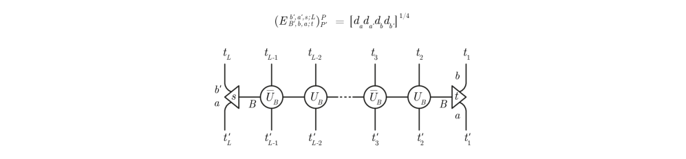
Figure 33: The matrix element $\langle t_{L},\dots,t_{1}|E^{b^{\prime},a^{\prime},s;L}_{B;b,a,t}|t_{L}^{\prime},\dots,t_{1}^{\prime}\rangle$ of the symmetry operator (MPO). Here ‘$P$’ indicates the “path” of intertwiners $t_{L},\dots,t_{1}$.

$$\begin{split}&(E^{b^{\prime},a^{\prime},s;L}_{B;b,a,t})^{P}_{P^{\prime}}:=[d(a)d(b)d(a^{\prime})d(b^{\prime})]^{1/4}\sum_{s_{1},\dots,s_{L+1}}\cdot\\ &\cdot\ Z_{a^{\prime},\bar{b}^{\prime}}^{B}\begin{pmatrix}&t_{1}&\\ s;&&s_{1}\\ &t_{1}^{\prime}&\end{pmatrix}\prod_{j=1}^{k}\left\{\overline{U}_{B}\begin{pmatrix}&t_{2j-1}&\\ s_{2j-1}&&s_{2j}\\ &t_{2j-1}^{\prime}&\end{pmatrix}U_{B}\begin{pmatrix}&t_{2j}&\\ s_{2j}&&s_{2j+1}\\ &t_{2j}^{\prime}&\end{pmatrix}\right\}Z_{a,\bar{b}}^{B}\begin{pmatrix}&&t_{L}\\ t;&s_{L+1}&\\ &&t_{L}^{\prime}\end{pmatrix}.\end{split}$$

Here the labels $E^{b^{\prime},a^{\prime},s;L}_{B;b,a,t}$ correspond to those on $e^{b^{\prime},a^{\prime},s}_{B;b,a,t}$ in the definition of the double triangle algebra, and the matrix elements are set to zero for all other paths whose beginning and endpoints do not match with $a,a^{\prime},b,b^{\prime}$ as above. $Z_{a,\bar{b}}^{B}$ is another type of $6j$-symbol defined as follows (see fig. 34).

Figure 34: The $6j$-symbol $Z_{a,\bar{b}}^{B}$.

$A_{1},A_{2},B\in\ _{{\cal M}}X_{{\cal M}},a,b,c\in\ _{{\cal M}}X_{{\cal N}}$ and $u_{1}\in{\mathrm{Hom}}(a\overline{\imath},A_{1}),u_{2}\in{\mathrm{Hom}}(BA_{2},A_{1}),u_{3}\in{\mathrm{Hom}}(b\overline{\imath},A_{2}),t\in{\mathrm{Hom}}(a\bar{b},B)$. Then we define

$$Z_{a,\bar{b}}^{B}\begin{pmatrix}&&u_{3}\\ t;&u_{2}&\\ &&u_{1}\end{pmatrix}=u_{2}^{*}(t^{*}\times u_{3}^{*})(1_{a}\times r_{b}\times 1_{\bar{\imath}})u_{1}$$ (126)

which is up to a prefactor equal to the complex conjugate of the $6j$-symbol $U_{B}\begin{pmatrix}&u_{3}&\\ t&&u_{2}\\ &u_{1}&\end{pmatrix}$ as can be seen from Frobenius duality. The corresponding $Z$-type $6j$ symbol with the rearranged pattern of the indices is its complex conjugate (with the corresponding substitution of the intertwiners). The sum runs over a complete ONB of intertwiners in Hom-spaces compatible with the source and target spaces of $t_{i},t_{i}^{\prime}$ implicit in the definitions of the path spaces. Our main observation in this section is the following:

Theorem 2.

For any even $L=2k$, the map $\pi^{L}:\lozenge\to{\mathrm{End}}(\mathscr{V}^{L}_{\rm open}),e^{b^{\prime},a^{\prime},s}_{B;b,a,t}\mapsto E^{b^{\prime},a^{\prime},s;L}_{B;b,a,t}$ is a representation of $(\lozenge,\star)$.

Proof.

We let $B,B^{\prime},B^{\prime\prime},M_{1},M_{2},M_{1}^{\prime},M_{2}^{\prime}\in{}_{{\cal M}}X_{{\cal M}}$, $a,b,c,d\in{}_{{\cal M}}X_{{\cal N}}$, and consider the following intertwiners:

$$\begin{split}&t\in{\mathrm{Hom}}_{{\cal M}}(a\bar{b},B),\\ &t^{\prime}\in{\mathrm{Hom}}_{{\cal M}}(c\bar{a},B^{\prime}),\\ &t^{\prime\prime}\in{\mathrm{Hom}}_{{\cal M}}(B^{\prime}B,B^{\prime\prime}),\\ &t^{\prime\prime\prime}\in{\mathrm{Hom}}_{{\cal M}}(c\bar{b},B^{\prime\prime}),\\ &s_{1}\in{\mathrm{Hom}}_{{\cal M}}(a\overline{\imath},M_{1}),\\ &s_{2}\in{\mathrm{Hom}}_{{\cal M}}(b\overline{\imath},M_{2}),\\ &s_{3}\in{\mathrm{Hom}}_{{\cal M}}(BM_{2},M_{1}),\\ &s_{2}^{\prime}\in{\mathrm{Hom}}_{{\cal M}}(c\overline{\imath},M_{1}^{\prime}),\\ &s_{3}^{\prime}\in{\mathrm{Hom}}_{{\cal M}}(B^{\prime}M_{1},M_{1}^{\prime}),\\ &s_{3}^{\prime\prime}\in{\mathrm{Hom}}_{{\cal M}}(B^{\prime\prime}M_{2}^{\prime},M_{1}^{\prime}),\\ \end{split}$$ (127)

Taking a sum over an ONB of intertwiners $s_{3}$ gives

$$(t^{*}\times s_{2}^{*})(1_{a}\times r_{b}\times 1_{\bar{d}})s_{1}=\sum_{s_{3}}Z_{a,\bar{b}}^{B}\begin{pmatrix}&&s_{2}\\ t;&s_{3}&\\ &&s_{1}\end{pmatrix}\ s_{3}.$$ (128)

Multiplication of two copies of this identity, using the ONB property, and standard topological moves give

$$(t^{\prime*}\times t^{*}\times s_{2}^{*})(1_{c}\times r_{a}\times r_{b}\times 1_{\bar{d}})s_{2}^{\prime}=\sum_{s_{1},s_{3},s_{3}^{\prime}}Z_{a,\bar{b}}^{B}\begin{pmatrix}&&s_{2}\\ t;&s_{3}&\\ &&s_{1}\end{pmatrix}Z_{c,\bar{a}}^{B^{\prime}}\begin{pmatrix}&&s_{1}\\ t^{\prime};&s_{3}^{\prime}&\\ &&s_{2}^{\prime}\end{pmatrix}(1_{B^{\prime}}\times s_{3})s_{3}^{\prime}.$$ (129)

Employing the definition of the zipper tensor entails

$$\begin{split}&\hskip 28.45274pt\sum_{t^{\prime\prime\prime},s_{3}^{\prime\prime}}Z_{c,\bar{b}}^{B^{\prime\prime}}\begin{pmatrix}&&s_{2}\\ t^{\prime\prime\prime};&s_{3}^{\prime\prime}&\\ &&s_{2}^{\prime}\end{pmatrix}[t^{\prime\prime*}(t^{\prime*}\times t^{*})(1_{c}\times r_{a}\times 1_{\bar{b}})t^{\prime\prime\prime}]s_{3}^{\prime\prime}\\ =&\ \sum_{s_{1},s_{3},s_{3}^{\prime},s_{3}^{\prime\prime}}Z_{a,\bar{b}}^{B}\begin{pmatrix}&&s_{2}\\ t;&s_{3}&\\ &&s_{1}\end{pmatrix}Z_{c,\bar{a}}^{B^{\prime}}\begin{pmatrix}&&s_{1}\\ t^{\prime};&s_{3}^{\prime}&\\ &&s_{2}^{\prime}\end{pmatrix}Y_{B,B^{\prime}}^{B^{\prime\prime}}\begin{pmatrix}&&s_{3}\\ t^{\prime\prime};&s_{3}^{\prime\prime}&\\ &&s_{3}^{\prime}\end{pmatrix}s_{3}^{\prime\prime},\end{split}$$ (130)

so we can cancel the sum over the ONB $s_{3}^{\prime\prime}$. The resulting identity is graphically represented in fig. 35.

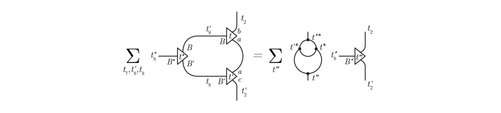
Figure 35: The identity following from eq. (203).

Now we represent the product $E^{b^{\prime},a^{\prime},s;L}_{B;b,a,t}E^{a^{\prime},c^{\prime},s^{\prime};L}_{B^{\prime};a,c,t^{\prime}}$ as the left side of fig. 36.

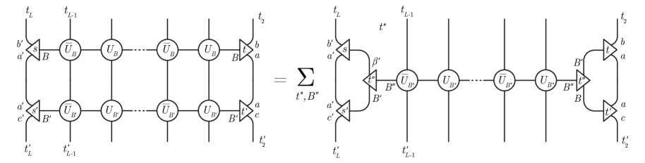
Figure 36: The product $E^{b^{\prime},a^{\prime},s;L}_{B;b,a,t}E^{a^{\prime},c^{\prime},s^{\prime};L}_{B^{\prime};a,c,t^{\prime}}$.

Applying the zipper lemma $L$ times we get the picture on the right side of fig. 36. Then we apply (203) (i.e. fig. 35) at both ends of that picture, and apply the ONB property to the sum over $u$, we get

$$\begin{split}&E^{b^{\prime},a^{\prime},s;L}_{B;b,a,t}E^{a^{\prime},c^{\prime},s^{\prime};L}_{B^{\prime};a,c,t^{\prime}}\\ =&\ \sum_{s^{\prime\prime},t^{\prime\prime}}(d_{a}d_{a^{\prime}})^{1/2}[s^{\prime\prime*}(1_{c^{\prime}}\times r_{a^{\prime}}^{*}\times 1_{\bar{b}^{\prime}})(s^{\prime}\times s)(t^{\prime*}\times t^{*})(1_{c}\times r_{a}\times 1_{\bar{b}})t^{\prime\prime}]E^{c^{\prime},b^{\prime},s^{\prime\prime};L}_{B^{\prime\prime};c,b,t^{\prime\prime}},\end{split}$$ (131)

as described graphically in fig. 37.

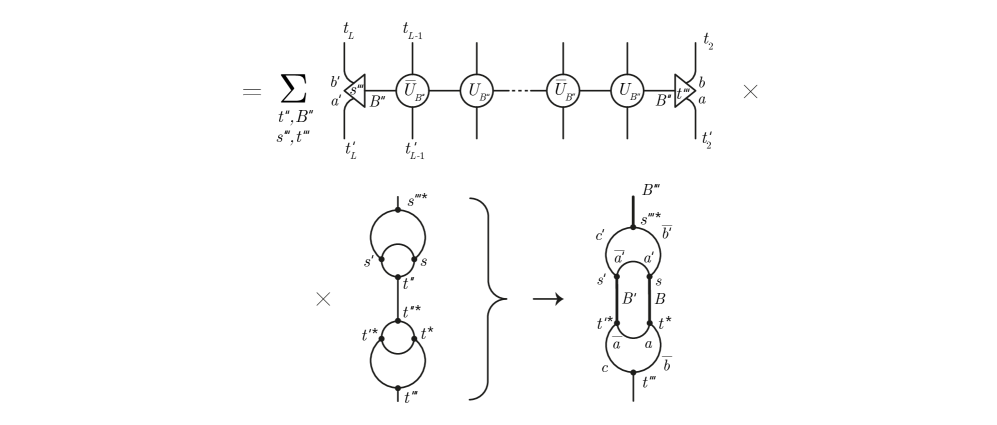
Figure 37: The right side of fig. 36.

This is precisely the multiplication law in the double triangle algebra “when the indices match”, because the scalar $C_{s,t;s^{\prime},t^{\prime}}^{s^{\prime\prime},t^{\prime\prime}}:=(d_{a}d_{a^{\prime}})^{1/2}[\dots]$ on the right side in (131) is the structure constant arising when projecting $e^{b^{\prime},a^{\prime},s}_{B;b,a,t}\star e^{a^{\prime},c^{\prime},s^{\prime}}_{B^{\prime};a,c,t^{\prime}}$ onto the $e^{c^{\prime},b^{\prime},s^{\prime\prime}}_{B^{\prime\prime};c,b,t^{\prime\prime}}$ component, see bottom panel in fig. 36 and fig. 37.

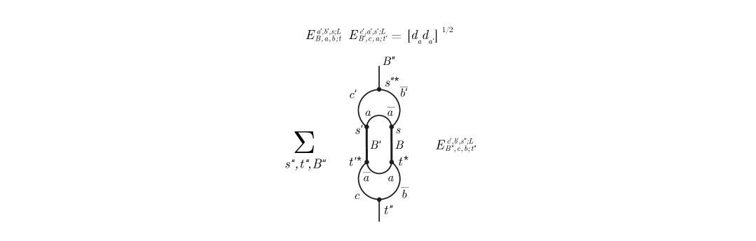
Figure 38: The formula for the product $E^{b^{\prime},a^{\prime},s;L}_{B;b,a,t}E^{a^{\prime},c^{\prime},s^{\prime};L}_{B;a,c,t^{\prime}}$ following from fig. 37.

When the indices do not match, we get zero simply because the intertwiner spaces do not match either. ∎

Recall the definition of $p^{\mp}_{\mu},q_{\mu,\nu}\in{{\cal Z}}_{h}$ [see (87), (89)], where $\mu,\nu\in{}_{{\cal N}}X_{{\cal N}}$. The above representation $\pi^{L}$ gives linear operators

$$Q^{L}_{\mu,\nu}:=\pi^{L}(q_{\mu,\nu})$$ (132)

for any length $L$ of the spin chain. These operators leave the subspace $\mathscr{V}^{L}\subset\mathscr{V}^{L}_{\rm open}$ of periodic spin chain configurations invariant because for elements in ${{\cal Z}}_{h}$, the source and target objects in the corresponding paths $P=(t_{1},\dots,t_{L})\in{\rm Path}_{a^{\prime},a}$ and $P^{\prime}=(t_{1}^{\prime},\dots,t_{L}^{\prime})\in{\rm Path}_{b^{\prime},b}$ are the same, $a=a^{\prime},b=b^{\prime}$. We have the following

Corollary 1.

The following holds for all $L=2k\geq 0$:

1. For $B\in\ _{{\cal M}}X_{{\cal M}}$ we have

   $$\pi^{L}(e_{B})=d_{B}\cdot O_{B}^{L},$$ (133)

   where $O_{B}^{L}$ coincides with the MPOs defined earlier in (107).

2. For $\nu\in\ _{{\cal N}}X_{{\cal N}}$ we have

   $$\pi^{L}(p^{\pm}_{\nu})=d_{\nu}\cdot O_{\alpha_{\nu}^{\pm}}^{L},$$ (134)

   where $O_{A}^{L}$ coincides with the MPOs defined earlier in (107) and $A=\alpha^{\pm}_{\nu}$ are the alpha-induced endomorphisms of ${{\cal M}}$.

3. There holds

   $$O_{\alpha^{\pm}_{\lambda}}=\sum_{B\in\ _{{\cal M}}X_{{\cal M}}}\langle\alpha_{\lambda}^{\pm},B\rangle\,O_{B}$$ (135)

   and we have the fusion

   $$O_{\alpha_{\mu}^{\pm}}^{L}O_{\alpha_{\nu}^{\pm}}^{L}=\sum_{\lambda\in\ _{{\cal N}}X_{{\cal N}}}N_{\mu,\nu}^{\lambda}O_{\alpha_{\lambda}^{\pm}}^{L},$$ (136)

   for all $\lambda,\mu,\nu\in\ _{{\cal N}}X_{{\cal N}}$.

4. We have

   $$Q_{\lambda,\mu}^{L}=\sum_{A}Y_{\lambda,\mu,A}\,O_{A}^{L},$$ (137)

   with $Y_{\lambda,\mu,A}$ as in fig. 27 and (94). $Q^{L}_{\mu,\nu}=0$ iff $Z_{\mu,\nu}=\langle\alpha^{+}_{\mu},\alpha^{-}_{\nu}\rangle=0$, $Q^{L}_{\mu,\nu}=(Q^{L}_{\mu,\nu})^{\dagger}$, $Q_{\mu,\nu}^{L}Q^{L}_{\mu^{\prime},\nu^{\prime}}=\delta_{\mu,\mu^{\prime}}\delta_{\nu,\nu^{\prime}}Q^{L}_{\mu,\nu}$, $[O_{\alpha^{\pm}_{\lambda}}^{L},Q^{L}_{\mu,\nu}]=[O_{B}^{L},Q^{L}_{\mu,\nu}]=0$ for all $\mu,\nu,\lambda\in\ _{{\cal N}}X_{{\cal N}},B\in\ _{{\cal M}}X_{{\cal M}}$.

5. $\sum_{\mu,\nu\in_{{\cal N}}X_{{\cal N}}}Q_{\mu,\nu}^{L}=I^{L}$, where $I^{L}$ is the identity operator (matrix elements $(I^{L})^{P}_{P^{\prime}}=\delta_{P,P^{\prime}}$) on the spin chain.

6. $Q_{0,0}^{L}=P^{L}$, with $P^{L}$ the orthogonal projector given by thm. 1.

7. We have

   $$\sum_{\mu,\lambda\in\,_{{\cal N}}X_{{\cal N}}}\frac{d_{\lambda}d_{\mu}}{D_{X}}O_{\alpha_{\lambda}^{+}}^{L}O_{\alpha_{\mu}^{-}}^{L}=P^{L}$$ (138)

   with $P^{L}$ the orthogonal projector given by thm. 1 and $D_{X}=\sum_{\mu\in\,_{{\cal N}}X_{{\cal N}}}d_{\mu}^{2}$.

Proof.

1) The is similar to 2) but simpler and therefore omitted. Note that the claim is consistent with the fusion algebra (85) for $e_{B}$ in the double triangle algebra and theorem 1.

2) For $a,b\in{}_{{\cal M}}X_{{\cal N}},M_{i}\in{}_{{\cal M}}X_{{\cal M}},\lambda,\mu\in{}_{{\cal N}}X_{{\cal N}},$ let $s\in{\mathrm{Hom}}_{{\cal M}}(b\lambda,a),t_{1}\in{\mathrm{Hom}}_{{\cal M}}(\alpha^{\pm}_{\lambda}M_{2},M_{1}),t_{2}\in{\mathrm{Hom}}_{{\cal M}}(b\overline{\imath},M_{2}),t_{3}\in{\mathrm{Hom}}_{{\cal M}}(a\overline{\imath},M_{1})$ be members of ONBs of intertwiners. Now we define

$${}^{\pm}Z_{a,\bar{b}}^{\lambda}\begin{pmatrix}&&t_{2}\\ s;&t_{1}&\\ &&t_{3}\end{pmatrix}:=t_{1}^{*}(\bar{r}_{b}^{*}\times 1_{\alpha_{\lambda}^{\pm}}\times 1_{M_{2}})(1_{b}\times\varepsilon^{\pm}(\lambda,\bar{b})\times t_{2}^{*})(s\times r_{b}\times 1_{\bar{\imath}})t_{3},$$ (139)

see fig. 39. We also define the $Z$ with the rearranged indices used below by complex conjugation of this expression. A simple BF move and the definition of the $6j$-symbols shows that

$${}^{\pm}Z_{a,\bar{b}}^{\lambda}\begin{pmatrix}&t_{2}&\\ s;&&t_{1}\\ &t_{3}&\end{pmatrix}=U_{\alpha^{\pm}_{\lambda}}\begin{pmatrix}&t_{2}&\\ s^{\prime};&&t_{1}\\ &t_{3}&\end{pmatrix}$$ (140)

where $s^{\prime}=\varepsilon^{\pm}(b,\lambda)s$, which defines an intertwiner in ${\mathrm{Hom}}(\alpha^{\pm}_{\lambda}b,a)$. The claim then follows from the definition (107) of the MPOs $O^{L}_{\alpha^{\pm}_{\lambda}}$ and the following lem. 4.

3) These formulas follow from (87), (88) combined with 1), 2) and the fact that $\pi^{L}$ is a representation of the double triangle algebra.

4) The relations for $Q^{L}_{\mu,\nu}$ except the formula for the adjoint follows immediately from the previous theorem and (92). Applying $\pi^{L}$ to (93) and using (93) and item 1) of lem. 2 gives (LABEL:eq:qlm). Then taking the adjoint and using $O_{A}^{\dagger}=O_{A}$ (see thm. 1) as well as item 2) of lem. 2 gives the claim. The commutation relations follow from 1), 2), the fact that the triangle algebra elements $e_{B},p^{\pm}_{\mu}$ are in the horizontal center, and the fact that the $q_{\mu,\nu}$ are the central projections.

5) By [58], thm. 6.8, we have $\sum_{\mu,\nu}q_{\mu,\nu}=e_{0}$, where $e_{0}$ is the projector $e_{B}$ of the double triangle algebra with $B=$ identity morphism. Applying $\pi^{L}$ gives $\sum_{\mu,\nu}Q_{\mu,\nu}^{L}=\pi^{L}(e_{0})$. Therefore, $\pi^{L}(e_{0})$ is equal to $I^{L}$ since $e_{0}$ is the unit of the double triangle algebra. (One can also see using the explicit definition of $\pi^{L}(e_{0})$ in terms of $6j$-symbols.)

6) Evaluating the definition of $q_{\mu,\nu}$ for $\mu=\nu=0=$ identity morphism in the triangle algebra (89) shows that it is equal to $\sum_{B\in\ _{{\cal M}}X_{{\cal M}}}e_{B}=f_{0}$, which is the “horizontal unit” in the double triangle algebra. Applying $\pi^{L}$ and using the definition of $P^{L}$ in theorem 1 gives the result.

7) This follows from 1), 2), 3) together with [58], thm. 5.10. ∎

Lemma 4.

The double triangle elements $p^{\pm}_{\lambda}$ have the MPO representations (where $P,P^{\prime}\in{\rm Path}^{L}_{c}$ and $L=2k$):

$$\begin{split}&\hskip 99.58464pt\pi^{L}(p_{\lambda}^{\pm})^{P}_{P^{\prime}}:=d_{\lambda}\sum_{a,b}\ \sum_{s,s_{1},\dots,s_{L+1}}\cdot\\ &\cdot\ {}^{\pm}Z_{a,\bar{b}}^{\lambda}\begin{pmatrix}&t_{1}&\\ s;&&s_{1}\\ &t_{1}^{\prime}&\end{pmatrix}\prod_{j=1}^{k}\left\{\overline{U}_{\alpha^{\pm}_{\lambda}}\begin{pmatrix}&t_{2j-1}&\\ s_{2j-1}&&s_{2j}\\ &t_{2j-1}^{\prime}&\end{pmatrix}U_{\alpha^{\pm}_{\lambda}}\begin{pmatrix}&t_{2j}&\\ s_{2j}&&s_{2j+1}\\ &t_{2j}^{\prime}&\end{pmatrix}\right\}{}^{\pm}Z_{a,\bar{b}}^{\lambda}\begin{pmatrix}&&t_{L}\\ s;&s_{L+1}&\\ &&t_{L}^{\prime}\end{pmatrix}.\end{split}$$

Proof.

We consider the “$+$” case and denote by $\{v\}$ an ONB of partial isometries of ${\mathrm{Hom}}_{{\cal M}}(\alpha^{+}_{\lambda},B)$, where $B\in{}_{{\cal M}}X_{{\cal M}},\lambda\in{}_{{\cal N}}X_{{\cal N}}$. Thus, $v^{*}v=1$ and $\sum_{v}vv^{*}=1$ in an obvious notation. By definition, this ONB has $\langle B,\alpha_{\lambda}^{+}\rangle$ elements. For $t\in{\mathrm{Hom}}_{{\cal M}}(a\bar{b},B)$, $a,b\in{}_{{\cal N}}X_{{\cal M}}$, we write

$$s_{v,t,B}:=\left[\frac{d_{a}}{d_{B}}\right]^{1/2}\ \varepsilon^{+}(\lambda,b)(v\times 1_{b})(t^{*}\times 1_{b})(1_{a}\times r_{b}),$$ (141)

with $r_{b}$ as usual a solution to the conjugacy relations. It follows that as $t,v$ run through ONBs of intertwiners, $s_{v,t,B}$ runs through an ONB of intertwiners in ${\mathrm{Hom}}_{{\cal M}}(b\lambda,a)$. Letting $v,v^{\prime}$ be two isometries from our ONB of ${\mathrm{Hom}}_{{\cal M}}(\alpha^{+}_{\lambda},B)$ for fixed $B$, the definitions give

$$\left[\frac{d_{a}}{d_{B}}\right]^{-1/2}\ {}^{+}Z_{a,\bar{b}}^{\lambda}\begin{pmatrix}&&t_{0}\\ s_{v,t,B};&u_{v^{\prime}}&\\ &&t_{0}^{\prime}\end{pmatrix}=\delta_{v,v^{\prime}}\ Z_{a,\bar{b}}^{B}\begin{pmatrix}&&t_{0}\\ t;&u&\\ &&t_{0}^{\prime}\end{pmatrix}$$ (142)

where $u\in{\mathrm{Hom}}_{{\cal M}}(BM_{3},M_{1}),t_{0}\in{\mathrm{Hom}}_{{\cal M}}(b\overline{\imath},M_{2}),t_{0}^{\prime}\in{\mathrm{Hom}}_{{\cal M}}(a\overline{\imath},M_{1})$ members of ONBs of intertwiners and $M_{i}\in{}_{{\cal M}}X_{{\cal M}}$. See fig. 39 for the graphical illustration of these formulas.

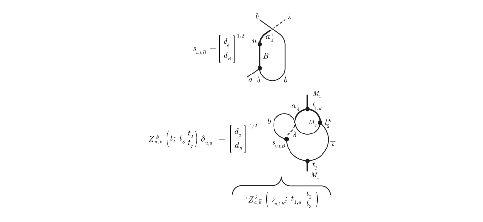
Figure 39: Upper panel: the intertwiner $s_{u,t,B}$. Lower panel: Relationship between ${}^{\pm}Z_{a,\bar{b}}^{\lambda}$ and $Z^{B}_{a,\bar{b}}$.

Here, $u_{v}:=(v\times 1_{M_{3}})u$, which runs through an ONB of intertwiners in ${\mathrm{Hom}}_{{{\cal M}}}(\alpha^{+}_{\lambda}M_{3},M_{1})$ as $v,u$ run through ONBs. We also observe that by construction

$$U_{\alpha^{+}_{\lambda}}\begin{pmatrix}&t_{j}&\\ u_{j,v_{j}}&&u_{j+1,v_{j+1}}\\ &t_{j}^{\prime}&\end{pmatrix}=\delta_{v_{j},v_{j+1}}\ U_{B}\begin{pmatrix}&t_{j}&\\ u_{j}&&u_{j+1}\\ &t_{j}^{\prime}&\end{pmatrix}$$ (143)

for partial isometries $v_{j}$ from our ONB of ${\mathrm{Hom}}_{{\cal M}}(\alpha^{+}_{\lambda},B)$ for fixed $B$. A similar relation holds for the conjugate $6j$-symbol. We make the replacements (142), (143) in each factor the on the right side of the following expression using an ONB of partial isometries $v_{j}\in{\mathrm{Hom}}_{{\cal M}}(\alpha^{+}_{\lambda},B)$ for each $j$ in the defining relation for $\pi^{L}$ multiplied by a Kronecker delta:

$$\begin{split}&\delta_{v,v^{\prime}}\pi^{L}(e_{B;t^{\prime},b^{\prime},a^{\prime}}^{t,b,a})^{P}_{P^{\prime}}=\,[d(a)d(b)d(a^{\prime})d(b^{\prime})]^{1/4}\sum_{u_{1},\dots,u_{L+1}}\sum_{v_{1},\dots,v_{L+1}}\delta_{v,v_{1}}\delta_{v_{1},v_{2}}\cdots\delta_{v_{L},v_{L+1}}\delta_{v_{L+1},v^{\prime}}\cdot\\ &\,Z_{a^{\prime},\bar{b}^{\prime}}^{B}\begin{pmatrix}&t_{1}&\\ t^{\prime};&&u_{1}\\ &t_{1}^{\prime}&\end{pmatrix}\prod_{j=1}^{k}\left\{\overline{U}_{B}\begin{pmatrix}&t_{2j-1}&\\ u_{2j-1}&&u_{2j}\\ &t_{2j-1}^{\prime}&\end{pmatrix}U_{B}\begin{pmatrix}&t_{2j}&\\ u_{2j}&&u_{2j+1}\\ &t_{2j}^{\prime}&\end{pmatrix}\right\}\,Z_{a,\bar{b}}^{B}\begin{pmatrix}&&t_{L}\\ t;&u_{L+1}&\\ &&t_{L}^{\prime}\end{pmatrix}\end{split}$$

and note that the delta-function implies that we can insert an additional summation over the $v_{j}$ in the resulting expression, so that we can subsequently use (143) and (142) on the terms in the product. Then setting $s:=s_{v,t,B},s^{\prime}=s_{v^{\prime},t^{\prime},B}$ resp. $s_{j}=u_{j,v_{j}}$ we obtain an equivalent sum over an ONB of intertwiners in ${\mathrm{Hom}}_{{\cal M}}(b\lambda,a)$ resp ${\mathrm{Hom}}_{{{\cal M}}}(\alpha^{+}_{\lambda}M_{j},M_{j}^{\prime})$. In the resulting equality we set $v=v^{\prime},a=a^{\prime},b=b^{\prime},s=s^{\prime}$. The left side of the equality no longer depends on $v$, so if we perform a summation over $v\in{\mathrm{Hom}}_{{\cal M}}(\alpha^{+}_{\lambda},B)$ for fixed $B$, we obtain a factor of $\langle B,\alpha_{\lambda}^{+}\rangle$ on that side. Then we divide by $d_{B}$ and take the sum over $B$ and then $a,b$. This gives among other things a summation over $s,s_{j}$ on the right side. Using the defining equation $e_{B}=\sum_{t,a,b}e_{B;t,b,a}^{t,b,a}$ results in

$$\begin{split}&\hskip 42.67912pt\sum_{B}d_{B}^{-1}\langle B,\alpha_{\lambda}^{+}\rangle\pi^{L}(e_{B})^{P}_{P^{\prime}}=\sum_{a,b}\sum_{s,s_{1},\dots,s_{L+1}}\cdot\\ &\cdot\ {}^{+}Z_{a,\bar{b}}^{\lambda}\begin{pmatrix}&t_{1}&\\ s;&&s_{1}\\ &t_{1}^{\prime}&\end{pmatrix}\prod_{j=1}^{k}\left\{\overline{U}_{\alpha^{+}_{\lambda}}\begin{pmatrix}&t_{2j-1}&\\ s_{2j-1}&&s_{2j}\\ &t_{2j-1}^{\prime}&\end{pmatrix}U_{\alpha^{+}_{\lambda}}\begin{pmatrix}&t_{2j}&\\ s_{2j}&&s_{2j-1}\\ &t_{2j}^{\prime}&\end{pmatrix}\right\}{}^{+}Z_{a,\bar{b}}^{\lambda}\begin{pmatrix}&&t_{L}\\ s;&s_{L+1}&\\ &&t_{L}^{\prime}\end{pmatrix}.\end{split}$$

This is equivalent to the claimed statement using the definition of $\pi^{L}$ and of $p^{\pm}_{\lambda}$ (87). ∎

3.3 Chain Hamiltonians, local operators

Consider a vector $|t_{1},\dots,t_{L}\rangle\in\mathscr{V}^{L}_{\rm open}$. According to the description of such vectors as sequences of compatible intertwiners, this may be interpreted as a specific intertwiner $\in{\mathrm{Hom}}(B(\imath\bar{\imath})^{k},C)$, where $L=2k$. On ${\mathrm{Hom}}(B(\imath\bar{\imath})^{k},C)$ the Jones projections $B(e_{0}),B(e_{-1}),\dots,B(e_{-(L-1)})$ act by left multiplication, so we have an action of the algebra ${{\cal T}}{{\cal L}}_{[0,L-1]}$ generated by these projections on $\mathscr{V}^{L}_{\rm open}$. We call $E^{L}_{x},x=1,\dots,L$ the operator induced by the Jones projection $e_{-(x-1)}$ on $\mathscr{V}^{L}_{\rm open}$. Its matrix elements are

$$\langle t_{1},\dots,t_{L}|E^{L}_{x}|t_{1}^{\prime},\dots,t_{L}^{\prime}\rangle=\begin{cases}[(t_{x}\times 1_{\imath})t_{x+1}]^{*}e_{0}(t_{x}^{\prime}\times 1_{\imath})t_{x+1}^{\prime}&\text{$x$ even,}\\ [(t_{x}\times 1_{\bar{\imath}})t_{x+1}]^{*}e_{-1}(t_{x}^{\prime}\times 1_{\bar{\imath}})t_{x+1}^{\prime}&\text{$x$ odd,}\end{cases}$$ (144)

noting that the expressions are scalars. Using the expressions $e_{0}=d^{-1}\bar{r}\bar{r}^{*},e_{-1}=d^{-1}\bar{\imath}(rr^{*})$ one easily finds the numerical value of the matrix elements to be

$$\begin{split}&\langle t_{1},\dots,t_{L}|E^{L}_{x}|t_{1}^{\prime},\dots,t_{L}^{\prime}\rangle\\ =&d^{-1}(t_{x+1}^{\prime},\tilde{t}_{x}^{\prime})(\tilde{t}_{x+1},t_{x})\begin{cases}\left(\frac{d(M_{x}^{\prime})d(M_{x})}{d(a_{x}^{\prime})d(a_{x})}\right)^{1/2}\delta_{a_{x},a_{x+1}}\delta_{a_{x}^{\prime},a_{x+1}^{\prime}}&\text{$x$ even,}\\ \left(\frac{d(a_{x}^{\prime})d(a_{x})}{d(M_{x}^{\prime})d(M_{x})}\right)^{1/2}\delta_{M_{x},M_{x+1}}\delta_{M_{x}^{\prime},M_{x+1}^{\prime}}&\text{$x$ odd,}\end{cases}\end{split}$$ (145)

where the intertwiners are supposed to be from the spaces $t_{x}\in{\mathrm{Hom}}(a_{x}\bar{\imath},M_{x}),t_{x+1}\in{\mathrm{Hom}}(M_{x}\imath,a_{x+1})$ (and similarly $t_{x}^{\prime},t_{x+1}^{\prime}$) when $x$ is even and from $t_{x}\in{\mathrm{Hom}}(M_{x}\imath,a_{x}),t_{x+1}\in{\mathrm{Hom}}(a_{x}\bar{\imath},M_{x+1})$ (and similarly $t_{x}^{\prime},t_{x+1}^{\prime}$) when $x$ is odd. The inner products $(\tilde{t}_{x+1},t_{x})$ or $(t_{x+1}^{\prime},\tilde{t}_{x}^{\prime})$ are as in (20) and “tilde” means the Frobenius dual of an intertwiner, see (24).

By construction, the $E^{L}_{x}$ are projections. We denote by

$${{\cal T}}{{\cal L}}_{[x_{1},x_{2}]}^{L}:=\text{algebra generated by $E_{x}^{L},x_{1}<x<x_{2}-1$,}$$ (146)

the algebra of local operators acting on the sites $x_{1},x_{1}+1,\dots,x_{2}$. By construction, these algebras are isomorphic to Temperly-Lieb-Jones algebras with $x_{2}-x_{1}-1$ generators and parameter $d$. We have the following Lemma.

Lemma 5.

Any element $A\in{{\cal T}}{{\cal L}}_{[2,L-1]}^{L}$ commutes with any MPO in $\pi^{L}(\lozenge)$, i.e. with the image of the double triangle algebra under the representation $\pi^{L}$ on $\mathscr{V}^{L}_{\rm open}$.

Proof.

We may write the projectors $E_{x}^{L}$ in terms of $6j$-symbols as in [20]. Then we can see that we can move $E_{x}^{L}$ at any point through the chain of $U_{B},\bar{U}_{B}$’s as in fig. 33 using a “vertical” version of the zipper lemma, which is proven in exactly the same way as the zipper lemma itself.

With a certain amount of tedium, one can also show this directly without a graphical notation which we do here since we have not demonstrated the vertical zipper lemma. For definiteness, take $x$ even (the other case is similar). At the level of matrix elements, the proof boils down to the statement that

$$\begin{split}&\sum_{t,t^{\prime}_{x},t^{\prime}_{x+1}}U_{B}\left(\begin{matrix}&t^{\prime}_{x}&\\ s_{1}&&t\\ &t_{x}&\end{matrix}\right)\bar{U}_{B}\left(\begin{matrix}&t^{\prime}_{x+1}&\\ t&&s_{2}\\ &t_{x+1}&\end{matrix}\right)\langle\dots t^{\prime\prime}_{x},t^{\prime\prime}_{x+1}\dots|E^{L}_{x}|\dots t^{\prime}_{x},t^{\prime}_{x+1}\dots\rangle\\ =&\sum_{t,t^{\prime}_{x},t^{\prime}_{x+1}}U_{B}\left(\begin{matrix}&t^{\prime\prime}_{x}&\\ s_{1}&&t\\ &t^{\prime}_{x}&\end{matrix}\right)\bar{U}_{B}\left(\begin{matrix}&t^{\prime\prime}_{x+1}&\\ t&&s_{2}\\ &t^{\prime}_{x+1}&\end{matrix}\right)\langle\dots t^{\prime}_{x},t^{\prime}_{x+1}\dots|E^{L}_{x}|\dots t_{x},t_{x+1}\dots\rangle\end{split}$$ (147)

where the intertwiners are supposed to be from the spaces $t_{x}\in{\mathrm{Hom}}(a_{x}\bar{\imath},M_{x}),t_{x+1}\in{\mathrm{Hom}}(M_{x}\imath,a_{x+1}),t_{x}^{\prime}\in{\mathrm{Hom}}(a_{x}^{\prime}\bar{\imath},M_{x}^{\prime}),t_{x+1}^{\prime}\in{\mathrm{Hom}}(M_{x}^{\prime}\imath,a_{x+1}^{\prime})t_{x}\in{\mathrm{Hom}}(a_{x}^{\prime\prime}\bar{\imath},M_{x}^{\prime\prime}),t_{x+1}^{\prime\prime}\in{\mathrm{Hom}}(M_{x}^{\prime\prime}\imath,a_{x+1}^{\prime\prime})$, as well as $s_{1}\in{\mathrm{Hom}}(Ba_{x}^{\prime},a_{x}),s_{2}\in{\mathrm{Hom}}(Ba^{\prime}_{x+1},a_{x+1}),t\in{\mathrm{Hom}}(BM_{x}^{\prime},M_{x})$. Only two $6j$-symbols are involved because $E_{x}^{L}$ only acts non-trivially on the sites $x,x+1$. We now evaluate the left side of (147) making use of the intertwiner calculus, the definitions of the $6j$-symbols, of (144), and of $e_{0}=d^{-1}\bar{r}\bar{r}^{*}$:

$$\begin{split}=&d^{-1}(\tilde{t}_{x+1}^{\prime\prime},t_{x}^{\prime\prime})\left(\frac{d(M_{x}^{\prime\prime})}{d(a_{x}^{\prime\prime})}\right)^{1/2}\delta_{a_{x}^{\prime\prime},a_{x+1}^{\prime\prime}}\sum_{t,t^{\prime}_{x},t^{\prime}_{x+1}}\\ &t^{\prime*}_{x}(1_{\bar{\imath}}\times t^{\prime*}_{x+1})(\bar{r}\times 1_{a^{\prime}_{x+1}})\ t_{x}^{*}(s_{1}^{*}\times 1_{\bar{\imath}})(1_{B}\times t_{x}^{\prime})t\ t_{x+1}^{*}(t^{*}\times 1_{\imath})(1_{B}\times t^{\prime}_{x+1})s_{2}\\ =&d^{-1}(\tilde{t}_{x+1}^{\prime\prime},t_{x}^{\prime\prime})\left(\frac{d(M_{x}^{\prime\prime})}{d(a_{x}^{\prime\prime})}\right)^{1/2}\delta_{a_{x}^{\prime\prime},a_{x+1}^{\prime\prime}}\sum_{t^{\prime}_{x},t^{\prime}_{x+1}}\delta_{a_{x}^{\prime},a_{x+1}^{\prime}}\\ &t^{\prime*}_{x}(1_{\bar{\imath}}\times t^{\prime*}_{x+1})(\bar{r}\times 1_{a^{\prime}_{x}})\ t_{x+1}^{*}(t_{x}^{*}\times 1_{\imath})(s_{1}^{*}\times 1_{\bar{\imath}\imath})(1_{B}\times t_{x}^{\prime}\times 1_{\imath})(1_{B}\times t^{\prime}_{x+1})s_{2}\\ =&d^{-1}(\tilde{t}_{x+1}^{\prime\prime},t_{x}^{\prime\prime})\left(\frac{d(M_{x}^{\prime\prime})}{d(a_{x}^{\prime\prime})}\right)^{1/2}\delta_{a_{x}^{\prime\prime},a_{x+1}^{\prime\prime}}\sum_{t^{\prime}_{x}}\delta_{a_{x}^{\prime},a_{x+1}^{\prime}}\\ &t^{\prime*}_{x}(1_{\bar{\imath}}\times t^{\prime*}_{x+1})(s_{1}^{*}\times 1_{\bar{\imath}\imath})(1_{B}\times t_{x}^{\prime}\times 1_{\imath})(1_{B}\times t_{x}^{\prime*}\times 1_{\imath})(s_{2}\times\bar{r})\\ =&d^{-1}(\tilde{t}_{x+1}^{\prime\prime},t_{x}^{\prime\prime})(\tilde{t}_{x+1},t_{x})\left(\frac{d(M_{x}^{\prime\prime})d(M_{x})}{d(a_{x}^{\prime\prime})d(a_{x})}\right)^{1/2}\delta_{a_{x}^{\prime\prime},a_{x+1}^{\prime\prime}}\delta_{a_{x},a_{x+1}}\delta_{s_{1},s_{2}}\end{split}$$ (148)

We proceed in a similar manner evaluating the right side of (147),

$$\begin{split}=&d^{-1}(\tilde{t}_{x+1},t_{x})\left(\frac{d(M_{x})}{d(a_{x})}\right)^{1/2}\delta_{a_{x},a_{x+1}}\sum_{t,t^{\prime}_{x},t^{\prime}_{x+1}}\\ &(1_{a_{x}^{\prime}}\times\bar{r}^{*})(t_{x}^{\prime}\times 1_{\imath})t_{x+1}^{\prime}\ t^{\prime*}_{x}(s_{1}^{*}\times 1_{\imath})(1_{B}\times t_{x}^{\prime\prime})t\ t^{\prime*}_{x+1}(t^{*}\times 1_{\imath})(1_{B}\times t_{x+1}^{\prime\prime})s_{2}\\ \\ =&d^{-1}(\tilde{t}_{x+1},t_{x})\left(\frac{d(M_{x})}{d(a_{x})}\right)^{1/2}\delta_{a_{x},a_{x+1}}\sum_{t^{\prime}_{x},t^{\prime}_{x+1}}\delta_{a_{x}^{\prime},a_{x+1}^{\prime}}\\ &t^{\prime*}_{x+1}(t^{\prime*}_{x}\times 1_{\imath})(s_{1}^{*}\times 1_{\bar{\imath}\imath})(1_{B}\times t_{x}^{\prime\prime}\times 1_{\imath})(1_{B}\times t_{x+1}^{\prime\prime})s_{2}\ (1_{a_{x}^{\prime}}\times\bar{r}^{*})(t_{x}^{\prime}\times 1_{\imath})t^{\prime}_{x+1}\\ =&d^{-1}(\tilde{t}_{x+1},t_{x})\left(\frac{d(M_{x})}{d(a_{x})}\right)^{1/2}\delta_{a_{x},a_{x+1}}(s_{1}^{*}\times\bar{r}^{*})(1_{B}\times t_{x}^{\prime\prime}\times 1_{\imath})(1_{B}\times t_{x+1}^{\prime\prime})s_{2}\\ =&d^{-1}(\tilde{t}_{x+1}^{\prime\prime},t_{x}^{\prime\prime})(\tilde{t}_{x+1},t_{x})\left(\frac{d(M_{x}^{\prime\prime})d(M_{x})}{d(a_{x}^{\prime\prime})d(a_{x})}\right)^{1/2}\delta_{a_{x}^{\prime\prime},a_{x+1}^{\prime\prime}}\delta_{a_{x},a_{x+1}}\delta_{s_{1},s_{2}}\end{split}$$ (149)

which is the same as before and thus concludes the proof. ∎

We mention that for a closed spin chain (i.e. a state in $\mathscr{V}^{L}$), we may also construct a Temperly-Lieb projection $E_{x}^{L}$ for $x=L$ which we think of as involving the sites $1$ and $L$ at least in certain cases. In the literature, the resulting algebra is called the “annular Temperly-Lieb algebra” [71]. Assume that the Jones index $d^{2}=[{{\cal M}}:{{\cal N}}]<4$. If $\omega:=ie^{i\pi/(2(k+2))},k=1,2,3\dots$, then $d=-(\omega^{2}+\omega^{-2})$ are precisely the possible values of the square root of the Jones index below $2$ (4). It is standard to show that $B_{x}^{L}:=\omega I^{L}+d\omega^{-1}E_{x}^{L},x=1,\dots,L-1$ give a unitary representation of the braid group on $L$ strands. Now define the projection (see fig. 40)

$$E_{L}^{L}=\left(\prod_{x=L-1}^{1}(B_{x}^{L})^{-1}\right)E_{L-1}^{L}\left(\prod_{x=1}^{L-1}B_{x}^{L}\right)$$ (150)

on the closed spin chain. Then $E^{L}_{L}$ is a projection and we have the additional relations $E_{1}^{L}E_{L}^{L}E_{1}^{L}=d^{-1}E_{1}^{L},E_{L-1}^{L}E_{L}^{L}E_{L-1}^{L}=d^{-1}E_{L-1}^{L},E_{L}^{L}E_{1}^{L}E_{L}^{L}=d^{-1}E^{L}_{L},[E^{L}_{x},E^{L}_{L}]=0\,(|x-L|>1)$ of the annular Temperly-Lieb algebra (using the opposite braiding $(B_{x}^{L})^{-1}$ gives another representation.)

Figure 40: Wire diagram for the MPO $E^{L}_{L}$. The crossings represent $B_{x}^{L}:=\omega I^{L}+d\omega^{-1}E_{x}^{L}$.

For the open (closed) spin chain, we define the Hamiltonian as

$$H:=J\sum_{x=1}^{L-1}E_{x}^{L}\quad(+JE^{L}_{L}),$$ (151)

where $J$ is a coupling constant. By the previous lemma and cor. 1, we have $[O_{A}^{L},E^{L}_{x}]=[Q_{\lambda,\mu}^{L},E^{L}_{x}]=0$ for all $x\in[1,L]$ for the closed chain or all $x\in[1,L-1]$ for the open chain. In either case we get, noting that $Q_{\lambda,\mu}^{L}$ leave the Hilbert space $\mathscr{V}^{L}$ of the closed chain invariant:

Corollary 2.

The local densities $E_{x}^{L}$ of the Hamiltonian leave the “sectors” $\mathscr{V}_{\lambda,\mu}^{L}:=Q^{L}_{\lambda,\mu}\mathscr{V}^{L}\subset\mathscr{V}^{L}$ invariant. The same holds for the open chain.

Because the $Q^{L}_{\lambda,\mu}$ are non-zero mutually orthogonal projections whenever $Z_{\lambda,\mu}\neq 0$ (cor. 1), it follows that we have a corresponding direct sum decomposition of the closed chain Hilbert space $\mathscr{V}^{L}$ into the sectors $\mathscr{V}_{\lambda,\mu}^{L}$, each of which is invariant under time evolution and local densities of the Hamiltonian. This is analogous to the case of a rational $1+1$-dimensional CFT, where the sectors of the total Hilbert space splits into sectors labelled by pairs of simple objects $(\lambda,\mu)$ – which are Virasoro-irreps in that case and correspond to the decomposition of the partition function into $\sum_{\lambda,\mu}Z_{\lambda,\mu}\chi_{\lambda}(q)\overline{\chi_{\mu}(q)}$ – each of which is invariant under the densities of the Hamiltonian (Virasoro algebra).

4 Defects

4.1 Defect algebra

In this section, we come to the main results of this paper which concern defects. A defect is roughly a kind of “boundary condition” for a bi-partite closed spin-chain. In our approach, each defect corresponds to an appropriately defined orthogonal summand of the Hilbert space for the full bipartite chain, and is invariant under any local operator as defined in sec. 3.3 which is not acting on the boundary points separating the sub-chains. As we will see, our “boundary conditions” are very similar to the classification of transparent boundaries in 1+1 CFTs, see sec. 2.10, which is in fact the prime motivation for our construction. The subspaces corresponding to the defects are the eigenspaces of an abelian algebra, ${{\cal D}}^{L_{1},L_{2}}$, generated by certain operators $\Psi^{L_{1},L_{2}}_{\nu,\rho;w_{1},w_{2}}$ soldering the two subchains of lengths $L_{1},L_{2}$ together.

Since the defects “sit” where the two sub-chains meet at some time zero snapshot of the chain, we think of them as “vertical” and they would remain in a fixed position if the chain was evolved with a Hamiltonian $H^{L_{1}}+H^{L_{2}}$ which is a sum of a Hamiltonian made from local operators of subchain 1 and 2 which do not touch the endpoints of the subchains. The operators $O_{A}^{L}$ associated with a single chain (see thm. 1) are also often discussed in the literature in connection with defects. We tend to think of them as “horizontal”. The algebra of vertical and horizontal defects turns out to be isomorphic to the fusion algebra ${}_{{\cal M}}X_{{{\cal M}}}$ with structure constants $N_{A,B}^{C}$ in the case of diagonal theories, (see sec. 4.3) although they of course correspond to entirely different representations of that algebra. In the general case, the algebras seem to be non-isomorphic leaving the need for further investigations. Defects from the point of view of PEPs are discussed in app. B, but also here the precise connection needs clarification.

After these preliminaries, we now come the definition of the MPOs $\Psi^{L_{1},L_{2}}_{\nu,\rho;w_{1},w_{2}}$ and their structural properties. The operators $\Psi^{L_{1},L_{2}}_{\nu,\rho;w_{1},w_{2}}$ act on the tensor product of two open chains, i.e. the Hilbert space

$$\mathscr{V}^{L_{1},L_{2}}:=\mathscr{V}^{L_{1}}_{\rm open}\otimes\mathscr{V}^{L_{2}}_{\rm open}.$$ (152)

However, they couple the two tensor copies together at the end-points in each of the chains and therefore connect the two systems. These operators generate the algebra ${{\cal D}}^{L_{1},L_{2}}$ and will be labelled by a pair $\nu,\rho\in\,_{{{\cal N}}}X_{{\cal N}}$ and a pair $w_{1}\in{\mathrm{Hom}}(\alpha_{\nu}^{-},\alpha_{\rho}^{+}),w_{2}\in{\mathrm{Hom}}(\alpha_{\rho}^{+},\alpha_{\nu}^{-})$, so that both $w_{1},w_{2}$ may be thought of as running between $1,\dots,Z_{\rho,\nu}$. The operators will only be defined for pairs $(\nu,\rho)$ such that $Z_{\rho,\nu}\neq 0$, so there are

$$\sum_{\nu,\rho\in\,_{{\cal N}}X_{{\cal N}}}Z_{\nu,\rho}^{2}=|\,_{{\cal M}}X_{{\cal M}}\,|$$ (153)

such operators, using [58], cor. 6.10 in the equality sign. This suggests that the joint eigenspaces of the $\Psi^{L_{1},L_{2}}_{\nu,\rho;w_{1},w_{2}}$ and the central projections of ${{\cal D}}^{L_{1},L_{2}}$ are labelled by the objects $A$ of $\,{}_{{\cal M}}X_{{\cal M}}$, as we will confirm below.

To start, we consider the projection operators $Q^{L_{1}}_{\mu_{1},\lambda_{1}}$ and $Q^{L_{2}}_{\mu_{2},\lambda_{2}}$ and according to our cor. 1, item 5), we can decompose the Hilbert space $\mathscr{V}^{L_{1},L_{2}}$ of the full bipartite chain into an orthogonal direct sum with summands given by

$$\mathscr{V}_{\mu_{1},\lambda_{1};\mu_{2},\lambda_{2}}^{L_{1},L_{2}}:=Q^{L_{1}}_{\mu_{1},\lambda_{1}}\mathscr{V}^{L_{1}}_{\rm open}\otimes Q^{L_{2}}_{\mu_{1},\lambda_{2}}\mathscr{V}^{L_{2}}_{\rm open}.$$ (154)

The operators $\Psi^{L_{1},L_{2}}_{\nu,\rho;w_{1},w_{2}}$ will be engineered to have the following properties:

1. (Identity) For $(\nu,\rho)=(id,id)$ the identity endomorphisms, we have

   $$\Psi^{L_{1},L_{2}}_{id,id;1,1}=I^{L_{1}}\otimes I^{L_{2}},$$ (155)

   where $1$ is the only unitary intertwiner in ${\mathrm{Hom}}(\alpha^{+}_{id},\alpha^{-}_{id})={\mathrm{Hom}}(id,id)={\mathbb{C}}1$ and $I^{L_{i}}$ is the identity operator on the closed chain $\mathscr{V}^{L_{i}}$ (viewed as a projection operator on the open chain Hilbert space).

2. (Conjugate) We have

   $$(\Psi^{L_{1},L_{2}}_{\nu,\rho;w_{1},w_{2}})^{\dagger}=\Psi^{L_{1},L_{2}}_{\nu,\rho;w_{2}^{*},w_{1}^{*}}.$$ (156)

3. (Commutativity) We have

   $$[\Psi^{L_{1},L_{2}}_{\nu,\rho;w_{1},w_{2}},\Psi^{L_{1},L_{2}}_{\nu^{\prime},\rho^{\prime};w_{1}^{\prime},w_{2}^{\prime}}]=0.$$ (157)

   If $A\in{{\cal T}}{{\cal L}}^{L_{1}}_{[2,L_{1}-1]}\otimes{{\cal T}}{{\cal L}}^{L_{2}}_{[2,L_{2}-1]}$ is any local operator on the doubled chain Hilbert space $\mathscr{V}^{L_{1},L_{2}}=\mathscr{V}^{L_{1}}_{\rm open}\otimes\mathscr{V}^{L_{1}}_{\rm open}$ acting on any sites of chain 1 or chain 2 except for the endpoints $\{1,L_{i}\}$ of either chain, then

   $$[\Psi^{L_{1},L_{2}}_{\nu,\rho;w_{1},w_{2}},A]=0.$$ (158)

4. (OPE) We have

   $$\Psi^{L_{1},L_{2}}_{\nu,\rho;w_{1},w_{2}}\Psi^{L_{1},L_{2}}_{\nu^{\prime},\rho^{\prime};w_{1}^{\prime},w_{2}^{\prime}}=\sum_{\nu^{\prime\prime},\rho^{\prime\prime},w_{1}^{\prime\prime},w_{2}^{\prime\prime}}c^{\nu^{\prime\prime},\rho^{\prime\prime},w_{1}^{\prime\prime},w_{2}^{\prime\prime}}_{\nu^{\prime},\rho^{\prime},w_{1}^{\prime},w_{2}^{\prime};\nu,\rho;w_{1},w_{2}}\Psi^{L_{1},L_{2}}_{\nu^{\prime\prime},\rho^{\prime\prime};w_{1}^{\prime\prime},w_{2}^{\prime\prime}}$$ (159)

   where only such terms occur in the sum for which $\nu^{\prime\prime}\subset\nu\nu^{\prime},\rho^{\prime\prime}\subset\rho\rho^{\prime}$, i.e. which are compatible with fusion and. The numerical coefficients are defined as

   $$c^{\nu^{\prime\prime},\rho^{\prime\prime},w_{1}^{\prime\prime},w_{2}^{\prime\prime}}_{\nu^{\prime},\rho^{\prime},w_{1}^{\prime},w_{2}^{\prime};\nu,\rho;w_{1},w_{2}}:=\sum_{e,f}\eta^{w_{1}^{\prime\prime}}_{e,f;w_{1},w_{1}^{\prime}}\eta^{w_{2}^{\prime\prime}}_{f^{*},e^{*};w_{2},w_{2}^{\prime}}$$ (160)

   where $e,f$ run over ONBs of ${\mathrm{Hom}}(\nu\nu^{\prime},\nu^{\prime\prime})$ respectively ${\mathrm{Hom}}(\rho\rho^{\prime},\rho^{\prime\prime})$, and where $\eta^{w^{\prime\prime}}_{e,f;w,w^{\prime}}$ are Rehren’s structure constants (102).

5. (Fusion)

   $$\Psi^{L_{1},L_{2}}_{\nu,\rho;w_{1},w_{2}}\mathscr{V}^{L_{1},L_{2}}_{\lambda_{1},\mu_{1};\lambda_{2},\mu_{2}}\subset\bigoplus_{\lambda_{1}^{\prime},\mu_{1}^{\prime};\lambda_{2}^{\prime},\mu_{2}^{\prime}}\mathscr{V}^{L_{1},L_{2}}_{\lambda_{1}^{\prime},\mu_{1}^{\prime};\lambda_{2}^{\prime},\mu_{2}^{\prime}},$$ (161)

   where only such terms occur in the sum which have $\mu_{i}^{\prime}\subset\nu\mu_{i},\lambda_{i}^{\prime}\subset\rho\lambda_{i}$, i.e. which are compatible with fusion.

We now define the operators $\Psi^{L_{1},L_{2}}_{\nu,\rho;w_{1},w_{2}}$. We denote by $e_{i}$ respectively $f_{i}$ ONBs of

$$e_{1} \in{\mathrm{Hom}}(\mu_{1}\nu,\mu_{1}^{\prime})$$ (162)

$$f_{1} \in{\mathrm{Hom}}(\rho\lambda_{1},\lambda_{1}^{\prime})$$ (163)

$$e_{2} \in{\mathrm{Hom}}(\mu_{2}\rho,\mu_{2}^{\prime})$$ (164)

$$f_{2} \in{\mathrm{Hom}}(\nu\lambda_{2},\lambda_{2}^{\prime}),$$ (165)

where here and in the rest of this section, $i=1,2$ refers to the different subsystems of the bipartite periodic chain. Then we define MPOs $X_{e_{1},f_{2};s,t}^{s^{\prime},t^{\prime}}$ and $X_{e_{2},f_{1};s,t}^{s^{\prime},t^{\prime}}$ acting on two adjacent sites in the chain as in fig. 41, where the down and right pointing triangles denote $6j$-symbols defined by figs. 42 and 43.

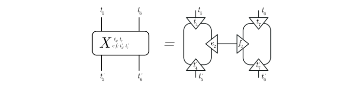
Figure 41: The definition of $X_{e_{1},f_{2};s,t}^{s^{\prime},t^{\prime}}$.

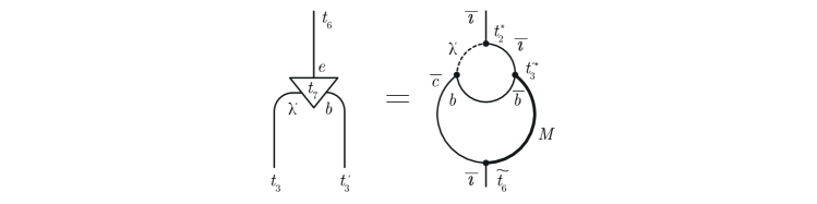
Figure 42: Downwards-pointing triangles.

Figure 43: Leftwards-pointing triangles.

These figures also implicitly define the intertwiner spaces associated with the indices of these MPOs. The up- and left-pointing triangles are defined as their complex conjugates. Next, we let $a,b,c,d\in\,_{{\cal M}}X_{{\cal N}}$, $\mu,\lambda\in\,_{{\cal N}}X_{{\cal N}}$, $t\in{\mathrm{Hom}}(\lambda c,b),s\in{\mathrm{Hom}}(c\mu,d),v\in{\mathrm{Hom}}(\alpha^{-}_{\mu},\alpha^{+}_{\lambda})$ and put

$$\bar{x}_{t,s,v,a}:=(d_{\mu}d_{\lambda})^{1/4}\left(\frac{d_{a}}{d_{c}D_{X}}\right)^{1/2}\,(s^{*}\times 1_{a})(1_{c}\times\varepsilon^{-}(\mu,\bar{a})^{*})(1_{c\bar{a}}\times v)(1_{c}\times\varepsilon^{+}(\lambda,\bar{a}))(t\times 1_{\bar{a}})\quad\in\lozenge,$$ (166)

and then

$$\Phi_{t,s,v}^{L}:=\sum_{a\in\,_{{\cal N}}X_{{\cal N}}}\pi^{L}(\bar{x}_{t,s,v,a}).$$ (167)

This definition is illustrated in the upper box of fig. 44 which also shows in the lower box a graphical illustration of the adjoint. Note that the intertwiner $x_{t,s,v,a}\in\lozenge$ is depicted following the conventions by [58], i.e. its graphical representation as a wire diagram is rotated by 90 degrees relative to our normal conventions for pictures. The formula for the adjoint is

$$(\Phi_{t,s,v}^{L})^{\dagger}:=\sum_{a\in\,_{{\cal N}}X_{{\cal N}}}\pi^{L}(x_{t,s,v,a}),$$ (168)

wherein

$$x_{t,s,v,a}:=(d_{\mu}d_{\lambda})^{1/4}\left(\frac{d_{a}}{d_{c}D_{X}}\right)^{1/2}\,(1_{a}\times\bar{s}^{*})(\varepsilon^{-}(a,\bar{\mu})^{*}\times 1_{c})(\bar{v}\times 1_{a\bar{c}})(\varepsilon^{+}(a,\bar{\lambda})\times 1_{\bar{c}})(1_{a}\times\bar{t})\quad\in\lozenge.$$ (169)

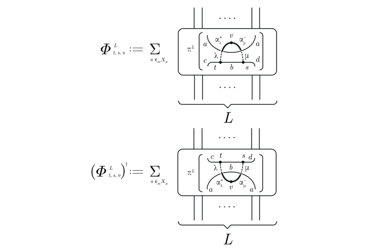
Figure 44: The definition of $\Phi_{t,s,v}^{L}$.

Next, we set

$$\begin{split}\zeta_{e_{1},f_{1};w_{1}v_{1}}^{v_{1}^{\prime}}&:=\left[\frac{d(\mu_{1})d(\nu)}{d(\mu_{1}^{\prime})d(\theta)}\right]^{1/2}E[e^{*}_{1}\varepsilon^{-}(\mu_{1},\nu)^{*}(w_{1}\times v_{1})f_{1}(v_{1}^{\prime})^{*}]\\ \zeta_{e_{2},f_{2};w_{2}v_{2}}^{v_{2}^{\prime}}&:=\left[\frac{d(\mu_{2})d(\rho)}{d(\mu_{2}^{\prime})d(\theta)}\right]^{1/2}E[e^{*}_{2}\varepsilon^{-}(\mu_{2},\rho)^{*}(w_{2}\times v_{2})f_{2}(v_{2}^{\prime})^{*}]\end{split}$$ (170)

with $v_{i}\in{\mathrm{Hom}}(\alpha^{-}_{\mu_{i}},\alpha^{+}_{\lambda_{i}}),v_{i}\in{\mathrm{Hom}}(\alpha^{-}_{\mu_{i}^{\prime}},\alpha^{+}_{\lambda_{i}^{\prime}})$ and $w_{i}$ as above, see fig. 45. Note the similarity to Rehren’s structure constants (102) $\eta_{e_{2},f_{2};w_{2},v_{2}}^{v_{2}^{\prime}}$ which differ only by the braiding operators.

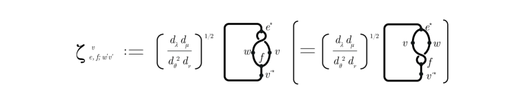
Figure 45: Wire diagram for the $\zeta$-structure constants (170).

Definition 5.

We define the following MPO’s on $\mathscr{V}^{L_{1},L_{2}}$:

$$\begin{split}&\Psi^{L_{1},L_{2}}_{\nu,\rho;w_{1},w_{2}}:=\sum_{t_{i},t_{i}^{\prime},s_{i},s_{i}^{\prime},e_{i},f_{i},v_{i},v_{i}^{\prime}}\zeta_{e_{1},f_{1};w_{1},v_{1}}^{v_{1}^{\prime}}\zeta_{e_{2},f_{2};w_{2},v_{2}}^{v_{2}^{\prime}}\cdot\\ &(\Phi^{L_{1}}_{t_{1},s_{1},v_{1}}\otimes\Phi^{L_{2}}_{t_{2},s_{2},v_{2}})(X^{s_{2},t_{1}}_{e_{2},f_{1};s_{2}^{\prime},t_{1}^{\prime}}\otimes I^{L_{1}-2}\otimes X^{s_{1},t_{2}}_{e_{1},f_{2};s_{1}^{\prime},t_{2}^{\prime}}\otimes I^{L_{2}-2})(\Phi^{L_{1}}_{t_{1}^{\prime},s_{1}^{\prime},v_{1}^{\prime}}\otimes\Phi^{L_{2}}_{t_{2}^{\prime},s_{2}^{\prime},v_{2}^{\prime}})^{\dagger},\end{split}$$ (171)

This definition is illustrated in fig. 46.

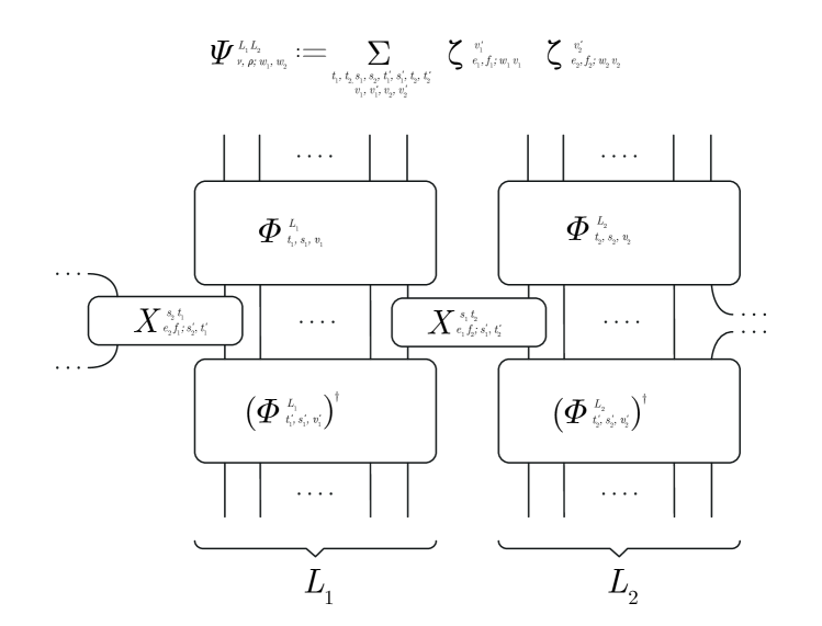
Figure 46: Definition of the MPOs $\Psi^{L_{1},L_{2}}_{\nu,\rho;w_{1},w_{2}}$.

The sums run over ONBs of intertwiners $e_{i},f_{i}$ as in (162) for fixed $\nu,\rho$ and $w_{i}$ and over ONBs

$$\begin{split}&t_{i}\in{\mathrm{Hom}}(\lambda_{i}\bar{b}_{i},\bar{c}_{i}),\quad s_{i}\in{\mathrm{Hom}}(\mu_{i}\bar{b}_{i},\bar{d}_{i}),\\ &t_{i}^{\prime}\in{\mathrm{Hom}}(\lambda_{i}^{\prime}\bar{b}_{i}^{\prime},\bar{c}_{i}^{\prime}),\quad s_{i}^{\prime}\in{\mathrm{Hom}}(\mu_{i}^{\prime}\bar{b}_{i}^{\prime},\bar{d}_{i}^{\prime}).\end{split}$$ (172)

Definition 6.

We define the defect algebra ${{\cal D}}^{L_{1},L_{2}}$ to be the $\dagger-$ algebra generated by the operators $\Psi^{L_{1},L_{2}}_{\nu,\rho;w_{1},w_{2}}$.

The following is one of the main results of this paper and clarifies the nature of the defect algebra.

Theorem 3.

The MPOs $\Psi_{\nu,\rho;w_{1},w_{2}}^{L_{1},L_{2}}$ as in def. 5 fulfill properties 1)–5).

Proof.

1) In this case $f_{i}=e_{i}=1$ and consequently $X^{s_{2},t_{1}}_{e_{2},f_{1};s_{2}^{\prime},t_{1}^{\prime}}=\delta^{s_{2}}_{s_{2}^{\prime}}\delta^{t_{1}}_{t_{1}^{\prime}}$ and $X^{s_{1},t_{2}}_{e_{1},f_{2};s_{1}^{\prime},t_{2}^{\prime}}=\delta^{s_{1}}_{s_{1}^{\prime}}\delta^{t_{2}}_{t_{2}^{\prime}}$, as well as $\zeta_{e_{1},f_{1};1,v_{1}}^{v_{1}^{\prime}}=\delta^{v_{1}}_{v_{1}^{\prime}}$ and $\zeta_{e_{2},f_{2};1,v_{2}}^{v_{2}^{\prime}}=\delta^{v_{2}}_{v_{2}^{\prime}}$. Therefore, we obtain

$$\Psi^{L_{1},L_{2}}_{id,id;1,1}=\sum_{t_{i},s_{i},v_{i}}(\Phi^{L_{1}}_{t_{1},s_{1},v_{1}}\otimes\Phi^{L_{2}}_{t_{2},s_{2},v_{2}})(\Phi^{L_{1}}_{t_{1},s_{1},v_{1}}\otimes\Phi^{L_{2}}_{t_{2},s_{2},v_{2}})^{\dagger}.$$ (173)

Using now the representations (167), (168) of $\Phi_{t,s,v}^{L},(\Phi_{t,s,v}^{L})^{\dagger}$ in terms of elements of the double triangle algebra $\lozenge$, see fig. 44, the representation property of $\pi^{L}$ (thm. 2), the relations in $\lozenge$ and the expression for $q_{\mu,\nu}$ in the double triangle algebra, fig. 26 and eq. (89), the expressions (169), (166), and the product $\star$ in the double triangle algebra, we see that

$$\begin{split}\sum_{v_{i},t_{i},s_{i}}\Phi^{L_{i}}_{t_{i},s_{i},v_{i}}(\Phi^{L_{1}}_{t_{i},s_{i},v_{i}})^{\dagger}&=\sum_{v_{i},t_{i},s_{i},a,b}\pi^{L_{i}}(\bar{x}_{t_{i},s_{i},v_{i},a}\star x_{t_{i},s_{i},v_{i},b})\\ &=\sum_{\mu_{i},\lambda_{i}}\pi^{L_{i}}(q_{\mu_{i},\lambda_{i}})\\ &=\sum_{\mu_{i},\lambda_{i}}Q^{L_{i}}_{\mu_{i},\lambda_{i}},\end{split}$$ (174)

where the sum is over ONBs of intertwiners $t_{i},s_{i}$ as in (LABEL:tisidef) for fixed $\mu_{i},\lambda_{i}$ and then (implicitly) over $\mu_{i},\lambda_{i}$. The statement now follows form cor. 1, item 5), because $\sum_{\mu_{i},\lambda_{i}}Q^{L_{i}}_{\mu_{i},\lambda_{i}}=I^{L_{i}}$ acts as the identity on the closed chain, and as a projector onto states satisfying periodic boundary conditions on the open chain.

2) This is a straightforward consequence of the definition.

3) The first statement (157) follows from 4) as follows. In (160), we can replace the summation over $e,f$ by a summation over $\varepsilon^{-}(\nu,\nu^{\prime})e^{\prime},\varepsilon^{+}(\rho,\rho^{\prime})f^{\prime}$ where $e^{\prime},f^{\prime}$ run over ONBs of ${\mathrm{Hom}}(\nu^{\prime}\nu,\nu^{\prime\prime})$ respectively ${\mathrm{Hom}}(\rho^{\prime}\rho,\rho^{\prime\prime})$, because the braiding operators are unitary so this corresponds to a unitary change of bases in these Hom-spaces. Then we can use the functoriality 2) property of the braiding operators in the $\alpha$-induction construction inside Rehren’s structure constants (102) to cancel the braiding operators and thereby see that the structure constants are symmetric under an exchange of $(\nu,\rho,w_{1},w_{2})\leftrightarrow(\nu^{\prime},\rho^{\prime},w_{1}^{\prime},w_{2}^{\prime})$, i.e. the operator algebra (159) is abelian.

The second statement (158) follows because the local operators $A$ as in the statement commute with the MPOs $\Phi^{L_{i}}_{t_{i},s_{i},v_{i}}$ by lem. 5. Since the sites on which $A$ act are distinct from the sites on which the operators $X$ in (LABEL:Psidef) act, $A$ therefore commutes with (LABEL:Psidef).

4) This part of the proof is the most involved. It is carried out largely in terms of pictures where several computations involving $6j$-symbols work similarly as in the proof of thm. 2 and are therefore not spelled out to the last detail. First we write out the product in (159). Focussing on the right system $L_{2}$ and using (174) we obtain fig. 47 using the representation property of $\pi^{L_{2}}$, the relations in the double triangle algebra $\lozenge$, and [58], lem. 6.2 (where the normalization factor on the right side of fig. 60 is $\delta_{v_{2}^{\prime},v_{2}^{\prime\prime}}$) to obtain the middle box.

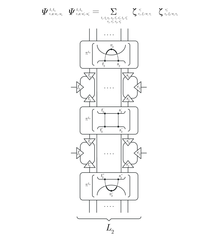
Figure 47: Right half of the graphical representation of the left side of (159).

Zooming in onto the middle part of this figure, we first insert a thick line and a summation over $t,A$ as in the first step in fig. 48.

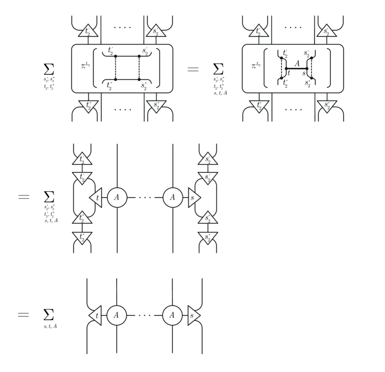
Figure 48: Manipulation of the middle part of fig. 47.

Then we write out the definition of our representation $\pi^{L_{2}}$ of $\lozenge$, corresponding to the second step in fig. 48. The summations over $t_{2},t_{2}^{\prime},s_{2},s_{2}^{\prime}$ can now be carried out yielding the final diagram in fig. 48. Inserting the identity of fig. 48 into fig. 47, we obtain fig. 49, using also the relation for $P^{L_{2}}$ in cor. 1, item 6).

Figure 49: Result of manipulations on fig. 48.

Considering the identity of fig. 49 applied to both subchains $L_{1}$ and $L_{2}$, we obtain fig. 50.

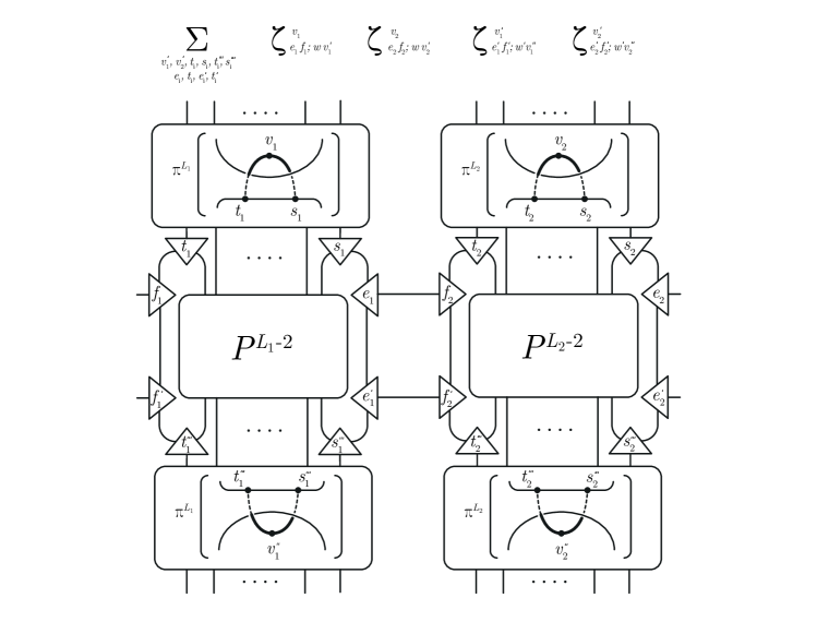
Figure 50: Result of manipulations on fig. 49.

We next focus on the middle parts of this figure involving the MPOs $P^{L_{1}-2}$ and $P^{L_{2}-2}$.

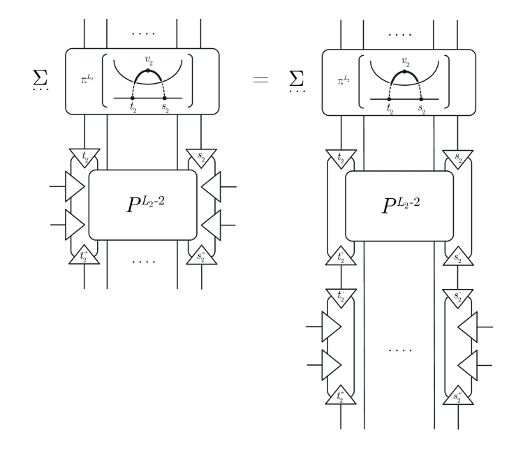
Figure 51:

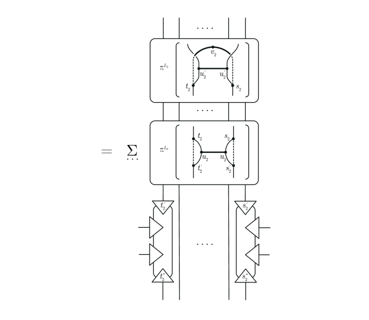
Figure 52:

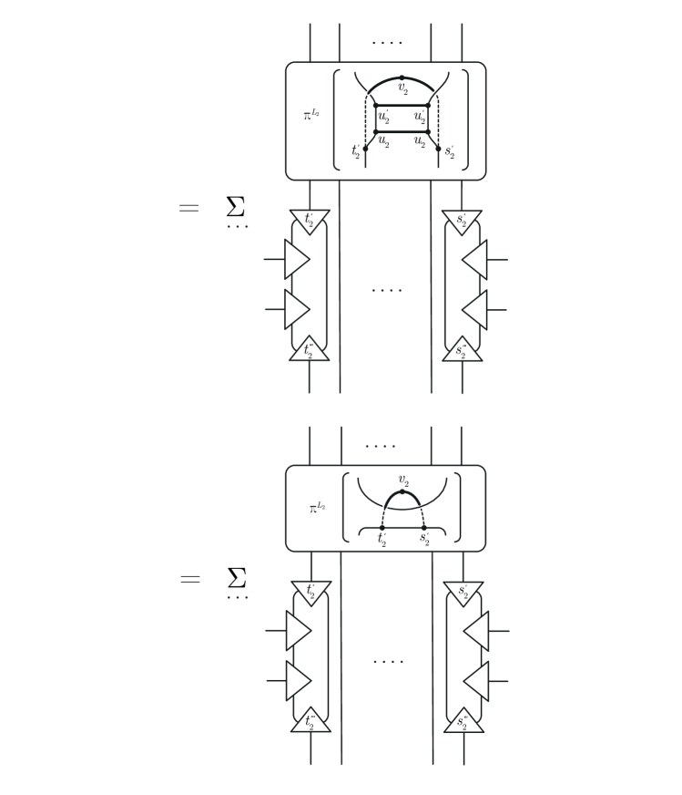
Figure 53:

In fig. 51, we first introduce summations over $t_{2},t_{2}^{\prime},s_{2},s_{2}^{\prime}$ to go to the second panel. Then we insert the expression of $P^{L_{2}-2}$ as an MPO, cor. 1, item 6), and perform simple manipulations with $6j$-symbols very similar to the proof of thm. 1 to go to fig. 52. To arrive at fig. 53, we use the representation property of $\pi^{L_{2}}$, thm. 1. To go to the second panel, we have written out the representation $\pi^{L_{2}}$ and performed simple manipulations with $6j$-symbols very similar to the proof of thm. 1. Using the representation property of $\pi^{L_{2}}$, this allows us after the steps shown in fig. 53 to eliminate the projectors $P^{L_{i}-2}$ in fig. 50 in terms of identity operators, and the figure now starts to look like structurally similar to the diagram for a single $\Psi$-operator, as in fig. 46.

With this replacement understood in fig. 46, we now zoom in onto one of the parts involving the intertwiners $e_{i},f_{i},e_{i}^{\prime},f_{i}^{\prime}$, wherein

$$e_{1}^{\prime} \in{\mathrm{Hom}}(\mu_{1}^{\prime}\nu^{\prime},\mu_{1}^{\prime\prime})$$ (175)

$$f_{1}^{\prime} \in{\mathrm{Hom}}(\rho^{\prime}\lambda_{1}^{\prime},\lambda_{1}^{\prime\prime})$$ (176)

$$e_{2}^{\prime} \in{\mathrm{Hom}}(\mu_{2}^{\prime}\rho^{\prime},\mu_{2}^{\prime\prime})$$ (177)

$$f_{2}^{\prime} \in{\mathrm{Hom}}(\nu^{\prime}\lambda_{2}^{\prime},\lambda_{2}^{\prime\prime}).$$ (178)

This is shown in figs. 54, 55.

Figure 54:

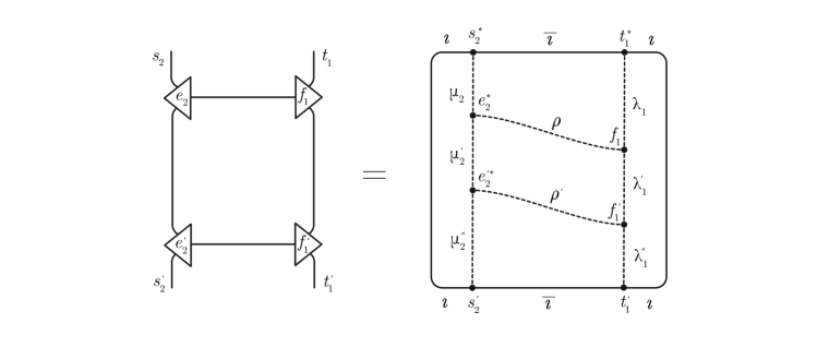
Figure 55:

The summations over ONBs of appropriate intertwiners implicit in the non-open wires yield the right panels using the properties of the $6j$-symbols. Next, we zoom in onto the $\zeta$-factors (see fig. 45) in fig. 50, which are displayed as wire-diagrams in fig. 56.

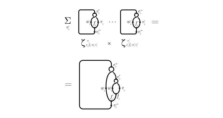
Figure 56:

We can carry out the summation over $v_{i}^{\prime}$ (for a similar argument, see the proof of thm. 1.4 in [68]), leading to the second panel. We next observe that both in fig. 54 and fig. 55, fig. 41 as well as in fig. 56, we have summations over ONBs $(1_{\rho^{\prime}}\times f_{1})f_{1}^{\prime}$, $(1_{\nu^{\prime}}\times f_{2})f_{2}^{\prime}$, $e_{1}^{\prime*}(e_{1}^{*}\times 1_{\nu^{\prime}})$, $e_{2}^{\prime*}(e_{2}^{*}\times 1_{\rho^{\prime}})$ respectively their adjoints. By unitarity of the $6j$-symbols we can switch to ONBs of the form $(f_{1}\times 1_{\lambda_{1}^{\prime}})f_{1}^{\prime}$, $(f_{2}\times 1_{\lambda_{2}^{\prime}})f_{2}^{\prime}$, $e_{1}^{\prime*}(1_{\mu_{1}^{\prime}}\times e_{1}^{*})$, $e_{2}^{\prime*}(1_{\mu_{2}^{\prime}}\times e_{2}^{*})$. The effect of this change on fig. 56 is shown in fig. 57, using also a sequence of braiding-fusion moves.

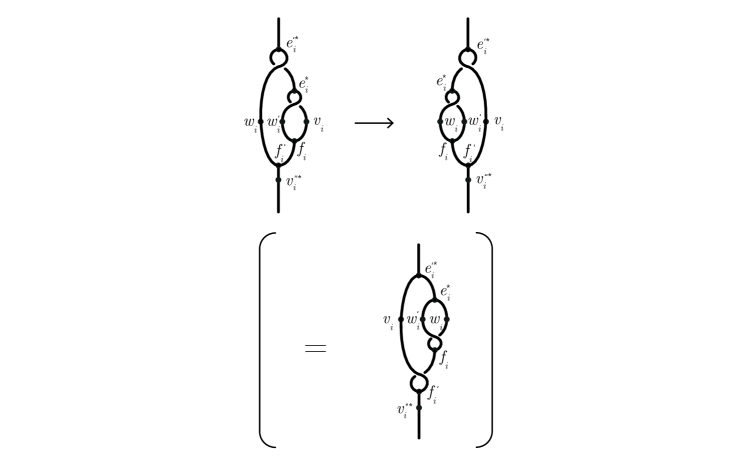
Figure 57:

Likewise, the effect of these changes on fig. 54 and fig. 55 is shown in the second panel of fig. 58 which also includes the result of fig. 57 (with a similar relation for $1\leftrightarrow 2$).

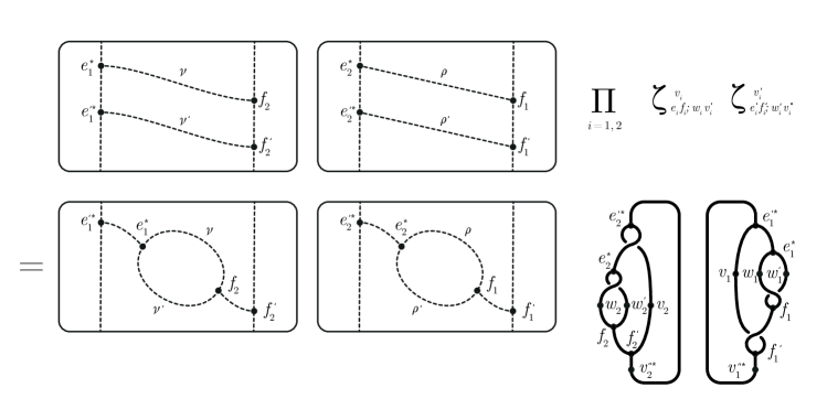
Figure 58:

In the second panel in fig. 58, we obtain from the dashed bubbles on the left side Kronecker delta’s $\delta_{e_{1},f_{2}}\delta_{e_{2},f_{1}}$. Using these delta’s and taking the rightmost wire diagrams apart via a new summation over $w_{1}^{\prime\prime},w_{2}^{\prime\prime}$ yields the second panel in fig. 59.

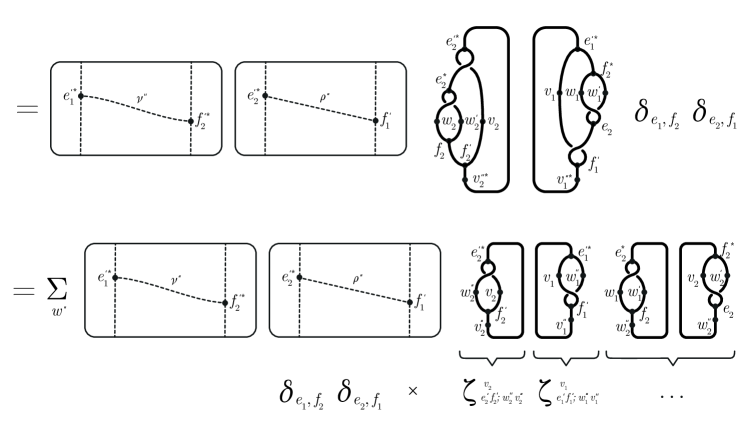
Figure 59:

We now reverse the steps fig. 54 and fig. 55 on the two leftmost square diagrams in the lower panel of fig. 59. Finally, we insert this into fig. 50, remembering that we are allowed to eliminate the projectors $P^{L_{i}-2}$ in fig. 50 in terms of identity operators. This yields the diagram for the operator sum on the right side of (159) with the structure constants

$$c^{\nu^{\prime\prime},\rho^{\prime\prime},w_{1}^{\prime\prime},w_{2}^{\prime\prime}}_{\nu^{\prime},\rho^{\prime},w_{1}^{\prime},w_{2}^{\prime};\nu,\rho;w_{1},w_{2}}:=\sum_{e,f}\zeta^{w_{1}^{\prime\prime}}_{e,f;w_{1},w_{1}^{\prime}}\zeta^{w_{2}^{\prime\prime}}_{f^{*},e^{*};w_{2},w_{2}^{\prime}}.$$ (179)

But the $\zeta$-structure constants (170) differ from the $\eta$-structure constants (102) only by a braiding operator which is unitary and hence gives a unitary change of ONB in the respective intertwiner spaces. So we can replace the $\zeta$-structure constants with the $\eta$-structure constants.

5) Consider the operator

$$(Q_{\mu_{1},\lambda_{1}}^{L_{1}}\otimes Q_{\mu_{2},\lambda_{2}}^{L_{2}})\Psi^{L_{1},L_{2}}_{\nu,\rho;w_{1},w_{2}}(Q_{\mu_{1}^{\prime},\lambda_{1}^{\prime}}^{L_{1}}\otimes Q_{\mu_{2}^{\prime},\lambda_{2}^{\prime}}^{L_{2}}).$$ (180)

We recall the representation $Q^{L}_{\mu,\nu}=\pi^{L}(q_{\mu,\nu})$ and the graphical expression for $q_{\mu,\nu}$, in the double triangle algebra, fig. 26. We insert this into fig. 47, use the representation property of $\pi^{L_{i}}$, the relations in the double triangle algebra $\lozenge$, and [58], lem. 6.2. Then we see that in the sum over intertwiners $e_{i},f_{i}$ as in (162) only such terms survive such that the values of $\mu_{i},\lambda_{i},\mu_{i}^{\prime},\lambda_{i}^{\prime}$ are equal to the values prescribed by the projections $Q$ in (180). This is equivalent to the claimed fusion property in 5). ∎

4.2 Classification of defects

According to thm. 3, 4) the defect algebra ${{\cal D}}^{L_{1},L_{2}}$ associated with a bi-partite closed spin chain with subsystems of lengths $L_{1},L_{2}$ is abelian and its structure constants are independent of $L_{1},L_{2}$. This means that the defect algebra is a representation of a universal object. In fact, it is precisely isomorphic to the algebra classifying transparent boundaries in 1+1 dimensional CFTs [5, 60], see sec. 2.10:

Theorem 4.

The defect algebra ${{\cal D}}^{L_{1},L_{2}}$ associated with a bi-partite spin chain with subsystems of lengths $L_{1},L_{2}$ is a representation of $({{\cal B}}^{+})^{\prime}\cap{{\cal B}}^{+}$, where ${{\cal B}}^{+}$ is the extension of ${{\cal N}}\otimes{{\cal N}}^{\rm opp}$ defined by the braided product Q-system $Z_{1}[X]\times^{+}Z_{2}[X]$ with $Z_{i}[X]=(\theta_{{\rm R}i},x_{{\rm R}i},w_{{\rm R}i}),i=1,2$ two copies of the full center Q-system of ${}_{{\cal N}}X_{{\cal N}}$.

Proof.

This statement is implicit in the proof of [60], prop. 4.19. First we recall the generators of $({{\cal B}}^{+})^{\prime}\cap{{\cal B}}^{+}$. By the general relation between Q-systems and extensions, ${{\cal B}}^{+}$ is pointwise equal to $NV^{+}$, with $N\in{{\cal N}}\otimes{{\cal N}}^{\rm opp}$ and with $V^{\pm}$ obeying the relations (33) for $X^{+}$ as in (40) for our two isomorphic copies of the full center Q-system. To be precise, denoting $l=(\lambda,\mu,v),\bar{l}=(\bar{\lambda},\bar{\mu},\bar{v})$ and by $T_{l}\in{{\cal N}}\otimes{{\cal N}}^{\rm opp}$ a set of isometries obeying the Cuntz algebra relations (with $\mu,\lambda\in{}_{{{\cal N}}}X_{{\cal N}},v\in{\mathrm{Hom}}(\alpha^{+}_{\lambda},\alpha_{\mu}^{-})$), we may set $\theta_{{\rm R}1}=\sum_{l}T_{l}(\lambda\otimes\mu^{\rm opp})T_{l}^{*}$ and $\theta_{{\rm R}2}=\sum_{l}T_{\bar{l}}(\bar{\lambda}\otimes\bar{\mu}^{\rm opp})T_{\bar{l}}^{*}$. By [60], lem. 4.5, the center $({{\cal B}}^{+})^{\prime}\cap{{\cal B}}^{+}$ is generated as a vector space by $P^{+}V^{+}$, where $P^{+}\in{\mathrm{Hom}}(id,\theta_{{\rm R}1}\theta_{{\rm R}2})\cap{{\cal N}}\otimes{{\cal N}}^{\rm opp}$. A basis of such $P^{+}$ is given by

$$P^{+}_{\lambda,\mu;v_{1},v_{2}}:=(\bar{r}_{\lambda}^{*}\otimes(\bar{r}_{\mu}^{\rm opp})^{*})T_{\mu,\lambda,v_{1}}^{*}\theta_{1}(T_{\bar{\mu},\bar{\lambda},\bar{v}_{2}}^{*}),$$ (181)

with $\mu,\lambda\in{}_{{{\cal N}}}X_{{\cal N}}$ and $v_{i}$ an ONB of ${\mathrm{Hom}}(\alpha^{+}_{\lambda},\alpha_{\mu}^{-})$. So, a set of generators of the center $({{\cal B}}^{+})^{\prime}\cap{{\cal B}}^{+}$ is

$$B_{\lambda,\mu,v_{1},v_{2}}=P_{\lambda,\mu;v_{1},v_{2}}V^{+}.$$ (182)

It is now straightforward to use the Q-system calculus, (33) and (40), and the definition of the full center Q-system $Z[X]$. Then it is found that

$$B_{\lambda,\mu,v_{1},v_{2}}B_{\lambda^{\prime},\mu^{\prime},v_{1}^{\prime},v_{2}^{\prime}}=\sum_{\lambda^{\prime\prime},\mu^{\prime\prime},v_{1}^{\prime\prime},v_{2}^{\prime\prime}}d^{\lambda^{\prime\prime},\mu^{\prime\prime},v_{1}^{\prime\prime},v_{2}^{\prime\prime}}_{\lambda^{\prime},\mu^{\prime},v_{1}^{\prime},v_{2}^{\prime};\lambda,\mu;v_{1},v_{2}}B_{\lambda^{\prime\prime},\mu^{\prime\prime},v_{1}^{\prime\prime},v_{2}^{\prime\prime}}$$ (183)

for the structure constants $d$ given by

$$d^{\lambda^{\prime\prime},\mu^{\prime\prime},v_{1}^{\prime\prime},v_{2}^{\prime\prime}}_{\lambda^{\prime},\mu^{\prime},v_{1}^{\prime},v_{2}^{\prime};\lambda,\mu;v_{1},v_{2}}=\sum_{e_{1},e_{2},f_{1},f_{2}}\eta^{v_{1}^{\prime\prime}}_{e_{1},f_{1};v_{1}v_{1}^{\prime}}\eta^{\bar{v}_{2}^{\prime\prime}}_{e_{2},f_{2};\bar{v}_{2}\bar{v}_{2}^{\prime}}[d(\mu^{\prime\prime})d(\lambda^{\prime\prime})]^{-1}$$ (184)

$$[(1_{\mu}\times\varepsilon^{+}(\mu^{\prime},\bar{\mu})\times 1_{\bar{\mu}^{\prime}})(f_{1}\times f_{2})r_{\mu^{\prime\prime}}]^{*}(1_{\lambda}\times\varepsilon^{-}(\lambda^{\prime},\bar{\lambda})\times 1_{\bar{\lambda}^{\prime}})(e_{1}\times e_{2})r_{\lambda^{\prime\prime}}$$

where $e_{1},e_{2},f_{1},f_{2}$ run over ONBs of ${\mathrm{Hom}}(\lambda\lambda^{\prime},\lambda^{\prime\prime}),{\mathrm{Hom}}(\bar{\lambda}\bar{\lambda}^{\prime},\bar{\lambda}^{\prime\prime}),{\mathrm{Hom}}(\mu\mu^{\prime},\mu^{\prime\prime}),{\mathrm{Hom}}(\bar{\mu}\bar{\mu}^{\prime},\bar{\mu}^{\prime\prime})$, respectively. The second line is $d(\mu^{\prime\prime})d(\lambda^{\prime\prime})$ if $e_{2}=\varepsilon^{-}(\bar{\lambda},\bar{\lambda}^{\prime})\bar{e}_{1}$ and $f_{2}=\varepsilon^{+}(\bar{\mu},\bar{\mu}^{\prime})\bar{f}_{1}$ and zero otherwise, by a set of braiding-fusion moves and by using the definition of the conjugate intertwiners. Thus, the structure constants are (writing out the $\eta$-structure constants)

$$=\sum_{e,f}\left[\frac{d(\mu)d(\mu^{\prime\prime})d(\lambda)d(\lambda^{\prime\prime})}{d(\mu^{\prime})d(\lambda^{\prime})d(\theta)^{2}}\right]^{1/2}\,E[\bar{f}^{*}\varepsilon^{-}(\bar{\mu},\bar{\mu}^{\prime})^{*}(\bar{v}_{2}\times\bar{v}_{2}^{\prime})\varepsilon^{+}(\bar{\lambda},\bar{\lambda}^{\prime})\bar{e}(\bar{v}_{2}^{\prime\prime})^{*}]E[f^{*}(v_{1}\times v_{1}^{\prime})e(v_{1}^{\prime\prime})^{*}].$$ (185)

By writing out the definition of the conjugate endomorphisms, using the functoriality condition 2) of alpha induction, and using the conjugacy relations, we arrive at,

$$E[\bar{f}^{*}\varepsilon^{-}(\bar{\mu},\bar{\mu}^{\prime})^{*}(\bar{v}_{2}\times\bar{v}_{2}^{\prime})\varepsilon^{+}(\bar{\lambda},\bar{\lambda}^{\prime})\bar{e}(\bar{v}_{2}^{\prime\prime})^{*}]=E[e^{*}((v_{2})^{*}\times(v_{2}^{\prime})^{*})fv_{2}^{\prime\prime}].$$ (186)

A comparison of (183) with (159) then shows that the map

$$B_{\lambda,\mu,v_{1},v_{2}}\mapsto\Psi^{L_{1},L_{2}}_{\lambda,\mu,v_{1},v_{2}^{*}}$$ (187)

is an algebra representation. ∎

By [5], thm. 4.44 we have a description of $({{\cal B}}^{+})^{\prime}\cap{{\cal B}}^{+}$ in terms of the objects $A\in\,_{{\cal M}}X_{{\cal M}}$; more precisely for each $A$ one can construct in a canonical way a minimal projection $p_{A}\in({{\cal B}}^{+})^{\prime}\cap{{\cal B}}^{+}$. The element $D_{A}^{L_{1},L_{2}}\in{{\cal D}}^{L_{1},L_{2}}$ corresponding to $p_{A}$ under the above representation (187) is a projection operator acting on $\mathscr{V}^{L_{1}}_{\rm open}\otimes\mathscr{V}^{L_{2}}_{\rm open}$ which by definition must be of the form

$$D_{A}^{L_{1},L_{2}}=\sum_{\nu,\rho,w_{1},w_{2}}\xi_{A;\nu,\rho,w_{1},w_{2}}\Psi_{\nu,\rho;w_{1},w_{2}}^{L_{1},L_{2}}$$ (188)

for certain complex numbers $\xi_{A;\nu,\rho,w_{1},w_{2}}$. These complex numbers are in principle determined by [5], thm. 4.44 and are universal, i.e. independent of $L_{1},L_{2}$ or the dynamics on the spin-chain. In general, it seems nontrivial to determine them from data that are directly accessible, so we will leave this problem to a future work. If we have the projections $D_{A}^{L_{1},L_{2}}$, we can write

$$\mathscr{V}^{L_{1}}_{\rm open}\otimes\mathscr{V}^{L_{2}}_{\rm open}=\bigoplus_{A\in\,_{{\cal M}}X_{{\cal M}}}\mathscr{V}^{L_{1},L_{2}}_{A},\quad\mathscr{V}^{L_{1},L_{2}}_{A}:=D_{A}^{L_{1},L_{2}}(\mathscr{V}^{L_{1}}_{\rm open}\otimes\mathscr{V}^{L_{2}}_{\rm open}).$$ (189)

The subspaces $\mathscr{V}^{L_{1},L_{2}}_{A}$ determine a specific boundary condition $A$ fusing the two chains $L_{1},L_{2}$ together. By thm. 3, 3) these subspaces are invariant under the action of any local operator which does not act on the endpoint of the two chains.

4.3 Special cases: abelian fusion in ${{\cal M}}$

There is an interesting special case, still covering many examples, where the determination of the coefficients $\xi_{A;\nu,\rho,w_{1},w_{2}}$ in (188) is possible, namely when all $Z_{\nu,\rho}\in\{0,1\}$. Then, since the horizontal center ${{\cal Z}}_{h}$ is isomorphic to the fusion ring $\,{}_{{\cal M}}X_{{\cal M}}$, and since the direct summands of ${{\cal Z}}_{h}$ are matrix algebras of size $Z_{\nu,\rho}$, it follows that $\,{}_{{\cal M}}X_{{\cal M}}$ is abelian, i.e. $N_{A,B}^{C}=N_{B,A}^{C}$ in particular ($\,{}_{{\cal N}}X_{{\cal N}}$ by assumption is always abelian because we assume that it is braided). In such a situation, the pairs $(\nu,\rho)$ such that $Z_{\nu,\rho}=1$ are one-to-one correspondence with the simple objects $A\in\,_{{\cal M}}X_{{\cal M}}$. In fact, since we have $Z_{\nu,\rho}=\sum_{B}\langle\alpha^{+}_{\nu},B\rangle\langle\alpha^{-}_{\rho},B\rangle$, with $\langle\alpha^{\pm}_{\lambda},B\rangle={\mathrm{dim}}{\mathrm{Hom}}(\alpha^{\pm}_{\lambda},B)$, we may assign to $(\nu,\rho)$ that unique $B$ corresponding to the only summand which is $=1$.

In particular, we may diagonalize the fusion coefficients $N_{A,B}^{C}$. Furthermore, since $Z_{\nu,\rho}={\mathrm{dim}}{\mathrm{Hom}}(\alpha^{-}_{\rho},\alpha^{+}_{\nu})\in\{0,1\}$, we have no need for the degeneracy indices $w_{1},w_{2}$ so that we may write write $\Psi_{\nu,\rho}^{L_{1},L_{2}}$ for the MPOs generating the defect algebra. By [60], sec. 5.4, the coefficients (188) are proportional to the inverse of the matrices diagonalizing $N_{A,B}^{C}$. By lem. 2, 1) and 3), the latter are in turn given by the coefficients $Y_{\lambda,\mu,A}$ given in fig. 27 . Combining these results gives

$$D_{A}^{L_{1},L_{2}}=\frac{d_{A}}{D_{X}^{2}d^{4}}\sum_{\nu,\rho}d_{\nu}d_{\rho}\,Y_{\nu,\rho,A}\Psi_{\nu,\rho}^{L_{1},L_{2}}.$$ (190)

At any rate, this makes the determination of the $D_{A}^{L_{1},L_{2}}$ a feasible problem, because $N_{A,B}^{C}$ is known from the start.

In the case of a diagonal fusion category ${}_{{\cal N}}X_{{\cal N}}$,

$$Z_{\nu,\rho}=\delta_{\nu,\rho},$$ (191)

we have $|{}_{{\cal N}}X_{{\cal N}}|=|{}_{{\cal M}}X_{{\cal M}}|$ and $\delta_{\nu,\rho}=\sum_{B}\langle\alpha^{+}_{\nu},B\rangle\langle\alpha^{-}_{\rho},B\rangle$ meaning that $(\langle\alpha^{\pm}_{\lambda},A\rangle)_{\lambda\in{}_{{\cal N}}X_{{\cal N}},A\in{}_{{\cal M}}X_{{\cal M}}}$ are permutation matrices which are inverses of each other, setting up a bijection between the simple objects in ${}_{{\cal N}}X_{{\cal N}}$ and ${}_{{\cal M}}X_{{\cal M}}$. Due to the homomorphism property of $\alpha$-induction, either one of these isomorphisms transforms the $N_{\mu,\nu}^{\sigma}$ fusion coefficients to the $N_{A,B}^{C}$ fusion coefficients.

The defect operators $\Psi_{\nu,\nu}^{L_{1},L_{2}}$ may be labelled by $A\in{}_{{\cal M}}X_{{\cal M}}$ under this isomorphism, so we may write $\Psi_{A}^{L_{1},L_{2}}$. As a special case of (159), their OPE is (after a suitable renormalization of the generators)

$$\Psi_{A}^{L_{1},L_{2}}\Psi_{B}^{L_{1},L_{2}}=\sum_{C}N_{A,B}^{C}\Psi_{C}^{L_{1},L_{2}},$$ (192)

so is an isomorphic copy of the abelian fusion product in ${}_{{\cal M}}X_{{\cal M}}$. Thus, in this special case, the defect algebra ${{\cal D}}^{L_{1},L_{2}}$ is an isomorphic copy of this fusion ring. By contrast to the MPOs $O_{A}^{L}$, which also yield an algebra isomorphic to the fusion ring of ${}_{{\cal M}}X_{{\cal M}}$ by (110), thm. 1, the MPOs $\Psi_{A}^{L_{1},L_{2}}$ act on a bipartite chain. Therefore, by contrast to the former, we think of them as corresponding to vertical, instead of horizontal, defects.

Note that for non-diagonal theories, the fusion ring of ${}_{{\cal M}}X_{{\cal M}}$ can be non-abelian, while ${{\cal D}}^{L_{1},L_{2}}$ is always abelian. Thus, in general, the horizontal defect algebra (the $O_{A}^{L}$s) is not isomorphic to our vertical defect algebra (the $\Psi_{\nu,\rho;w_{1},w_{2}}^{L_{1},L_{2}}$).

5 Conclusions

In this paper we have explored some connections between subfactor theory, braided unitary fusion categories, CFTs in $1+1$ dimensions, defects, and anyonic spin chains. Future work should address the following points:

• We have not addressed at all the analytic question of scaling limits of anyonic spin chains. To what extent will the close analogy between the defect algebra in on the spin-chain and of the CFTs – observed here at a purely algebraic level for finite chains – persist in such a scaling limit?

• Our defect operators on the spin-chains have, after all, a fairly complicated structure. What simplifications can be obtained in simple cases such as the anyonic chain built upon the Ising fusion category?

• If one already knows that the fusion categories used as an input into the anyonic chain construction came from a CFT, such as e.g. arising from the positive energy highest weight representations of a Virasoro algebra in the case the minimal models: Can the vacuum state of the CFT be used to obtain an approximation of the ground state for the anyonic chain?

Acknowledgements: I thank Henning Rehren and Yasu Kawahigashi for their educational emails related to subfactors and CFTs, and Laurens Lootens, Alex Stottmeister and Frank Verstraete for explanations regarding anyonic spin chains. I am grateful to the Max-Planck Society for supporting the collaboration between MPI-MiS and Leipzig U., grant Proj. Bez. M.FE.A.MATN0003, and to Thomas Endler from MPI-MiS, Leipzig, for help with figures.

Appendix A Inclusions associated with finite groups

Let ${{\cal N}}\subset{{\cal M}}$ be an irreducible inclusion of factors such that $\gamma({{\cal M}})^{\prime}\cap{{\cal M}}={{\cal N}}_{1}^{\prime}\cap{{\cal M}}$ is abelian with dimension $n=[{{\cal M}}:{{\cal N}}]$. [72] has shown that ${{\cal N}}={{\cal M}}^{\alpha}$, where $g\mapsto\alpha_{g}$ is an action of a finite group $G$ of order $n$ by outer automorphisms acting on ${{\cal M}}$. This situation is in principle very well-understood, see e.g. [67] who uses the Cuntz-algebra picture. Here we work out the situation totally explicitily from the Q-system perspective as an illustration of this concept for the reader without a background in subfactor theory.

A. By the general theory since ${{\cal M}}={{\cal N}}v$ point-wise there must exist a unique $u_{g}\in{{\cal N}}$ such that

$$\alpha_{g}(v)=u_{g}v,\quad u_{g}\in{{\cal N}}.$$ (193)

Using $\alpha_{g}\alpha_{h}(v)=\alpha_{gh}(v)$ and $\alpha_{g}(v)^{*}=\alpha_{g}(v^{*})$ or $\alpha_{g}(v^{2})=[\alpha_{g}(v)]^{2}$ respectively, we find

$$\quad u_{g}u_{h}=u_{gh},\quad u_{g}^{*}r=\theta(u_{g})r,\quad xu_{g}\theta(u_{g})=u_{g}x,$$ (194)

with $r=xw\in{\mathrm{Hom}}(\theta^{2},id)$. Using $\alpha_{g}(n)=n,n\in{{\cal N}}$, we also find $[u_{g},\theta({{\cal N}})]=0$ so $u_{g}\in{\mathrm{Hom}}(\theta,\theta)\cap{{\cal N}}$. Also, $\theta=j_{{\cal N}}j_{{\cal M}}|_{{{\cal N}}}=j_{{{\cal N}}_{1}}j_{{\cal N}}|_{{{\cal N}}}$, so $\theta({{\cal N}})={{\cal N}}_{2}$ and hence $u_{g}\in{{\cal N}}_{2}^{\prime}\cap{{\cal N}}$.

B. We can rewrite the decomposition $\theta\cong\oplus_{i}{\rho}_{i}$ where a given sector may appear multiple times, as $\theta\cong\oplus_{\pi}d_{\pi}\cdot{\rho}_{\pi}$, where $d_{\pi}$ is the multiplicity of the irreducible sector ${\rho}_{\pi}$. The corresponding intertwiners are $w^{a}_{\pi},a=1,\dots,d_{\pi}$, and

$$\theta(n)=\sum_{\pi}\sum_{a=1}^{d_{\pi}}w^{a}_{\pi}{\overline{\rho}}_{\pi}(n)w^{a*}_{\pi}.$$ (195)

It follows from the intertwiner calculus that

$$D_{\pi}(g)_{a}^{b}=w^{a*}_{\pi}u_{g}w^{b}_{\pi}\in{{\cal N}}\cap{\mathrm{Hom}}(\bar{\rho}_{\pi},\bar{\rho}_{\pi})=\mathbb{C}1,$$ (196)

can be identified with complex numbers, and the $d_{\pi}\times d_{\pi}$ matrices $D_{\pi}(g)_{a}^{b}$ form an irreducible representation of $G$ which transforms the fields $\psi^{a}_{\pi}:=w_{\pi}^{a*}v$ as in

$$\alpha_{g}(\psi^{b}_{\pi})=\sum_{a=1}^{d_{\pi}}D_{\pi}(g)_{a}^{b}\psi^{a}_{\pi}.$$ (197)

One can equip the linear space $\mathscr{K}_{\pi}={\rm span}_{\mathbb{C}}\{\psi^{a}_{\pi}:a=1,\dots,d_{\pi}\}$ with a scalar product $(\phi_{1},\phi_{2})_{\pi}1=\phi_{1}^{*}\phi_{2}$ because the latter operator is an intertwiner in ${\mathrm{Hom}}(id,id)$ which is at the same time in ${{\cal M}}$ hence in ${{\cal N}}^{\prime}\cap{{\cal M}}=\mathbb{C}1$. Then it follows that the numerical matrices $D_{\pi}(g)_{a}^{b}$ give a unitary operator $D_{\pi}(g)$ on $\mathscr{K}_{\pi}$ which implements $\alpha_{g}(\phi)=D_{\pi}(g)\phi$ (unitarity because $\phi_{1}^{*}\phi_{2}=\alpha_{g}(\phi_{1})^{*}\alpha_{g}(\phi_{2})$ from $\alpha_{g}(1)=1$.) Thus, $u_{g}$ itself

$$u_{g}=\sum_{\pi}\sum_{a,b=1}^{d_{\pi}}D_{\pi}(g)_{a}^{b}w^{a}_{\pi}w^{b*}_{\pi}$$ (198)

is unitary. Thus $\pi$ corresponds to the unitary irreducible representations of $G$, with characters

$$\chi_{\pi}(g)=\sum_{a=1}^{d_{\pi}}D_{\pi}(g)_{a}^{a}.$$ (199)

C. Now let

$$u_{g}^{\prime}=j_{{\cal N}}(u_{g})\in{{\cal N}}^{\prime}.$$ (200)

The unitaries $u_{g}^{\prime}\in{{\cal N}}^{\prime}$ also form a representation of $G$. For the minimal expectation $E^{\prime}:{{\cal N}}^{\prime}\to{{\cal M}}^{\prime}$ we calculate

$$E^{\prime}(u_{g}^{\prime})=\frac{1}{d}w^{\prime*}\gamma^{\prime}(u_{g}^{\prime})w^{\prime}=\frac{1}{d}j_{{\cal M}}(v^{*}u_{g}v)$$ (201)

using $w^{\prime}=j_{{\cal M}}(v)$. Since $u_{g}\in{\mathrm{Hom}}(\theta,\theta),v\in{\mathrm{Hom}}(\theta,id)$, we must have $v^{*}u_{g}v\in{{\cal N}}^{\prime}\cap{{\cal M}}=\mathbb{C}1$. To compute this number, we apply again $E$, since $E(v^{*}u_{g}v)=v^{*}u_{g}v$,

$$\begin{split}E(v^{*}u_{g}v)=&\sum_{\pi}\sum_{a,b=1}^{d_{\pi}}D_{\pi}(g)_{a}^{b}E(v^{*}w^{a}_{\pi}w^{b*}_{\pi}v)\\ =&\sum_{\pi}\sum_{a,b=1}^{d_{\pi}}D_{\pi}(g)_{a}^{b}\frac{{\mathrm{dim}}({\bar{\rho}}_{\pi})}{d}\delta^{a}_{b}\\ =&\sum_{\pi}\chi_{\pi}(g)\frac{d_{\pi}}{d}=d\cdot\delta_{1,g}.\end{split}$$ (202)

Thus, $E^{\prime}(u_{g}^{\prime})=\delta_{1,g}$.

D. Let $e\equiv e_{{{\cal M}}^{\prime}}=[{{\cal M}}^{\prime}\eta]=d^{-1}\cdot vv^{*}\in{{\cal M}}\cap{{\cal N}}_{1}^{\prime}$ be the Jones projection for the extension ${{\cal N}}_{1}\subset{{\cal N}}$. (Since $j_{{\cal N}}(e_{{{\cal N}}_{1}})=e_{{{\cal N}}_{1}}$ and $j_{{\cal N}}({{\cal N}}_{1})={{\cal M}}^{\prime}$ we have $e_{{{\cal N}}_{1}}=e_{{{\cal M}}^{\prime}}$.) Then $E(e)=d^{-2}1$. On the other hand

$$\begin{split}1=&d^{2}\cdot E(e)=d^{2}\cdot j_{{\cal N}}(E(e))=d\cdot j_{{\cal N}}(E(vv^{*}))\\ =&\frac{d}{|G|}j_{{\cal N}}\left(\sum_{g}\alpha_{g}(vv^{*})\right)\\ =&\frac{d}{|G|}\sum_{g}j_{{\cal N}}(u_{g}vv^{*}u_{g}^{*})\\ =&\frac{d^{2}}{|G|}\sum_{g}u_{g}^{\prime}j_{{{\cal N}}}(e)u_{g}^{\prime*}\\ =&\sum_{g}u_{g}^{\prime}eu_{g}^{\prime*}\end{split}$$ (203)

since $|G|=d^{2}$ On the other hand, for any $n^{\prime}\in{{\cal N}}$,

$$n^{\prime}e=1n^{\prime}e=\sum_{g}u_{g}^{\prime}eu_{g}^{\prime*}n^{\prime}e=\sum_{g}u_{g}^{\prime}E^{\prime}(u_{g}^{\prime*}n^{\prime})e$$ (204)

in view of $E^{\prime}(n^{\prime})e=en^{\prime}e$, and so

$$n^{\prime}=\sum_{g}u_{g}^{\prime}m_{g}^{\prime},\quad m^{\prime}_{g}=E^{\prime}(u_{g}^{\prime*}n^{\prime})\in{{\cal M}}^{\prime}.$$ (205)

By $E^{\prime}(u_{g}^{\prime})=\delta_{1,g}$ this representation $n^{\prime}=\sum_{g}u_{g}^{\prime}m_{g}^{\prime}$ is unique.

E. By construction $\alpha_{g}(e)\in{{\cal M}}$ and since $\alpha_{g}({{\cal N}}_{1})={{\cal N}}_{1}$ pointwise, also $\alpha_{g}(e)\in{{\cal N}}_{1}^{\prime}$. Now $j_{{\cal N}}$ fixes ${{\cal M}}\cap{{\cal N}}_{1}^{\prime}$, so $j_{{\cal N}}(\alpha_{g}(e))\in{{\cal M}}\cap{{\cal N}}_{1}$. Since $e=d^{-1}\cdot vv^{*}$ and since we have $\alpha_{g}(v)=u_{g}v,u_{g}^{\prime}=j_{{\cal N}}(u_{g})$, and $j_{{\cal N}}(e)=e$, we have $u_{g}^{\prime}eu_{g}^{\prime*}\equiv e_{g}\in{{\cal M}}\cap{{\cal N}}_{1}^{\prime}$. By the Jones basic construction, ${{\cal N}}_{1}^{\prime}={{\cal N}}^{\prime}\vee\{e\},{{\cal M}}={{\cal N}}\vee\{e\}$, so in particular $u_{g}^{\prime}{{\cal M}}u_{g}^{\prime*}={{\cal M}}$ and hence also $u_{g}^{\prime}{{\cal M}}^{\prime}u_{g}^{\prime*}={{\cal M}}^{\prime}$. In conclusion, we have ${{\cal N}}^{\prime}={{\cal M}}^{\prime}\vee\{u^{\prime}_{g}\}$, and the properties of the $u_{g}^{\prime}$ and of $E^{\prime}$ in D show that this is crossed product of ${{\cal M}}^{\prime}$ by an action of $G$. We may thus say that

$${{\cal N}}={{\cal M}}^{\alpha},\quad{{\cal N}}^{\prime}={{\cal M}}^{\prime}\rtimes_{\alpha^{\prime}}G,$$ (206)

where $\alpha^{\prime}_{g}(m^{\prime})=u_{g}^{\prime}m^{\prime}u_{g}^{\prime*}$ is an action of $G$ on ${{\cal M}}^{\prime}$.

F. By (203) and E, $1=\sum_{g}e_{g}$. Recall that ${{\cal M}}\cap{{\cal N}}_{1}^{\prime}$ is abelian of dimension $|G|$. Thus, the $e_{g}$ are commuting projections. They are either pairwise distinct or $e_{g}=e$ for all $g$ which is not possible so the $e_{g}$ are the minimal projections for ${{\cal M}}\cap{{\cal N}}_{1}^{\prime}$.

G. $\alpha^{\prime}$ is also an action on ${{\cal M}}$, and by $u_{g}^{\prime}\in{{\cal N}}^{\prime}$, we have ${{\cal N}}\subset{{\cal M}}^{\alpha^{\prime}}\subset{{\cal M}}$. However since ${{\cal N}}^{\prime}\cap{{\cal M}}$, this action is outer and hence $[{{\cal N}}:{{\cal M}}]=|G|=[{{\cal M}}^{\alpha^{\prime}}:{{\cal M}}]$, thus ${{\cal M}}^{\alpha^{\prime}}={{\cal N}}$. Then, we may repeat the same procedures A–F with potentially new $\tilde{u}_{g}^{\prime}\in{{\cal N}}^{\prime}$. By D, F $\tilde{u}_{g}^{\prime}e\tilde{u}_{g}^{\prime*}=e_{g}$ and thus $u_{g}^{\prime*}\tilde{u}_{g}^{\prime}\equiv w_{g}^{\prime}\in\{e\}^{\prime}$ so $w_{g}^{\prime}\in{{\cal M}}^{\prime}$. Thus, the above statements remain true with obvious modifications if we replace $\alpha$ by $\alpha^{\prime}$

We can summarize the situation as follows:

Proposition 1.

Let ${{\cal N}}\subset{{\cal M}}$ be an irreducible inclusion of factors such that $\gamma({{\cal M}})^{\prime}\cap{{\cal M}}$ is abelian with dimension $n=[{{\cal M}}:{{\cal N}}_{1}]$. Then there exist a finite group $G$ of order $n$ and $\{u_{g}^{\prime}:g\in G\}\subset{{\cal N}}^{\prime}$ such that

1. $g\mapsto u_{g}^{\prime}$ is a unitary representation of $G$.

2. ${{\cal N}}^{\prime}={{\cal M}}^{\prime}\vee\{u_{g}^{\prime}:g\in G\}$ and each $n^{\prime}\in{{\cal N}}^{\prime}$ is representable uniquely as $n^{\prime}=\sum_{g}u_{g}^{\prime}m_{g}^{\prime}$ with $m_{g}^{\prime}\in{{\cal M}}^{\prime}$.

3. $m\mapsto u_{g}^{\prime}mu_{g}^{\prime*}$ is an outer action of $G$ transforming ${{\cal M}}$ to itself. Its fixed points are exactly the elements from ${{\cal N}}$.

4. ${{\cal M}}={{\cal N}}\vee\{\psi^{a}_{\pi}:\pi\in\hat{G},a=1,\dots,d_{\pi}\}$ and each $m\in{{\cal M}}$ is uniquely representable as $m=\sum_{\pi,a}n^{a}_{\pi}\psi^{a}_{\pi}$ with $n^{a}_{\pi}\in{{\cal N}}$. $\psi^{a}_{\pi}$ are scaled isometries with $(\psi_{\pi}^{a})^{*}\psi^{a}_{\pi}=(d_{\pi}/d)1$.

5. For any $g\in G$:

   $$u^{\prime}_{g}\psi^{b}_{\pi}u_{g}^{\prime*}=\sum_{a=1}^{d_{\pi}}D_{\pi}(g)_{a}^{b}\psi^{a}_{\pi}.$$ (207)

   where $D_{\pi}$ is an irreducible representation of dimension $d_{\pi}$.

6. The canonical expectations $E:{{\cal M}}\to{{\cal N}},E^{\prime}:{{\cal N}}^{\prime}\to{{\cal M}}^{\prime}$ are given respectively by $E^{\prime}(u^{\prime}_{g})=\delta_{1,g}1,E(\psi^{a}_{\pi})=\sqrt{d}\ \delta_{\pi,0}1$.

Appendix B PEPs and double triangle algebra

We represent an MPO $O_{A}^{L}$ as an elementary cell as in fig. 31 for some fixed chosen, e.g. $L=8$. Considering a number of such a elementary building block, we build a network as indicated in fig. 60 by concatenating the outer legs of each cell, where for our choice $L=8$ we have an octagonal lattice.Such a network can be considered as a tensor with a very large number of indices given by the labels carried by the uncontracted inner lines of each cell. For each elementary cell, we have an index $A\in{}_{{\cal M}}X_{{\cal M}}$. Each index $A$ associated with a cell is now summed, weighted by the coefficient $d_{A}$, thereby effectively inserting a projector $P^{L}=Q_{id,id}^{L}$ as in fig. 61 into each cell. Such a structure, proposed in [29] is called a “PEPS” (projected entangled pair-) state. In principle, we could have taken the pair $(\mu,\nu)$ to be different for each cell, but we will see from the next “pull-through” lemma that in such a case the PEPS is zero.

Figure 60: Schematic diagram for the PEPS.

Figure 61: Schematic diagram for the insertion of the MPO $P^{L}$ into a cell. Here $L=8$.

We can also insert a string corresponding to a representer of the double triangle algebra such as $O_{A}$ into the PEPS as shown in fig. 62. The precise location of the string is irrelevant, again by the “pull-through” property of [29]:

Proposition 2.

We have the pull-through identity in fig. 62.

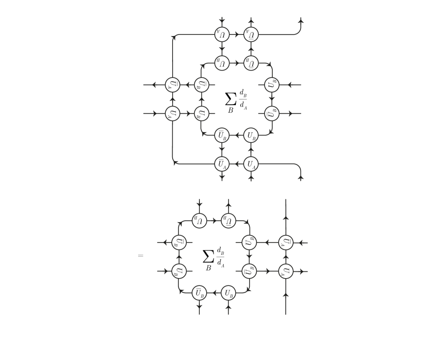
Figure 62: The pull-through property described in [29].

Proof.

A graphical proof is given by [29], but it is not so clear to us how their assumptions precisely correspond to our setting. So we argue instead as follows. First, the zipper lemma implies that the pull through property is equivalent to the equality shown graphically in fig. 63.

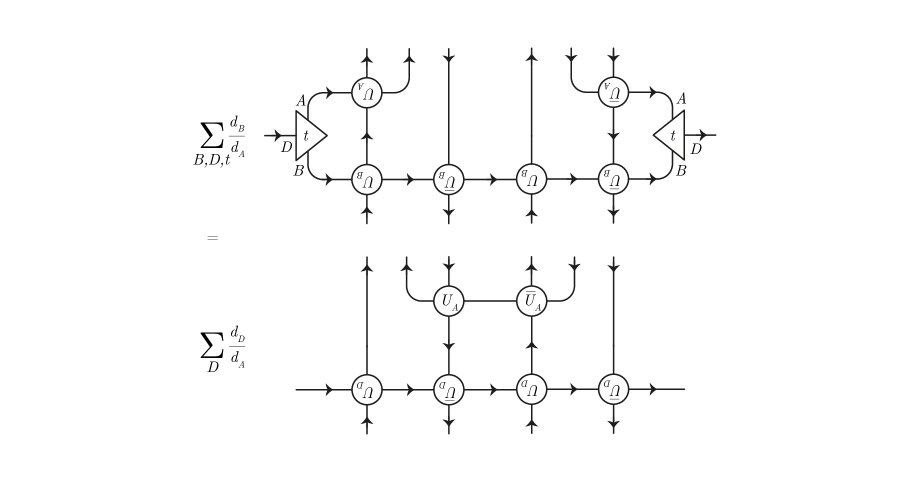
Figure 63: Equivalent form of the pull through property.

Here and in the following, we put arrows on the cells to see more clearly that the tensor contractions implied by the connected lines are well-defined, i.e. over indices in the correct intertwiner spaces. Then we contract suitable legs with $U_{B}$ and use the duality and unitarity of the $6j$-symbols as in lemma 1. This turns the desired equality into fig. 64.

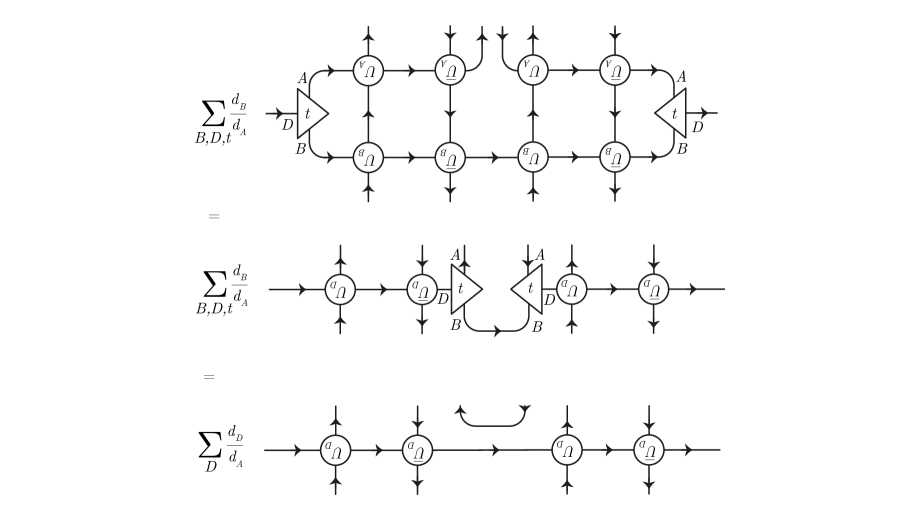
Figure 64: Upper panel: Equivalent form of the upper panel in fig. 63 after contracting into suitable legs of a $6j$-symbol. Middle panel: Obtained from upper panel by zipper lemma. Lower panel: Equivalent form of the lower panel in fig. 63 after contracting into suitable legs of a $6j$ symbol, using duality and unitarity.

Thus, we need to show the equality between the middle and lower panel in fig. 64. This equality holds true by an orthogonality property of the zipper tensors, with ONBs

$$\begin{split}&t_{8}\in{\mathrm{Hom}}_{{\cal M}}(a_{3},Ca_{1},),\\ &t_{8}^{\prime}\in{\mathrm{Hom}}_{{\cal M}}(a_{3}^{\prime},Ca_{1}),\\ &t_{3}\in{\mathrm{Hom}}_{{\cal M}}(a_{2},Ba_{1}),\\ &t_{5}^{\prime}\in{\mathrm{Hom}}_{{\cal M}}(a_{2},Aa_{1}),\\ &t_{5}\in{\mathrm{Hom}}_{{\cal M}}(a_{2},Aa_{1}),\\ &t_{0}\in{\mathrm{Hom}}_{{\cal M}}(C,AB),\end{split}$$ (208)

and $a_{i},a_{i}^{\prime}\in{}_{{\cal M}}X_{{\cal N}}$, $A,B,C\in{}_{{\cal M}}X_{{\cal M}}$:

$$\sum_{B}\sum_{t_{3},t_{0}}\frac{d_{A}}{d_{C}}\overline{\overline{Y}_{A,B}^{C}\begin{pmatrix}&t_{3}&\\ t_{0};&&t_{8}\\ &t_{5}&\end{pmatrix}}\overline{Y}_{A,B}^{C}\begin{pmatrix}&t_{3}&\\ t_{0};&&t_{8}^{\prime}\\ &t_{5}^{\prime}&\end{pmatrix}=\delta_{t_{5},t_{5}^{\prime}}\delta_{t_{8},t_{8}^{\prime}}\delta_{a_{3},a_{3}^{\prime}},$$ (209)

which follows from repeated application of Frobenius duality. This implies the statement. ∎

Instead of inserting $P^{L}$ into each cell, we could also think of inserting $Q_{\mu,\nu}^{L}$, which also is a projection (cor. 1). Thus, in a sense, we would get a different “sector” for every choice of $Q_{\mu,\nu}^{L}$, and furthermore, the standard choice $P^{L}$ proposed by [29] and investigated further by [39, 40] is included by putting $\mu=\nu=id$. We think that it is worthwhile investigating such constructions further.

References

- [1] F. Wilczek, “Quantum mechanics of fractional-spin particles,” Physical review letters, vol. 49, no. 14, p. 957, 1982.
- [2] E. Rowell, R. Stong, and Z. Wang, “On classification of modular tensor categories,” Communications in Mathematical Physics, vol. 292, no. 2, pp. 343–389, 2009.
- [3] B. Bakalov and A. A. Kirillov, Lectures on tensor categories and modular functors, vol. 21. American Mathematical Soc., 2001.
- [4] J. Fröhlich, J. Fuchs, I. Runkel, and C. Schweigert, “Correspondences of ribbon categories,” Advances in Mathematics, vol. 199, no. 1, pp. 192–329, 2006.
- [5] M. Bischoff, Y. Kawahigashi, R. Longo, and K.-H. Rehren, Tensor categories and endomorphisms of von Neumann algebras: With applications to quantum field theory, vol. 3. Springer, 2015.
- [6] P. Etingof, D. Nikshych, and V. Ostrik, “On fusion categories,” Annals of Mathematics, pp. 581–642, 2005.
- [7] G. Moore and N. Seiberg, “Classical and quantum conformal field theory,” Communications in Mathematical Physics, vol. 123, no. 2, pp. 177–254, 1989.
- [8] G. Moore and N. Seiberg, “Lectures on rcft,” in Physics, geometry and topology, pp. 263–361, Springer, 1990.
- [9] K. Fredenhagen, K.-H. Rehren, and B. Schroer, “Superselection sectors with braid group statistics and exchange algebras,” Communications in Mathematical Physics, vol. 125, no. 2, pp. 201–226, 1989.
- [10] K. Fredenhagen, K.-H. Rehren, and B. Schroer, “Superselection sectors with braid group statistics and exchange algebras ii: Geometric aspects and conformal covariance,” Reviews in Mathematical Physics, vol. 4, no. spec01, pp. 113–157, 1992.
- [11] E. Witten, “Quantum field theory and the jones polynomial,” Communications in Mathematical Physics, vol. 121, no. 3, pp. 351–399, 1989.
- [12] J. Fuchs, I. Runkel, and C. Schweigert, “Tft construction of rcft correlators i: Partition functions,” Nuclear Physics B, vol. 646, no. 3, pp. 353–497, 2002.
- [13] J. Fuchs, I. Runkel, and C. Schweigert, “Tft construction of rcft correlators: Iii: Simple currents,” Nuclear Physics B, vol. 694, no. 3, pp. 277–353, 2004.
- [14] J. Fuchs, I. Runkel, and C. Schweigert, “Tft construction of rcft correlators iv:: Structure constants and correlation functions,” Nuclear physics B, vol. 715, no. 3, pp. 539–638, 2005.
- [15] R. Longo, “Index of subfactors and statistics of quantum fields. i,” Communications in mathematical physics, vol. 126, no. 2, pp. 217–247, 1989.
- [16] R. Longo, “Index of subfactors and statistics of quantum fields,” Communications in mathematical physics, vol. 130, no. 2, pp. 285–309, 1990.
- [17] Z. Wang, Topological quantum computation. No. 112, American Mathematical Soc., 2010.
- [18] A. Kitaev, “Anyons in an exactly solved model and beyond,” Annals of Physics, vol. 321, no. 1, pp. 2–111, 2006.
- [19] A. Feiguin, S. Trebst, A. W. Ludwig, M. Troyer, A. Kitaev, Z. Wang, and M. H. Freedman, “Interacting anyons in topological quantum liquids: The golden chain,” Physical review letters, vol. 98, no. 16, p. 160409, 2007.
- [20] S. Trebst, M. Troyer, Z. Wang, and A. W. Ludwig, “A short introduction to fibonacci anyon models,” Progress of Theoretical Physics Supplement, vol. 176, pp. 384–407, 2008.
- [21] C. Gils, E. Ardonne, S. Trebst, A. W. Ludwig, M. Troyer, and Z. Wang, “Collective states of interacting anyons, edge states, and the nucleation of topological liquids,” Physical review letters, vol. 103, no. 7, p. 070401, 2009.
- [22] C. Gils, E. Ardonne, S. Trebst, D. A. Huse, A. W. Ludwig, M. Troyer, and Z. Wang, “Anyonic quantum spin chains: Spin-1 generalizations and topological stability,” Physical Review B, vol. 87, no. 23, p. 235120, 2013.
- [23] S. Trebst, E. Ardonne, A. Feiguin, D. A. Huse, A. W. Ludwig, and M. Troyer, “Collective states of interacting fibonacci anyons,” Physical review letters, vol. 101, no. 5, p. 050401, 2008.
- [24] E. Ardonne, J. Gukelberger, A. W. Ludwig, S. Trebst, and M. Troyer, “Microscopic models of interacting yang–lee anyons,” New Journal of Physics, vol. 13, no. 4, p. 045006, 2011.
- [25] R. Vanhove, L. Lootens, M. Van Damme, R. Wolf, T. Osborne, J. Haegeman, and F. Verstraete, “A critical lattice model for a haagerup conformal field theory,” arXiv preprint arXiv:2110.03532, 2021.
- [26] T.-C. Huang, Y.-H. Lin, K. Ohmori, Y. Tachikawa, and M. Tezuka, “Numerical evidence for a haagerup conformal field theory,” arXiv preprint arXiv:2110.03008, 2021.
- [27] M. S. Zini and Z. Wang, “Conformal field theories as scaling limit of anyonic chains,” Communications in Mathematical Physics, vol. 363, no. 3, pp. 877–953, 2018.
- [28] L. Lootens, J. Fuchs, J. Haegeman, C. Schweigert, and F. Verstraete, “Matrix product operator symmetries and intertwiners in string-nets with domain walls,” SciPost Physics, vol. 10, no. 3, p. 053, 2021.
- [29] N. Bultinck, M. Mariën, D. J. Williamson, M. B. Şahinoğlu, J. Haegeman, and F. Verstraete, “Anyons and matrix product operator algebras,” Annals of physics, vol. 378, pp. 183–233, 2017.
- [30] V. Jones, “Index for subfactors,” 1983.
- [31] S. Popa, “Classification of subfactors: the reduction to commuting squares,” Inventiones mathematicae, vol. 101, no. 1, pp. 19–43, 1990.
- [32] D. Bisch and V. Jones, “Singly generated planar algebras of small dimension,” Duke Mathematical Journal, vol. 101, no. 1, pp. 41–75, 2000.
- [33] A. Ocneanu, “Quantized groups, string algebras and galois theory for algebras,” Operator algebras and applications, vol. 2, pp. 119–172, 1988.
- [34] A. Ocneanu, “Quantum symmetry, differential geometry of finite graphs and classification of subfactors, university of tokyo seminary notes 45,” Notes recorded by Y. Kawahigashi, 1991.
- [35] D. Bisch and V. Jones, “Algebras associated to intermediate subfactors,” Inventiones mathematicae, vol. 128, no. 1, pp. 89–157, 1997.
- [36] D. Bisch, “Bimodules, higher relative commutants and the fusion algebra associated to a subfactor,” The Fields Institute for Research in Mathematical Sciences Communications Series, vol. 13, pp. 13–63, 1997.
- [37] D. E. Evans, Y. Kawahigashi, et al., Quantum symmetries on operator algebras, vol. 147. Clarendon Press Oxford, 1998.
- [38] V. F. Jones, “Planar algebras, i,” arXiv preprint math/9909027, 1999.
- [39] Y. Kawahigashi, “Projector matrix product operators, anyons and higher relative commutants of subfactors,” arXiv preprint arXiv:2102.04562, 2021.
- [40] Y. Kawahigashi, “A remark on matrix product operator algebras, anyons and subfactors,” Letters in Mathematical Physics, vol. 110, no. 6, pp. 1113–1122, 2020.
- [41] M. Izumi, “The structure of sectors associated with longo–rehren inclusions i. general theory,” Communications in Mathematical Physics, vol. 213, no. 1, pp. 127–179, 2000.
- [42] R. Longo and K.-H. Rehren, “Nets of subfactors,” Reviews in Mathematical Physics, vol. 7, no. 04, pp. 567–597, 1995.
- [43] M. Müger, “From subfactors to categories and topology i: Frobenius algebras in and morita equivalence of tensor categories,” Journal of Pure and Applied Algebra, vol. 180, no. 1-2, pp. 81–157, 2003.
- [44] A. Stottmeister, “Anyon braiding and the renormalization group,” arXiv preprint arXiv:2201.11562, 2022.
- [45] W. Koo and H. Saleur, “Representations of the virasoro algebra from lattice models,” Nuclear Physics B, vol. 426, no. 3, pp. 459–504, 1994.
- [46] F. Hiai, “Minimizing indices of conditional expectations onto a subfactor,” Publications of the Research Institute for Mathematical Sciences, vol. 24, no. 4, pp. 673–678, 1988.
- [47] H. Kosaki, “Extension of jones’ theory on index to arbitrary factors,” Journal of functional analysis, vol. 66, no. 1, pp. 123–140, 1986.
- [48] M. Izumi, “Application of fusion rules to classification of subfactors,” Publications of the Research Institute for Mathematical Sciences, vol. 27, no. 6, pp. 953–994, 1991.
- [49] S. Doplicher and J. E. Roberts, “A new duality theory for compact groups,” Inventiones mathematicae, vol. 98, no. 1, pp. 157–218, 1989.
- [50] R. Haag, Local quantum physics: Fields, particles, algebras. Springer Science & Business Media, 2012.
- [51] T. J. Osborne and A. Stottmeister, “Conformal field theory from lattice fermions,” arXiv preprint arXiv:2107.13834, 2021.
- [52] T. J. Osborne and A. Stottmeister, “Quantum simulation of conformal field theory,” arXiv preprint arXiv:2109.14214, 2021.
- [53] V. Morinelli, G. Morsella, A. Stottmeister, and Y. Tanimoto, “Scaling limits of lattice quantum fields by wavelets,” Communications in Mathematical Physics, vol. 387, no. 1, pp. 299–360, 2021.
- [54] V. F. R. Jones, “Scale invariant transfer matrices and hamiltionians,” Journal of Physics A: Mathematical and Theoretical, vol. 51, p. 104001, feb 2018.
- [55] J. Böckenhauer and D. E. Evans, “Modular invariants, graphs and -induction for nets of subfactors i,” Communications in Mathematical Physics, vol. 197, no. 2, pp. 361–386, 1998.
- [56] J. Böckenhauer and D. E. Evans, “Modular invariants, graphs and -induction for nets of subfactors. ii,” Communications in Mathematical Physics, vol. 200, no. 1, pp. 57–103, 1999.
- [57] J. Böckenhauer and D. E. Evans, “Modular invariants, graphs and -induction for nets of subfactors. iii,” Communications in Mathematical Physics, vol. 205, no. 1, pp. 183–228, 1999.
- [58] J. Böckenhauer, D. E. Evans, and Y. Kawahigashi, “On -induction, chiral generators and modular invariants for subfactors,” Communications in Mathematical Physics, vol. 208, no. 2, pp. 429–487, 1999.
- [59] M. Buican and A. Gromov, “Anyonic chains, topological defects, and conformal field theory,” Communications in Mathematical Physics, vol. 356, no. 3, pp. 1017–1056, 2017.
- [60] M. Bischoff, Y. Kawahigashi, R. Longo, and K.-H. Rehren, “Phase boundaries in algebraic conformal qft,” Communications in Mathematical Physics, vol. 342, no. 1, pp. 1–45, 2016.
- [61] A. Bartels, C. Douglas, and A. Henriques, Fusion of defects, vol. 258. American Mathematical Society, 2019.
- [62] R. Vanhove, M. Bal, D. J. Williamson, N. Bultinck, J. Haegeman, and F. Verstraete, “Mapping topological to conformal field theories through strange correlators,” Physical review letters, vol. 121, no. 17, p. 177203, 2018.
- [63] R. Vanhove, L. Lootens, H.-H. Tu, and F. Verstraete, “Topological aspects of the critical three-state potts model,” arXiv preprint arXiv:2107.11177, 2021.
- [64] D. Aasen, P. Fendley, and R. S. Mong, “Topological defects on the lattice: dualities and degeneracies,” arXiv preprint arXiv:2008.08598, 2020.
- [65] M. Takesaki, Theory of operator algebras I-III, vol. 125. Springer, 2003.
- [66] R. Longo and J. E. Roberts, “A theory of dimension,” arXiv preprint funct-an/9604008, 1996.
- [67] R. Longo, “A duality for hopf algebras and for subfactors. i,” Communications in mathematical physics, vol. 159, no. 1, pp. 133–150, 1994.
- [68] K.-H. Rehren, “Canonical tensor product subfactors,” Communications in Mathematical Physics, vol. 211, no. 2, pp. 395–406, 2000.
- [69] C. J. Fewster and S. Hollands, “Quantum energy inequalities in two-dimensional conformal field theory,” Reviews in Mathematical Physics, vol. 17, no. 05, pp. 577–612, 2005.
- [70] M. Bischoff, Y. Kawahigashi, and R. Longo, “Characterization of 2d rational local conformal nets and its boundary conditions: the maximal case,” arXiv preprint arXiv:1410.8848, 2014.
- [71] V. Jones and S. Reznikoff, “Hilbert space representations of the annular temperley–lieb algebra,” Pacific journal of mathematics, vol. 228, no. 2, pp. 219–249, 2006.
- [72] H. Kosaki, “Characterization of crossed product (properly infinite case).,” Pacific Journal of Mathematics, vol. 137, no. 1, pp. 159–167, 1989.