STN: Scalable Tensorizing Networks via Structure-Aware Training and Adaptive Compression

Abstract

Deep neural networks (DNNs) have delivered a remarkable performance in many tasks of computer vision. However, over-parameter- ized representations of popular architectures dramatically increase their computational complexity and storage costs, and hinder their availability in edge devices with constrained resources. Regardless of many tensor decomposition (TD) methods that have been well-studied for compressing DNNs to learn compact representations, they suffer from non-negligible performance degradation in practice. In this paper, we propose Scalable Tensorizing Networks (STN), which dynamically and adaptively adjust the model size and decomposition structure without retraining. First, we account for compression during training by adding a low-rank regularizer to guarantee networks’ desired low-rank characteristics in full tensor format. Then, considering network layers exhibit various low-rank structures, STN is obtained by a data-driven adaptive TD approach, for which the topological structure of decomposition per layer is learned from the pre-trained model, and the ranks are selected appropriately under specified storage constraints. As a result, STN is compatible with arbitrary network architectures and achieves higher compression performance and flexibility over other tensorizing versions. Comprehensive experiments on several popular architectures and benchmarks substantiate the superiority of our model towards improving parameter efficiency.

1 Introduction

Driven by new computational hardware and large-scale training data, deep neural networks (DNNs) have gained remarkable achievements in a variety of applications, including image and video recognition [22, 48], object detection [33, 34], instance segmentation [13, 3], and image generation [10], to name a few. At the same time, recent studies reveal that over-parameterization is a crucial feature for successfully training DNNs, which encourages them to find better local minima in huge parameter space [7, 38]. However, the over-parameterized representations of neural networks rely on excessive computational and storage costs, thereby severely restricting their usability in resource-constrained edge devices, such as mobile phones and Internet-of-Things (IoT) devices [23].

Consequently, various compression techniques have been proposed for reducing the computational and memory consumption of DNNs, including low-rank approximation [16, 29], quantization [11, 46], structural sparsification [42], and pruning [51]. The goal of these methods is to convert a high-precision large model into a small model with low complexity while maintaining or even improving the model’s performance as possible. Among these strategies, the low-rank approximation based on tensor decomposition (TD) has a solid theoretical rationale [19, 5] for capturing the intrinsic structure inside the weight tensors by representing them as multilinear operations over a sequence of latent factors. Moreover, TD-based approaches can achieve higher compression ratios and even obtain accuracy gains by mitigating the overfitting of a pre-trained model [32, 49].

In this light, many TD models have been exploited to eliminate redundancy and promote parameter efficiency of convolutional neural networks (CNNs), which mainly focus on reparameterizing the convolutional and fully-connected layers [29, 20, 24]. As two of the most classical TD methods, CANDECOMP/PAR- AFAC (CP) and Tucker decomposition [12, 39] were used earlier to accelerate and compress CNNs [24, 18]. By virtue of tensor networks (TNs) [30], the recently proposed tensor train (TT) [31] and tensor ring (TR) [54] decompositions exhibit better behaviour on higher-order tensor representations. In particular, the storage complexity of TT and TR is linear with the tensor order. However, as pointed out in [47], changing the model size often leads to non-negligible performance degradation, even if the low-rank approximated model is retrained over a long period. This necessitates a new compression paradigm to solve this difficulty, that is, to construct a more compact and flexible representation with little reducing the expressiveness of the original layers. To achieve that, we rethink the inherent limitations of existing TD-based compression methods.

(i) Scalability. A pre-trained model requires compression into multiple versions of different sizes to match specific scenarios’ computational and diverse storage requirements. However, retraining or fine-tuning each smaller model separately requires additional resources. It is desirable to resize the uncompressed model without retraining while maintaining high accuracy dynamically since decomposition computation in the post-processing stage is trivial. Thereby, several arts [49, 47, 44] try to account for compression during the training procedure, such as adding regularizers and compression loss to preserve the desired low-rank characteristic for the uncompressed models. But they either have unsatisfied performance [44] or require predetermining the TD model and ranks [49, 47].

(ii) Model Selection and Rank Determination. A majority of precedent studies [29, 24, 41, 43] prefer to select a suitable decomposition model to compress the weight tensors in DNNs, e.g., the convolution kernels and dense matrix, expecting to achieve higher compression ratios while maintaining the model performance. However, varying sizes and depths of the parameters exhibit different low-rank structural characteristics, making it inappropriate to decompose all layers with a single TD model. For instance, the Tucker decomposition applies to convolutional layers well rather than fully-connected layers, while the TT is the opposite [9, 43]. In addition, it is laborious and cumbersome to determine the TD-ranks for each layer to satisfy the memory requirements. Hence, the suboptimal model selection and hand-designed ranks lead to non-negligible performance degradation.

To tackle the existing limitations listed above, we propose a novel scalable compression framework to eliminate the redundancy of neural networks (shown in Fig. 1). First, we present a structure-aware training scheme that introduces an additional low-rank regularizer during the training procedure for the uncompressed model to ensure the desired low-rank characteristics for reducing the approximation-caused error. That is separate from [49, 47] because we are unnecessary to specify the TD model and rank in advance. To further compress the pre-trained model, a data-driven adaptive TD strategy is introduced to simultaneously compress the convolutional and fully-connected layers of DNNs, which enables us to learn the most appropriate decomposition topology for each weight tensor and to select the proper ranks under specified storage constraints (see Fig. 6). Note that the adaptive decomposition strategy favours the kernels with unbalanced mode dimensions, and this is the main difference from other TD-based approaches [29, 24, 9, 41] with fixed topologies and manually designed ranks. Conclusively, the main technical contributions of our work can be summarized as follows:

• We propose STN to eliminate redundancy of overparameterized DNNs and improve their scalability, allowing flexibility to change the model size without retraining.

• The training of STN is performed under alternating direction method of multipliers (ADMM) [2] framework by solving a regularized optimization problem. That maintains the performance of the full-rank model, and the obtained inherent low-rank characteristic reduces the approximation error.

• An alternating least squares (ALS)-based scalable compression algorithm is presented to tensorize STN, which avoids the problems of model selection and rank determination while capturing the intrinsic global structure of the weight tensors better.

• We conduct extensive experiments on several prominent architectures and benchmarks to show the superiority of STN over other scalable and tensorizing counterparts.

Notations. In this paper, the tensors, matrices, vectors, and scalars are denoted as $\boldsymbol{\mathcal{A}},\boldsymbol{{A}},\boldsymbol{{a}}$, and $a$, respectively. The $[\boldsymbol{k}]$ represents a set including integers from 1 to $k$. For an $d$-order tensor $\boldsymbol{\mathcal{A}}\in\mathbb{R}^{I_{1}\times\cdots\times I_{d}}$, its $(i_{1},\cdots,i_{d})$th entry is denoted as $\boldsymbol{\mathcal{A}}(i_{1},\cdots,i_{d})$ or $\boldsymbol{\mathcal{A}}_{i_{1},\cdots,i_{d}}$. The inner product of tensors $\boldsymbol{\mathcal{A}},\boldsymbol{\mathcal{B}}\in\mathbb{R}^{I_{1}\times\cdots\times I_{d}}$ is defined as $\left\langle\boldsymbol{\mathcal{A}},\boldsymbol{\mathcal{B}}\right\rangle=\sum_{i_{1},\cdots,i_{d}}^{I_{1},\cdots,I_{d}}\boldsymbol{\mathcal{A}}_{i_{1},\cdots,i_{d}}\boldsymbol{\mathcal{B}}_{i_{1},\cdots,i_{d}}$, and $||\boldsymbol{\mathcal{A}}||_{F}=\sqrt{\left\langle\boldsymbol{\mathcal{A}},\boldsymbol{\mathcal{A}}\right\rangle}$ denotes Frobenius norm of $\boldsymbol{\mathcal{A}}$. Plus, the $k$-unfolding of $\boldsymbol{\mathcal{A}}$ is denoted as $\boldsymbol{A}_{(k)}\in\mathbb{R}^{I_{k}\times\prod_{k^{\prime}\neq k}I_{k^{\prime}}}$, which is a matrix obtained by concatenating all the mode-$k$ fibers. For a matrix $\boldsymbol{\mathcal{A}}\in\mathbb{R}^{I_{1}\times I_{2}}$, its nuclear norm $||\boldsymbol{\mathcal{A}}||_{*}$ is defined as the sum of singular values of $\boldsymbol{\mathcal{A}}$. More notations see literature [19].

Figure 1: Overall procedure of the Scalable Tensorizing Networks (STN). Note that the training and decomposition schemes are suitable for all kinds of network architectures.

2 Related Work

Scalable networks [1, 45, 50, 47] aim to directly compress a well-trained DNN model to achieve high performance without retraining. However, the weight tensors of an over-parameterized representation may not exhibit apparent structural low-rankness in general, and directly decomposing a full-rank model into the a low-rank format would inevitably introduce significant approximation errors. Indeed, the phenomenon of layer-wise approximation inconsistency is accumulated as the depth of the uncompressed model increases. In [1, 45], the authors implicitly account for compression in training by adding a low-rank regularizer to ensure the desired properties of the model. Yu et al. [50] proposed a slimmable network that can dynamically adjust its width to meet practical needs. Moreover, Yaguchi et al. [47] introduced a Decomposable-Net jointly minimizing both full-rank and low-rank network losses and exploiting the fact that the nuclear norm of a matrix can be matched by the Frobenius norm of two factorized factors.

Low-rank approximation methods are broadly investigated to compress DNNs by their solid theoretical rationale and effectiveness. Typically, TD-based compressions [29, 24, 18] represent the large-size weight tensor into a multilinear operation within a sequence of latent factors and then reparameterize the existing layers, such as convolutional and fully-connected layers, to accelerate and compress the DNN model. Several earlier works [16, 6] proposed using truncated singular value decomposition (SVD) to compress the dense matrix in classification layers. Later, [24] and [18] suggest using CP and Tucker decomposition to compress the convolution kernel by replacing the original layers with several consecutive ones having smaller kernels and then fine-tuning the resulting network to recover its accuracy. Besides, the advanced TT [31] and TR decompositions [54] introduced by the aid of tensor networks are more suitable for higher-order tensor representations, and tensorizing the primal low-order weights before decomposing enable to achieve higher compression ratios. Notably, Wang et al. [41] used TR to improve the parameter efficiency of ResNet-32 on CIFAR10 and obtained $5\times$ speedup with the expense of 1.9% accuracy drop. However, existing methods compress each layer uniformly with the same scheme while ignoring their different structural characteristics and importance, which leads to significant performance degradation in practice.

3 Scalable Tensorizing Networks

This section details the proposed STN for improving the scalability and compactness of neural networks. First, we offer a novel training scheme for STN learning under the ADMM framework [2]. Then, to scale the pre-trained low-rank model in full-tensor format, we introduce a generalized and adaptive TD method and apply it to simultaneously reparameterize the convolutional and fully-connected layers.

3.1 Structure-aware Training Scheme

In general, a pre-trained uncompressed DNN model rarely exhibits obvious low-rankness, and decomposing it to TN-format (e.g., Tucker, TT, and TR) would inevitably cause significant approximation errors [49]. To improve the scalability of neural networks, we introduce a structure-aware training solution (see Fig. 1) to guarantee the desired low-rank characteristics and thus avoid the subsequent retraining phase.

Problem Formulation. For a network with $L$ layers, let $\mathcal{W}=\{\mathcal{W}_{l}\}_{l=1}^{L}$ be the set of weight tensors. The network learning can be formulated as a joint minimization optimization problem of the objective function and the regularization item as follows

$$\begin{split}\min_{\boldsymbol{\mathcal{W}}}\ell(\boldsymbol{\mathcal{W}})+\lambda\sum_{l=1}^{L}\Omega(\boldsymbol{\mathcal{W}}_{l}),\end{split}$$ (1)

where $\ell(\cdot)$ is a loss function, e.g., the cross-entropy, and $\Omega(\cdot):\mathbb{R}^{I_{1}\times\cdots\times I_{d}}\to\mathbb{R}^{+}$ is a regularizer that ensures the low-rankness of $\boldsymbol{\mathcal{W}}$, and $\lambda\in\mathbb{R}^{+}$ is a trade-off constant to balance the two terms.

Optimization Framework. Due to the optimization of tensor rank being NP-hard, many approaches extend the tensor low-rank to the unfolding matrix setting and then solve it using off-the-shelf algorithms. Examples include mode unfolding [19] and generalized unfolding [53]. Then, as the tightest convex relaxation of the matrix rank, the nuclear norm is frequently suggested for $\Omega(\boldsymbol{\mathcal{W}})$. The alternative of (1) can be written as

$$\begin{split}\min_{\boldsymbol{\mathcal{W}}}\ell(\boldsymbol{\mathcal{W}})+\lambda\sum_{l=1}^{L}||\zeta(\boldsymbol{\mathcal{W}}_{l})||_{*},\end{split}$$ (2)

where $\zeta(\boldsymbol{\mathcal{W}}_{l})$ is the unfolding operation [25] to obtain a balanced matrix of $\boldsymbol{\mathcal{W}}_{l}$. Then, we introduce auxiliary variable, $\boldsymbol{\mathcal{Z}}=\{\boldsymbol{\mathcal{Z}}_{l}\})_{l=1}^{L}$, and rewrite (2) as:

$$\begin{split}&\min_{\boldsymbol{\mathcal{W}},\boldsymbol{\mathcal{Z}}}\ell(\boldsymbol{\mathcal{W}})+\lambda\sum_{l=1}^{L}||\zeta(\boldsymbol{\mathcal{Z}}_{l})||_{*}\\ &s.t.\ \ \boldsymbol{\mathcal{Z}}_{l}=\boldsymbol{\mathcal{W}}_{l},l=1,\cdots,L.\end{split}$$ (3)

By integrating the equal constraints into the objective optimization function, the augmented Lagrangian version of (3) can be derived as

$$\begin{split}\mathcal{L}(\boldsymbol{\mathcal{W}},\boldsymbol{\mathcal{Z}},\boldsymbol{\mathcal{Y}})=\ell(\boldsymbol{\mathcal{W}})+&\lambda\sum_{l=1}^{L}\biggl{\{}||\zeta(\boldsymbol{\mathcal{Z}}_{l})||_{*}\\ +\left\langle\boldsymbol{\mathcal{Y}}_{l},\boldsymbol{\mathcal{Z}}_{l}-\boldsymbol{\mathcal{W}}_{l}\right\rangle&+\frac{\mu}{2}||\boldsymbol{\mathcal{Z}}_{l}-\boldsymbol{\mathcal{W}}_{l}||_{F}^{2}\biggl{\}},\end{split}$$ (4)

where $\boldsymbol{\mathcal{Y}}=\{\boldsymbol{\mathcal{Y}}_{l}\})_{l=1}^{L}$ is Lagrangian multiplier tensor set and $\mu$ is a tuning parameter. The above model is non-convex differentiable and the variables $\boldsymbol{\mathcal{W}},\boldsymbol{\mathcal{Z}}$ and $\boldsymbol{\mathcal{Y}}$ are independent. The solution of (4) can be obtained by iteratively updating each variable while fixing the others as the following mechanism.

1) Update $\boldsymbol{\mathcal{W}}_{l}$: Retrieve all terms in (4) associated with $\boldsymbol{\mathcal{W}}_{l}$, and then the $\boldsymbol{\mathcal{W}}_{l}$ $(l=1,\cdots,L)$-subproblem can be formulated as

$$\begin{split}\min_{\boldsymbol{\mathcal{W}}_{l}}\ \ \ell(\boldsymbol{\mathcal{W}})+\frac{\lambda\mu}{2}||\boldsymbol{\mathcal{Z}}_{l}-\boldsymbol{\mathcal{W}}_{l}+\frac{1}{\mu}\boldsymbol{\mathcal{Y}}_{l}||_{F}^{2}.\end{split}$$ (5)

In fact, the loss function $\ell(\cdot)$ is routinely optimized with standard stochastic gradient descent (SGD) algorithm. Then $\boldsymbol{\mathcal{W}_{l}}$ can be updated by

$$\begin{split}\boldsymbol{\mathcal{W}}_{l}^{(s+1)}=&\boldsymbol{\mathcal{W}}_{l}^{(s)}-\eta\frac{\partial\mathcal{L}(\boldsymbol{\mathcal{W}},\boldsymbol{\mathcal{Z}}^{(s)}_{l},\boldsymbol{\mathcal{Y}}^{(s)}_{l})}{\partial\boldsymbol{\mathcal{W}}^{(s)}_{l}}=\boldsymbol{\mathcal{W}}_{l}^{(s)}-\\ &\eta(\frac{\partial\ell(\boldsymbol{\mathcal{W}})}{\partial\boldsymbol{\mathcal{W}}_{l}^{(s)}}+\lambda\mu(\boldsymbol{\mathcal{W}}_{l}^{(s)}-\boldsymbol{\mathcal{Z}}^{(s)}_{l}-\frac{1}{\mu}\boldsymbol{\mathcal{Y}}^{(s)}_{l}),\end{split}$$ (6)

here $s$ and $\eta$ denote the iterative step and learning rate, respectively.

2) Update $\boldsymbol{\mathcal{Z}}_{l}$: The $\boldsymbol{\mathcal{Z}}_{l}$ $(l=1,\cdots,L)$-subproblem can be expressed as

$$\begin{split}\min_{\boldsymbol{\mathcal{Z}}_{l}}\ \ ||\zeta(\mathcal{Z}_{l})||_{*}+\frac{\mu}{2}||\boldsymbol{\mathcal{Z}}_{l}-\boldsymbol{\mathcal{W}}_{l}+\frac{1}{\mu}\boldsymbol{\mathcal{Y}}_{l}||_{F}^{2}.\end{split}$$ (7)

Let $\mathcal{D}_{1/\mu}(\cdot)$ be the singular value thresholding operation [40], then the closed-form solution of the above formulation can be computed by

$$\begin{split}\boldsymbol{\mathcal{Z}}_{l}^{(s+1)}=\zeta^{-1}\biggl{\{}\mathcal{D}_{1/\mu}\Bigl{[}\zeta(\boldsymbol{\mathcal{W}}_{l}^{(s)}-\frac{1}{\mu}\boldsymbol{\mathcal{Y}}_{l}^{(s)})\Bigl{]}\biggl{\}}.\end{split}$$ (8)

3) Update $\boldsymbol{\mathcal{Y}}_{l}$: The update rule for Lagrange multipliers $\boldsymbol{\mathcal{Y}}_{l}$ $(l=1,\cdots,L)$ is given by

$$\begin{split}\boldsymbol{\mathcal{Y}}_{l}^{(s+1)}=\boldsymbol{\mathcal{Y}}_{l}^{(s+1)}+\mu(\boldsymbol{\mathcal{Z}}_{l}^{(s)}-\boldsymbol{\mathcal{W}}_{l}^{(s)}).\end{split}$$ (9)

In particular, the parameter $\mu$ is updated at each iteration via $\mu=\min\{\rho\mu,\mu_{max}\}$, where $\rho$ is a tuning hyperparameter. Since the number of iterations of the ADMM algorithm is usually much less than $\ell(\cdot)$, the SVD operation involved in (8) is computationally expensive. We adopt a periodic fashion to train the structure-aware DNN model, that is, each ADMM-iteration is performed once in every $m$ regular SGD steps. The overall process of training STN is summarized in Algorithm 1, and its convergence analysis are empirically verified in the experimental section.

Algorithm 1 : Training procedure of STN

0:  Weight tensors $\boldsymbol{\mathcal{W}}$, trade-off constant $\lambda$, maximum iterations $S_{\max}$, period $m=100$.

0:  Optimized $\boldsymbol{\mathcal{W}}$.

1:  Initialize $\boldsymbol{\mathcal{W}},\mu=1,\rho=1.001,\mu_{\max}=10$.

2:  $\boldsymbol{\mathcal{Z}}\leftarrow\boldsymbol{\mathcal{W}}$, $\boldsymbol{\mathcal{Y}}\leftarrow 0$.

3:  while $s\leq S_{\max}$ do

4:     if $s\ \%\ m\neq 0$ then

5:        Update $\boldsymbol{\mathcal{W}}$ via SGD.

6:     else

7:        Update $\boldsymbol{\mathcal{W}}$ via (6).

8:        Update $\boldsymbol{\mathcal{Z}}$ via (8).

9:        Update $\boldsymbol{\mathcal{Y}}$ via (9).

10:        $\mu\leftarrow\min(\rho\mu,\mu_{\max})$.

11:     end if

12:  end while

3.2 Tensor Network Decomposition

Before compressing the pre-trained model obtained via Algorithm 1, we necessitate introducing a generalized TN decomposition model [27] to fully leverage the low-rank prior. For an $N$-order tensor $\boldsymbol{\mathcal{X}}$ of size $I_{1}\times\cdots\times I_{N}$, the TN decomposition represents it as a multilinear operation over $N$ latent factors as $\boldsymbol{\mathcal{X}}=\Re(\boldsymbol{\mathcal{Z}}^{(1)},\cdots,\boldsymbol{\mathcal{Z}}^{(N)})$, where $\Re$ is the tensor contraction operator [26] and $\boldsymbol{\mathcal{Z}}^{(k)}\in\mathbb{R}^{R_{1,k}\times\dots\times R_{k-1,k}\times I_{k}\times R_{k+1,k}\times\dots\times R_{N,k}}$ with $k\in[N]$. Specifically, the element-wise form can be formulated as

$$\begin{split}\leavevmode\resizebox{422.77661pt}{}{$\begin{aligned} &\boldsymbol{\mathcal{X}}(i_{1},i_{2},...,i_{N})=\sum_{r_{1,2}=1}^{R_{1,2}}\cdots\sum_{r_{1,N}=1}^{R_{1,N}}\sum_{r_{2,3}=1}^{R_{2,3}}\cdots\sum_{r_{2,N}=1}^{R_{2,N}}\cdots\sum_{r_{N-1,N}=1}^{R_{N-1,N}}\\ &\Bigl{\{}\boldsymbol{\mathcal{Z}}^{(1)}({i_{1},r_{1,2},...,r_{1,N}})\boldsymbol{\mathcal{Z}}^{(2)}({r_{1,2},i_{2},...,r_{2,N}})\cdots\boldsymbol{\mathcal{Z}}^{(N)}({r_{1,N},...,r_{N-1,N},i_{N}})\Bigl{\}}.\end{aligned}$}\end{split}$$ (10)

The vector $[R_{1,2},\cdots,R_{1,N},R_{2,3},\cdots,R_{2,N},\cdots,R_{N-1,N}]\in\mathbb{N}_{+}^{\frac{N(N-1)}{2}}$ is called TN-ranks. Essentially, rank-1 connections are non-influential for keeping computation consistency, and many typical TD models can be considered as generalizations of the TN decomposition, including TT [31] and TR [54]. Hence, the TN-ranks determine the storage complexity and topological structure of the TN-format tensor.

Rank Determination. In the decomposition stage of DNNs, selecting suitable TN-ranks for each weight tensor is critical to maximizing performance. The previous TT- and TR-based methods layer-wisely determine the rank manually. However, this is time-consuming and laborious for neural networks containing tens or even hundreds of layers. Realizing the fact that mode correlations of the approximated tensor $\widetilde{\boldsymbol{\mathcal{X}}}\in\mathbb{R}^{I_{1}\times\cdots\times I_{N}}$ are established based on corresponding factor connections, we leverage the below formulations from [27] to determine the TN-ranks

$$\begin{split}R_{m,n}=\min_{x}\ \ \frac{||\sum_{k=1}^{C}(\boldsymbol{S}_{k}^{(m,n)})_{1:x}||_{F}^{2}}{||\sum_{k=1}^{C}\boldsymbol{S}_{k}^{(m,n)}||_{F}^{2}}\geq\kappa,\end{split}$$ (11)

where $1\leq m<n\leq N$, $C=\prod_{i\neq m,n}I_{i}$, $\boldsymbol{S}_{k}^{(m,n)}$ is a vector comprising the singular values of the $k$th frontal slice of $\boldsymbol{\mathcal{X}}_{(m,n)}\in\mathbb{R}^{I_{m}\times I_{n}\times\prod_{i\neq m,n}I_{i}}$, and the constant $\kappa$ $(0<\kappa\leq 1)$ can be viewed as the degree of information retention among modes correlations. Then the TN-rank can be determined adaptively according to the mode correlations of the instance tensor beyond the manually setting.

Figure 2: Flowchart of TN-format convolution layer. Note that the kernels for the parameter-shared group convolution of the intermediate process are generated with factor contraction (Eq.(LABEL:eq5)).

3.3 Tensorizing Neural Networks

Convolutional Layer Compression. The convolutional layer is the standard operation unit of modern CNNs. Given a 3-order input tensor $\boldsymbol{\mathcal{X}}\in\mathbb{R}^{W\times H\times S}$, which is convoluted by a 4-order weight tensor $\boldsymbol{\mathcal{K}}\in\mathbb{R}^{K\times K\times S\times T}$ to yield the 3-order output tensor $\boldsymbol{\mathcal{Y}}\in\mathbb{R}^{(W-K+1)\times(H-K+1)\times T}$ with the following linear mapping:

$$\begin{split}\boldsymbol{\mathcal{Y}}(w,h,t)=\sum_{k_{1}=1}^{K}\sum_{k_{2}=1}^{K}\sum_{s=1}^{S}\Bigl{\{}&\boldsymbol{\mathcal{X}}(k_{1}+w-1,k_{2}+h-1,s)\\ &\boldsymbol{\mathcal{K}}(k_{1},k_{2},s,t)\Bigl{\}}.\end{split}$$ (12)

Suppose that $\boldsymbol{\mathcal{K}}$ can be approximated by $\widetilde{\boldsymbol{\mathcal{K}}}$ in TN-format as (10), $\widetilde{\boldsymbol{\mathcal{K}}}=\Re(\boldsymbol{\mathcal{Z}}^{(1)},\cdots,\boldsymbol{\mathcal{Z}}^{(4)})$ with proper TN-ranks $(R_{1,2},R_{1,3},R_{1,4},R_{2,3},R_{2,4},R_{3,4})$. Then the new output tensor $\widetilde{\boldsymbol{\mathcal{Y}}}$ can be simply computed by

$$\begin{split}&\widetilde{\boldsymbol{\mathcal{P}}}_{w^{\prime},h^{\prime},r_{1,3},r_{2,3},r_{3,4}}=\sum_{s=1}^{S}\boldsymbol{\mathcal{X}}_{w^{\prime},h^{\prime},s}\boldsymbol{\mathcal{Z}}^{(3)}_{r_{1,3},r_{2,3},s,r_{3,4}},\\ &\widetilde{\boldsymbol{\mathcal{Q}}}_{w,h,r_{1,4},r_{2,4},r_{3,4}}=\sum_{k_{1}=1}^{K}\sum_{k_{2}=1}^{K}\sum_{r_{1,3}}^{R_{1,3}}\sum_{r_{2,3}}^{R_{2,3}}\bigl{(}\sum_{r_{1,2}}^{R_{1,2}}\boldsymbol{\mathcal{Z}}^{(1)}_{k_{1},r_{1,2},r_{1,3},r_{1,4}}\\ &\qquad\qquad\boldsymbol{\mathcal{Z}}^{(2)}_{r_{1,2},k_{2},r_{2,3},r_{2,4}}\bigl{)}\widetilde{\boldsymbol{\mathcal{P}}}_{k_{1}+w-1,k_{2}+h-1,r_{1,3},r_{2,3},r_{3,4}}\\ &\widetilde{\boldsymbol{\mathcal{Y}}}(w,h,t)=\sum_{r_{1,4}}^{R_{1,4}}\sum_{r_{2,4}}^{R_{2,4}}\sum_{r_{3,4}}^{R_{3,4}}\widetilde{\boldsymbol{\mathcal{Q}}}_{w,h,r_{1,4},r_{2,4},r_{3,4}}\boldsymbol{\mathcal{Z}}^{(4)}_{r_{1,4},r_{2,4},r_{3,4},t}.\\ \end{split}$$ (13)

Since the merging order affects the computational complexity of contraction [41], the factors are sequentially acting on the input tensor $\boldsymbol{\mathcal{X}}$ follow the order of (LABEL:eq5) in the implementation process. Then the original convolutional layer can be replaced by a few new ones with smaller kernels, whereas the reduction ratio in parameter ($P_{conv}$) and FLOPs ($C_{conv}$) are

$$\begin{split}\leavevmode\resizebox{422.77661pt}{}{$\begin{aligned} &P_{conv}=\frac{K^{2}ST}{(2K+S+T)R^{3}}\\ &C_{conv}=\frac{K^{2}STWH}{WH(S+T)R^{3}+WHK^{2}R^{5}+K^{2}R^{5}}.\end{aligned}$}\end{split}$$ (14)

Algorithm 2 : ALS-Based Compression Algorithm

0:  Pre-trained weights $\boldsymbol{\mathcal{W}}=\{\boldsymbol{\mathcal{W}}_{l}\})_{l=1}^{L}$, compression ratios $r$.

0:  Factors $\{\boldsymbol{\mathcal{Z}}_{l}^{(1)},\cdots,\boldsymbol{\mathcal{Z}}_{l}^{(N)}\}_{l=1}^{L}$.

1:  Calculate $\kappa$ and TN-ranks $R^{*}$.

2:  Initialize $\boldsymbol{\mathcal{Z}}^{(n)}_{l}$, relative error $\epsilon$=$1e-5$, $S_{\max}=300$.

3:  for $l$=1 to $L$ do

4:     $s\leftarrow 1$.

5:     repeat

6:        $\widetilde{\boldsymbol{\mathcal{W}}_{l}}\leftarrow\Re(\boldsymbol{\mathcal{Z}}^{(1)}_{l},\cdots,\boldsymbol{\mathcal{Z}}^{(N)}_{l})$.

7:        for $n$=1 to $N$ do

8:           ${\boldsymbol{{Z}}}_{l}^{(\neq n)}\leftarrow\texttt{reshape}(\Re(\{\boldsymbol{\mathcal{Z}}^{(i)}_{l}\}_{i\neq n}),\bigl{[}\prod_{i\neq n}I_{i},-1\bigl{]})$.

9:           ${\boldsymbol{{Z}}}^{(n)}_{l}\leftarrow\boldsymbol{X}_{(n)}\boldsymbol{Z}_{l}^{(\neq n)}(\boldsymbol{Z}_{l}^{(\neq n)T}{\boldsymbol{{Z}}}_{l}^{(\neq n)})^{\dagger}$.

10:           ${\boldsymbol{\mathcal{Z}}}^{(n)}_{l}\leftarrow\texttt{permu}(\texttt{reshape}(\boldsymbol{{Z}}^{(n)}_{l},\bigl{[}I_{n},R_{1,n},$$\cdots,R_{n-1,n},R_{n,n+1},\cdots,R_{n,N}\bigl{]}))$.

11:        end for

12:        $rse\leftarrow\frac{||\Re(\boldsymbol{\mathcal{Z}}^{(1)}_{l},\cdots,\boldsymbol{\mathcal{Z}}^{(N)}_{l})-\widetilde{\boldsymbol{\mathcal{W}}}_{l}||_{F}}{||\widetilde{\boldsymbol{\mathcal{W}}}_{l}||_{F}}$

13:        $s\leftarrow s+1$.

14:     until $s\geq S_{\max}$ or convergence condition $rse\leq\epsilon$ is achieved.

15:  end for

Fully-Connected Layer Compression. The fully-connected layer contains a linear transformation defined by a large dense matrix $\boldsymbol{W}\in\mathbb{R}^{M\times N}$. Given an input high-dimensional signal $\boldsymbol{x}\in\mathbb{R}^{N}$, the output signal $\boldsymbol{y}\in\mathbb{R}^{M}$ can be computed by $\boldsymbol{y}=\boldsymbol{W}\boldsymbol{x}$. We first tensorize $\boldsymbol{W}$ to a high-order tensor $\boldsymbol{\mathcal{W}}\in\mathbb{R}^{I_{1}\times\cdots\times I_{m}\times J_{1}\times\cdots\times J_{n}}$, where $M=\prod_{i=1}^{m}I_{i},N=\prod_{j=1}^{n}J_{i}$. Then, $\boldsymbol{\mathcal{W}}$ is represented in a compact multilinear TN-format by (10), and we have

$$\begin{split}&\boldsymbol{y}(\overline{i_{1}\cdots i_{m}})=\sum_{j_{1},\cdots,j_{n}}^{J_{1},\cdots,J_{n}}\boldsymbol{x}(\overline{j_{1}\cdots j_{n}})\Re(\boldsymbol{\mathcal{Z}}^{(1)}_{(i_{1}:\cdots)},\\ &\cdots,\boldsymbol{\mathcal{Z}}^{(m)}_{(\cdots:i_{m}:\cdots)},\boldsymbol{\mathcal{Z}}^{(m+1)}_{(\cdots:j_{1}:\cdots)},\cdots,\boldsymbol{\mathcal{Z}}^{(m+n)}_{(\cdots:j_{n})}).\end{split}$$ (15)

The multi-indices rule obey little-endian convention, e.g., $\overline{i_{1}i_{2}\cdots i_{N}}=1+\sum_{k=1}^{N}(i_{k}-1)\prod_{m=1}^{k-1}I_{m}$. Note that the TN-ranks of $\boldsymbol{\mathcal{W}}$ can be obtained via (11) in a similar manner. After that, the dense matrix $\boldsymbol{W}$ is represented as a multilinear operation with a few factors while retaining sufficient flexibility to carry out signal transformations.

ALS-based Scalable Compression. In fact, under a pre-specified target model size, the hyperparameters $\kappa$ and decomposed TN-ranks can be easily obtained by a binary search strategy [27] and Eq.(11). This enables us to select well-suited TN-ranks separately for each instance weight tensor with constrained storage capacity. Subsequently, our goal is to obtain the weights of the decomposed network by minimizing the following optimization problem

$$\begin{split}\min_{\{\boldsymbol{\mathcal{Z}}^{(i)}_{l}\}_{i=1,l=1}^{N,L}}\ \ \sum_{l=1}^{L}\frac{1}{2}\Bigl{|}\Bigl{|}\boldsymbol{\mathcal{W}}_{l}-\Re(\boldsymbol{\mathcal{Z}}_{l}^{(1)},\cdots,\boldsymbol{\mathcal{Z}}_{l}^{(N)})\Bigl{|}\Bigl{|}_{F}^{2}.\end{split}$$ (16)

As described in Algorithm 2, an ALS-based scalable compression algorithm is proposed to yield weights of a decomposed model in TN-format.

Overall, the STN comprises two separate stages (see Fig. 1), training and compression, without the concerns of fine-tuning and model selection and can be coupled with arbitrary architectures. The effectiveness of STN is fully verified in the next section.

(a) Layer-wise Compression

(b) Approximation error

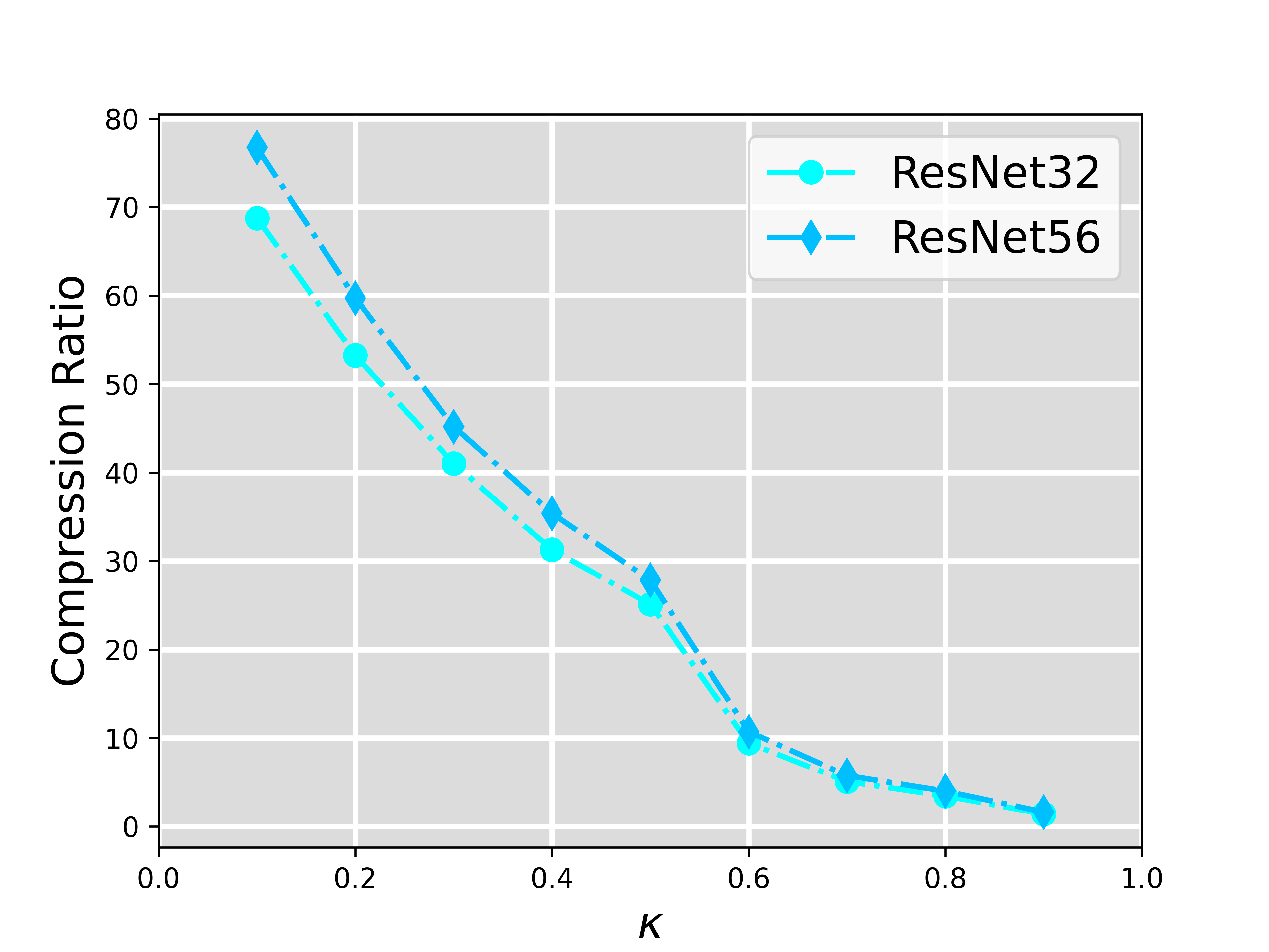
(c) Compression Ratio

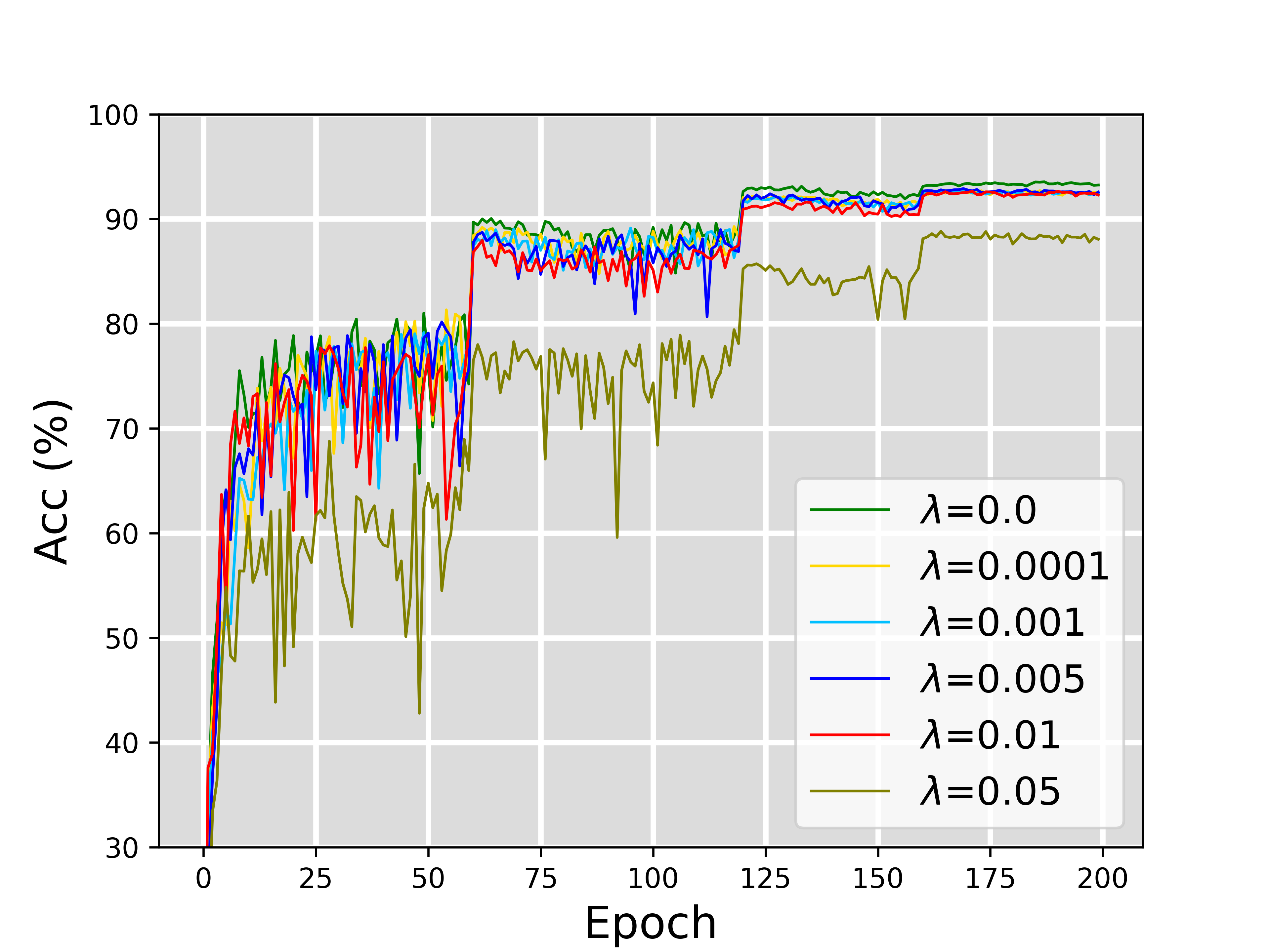
(d) Training Acc.

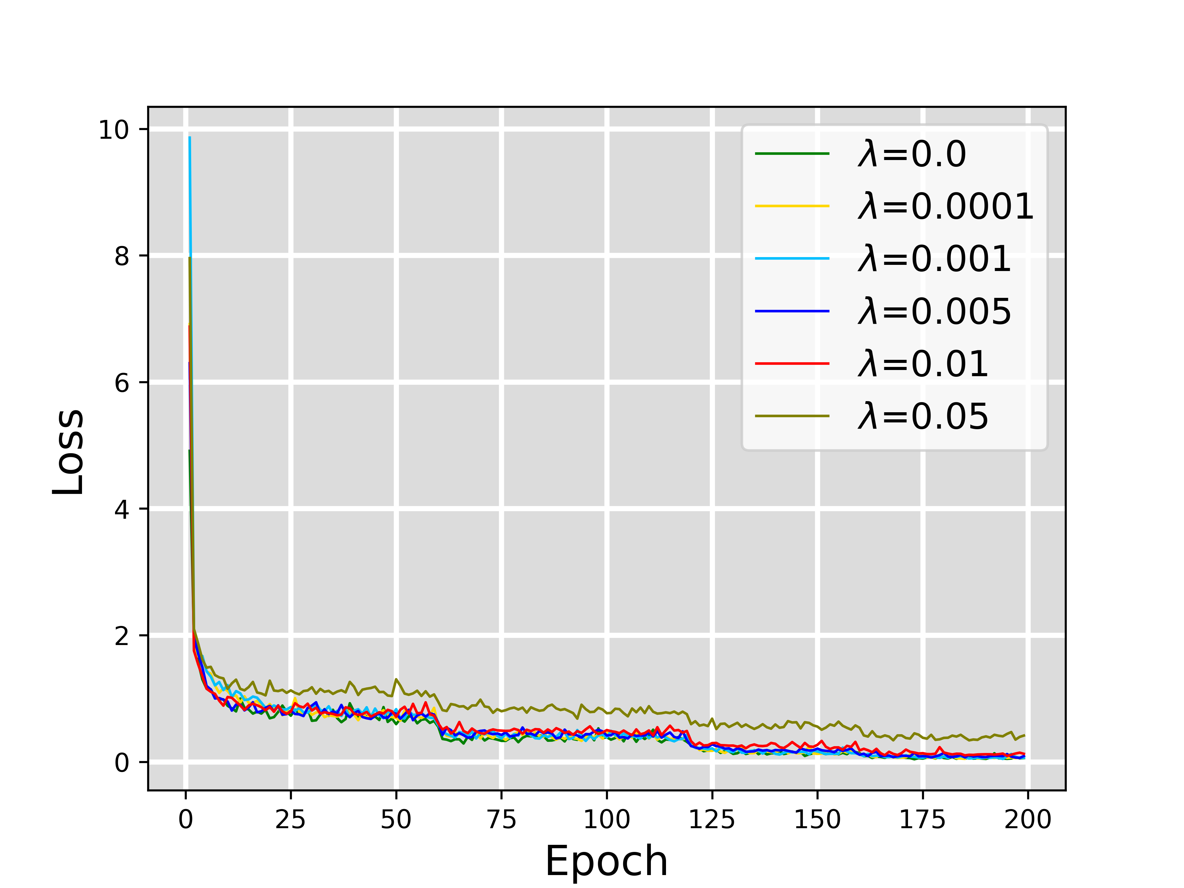
(e) Training Loss

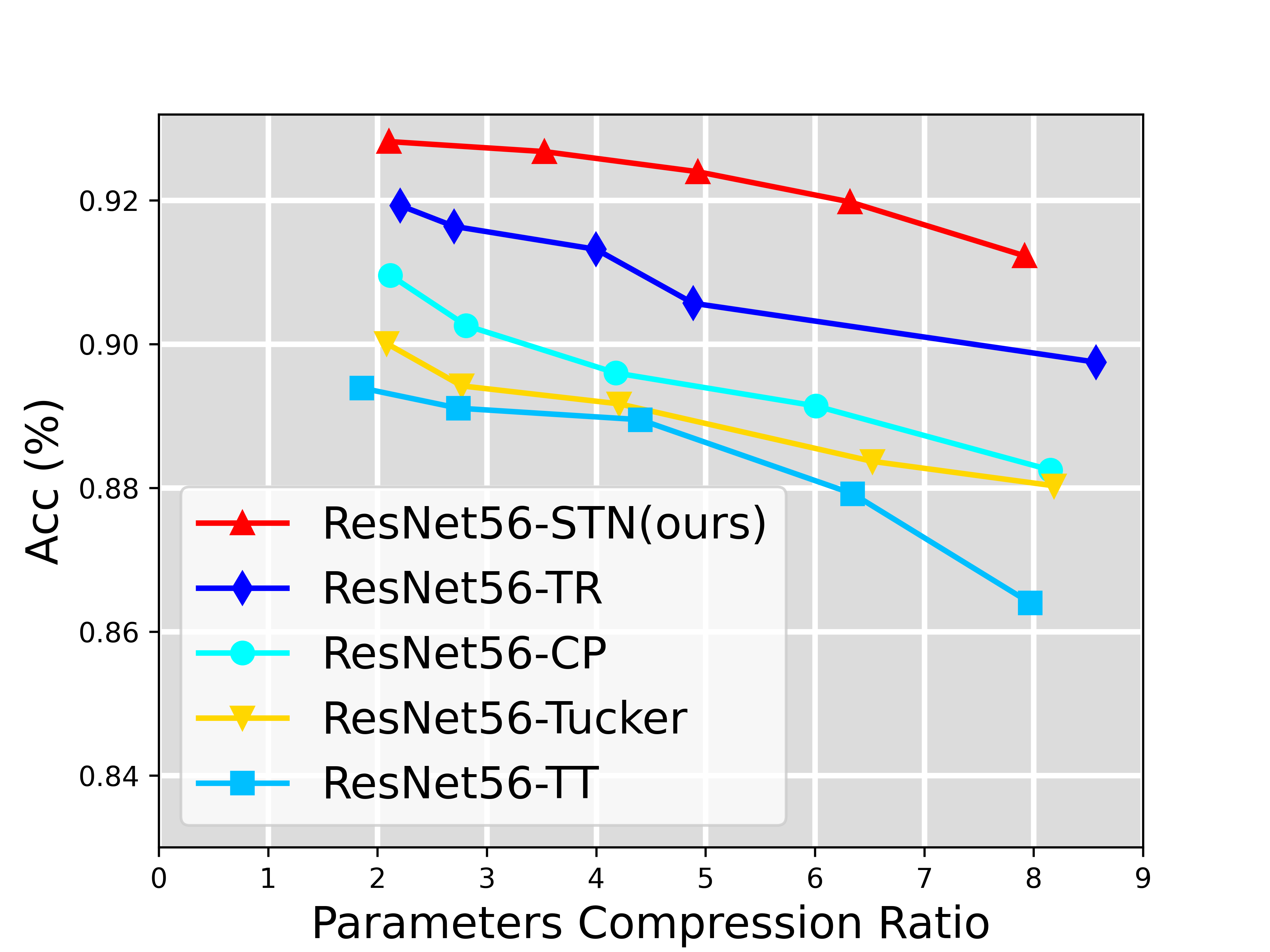
(f) Compression vs. Acc.

Figure 3: Ablation study with ResNet-56 on CIFAR10. (a) Compression ratios of 54 convolutional layers under different $\kappa$ in decomposition stage. (b) Approximate relative square error (RSE) of convolutional layers of ResNet-56-STN with 4$\times$ compression. (c) Trade-off curve between model redunction ratios and $\kappa$. (d), (e) Test accuracy and training loss during structure-aware training stage with different $\lambda$. (f) Trade-off curves of accuracy vs. parameters compression ratio for TD-based ResNet-56 model.

4 Experiments

To validate the effectiveness of our methods, we conduct compression experiments on several popular architectures with different tasks. We apply our compression model on the ResNet family [14] for image classification tasks and report its validation accuracy on CIFAR10 [21] and ImageNet datasets [36]. For the image segmentation task, we perform compression on the renowned U-Net architecture [35] and evaluate the performance on the medical Lung-CXR dataset [17]. In comparison, we evaluated other TD and quantization strategies-based networks on the same baselines, and other scalable approaches. For fairness, our experiments follow the same setups as [49, 37].

4.1 Ablation Study

The tuning parameter $\kappa$ in (11) controls the computational complexity and performance of STN during its compression stage. Note that we only use $\kappa$ to manipulate the size of the target model instead of manually designing the decomposition rank for each layer separately, which greatly simplifies the resizing of the model. After that, we experimentally reveal that different layers of a DNN model can exhibit various low-rank behaviours. As shown in Fig. 3(a), it displays the compression ratio of 54 convolutional layers inside BasicBlock of ResNet-56 under $\kappa$ of 0.5, 0.7, and 0.9, respectively. We can observe that different layers present significant compression differences even at the same $\kappa$, e.g., the 26th and 41st layers achieve 22$\times$ and 60$\times$ compression, respectivel, at $\kappa=0.5$. Further, we visualize the RSE per convolutional layers of Resnet-56 in Fig. 3(b), where the compression ratios per layer are similar. It can be observed that the degree of approximation varies significantly among layers, which further provides empirical evidence that different layers exhibit apparent low-rankness behaviour inconsistencies across networks. Therefore, it is appropriate to select adaptive TN-ranks for each layer compression based on the intrinsic properties of the weight tensors, which enables us to reconfigure the model more flexibly and efficiently.

Next, we analyze the influence of the parameter $\lambda$ in (3) on the model performance and convergence during the structure-aware training process of STN. As shown in Fig. 3(d), which illustrates the validation accuracy curves under different $\lambda$ of ResNet-56. We notice that the regularized model exhibits similar performance when $\lambda\leq 0.01$. In addition, the setting of $\lambda$ barely affects the training convergence of the regularized ResNet-56 (see Fig. 3(e)). The accuracy of the network, however, decreases rapidly when $\lambda=0.05$, attributed to the fact that the excessively low-rank constraint bounds the model’s fitting capability. In order to obtain a simultaneous low-rank and high-accuracy model, we choose $\lambda=0.005$ in the subsequent experiments.

Table 1: Performance comparison of various methods based on TD and pruning strategies in compressing ResNet-18 on ImageNet. $\downarrow$ denotes compression ratio.

Method	Strategy	FLOPs $\downarrow$	Top-5 (%)
ResNet-18(baseline) [14]	-	1.0 $\times$	88.94
DACP-ResNet-18 [55]	Pruning	1.9 $\times$	87.60
FBS-ResNet-18 [8]		2.0 $\times$	88.22
FPGM-ResNet-18 [15]		1.7 $\times$	88.53
DSA-ResNet-18 [28]		1.7 $\times$	88.35
STN-ResNet-18 (ours)		2.3 $\times$	88.65
SVD-ResNet-18 [44]	TD	3.2 $\times$	86.61
TT-ResNet-18 [9]		4.6 $\times$	85.64
TR-ResNet-18 [41]		4.3 $\times$	86.29
STN-ResNet-18 (ours)		4.5 $\times$	87.86

Table 2: Performance comparison in compressing U-Net on Lung-CXR. The evaluation indexes include the compression ratio of parameters (CR) and FLOPs, respectively, as well as the area under the precision-recall curve (PRAUC).

Method	CR	FLOPs $\downarrow$	PRAUC(%)
U-Net(baseline) [35]	1.0$\times$	1.0$\times$	98.2
DSC-U-Net [4]	7.9$\times$	5.2$\times$	97.1
CP-U-Net [24]	6.1$\times$	4.2$\times$	97.4
Tucker-U-Net [18]	6.9$\times$	4.6$\times$	96.4
TT-U-Net [9]	5.8$\times$	4.0$\times$	97.5
TR-U-Net [41]	7.0$\times$	5.1$\times$	97.8
STN-U-Net (ours)	6.5$\times$	5.5$\times$	98.0

4.2 Comparison with Compression Methods

In this part, we compare STN with other one-shot compression methods and conduct experiments on several benchmarks. For the fair competition, all tensorized networks are trained from scratch to verify the superiority of adaptive TN decomposition.

CIFAR10. We compare STN with other TD methods, including Tucker, CP, TT, and TR decomposition [24, 18, 9, 41]. Figure 3(f) plots the trade-off curves of accuracy versus parameters compression ratio for TD-based ResNet-56. Note here we only decompose the convolutional layers since the number of parameters in fully-connected layers is negligible. ResNet-56-STN can achieve higher accuracy with less storage cost, whereas other TD methods lead to significant performance degradation. For instance, even for the advanced TT and TR decompositions, they cause 3.9% and 1.7% accuracy loss of ResNet-56 at 4.4$\times$ and 4.0$\times$ compression, respectively. Surprisingly, our method achieves 4.1$\times$ and 3.5$\times$ parameters reduction on compressing ResNet-56 with only 0.6% and 0.3% performance degradation. This indicates that our adaptive approach achieves higher compression ratios and better performance than other TD methods.

ImageNet. Next, we conduct experiments on the large benchmark dataset ImageNet and report the experimental results of various TD- and pruning strategy-based methods towards compressing ResNet-18 in Table 1. Here we decompose the convolutional and fully-connected layers of ResNet-18 under $\kappa=0.8$, and obtain 4.5$\times$ FLOPs reduction at the expense of 1.08% accuracy loss. Consequently, STN can achieve higher accuracy with similar parameters than TD-based methods and construct compacter parameter spaces compared with pruning-based methods. This experiment further demonstrates the superiority of STN, i.e., exploring the low-rank structure of each layer of the weight tensor to maximize compression.

Lung-CXR. We validate the generalization ability of STN on the image segmentation task. As shown in Table 2, we employ various TD methods and depthwise separable convolution (DSC) [4] to compress the prominent U-Net architecture [35]. The STN achieves 6.5$\times$ compression and best segmentation performance with the cost of 0.2% drop of PRAUC. On the other hand, we avoid the hassle of setting the TN-ranks for each layer. Therefore, STN is more suitable for resizing the model flexibly and achieving better performance.

4.3 Comparison with Scalable Networks

We have demonstrated the superiority of adaptive decomposition in the previous experiments. Here, we further show the effectiveness of structure-aware training of STN. As shown in Fig.4, direct compressing the routinely trained full-rank ResNet-32 via Algorithm 2 leads to rapidly decreasing accuracy. In contrast, STN performing approximation on the low-rank model can maintain model performances well in a wide range. In particular, the model accuracy drops by only 0.9% at a compression ratio of 2.1$\times$ (Table 3). It implies that introducing an additional low-rank regularizer during the training procedure can guarantee the desired low-rank characteristics of the network, thus effectively reducing the approximation error induced in the post-processing stage. More strikingly, the SVD-based Tucker decomposition with the variational Bayesian matrix factorization (VBMF) rank determination strategy performs even worse than the routinely trained STN. That hints iteratively decomposing the convolution kernel with the ALS algorithm has a lower RSE. Finally, the results in Table 4 further evidence the advantage of STN in inference speed.

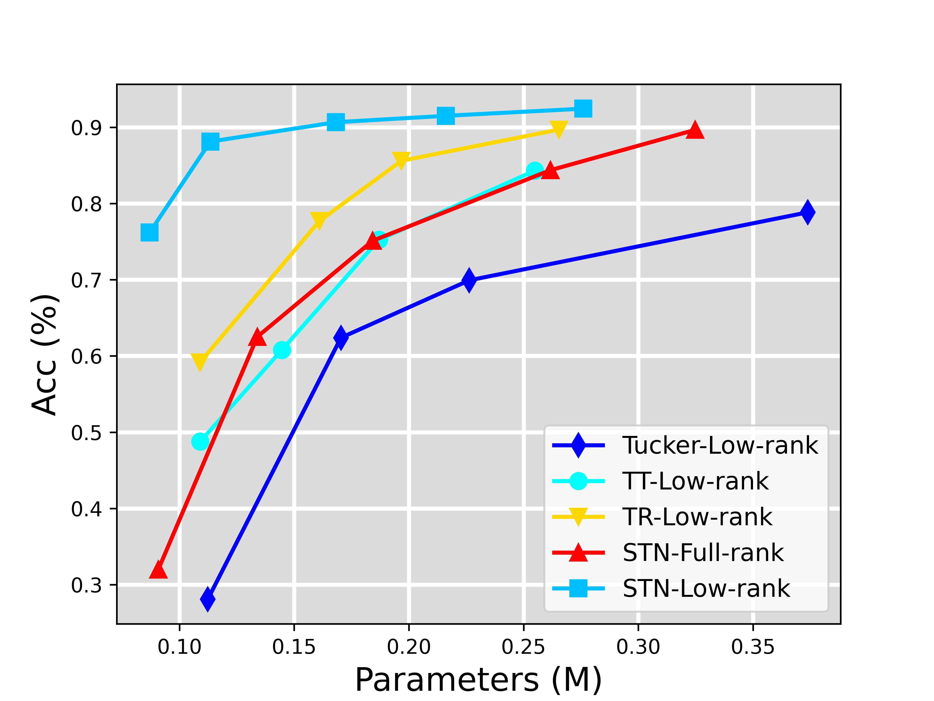
Figure 4: Scalable compression results with ResNet-32 on the CIFAR10 datasets.

Table 3: Performance comparison of various TD methods in compressing ResNet-32 without fine-tuning.

Method	CR	FLOPs $\downarrow$	Top-1 (%)
ResNet-32(baseline) [14]	1.0$\times$	1.0$\times$	92.5
Tucker-Low-rank [18]	1.3$\times$	1.5$\times$	78.8
TT-Low-rank[9]	1.8$\times$	1.8$\times$	84.3
TR-Low-rank [41]	1.7$\times$	2.0$\times$	89.7
STN-Full-rank (ours)	1.8$\times$	1.9$\times$	84.4
STN-Low-rank (ours)	2.1$\times$	2.5$\times$	91.6

Figure 5: Visualization of topologies and TN-ranks for compressing the 2nd, 6th, 10th, 14th, and 18th layers of ResNet-18 via TT, TR, and STN ($\kappa=0.7$). Note that TT and TR have fixed structures and manually determined ranks. The front four graphics correspond to convolutional layers, and the last one refers to fully-connected layers.

Table 4: Comparison of inference speed (Intel-Xeon 6226R CPU) per image with ResNet-56 on the CIFAR10 datasets.

Method	Top-1 (%)	Time (ms)	Speed
ResNet-56 (baseline) [14]	92.5	4.22	1.00 $\times$
CP-ResNet-56 [24]	90.26	2.86	1.47 $\times$
Tucker-ResNet-56 [24]	90.03	2.06	2.05 $\times$
TT-ResNet-56 [24]	89.39	3.47	1.22 $\times$
TR-ResNet-56 [24]	90.57	2.90	1.45 $\times$
STN-ResNet-56 (ours)	91.23	1.83	2.31 $\times$

Table 5: Performance comparison of various scalable methods in compressing ResNet-18 on ImageNet.

Method	Top-1 (%)	Top-5 (%)	CR
ResNet-18(baseline) [14]	69.10	88.94 $\times$	1.0 $\times$
TRP1+Nu [44]	65.39	86.37	2.2 $\times$
$[$Jaderberg $et\ al$.$]$ [16]	62.80	83.72	2.0 $\times$
$[$Zhang $et\ al$.$]$ [52]	63.10	84.44	1.4 $\times$
Slimmable-net [50]	66.52	87.12	1.9 $\times$
Decomposable-net [47]	67.14	87.30	2.3 $\times$
STN (ours)	67.85	88.03	2.2 $\times$

We compare STN with other scalable methods, including TRP [44] , Slimmable networks [50], and Decomposable-net [47]. Table 5 reports the performance of various approaches towards compressing ResNet-18 on ImageNet. Obviously, STN achieves the best 67.85% classification accuracy with 2.2$\times$ compression. Compared to TRP, the precision is 2.46 higher at the same compression ratio. This implies that the STN trained under the ADMM framework possesses low-rank characteristics and facilitates the subsequent adaptive decomposition. More interestingly, we visualize the decomposed topological structures and TN-ranks of several convolutional and the fully-connected layers of ResNet-18 in Fig. 6, and it is evident that the adaptiveness of STN includes two parts: decomposition mode and rank selection. Also, we can see the intensity of the mode correlation of the weight tensors according to the magnitude of the edge rank between the connected factors; for example, the correlation between the channel modes of convolution kernels is stronger than the spatial ones. Moreover, the topological structure easily forms a fully-connected graph for the fully-connected layer due to its balanced mode dimension. In conclusion, the adaptive compression of the weight parameters and the low-rank structure-aware training is crucial for the success of the STN.

5 Conclusion

We propound the Scalable Tensorizing Networks (STN) to improve parameter efficiency and scalability of neural networks. First, we introduce a low-rank regularizer during the training of the DNN model and develop a structure-aware training algorithm, which can effectively reduce the approximation error of the decomposition and thus avoid the subsequent retraining stage. After that, recognizing that different layers exhibit various low-rank behaviours and ALS-based adaptive compression strategy is adopted to compress the convolutional and fully-connected layers simultaneously. Comprehensive experiments on multiple network architectures substantiate the superiority and effectiveness of our approach over other state-of-the-art low-rank and scalable networks.

6 Appendix

6.1 Analysis

We report the storage and calculation complexity for different methods against compressed convolutional and fully-connected layers in Tables 1 and 2. Note that the CP and Tucker decompositions are not suited for fully-connected layer compression. Despite the higher theoretical complexity of our STN, empirical evidence in the main paper has revealed that adaptive compression is more advantageous in dealing with mode-unbalanced low-order tensors, and the compressed DNNs achieve higher performance. In addition, the split dimension in the tensorization process obeys the variance minimization principle.

Table 6: Comparison of parameters and FLOPs involved in convolutional layer compressed by different methods.

Methods	Parameters	FLOPs
Conv (Standard)	$K^{2}\times S\times T$	$K^{2}\times S\times T\times W\times H$
DSC [4]	$(K^{2}+T)\times S$	$(K^{2}+T)\times S\times W\times H$
CP [24]	$R_{cp}(S+T+2K)$	$R_{cp}(C+D+2K)\times W\times H$
Tucker [18]	$R_{Tuc}(S+T)+R_{Tuc}^{2}K^{2}$	$R_{Tuc}(C+D+R_{Tuc}K^{2})\times W\times H$
TT [9]	$(S+T+2KR_{TT})R_{TT}$	$(S+T+K^{2}R_{TT})R_{TT}\times W\times H+K^{2}R_{TT}^{3}$
TR [41]	$(S+T+2K)R_{TR}^{2}$	$(S+T+K^{2}R_{TR}^{2})R_{TR}^{2}\times W\times H+K^{2}R_{TR}^{4}$
STN (ours)	$(S+T+2K)R_{TN}^{3}$	$(S+T+K^{2}R_{TN}^{2})R_{TN}^{3}\times W\times H+K^{2}R_{TN}^{5}$

Table 7: Comparison of parameters and FLOPs involved in fully-connected layer compressed by different methods. The weight matrix $\boldsymbol{W}\in\mathbb{R}^{M\times N}$ and $M=I_{1}I_{2},N=J_{1}J_{2}$.

Methods	Parameters	FLOPs
FC (Standard)	$I_{1}I_{2}\times J_{1}J_{2}$	$I_{1}I_{2}\times J_{1}J_{2}\times C$
TT [9]	$(I_{1}+J_{2})R_{TT}+(I_{2}+J_{1})R_{TT}^{2}$	$(I_{1}I_{2}+J_{1}J_{2})R_{TT}\times(C+R_{TT})$
TR [41]	$(I_{1}+I_{2}+J_{1}+J_{2})R_{TR}^{2}$	$(I_{1}I_{2}+J_{1}J_{2})R_{TT}^{2}\times(C+R_{TT})$
STN (ours)	$(I_{1}+I_{2}+J_{1}+J_{2})R_{TN}^{3}$	$(I_{1}I_{2}+J_{1}J_{2})R_{TN}^{3}\times(C+R_{TN}^{2})$

The storage and computation complexity of TD-based compression is closely related to the rank selection, and we hereby reveal the relationship between the TN-rank with the CP and Tucker ranks in Theorem 1.

Theorem 1.  Consider an $N$th-order tensor $\boldsymbol{\mathcal{X}}\in\mathbb{R}^{I_{1}\times\dots\times I_{N}}$ can be represented in TN-format. Then we have: (1) If $\boldsymbol{\mathcal{X}}$ has CP rank $R_{cp}$, then $rank(\boldsymbol{X}_{[n_{1:r};n_{r+1:N}]})\leq\min\{\prod_{i=1}^{r}\prod_{j=r+1}^{N}R_{n_{i},n_{j}},R_{cp}\}$. (2) If $\boldsymbol{\mathcal{X}}$ has Tucker rank $R_{Tuc}=(r_{1},\cdots,r_{N})$, then $rank(\boldsymbol{X}_{[n_{1:r};n_{r+1:d}]})\leq\min\{\prod_{i=1}^{r}r_{n_{i}},\prod_{j=r+1}^{N}r_{n_{j}}\}$,, where $\boldsymbol{X}_{[n_{1:r};n_{r+1:d}]}\in\mathbb{R}^{I_{n_{1}}\dots I_{n_{r}}\times I_{n_{r+1}}\dots I_{n_{N}}}$.

6.2 More experimental results

We illustrate the trade-off curve of STN towards compressing ResNet-50 on the CIFAR100 datasets in Figure 1. Compared with the TR-based compression (TR-ResNet-50) and trained rank pruning (STN-ResNet-50) method [44], the experimental results further validate the superiority of adaptive compression and scalable strategies.

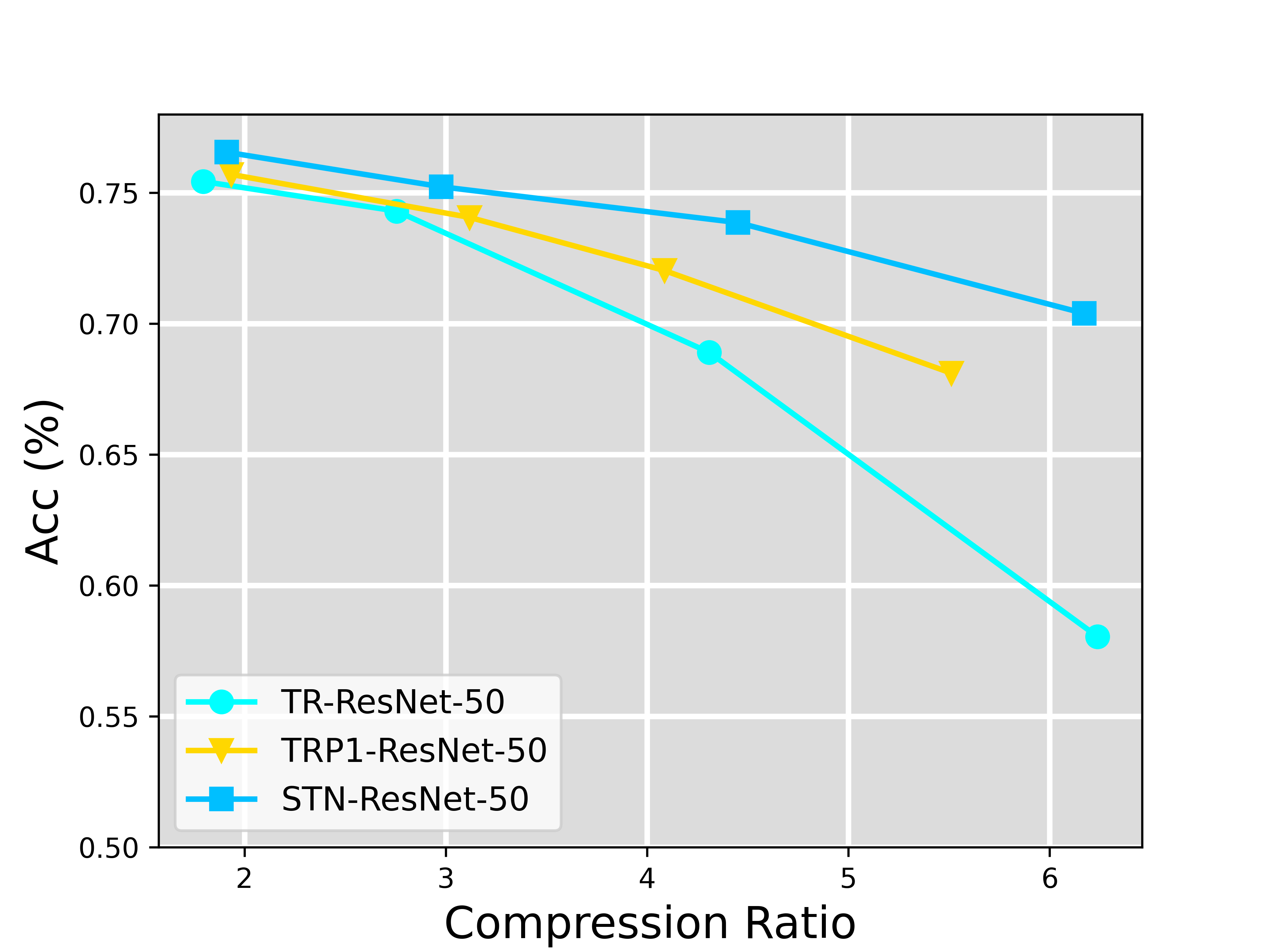
Figure 6: Scalable compression results with ResNet-50 on the CIFAR100 datasets. Our STN-ResNet50 consistently achieves the best performance at varying parameter compression ratios

References

- [1] Jose M Alvarez and Mathieu Salzmann. Compression-aware training of deep networks. Advances in neural information processing systems, 30:856–867, 2017.
- [2] Stephen Boyd, Neal Parikh, Eric Chu, Borja Peleato, and Jonathan Eckstein. Distributed Optimization and Statistical Learning Via the Alternating Direction Method of Multipliers. 2011.
- [3] Xinlei Chen, Ross Girshick, Kaiming He, and Piotr Dollár. Tensormask: A foundation for dense object segmentation. In Proceedings of the IEEE/CVF International Conference on Computer Vision, pages 2061–2069, 2019.
- [4] François Chollet. Xception: Deep learning with depthwise separable convolutions. In Proceedings of the IEEE conference on computer vision and pattern recognition, pages 1251–1258, 2017.
- [5] Andrzej Cichocki, Danilo Mandic, Lieven De Lathauwer, Guoxu Zhou, Qibin Zhao, Cesar Caiafa, and Huy Anh Phan. Tensor decompositions for signal processing applications: From two-way to multiway component analysis. IEEE signal processing magazine, 32(2):145–163, 2015.
- [6] Emily L Denton, Wojciech Zaremba, Joan Bruna, Yann LeCun, and Rob Fergus. Exploiting linear structure within convolutional networks for efficient evaluation. In Advances in neural information processing systems, pages 1269–1277, 2014.
- [7] Simon Du and Jason Lee. On the power of over-parametrization in neural networks with quadratic activation. In International Conference on Machine Learning, pages 1329–1338. PMLR, 2018.
- [8] Xitong Gao, Yiren Zhao, Łukasz Dudziak, Robert Mullins, and Cheng-zhong Xu. Dynamic channel pruning: Feature boosting and suppression. arXiv preprint arXiv:1810.05331, 2018.
- [9] Timur Garipov, Dmitry Podoprikhin, Alexander Novikov, and Dmitry Vetrov. Ultimate tensorization: compressing convolutional and fc layers alike. arXiv preprint arXiv:1611.03214, 2016.
- [10] Ian Goodfellow, Jean Pouget-Abadie, Mehdi Mirza, Bing Xu, David Warde-Farley, Sherjil Ozair, Aaron Courville, and Yoshua Bengio. Generative adversarial nets. Advances in neural information processing systems, 27, 2014.
- [11] Song Han, Huizi Mao, and William J Dally. Deep compression: Compressing deep neural networks with pruning, trained quantization and huffman coding. arXiv preprint arXiv:1510.00149, 2015.
- [12] Richard A Harshman et al. Foundations of the parafac procedure: Models and conditions for an” explanatory” multimodal factor analysis. 1970.
- [13] Kaiming He, Georgia Gkioxari, Piotr Dollár, and Ross Girshick. Mask r-cnn. In Proceedings of the IEEE international conference on computer vision, pages 2961–2969, 2017.
- [14] Kaiming He, Xiangyu Zhang, Shaoqing Ren, and Jian Sun. Deep residual learning for image recognition. In Proceedings of the IEEE conference on computer vision and pattern recognition, pages 770–778, 2016.
- [15] Yang He, Ping Liu, Ziwei Wang, Zhilan Hu, and Yi Yang. Filter pruning via geometric median for deep convolutional neural networks acceleration. In Proceedings of the IEEE/CVF Conference on Computer Vision and Pattern Recognition, pages 4340–4349, 2019.
- [16] Max Jaderberg, Andrea Vedaldi, and Andrew Zisserman. Speeding up convolutional neural networks with low rank expansions. arXiv preprint arXiv:1405.3866, 2014.
- [17] Stefan Jaeger, Sema Candemir, Sameer Antani, Yì-Xiáng J Wáng, Pu-Xuan Lu, and George Thoma. Two public chest x-ray datasets for computer-aided screening of pulmonary diseases. Quantitative imaging in medicine and surgery, 4(6):475, 2014.
- [18] Yong-Deok Kim, Eunhyeok Park, Sungjoo Yoo, Taelim Choi, Lu Yang, and Dongjun Shin. Compression of deep convolutional neural networks for fast and low power mobile applications. arXiv preprint arXiv:1511.06530, 2015.
- [19] Tamara G Kolda and Brett W Bader. Tensor decompositions and applications. SIAM review, 51(3):455–500, 2009.
- [20] Jean Kossaifi, Adrian Bulat, Georgios Tzimiropoulos, and Maja Pantic. T-net: Parametrizing fully convolutional nets with a single high-order tensor. In Proceedings of the IEEE/CVF Conference on Computer Vision and Pattern Recognition, pages 7822–7831, 2019.
- [21] Alex Krizhevsky, Geoffrey Hinton, et al. Learning multiple layers of features from tiny images. 2009.
- [22] Alex Krizhevsky, Ilya Sutskever, and Geoffrey E Hinton. Imagenet classification with deep convolutional neural networks. Advances in neural information processing systems, 25:1097–1105, 2012.
- [23] Nicholas D Lane, Sourav Bhattacharya, Petko Georgiev, Claudio Forlivesi, and Fahim Kawsar. An early resource characterization of deep learning on wearables, smartphones and internet-of-things devices. In Proceedings of the 2015 international workshop on internet of things towards applications, pages 7–12, 2015.
- [24] Vadim Lebedev, Yaroslav Ganin, Maksim Rakhuba, Ivan Oseledets, and Victor Lempitsky. Speeding-up convolutional neural networks using fine-tuned cp-decomposition. arXiv preprint arXiv:1412.6553, 2014.
- [25] Cun Mu, Bo Huang, John Wright, and Donald Goldfarb. Square deal: Lower bounds and improved relaxations for tensor recovery. In International conference on machine learning, pages 73–81. PMLR, 2014.
- [26] Chang Nie, Huan Wang, and Zhihui Lai. Multi-tensor network representation for high-order tensor completion. arXiv preprint arXiv:2109.04022, 2021.
- [27] Chang Nie, Huan Wang, and Le Tian. Adaptive tensor networks decomposition. In BMVC, 2021.
- [28] Xuefei Ning, Tianchen Zhao, Wenshuo Li, Peng Lei, Yu Wang, and Huazhong Yang. Dsa: More efficient budgeted pruning via differentiable sparsity allocation. In Computer Vision–ECCV 2020: 16th European Conference, Glasgow, UK, August 23–28, 2020, Proceedings, Part III 16, pages 592–607. Springer, 2020.
- [29] Alexander Novikov, Dmitry Podoprikhin, Anton Osokin, and Dmitry Vetrov. Tensorizing neural networks. arXiv preprint arXiv:1509.06569, 2015.
- [30] Román Orús. A practical introduction to tensor networks: Matrix product states and projected entangled pair states. Annals of Physics, 349:117–158, 2014.
- [31] Ivan V Oseledets. Tensor-train decomposition. SIAM Journal on Scientific Computing, 33(5):2295–2317, 2011.
- [32] Yu Pan, Jing Xu, Maolin Wang, Jinmian Ye, Fei Wang, Kun Bai, and Zenglin Xu. Compressing recurrent neural networks with tensor ring for action recognition. In Proceedings of the AAAI Conference on Artificial Intelligence, volume 33, pages 4683–4690, 2019.
- [33] Joseph Redmon, Santosh Divvala, Ross Girshick, and Ali Farhadi. You only look once: Unified, real-time object detection. In Proceedings of the IEEE conference on computer vision and pattern recognition, pages 779–788, 2016.
- [34] Shaoqing Ren, Kaiming He, Ross Girshick, and Jian Sun. Faster r-cnn: Towards real-time object detection with region proposal networks. Advances in neural information processing systems, 28:91–99, 2015.
- [35] Olaf Ronneberger, Philipp Fischer, and Thomas Brox. U-net: Convolutional networks for biomedical image segmentation. In International Conference on Medical image computing and computer-assisted intervention, pages 234–241. Springer, 2015.
- [36] Olga Russakovsky, Jia Deng, Hao Su, Jonathan Krause, Sanjeev Satheesh, Sean Ma, Zhiheng Huang, Andrej Karpathy, Aditya Khosla, Michael Bernstein, et al. Imagenet large scale visual recognition challenge. International journal of computer vision, 115(3):211–252, 2015.
- [37] Raghavendra Selvan, Erik B Dam, and Jens Petersen. Segmenting two-dimensional structures with strided tensor networks. In International Conference on Information Processing in Medical Imaging, pages 401–414. Springer, 2021.
- [38] Mahdi Soltanolkotabi, Adel Javanmard, and Jason D Lee. Theoretical insights into the optimization landscape of over-parameterized shallow neural networks. IEEE Transactions on Information Theory, 65(2):742–769, 2018.
- [39] Ledyard R Tucker. Some mathematical notes on three-mode factor analysis. Psychometrika, 31(3):279–311, 1966.
- [40] Michael E Wall, Andreas Rechtsteiner, and Luis M Rocha. Singular value decomposition and principal component analysis. In A practical approach to microarray data analysis, pages 91–109. Springer, 2003.
- [41] Wenqi Wang, Yifan Sun, Brian Eriksson, Wenlin Wang, and Vaneet Aggarwal. Wide compression: Tensor ring nets. In Proceedings of the IEEE Conference on Computer Vision and Pattern Recognition, pages 9329–9338, 2018.
- [42] Wei Wen, Chunpeng Wu, Yandan Wang, Yiran Chen, and Hai Li. Learning structured sparsity in deep neural networks. Advances in neural information processing systems, 29:2074–2082, 2016.
- [43] Bijiao Wu, Dingheng Wang, Guangshe Zhao, Lei Deng, and Guoqi Li. Hybrid tensor decomposition in neural network compression. Neural Networks, 132:309–320, 2020.
- [44] Yuhui Xu, Yuxi Li, Shuai Zhang, Wei Wen, Botao Wang, Wenrui Dai, Yingyong Qi, Yiran Chen, Weiyao Lin, and Hongkai Xiong. Trained rank pruning for efficient deep neural networks. In 2019 Fifth Workshop on Energy Efficient Machine Learning and Cognitive Computing-NeurIPS Edition (EMC2-NIPS), pages 14–17. IEEE, 2019.
- [45] Yuhui Xu, Yuxi Li, Shuai Zhang, Wei Wen, Botao Wang, Yingyong Qi, Yiran Chen, Weiyao Lin, and Hongkai Xiong. Trp: Trained rank pruning for efficient deep neural networks. arXiv preprint arXiv:2004.14566, 2020.
- [46] Yuhui Xu, Yongzhuang Wang, Aojun Zhou, Weiyao Lin, and Hongkai Xiong. Deep neural network compression with single and multiple level quantization. In Proceedings of the AAAI Conference on Artificial Intelligence, volume 32, 2018.
- [47] Atsushi Yaguchi, Taiji Suzuki, Shuhei Nitta, Yukinobu Sakata, and Akiyuki Tanizawa. Decomposable-net: Scalable low-rank compression for neural networks. arXiv preprint arXiv:1910.13141, 2019.
- [48] Yinchong Yang, Denis Krompass, and Volker Tresp. Tensor-train recurrent neural networks for video classification. In International Conference on Machine Learning, pages 3891–3900. PMLR, 2017.
- [49] Miao Yin, Yang Sui, Siyu Liao, and Bo Yuan. Towards efficient tensor decomposition-based dnn model compression with optimization framework. In Proceedings of the IEEE/CVF Conference on Computer Vision and Pattern Recognition, pages 10674–10683, 2021.
- [50] Jiahui Yu, Linjie Yang, Ning Xu, Jianchao Yang, and Thomas Huang. Slimmable neural networks. arXiv preprint arXiv:1812.08928, 2018.
- [51] Tianyun Zhang, Shaokai Ye, Kaiqi Zhang, Jian Tang, Wujie Wen, Makan Fardad, and Yanzhi Wang. A systematic dnn weight pruning framework using alternating direction method of multipliers. In Proceedings of the European Conference on Computer Vision (ECCV), pages 184–199, 2018.
- [52] Xiangyu Zhang, Jianhua Zou, Kaiming He, and Jian Sun. Accelerating very deep convolutional networks for classification and detection. IEEE transactions on pattern analysis and machine intelligence, 38(10):1943–1955, 2015.
- [53] Yi Zhang, Yu Zhang, and Wei Wang. Multi-task learning via generalized tensor trace norm. In Proceedings of the 27th ACM SIGKDD Conference on Knowledge Discovery & Data Mining, pages 2254–2262, 2021.
- [54] Qibin Zhao, Guoxu Zhou, Shengli Xie, Liqing Zhang, and Andrzej Cichocki. Tensor ring decomposition. arXiv preprint arXiv:1606.05535, 2016.
- [55] Zhuangwei Zhuang, Mingkui Tan, Bohan Zhuang, Jing Liu, Yong Guo, Qingyao Wu, Junzhou Huang, and Jinhui Zhu. Discrimination-aware channel pruning for deep neural networks. arXiv preprint arXiv:1810.11809, 2018.