Abstract

We introduce a nonlinear, one-dimensional bending-twisting model for an inextensible bi-rod that is composed of a nematic liquid crystal elastomer. The model combines an elastic energy that is quadratic in curvature and torsion with a Frank-Oseen energy for the liquid crystal elastomer. Moreover, the model features a nematic-elastic coupling that relates the crystalline orientation with a spontaneous bending-twisting term. We show that the model can be derived as a $\Gamma$-limit from three-dimensional nonlinear elasticity. Moreover, we introduce a numerical scheme to compute critical points of the bending-twisting model via a discrete gradient flow. We present various numerical simulations that illustrate the rich mechanical behavior predicted by the model. The numerical experiments reveal good stability and approximation properties of the method.

Keywords: dimension reduction, nonlinear elasticity, nonlinear rods, liquid crystal elastomer, constrained finite element method.

MSC-2020: 74B20; 76A15; 74K10; 65N30; 74-10.

1 Introduction

Nematic liquid crystal elastomers (LCE) are nonlinearly elastic materials that feature an additional orientational internal degree of freedom. They are composed of a polymer network with incorporated liquid crystals—rod-like molecules that tend to align in a nematic phase. Nematic LCE feature a nematic-elastic coupling between the orientation of the liquid cyrstals and the elastic properties of the polymer network. More specificially, the material tends to stretch in the direction parallel to the liquid crystal orientation and shrinks in orthogonal directions. Furthermore, it is possible to tweak the orientation of the liquid crystals by fields and to (de)activate the nematic-elastic coupling by external stimuli (e.g., temperature). For this reasons, nematic LCE exhibit interesting mechanical properties (e.g., thermo-mechanical coupling [B_broer11, B_Warner07] or soft elasticity [B_Finkelman91, B_Kundler95]), and are used to design active materials, see [B_White15, ware2016localized, MaJaZa18]. In this context, slender structure such as thin films and rods are of interest. In recent years nonlinear models for thin films and rods made of nematic LCE have also been intensively studied from a mathematical perspective. In particular, the derivation of lower-dimensional models from thee-dimensional models has been discussed, e.g., see [B_conti2002soft, B_conti2002semisoft, B_Plucinsky18, B_plucinsky2018patterning, B_cesana2015effective, B_Agostiniani17plate, B_Agostiniani17platesoft, B_Agostiniani17platehetero, B_Agostiniani17ribbon, bauer2019derivation], and reliable numerical schemes have been developed, e.g., see [BaPa21, bonito2021numerical, BBMN18, BaBoNo17, sander2010geodesic, sander2016numerical, le1992finite, bergou2008discrete] for numerical methods for slender structures, [NoWaZh17, nitschke2020liquid, nochetto2017finite, borthagaray2020structure, walker2020finite] for LCE and director fields, and [bartels2022nonlinear] for models that combination thin-film mechanics and director fields.

Our paper is devoted to the modeling and simulation of nonlinear bi-rods that are composed of nematic LCE and a usual nonlinear elastic material. Starting from a three-dimensional nonlinear model that invokes a standard energy functional from nonlinear elasticity, a Frank-Oseen energy for the LCE material, and a nematic-elastic coupling term, we derive via $\Gamma$-convergence a model for an inextensible rod that is capable to describe large bending and twisting deformations, and a coupling mechanism that relates the local orientation of the LCE with a spontaneous curvature/torsion-term. In contrast to other works, e.g., [goriely2022rod], in our model the director field is not prescribed but an additional degree of freedom of the model; moreover, the derivation is ansatz-free in the sense of $\Gamma$-convergence. It is based on the one hand on the recently introduced approach in [bartels2022nonlinear] where the derivation of nematic LCE plates is studied, and on the other hand, on [neukamm2012rigorous, bauer2019derivation] where the simultaneous homogenization and dimension reduction of prestrained rods is analyzed as an extension of the seminal work [mora2002derivation].

Our effective one-dimensional description of LCE rods allows for efficient numerical simulations of complex problem settings. We follow [BarRei20] and use standard $C^{0}$ and $C^{1}$ conforming finite element spaces that are subordinated to a partitioning of the straight reference configuration to approximate director fields and the bending deformation, respectively. Geometric constraints such as the conditions for the material frame are imposed at nodes of the partitioning via suitable linearizations and penalty terms. Similarly, the discretization of the unit-length constraint for the director field describing the LCE orientation is imposed at the nodes. We then use a semi-implicit gradient descent method to decrease the one-dimensional energy functional from a given initial state to obtain stationary configurations via sequences of linear problems with simple system matrices. Our experiments show how a periodic bending behaviour can be controlled in a quasi-static setting via a time-dependent external field. Our simulations also illustrate how internal material parameters, that can be changed via external stimuli, affect the bending behavior in the case of compressive, twist-inducing boundary conditions. The numerical experiments reveal good stability and approximation properties of the iterative method and the devised discretization scheme. They lead to meaningful results within minutes for an elementary implementation on standard desktop computers.

The paper is structured as follows. In Section 2 we first introduce the one-dimensional bending-twisting model. We then introduce a three-dimensional nonlinear elasticity model and show that it $\Gamma$-converges to the one-dimensional model, see Section 2.2. The effective coefficients of the one-dimensional depend on the original material, the geometry of the cross-section and the domain occupied by the LCE. In Section 2.3 we present their definition and derive simplified formulas that hold in special settings. In Section 3 we introduce a discretization of the one-dimensional model minimization problem via a discrete gradient flow, and we explore the model via numerical simulations. All proofs are presented in Section LABEL:S:proof.

2 A bi-rod model for nematic LCEs and its derivation

In this section we introduce a one-dimensional bending-twisting model that describes an inextensible rod that is composed of a nematic LCE and a nonlinearly elastic material, and we explain its derivation from three-dimensional nonlinear elasticity via $\Gamma$-convergence, see Section 2.2 below.

2.1 The one-dimensional model

We denote by $\omega:=(0,L)$ the reference domain of the rod. We describe a configuration of the rod by a triplet $(y,R,n)$ satisfying

$$y\in H^{2}(\omega;\mathbb{R}^{3}),\qquad R\in H^{1}(\omega;\mathbb{R}^{3\times 3}),\qquad n\in H^{1}(\omega;\mathbb{R}^{3})$$ (1)

$$\text{such that for a.e. $x_{1}\in\omega$, }\partial_{1}y(x_{1})=R(x_{1})e_{1},\quad R(x_{1})\in\operatorname{SO}(3),\quad|n(x_{1})|=1.$$

Here, $y$ describes the deformation of the rod and $R$ the deformation of an associated orthonormal frame. The field $n$ describes the orientation of the liquid crystals in global coordinates. We denote by

$$\mathcal{A}:=\{(y,R,n)\,:\,(y,R,n)\text{ satisfies }\eqref{def:rodconf}\,\}$$

the set of all rod configurations and call a pair $(y,R)$ satisfying (1) a framed curve. We consider the energy functional $\mathcal{E}:\mathcal{A}\to\mathbb{R}$ defined by

$$\begin{aligned} \mathcal{E}(y,R,n):=&\int_{\omega}\bar{Q}\Big{(}R^{\top}\partial_{1}R+\bar{r}K_{\operatorname{\rm pre}}(\tfrac{1}{3}I-\hat{n}\otimes\hat{n})\Big{)}+\bar{r}^{2}E_{\operatorname{\rm res}}\big{(}\tfrac{1}{3}I-\hat{n}\otimes\hat{n})\big{)}\,dx_{1}\\ &+\boldsymbol{\kappa}{}^{2}\int_{\omega}|\partial_{1}n|^{2}\,dx^{\prime},\qquad\text{where }\hat{n}:=R^{\top}n,\end{aligned}$$ (2)

where

• $\bar{Q}:\mathbb{R}^{3\times 3}_{\operatorname{\rm skew}}\to\mathbb{R}$ is a positive definite quadratic form that describes the bending–twisting energy; here and below, $\mathbb{R}^{3\times 3}_{\operatorname{\rm skew}}$ denotes the space of skew-symmetric matrices in $\mathbb{R}^{3\times 3}$.

• $K_{\operatorname{\rm pre}}:\mathbb{R}^{3\times 3}_{{\rm dev}}\to\mathbb{R}^{3\times 3}_{\operatorname{\rm skew}}$ is a linear map that describes the contribution of the nematic-elastic coupling that leads to spontaneous bending and twisting of the rod; here and below, $\mathbb{R}^{3\times 3}_{{\rm dev}}$ denotes the space of symmetric matrices in $\mathbb{R}^{3\times 3}$ with vanishing trace.

• $E_{\operatorname{\rm res}}:\mathbb{R}^{3\times 3}_{{\rm dev}}\to\mathbb{R}$ is a positive, semi-definite quadratic form that describes a residual energy that cannot be accomodated by bending or twisting of the rod.

• $\bar{r}\in\mathbb{R}$ is a model parameter related to the strength of the nematic-elastic coupling.

• $\boldsymbol{\kappa}{}>0$ is a model parameter that is related to the scaling of the physical diameter of the rod, the shear moduls of the elastomer and the Frank elastic constant of the nematic LCE.

As we shall explain next, this model can be derived as a zero-thickness $\Gamma$-limit from a three-dimensional rod composed of an elastic material and an LCE-material. In this context, the precise definition of $\bar{Q}$ and $K_{\rm pre}$ depends on the considered material, the geometry of the cross-section of the rod and the geometry of the subdomain that is occupied by the nematic LCE material, see Definition 2.6.

2.2 The three-dimensional model and $\Gamma$-convergence

The starting point of the derivation is the following three-dimensional situation: We consider an elastic composite material that occupies the three-dimensional, rod-like domain $\Omega_{h}:=\omega\times hS$, where $0<h\ll 1$ denotes a (non-dimensionalized) thickness of the rod, $S\subset\mathbb{R}^{2}$ the rescaled cross-section, and $\omega:=(0,L)$ the mide-line of the rod. We assume that

$$S\subset\mathbb{R}^{2}\text{ is a simply connected, Lipschitz domain,}$$ (3)

$$\text{satisfying }\int_{S}x_{2}\,d\bar{x}=\int_{S}x_{3}\,d\bar{x}=\int_{S}x_{2}x_{3}\,d\bar{x}=0.$$

Here and below, we use the notation $x=(x_{1},\bar{x})\in\mathbb{R}^{3}$ and $\bar{x}=(x_{1},x_{2})\in\mathbb{R}^{2}$. We note that the symmetry condition in (3) is not a restriction, since it can always be achieved by rotating and translating $S$. We assume that the rod is composed of a conventional elastic material and a nematic LCE. The latter occupies the subbody $\Omega_{0,h}:=\omega\times(hS_{0})$ where $S_{0}\subset S$ denotes a subdomain of the cross-section. We assume that

$$S_{0}\subset S\text{ is a simply connected, Lipschitz domain such that $|S_{0}|>0$ and $|S\setminus S_{0}|>0$}.$$ (4)

To study the limit $h\to 0$, it is convenient to work with the rescaled domain $\Omega:=\omega\times S$ (resp. the rescaled subdomain $\Omega_{0}:=\omega\times S_{0}$). We therefore describe the deformation of the rod by a mapping $y_{h}:H^{1}(\Omega;\mathbb{R}^{3})$, and the orientation of the LCE by a director field $n_{h}\in H^{1}(\Omega_{0};\mathbb{S}^{2})$. Here and below, $\mathbb{S}^{2}$ denotes unit-sphere in $\mathbb{R}^{3}$. We consider the energy functional

$$\mathcal{E}_{h}(y_{h},n_{h}):= \frac{1}{h^{2}|S|}\int_{\Omega\setminus\Omega_{0}}W\Big{(}\bar{x},\nabla_{h}y_{h}(x)\Big{)}\,dx+\frac{1}{h^{2}|S|}\int_{\Omega_{0}}W\Big{(}\bar{x},L_{h}(n_{h}(x))^{-\frac{1}{2}}\nabla_{h}y_{h}(x)\Big{)}\,dx$$ (5)

$$+\frac{\boldsymbol{\kappa}{}^{2}}{|S_{0}|}\int_{\Omega_{0}}\big{|}\nabla_{h}n_{h}(x)(\nabla_{h}y_{h}(x))^{-1}\big{|}^{2}\det(\nabla_{h}y_{h}(x))\,dx.$$

The first integral is the elastic energy stored in the deformed material with reference configuration $\Omega\setminus\Omega_{0}$. Here, $\nabla_{h}:=(\partial_{1},\frac{1}{h}\bar{\nabla})$, $\bar{\nabla}:=(\partial_{2},\partial_{3})$ denotes the scaled gradient which emerges when passing from $\Omega_{h}$ to $\Omega$. The second integral is the elastic energy of the nematic LCE. It invokes the step-length tensor

$$L_{h}:\mathbb{S}^{2}\to\mathbb{R}^{3\times 3}_{\operatorname{sym}},\qquad L_{h}(n):=(1+h\bar{r})^{-\frac{1}{3}}(I+h\bar{r}n\otimes n),$$

which has been introduced by [bladon1993transitions] to model the elastic-nematic coupling. The last integral is the (one-constant approximation of the) Frank-Oseen energy pulled back to the reference configuration. As already mentioned, $\bar{r}\in\mathbb{R}$ and $\boldsymbol{\kappa}{}>0$ denote model parameters.

We assume that the stored energy function $W:S\times\mathbb{R}^{3\times 3}\to[0,\infty]$ is Borel-measurable and satisfies for some $q>4$ and $C>0$, and for all $F\in\mathbb{R}^{3\times 3}$ and a.e. $\bar{x}\in S$,

$$W(\bar{x},RF)=W(\bar{x},F)\qquad\text{for all }R\in\operatorname{SO}(3),$$ (W1)

$$W(\bar{x},F)\geq\frac{1}{C}\operatorname{dist}^{2}(F,\operatorname{SO}(3))\text{ and }W(\bar{x},I)=0,$$ (W2)

$$W(\bar{x},\cdot)\text{ is $C^{2}$ in $\{F\in\mathbb{R}^{3\times 3}\,:\,\operatorname{dist}(F,\operatorname{SO}(3))<\tfrac{1}{C}\,\}$,}$$ (W3)

$$W(\bar{x},F)\geq\begin{cases}\frac{1}{C}\max\{|F|^{q},\det(F)^{-\frac{q}{2}}\}-C&\text{if }\det F>0,\\ +\infty&\text{else.}\end{cases}$$ (W4)

The stored energy function thus describes a frame indifferent, cf. (W1), material with a stress-free, non-degenerate reference configuration, cf. (W2). Furthermore, by (W3) the material law is linearizable at identity and the linearization is Korn-elliptic, i.e., the quadratic form defined by

$$Q:S\times\mathbb{R}^{3\times 3}\to\mathbb{R},\qquad Q(\bar{x},G):=\frac{1}{2}\nabla^{2}W(\bar{x},I)G\cdot G,$$ (6)

vanishes on $\mathbb{R}^{3\times 3}_{\operatorname{\rm skew}}$ and is positive definite on $\mathbb{R}^{3\times 3}_{\operatorname{sym}}$. We remarkt that (5) is precisely the analogue for rods of the energy functional considered in [bartels2022nonlinear] where the a bending model for LCE-plates is studied. The next theorem shows that $\mathcal{E}_{h}$ $\Gamma$-converges as $h\to 0$ to the one-dimensional limiting model (2):

Theorem 2.1 (Derivation via dimension reduction).

Let the cross-section $S$ and $S_{0}\subseteq S$ satisfy (3), (4), and let $W$ satisfy (W1) – (W4). Let $\mathcal{E}:\mathcal{A}\to\mathbb{R}$ be defined by (2) with $\bar{Q}$, $K_{\operatorname{\rm pre}}$ and $E_{\operatorname{\rm res}}$ given by Definition 2.6. Then the following properties hold:

1. (Compactness). Suppose $\limsup\limits_{h\to 0}\mathcal{E}_{h}(y_{h},n_{h})<\infty$. Then there exists $(y,R,n)\in\mathcal{A}$ such that for a subsequence (not relabeled), we have

   $$(y_{h}-\fint_{\Omega}y_{h},\nabla_{h}y_{h})\to (y,R)\qquad\text{in }L^{2},$$ (7)

   $$n_{h}\to n\qquad\text{in }L^{2}.$$ (8)

2. (Lower bound). Let $(y_{h},n_{h})\subset H^{1}(\Omega;\mathbb{R}^{3})\times H^{1}(\Omega_{0};\mathbb{S}^{2})$ and $(y,R,n)\in\mathcal{A}$. Suppose that $(y_{h},\nabla_{h}y_{h},n_{h})\to(y,R,n)$ strongly in $L^{2}$. Then

   $$\liminf\limits_{h\to 0}\mathcal{E}_{h}(y_{h},n_{h})\geq\mathcal{E}(y,R,n).$$

3. (Upper bound). Let $(y,R,n)\in\mathcal{A}$. Then there exists a sequence $(y_{n},n_{h})\subset H^{1}(\Omega;\mathbb{R}^{3})\times H^{1}(\Omega_{0};\mathbb{S}^{2})$ such that $(y_{h},\nabla_{h}y_{h},n_{h})\to(y,R,n)$ strongly in $L^{2}$ and

   $$\lim\limits_{h\to 0}\mathcal{E}_{h}(y_{h},n_{h})=\mathcal{E}(y,R,n).$$

For the proof see Section LABEL:S:proof.

We can take also clamped boundary conditions for the deformation into account:

Proposition 2.2 (Clamped boundary conditions).

Let $y_{bc}\in H^{2}(\omega;\mathbb{R}^{3})$, $R_{bc}\in H^{1}(\omega;\operatorname{SO}(3))$, and suppose that $\partial_{1}y_{bc}=R_{bc}e_{1}$.

1. Consider the situation of Theorem 2.1 (a) and additionally suppose that

   $$y_{h}(0,\bar{x})=y_{bc}(0)+hR_{bc}(0)\bar{\boldsymbol{x}}\qquad\text{a.e.~{}in~{}}S,$$ (9)

   where here and below, we write $\bar{\boldsymbol{x}}$ for the map $S\ni\bar{x}\mapsto(0,\bar{x})^{\top}\in\mathbb{R}^{3}$. Then there exists $(y,R,n)\in\mathcal{A}$ with

   $$(y(0),R(0))=(y_{bc}(0),R_{bc}(0)),$$ (10)

   such that for a subsequence (not relabeled), we have

   $$(y_{h},\nabla_{h}y_{h},n_{h})\to (y,R,n)\qquad\text{in }L^{2}.$$ (11)

2. Consider the situation of Theorem 2.1 (c) and suppose that $(y,R,n)\in\mathcal{A}$ satisfies (10). Then there exists a sequence $(y_{n},n_{h})\subset H^{1}(\Omega;\mathbb{R}^{3})\times H^{1}(\Omega_{0};\mathbb{S}^{2})$ that satisfies (9) such that $(y_{h},\nabla_{h}y_{h},n_{h})\to(y,R,n)$ strongly in $L^{2}$ and

   $$\lim\limits_{h\to 0}\mathcal{E}_{h}(y_{h},n_{h})=\mathcal{E}(y,R,n).$$

For the proof see Section LABEL:S:proof. Next, we discuss soft anchoring conditions for the director $n_{h}$. They come in the form of an additional contribution to the energy functional that penalizes deviations of the director $n_{h}$ from a prescribed configuration $\hat{n}_{bc}$. In this context, it is natural to describe the director in local coordinates. In the following we first introduce a general form of a soft anchoring condition for the three-dimensional model: Let $|\cdot|_{a}$ denote a semi-norm on $\mathbb{R}^{3}$, and let $\rho\in L^{1}(\Omega_{0})$ denote a non-negative weight and set $\bar{\rho}(x_{1}):=\int_{S_{0}}\rho(x_{1},\bar{x})\,d\bar{x}$. For $(y_{h},n_{h})$ with $\mathcal{E}_{h}(y_{h},n_{h})<\infty$ and $\hat{n}_{bc}\in H^{1}(\omega;\mathbb{S}^{2})$ define

$$\mathcal{G}_{h}(y_{h},n_{h};\hat{n}_{bc}):=\int_{\Omega_{0}}\left|\frac{\nabla_{h}y_{h}^{\top}n_{h}}{|\nabla_{h}y_{h}^{\top}n_{h}|}-\hat{n}_{bc}\right|_{a}^{2}\rho\,dx.$$

Furthermore, for $(y,R,n)\in\mathcal{A}$ and $\hat{n}_{bc}\in H^{1}(\omega;\mathbb{S}^{2})$ define

$$\mathcal{G}_{\rm weak}(y,R,n;\hat{n}_{bc}):= \int_{\omega}\left|R^{\top}n-\hat{n}_{bc}\right|_{a}^{2}\bar{\rho}\,dx_{1},$$

$$\mathcal{G}_{\rm strong}(y,R,n;\hat{n}_{bc}):= \begin{cases}0&\text{if }\left|R^{\top}n-\hat{n}_{bc}\right|_{a}^{2}\bar{\rho}=0\text{ a.e. in }\omega,\\ \infty&\text{else.}\end{cases}$$

Proposition 2.3 (Derivation of anchorings).

1. The statements of Theorem 2.1 hold with $(\mathcal{E}_{h},\mathcal{E})$ being replaced by $(\mathcal{E}_{h}+\mathcal{G}_{h},\mathcal{E}+\mathcal{G}_{\rm weak})$.

2. Let $0<\beta<1$. The statements of Theorem 2.1 hold with $(\mathcal{E}_{h},\mathcal{E})$ being replaced by $(\mathcal{E}_{h}+h^{-\beta}\mathcal{G}_{h},\mathcal{E}+\mathcal{G}_{\rm strong})$.

For the proof see Section LABEL:S:proof.

Example 2.1.

1. (Full anchoring). In the case $|\cdot|_{a}:=|\cdot|$ and $\rho\equiv|S_{0}|^{-1}$ we obtain

   $$\mathcal{G}_{\rm weak}(y,R,n;\hat{n}_{bc})=\int_{\omega}\left|R^{\top}n-\hat{n}_{bc}\right|^{2}\,dx_{1},$$

   which penalizes deviations of the director from $\hat{n}_{bc}$. The corresponding strong anchoring enforces the director (in local coordinates) to be equal to $\hat{n}_{bc}$ a.e. in $\omega$.

2. (Tangentiallity). Consider $|\xi|_{a}^{2}:=(\xi\cdot e_{2})^{2}+(\xi\cdot e_{3})^{2}$, $\rho\equiv|S_{0}|^{-1}$ and $\hat{n}_{bc}:=e_{1}$. We obtain

   $$\mathcal{G}_{\rm weak}(y,R,n;\hat{n}_{bc})=\int_{\omega}(n\cdot Re_{2})^{2}+(n\cdot Re_{3})^{2}\,dx_{1},$$

   which penalizes the non-tangential components of the director. The corresponding strong anchoring enforces the director (in local coordinates) to be tangential, i.e., $n=y^{\prime}$.

3. (Normality). Consider $|\xi|_{a}^{2}:=(\xi\cdot e_{1})^{2}$, $\rho\equiv|S_{0}|^{-1}$ and $\hat{n}_{bc}:=e_{2}$. We obtain

   $$\mathcal{G}_{\rm weak}(y,R,n;\hat{n}_{bc})=\int_{\omega}(n\cdot y^{\prime})^{2}\,dx_{1},$$

   which penalizes the tangential components of the director. The corresponding strong anchoring enforces the director (in local coordinates) to be normal to the tangent.

2.3 Definition and evaluation of the effective coefficients

In the following we present the definition of the effective coefficients $\bar{Q}$, $K_{\rm eff}$ and $E_{\operatorname{\rm res}}$. We first define the effective coefficients abstractly based on a projection scheme introduced in [bauer2019derivation]. We then characterize the coefficients with help of cell-problems and correctors. Finally, we derive more explicit formulas in the special case of an isotropic material. Throughout this section we assume that $W$ satisfies (W1) – (W4) and that $Q$ is defined by (6).

For the abstract definition let $\mathbb{H}:=L^{2}(S;\mathbb{R}^{3\times 3}_{\operatorname{sym}})$ denote the Hilbert space with scalar product

$$\big{(}\Psi,\Phi\big{)}_{Q}:=\frac{1}{2}\fint_{S}\mathbb{L}(\bar{x})\Psi(\bar{x})\cdot\Phi(\bar{x})\,d\bar{x},$$

where $\frac{1}{2}\mathbb{L}(\bar{x})G\cdot G^{\prime}=\frac{1}{2}\nabla^{2}W(\bar{x},I)G\cdot G^{\prime}$ for all $G,G^{\prime}\in\mathbb{R}^{3\times 3}$. Note that the associated norm is given by $\|\Psi\|_{Q}^{2}=\fint_{S}Q(\bar{x},\Psi(\bar{x}))\,d\bar{x}$. We consider the subspaces

$$\mathbb{H}_{\rm rel}:= \Big{\{}S\ni\bar{x}\mapsto ae_{1}\otimes e_{1}+\operatorname{sym}(0,\bar{\nabla}\varphi(\bar{x}))\,:\,a\in\mathbb{R},\,\varphi\in H^{1}(S;\mathbb{R}^{3})\,\Big{\}},$$

$$\mathbb{H}_{\rm micro}:= \Big{\{}S\ni\bar{x}\mapsto\operatorname{sym}((K\bar{\boldsymbol{x}})\otimes e_{1})+\chi(\bar{x})\,:\,K\in\mathbb{R}^{3\times 3}_{\operatorname{\rm skew}},\,\chi\in{\mathbb{H}_{\rm rel}}\,\Big{\}}.$$

With help of Korn’s inequality we deduce the following statement (whose elementary proof we leave to the reader):

Lemma 2.4.

Let $H^{1}_{\rm av}(S;\mathbb{R}^{3})$ denote the space of functions $\varphi\in H^{1}(S;\mathbb{R}^{3})$ satisfying

$$\fint_{S}\varphi=0\text{ and }\fint_{S}\partial_{3}\varphi_{2}-\partial_{2}\varphi_{3}\,d\bar{x}=0.$$

Then $H^{1}_{\rm av}(S;\mathbb{R}^{3})$ equipped with the norm $\varphi\mapsto\left(\fint_{S}|\operatorname{sym}(0,\bar{\nabla}\varphi)|^{2}\,d\bar{x}\right)^{\frac{1}{2}}$ is a Hilbert space. Furthermore, the map

$$\mathbb{R}\times H^{1}_{\rm av}(S;\mathbb{R}^{3})\ni(a,\varphi)\mapsto\operatorname{sym}\big{(}ae_{1},\bar{\nabla}\varphi\big{)}\in\mathbb{H}_{\rm rel}$$

is an isomorphism.

The previous lemma implies that $\mathbb{H}_{\rm rel}$ and $\mathbb{H}_{\rm micro}$ are closed subspaces of $\mathbb{H}$. Thus, the subspaces $\mathbb{H}_{\rm res}$ and $\mathbb{H}_{\rm macro}$ defined by the $(\cdot,\cdot)_{Q}$-orthogonal decompositions

$$\mathbb{H}=\mathbb{H}_{\rm micro}\oplus\mathbb{H}_{\rm res},\qquad\mathbb{H}_{\rm micro}=\mathbb{H}_{\rm macro}\oplus{\mathbb{H}_{\rm rel}},$$

are closed as well. In the following, we write $P_{X}$ for the orthogonal projection onto a closed subspace $X\subset\mathbb{H}$.

We recall the following result, which is a special case of [bauer2019derivation, Lemma 2.10]:

Lemma 2.5.

The map

$$\mathbf{E}:\mathbb{R}^{3\times 3}_{\operatorname{\rm skew}}\to\mathbb{H}_{\rm macro},\qquad\mathbf{E}(K):=P_{\mathbb{H}_{\rm macro}}\Big{(}\operatorname{sym}\big{(}(K\bar{\boldsymbol{x}})\otimes e_{1}\big{)}\Big{)}$$

is a linear isomorphism.

We are now in position to define the effective coefficients as follows:

Definition 2.6 (Effective coefficients).

$$\bar{Q}:\mathbb{R}^{3\times 3}_{\operatorname{\rm skew}}\to\mathbb{R},\qquad\bar{Q}(K):=\|\mathbf{E}(K)\|_{Q}^{2},$$

$$K_{\operatorname{\rm pre}}:\mathbb{R}^{3\times 3}_{{\rm dev}}\to\mathbb{R}^{3\times 3}_{\operatorname{\rm skew}},\qquad K_{\operatorname{\rm pre}}(U):=(\mathbf{E}^{-1}\circ P_{\mathbb{H}_{\rm macro}})\Big{(}\tfrac{1}{2}\boldsymbol{1}_{S_{0}}U\Big{)},$$

$$E_{\operatorname{\rm res}}:\mathbb{R}^{3\times 3}_{{\rm dev}}\to\mathbb{R},\qquad E_{\operatorname{\rm res}}(U):=\|P_{\mathbb{H}_{\rm res}}\Big{(}\tfrac{1}{2}\boldsymbol{1}_{S_{0}}U\Big{)}\|^{2}_{Q}.$$

The definition is motivated by the following relaxation result:

Lemma 2.7 (Relaxation formula).

Let $K\in\mathbb{R}^{3\times 3}_{\operatorname{\rm skew}}$ and $U\in\mathbb{R}^{3\times 3}_{{\rm dev}}$. Then

$$\inf_{\chi\in\mathbb{H}_{\rm rel}}\fint_{S}Q\Big{(}\bar{x},\operatorname{sym}\big{(}(K\bar{\boldsymbol{x}})\otimes e_{1}\big{)}+\tfrac{\bar{r}}{2}\boldsymbol{1}_{S_{0}}U+\chi\Big{)}$$

$$\qquad=\bar{Q}(K+\bar{r}K_{\operatorname{\rm pre}}(U))+\bar{r}^{2}E_{\operatorname{\rm res}}(U).$$

Thanks to the assumptions on $W$ and $S$ we obtain the following properties:

Lemma 2.8.

The maps $\bar{Q}$ and $E_{\operatorname{\rm res}}$ are quadratic, and $K_{\operatorname{\rm pre}}$ is linear. Moreover, there exists $C>0$ only depending on $W$ and $S$ such that

$$\frac{1}{C}|K|^{2} \leq\bar{Q}(K)\leq C|K|^{2},$$

$$0 \leq E_{\operatorname{\rm res}}(U)\leq C|U|^{2},$$

$$|K_{\operatorname{\rm pre}}(U)| \leq C|U|.$$

We omit the proof, since it is similar to [bartels2022nonlinear, Lemma 2.6].

Next, we introduce a scheme to evaluate these quantities. The scheme invokes $3+5$ correctors that only depend on $Q$, $S$ and $S_{0}$, and are defined with help of linear elliptic systems on the domain $S$. We start by representing the effective coefficients in coordinates. To that end, we consider the following orthonormal basis of $\mathbb{R}^{3\times 3}_{{\rm dev}}$,

$$U_{1}:=\sqrt{2}\operatorname{sym}(e_{3}\otimes e_{2}),\quad U_{2}:=\sqrt{2}\operatorname{sym}(e_{2}\otimes e_{1}),\quad U_{3}:=\sqrt{2}\operatorname{sym}(e_{3}\otimes e_{1}),$$

$$U_{4}:=\sqrt{\frac{2}{3}}(e_{1}\otimes e_{1}-\frac{1}{2}e_{2}\otimes e_{2}-\frac{1}{2}e_{3}\otimes e_{3}),\quad U_{5}:=\frac{1}{\sqrt{2}}(e_{2}\otimes e_{2}-e_{3}\otimes e_{3}),$$

and the following orthonormal basis of $\mathbb{R}^{3\times 3}_{\operatorname{\rm skew}}$,

$$K_{1}=\frac{1}{\sqrt{2}}\big{(}e_{2}\otimes e_{3}-e_{3}\otimes e_{2}\big{)},\quad K_{2}=\frac{1}{\sqrt{2}}\big{(}e_{1}\otimes e_{2}-e_{2}\otimes e_{1}\big{)},\quad K_{3}=\frac{1}{\sqrt{2}}\big{(}e_{1}\otimes e_{3}-e_{3}\otimes e_{1}\big{)}.$$

inline,author=SN, color=yellow]Note:

$$\operatorname{sym}(K_{1}\bar{\boldsymbol{x}}\otimes e_{1})=\frac{1}{2\sqrt{2}}\begin{pmatrix}0&x_{3}&-x_{2}\\ x_{3}&0&0\\ -x_{2}&0&0\end{pmatrix}=\frac{1}{\sqrt{2}}\big{(}x_{3}\operatorname{sym}(e_{1}\otimes e_{2})-x_{2}\operatorname{sym}(e_{1}\otimes e_{3})\big{)}$$

$$\operatorname{sym}(K_{2}\bar{\boldsymbol{x}}\otimes e_{1})=\frac{x_{2}}{\sqrt{2}}e_{1}\otimes e_{1},\qquad\operatorname{sym}(K_{3}\bar{\boldsymbol{x}}\otimes e_{1})=\frac{x_{3}}{\sqrt{2}}e_{1}\otimes e_{1}$$

Lemma 2.9 (Coordinatewise representation).

1. For $i=1,2,3$ consider

   $$\Psi_{i}:=P_{\mathbb{H}_{\rm macro}}\Big{(}\operatorname{sym}\big{(}K_{i}\bar{\boldsymbol{x}}\otimes e_{1}\big{)}\Big{)}$$

   and define $\mathbb{Q}\in\mathbb{R}^{3\times 3}_{\operatorname{sym}}$ and $\mathbb{U}\in\mathbb{R}^{3\times 5}$ as

   $$\mathbb{Q}_{ij} := \big{(}\Psi_{i},\Psi_{j}\big{)}_{Q},\qquad\text{for }i,j=1,2,3,$$

   $$\mathbb{U}_{ij} := \big{(}\boldsymbol{1}_{S_{0}}U_{j},\Psi_{i}\big{)}_{Q}\qquad\text{for }i=1,2,3,\,j=1,\ldots,5.$$

   Then for all $K\in\mathbb{R}^{3\times 3}_{\operatorname{\rm skew}}$ and $U\in\mathbb{R}^{3\times 3}_{{\rm dev}}$ we have

   $$\bar{Q}(K) = k\cdot\mathbb{Q}k,\qquad k:=(K\cdot K_{1},\ldots,K\cdot K_{3})^{\top},$$ (12)

   $$K_{\operatorname{\rm pre}}(U) = \sum_{i=1}^{3}(\mathbb{Q}^{-1}\mathbb{U}u)_{i}K_{i},\qquad u:=\frac{1}{2}\big{(}U\cdot U_{1},\ldots,U\cdot U_{5}\big{)}^{\top}.$$ (13)

2. For $j=1,\ldots,5$ consider

   $$\Phi_{j}:=\boldsymbol{1}_{S_{0}}U_{j}-P_{\mathbb{H}_{\rm rel}}\big{(}\boldsymbol{1}_{S_{0}}U_{j}\big{)}-\sum_{i=1}^{3}(\mathbb{Q}^{-1}\mathbb{U})_{ij}\Psi_{i},$$

   and define $\mathbb{E}_{\operatorname{\rm res}}\in\mathbb{R}^{5\times 5}_{\operatorname{sym}}$ as

   $$\mathbb{E}_{\operatorname{\rm res},ij}:=\big{(}\Phi_{i},\Phi_{j}\big{)}_{Q},\qquad\text{for }i,j=1,\ldots,5.$$

   Then for all $U\in\mathbb{R}^{3\times 3}_{{\rm dev}}$ we have

   $$E_{\operatorname{\rm res}}(U)=u\cdot\mathbb{E}_{\operatorname{\rm res}}u,,\qquad u:=\frac{1}{2}\big{(}U\cdot U_{1},\ldots,U\cdot U_{5}\big{)}^{\top}.$$ (14)

The orthogonal projections onto $\mathbb{H}_{\rm macro}$ and $\mathbb{H}_{\rm rel}$ appearing in the definition of $\Psi_{i}$ and $\Phi_{j}$ lead to corrector problems that take the form of quadratic minimization problems whose solutions are characterized by linear elliptic systems:

Lemma 2.10 (Corrector equations).

For $i=1,2,3$ and $j=1,\ldots,5$, let $(a_{i},\varphi_{i})$ and $(a_{U_{j}},\varphi_{U_{j}})$ denote the unique minimizer in $\mathbb{R}\times H^{1}_{\rm av}(S;\mathbb{R}^{3})$ of the functional

$$(a,\varphi)\mapsto\fint_{S}Q\Big{(}\bar{x},F+(ae_{1},\bar{\nabla}\varphi)\Big{)}\,d\bar{x},$$ (15)

with $F=\operatorname{sym}(K_{i}\bar{\boldsymbol{x}}\otimes e_{1})$ and $F=\boldsymbol{1}_{S_{0}}U_{j}$, respectively. Then

$$\Psi_{i} = \operatorname{sym}\Big{(}K_{i}\bar{\boldsymbol{x}}\otimes e_{1}+(a_{i}e_{1},\bar{\nabla}\varphi_{i})\Big{)},$$

$$\Phi_{j} = \boldsymbol{1}_{S_{0}}U_{j}+\operatorname{sym}\big{(}a_{U_{j}},\bar{\nabla}\varphi_{U_{j}}\big{)}-\sum_{i=1}^{3}\big{(}\mathbb{Q}^{-1}\mathbb{U}\big{)}_{ij}\Psi_{i}.$$

2.4 The special case of an isotropic material with circular cross-section

We consider the special case of a homogeneous, isotropic material, i.e,

$$Q(G)=\frac{\lambda}{2}(\operatorname{\rm trace}G)^{2}+\mu|\operatorname{sym}G|^{2}.$$ (16)

In that case the formulas for $\bar{Q}$ and $K_{\operatorname{\rm pre}}$ become more explicit. They further simplify if we consider bi-rods with a circular cross-section:

Lemma 2.11 (The isotropic case and the case with a circular cross-section).

Let $\alpha_{S}\in H^{1}(S)$ denote the unique minimizer to

$$\fint_{S}\Big{|}\begin{pmatrix}\partial_{2}\alpha_{S}\\ \partial_{3}\alpha_{S}\end{pmatrix}+\frac{1}{\sqrt{2}}\begin{pmatrix}x_{3}\\ -x_{2}\end{pmatrix}\Big{|}^{2}\,d\bar{x}\qquad\text{subject to }\int_{S}\alpha_{S}\,d\bar{x}=\int_{S}\partial_{2}\alpha_{S}\,d\bar{x}=\int_{S}\partial_{3}\alpha_{S}\,d\bar{x}=0,$$ (17)

and set

$$c_{S}:=\fint_{S}\Big{|}\begin{pmatrix}\partial_{2}\alpha_{S}\\ \partial_{3}\alpha_{S}\end{pmatrix}+\frac{1}{\sqrt{2}}\begin{pmatrix}x_{3}\\ -x_{2}\end{pmatrix}\Big{|}^{2}\,d\bar{x}.$$

Assume (16). Then:

1. We have $\mathbb{Q}=\operatorname{diag}(q_{1},q_{2},q_{3})$ where

   $$q_{1}:=\frac{\mu}{2}c_{S},\qquad q_{2}:=\frac{\mu(3\lambda+2\mu)}{\lambda+\mu}\fint_{S}\frac{x_{2}^{2}}{4}\,d\bar{x},\qquad q_{3}:=\frac{\mu(3\lambda+2\mu)}{\lambda+\mu}\fint_{S}\frac{x_{3}^{2}}{4}\,d\bar{x},$$

   and

   $$K_{\operatorname{\rm pre}}(U)= \,\Big{(}u_{2}\big{(}\tfrac{\sqrt{2}}{|S|c_{S}}\int_{S_{0}}\partial_{2}\alpha_{S}{+}\tfrac{x_{3}}{\sqrt{2}}\,d\bar{x}\big{)}+u_{3}\big{(}\tfrac{\sqrt{2}}{|S|c_{S}}\int_{S_{0}}\partial_{3}\alpha_{S}{-}\tfrac{x_{2}}{\sqrt{2}}\,d\bar{x}\big{)}\Big{)}K_{1}$$

   $$\,+u_{4}\Big{(}\frac{2}{\sqrt{3}}\frac{\int_{S_{0}}x_{2}\,d\bar{x}}{\int_{S}x_{2}^{2}\,d\bar{x}}\Big{)}K_{2}+u_{4}\Big{(}\frac{2}{\sqrt{3}}\frac{\int_{S_{0}}x_{3}\,d\bar{x}}{\int_{S}x_{3}^{2}\,d\bar{x}}\Big{)}K_{3},$$

   where $u_{1},\ldots,u_{5}$ are defined as in (13).

2. In the case of a circular cross-section, $S=B(0;\pi^{-\frac{1}{2}})$, we have $\alpha_{S}=0$, $c_{S}=\frac{1}{4\pi}$, and

   $$q_{1}=\frac{1}{8\pi}\mu,\qquad q_{2}=q_{3}=\frac{1}{16\pi}\frac{\mu(3\lambda+2\mu)}{\lambda+\mu}.$$

   If in addition $S_{0}=S\cap\{x_{3}\geq 0\}$, then

   $$K_{\operatorname{\rm pre}}(U)=\,\,\frac{8u_{2}}{3\sqrt{\pi}}K_{1}+\frac{16u_{4}}{3\sqrt{3\pi}}K_{3},$$

   where $u_{1},\ldots,u_{5}$ are defined as in (13).

3 Simulation and model exploration

For our numerical experiments, we use a discrete gradient flow approach based on the work in [BarRei20] in order to numerically approximate critical points of the energy functional $\mathcal{E}$. For convenience we use the notation $y^{\prime},y^{\prime\prime},\cdots$ to denote derivatives with regard to $x_{1}$. Furthermore, in this section we use $h$ to denote the discretization scale (and not the thickness of the three-dimensional domain as in the previous section).

We first bring the energy functional $\mathcal{E}$ into a form that is similar to the one considered in [BarRei20]. Note that for a framed curve $(y,R)$ the columns of the rotational frame take the form

$$R=\big{(}y^{\prime},b,y^{\prime}\wedge b),\qquad\text{where }b:=Re_{2}.$$

We may introduce two bending components and a twist rate of the curve via

$$\kappa_{b}:=y^{\prime\prime}\cdot b,\qquad\kappa_{d}:=y^{\prime\prime}\cdot(y^{\prime}\wedge b)\qquad\text{and}\qquad\beta:=b^{\prime}\cdot(y^{\prime}\wedge b),$$

and deduce that

$$K=R^{\top}\partial_{1}R=\begin{pmatrix}0&-\kappa_{b}&-\kappa_{d}\\ \kappa_{b}&0&\beta\\ \kappa_{d}&-\beta&0\end{pmatrix}=\sqrt{2}\big{(}\beta K_{1}+\kappa_{b}K_{2}+\kappa_{d}K_{3}\big{)},$$

where $K_{1},K_{2},K_{3}$ denote the orthonormal basis of $\mathbb{R}^{3\times 3}_{\operatorname{\rm skew}}$ introduced above.

Motivated by this we introduce the functional

$$\bar{\mathcal{E}}(y,b,\hat{n})=\ \frac{1}{2}\int_{\omega}\bar{Q}(K+\bar{r}K_{\operatorname{pre}}(U(\hat{n})))+\bar{r}^{2}E_{\operatorname{res}}(U(\hat{n}))\,dx_{1}$$

$$+\frac{1}{2}\boldsymbol{\kappa}{}^{2}\int_{\omega}|(R\hat{n})^{\prime}|^{2}\,dx_{1},$$

where

$$U(\hat{n}):=\frac{1}{3}{\operatorname{I}}-\hat{n}\otimes\hat{n},\qquad\hat{n}:=R^{\top}n,\qquad R:=(y^{\prime},b,y^{\prime}\wedge b),$$ (18)

and note that we have $\mathcal{E}(y,R,n)=2\bar{\mathcal{E}}(y,b,\hat{n})$ provided $y,R,b,n$ and $\hat{n}$ are related by (18).

We note that with help of $\hat{n}$ (which is just the LCE-director $n$ expressed in local coordinates), the terms $K_{\operatorname{pre}}(U(\hat{n}))$ and $E_{\operatorname{res}}(U(\hat{n}))$ become independent of $y$ and $R$—a property that will simplify the form of the gradient of $\bar{\mathcal{E}}$.

In the isotropic case, which we shall consider from now on, the expression further simplifies by appealing to Lemma 2.11, and we obtain

$$\bar{\mathcal{E}}(y,b,\hat{n})=\ \frac{1}{2}\int_{\omega}\bar{q}_{1}|\beta-\bar{r}k_{1}(U(\hat{n}))|^{2}+\bar{q}_{2}|\kappa_{b}-\bar{r}k_{2}(U(\hat{n}))|^{2}$$

$$\ \ +\bar{q}_{3}|\kappa_{d}-\bar{r}k_{3}(U(\hat{n}))|^{2}+\bar{r}^{2}E_{\operatorname{res}}(U(\hat{n}))\,dx_{1}$$

$$+\frac{1}{2}\boldsymbol{\kappa}{}^{2}\int_{\omega}|(R\hat{n})^{\prime}|^{2}\,dx_{1},$$

where for $i=1,2,3$, the linear maps $k_{i}:\mathbb{R}^{3\times 3}_{\operatorname{dev}}\rightarrow\mathbb{R}$ are given by $k_{i}(U)=\frac{1}{\sqrt{2}}K_{\operatorname{pre}}(U)\cdot K_{i}$. By appealing to binomial formulas and the relations $|y^{\prime\prime}|^{2}=|\kappa_{b}|^{2}+|\kappa_{d}|^{2}$ and $|b^{\prime}|^{2}=|\kappa_{b}|^{2}+|\beta|^{2}$, we eventually get

$$\bar{\mathcal{E}}(y,b,\hat{n})= \frac{1}{2}\int_{\omega}\bar{q}_{3}|y^{\prime\prime}|^{2}+\bar{q}_{1}|b^{\prime}|^{2}+\boldsymbol{\kappa}{}^{2}|(R\hat{n})^{\prime}|^{2}\,dx_{1}$$ (19)

$$+G(y,b)+\bar{\mathcal{E}}_{\operatorname{res}}(\hat{n})+N(y,b,\hat{n})$$

with the functionals

$$G(y,b)=\ \frac{1}{2}(\bar{q}_{2}-\bar{q}_{1}-\bar{q}_{3})\int_{\omega}|y^{\prime\prime}\cdot b|^{2}\,dx_{1},$$

$$\bar{\mathcal{E}}_{\operatorname{res}}(\hat{n})=\ \frac{1}{2}\bar{r}^{2}\int_{\omega}E_{\operatorname{res}}(U(\hat{n}))\,dx_{1}\,\,\,\,\,\,\textrm{and}$$

$$N(y,b,\hat{n})=\ \int_{\omega}\frac{1}{2}\bar{r}^{2}\sum_{i=1}^{3}\bar{q}_{i}|k_{i}(U(\hat{n}))|^{2}-\bar{r}\bar{q}_{1}(b^{\prime}\cdot(y^{\prime}\wedge b))k_{1}(U(\hat{n}))$$

$$\ \ \ \ -\bar{r}\bar{q}_{2}(y^{\prime\prime}\cdot b)k_{2}(U(\hat{n}))-\bar{r}\bar{q}_{3}(y^{\prime\prime}\cdot(y^{\prime}\wedge b))k_{3}(U(\hat{n}))\,dx_{1}.$$

The structure of the energy functional (19) is similar to the bending-twisting energy that was used in [BarRei20] with the difference that we now have additional terms which depend on the LCE-director $\hat{n}$.

3.1 Numerical minimization by a discrete gradient flow

Next, we introduce a suitable discretisation. For the approximation of the deformation $y$, our approach uses piecewise cubic, $C^{1}$-conforming elements, whereas the frame director $b$ and the LCE-director $\hat{n}$ are approximated via piecewise linear, continuous elements. More specifically, following [bartels2020finite] we consider a partitioning of $\bar{\omega}=[0,L]$ defined by sets of nodes $\mathcal{N}_{h}$ and elements $\mathcal{T}_{h}$, and denote by

$$\mathcal{S}^{1,0}(\mathcal{T}_{h})= \{b_{h}\in C^{0}(\bar{\omega})\}\,:\,b_{h}|_{T}\in P_{1}(T)\text{ for all }T\in\mathcal{T}_{h}\},$$

$$\mathcal{S}^{3,1}(\mathcal{T}_{h})= \{y_{h}\in C^{1}(\bar{\omega})\}\,:\,y_{h}|_{T}\in P_{3}(T)\text{ for all }T\in\mathcal{T}_{h}\},$$

the associated spaces of piecewise linear and continuous (resp. piecewise cubic and $C^{1}$-conforming) finite elements. Moreover, we introduce the discrete space

$$V^{h}_{\operatorname{LCE}}=\mathcal{S}^{3,1}(\mathcal{T}_{h})^{3}\times\mathcal{S}^{1,0}(\mathcal{T}_{h})^{3}\times\mathcal{S}^{1,0}(\mathcal{T}_{h})^{3}.$$

On this vector space we define a discrete energy functional $\bar{\mathcal{E}}_{h,\varepsilon}$, which contains the same terms as $\bar{\mathcal{E}}$—in some cases with appropriate quadrature—as well as a penalty term to approximately incorporate the contraint $y^{\prime}\cdot b=0$: For $(y_{h},b_{h},\hat{n}_{h})\in V^{h}_{\operatorname{LCE}}$ let $R_{h}=(y_{h}^{\prime},b_{h},y_{h}^{\prime}\wedge b_{h})$ and define

$$\bar{\mathcal{E}}_{h,\varepsilon}(y_{h},b_{h},\hat{n}_{h})= \frac{1}{2}\int_{\omega}\bar{q}_{3}|y_{h}^{\prime\prime}|^{2}+\bar{q}_{1}|b_{h}^{\prime}|^{2}+\boldsymbol{\kappa}{}^{2}|(R_{h}\hat{n}_{h})^{\prime}|^{2}\,dx_{1}$$ (20)

$$+P_{h,\varepsilon}(y_{h},b_{h})+G_{h}(y_{h},b_{h})+\bar{\mathcal{E}}_{\operatorname{res},h}(\hat{n}_{h})+N_{h}(y_{h},b_{h},\hat{n}_{h}),$$

where the aforementioned penalty term is defined as

$$P_{h,\varepsilon}(y_{h},b_{h})=\frac{1}{2\varepsilon}\int_{\omega}\mathcal{I}_{h}^{1,0}[(y_{h}^{\prime}\cdot b_{h})^{2}]\,dx_{1}.$$

Above, $\mathcal{I}_{h}^{1,0}$ denotes the nodal interpolation operator associated with $\mathcal{S}^{1,0}(\mathcal{T}_{h})$ and $\varepsilon>0$ a parameter to adjust the penalization. The functionals $G_{h}$, $\bar{\mathcal{E}}_{\operatorname{res},h}$ and $N_{h}$ are discrete versions of $G$, $\bar{\mathcal{E}}_{\operatorname{res}}$ and $N$ respectively, that contain nodal interpolation operators on the related discrete spaces to simplify the computation of the integrals. inline,author=SN, color=yellow]Definitionen angeben!

The energy (20) is minimized in the discretized admissible set

$$\mathcal{A}_{h}:=\{(y_{h},b_{h},\hat{n}_{h})\in V^{h}_{\operatorname{LCE}}\,:\,L_{\operatorname{BC}}(y_{h},b_{h},\hat{n}_{h})=\ell_{\operatorname{BC}},\ \ \$$

$$|y_{h}^{\prime}(z)|=|b_{h}(z)|=|\hat{n}(z)|=1\text{ f.a. }z\in\mathcal{N}_{h}\},$$

where $\mathcal{N}_{h}$ denotes the set of vertices related to $\mathcal{T}_{h}$. The expression $L_{\operatorname{BC}}(y_{h},b_{h},\hat{n}_{h})=\ell_{\operatorname{BC}}$ implies that $(y_{h},b_{h},\hat{n}_{h})$ fulfil the boundary conditions specified by $\ell_{\operatorname{BC}}$. Different conditions such as fixed, clamped, free and periodic are possible. The boundary conditions for the individual variables are denoted by $L_{\operatorname{BC},y}$, $L_{\operatorname{BC},b}$ and $L_{\operatorname{BC},\hat{n}}$.

We employ a discrete gradient flow scheme to approximate minimizers of the discretized energy and incorporate linearized versions of the unit-length and boundary conditions by restricting each step of the iteration to a corresponding tangent space of the admissible set. For $(y_{h},b_{h},\hat{n}_{h})\in\mathcal{A}_{h}$, these tangent spaces are given by

$$\mathcal{F}_{h,y}(y_{h}) =\{\delta y_{h}\in\mathcal{S}^{3,1}(\mathcal{T}_{h})^{3}\,:\,L_{\operatorname{BC},y}(\delta y_{h})=0,\ y_{h}^{\prime}(z)\cdot\delta y_{h}^{\prime}(z)=0\text{ f.a. }z\in\mathcal{N}_{h}\},$$

$$\mathcal{F}_{h,b}(b_{h}) =\{\delta b_{h}\in\mathcal{S}^{1,0}(\mathcal{T}_{h})^{3}\,:\,L_{\operatorname{BC},b}(\delta b_{h})=0,\ b_{h}(z)\cdot\delta b_{h}(z)=0\text{ f.a. }z\in\mathcal{N}_{h}\}$$

as well as

$$\ \mathcal{F}_{h,\hat{n}}(\hat{n}_{h})=\{\delta\hat{n}_{h}\in\mathcal{S}^{1,0}(\mathcal{T}_{h})^{3}\,:\,L_{\operatorname{BC},\hat{n}}(\delta\hat{n}_{h})=0,\ \hat{n}_{h}(z)\cdot\delta\hat{n}_{h}(z)=0\text{ f.a. }z\in\mathcal{N}_{h}\}.$$

Note that the functions in these tangent spaces are required to satisfy homogeneous versions of the given boundary conditions.

The variations of the energy with respect to the different variables are approximated semi-implicitly, where the convex quadratic terms are mostly handled implicitly while we rely on an explicit treatment of the nonlinear and non-convex parts. We let $(\cdot,\cdot)_{Y}$, $(\cdot,\cdot)_{X}$ and $(\cdot,\cdot)_{Z}$ denote bilinear forms on the spaces $\mathcal{S}^{3,1}(\mathcal{T}_{h})^{3}$, $\mathcal{S}^{1,0}(\mathcal{T}_{h})^{3}$ and $\mathcal{S}^{1,0}(\mathcal{T}_{h})^{3}$ respectively and use the backwards difference quotient $d_{t}$.

Algorithm 3.1.

Set initial values $(y_{h}^{0},b_{h}^{0},\hat{n}_{h}^{0})\in\mathcal{A}_{h}$, a timestep size $\tau$, a stopping criterion $\varepsilon_{\operatorname{stop}}$ and initialize $k=1$.

1. Compute $y_{h}^{k}=y_{h}^{k-1}+\tau d_{t}y_{h}^{k}$ with $d_{t}y_{h}^{k}\in\mathcal{F}_{h,y}(y_{h}^{k-1})$ such that

   $$\left(d_{t}y_{h}^{k},\delta y_{h}\right)_{Y}+\ \bar{q}_{3}\left([y_{h}^{k}]^{\prime\prime},\delta y_{h}^{\prime\prime}\right)_{L^{2}(\omega)}+\frac{\partial P_{h,\varepsilon}(y_{h}^{k},b_{h}^{k-1})}{\partial y_{h}^{k}}[\delta y_{h}]$$

   $$=\ -\boldsymbol{\kappa}{}^{2}\left((\frac{\partial R_{h}^{k-1}}{\partial y_{h}^{k-1}}[\delta y_{h}])\hat{n}_{h}^{k-1})^{\prime},(R_{h}^{k-1}\hat{n}_{h}^{k-1})^{\prime}\right)_{L^{2}(\omega)}$$

   $$-\frac{\partial G_{h}(y_{h}^{k-1},b_{h}^{k-1})}{\partial y_{h}^{k-1}}[\delta y_{h}]-\frac{\partial N_{h}(y_{h}^{k-1},b_{h}^{k-1},\hat{n}_{h}^{k-1})}{\partial y_{h}^{k-1}}[\delta y_{h}]$$

   for all $\delta y_{h}\in\mathcal{F}_{h,y}(y_{h}^{k-1})$.

2. Compute $b_{h}^{k}=b_{h}^{k-1}+\tau d_{t}b_{h}^{k}$ with $d_{t}b_{h}^{k}\in\mathcal{F}_{h,b}(b_{h}^{k-1})$ such that

   $$\left(d_{t}b_{h}^{k},\delta b_{h}\right)_{X}+\ \bar{q}_{1}\left([b_{h}^{k}]^{\prime},\delta b_{h}^{\prime}\right)_{L^{2}(\omega)}+\frac{\partial P_{h,\varepsilon}(y_{h}^{k},b_{h}^{k})}{\partial b_{h}^{k}}[\delta b_{h}]$$

   $$=\ -\boldsymbol{\kappa}{}^{2}\left((\frac{\partial R_{h}^{k-1}}{\partial b_{h}^{k-1}}[\delta b_{h}])\hat{n}_{h}^{k-1})^{\prime},(R_{h}^{k-1}\hat{n}_{h}^{k-1})^{\prime}\right)_{L^{2}(\omega)}$$

   $$-\frac{\partial G_{h}(y_{h}^{k},b_{h}^{k-1})}{\partial b_{h}^{k-1}}[\delta b_{h}]-\frac{\partial N_{h}(y_{h}^{k},b_{h}^{k-1},\hat{n}_{h}^{k-1})}{\partial b_{h}^{k-1}}[\delta b_{h}]$$

   for all $\delta b_{h}\in\mathcal{F}_{h,b}(b_{h}^{k-1})$.

3. Compute $\hat{n}_{h}^{k}=\hat{n}_{h}^{k-1}+\tau d_{t}\hat{n}_{h}^{k}$ with $d_{t}\hat{n}_{h}^{k}\in\mathcal{F}_{h,\hat{n}}(\hat{n}_{h}^{k-1})$ such that

   $$\left(d_{t}\hat{n}_{h}^{k},\delta\hat{n}_{h}\right)_{Z}+\ \boldsymbol{\kappa}{}^{2}\left((R_{h}^{k}\hat{n}_{h}^{k})^{\prime},(R_{h}^{k}\delta\hat{n}_{h})^{\prime}\right)_{L^{2}(\omega)}$$

   $$=\ -\frac{\partial\bar{\mathcal{E}}_{\operatorname{res},h}(\hat{n}_{h}^{k-1})}{\partial\hat{n}_{h}^{k-1}}[\delta\hat{n}_{h}]-\frac{\partial N_{h}(y_{h}^{k},b_{h}^{k},\hat{n}_{h}^{k-1})}{\partial\hat{n}_{h}^{k-1}}[\delta\hat{n}_{h}]$$

   for all $\delta\hat{n}_{h}\in\mathcal{F}_{h,\hat{n}}(\hat{n}_{h}^{k-1})$.

4. Stop the iteration if $\|d_{t}y_{h}^{k}\|_{Y}+\|d_{t}b_{h}^{k}\|_{X}+\|d_{t}\hat{n}_{h}^{k}\|_{Z}\leq\varepsilon_{\operatorname{stop}}$. Otherwise set $k\mapsto k+1$ and continue with (1).

3.2 Numerical experiments

The experiments we present serve the purpose of investigating properties of the LCE-model and the proposed algorithm. Stability and convergence can be investigated following the scheme presented in [BarRei20], where these results are available. Additionally, our experiments indicate stability, at least for the parameters specified below.

We simulate an elastic rod made of a nearly incompressible isotropic material by using the Lamé parameters $\lambda=1000$ and $\mu=1$ and assume it to have a circular cross-section where the LCE-material fills one semi-circle, i.e.

$$S=B(0;\pi^{-\frac{1}{2}}),\qquad S_{0}=S\cap\{\bar{x}=(x_{2},x_{3}):x_{3}>0\}.$$

With these specifications and Lemma 2.11, we are able to infer the representations of $\bar{Q}$ and $K_{\operatorname{pre}}$. For $E_{\operatorname{res}}$, the Lemmas 2.9 and 2.10 imply that we need to solve several quadratic minimization problems to assemble the matrix $\mathbb{E}_{\operatorname{res}}$. The corresponding linear elliptic systems are approximately solved using a standard finite-element-method and lead to

$$\mathbb{E}_{\operatorname{res}}=10^{-2}\begin{pmatrix}0.95&0&0&0&0\\ 0&10.77&-0.01&0&0\\ 0&-0.01&0.18&0&0\\ 0&0&0&34.94&0\\ 0&0&0&0&4.9\end{pmatrix}.$$

This matrix characterizes $E_{\operatorname{res}}$ with regard to the basis $\{U_{1},\dots,U_{5}\}$ of $\mathbb{R}^{3\times 3}_{\operatorname{dev}}$ which is used in Lemma 2.9.

Additionally, we choose the spacial step size $h=1/200$ and the constant timestep size $\tau=h/2=1/400$ as well as the model parameter $\varepsilon=1/200$. For $y_{h},\bar{y}_{h}\in\mathcal{S}^{3,1}(\mathcal{T}_{h})^{3}$ and $b_{h},\bar{b}_{h}\in\mathcal{S}^{1,0}(\mathcal{T}_{h})^{3}$, the bilinear forms we use are given by

$$(y_{h},\bar{y}_{h})_{Y} =(y_{h},\bar{y}_{h})_{L^{2}(\omega)}+h(y_{h}^{\prime\prime},\bar{y}_{h}^{\prime\prime})_{L^{2}(\omega)},$$

$$(b_{h},\bar{b}_{h})_{X}=(b_{h},\bar{b}_{h})_{Z} =(b_{h},\bar{b}_{h})_{L^{2}(\omega)}+h(b_{h}^{\prime},\bar{b}_{h}^{\prime})_{L^{2}(\omega)}.$$

We next specify boundary conditions and external forces which we use in our experiments.

Example 3.1 (Bending via magnetic field).

Our first experiment focuses on a straight line from the clamped end $(0,0,0)$ to the free end $(2,0,0)$. In the beginning $y^{\prime}=(1,0,0)$, $b=(0,1,0)$, $d=(0,0,1)$ and $n=\hat{n}=(0,1,0)$ are constant. For a visualisation of the starting configurations, see the first graphic in Figure 1.

To simulate a homogeneous magnetic field that forces the LCE-director $n$ to align with a vector $f\in\mathbb{R}^{3}$, we add the forcing term $-\left(f,R\hat{n}\right)_{L^{2}(\omega)}$ to the energy. The computations of $y$, $b$ and $\hat{n}$ are modified accordingly. We split the (quasi-) time interval $[0,T]$ with $T=60$ into the smaller intervals $I_{m}=(10(m-1),10m]$ for $m=1,\dots,6$. Since we are interested in the LCE-director’s influence on bending behaviour, we choose the external field to change periodically between two constant states given by $f_{\operatorname{odd}}=(0,1,0)$ and $f_{\operatorname{even}}=(1,0,0)$. For $t\in(0,T)$ and $x_{1}\in\omega$ we thus define

$$f(t,x_{1}):=\begin{cases}f_{\operatorname{odd}}&\text{if }t\in I_{m},m\text{ is odd},\\ f_{\operatorname{even}}&\text{if }t\in I_{m},m\text{ is even}.\end{cases}$$

The remaining parameters we use are $\bar{r}=\boldsymbol{\kappa}{}=1$.

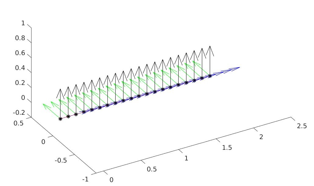
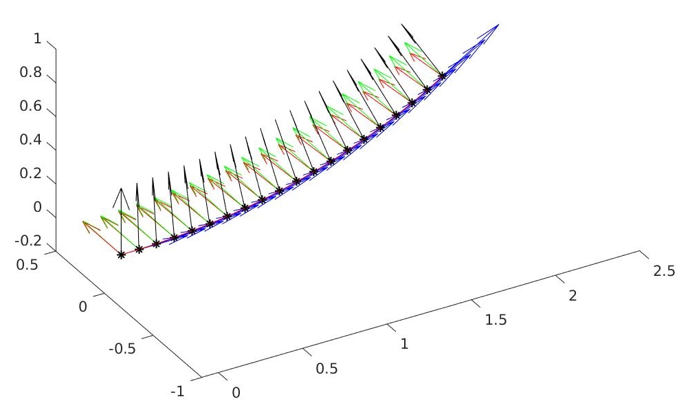
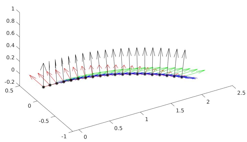
Figure 1: Deformation of the rod in Example 3.1. From left to right we have $t=0$, $t=30$ and $t=40$. The different coloured arrows represent the vectors $y^{\prime}$, $b$ and $d=y^{\prime}\wedge b$, that form the frame $R$, as well as the LCE-director $n=R\hat{n}$. The two rightmost graphics show, that the LCE-director $n$ tends to align with the vectors $f_{\operatorname{odd}}=(0,1,0)$ or $f_{\operatorname{even}}=(1,0,0)$ at the end of the intervals $I_{3}$ and $I_{4}$ respectively.

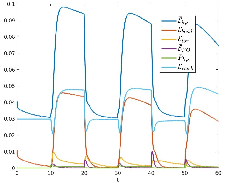
Figure 2: Energy development over the (quasi-) time interval in Example 3.1. The different curves represent the energy term $\bar{\mathcal{E}}_{h,\varepsilon}$, the bending energy, the torsion energy, the Frank-Oseen energy, the penalty term $P_{h,\varepsilon}$ and the contribution of $\bar{\mathcal{E}}_{\operatorname{res},h}$. The energy is non-decreasing in some parts. This is due to the fact that the energy functional $\bar{\mathcal{E}}_{h,\varepsilon}$ does not include the forcing term $-\left(f,R\hat{n}\right)_{L^{2}(\omega)}$, which was added to simulate a magnetic field, and it takes some time until $n$ and $f$ are realigned after $f$ changes.

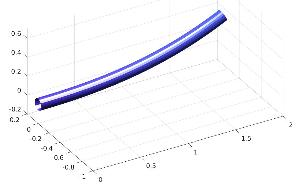
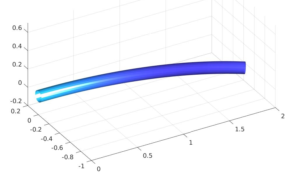
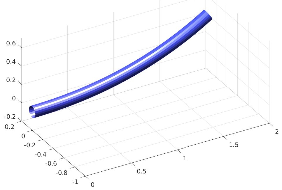
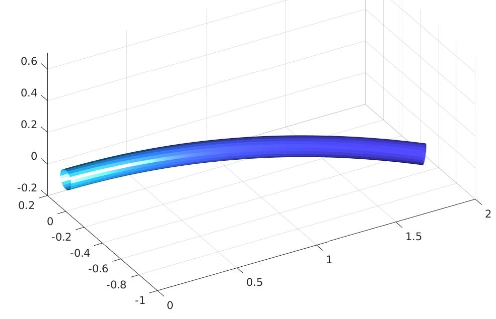
Figure 3: Deformation of the rod from Example 3.1. The top row shows the configurations at $t=10$ and $t=20$, while the bottom row shows $t=30$ and $t=40$. The colouring of the tube represents its curvature.

In the Figures 2 and 3 we can see the development of energy and deformation within $(0,T)$. For both values of $f$ we observe a different deformation the rod seems to converge to, basically enabling us to switch between two states. However, the deformations and energy at the end of the different time intervals corresponding to the same value of $f$ are slightly different. This can be explained by the fact, that these intervals are too short for a full relaxation and convergence to the minimizer. Indeed we observe smaller differences when using longer time intervals.

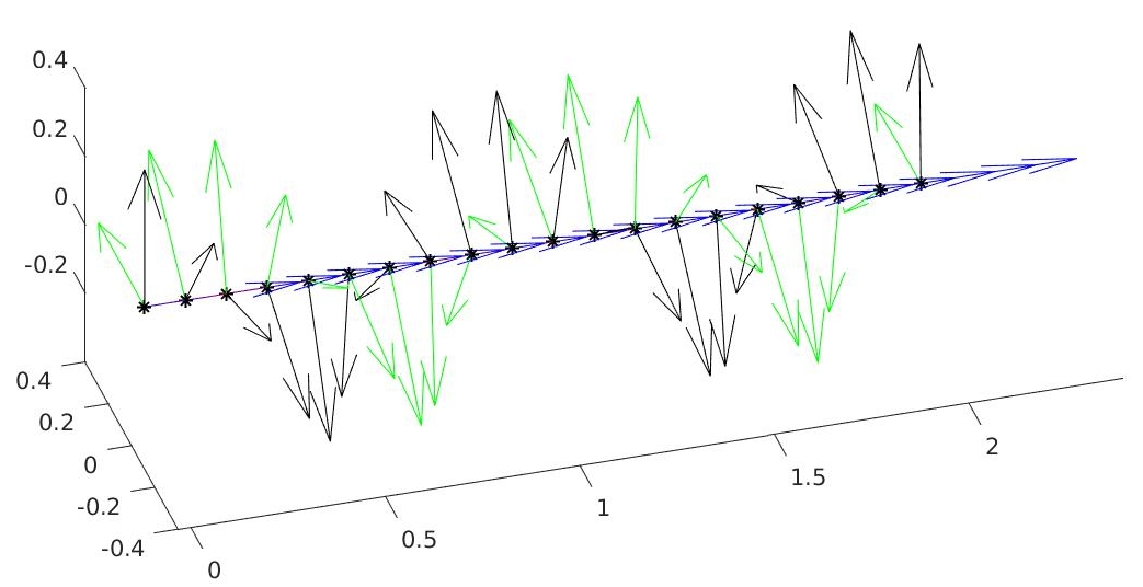
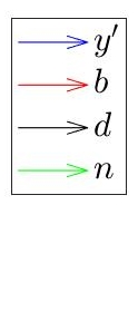
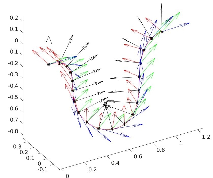
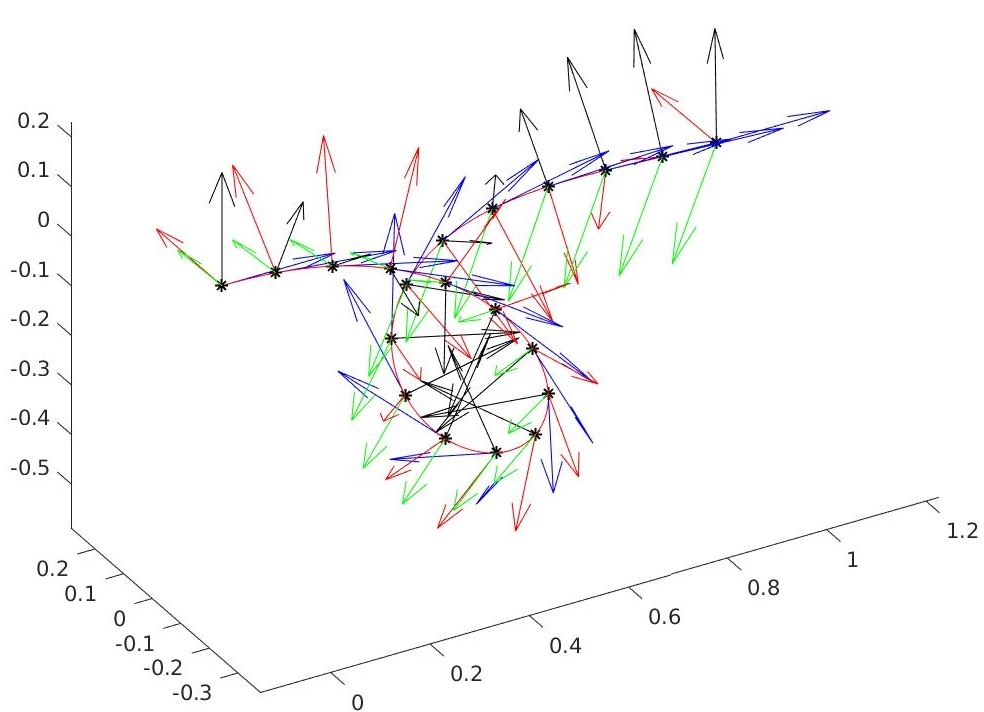
Figure 4: Buckling behaviour of the rod from Example LABEL:ex_buckling. The top row shows the starting configuration while the bottom row depicts the relaxed state at time $t=50$ with $\bar{r}=1$ (left) and $\bar{r}=3$ (right). As in Figure 1, the vectors $y^{\prime}$, $b$ and $d=y^{\prime}\wedge b$, that form the frame $R$, as well as the LCE-director $n=R\hat{n}$ are shown.