Scalable Multi-Agent Model-Based Reinforcement Learning

Abstract.

Recent Multi-Agent Reinforcement Learning (MARL) literature has been largely focused on Centralized Training with Decentralized Execution (CTDE) paradigm. CTDE has been a dominant approach for both cooperative and mixed environments due to its capability to efficiently train decentralized policies. While in mixed environments full autonomy of the agents can be a desirable outcome, cooperative environments allow agents to share information to facilitate coordination. Approaches that leverage this technique are usually referred as communication methods, as full autonomy of agents is compromised for better performance. Although communication approaches have shown impressive results, they do not fully leverage this additional information during training phase. In this paper, we propose a new method called MAMBA which utilizes Model-Based Reinforcement Learning (MBRL) to further leverage centralized training in cooperative environments. We argue that communication between agents is enough to sustain a world model for each agent during execution phase while imaginary rollouts can be used for training, removing the necessity to interact with the environment. These properties yield sample efficient algorithm that can scale gracefully with the number of agents. We empirically confirm that MAMBA achieves good performance while reducing the number of interactions with the environment up to an orders of magnitude compared to Model-Free state-of-the-art approaches in challenging domains of SMAC and Flatland.

1. Introduction

Reinforcement Learning (RL) has achieved numerous breakthroughs Berner et al. (2019); Vinyals et al. (2019); Silver et al. (2016) in recent years both for single- and multi-agent environments. However, sample efficiency has always been a prominent issue as a tremendous number of interactions is required by Model-Free Reinforcement Learning (MFRL) approaches to achieve optimal performance. Model-Based Reinforcement Learning (MBRL) tries to alleviate this issue by allowing the agent to interact with a learned model of the environment instead. It has shown success both in environments with known world dynamics such as shogi or go Schrittwieser et al. (2020) and where dynamics need to be learned from samples such as Atari Kaiser et al. (2019); Hafner et al. (2020). However, translating this success to multi-agent settings is non-trivial. Several studies Krupnik et al. (2020); Schwarting et al. (2021) have shown that MBRL approaches can be much more sample efficient than their MFRL counterparts in environments with two agents. Nonetheless, all of the current state-of-the-art MFRL approaches on popular multi-agent benchmarks such as StarCraft Multi-Agent Challenge Samvelyan et al. (2019) remain uncontested.

One of the major paradigms in Multi-Agent Reinforcement Learning is Centralized Training with Decentralized Execution (CTDE) Foerster et al. (2018); Rashid et al. (2018); Lowe et al. (2017), which holds to the premise that we can use additional information during training as long as execution remains decentralized. This paradigm is well-motivated when we want full autonomy for the agents Maes (1993), for example, when the task is not fully cooperative because agents might not want to share their information with others Cao et al. (2018); Blumenkamp and Prorok (2020); Noukhovitch et al. (2021). Furthermore, in many real world scenarios, such as autonomous driving Desjardins and Chaib-Draa (2011) or drone management Azar et al. (2021), agents must collaborate with each other to achieve their goals and they can also share information for better coordination. This setup is usually defined as a communication technique Foerster et al. (2016); Liu et al. (2020), as the agents no longer have full autonomy yet they can leverage the messages from others to make their decisions. As a part of CTDE, communication methods usually restrict the message channel either by limiting bandwidth or receiving messages only from the neighbours in the environment Gronauer and Diepold (2021). Other CTDE techniques can still be applied together with the communication technique to stabilize learning or solve the credit assignment issue. Note that if we decide to centralize execution even more, reducing the multi-agent problem to single-agent, this solution will suffer from scalability issues as the number of states and actions will grow exponentially with the number of agents. Thus, communication methods strike a balance between autonomy of the agents and efficiently using available information to make decisions in collaborative environments. However, previous studies do not fully leverage this additional shared information during the training phase.

In this paper, we show that communication can be sufficient to sustain a world model, making it possible to exploit centralized training further by training policies without interacting with the environment. Furthermore, it is sufficient to only communicate discrete messages with the neighbouring agents to update a world model during execution phase. We denote our approach as MAMBA, which is derived from Multi-Agent Model-Based Approach. To our knowledge, this is the first method that extends world models to environments with an arbitrary number of agents and that views world models as an instance of communication. We show that our method can reduce the required number of samples by an order of magnitude compared to MFRL approaches and consistently outperform current state-of-the-art methods in low data regime in challenging environments of SMAC Samvelyan et al. (2019) and Flatland Mohanty et al. (2020).

2. Definitions and Background

2.1. Markov Game

A Markov game Littman (1994) is a tuple $\mathcal{G}=(S,n,\mathcal{A},O,T,r)$, where $S$ is a set of states $s$, $n$ is a number of players, $\mathcal{A}_{i}$ is a set of actions $a$ of player $i$. $\mathcal{O}:S\times N\rightarrow\mathbb{R}^{d}$ is an observation function that specifies d-dimensional observations available to each agent and $O_{i}$ is set of observations $o_{i}$ of agent $i$. $T:S\times\mathcal{A}_{1}\times\dots\times\mathcal{A}_{n}\rightarrow\Delta(S)$ and $r_{i}:S\times\mathcal{A}_{1}\times\dots\times\mathcal{A}_{n}\rightarrow\mathbb{R}$ are transition and reward functions respectively, where $\Delta$ is a discrete probability distribution over $S$. We define $\Delta_{0}(S)$ as the distribution of initial states and return of player $i$ in state $s$ with discount factor $\gamma\in[0,1)$ as $R_{i}(s)=\overset{\infty}{\underset{t=0}{\sum}}\left[\gamma^{t}r_{i}(s_{t},a^{1}_{t},\dots,a^{n}_{t})\mid s_{0}=s\right]$. Each player has its own policy $\pi_{i}:O_{i}\rightarrow\Delta(\mathcal{A}_{i})$ that returns probability for each action to be taken when observing $o_{i}$ and value function $V_{i}(s)=\mathop{\mathbb{E}}_{\pi_{i}}[R_{i}(s)]$. We also define Q-function as $Q_{i}(s,a)=\mathop{\mathbb{E}}_{\pi_{i}}[R_{i}(s)\mid a^{i}_{0}=a]$. Bold font will denote vector, e.g. $\textbf{a}=(a^{1},\dots,a^{N})$ and subscript $a_{t}$ will denote current step in the environment.

2.2. Single-Agent Reinforcement Learning

Model-Free Reinforcement Learning.

There are two major MFRL frameworks, namely Q-learning Watkins and Dayan (1992) and Actor-Critic Mnih et al. (2016). In Actor-Critic framework, the Actor’s goal is to learn a policy $\pi(s)$ that maximizes agents returns predicted by the Critic. A widely-used method is proximal policy optimization (PPO) Schulman et al. (2017), where the Actor’s neural network is trained on the following loss:

$$\mathcal{L}_{\pi}(A_{t})=-\min(\mathcal{R}_{t}A_{t},clip(\mathcal{R}_{t},1-\epsilon,1+\epsilon)A_{t})$$ (1)

where $\mathcal{R}_{t}=\frac{\pi(s_{t})}{\pi_{old}(s_{t})}$ denotes probability ratio of the policies after and before the update and $A_{t}$ is an advantage function predicted by the Critic. Using this loss ensures that the agent’s policy makes a conservative update within a trust region. The advantage is defined as $A_{t}=y_{t}-V_{t}$, where $y_{t}=r_{t}+\gamma V_{t+1}$. The Critic’s neural network is independently trained to predict $V_{t}$ by minimizing squared TD error $(y_{t}-V_{t})^{2}$. In Q-learning framework, we do not have a policy $\pi(s)$ and instead use learned Q-function directly to predict next action.

Model-Based Reinforcement Learning.

MBRL approaches Sutton (1991) additionally learn a world model that includes both transition function $T$ and reward function $r$. Decoupling learning dynamics of the system from the decision making allows us to use more sophisticated unsupervised learning techniques to represent current state in latent space as well as to use imaginary rollouts for training Kaiser et al. (2019); Hafner et al. (2020). Many previous works provide both theoretical and empirical evidence that MBRL approaches can be much more sample efficient than their MFRL counterparts. Recent breakthroughs of Dreamer Hafner et al. (2019a, 2020) also showed that MBRL is capable of achieving same or better performance than Model-Free approaches both in continuous and discrete environments.

2.3. Multi-Agent Reinforcement Learning

In Multi-Agent Reinforcement Learning (MARL), multiple agents learn and interact in the same environment. In this paper, we will focus on cooperative environments Samvelyan et al. (2019), where agents have the same goal and they need to collaborate with each other to achieve it. One naive approach in MARL is training agents independently using unmodified single-agent RL techniques Tan (1993); de Witt et al. (2020). However, it does not have any convergence guaranties due to the inherent non-stationarity of multi-agent environments resulting from the constantly changing policies of other agents Laurent et al. (2011); Hernandez-Leal et al. (2017). On the other side of the spectrum, we could look at the multi-agent problem as a single-agent one. This yields a fully centralized approach that controls all agents simultaneously based on global information. Consequently, a centralized solution cannot scale to a large number of agents due to the resultant exponential growth of the action space, known as the familiar ’curse of dimensionality’ Sunehag et al. (2017). This leaves us with one viable technique to train agents in multi-agent environments, namely Centralized Training with Decentralized Execution. We also explicitly highlight the communication technique, which is considered part of CTDE Gronauer and Diepold (2021), that allows an additional message channel during execution for better coordination.

Centralized Training with Decentralized Execution

CTDE is a combination of independent and centralized MARL Kraemer and Banerjee (2016); Lowe et al. (2017); Sunehag et al. (2017); Rashid et al. (2018); Foerster et al. (2018); Son et al. (2019). This paradigm allows additional information to be used in training provided that execution is still decentralized. This enhancement can help to alleviate the issues of credit assignment and non-stationarity as we no longer need to rely only on local observations and rewards during training. Decentralized execution also ensures that we deal with the curse of dimensionality as agents still make their decisions independently based on relevant local information.

Communication can be seen as a part of the CTDE paradigm as we can still use additional information on the training stage, but now we allow agents to communicate with each other during execution, which is a natural assumption for cooperative environments Liu et al. (2020); Sukhbaatar et al. (2016); Foerster et al. (2016) where agents have the same goal and can also be used in mixed environments Singh et al. (2018) to promote cooperation. Despite being considered CTDE Gronauer and Diepold (2021), we argue that communication can greatly benefit from possessing certain properties to ensure decentralized execution. In this paper, we will focus on the two desirable properties of communication that can greatly improve scalability and decentralization of the agents. The first property is called discrete communication and is strongly connected with the limitation of the message channel bandwidth as it restricts agents to sending each other only discrete messages Gronauer and Diepold (2021); Foerster et al. (2016). This property allows us to significantly reduce the number of bits for message transmission and can be considered a universal restriction between the environments on the number of bits allowed for one message. The second property is called locality Zhang et al. (2018), which can be naturally defined in most environments. This property allows an agent to communicate only with its neighbours on the map, which makes the decision making decentralized since each agent takes action individually based only on local information Zhang et al. (2018). Unfortunately, some environments do not exhibit this locality property either because the map is too small or coordination between all agents is required to solve the task.

Multi-Agent Deep Deterministic Policy Gradient (MADDPG)

Lowe et al. (2017) MADDPG is a CTDE algorithm specifically designed for mixed environments. MADDPG shows that augmenting critics with the states and actions of all agents can reduce the variance of policy gradients, which can improve performance.

Counterfactual Multi-Agent policy gradients (COMA)

Foerster et al. (2018) COMA is an Actor-Critic algorithm designed to alleviate the credit assignment issue in multi-agent environments. The core idea is based on Difference Rewards Wolpert and Tumer (2002), which compares the current global reward of the agent to the average reward that the agent can get in the current state. COMA applies this idea to Q-functions of agents, additionally using augmented critics similar to MADDPG.

QMIX

Rashid et al. (2018) QMIX is an algorithm designed for training Q-learning agents in cooperative environments. As with COMA, it tries to solve credit assignment using additional information during training. As agents still need the Q-function during execution, we cannot alter its input as in COMA. QMIX proposes to use a mixer function to combine Q-functions of agents into a centralized Q-function that is trained on global reward. QMIX ascertains that mixer function ensures monotonicity in its inputs, which makes the argmax of the agents’ Q-functions consistent with the argmax of the centralized Q-function. This property is called Individual-Global-Max (IGM) and is essential for factorizing the global Q-function to agents’ Q-Functions.

QTRAN

Son et al. (2019) QTRAN is an algorithm that extends the class of functions that we can factorize compared to QMIX. QTRAN shows that the monotonicity property can be lifted from the mixer function and introduces additional ”track” losses that keep the agents’ Q-functions close to the global Q-function, which is sufficient to preserve the IGM property but introduces additional training complexity.

CommNet

Sukhbaatar et al. (2016) CommNet is a communication algorithm that employs continuous protocols. CommNet uses LSTM Hochreiter and Schmidhuber (1997) to process messages and shows that communication can be essential in solving tasks in partially observable environments.

G2A

Liu et al. (2020) G2A is an algorithm that uses two-stage attention architecture to process messages from other agents. The first stage uses Hard Attention to detect relevant agents in the environment, while the second stage uses Soft Attention to process messages from these agents.

2.4. Attention Mechanism

Attention Vaswani et al. (2017); Bahdanau et al. (2014) has become an ubiquitous approach for sequence data processing, achieving state-of-the-art performance in multitude of fields such as NLP Devlin et al. (2018) and CV Dosovitskiy et al. (2020). It has also shown to be useful in MARL when processing input observations of all agents Vinyals et al. (2019) or solving credit assignment Iqbal and Sha (2019).

In this paper, we will focus mainly on self-attention, which takes as an input value matrix $V$ with dimensionality $n\times d$ and for each of $n$ vectors outputs weighted average of the whole vector sequence. There are two types of attention mechanism, namely soft attention and hard attention Shen et al. (2018). Following Vaswani et al. (2017), the former assigns the weights for each value vector using this formula:

$$\text{Soft Self-Attention}(Q,K,V)=\text{softmax}(\frac{QK^{T}}{\sqrt{d}})V$$ (2)

where $Q$, $K$, $V$ are linear projections of the value vectors, and latter assigns either zeroes or ones depending on the relevance of the vector.

3. MAMBA

In this section, we describe our method called Multi-Agent Model-Based Approach (MAMBA). First, we formulate the desiderata for the method and review existing papers that tackle the outlined problems. Second, we describe our method and its communication properties.

3.1. Desiderata

Sample Efficiency

One of the main strengths of MBRL approaches is the sample efficiency that results from using imaginary rollouts provided by the learned model. In the single-agent setting, multiple papers provide empirical evidence Kaiser et al. (2019); Hafner et al. (2019a, 2020) as well as theoretical justifications Agarwal et al. (2020); Azar et al. (2013); Li et al. (2020) that MBRL approaches achieve near-optimal sample efficiency compared to Model Free approaches. This theory is further extended to the multi-agent setting Liu et al. (2021); Zhang et al. (2020). However, empirical performance is still lacking due to the increased complexity of the model and exponential growth of the action and state spaces.

Addressing non-stationarity

Experience replay buffer is a popular technique for off-policy learning that has been shown to improve sample efficiency compared to on-policy algorithms Andrychowicz et al. (2017). However, in multi-agent environments collected experience quickly becomes irrelevant due to the inherent non-stationarity Hernandez-Leal et al. (2017). Methods have been proposed by Foerster et al. (2017) to alleviate non-stationarity using techniques such as importance sampling and fingerprinting. However, these techniques can suffer from large variance as the agents progressively change their policies Precup (2000). Another approach is to use on-policy algorithms and a world model that approximates the environment’s dynamics, which can be used to roll out imaginary trajectories starting from the states in the buffer for current policies, thus mitigating any issues with irrelevant experience Zhang et al. (2020).

Scalability

One of the key problems of learning dynamics of multi-agent environments is the curse of dimensionality. We want the world model to scale to a large number of agents in the environment, which would require the model to manage the resultant exponential growth of state and action spaces. This would allow it to process large numbers of transitions during both training and inference phases.

Locality

Multiple studies Wang et al. (2020b); Liu et al. (2020) have shown that in large environments it is possible to significantly reduce the state space to comprise only relevant information for the agents’ decision making. This reduction can be naturally applied to environments like autonomous driving Singh et al. (2018), where an agent only needs to be informed about cars in its local view. This property of locality can also be applied to communication Liu et al. (2020); Zhang et al. (2018) by the same reasoning. Ideally, a world model should have a locality property, so that if the environment allows us to define neighbours of the agent, we want to communicate only with them during execution.

Discrete Communication

One dichotomy between the communication protocols is that the message can be either continuous Sukhbaatar et al. (2016) or discrete Foerster et al. (2016). It is desirable that agents communicate using discrete messages, as it is more suitable for channels with limited bandwidth. Discrete representation allows us to greatly reduce the amount of information broadcast by the agents, which can be essential for deploying communication methods in the real world. Note that even with a restricted message channel, discrete messages can greatly enhance the performance of the agents Foerster et al. (2016).

Decentralized Execution

Finally, we want to deploy agents in a decentralized fashion, so they can make their decisions independently based on their local observations and messages from other agents Zhang et al. (2018). To this end, one of the main paradigms is CTDE Rashid et al. (2018); Foerster et al. (2018); Liu et al. (2020); Sukhbaatar et al. (2016), which achieves strong performance in multi-agent domains while maintaining decentralization on the execution stage. We want to learn a world model that can be sustained in a decentralized manner during execution using only communication between agents.

3.2. Architecture

Figure 1. Training Phase. Transitions $(o^{i}_{t-1},a^{i}_{t-1},o^{i}_{t})$ are sampled from the buffer. Agents use the Communication Block to predict their current state feature vectors $e^{i}_{t}$ from stochastic states and actions from previous step $(z^{i}_{t-1},a^{i}_{t-1})$. These feature vectors are then used to update the hidden state of the model $h^{i}_{t}$. Agent then can predict current stochastic state $z^{i}_{t}$ from $h^{i}_{t}$ and its current observation $o^{i}_{t}$ and in turn use it to predict local information such as observation $\hat{o}^{i}_{t}$ and reward $\hat{r}^{i}_{t}$. Agent also uses stochastic state to predict its next action $a^{i}_{t}$. During the imaginary rollout stage, Communication Block utilizes predicted stochastic states $\hat{z}^{i}_{t}$ instead of $z^{i}_{t}$ and observations $o^{i}_{t}$ are not used.

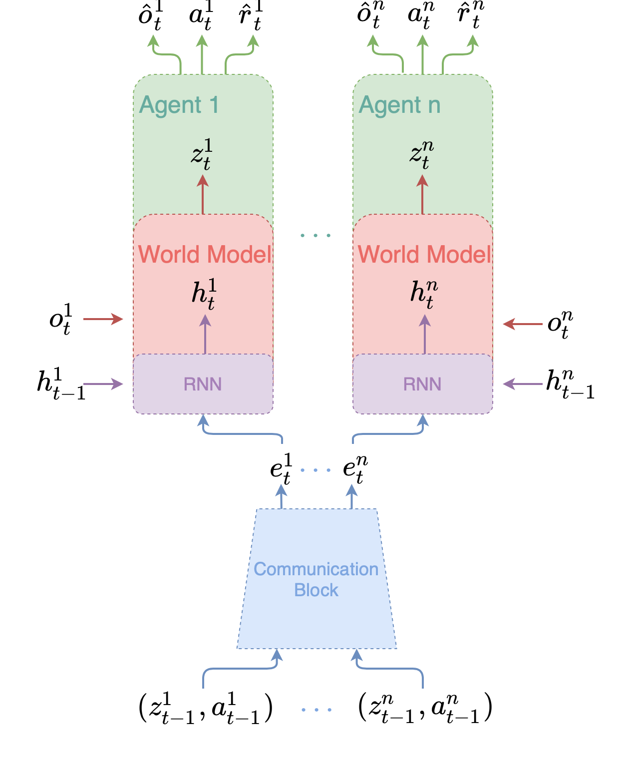
We chose DreamerV2 Hafner et al. (2020), a state-of-the-art MBRL approach for discrete environments, as a backbone for our algorithm. Following Dreamer notation, the model consists of six components:

$$\text{RSSM}=\left\{\begin{array}[]{ll}\text{Recurrent model:}&h^{i}_{t}=f_{\phi}(h^{i}_{t-1},\textbf{z}_{t-1},\textbf{a}_{t-1})\\[2.0pt] \text{Representation model:}&z^{i}_{t}\sim q_{\phi}(z^{i}_{t}\mid h^{i}_{t},o^{i}_{t})\\[2.0pt] \text{Transition predictor:}&\hat{z}^{i}_{t}\sim p_{\phi}(\hat{z}^{i}_{t}\mid h^{i}_{t})\end{array}\right.$$

$$\begin{array}[]{ll}\hskip 38.41139pt\text{Observation predictor:}&\hat{o}^{i}_{t}\sim p_{\phi}(\hat{o}^{i}_{t}\mid h^{i}_{t},z^{i}_{t})\\[2.0pt] \hskip 38.41139pt\text{Reward predictor:}&\hat{r}^{i}_{t}\sim p_{\phi}(\hat{r}^{i}_{t}\mid h^{i}_{t},z^{i}_{t})\\[2.0pt] \hskip 38.41139pt\text{Discount predictor:}&\hat{\gamma}^{i}_{t}\sim p_{\phi}(\hat{\gamma}^{i}_{t}\mid h^{i}_{t},z^{i}_{t})\end{array}$$

where the RSSM model Hafner et al. (2019b) is used to learn the dynamics of the environment and Observation, Reward and Discount predictors are used for reconstructing corresponding variables. We learn Observation, Reward and Discount predictors similar to Hafner et al. (2020) via supervised loss and Representation model by minimizing the evidence lower bound Kingma and Welling (2013). Transition predictor is then trained by minimizing KL divergence between $\hat{z}^{i}_{t}$ and $z^{i}_{t}$, where $z^{i}_{t}$ is a stochastic state sampled from categorical distribution same as in DreamerV2. Recurrent model consists of 1 layer GRU Cho et al. (2014) as in the original DreamerV2 implementation. In order to facilitate independence between hidden states $\textbf{h}_{t}$, we predict individual reward, discount and observation only from agent’s latent state. We also use the sum of KL divergences between individual stochastic states $\hat{z}^{i}_{t}$ by applying the chain rule to the true Transition function:

$$p_{\phi}(\hat{\textbf{z}}_{t}\mid\textbf{h}_{t})=p_{\phi}(\hat{z}^{1}_{t}\mid\textbf{h}_{t})\cdots p_{\phi}(\hat{z}^{n}_{t}\mid\textbf{h}_{t},\hat{z}^{1}_{t},\ldots,\hat{z}^{n-1}_{t})$$ (3)

However, predicting latent states autoregressively is too impractical and we elaborate on its substitute in the next paragraph. The final loss for learning the world model consists of:

$$\begin{array}[]{ll}\text{Observation loss:}&-\ln{p_{\phi}(o^{i}_{t}\mid h^{i}_{t},z^{i}_{t})}\\[2.0pt] \text{Reward loss:}&-\ln{p_{\phi}(\hat{r}^{i}_{t}\mid h^{i}_{t},z^{i}_{t})}\\[2.0pt] \text{Discount loss:}&-\ln{p_{\phi}(\hat{\gamma}^{i}_{t}\mid h^{i}_{t},z^{i}_{t})}\\[2.0pt] \text{KL divergence loss:}&\text{KL}\left[q_{\phi}(z^{i}_{t}\mid h^{i}_{t},o^{i}_{t})\lVert p_{\phi}(\hat{z}^{i}_{t}\mid h^{i}_{t})\right]\\ \end{array}$$

which is calculated in expectation over $q_{\phi}(\textbf{z}_{1:T}\mid\textbf{a}_{1:T},\textbf{o}_{1:T})$ and summed over all $n$ agents and rollout length $T$. As in Dreamer, all losses are optimized jointly using the Adam optimizer Kingma and Ba (2014). Note that we do not use an additional $\beta$ weight for KL divergence Higgins et al. (2016) to simplify algorithm complexity. As in DreamerV2, we use KL balancing to facilitate learning of prior $p_{\phi}(\hat{z}^{i}_{t}\mid h^{i}_{t})$ by assigning a larger weight to cross entropy and a lower weight to posterior entropy in the KL term. The schematic representation of the training phase is in Figure 1.

Transition function.

In our method, we implement Transition function using Attention. Simply predicting next latent states independently using Attention can create inconsistencies between agents’ current views of the environment, which can hinder performance. To solve this issue, we could theoretically predict next latent states autoregressively, that is, condition the latent state of $i$-th agent on the predicted latent states of the previous agents. However, this would significantly slow down training and would not allow decentralized decision making during execution. Another approach, proposed by Krupnik et al. (2020), is to maximize mutual information between the latent state and the previous action of the agent:

$$\mathcal{L}_{\text{info}}=-I((h^{i}_{t},z^{i}_{t});a^{i}_{t-1})$$ (4)

This way, we encourage the latent state to depend mostly on its own actions, thus making it less dependent on others. Consequently, this disentanglement of the agent’s latent space allows us to dispatch them separately. We use the lower bound proposed by Chen et al. (2016) to practically maximize mutual information by training an additional neural network to predict previous action from the latent state of the agent:

$$\mathcal{L}_{\text{info}}=-\ln{p_{\phi}(a^{i}_{t-1}\mid h^{i}_{t},z^{i}_{t})}$$ (5)

Stochastic state

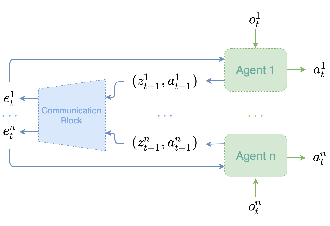
During the execution and imaginary rollout stages, agents are allowed to transmit only their stochastic states $z^{i}_{t}$. As in DreamerV2, stochastic state has a discrete nature and consists of $32$ categorical distributions with $32$ classes each. Straight-through gradients Bengio et al. (2013) are used to learn these discrete representations. By design, stochastic state is the only message that can be broadcasted by the agent, which amounts only to $32\log{32}=160$ bits of information per message. This is largely because of the sparsity of the $z^{i}_{t}$ compared to the other possible distributions. We can also use a language-based interpretation Foerster et al. (2016); Lazaridou et al. (2016) of $z^{i}_{t}$ as we restrict agents to a very limited vocabulary to express their current states. We further elaborate on this point in the next section.

Communication Block

We use Transformer architecture Vaswani et al. (2017) with 3 stacked layers for encoding state-action pairs $(\textbf{z}_{t},\textbf{a}_{t})$. These encodings $e^{i}_{t}$ are then used by the agents to update the world model and make action predictions. We use a dropout technique Srivastava et al. (2014) with probability $p=0.1$ to prevent the model from overfitting and use positional encoding Vaswani et al. (2017) to distinguish agents in homogeneous settings.

Absorbing states.

One major difference between single- and multi-agent environment dynamics is the varying number of agents on the map. Even if the starting number of agents is always the same, it is natural that agents will have varying trajectory lengths depending on the task. Thus, it is essential to handle the states of the agents that are no longer present in the environment during the training phase. Absorbing state Kostrikov et al. (2018) is an imaginary state that does not yield a reward for any action and does not lead to any other state, creating an infinite loop to itself. In our implementation, we add absorbing states after the end of an agents trajectory, so that it does not get a reward for future actions and so other agents can see that that agent is no longer on the map. We do not use observation loss to learn the representation of those states as no meaningful observation can be provided by the environment. Instead, we allow the world model to implicitly learn those representations only from predicting the discounts and rewards that are both equal to zero.

Behaviour learning. We chose Actor-Critic framework to learn an agent’s behaviour, where both actor and critic are parameterized by neural networks $\psi$ and $\eta$ respectively:

$$\begin{array}[]{ll}\text{Actor:}&a^{i}_{t}\sim p_{\psi}(a^{i}_{t}\mid\hat{z}^{i}_{t},h^{i}_{t})\\ \text{Critic:}&v_{\eta}^{i}(\hat{\textbf{z}}_{t})\approx\mathop{\mathbb{E}}_{p_{\psi}}\left[\overset{\infty}{\underset{\tau=t}{\sum}}\gamma^{i}_{\tau}r^{i}_{\tau}\right]\\ \end{array}$$

Imaginary rollouts

As in Dreamer, we use learned transition function $p_{\phi}(\hat{z}^{i}_{t}\mid h^{i}_{t})$ to predict the next stochastic state based on agents’ actions and current states of the model. Starting from initial states sampled from the replay buffer, we generate rollouts based on current policies of the agents in order to deploy on-policy learning algorithms in the latent space. We set the length of the imaginary rollouts to $H=15$ to account for increased complexity of the multi-agent environments and possible compounding error Janner et al. (2019) of the world model.

Figure 2. Execution Phase. Each agent has its own version of the world model, which can be updated using the Communication Block. It is sufficient to send only stochastic state $z^{i}_{t-1}$ and action $a^{i}_{t-1}$ from the previous step for each agent in order to obtain feature vectors $e^{i}_{t}$. Agent $i$ then can use the updated world model and its current observation $o^{i}_{t}$ to output its next action $a^{i}_{t}$.

(a) Flatland

(b) StarCraft Multi-Agent Challenge

Figure 3. Environments

Actor

Instead of using Reinforce Williams (1992) for policy updates as in Dreamer, we found that for multi-agent environments PPO updates (Eq. 1) yield better results. We do not use gradients backpropagated through the dynamics model as they hinder the performance, which is likely due to its high noisiness in multi-agent environments. We use parameter sharing Gupta et al. (2017) for the actor network to accelerate training.

Critic

We use $\lambda$-target Schulman et al. (2015) for value function as in Dreamer, which gives us more unbiased estimates than TD-error Sutton and Barto (2018). We augment critic by giving it as an input all current latent states $\hat{\textbf{z}}_{t}$, which are processed using Attention mechanism. Unlike other CTDE approaches Lowe et al. (2017); Rashid et al. (2018), we cannot use additional information beyond the states predicted by the model as we train agents in the latent space. However, several studies de Witt et al. (2020); Wang et al. (2020a) suggested that such additional information can cause centralized-decentralized mismatch, which can hinder the learning process due to the large variance of the policy gradient updates. Furthermore, in real world scenarios we would not have such additional information as the global environment may be too large.

3.3. Communication

Here, we discuss the properties of our communication protocol. Similar to methods employing Attention mechanism to collect useful information from other agents Liu et al. (2020); Das et al. (2019); Jiang and Lu (2018), we allow agents to broadcast their latent state representations from the previous step $\textbf{z}_{t-1}$. We also assume that agents can observe actions $\textbf{a}_{t-1}$ of others. Tuples $(\textbf{z}_{t-1},\textbf{a}_{t-1})$ are then transformed by Communication Block to feature vector $e^{i}_{t}$ that is used to update the agent’s world model and predict next action based on the updated latent state. The schematic representation of the execution phase is in Figure 2.

Reward-agnostic communication

One important distinction of MAMBA communication from other communication protocols Sukhbaatar et al. (2016); Foerster et al. (2016); Das et al. (2019) is that it is not learned from the reward signal. We will refer to our communication protocol as reward-agnostic communication as we use a world model to obtain it, and we will denote communication protocols from Sukhbaatar et al. (2016); Foerster et al. (2016); Das et al. (2019) as goal-oriented communication as they are shaped by the agent’s reward. We argue that reward-agnostic communication is more suited for language that describes current environment while goal-oriented communication is more suited for describing agent’s task. This duality is mirrored in language theory as representation and acquisition theories respectively Ellis and Larsen-Freeman (2006). We can think of reward-agnostic communication as an emergent language that agents cannot alter to their needs but in exchange this language can provide an unbiased representation of the current state of the agent. On the other hand, goal-oriented communication is defined by the needs of the agent, thus making it a useful tool to achieve its goals. Consequently, many previous works on communication Cao et al. (2018); Blumenkamp and Prorok (2020); Noukhovitch et al. (2021) studied this phenomenon as selfish agents tried to manipulate the communication channel to their own advantage by sending false messages to others. Conversely, we cannot use reward-agnostic communication in mixed environments as it provides true information about the agent to both allies and competitors.

Locality

As we want to preserve locality as much as possible, we can make the agent receive messages only from its neighbours in the environment. Attention mechanism allows us to vary the number of messages and, assuming that agents which are not neighbours will not have an impact on the agent transition function, it is possible to mask weights of those agents in Attention.

Discrete communication

Multiple studies have shown that discrete messages enhance performance as agents develop the language to communicate with each other Havrylov and Titov (2017); Lazaridou et al. (2016); Foerster et al. (2016). On the other hand, language capabilities to succinctly describe images in only a few words have inspired several studies in representation learning Oord et al. (2017); Razavi et al. (2019) to use discrete stochastic states. In our communication protocol, we can see the duality of these ideas as we can train stochastic states on unsupervised loss to reason about the current state of the agent and at the same time use it to communicate agent’s current surroundings.

Computation-Communication trade-off

Broadcasting only tuples $(\textbf{z}_{t-1},\textbf{a}_{t-1})$ to all agents requires $\mathcal{O}(n^{2})$ computations on each agent to calculate single-layer attention encodings Vaswani et al. (2017). Alternatively, agents can compute only one vector from $n$, for example, $q^{i}K^{T}$ from Eq. 2, and exchange computed vectors on each step of attention to reduce computation complexity to $\mathcal{O}(n)$.

3.4. Limitations and Improvements

MAMBA satisfies all of the stated desiderata by leveraging a Model-Based approach for large scale multi-agent environments. However, MBRL has several limitations compared to MFRL methods. First, learning the world model introduces additional complexity to the Reinforcement Learning algorithm, which requires more careful tuning of hyperparameters. Second, while MAMBA is able to achieve good performance in most environments in a low data regime, it also requires more computational time for one collected trajectory compared to MFRL methods as it needs to learn the world model and rollout imaginary trajectories to learn the policy. We provide detailed comparisons of average wall clock time for training and execution with the same hardware in Appendix.

4. Experiments

(a) 2s vs 1sc

(b) so many baneling

(c) 3s vs 3z

(d) 3s vs 4z

(e) 8m vs 9m

(f) 25m

(g) corridor

(h) 3s5z vs 3s6z

Figure 4. Experiments in SMAC environments. Y axis denotes winning rate of the agents and X axis denotes number of steps taken in the environment.

4.1. Environments

Flatland

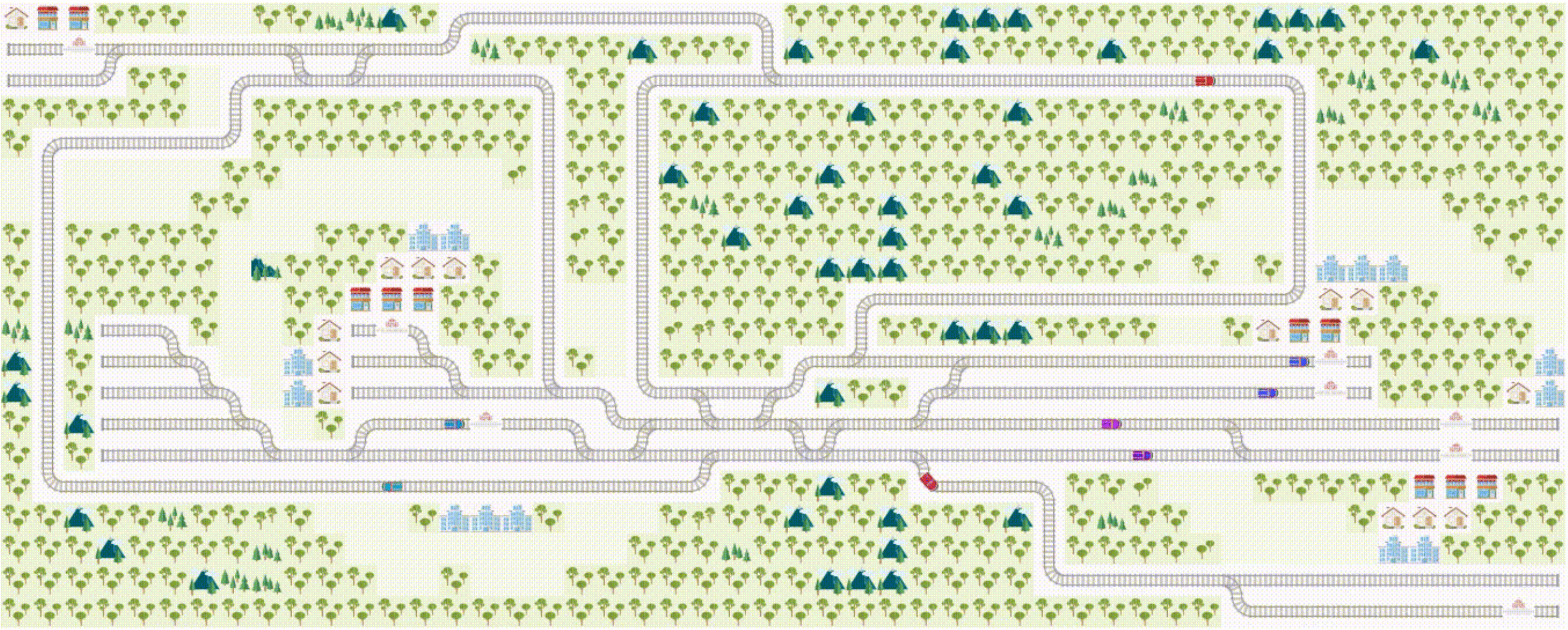
Mohanty et al. (2020) (Figure 3a) is a multi-agent 2d environment simulating train traffic on the rail network. Each agent has its own starting point and destination and the goal of the environment is to guide agents to their destinations without collisions. The difficulty of the environment can be flexibly adjusted as the number of agents as well as the size of the map could be easily configured. Note that maps are generated procedurally for each trajectory, so the world model must be able to generalize well in order to achieve good performance. Each agent receives positive reward on arrival to its destination and negative reward if a collision occurs. We additionally use more dense variant of the reward provided by the winning solution of Flatland 2020 RL challenge Laurent et al. (2021). Agent receives additional positive reward if its action shortens the approximated distance to its destination. This reward allows us to alleviate credit assignment issue and facilitates exploration for better performance. In this environment, the density of the traffic can be quite sparse, allowing us to test locality of our approach. During the execution phase, the agents can send messages only to their neighbours, which are defined by their proximity on the railroad.

StarCraft Multi-Agent Challenge

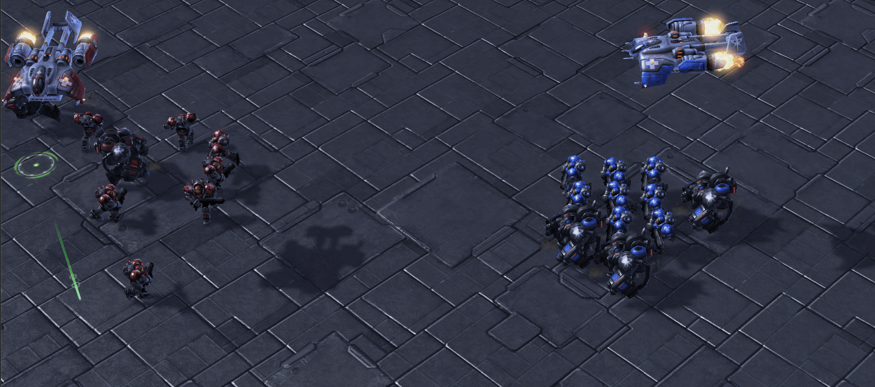
(SMAC) Samvelyan et al. (2019) (Figure 3b) is a suite of cooperative multi-agent environments based on StarCraft II. Each task consists of a single scenario with two confronting teams, one of which is controlled by the game bot and the other by our algorithm. The goal of the environment is therefore to defeat enemy team. SMAC offers 23 different scenarios with varying difficulty and number of agents. SMAC focuses on learning micromanagement of a group of agents, e.g. using terrain to your advantage as in corridor map or kite opponents as in 3s vs 3z map. Learning this behaviours requires both good exploration properties as well as solving credit assignment issue as agents need to disentangle global reward for their actions. One important property of the environment is that not all actions are available during agents decision making, e.g. attacking opponents that are out of reach. This necessitates world model to predict if the action is available or not based on latent state in order to train agents in imaginary rollouts. We use additional Bernoulli classifier similar to Discount predictor and train it on action masks provided by the environment for each agent.

4.2. Results

We adopt low data training regime from Kaiser et al. (2019) to highlight sample efficiency of the current state-of-the-art MFRL methods. We chose MAPPO Yu et al. (2021), COMA Foerster et al. (2018), QMIX Rashid et al. (2018), CommNet Sukhbaatar et al. (2016) and G2A Liu et al. (2020) as the baselines for SMAC environments and winning solution of Laurent et al. (2021) as the baseline for Flatland environment. There are three levels of difficulty both in SMAC and Flatland. In order to make up for this difference, we allocate more samples from the environment depending on its difficulty. Specifically, we use 100k, 200k and 500k samples for SMAC and 300k, 1kk and 1.5kk for Flatland. All hyperparameters, ablation study and details about the environments can be found in Appendix. We use this implementation for all baselines in SMAC except MAPPO, which implementation is provided by authors. We use authors implementation of the winning Flatland 2020 solution that can be found here.

(a) 5 agents

(b) 10 agents

(c) 15 agents

Figure 5. Experiments in Flatland environment. Y axis denotes percentage of arrived trains and X axis denotes number of steps taken in the environment.

SMAC

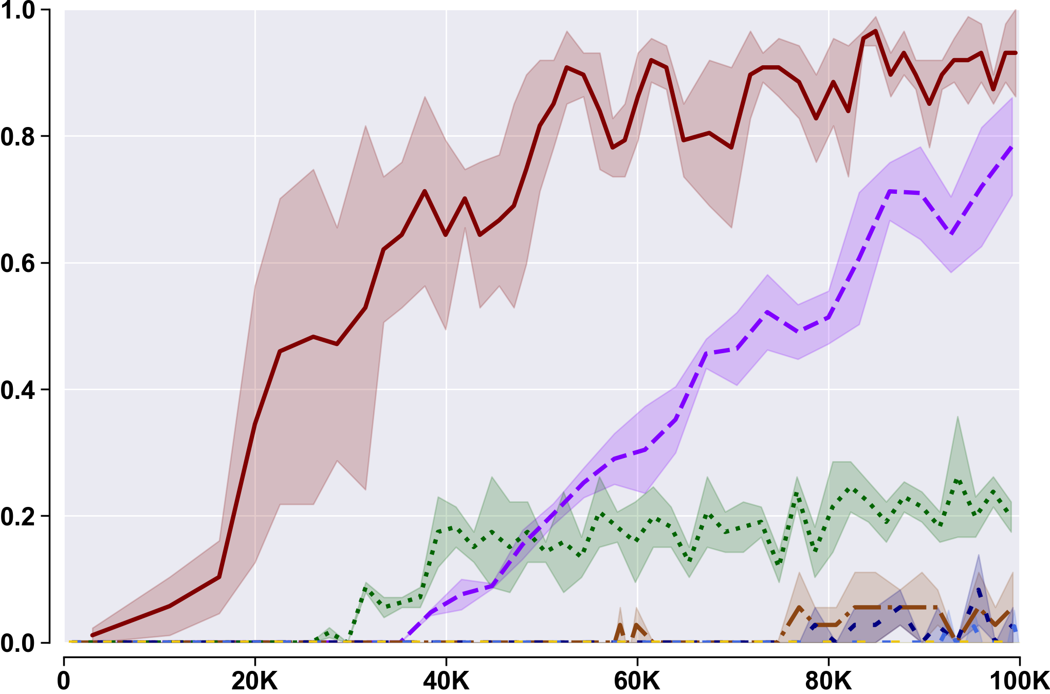
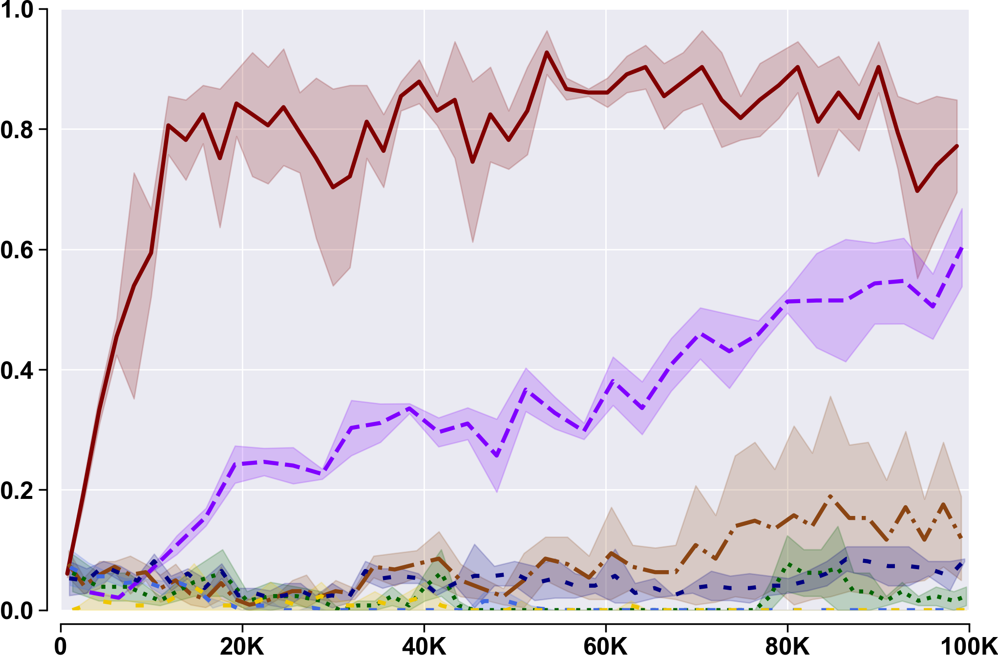
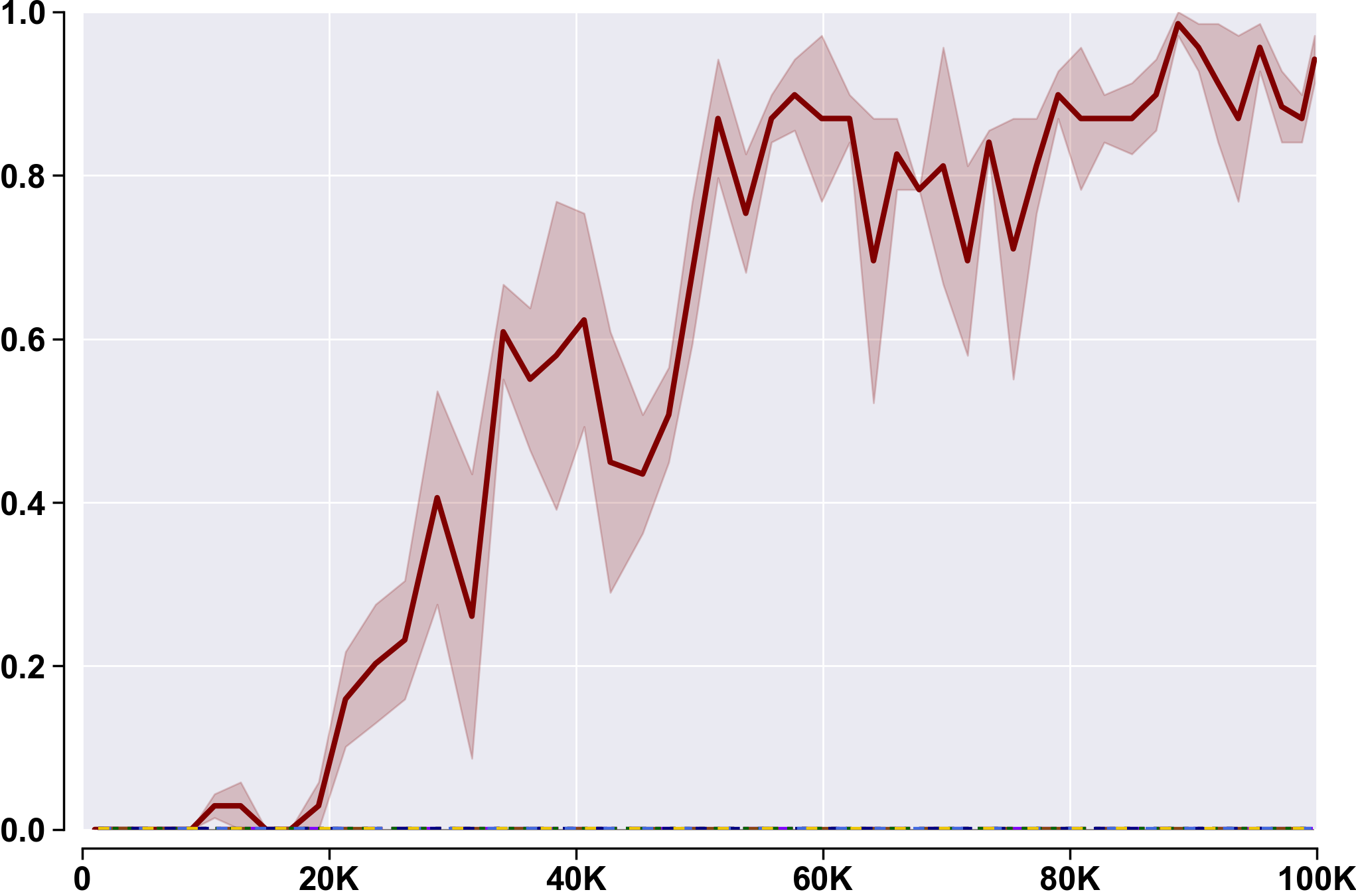
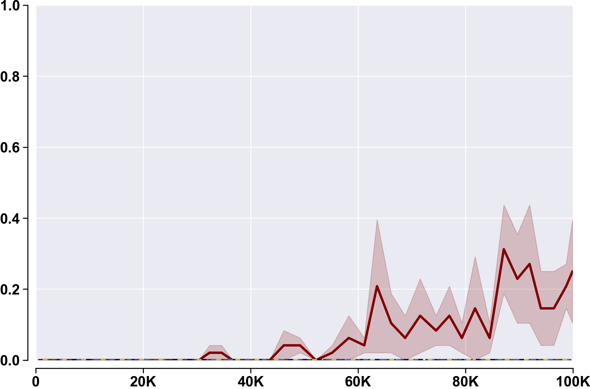
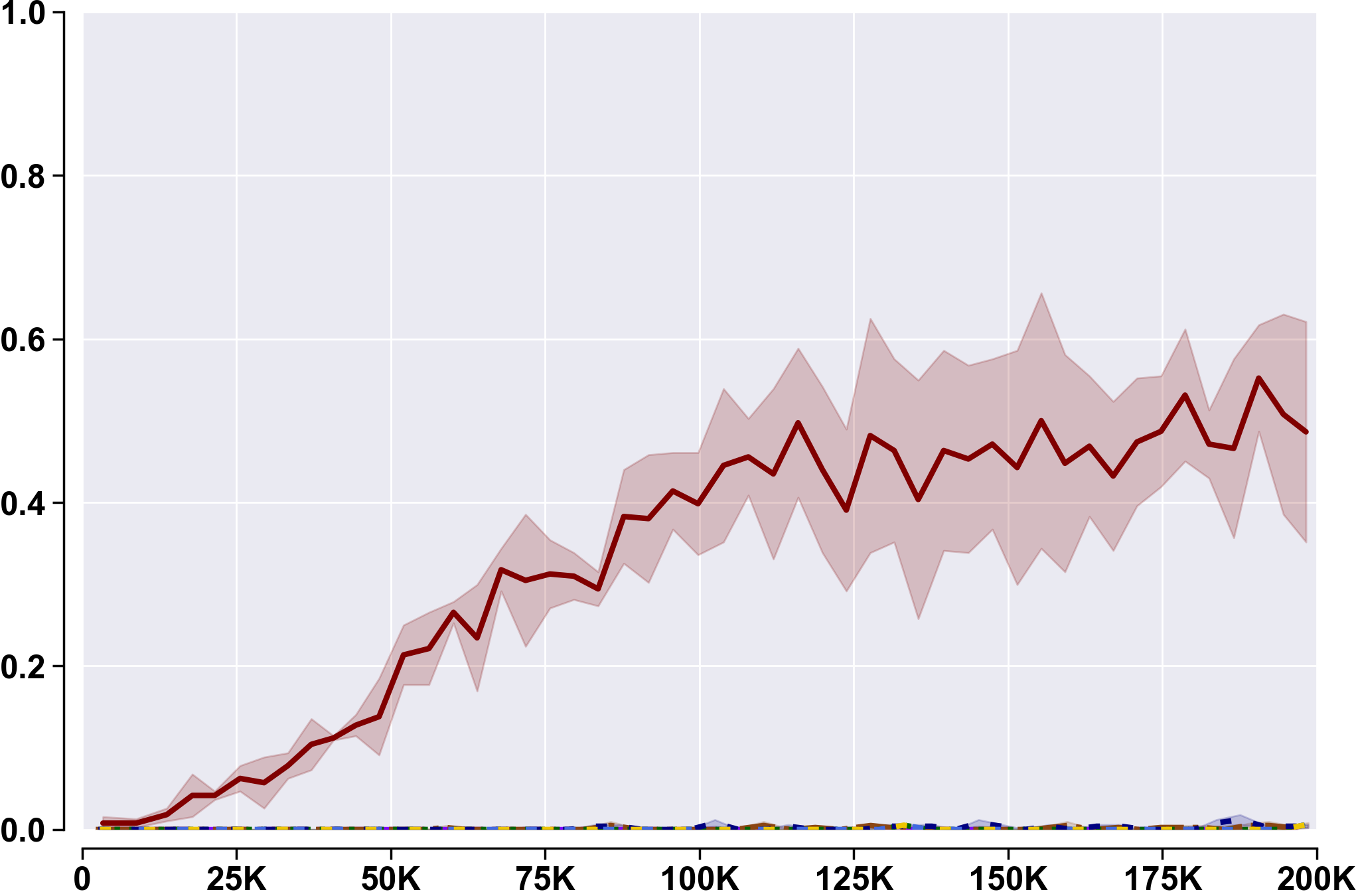
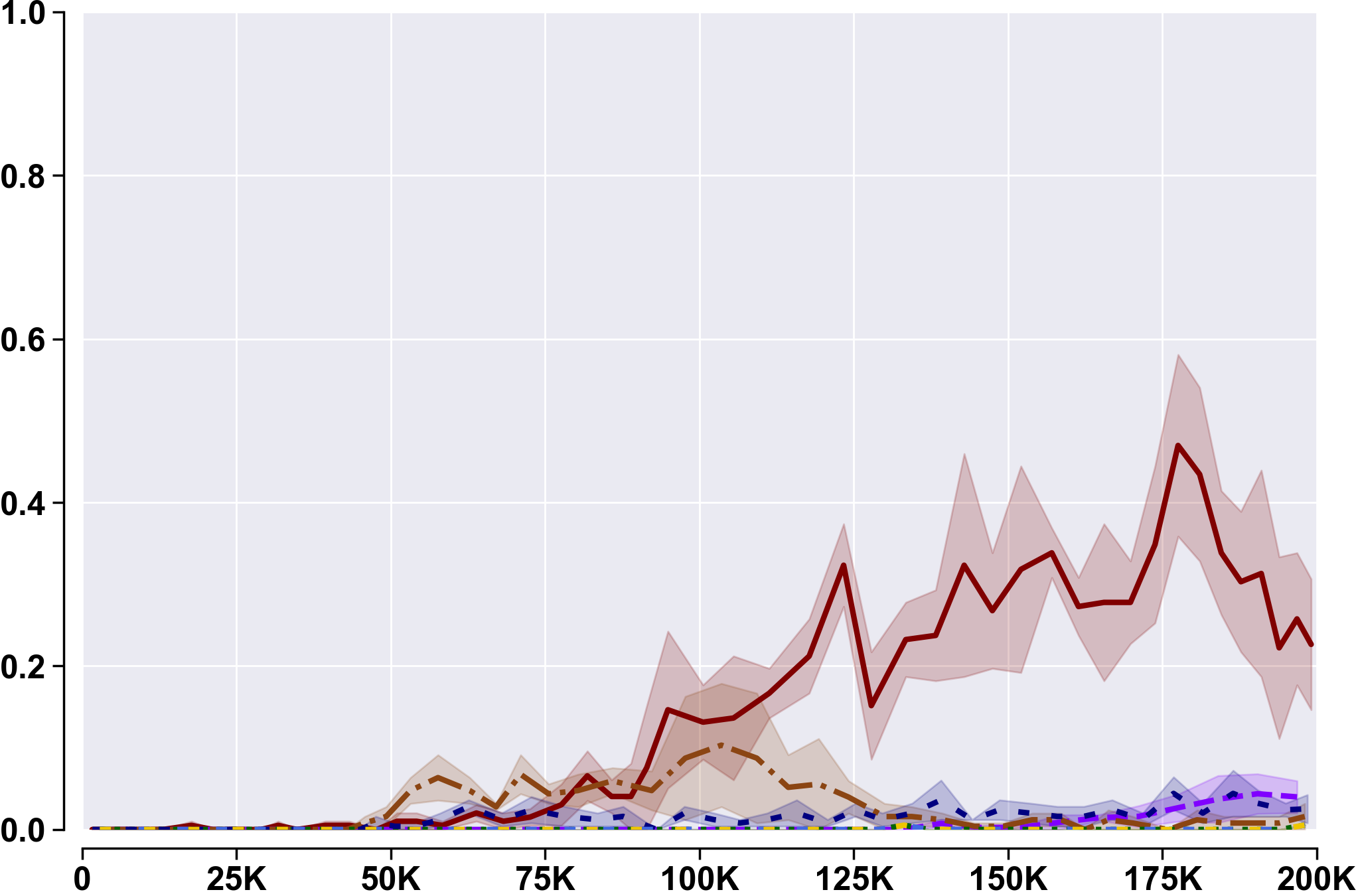
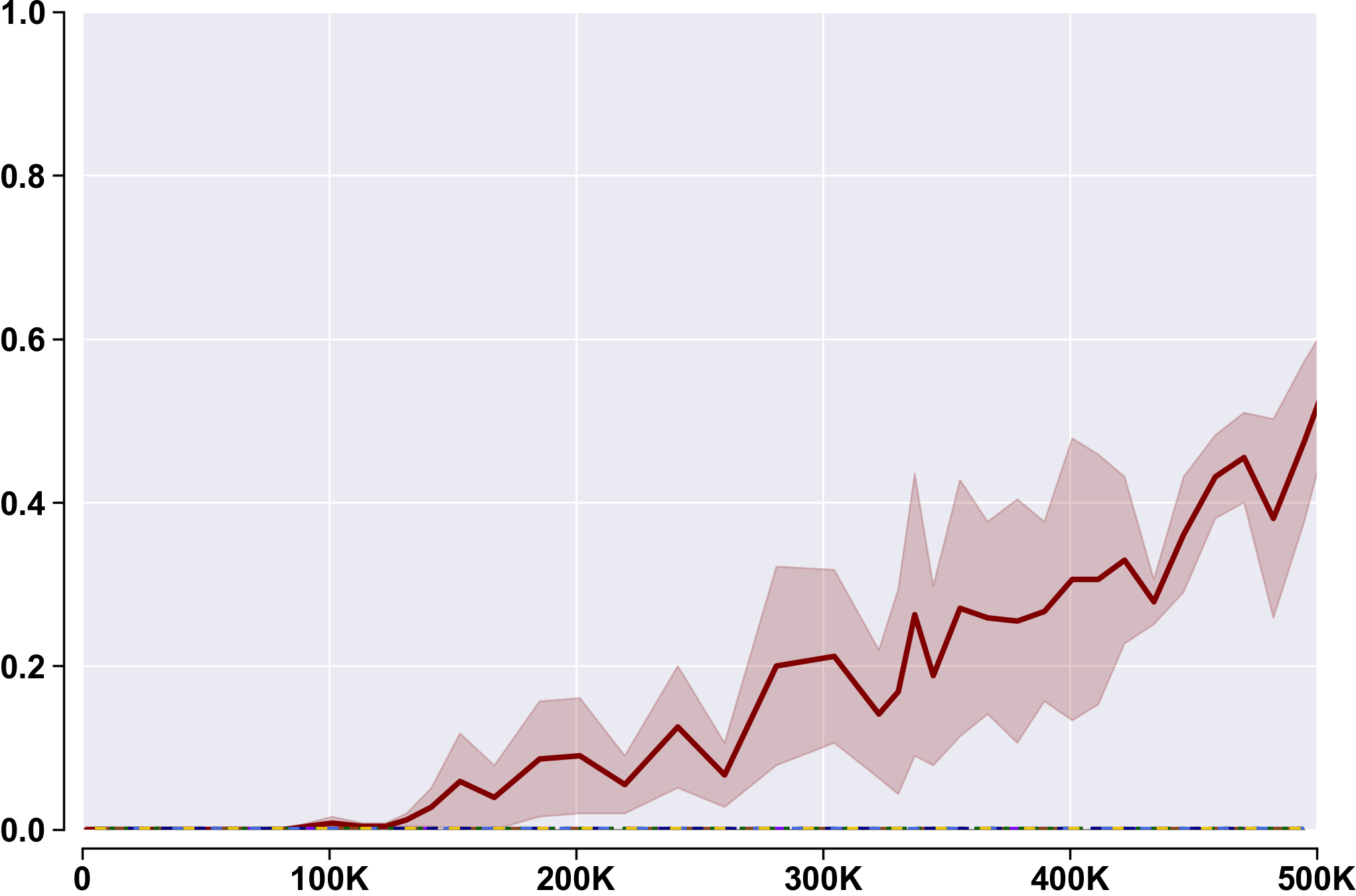
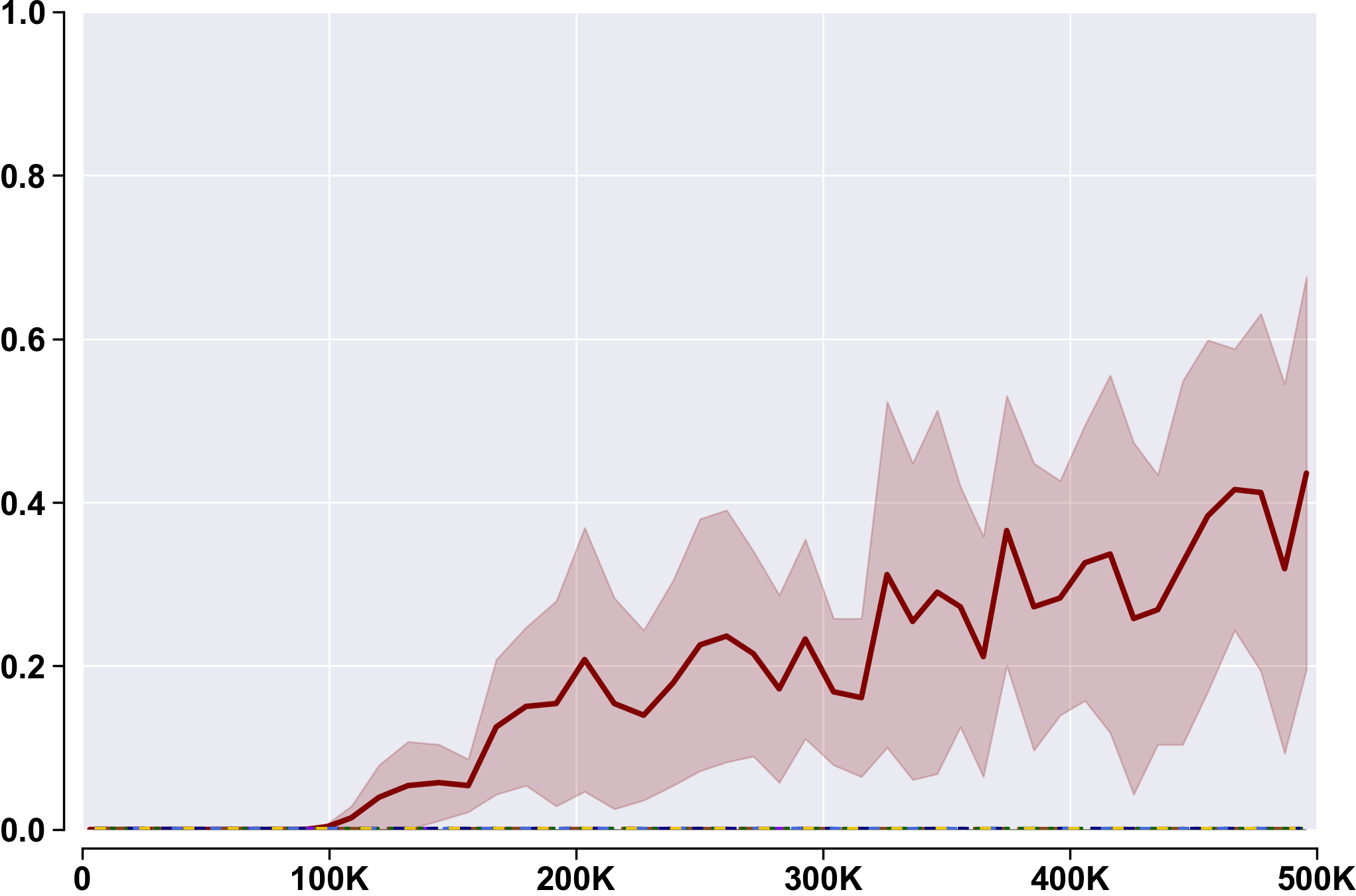
The results in SMAC environments are presented in Figure 4. We selected 8 environments out of 23 to show in the paper and the rest of the results can be found in Appendix. Specifically, we chose 4 random environments (Fig. 4 a, b, c, d) that are considered easy tasks, 2 environments (Fig. 4 e, f) with large number of agents and 2 environments (Fig. 4 g, h) with very hard tasks that require coordination. SMAC environments require coordination between all agents to complete the task, thus we did not test the locality property of our algorithm here. We can see that MAMBA outperforms all baselines in all of the environments with given number of samples. Notably, MAMBA achieves near-optimal performance on easy tasks with only 100k samples and finds winning strategy for hard and very hard tasks, winning nearly half of the episodes. On the other hand, the current state-of-the-art MFRL method MAPPO, which is able to solve all SMAC environments given large amount of samples, struggles to achieve good performance in low data regime. This highlights sample inefficiency of current MFRL approaches and shows the potential for a significant reduction in needed samples using MBRL methods. Note that communication methods G2A and CommNet are less sample efficient than MAPPO, which is likely due to additional complexity of learning how to leverage message channel. On the other hand, MAMBA encapsulates communication in a world model, which can be learned in fewer samples. Two important highlights of SMAC environments are the credit assignment problem and usage of additional information during training. We can see that MAMBA is able to disentangle global rewards and achieve good performance even without additional credit assignment techniques in most environments. We do not use additional global information during training, which is a limitation of model-based approaches discussed in Section 3.2.

Flatland

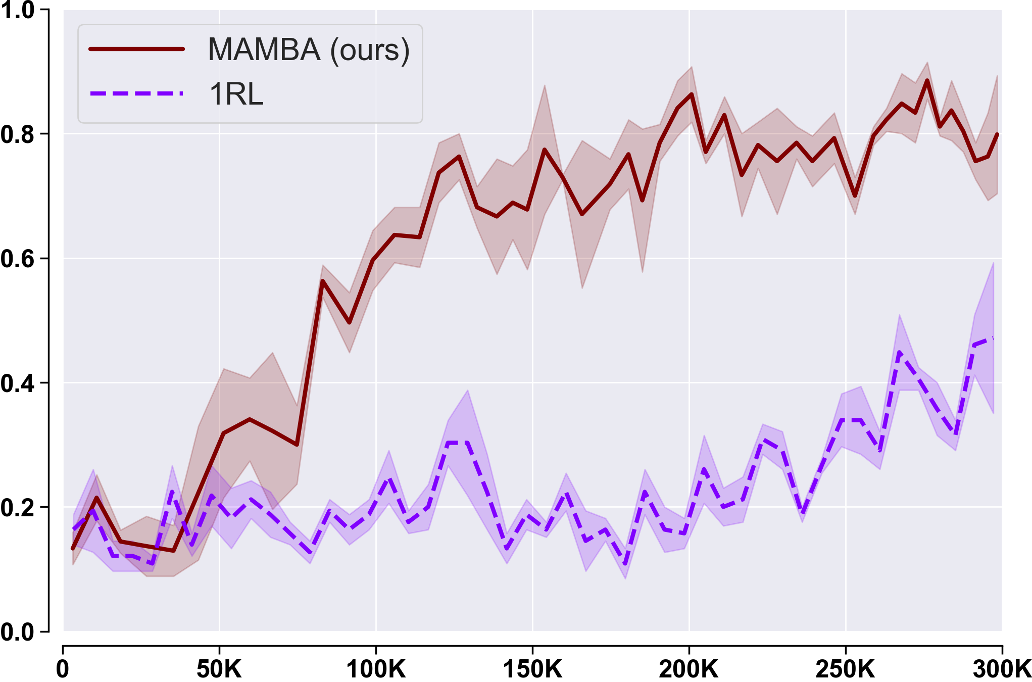
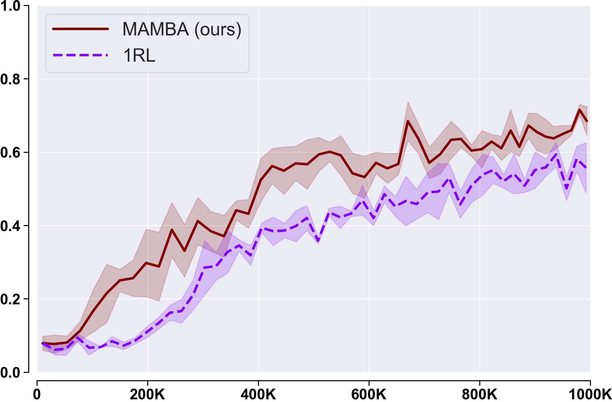
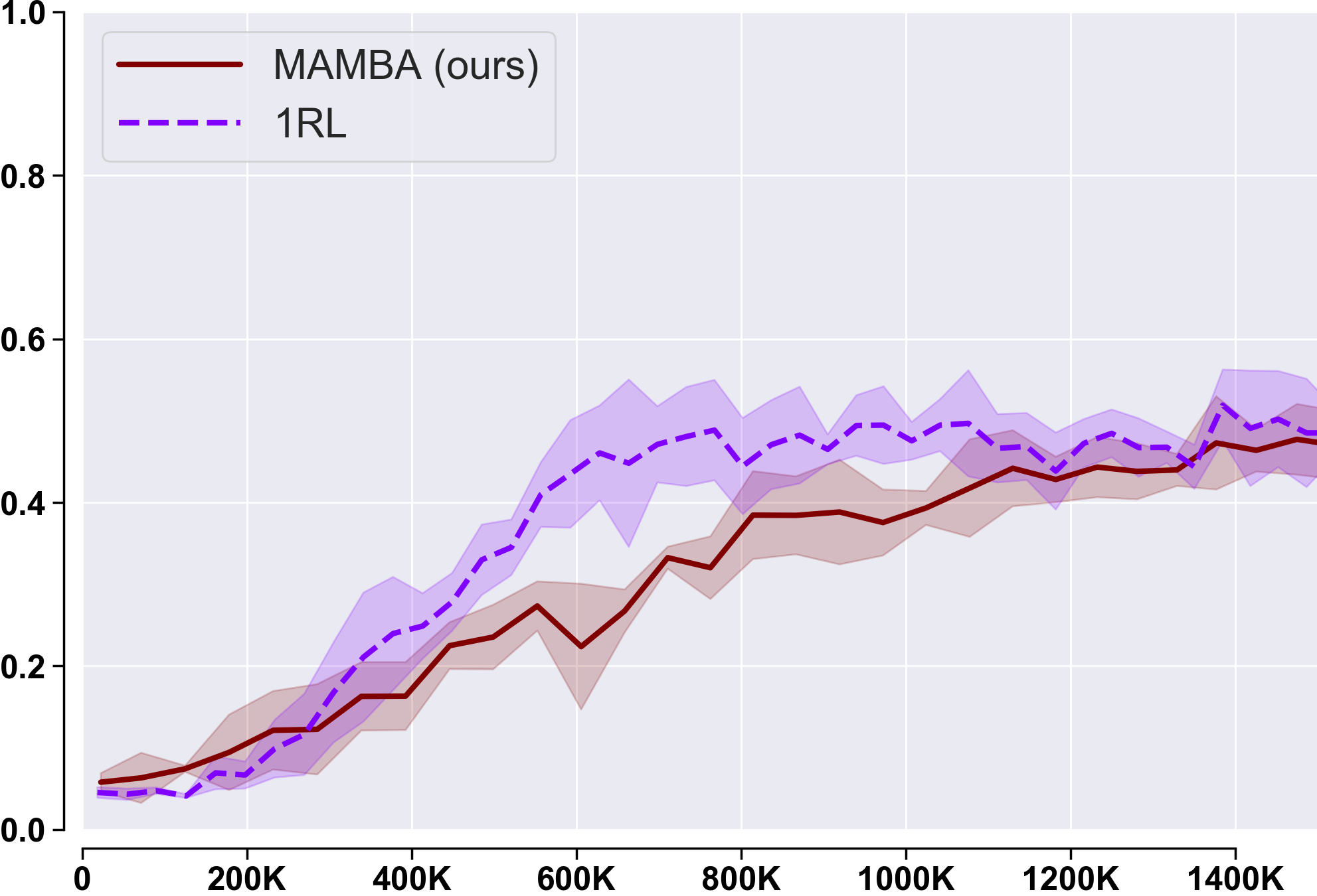
The results in Flatland environment are presented in Figure 5. We use modified version of the winning solution from the RL track of Flatland 2020 challenge Laurent et al. (2021) as our main baseline, which we will refer to as 1RL. Our only modification is disabling departure schedule, as it alters the underlying MDP of the environment. As there is no global reward in the environment, we do not compare with algorithms specific for solving credit assignment issue, e.g. COMA, QMIX and QTRAN. We also found it redundant to compare with MADDPG or communication methods such as G2A or CommNet as the winning solution employs PPO-based method with both augmented critics and communication between agents. In this environment, we use three different maps with the increasing size and number of agents. That way, we can progressively increase the difficulty of the environment and see how this affects the algorithms. Specifically, we use environments with 5, 10 and 15 agents, which turn traffic on the rail network more and more dense. This increase in difficulty affects the learning of world model as it must predict next states of all agents during training. Furthermore, during execution we provide agent messages only from its neighbours for both 1RL and MAMBA, thus limiting information about the environment only to local area of the map. Nevertheless, we can see that MAMBA can successfully achieve good performance in the 5 agents (Fig. 5 a) setting only in 300k samples while 1RL still needs more samples to improve performance. Naturally, performance decrease in 10 agents setting for both algorithms, but we can see that MAMBA still substantially outperforms 1RL method in 1 million samples (Fig. 5 b). However, we can see that sample efficiency starts to equalize compared to 5 agents setting. We hypothesize that it is easier for 1RL agents to learn on raw observations with communication than for MAMBA agents to learn from more noisy discrete latent space of the model. This issue of decaying sample efficiency is further exacerbated with the increased number of agents in the next setting. In 15 agents setting (Fig. 5 c) we can see that MAMBA is less sample efficient than 1RL but still achieves comparable performance in 1.5 million samples. We hypothesize that this decrease in sample efficiency results from the increased difficulty of the environment, which necessitates more expressive world model to approximate as well as more samples to learn.

5. Conclusion

In this paper, we present MAMBA – a MBRL method for multi-agent cooperative environments. We show the effectiveness of MAMBA in low data regime on two challenging domains of SMAC and Flatland compared to current state-of-the-art approaches, highlighting sample inefficiency of the MFRL methods. We provide architecture that can scale to a large number of agents as well as a training procedure that can learn disentangled latent space for agents. This allows us to decompose the world model by the agent, which can then be used in a decentralized manner with communication. Furthermore, we use discrete messages to facilitate decentralization and account for message channel bandwidth limitations.

6. Acknowledgements

The publication was supported by the grant for research centers in the field of AI provided by the Analytical Center for the Government of the Russian Federation (ACRF) in accordance with the agreement on the provision of subsidies (identifier of the agreement 000000D730321P5Q0002) and the agreement with HSE University No. 70-2021-00139. This research was supported in part through computational resources of HPC facilities at HSE University Kostenetskiy et al. (2021).

Appendix A Hyperparameters

We use random search with 50 runs to find best hyperparameters on the Flatland environment with 5 agents and use them for all Flatland environments. Similarly, we use random search with 50 runs for SMAC on 3s vs 3z environment. Specifically, we sample values for search from the following grid: Actor Learning rate from [1e-4, 5e-4, 2e-4], Critic Learning rate from [1e-4, 5e-4, 2e-4], Model Learning rate from [1e-4, 2e-4, 1e-3], Model number of epochs from [20, 40, 60], PPO epochs per update $[3,5,10]$, Rollout horizon from [5, 10, 15].

Hyperparameter	Flatland	SMAC
PPO
Batch size	2000
GAE $\lambda$	0.95
Entropy coefficient	0.001
Entropy annealing	0.99998
Number of updates	4
Epochs per update	5
Update clipping parameter	0.2
Actor Learning rate	5e-4
Critic Learning rate	5e-4
$\gamma$	0.99
Model
Model Learning rate	2e-4
Number of epochs	40	60
Number of sampled rollouts	40
Sequence length	50	20
Rollout horizon $H$	15
Buffer size	5e5	2.5e5
Number of categoricals	32
Number of classes	32
KL balancing entropy weight	0.2
KL balancing cross entropy weight	0.8
Common
Gradient clipping	100
Trajectories between updates	1
Hidden size	400	256

Table 1. Hyperparameters for MAMBA.

Appendix B Environments

We use authors implementation of SMAC environments with default settings. For Flatland environments, we use Flatland class Mohanty et al. (2020) to generate environments with parameters shown in Table 2

Flatland parameter	5 agents	10 agents	15 agents
height	35	35	40
width	35	35	45
n_agents	5	10	15
n_cities	3	4	5
grid_distribution_of_cities	False	False	False
max_rails_between_cities	2	2	2
max_rail_in_cities	4	4	4
malfunction_rate	1./100	1./150	1./200

Table 2. Parameters for Flatland environments

Appendix C Ablation study

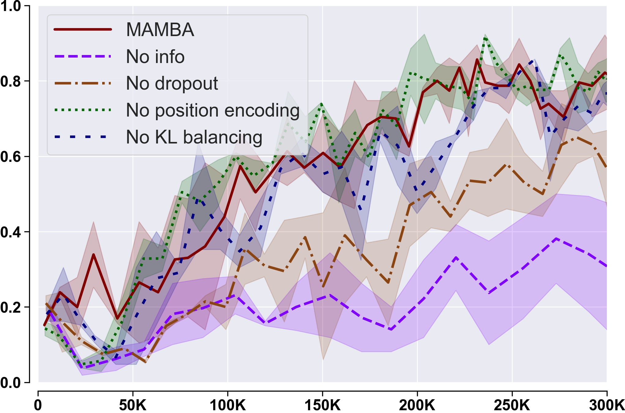
We conduct several ablation experiments in Flatland environment with 5 agents. The results with algorithms executed with 3 random seeds are reported in Figure 6. Specifically, we test whether disabling the information loss $\mathcal{L}_{\text{info}}$, KL balancing, dropout rate $p$ in Communication Block or position encoding in Communication Block degrades final performance. Notably, both position encoding and KL balancing are not important for overall performance while dropout and $\mathcal{L}_{\text{info}}$ have a great impact on learning.

Figure 6. Ablation study in Flatland

Appendix D SMAC results

We report final performance of the algorithms for all SMAC environments in Table 3.

Map	Number of samples	MAMBA	MAPPO	QMIX	COMA	QTRAN	G2A	CommNet
2m_vs_1z	100k	93(1)	89(4)	57(12)	0	57(1)	0	0
3m	100k	91(2)	64(3)	53(7)	45(6)	39(4)	8(2)	14(4)
2s_vs_1sc	100k	98(1)	78(9)	10(9)	18(2)	4(3)	11(6)	1(2)
2s3z	100k	69(1)	3	24(4)	0	16(7)	1(2)	1
3s_vs_3z	100k	90	0	0	0	0	0	0
3s_vs_4z	100k	26(4)	0	0	0	0	0	0
so_many_baneling	100k	83(7)	60(8)	23(9)	17(4)	7(1)	0	0
8m	100k	80(3)	45(7)	22(11)	21(1)	33(6)	9(1)	2
MMM	100k	48(11)	2(1)	4(3)	0	0	0	0
1c3s5z	100k	85(8)	3(2)	32(11)	0	5(4)	0	0
bane_vs_bane	100k	39(20)	93(2)	52(12)	48(13)	54(9)	56(11)	28(40)
3s_vs_5z	200k	3(4)	0	0	0	0	0	0
2c_vs_64zg	200k	8(4)	0	0	1(2)	0	0	0
8m_vs_9m	200k	50(14)	0	0	0	0	0	0
25m	200k	27(8)	2(2)	8(8)	0	3(1)	0	0
5m_vs_6m	200k	24(10)	0	0	0	0	0	0
3s5z	200k	17(5)	0	0	0	0	0	0
10m_vs_11m	200k	54(5)	2	1(1)	0	0	0	0
MMM2	500k	23(3)	0	0	0	0	0	0
3s5z_vs_3s6z	500k	44(25)	0	0	0	0	0	0
27m_vs_30m	500k	1(1)	0	0	0	0	0	0
6h_vs_8z	500k	1(2)	0	0	0	0	0	0
corridor	500k	39(10)	0	0	0	0	0	0

Table 3. Mean and std of winning percentage after learning for specified number of samples for 3 runs in SMAC environments.

References

- (1)
- Agarwal et al. (2020) Alekh Agarwal, Sham Kakade, and Lin F Yang. 2020. Model-based reinforcement learning with a generative model is minimax optimal. In Conference on Learning Theory. PMLR, 67–83.
- Andrychowicz et al. (2017) Marcin Andrychowicz, Filip Wolski, Alex Ray, Jonas Schneider, Rachel Fong, Peter Welinder, Bob McGrew, Josh Tobin, Pieter Abbeel, and Wojciech Zaremba. 2017. Hindsight experience replay. arXiv preprint arXiv:1707.01495 (2017).
- Azar et al. (2021) Ahmad Taher Azar, Anis Koubaa, Nada Ali Mohamed, Habiba A Ibrahim, Zahra Fathy Ibrahim, Muhammad Kazim, Adel Ammar, Bilel Benjdira, Alaa M Khamis, Ibrahim A Hameed, et al. 2021. Drone Deep Reinforcement Learning: A Review. Electronics 10, 9 (2021), 999.
- Azar et al. (2013) Mohammad Gheshlaghi Azar, Rémi Munos, and Hilbert J Kappen. 2013. Minimax PAC bounds on the sample complexity of reinforcement learning with a generative model. Machine learning 91, 3 (2013), 325–349.
- Bahdanau et al. (2014) Dzmitry Bahdanau, Kyunghyun Cho, and Yoshua Bengio. 2014. Neural machine translation by jointly learning to align and translate. arXiv preprint arXiv:1409.0473 (2014).
- Bengio et al. (2013) Yoshua Bengio, Nicholas Léonard, and Aaron Courville. 2013. Estimating or propagating gradients through stochastic neurons for conditional computation. arXiv preprint arXiv:1308.3432 (2013).
- Berner et al. (2019) Christopher Berner, Greg Brockman, Brooke Chan, Vicki Cheung, Przemysław D\kebiak, Christy Dennison, David Farhi, Quirin Fischer, Shariq Hashme, Chris Hesse, et al. 2019. Dota 2 with Large Scale Deep Reinforcement Learning. arXiv preprint arXiv:1912.06680 (2019).
- Blumenkamp and Prorok (2020) Jan Blumenkamp and Amanda Prorok. 2020. The emergence of adversarial communication in multi-agent reinforcement learning. arXiv preprint arXiv:2008.02616 (2020).
- Cao et al. (2018) Kris Cao, Angeliki Lazaridou, Marc Lanctot, Joel Z Leibo, Karl Tuyls, and Stephen Clark. 2018. Emergent communication through negotiation. arXiv preprint arXiv:1804.03980 (2018).
- Chen et al. (2016) Xi Chen, Yan Duan, Rein Houthooft, John Schulman, Ilya Sutskever, and Pieter Abbeel. 2016. Infogan: Interpretable representation learning by information maximizing generative adversarial nets. In Proceedings of the 30th International Conference on Neural Information Processing Systems. 2180–2188.
- Cho et al. (2014) Kyunghyun Cho, Bart Van Merriënboer, Caglar Gulcehre, Dzmitry Bahdanau, Fethi Bougares, Holger Schwenk, and Yoshua Bengio. 2014. Learning phrase representations using RNN encoder-decoder for statistical machine translation. arXiv preprint arXiv:1406.1078 (2014).
- Das et al. (2019) Abhishek Das, Théophile Gervet, Joshua Romoff, Dhruv Batra, Devi Parikh, Mike Rabbat, and Joelle Pineau. 2019. Tarmac: Targeted multi-agent communication. In International Conference on Machine Learning. PMLR, 1538–1546.
- de Witt et al. (2020) Christian Schroeder de Witt, Tarun Gupta, Denys Makoviichuk, Viktor Makoviychuk, Philip HS Torr, Mingfei Sun, and Shimon Whiteson. 2020. Is Independent Learning All You Need in the StarCraft Multi-Agent Challenge? arXiv preprint arXiv:2011.09533 (2020).
- Desjardins and Chaib-Draa (2011) Charles Desjardins and Brahim Chaib-Draa. 2011. Cooperative adaptive cruise control: A reinforcement learning approach. IEEE Transactions on intelligent transportation systems 12, 4 (2011), 1248–1260.
- Devlin et al. (2018) Jacob Devlin, Ming-Wei Chang, Kenton Lee, and Kristina Toutanova. 2018. Bert: Pre-training of deep bidirectional transformers for language understanding. arXiv preprint arXiv:1810.04805 (2018).
- Dosovitskiy et al. (2020) Alexey Dosovitskiy, Lucas Beyer, Alexander Kolesnikov, Dirk Weissenborn, Xiaohua Zhai, Thomas Unterthiner, Mostafa Dehghani, Matthias Minderer, Georg Heigold, Sylvain Gelly, et al. 2020. An image is worth 16x16 words: Transformers for image recognition at scale. arXiv preprint arXiv:2010.11929 (2020).
- Ellis and Larsen-Freeman (2006) Nick C Ellis and Diane Larsen-Freeman. 2006. Language emergence: Implications for applied linguistics—Introduction to the special issue. Applied linguistics 27, 4 (2006), 558–589.
- Foerster et al. (2018) Jakob Foerster, Gregory Farquhar, Triantafyllos Afouras, Nantas Nardelli, and Shimon Whiteson. 2018. Counterfactual multi-agent policy gradients. In Proceedings of the AAAI Conference on Artificial Intelligence, Vol. 32.
- Foerster et al. (2017) Jakob Foerster, Nantas Nardelli, Gregory Farquhar, Triantafyllos Afouras, Philip HS Torr, Pushmeet Kohli, and Shimon Whiteson. 2017. Stabilising experience replay for deep multi-agent reinforcement learning. In International conference on machine learning. PMLR, 1146–1155.
- Foerster et al. (2016) Jakob N Foerster, Yannis M Assael, Nando De Freitas, and Shimon Whiteson. 2016. Learning to communicate with deep multi-agent reinforcement learning. arXiv preprint arXiv:1605.06676 (2016).
- Gronauer and Diepold (2021) Sven Gronauer and Klaus Diepold. 2021. Multi-agent deep reinforcement learning: a survey. Artificial Intelligence Review (2021), 1–49.
- Gupta et al. (2017) Jayesh K Gupta, Maxim Egorov, and Mykel Kochenderfer. 2017. Cooperative multi-agent control using deep reinforcement learning. In International Conference on Autonomous Agents and Multiagent Systems. Springer, 66–83.
- Hafner et al. (2019a) Danijar Hafner, Timothy Lillicrap, Jimmy Ba, and Mohammad Norouzi. 2019a. Dream to control: Learning behaviors by latent imagination. arXiv preprint arXiv:1912.01603 (2019).
- Hafner et al. (2019b) Danijar Hafner, Timothy Lillicrap, Ian Fischer, Ruben Villegas, David Ha, Honglak Lee, and James Davidson. 2019b. Learning latent dynamics for planning from pixels. In International Conference on Machine Learning. PMLR, 2555–2565.
- Hafner et al. (2020) Danijar Hafner, Timothy Lillicrap, Mohammad Norouzi, and Jimmy Ba. 2020. Mastering atari with discrete world models. arXiv preprint arXiv:2010.02193 (2020).
- Havrylov and Titov (2017) Serhii Havrylov and Ivan Titov. 2017. Emergence of language with multi-agent games: Learning to communicate with sequences of symbols. arXiv preprint arXiv:1705.11192 (2017).
- Hernandez-Leal et al. (2017) Pablo Hernandez-Leal, Michael Kaisers, Tim Baarslag, and Enrique Munoz de Cote. 2017. A survey of learning in multiagent environments: Dealing with non-stationarity. arXiv preprint arXiv:1707.09183 (2017).
- Higgins et al. (2016) Irina Higgins, Loic Matthey, Arka Pal, Christopher Burgess, Xavier Glorot, Matthew Botvinick, Shakir Mohamed, and Alexander Lerchner. 2016. beta-vae: Learning basic visual concepts with a constrained variational framework. (2016).
- Hochreiter and Schmidhuber (1997) Sepp Hochreiter and Jürgen Schmidhuber. 1997. Long short-term memory. Neural computation 9, 8 (1997), 1735–1780.
- Iqbal and Sha (2019) Shariq Iqbal and Fei Sha. 2019. Actor-attention-critic for multi-agent reinforcement learning. In International Conference on Machine Learning. PMLR, 2961–2970.
- Janner et al. (2019) Michael Janner, Justin Fu, Marvin Zhang, and Sergey Levine. 2019. When to trust your model: Model-based policy optimization. arXiv preprint arXiv:1906.08253 (2019).
- Jiang and Lu (2018) Jiechuan Jiang and Zongqing Lu. 2018. Learning attentional communication for multi-agent cooperation. arXiv preprint arXiv:1805.07733 (2018).
- Kaiser et al. (2019) Lukasz Kaiser, Mohammad Babaeizadeh, Piotr Milos, Blazej Osinski, Roy H Campbell, Konrad Czechowski, Dumitru Erhan, Chelsea Finn, Piotr Kozakowski, Sergey Levine, et al. 2019. Model-based reinforcement learning for atari. arXiv preprint arXiv:1903.00374 (2019).
- Kingma and Ba (2014) Diederik P Kingma and Jimmy Ba. 2014. Adam: A method for stochastic optimization. arXiv preprint arXiv:1412.6980 (2014).
- Kingma and Welling (2013) Diederik P Kingma and Max Welling. 2013. Auto-encoding variational bayes. arXiv preprint arXiv:1312.6114 (2013).
- Kostenetskiy et al. (2021) PS Kostenetskiy, RA Chulkevich, and VI Kozyrev. 2021. HPC Resources of the Higher School of Economics. In Journal of Physics: Conference Series, Vol. 1740. IOP Publishing, 012050.
- Kostrikov et al. (2018) Ilya Kostrikov, Kumar Krishna Agrawal, Debidatta Dwibedi, Sergey Levine, and Jonathan Tompson. 2018. Discriminator-actor-critic: Addressing sample inefficiency and reward bias in adversarial imitation learning. arXiv preprint arXiv:1809.02925 (2018).
- Kraemer and Banerjee (2016) Landon Kraemer and Bikramjit Banerjee. 2016. Multi-agent reinforcement learning as a rehearsal for decentralized planning. Neurocomputing 190 (2016), 82–94.
- Krupnik et al. (2020) Orr Krupnik, Igor Mordatch, and Aviv Tamar. 2020. Multi-agent reinforcement learning with multi-step generative models. In Conference on Robot Learning. PMLR, 776–790.
- Laurent et al. (2021) Florian Laurent, Manuel Schneider, Christian Scheller, Jeremy Watson, Jiaoyang Li, Zhe Chen, Yi Zheng, Shao-Hung Chan, Konstantin Makhnev, Oleg Svidchenko, et al. 2021. Flatland Competition 2020: MAPF and MARL for Efficient Train Coordination on a Grid World. arXiv preprint arXiv:2103.16511 (2021).
- Laurent et al. (2011) Guillaume J Laurent, Laëtitia Matignon, Le Fort-Piat, et al. 2011. The world of independent learners is not Markovian. International Journal of Knowledge-based and Intelligent Engineering Systems 15, 1 (2011), 55–64.
- Lazaridou et al. (2016) Angeliki Lazaridou, Alexander Peysakhovich, and Marco Baroni. 2016. Multi-agent cooperation and the emergence of (natural) language. arXiv preprint arXiv:1612.07182 (2016).
- Li et al. (2020) Gen Li, Yuting Wei, Yuejie Chi, Yuantao Gu, and Yuxin Chen. 2020. Breaking the sample size barrier in model-based reinforcement learning with a generative model. Advances in neural information processing systems 33 (2020).
- Littman (1994) Michael L Littman. 1994. Markov games as a framework for multi-agent reinforcement learning. In Machine learning proceedings 1994. Elsevier, 157–163.
- Liu et al. (2021) Qinghua Liu, Tiancheng Yu, Yu Bai, and Chi Jin. 2021. A sharp analysis of model-based reinforcement learning with self-play. In International Conference on Machine Learning. PMLR, 7001–7010.
- Liu et al. (2020) Yong Liu, Weixun Wang, Yujing Hu, Jianye Hao, Xingguo Chen, and Yang Gao. 2020. Multi-agent game abstraction via graph attention neural network. In Proceedings of the AAAI Conference on Artificial Intelligence, Vol. 34. 7211–7218.
- Lowe et al. (2017) Ryan Lowe, Yi Wu, Aviv Tamar, Jean Harb, Pieter Abbeel, and Igor Mordatch. 2017. Multi-agent actor-critic for mixed cooperative-competitive environments. arXiv preprint arXiv:1706.02275 (2017).
- Maes (1993) Pattie Maes. 1993. Modeling adaptive autonomous agents. Artificial life 1, 1_2 (1993), 135–162.
- Mnih et al. (2016) Volodymyr Mnih, Adria Puigdomenech Badia, Mehdi Mirza, Alex Graves, Timothy Lillicrap, Tim Harley, David Silver, and Koray Kavukcuoglu. 2016. Asynchronous methods for deep reinforcement learning. In International conference on machine learning. 1928–1937.
- Mohanty et al. (2020) Sharada Mohanty, Erik Nygren, Florian Laurent, Manuel Schneider, Christian Scheller, Nilabha Bhattacharya, Jeremy Watson, Adrian Egli, Christian Eichenberger, Christian Baumberger, et al. 2020. Flatland-RL: Multi-agent reinforcement learning on trains. arXiv preprint arXiv:2012.05893 (2020).
- Noukhovitch et al. (2021) Michael Noukhovitch, Travis LaCroix, Angeliki Lazaridou, and Aaron Courville. 2021. Emergent Communication under Competition. arXiv preprint arXiv:2101.10276 (2021).
- Oord et al. (2017) Aaron van den Oord, Oriol Vinyals, and Koray Kavukcuoglu. 2017. Neural discrete representation learning. arXiv preprint arXiv:1711.00937 (2017).
- Precup (2000) Doina Precup. 2000. Eligibility traces for off-policy policy evaluation. Computer Science Department Faculty Publication Series (2000), 80.
- Rashid et al. (2018) Tabish Rashid, Mikayel Samvelyan, Christian Schroeder, Gregory Farquhar, Jakob Foerster, and Shimon Whiteson. 2018. Qmix: Monotonic value function factorisation for deep multi-agent reinforcement learning. In International Conference on Machine Learning. PMLR, 4295–4304.
- Razavi et al. (2019) Ali Razavi, Aaron van den Oord, and Oriol Vinyals. 2019. Generating diverse high-fidelity images with vq-vae-2. In Advances in neural information processing systems. 14866–14876.
- Samvelyan et al. (2019) Mikayel Samvelyan, Tabish Rashid, Christian Schroeder de Witt, Gregory Farquhar, Nantas Nardelli, Tim G. J. Rudner, Chia-Man Hung, Philiph H. S. Torr, Jakob Foerster, and Shimon Whiteson. 2019. The StarCraft Multi-Agent Challenge. CoRR abs/1902.04043 (2019).
- Schrittwieser et al. (2020) Julian Schrittwieser, Ioannis Antonoglou, Thomas Hubert, Karen Simonyan, Laurent Sifre, Simon Schmitt, Arthur Guez, Edward Lockhart, Demis Hassabis, Thore Graepel, et al. 2020. Mastering atari, go, chess and shogi by planning with a learned model. Nature 588, 7839 (2020), 604–609.
- Schulman et al. (2015) John Schulman, Philipp Moritz, Sergey Levine, Michael Jordan, and Pieter Abbeel. 2015. High-dimensional continuous control using generalized advantage estimation. arXiv preprint arXiv:1506.02438 (2015).
- Schulman et al. (2017) John Schulman, Filip Wolski, Prafulla Dhariwal, Alec Radford, and Oleg Klimov. 2017. Proximal policy optimization algorithms. arXiv preprint arXiv:1707.06347 (2017).
- Schwarting et al. (2021) Wilko Schwarting, Tim Seyde, Igor Gilitschenski, Lucas Liebenwein, Ryan Sander, Sertac Karaman, and Daniela Rus. 2021. Deep latent competition: Learning to race using visual control policies in latent space. arXiv preprint arXiv:2102.09812 (2021).
- Shen et al. (2018) Tao Shen, Tianyi Zhou, Guodong Long, Jing Jiang, Sen Wang, and Chengqi Zhang. 2018. Reinforced self-attention network: a hybrid of hard and soft attention for sequence modeling. arXiv preprint arXiv:1801.10296 (2018).
- Silver et al. (2016) David Silver, Aja Huang, Christopher J. Maddison, Arthur Guez, Laurent Sifre, George van den Driessche, Julian Schrittwieser, Ioannis Antonoglou, Veda Panneershelvam, Marc Lanctot, Sander Dieleman, Dominik Grewe, John Nham, Nal Kalchbrenner, Ilya Sutskever, Timothy Lillicrap, Madeleine Leach, Koray Kavukcuoglu, Thore Graepel, and Demis Hassabis. 2016. Mastering the game of Go with deep neural networks and tree search. Nature 529 (2016), 484–503. http://www.nature.com/nature/journal/v529/n7587/full/nature16961.html
- Singh et al. (2018) Amanpreet Singh, Tushar Jain, and Sainbayar Sukhbaatar. 2018. Learning when to communicate at scale in multiagent cooperative and competitive tasks. arXiv preprint arXiv:1812.09755 (2018).
- Son et al. (2019) Kyunghwan Son, Daewoo Kim, Wan Ju Kang, David Earl Hostallero, and Yung Yi. 2019. Qtran: Learning to factorize with transformation for cooperative multi-agent reinforcement learning. In International Conference on Machine Learning. PMLR, 5887–5896.
- Srivastava et al. (2014) Nitish Srivastava, Geoffrey Hinton, Alex Krizhevsky, Ilya Sutskever, and Ruslan Salakhutdinov. 2014. Dropout: a simple way to prevent neural networks from overfitting. The journal of machine learning research 15, 1 (2014), 1929–1958.
- Sukhbaatar et al. (2016) Sainbayar Sukhbaatar, Rob Fergus, et al. 2016. Learning multiagent communication with backpropagation. Advances in neural information processing systems 29 (2016), 2244–2252.
- Sunehag et al. (2017) Peter Sunehag, Guy Lever, Audrunas Gruslys, Wojciech Marian Czarnecki, Vinicius Zambaldi, Max Jaderberg, Marc Lanctot, Nicolas Sonnerat, Joel Z Leibo, Karl Tuyls, et al. 2017. Value-decomposition networks for cooperative multi-agent learning. arXiv preprint arXiv:1706.05296 (2017).
- Sutton (1991) Richard S Sutton. 1991. Dyna, an integrated architecture for learning, planning, and reacting. ACM Sigart Bulletin 2, 4 (1991), 160–163.
- Sutton and Barto (2018) Richard S Sutton and Andrew G Barto. 2018. Reinforcement learning: An introduction. MIT press.
- Tan (1993) Ming Tan. 1993. Multi-agent reinforcement learning: Independent vs. cooperative agents. In Proceedings of the tenth international conference on machine learning. 330–337.
- Vaswani et al. (2017) Ashish Vaswani, Noam Shazeer, Niki Parmar, Jakob Uszkoreit, Llion Jones, Aidan N Gomez, Łukasz Kaiser, and Illia Polosukhin. 2017. Attention is all you need. In Advances in neural information processing systems. 5998–6008.
- Vinyals et al. (2019) Oriol Vinyals, Igor Babuschkin, Wojciech M Czarnecki, Michaël Mathieu, Andrew Dudzik, Junyoung Chung, David H Choi, Richard Powell, Timo Ewalds, Petko Georgiev, et al. 2019. Grandmaster level in StarCraft II using multi-agent reinforcement learning. Nature 575, 7782 (2019), 350–354.
- Wang et al. (2020b) Weixun Wang, Tianpei Yang, Yong Liu, Jianye Hao, Xiaotian Hao, Yujing Hu, Yingfeng Chen, Changjie Fan, and Yang Gao. 2020b. From few to more: Large-scale dynamic multiagent curriculum learning. In Proceedings of the AAAI Conference on Artificial Intelligence, Vol. 34. 7293–7300.
- Wang et al. (2020a) Yihan Wang, Beining Han, Tonghan Wang, Heng Dong, and Chongjie Zhang. 2020a. Off-policy multi-agent decomposed policy gradients. arXiv preprint arXiv:2007.12322 (2020).
- Watkins and Dayan (1992) Christopher JCH Watkins and Peter Dayan. 1992. Q-learning. Machine learning 8, 3-4 (1992), 279–292.
- Williams (1992) Ronald J Williams. 1992. Simple statistical gradient-following algorithms for connectionist reinforcement learning. Machine learning 8, 3 (1992), 229–256.
- Wolpert and Tumer (2002) David H Wolpert and Kagan Tumer. 2002. Optimal payoff functions for members of collectives. In Modeling complexity in economic and social systems. World Scientific, 355–369.
- Yu et al. (2021) Chao Yu, Akash Velu, Eugene Vinitsky, Yu Wang, Alexandre Bayen, and Yi Wu. 2021. The surprising effectiveness of mappo in cooperative, multi-agent games. arXiv preprint arXiv:2103.01955 (2021).
- Zhang et al. (2020) Kaiqing Zhang, Sham M Kakade, Tamer Başar, and Lin F Yang. 2020. Model-based multi-agent rl in zero-sum markov games with near-optimal sample complexity. arXiv preprint arXiv:2007.07461 (2020).
- Zhang et al. (2018) Kaiqing Zhang, Zhuoran Yang, Han Liu, Tong Zhang, and Tamer Basar. 2018. Fully decentralized multi-agent reinforcement learning with networked agents. In International Conference on Machine Learning. PMLR, 5872–5881.