Agnostic Physics-Driven Deep Learning

Abstract

This work establishes that a physical system can perform statistical learning without gradient computations, via an Agnostic Equilibrium Propagation (Æqprop) procedure that combines energy minimization, homeostatic control, and nudging towards the correct response. In Æqprop, the specifics of the system do not have to be known: the procedure is based only on external manipulations, and produces a stochastic gradient descent without explicit gradient computations. Thanks to nudging, the system performs a true, order-one gradient step for each training sample, in contrast with order-zero methods like reinforcement or evolutionary strategies, which rely on trial and error. This procedure considerably widens the range of potential hardware for statistical learning to any system with enough controllable parameters, even if the details of the system are poorly known. Æqprop also establishes that in natural (bio)physical systems, genuine gradient-based statistical learning may result from generic, relatively simple mechanisms, without backpropagation and its requirement for analytic knowledge of partial derivatives.

1 Introduction

In the last decade, deep learning has emerged as the leading approach to machine learning (LeCun et al., 2015). Deep neural networks have significantly improved the state of the art in pretty much all domains of artificial intelligence. However, as neural networks get scaled up further, training and running them on Graphics Processing Units (GPUs) becomes slow and energy intensive. These inefficiencies can be attributed to the so-called von Neumann bottleneck i.e., the separation of processing and memory creating a bottleneck for the flow of information. Considerable efficiency gains would be possible by rethinking hardware for machine learning, taking inspiration from the brain and other biological/physical systems where processing and memory are two sides of the same physical unit.

One of the central tools of deep learning is optimization by gradient descent, usually performed by the backpropagation algorithm. Works such as Wright et al. (2022) establish that various physical systems can perform machine learning computations efficiently for inference; still, gradient training is done in silico on a digital model of the system. We believe that building truly efficient hardware for large-scale gradient-descent-based machine learning also requires rethinking the learning algorithms to be better integrated within the underlying system’s physical laws.

Equilibrium propagation (Eqprop) is an alternative mathematical framework for gradient-descent-based machine learning, in which inference and gradient computations are both performed using the same physical laws (Scellier and Bengio, 2017). In principle, this offers the possibility to optimize arbitrary physical systems and loss functions by gradient descent (Scellier, 2021). Eqprop applies, in particular, to physical systems whose equilibrium state minimizes an energy function, e.g. nonlinear resistive networks (Kendall et al., 2020). Such physical networks may be called ‘energy-based models’ in the machine learning terminology, but energy minimization in these networks is directly performed by the laws of physics (not with numerical methods in a computer simulation). In Eqprop, the gradient of the loss function is computed with two measurements. In a first phase, the system settles to equilibrium after presenting an input. In a second phase, the energy of the system is slightly modified so as to nudge the output towards a desired response, and the system settles to a new equilibrium. The gradient is estimated from these two equilibrium states— see Appendix D for more details on Eqprop. This approach has already been physically realized, e.g., in Dillavou et al. (2021) using a small variable resistor electrical network.

However, three challenges remain for training physical systems with Eqprop. First, part of the analytical form of the energy function of the system must be known explicitly (all partial derivatives of the energy function with respect to the parameters). Second—and most importantly—once gradients have been computed, the trainable parameters still need to be physically updated by some (nontrivial) physical procedure. Many articles propose to store parameters as conductance values of non-volatile memory (NVM) elements (e.g. memristors (Chua, 1971)), but these NVM elements are far from ideal and updating them continues to be extremely challenging (Chang et al., 2017). Third, the equilibrium state of the first phase of Eqprop needs to be stored somehow, for later use in the gradient computation.

We introduce Agnostic Eqprop (Æqprop), a novel alternative to Eqprop that overcomes these three challenges in one stroke. Æqprop exploits the underlying physics of the system not just to perform the computations at inference, but also to physically adjust the system’s parameters in proportion to their gradients. To achieve this, in Æqprop, the parameter variables are seen as floating variables that also minimize the energy of the system, just like the state variables do. We also require that each parameter variable is coupled to a control knob that can be used to maintain the parameter around its current value while the system settles.

In Æqprop as in Eqprop, training consists of iterating over two phases for each training sample, with a modified energy in the second phase:

1. In the first phase (inference), the input variables are set to some value; the output and state variables are allowed to evolve freely, whereas the control knob variables are set so that the trainable parameters remain fixed.

2. In the second phase, the inputs and controls are fixed at the values of the first phase, and the output is slightly pushed (or ‘nudged’) towards the desired value for the input by acting on the underlying output energy function; the state and parameters are allowed to evolve freely, and this slightly moves the parameters towards a new value.

After iterating over many examples, the parameters evolve so that the output spontaneously produces an approximation of the desired value. Indeed, we prove that the parameter change in the second phase corresponds to one step of gradient descent with respect to the loss function (Theorem 1). We also show that Æqprop has some better performance guarantees than gradient descent, especially in the so-called Pessimistic variant of Æqprop: contrary to gradient descent, even with large step sizes, each step of Æqprop is guaranteed to reduce a tight bound on the loss function, evaluated on the example used at that step (Theorem 2).

In this process, Æqprop is agnostic to the analytical form of the energy function, and there is no need to store the first equilibrium state. Although no gradients are computed explicitly, Æqprop is a first-order method, not a zero-order method like evolutionary strategies: at each step, the parameters do follow the gradient of the error on the given sample.

2 Æqprop: an Agnostic Physical Procedure for Gradient Descent

We consider a prototypical machine learning problem: minimize an objective function

$$J(\theta)=\mathbb{E}_{(x,y)}\,\left[C(s(\theta,x),y)\right]$$ (1)

over some parameter $\theta$, where the variable $x$ represents some inputs, the variable $y$ represents desired outputs, $C$ is a cost function, and $s$ is some quantity computed by the system from $\theta$ and $x$, that encodes a prediction with respect to $y$. The expectation represents the distribution of values we want to predict.

In machine learning, the workhorse for this problem is stochastic gradient descent (SGD) (Bottou, 2010),

$$\theta_{t}=\theta_{t-1}-\eta_{t}\,\partial_{\theta}C(s(\theta_{t-1},x_{t}),y_{t})$$ (2)

with step size (learning rate) $\eta_{t}$, where at each step, an example $(x_{t},y_{t})$ is chosen at random from a training set of examples. (With batching, each $x_{t}$ and $y_{t}$ may represent a set of several inputs and desired outputs.)

Here, following Scellier and Bengio (2017), we assume that the function $s(\theta,x)$ is obtained by a physical process that minimizes some energy function $E$,

$$s(\theta,x)=\operatorname*{arg\,min}_{s}E(\theta,x,s).$$ (3)

Namely, we use physical equilibration of the system as the computing process. Many physical systems evolve by minimizing some quantity (Millar, 1951; Cherry, 1951; Wyatt and Standley, 1989; Kendall et al., 2020; Stern et al., 2021) , so we take this equilibration as the basic computational step. Below, we will also assume that the parameter $\theta$ itself is a part of this system and follows the energy minimization to change during equilibration.

Æqprop is a physical procedure that allows an operator (running the computing system) to simulate stochastic gradient descent (2) by pure physical manipulations, without explicitly knowing the energy function $E$ or other details of the system.

We assume that this operator has the following abilities:

• The ability to clamp (set) part of the state, the “input knobs”, to any desired value $x$, then let the system reach equilibrium, and read the system’s response on some part of the state $s$, the “output unit”.

• The ability to nudge the system towards any desired output $y$, by adding $\beta C(s,y)$ to the energy of the system, where $\beta>0$ is a small constant. This requires knowledge of the cost function: for instance, adding a small quadratic coupling between the output unit and the desired output $y$ to minimize the squared prediction error.

• The ability to control the parameters $\theta$ via control knobs $u$, thanks to a strong (but not infinite) coupling energy, e.g. $\left\lVert u-\theta\right\rVert^{2}/2\varepsilon$ with small $\varepsilon$. Requiring one control knob per parameter, the operator needs to adjust $u$ in real time while the system evolves so that $\theta$ remains at a constant value (homeostatic control of $\theta$ by $u$). The operator also requires the ability to clamp $u$ to its current value.

So at each instant, we set input knobs $x$, control knobs $u$, and possibly (if $\beta>0$) a desired output $y$, and assume that the system reaches an equilibrium $(\theta_{\star},s_{\star})=\operatorname*{arg\,min}_{(\theta,s)}\;\mathcal{E}(u,\theta,s,x,y,\varepsilon,\beta)$, where

$$\mathcal{E}(u,\theta,s,x,y,\varepsilon,\beta):=\left\lVert u-\theta\right\rVert^{2}/2\varepsilon+E(\theta,x,s)+\beta\,C(s,y)$$ (4)

is the global energy function of the system. In the default formulation of Æqprop (the so-called Optimistic variant), we will set $\beta$ to two values only: $0$ and a small positive value.

The energy function $E(\theta,x,s)$ need not be known explicitly, but must be complex enough that we can make the system reach any desired behavior by adjusting the parameter $\theta$.

The Æqprop procedure.

Under these assumptions, the following procedure simulates gradient descent in the physical system.

1. Observe the current value $\theta_{t-1}$ of the parameter.

2. Present the next input example $x_{t}$ to the system, without nudging ($\beta=0$). Let the system reach equilibrium, while at the same time, adjusting the control knobs $u$ so that the parameter $\theta$ remains at $\theta_{t-1}$.

3. Clamp the control knobs to their current value $u_{t}$. Turn on the nudging to the desired output $y_{t}$ by adding $\beta C(s,y_{t})$ to the energy function of the system, where $\beta>0$.

4. Let the system reach a new equilibrium for $s$ and $\theta$ given $u_{t}$, $x_{t}$, $y_{t}$ and $\beta$. Read the new value $\theta_{t}$ of the parameter.

In formulae, this means that we first set a control value $u_{t}$ such that the equilibrium value $\theta_{t-1}$ does not change when we introduce the new input $x_{t}$:

$$\text{set }u_{t}\text{ such that }\quad\theta_{t-1} =\operatorname*{arg\,min}_{\theta}\;\min_{s}\;\mathcal{E}(u_{t},\theta,s,x_{t},y_{t},\varepsilon,0)$$ (5)

and then obtain the next parameter by adding some nudging $$\beta$$ and letting the system reach equilibrium,

$$\theta_{t} =\operatorname*{arg\,min}_{\theta}\;\min_{s}\;\mathcal{E}(u_{t},\theta,s,x_{t},y_{t},\varepsilon,\beta).$$ (6)

The above loop is repeated over all pairs $(x_{t},y_{t})$ in the training set. After training, the system can be used for inference, without nudging. Hence, only step 2 is used: set the input knobs to some input $x$ while adjusting the controls $u$ so $\theta$ does not change, let the system relax to equilibrium, then read the output variable. Alternatively, after training, the parameters $\theta$ can just be clamped to their final value, which avoids the need for further homeostatic control via $u$.

Next, we show the following outcome of the Æqprop procedure.

Theorem 1.

Under technical assumptions, for small $\varepsilon$ and $\beta$ we have

$$\theta_{t}=\theta_{t-1}-\varepsilon\beta\,\partial_{\theta}C(s(\theta_{t-1},x_{t}),y_{t})+O(\varepsilon^{2}\beta+\varepsilon\beta^{2}).$$ (7)

Namely, the Æqprop procedure performs a step of stochastic gradient descent for the input-output pair $(x_{t},y_{t})$, with step size $\varepsilon\beta$. Note that neither the energy function, nor its gradients, nor the gradients of the cost function have been used.

A proof of Theorem 1 is provided in Appendix B. Appendix A also describes extensions to situations where only one of $\varepsilon$ or $\beta$ is small, to situations where the coupling between $u$ and $\theta$ is not of the form $\left\lVert u-\theta\right\rVert^{2}/2$ (resulting in a Riemannian SGD ; for instance, using a per-component coupling $\sum_{k}(u_{k}-\theta_{k})^{2}/2\varepsilon_{k}$ results in per-component step sizes $\varepsilon_{k}\,\beta$), and gives more details on the $O(\varepsilon^{2}\beta+\varepsilon\beta^{2})$ term.

Remark. It is well-known that gradient descent can be approximately written as minimizing a cost function penalized by the distance to the previous value,

$$\operatorname*{arg\,min}_{\theta}\{C(s(\theta,x),y)+\left\lVert\theta-\theta_{t-1}\right\rVert^{2}/2\varepsilon\}\approx\theta_{t-1}-\varepsilon\,\partial_{\theta}C(s(\theta_{t-1},x),y).$$ (8)

So it might seem that we just have to set $u=\theta_{t-1}$ and add the energy function $C(s,y)$. However, as soon as we add $C(s,y)$ to the energy, we change the equilibrium value for $s$, so that $s\neq s(\theta_{t-1},x)$ anymore. Likewise, presenting the input $x_{t}$ with a fixed $u$ will change $\theta$. This is why we have to use a more complicated procedure in Æqprop.

We now turn to an important aspect of Æqprop’s behavior when $\varepsilon$ and $\beta$ are not infinitesimal: the existence of a Lyapunov function.

3 Monotonous Improvement: A Lyapunov Function for Æqprop

Let us rewrite the objective function (1) in the form:

$$J(\theta)=\mathbb{E}_{(x,y)}\,\left[\mathcal{L}(\theta,x,y)\right],\qquad\text{where}\qquad\mathcal{L}(\theta,x,y)\mathrel{\mathop{:}}=C(s(\theta,x),y).$$ (9)

We call $\mathcal{L}$ the “loss function”, to distinguish it from the objective function ($J$) and the cost function ($C$).

Theorem 1 holds in the regime of infinitesimal step sizes $\beta$ and $\epsilon$, but what if $\beta$ and/or $\varepsilon$ are non-infinitesimal? It is in this context of non-infinitesimal $\beta,\varepsilon$ that Æqprop has some better theoretical properties than stochastic gradient descent (SGD). In SGD with predefined step size, there is no guarantee that the gradient step will improve the output, unless some a priori information is available such as bounds on the Hessian of the loss function.

On the other hand, in Æqprop, there exists a Lyapunov function for each step of the procedure, even when $\varepsilon$ and $\beta$ are nonzero. More precisely, there exists a function $\mathcal{L}_{\beta}(\theta,x,y)$ such that

• $\mathcal{L}_{\beta}(\theta,x,y)\to\mathcal{L}(\theta,x,y)$ when $\beta\to 0$, namely, $\mathcal{L}_{\beta}$ is close to the true loss when $\beta$ is small;

• $\mathcal{L}_{\beta}(\theta_{t},x_{t},y_{t})\leq\mathcal{L}_{\beta}(\theta_{t-1},x_{t},y_{t})$ for any choice of $\varepsilon$ and $\beta$.

The above property is essential for numerical stability: even though $\mathcal{L}_{\beta}$ is not exactly $\mathcal{L}$ for $\beta\neq 0$, it means that the process is still minimizing a function close to $\mathcal{L}$, therefore it cannot diverge severely. We point out that the Lyapunov function depends on the current example $(x_{t},y_{t})$. Hence, performance improves on the current example only. For comparison, standard SGD does not satisfy even this property.

The Lyapunov property may be most interesting in the regime of large batch sizes, where each $x_{t}$ actually encodes a large number of training samples. In this regime, if each batch is sufficiently representative of the whole training set, then the Lyapunov function depends much less on the batch, and it serves as a proxy for the objective function $J(\theta)$. Denoting $J_{\beta}(\theta)\mathrel{\mathop{:}}=\mathbb{E}_{(x,y)}\,\left[\mathcal{L}_{\beta}(\theta,x,y)\right]$, this leads to monotonous improvement along the learning procedure: $J_{\beta}(\theta_{0})\geq J_{\beta}(\theta_{1})\geq\ldots\geq J_{\beta}(\theta_{t})$.

We now define the Lyapunov function $\mathcal{L}_{\beta}$, which is closely related to the loss function $\mathcal{L}$.

Theorem 2.

For each $\beta>0$, let $s_{\beta}(\theta,x,y)$ be the state of the system with nudging $\beta$, i.e.

$$s_{\beta}(\theta,x,y)=\operatorname*{arg\,min}_{s}\left\{E(\theta,x,s)+\beta C(s,y)\right\}.$$ (10)

Define the Lyapunov function

$$\mathcal{L}_{\beta}(\theta,x,y)\mathrel{\mathop{:}}=\frac{1}{\beta}\int_{\beta^{\prime}=0}^{\beta}C(s_{\beta^{\prime}}(\theta,x,y),y)\operatorname{d}\!{}\beta^{\prime}$$ (11)

and note that $\mathcal{L}_{\beta}(\theta,x,y)\to\mathcal{L}(\theta,x,y)$ when $\beta\to 0$.

Then for any $\beta>0$, along the Æqprop trajectory $(\theta_{t})$ given by (5)–(6), we have

$$\mathcal{L}_{\beta}(\theta_{t},x_{t},y_{t})\leq\mathcal{L}_{\beta}(\theta_{t-1},x_{t},y_{t}).$$ (12)

We prove Theorem 2 in Appendix B. We emphasize that Theorem 2 holds for any value of $\beta>0$, even far from the regime $\beta\to 0$, and regardless of $\varepsilon$.

4 Optimistic Æqprop, Pessimistic Æqprop, and Centered Æqprop

The Lyapunov function expression (11) shows that Æqprop is slightly too optimistic at first order in $\beta$ as Æqprop minimizes the underlying error assuming that there will be some nudging $\beta^{\prime}>0$ at test time. This Lyapunov function also appears as the gradient actually computed by Æqprop when $\beta$ is fixed instead of $\beta\to 0$: Æqprop really has $\mathcal{L}_{\beta}$ as its loss function (Appendix A, Theorem 3).

It is possible to partially compensate or even reverse this effect. This leads to centered Æqprop and pessimistic Æqprop:

• In unmodified (optimistic) Æqprop, we use $\beta=0$ in the first step (5) and positive $\beta$ in the second step (6).

• Pessimistic Æqprop uses $-\beta$ instead of $0$ in the step (5), and $0$ instead of $\beta$ in the step (6). This amounts to assuming that there will be some nudging against the correct answer at test time.

• Centered Æqprop uses $-\beta/2$ in step (5) and $\beta/2$ in step (6). With this, the resulting Lyapunov function is $O(\beta^{2})$-close to the loss function $\mathcal{L}$, instead of $O(\beta)$.

These variants enjoy similar theorems (Appendix A), and are tested below (Section 5). In particular, the Lyapunov function $\mathcal{L}_{-\beta}$ for Pessimistic Æqprop involves an integral of $\beta^{\prime}$ from $-\beta$ to $0$ instead of $0$ to $\beta$ in (11): namely, it optimizes under an assumption of negative (adversarial) nudging at test time. Likewise, Centered Æqprop assumes a mixture of positive and negative nudging at test time. Speculatively, this might improve robustness.

The Lyapunov functions for optimistic and pessimistic Æqprop bound the loss function for each sample (Appendix, Theorem 3):

$$\mathcal{L}_{\beta}(\theta,x,y)\leq\mathcal{L}(\theta,x,y)\leq\mathcal{L}_{-\beta}(\theta,x,y).$$ (13)

In particular, Pessimistic Æqprop actually optimizes an upper bound of the true loss function $\mathcal{L}$ for each sample.

Numerically, negative values of the nudging parameter $\beta$ require more care because a negative term $-\left\lvert\beta\right\rvert C(s,y)$ will be introduced to the energy: if $C$ is unbounded (such as a quadratic cost), the equilibrium might be when $s\to\infty$ with the energy tending to $-\infty$. This can be corrected by ensuring the main energy $E(\theta,x,s)$ is sufficiently large for large $s$, for instance, for a quadratic cost, by ensuring the energy $E$ has an $\left\lVert s\right\rVert^{2}$-like term.

5 A Numerical Illustration

Computationally, there is little interest in a numerical simulation of Æqprop: this amounts to using a computer to simulate a physical system that is supposed to emulate a computer, which is inefficient. This is all the more true as the fundamental step of Æqprop is energy minimization, which we will simulate by gradient descent on the energy, while stochastic gradient descent was the operation we wanted to simulate in the first place.

Still, such a simulation is a sanity check of Æqprop. We can compare Æqprop with direct stochastic gradient descent, and observe the influence of the second-order terms (testing the influence of finite $\beta>0$ instead of $\beta\to 0$). This also demonstrates that the energy minimization and the homeostatic control of $\theta$ can be realized in a simple way, and that imperfect energy minimization does not necessarily lead to unstable behavior.

We present two series of experiments: a simple linear regression example (Section 5.2, and dense and convolutional Hopfield-like networks on the real datasets MNIST and FashionMNIST (Section 5.3).

We start with a discussion of one possible, generic way to simulate the energy minimization and homeostatic control numerically (Section 5.1): an energy relaxation by gradient descent, and a proportional controller on $u$. This is the implementation used for the linear regression example.

However, with Hopfield networks on real datasets, such an explicit physical simulation of energy minimization and homeostatis was slow. We had to use algebraic knowledge to speed up the simulations: for energy minimization, we iteratively minimized each layer given the others (a 1D quadratic minimization problem for each variable), and the control $u$ was directly set to the algebraically computed correct value.

5.1 Simulating Convergence to Equilibrium and Homeostatic Control

In the free (non-nudged, $\beta=0$) phase of Æqprop, we have to fix the inputs to $x_{t}$ and let the system $(s,\theta)$ relax to equilibrium, while at the same time adjusting $u$ to ensure that the equilibrium value of $\theta$ is equal to the previous value $\theta_{t-1}$. Numerically, we realize this by iterating a gradient descent step on the energy (4) of $(s,\theta)$. In parallel, we implement a simple proportional controller on $u$, which increases $u$ when $\theta$ is too small:

$$s \leftarrow s-\eta_{s}\nabla\!_{s}\mathcal{E}(u,\theta,s,x,y,0)=s-\eta_{s}\nabla\!_{s}E(\theta,x,s)$$ (14)

$$\theta \leftarrow\theta-\eta_{\theta}\nabla\!_{\theta}\mathcal{E}(u,\theta,s,x,y,0)=\theta+\eta_{\theta}\frac{u-\theta}{\varepsilon}-\eta_{\theta}\nabla\!_{\theta}E(\theta,x,s)$$ (15)

$$u \leftarrow u+\eta_{u}(\theta_{t-1}-\theta)$$ (16)

with respective step sizes $\eta_{s}$, $\eta_{\theta}$ and $\eta_{u}$. We always use

$$\eta_{u}=\eta_{\theta}/(4\varepsilon)$$ (17)

which corresponds to the critically damped regime for the pair $(\theta,u)$ and the coupling energy $U(u,\theta)=\left\lVert\theta-u\right\rVert^{2}/2\varepsilon$.

In practice, the step sizes $\eta_{s}$ and $\eta_{u}$ are adjusted adaptively to guarantee that $\mathcal{E}$ decreases: first, a step (14) is applied, and if $\mathcal{E}$ decreases the step is accepted and $\eta_{s}$ is increased by $5\%$; if $\mathcal{E}$ increases the step is cancelled and $\eta_{s}$ is decreased by $50\%$; if $\mathcal{E}$ is unchanged we either multiply or divied $\eta_{s}$ by $1.05$ with probability $1/2$. Then, the same is applied for the step (15) on $\theta$. Finally, if the step on $\theta$ was accepted then we perform a step (16) on $u$, with step size $\eta_{u}=\eta_{\theta}/(4\varepsilon)$. Then we loop over (14)–(15)–(16) again. The step sizes were initialized to $\eta_{s}=1$ and $\eta_{\theta}=\varepsilon$.

For the nudged step of Æqprop $(\beta\neq 0)$, we apply the same principles, but with $u$ fixed $(\eta_{u}=0)$, and with $\mathcal{E}$ evaluated at $\beta$ instead of $0$: this results in an additional term $-\eta_{s}\beta\nabla\!_{s}C(s,y)$ in (14) for the update of $s$.

In our experiments, convergence to equilibrium was simulated by iterating $50$ steps of these updates.

For the controller, we could also directly set $u$ to the optimal value $u^{\ast}=\theta_{t-1}+\varepsilon\nabla\!_{\theta}E(\theta_{t-1},x,s(\theta_{t-1},x_{t}))$, which guarantees an equilibrium at $\theta=\theta_{t-1}$. However, we do not consider this a realistic scenario for Æqprop: contrary to $s$ and $\theta$ which evolve spontaneously, $u$ must be set by an external operator, and this operator may not have access to the energy function $E$ or its gradient. The controller (16) just uses $\theta_{t-1}$ and the observed $\theta$.

5.2 A Simple Linear Regression Example

For this experiment we consider linear regression on $[-1;1]$. Let $f\colon[-1;1]\to\mathbb{R}$ be a target function. Let $\phi_{1},\ldots,\phi_{k}\colon[-1;1]\to\mathbb{R}$ be $k$ feature functions. The model to be learned is $f(x)\approx\sum_{i}\theta_{i}\phi_{i}(x)$. In this section the features $\phi_{i}$ are fixed, corresponding to a linear model.

We are going to apply Æqprop with parameter $\theta=(\theta_{i})$, input $x\in[-1;1]$ and output $y=f(x)$ for random samples $x\in[-1;1]$. The state is a single number $s\in\mathbb{R}$, and the energy and cost are

$$E(\theta,x,s)=\frac{1}{2}\left(s-\sum_{i}\theta_{i}\phi_{i}(x)\right)^{2},\qquad C(s,y)=\frac{1}{2}(s-y)^{2}.$$ (18)

In the free phase ($\beta=0$), the system relaxes to $s=\sum_{i}\theta_{i}\phi_{i}(x)$.

The features $\phi_{i}$ were taken to be the Fourier features $\phi_{1}(z)=1$, $\phi_{2i}(z)=\sin(i\pi z)$, $\phi_{2i+1}(z)=\cos(i\pi z)$, up to frequency $i=10$. The ground truth function $f$ is a random polynomial of degree $d=10$, defined as

$$f(z)\mathrel{\mathop{:}}=\sum_{i=0}^{d}w_{i}L_{i}(z)$$ (19)

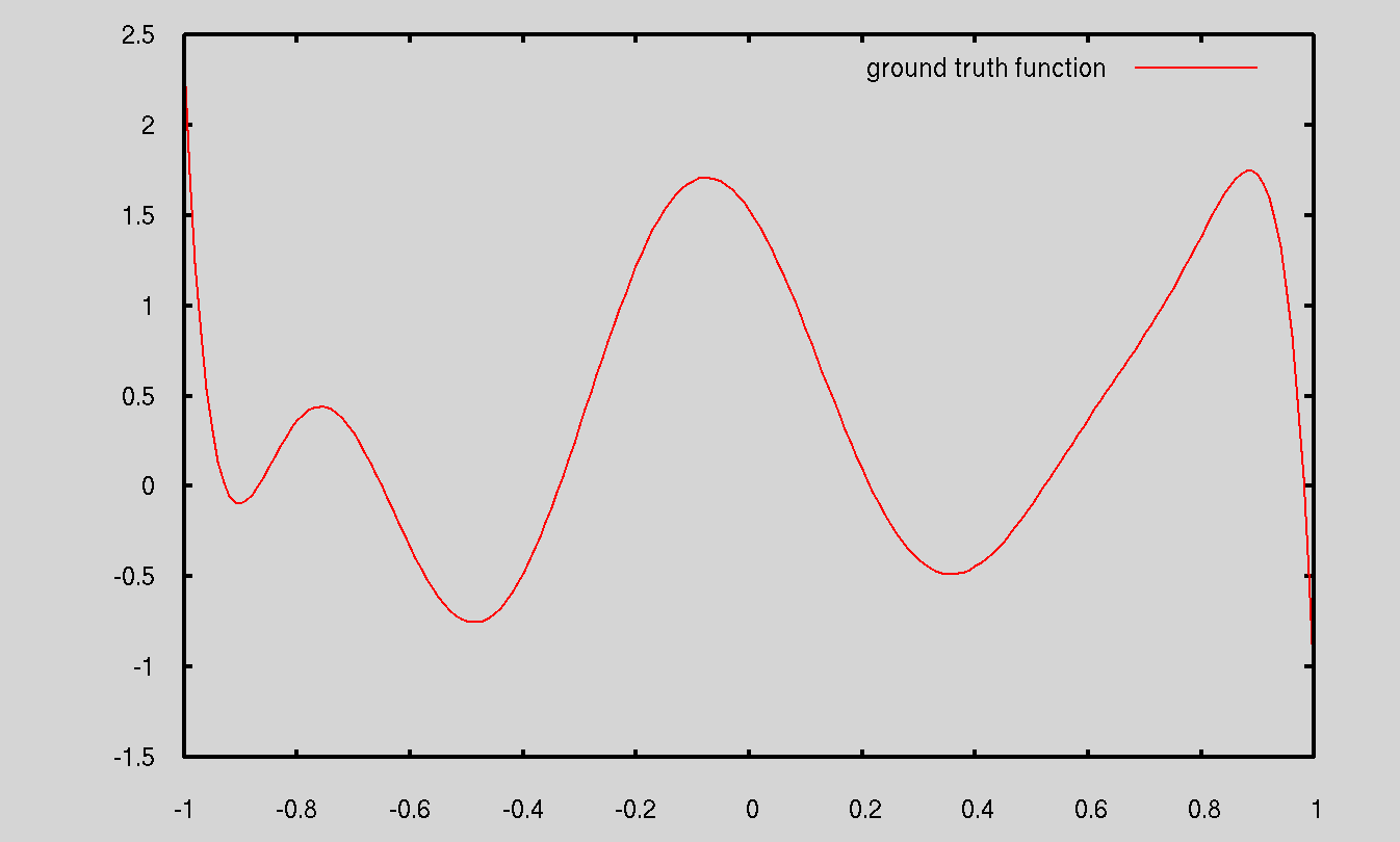
where $L_{i}(z)$ is the Legendre polynomial of degree $i$, and where the $w_{i}$ are independent Gaussian random variables $N(0,1)$. Thanks to the Legendre polynomials being orthogonal, this model produces random polynomials $f$ with a nice range; see an example in Fig. 1. Since we use Fourier features while $f$ is a polynomial (and non-periodic), there is no exact solution.

Figure 1: A ground truth function $f$ sampled from the model (19).

Equilibration was run for $50$ steps, as described in Section 5.1. We presented a random sequence of $1,000$ samples $(z,f(z))$ with uniform random $z\in[-1;1]$.

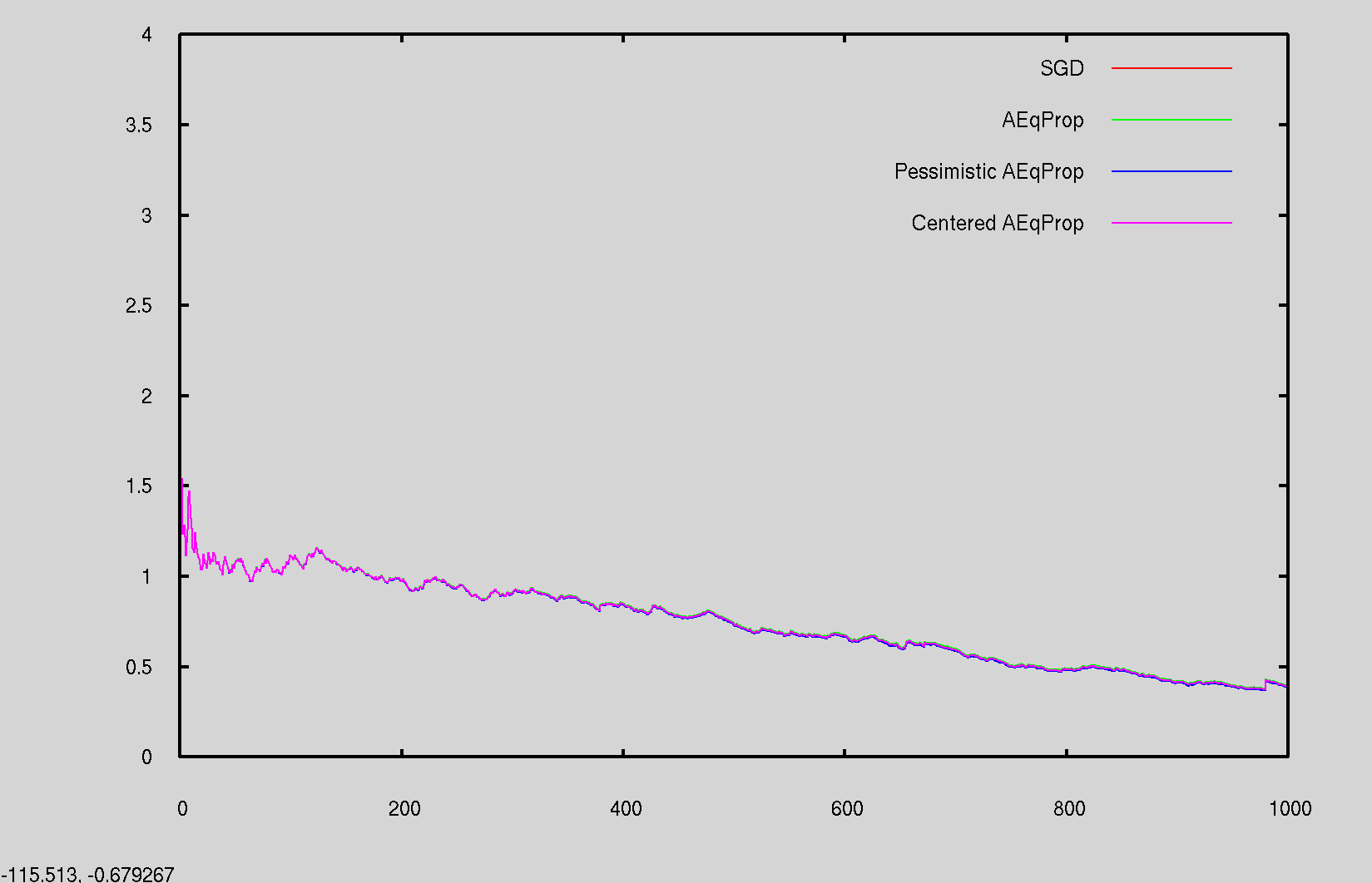
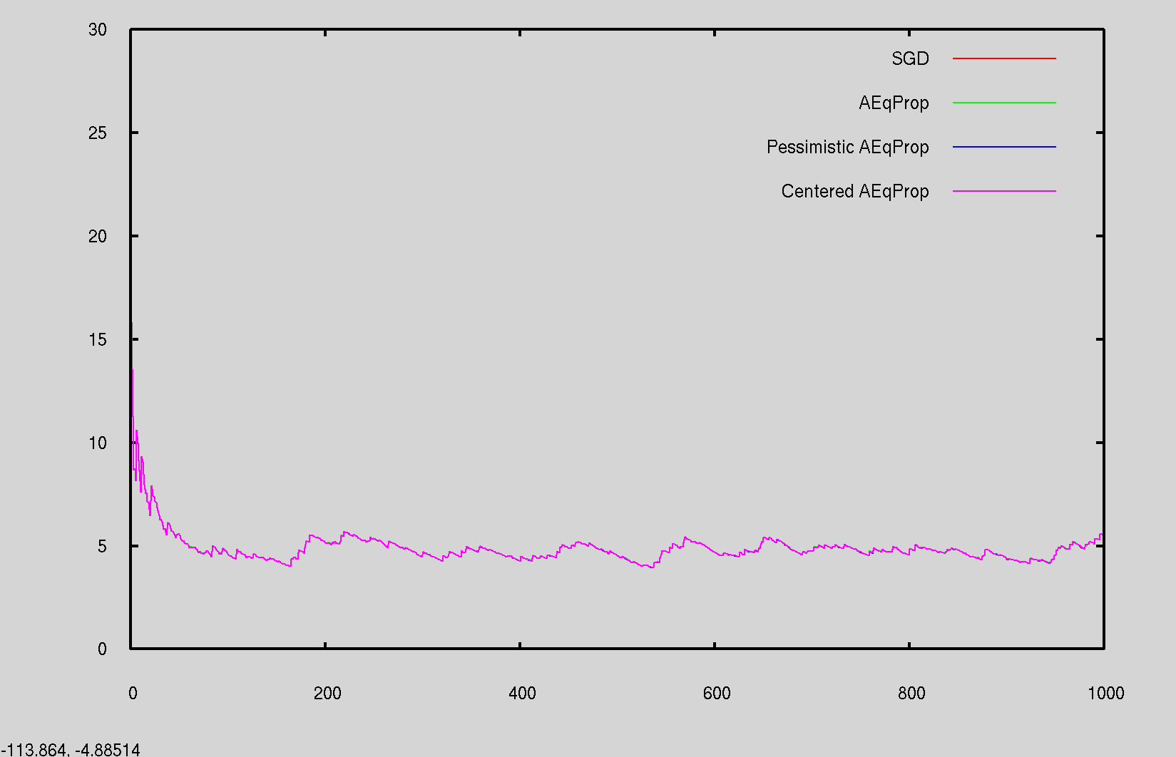
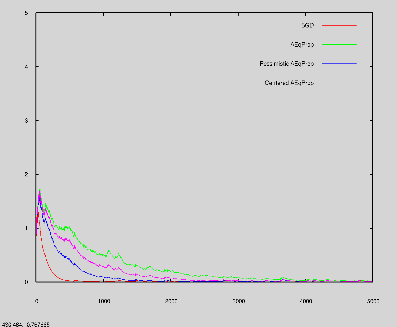
We tested values $\varepsilon,\beta\in\{0.5,0.1,0.01\}$, thus including relatively large and small values. We tested Æqprop, Pessimistic Æqprop, and Centered Æqprop. For reference we also compare to ordinary SGD with learning rate $\varepsilon\beta$, according to Theorem 1. The results are reported in Fig. 2.

For $\beta=0.01$, the curves are virtually indistinguishable. For $\beta=0.1$ there are some slight differences: Centered Æqprop is virtually indistinguishable from SGD, in accordance with theory, while Pessimistic Æqprop seems to have a slightly lower error, and Æqprop a slightly larger one.

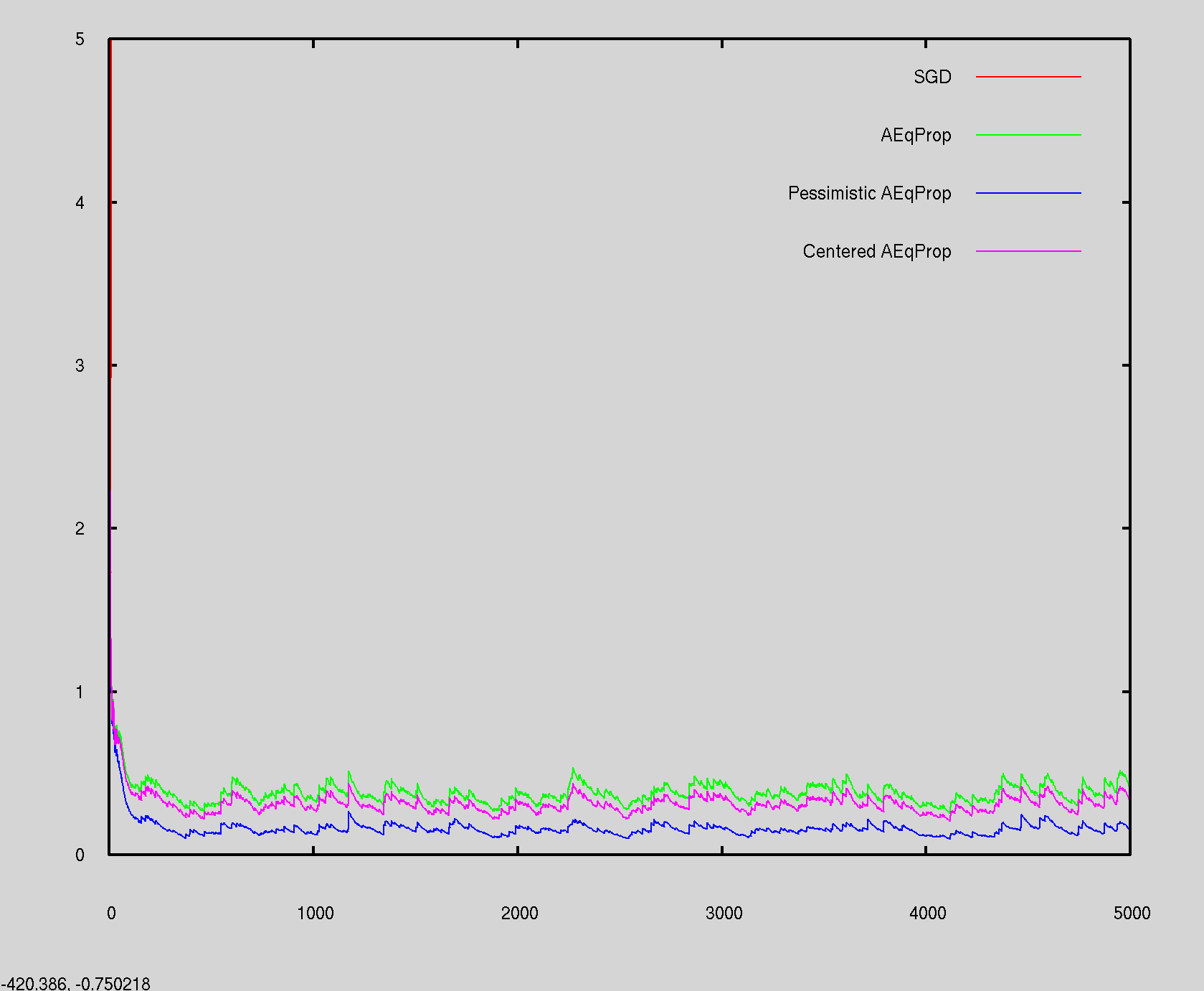
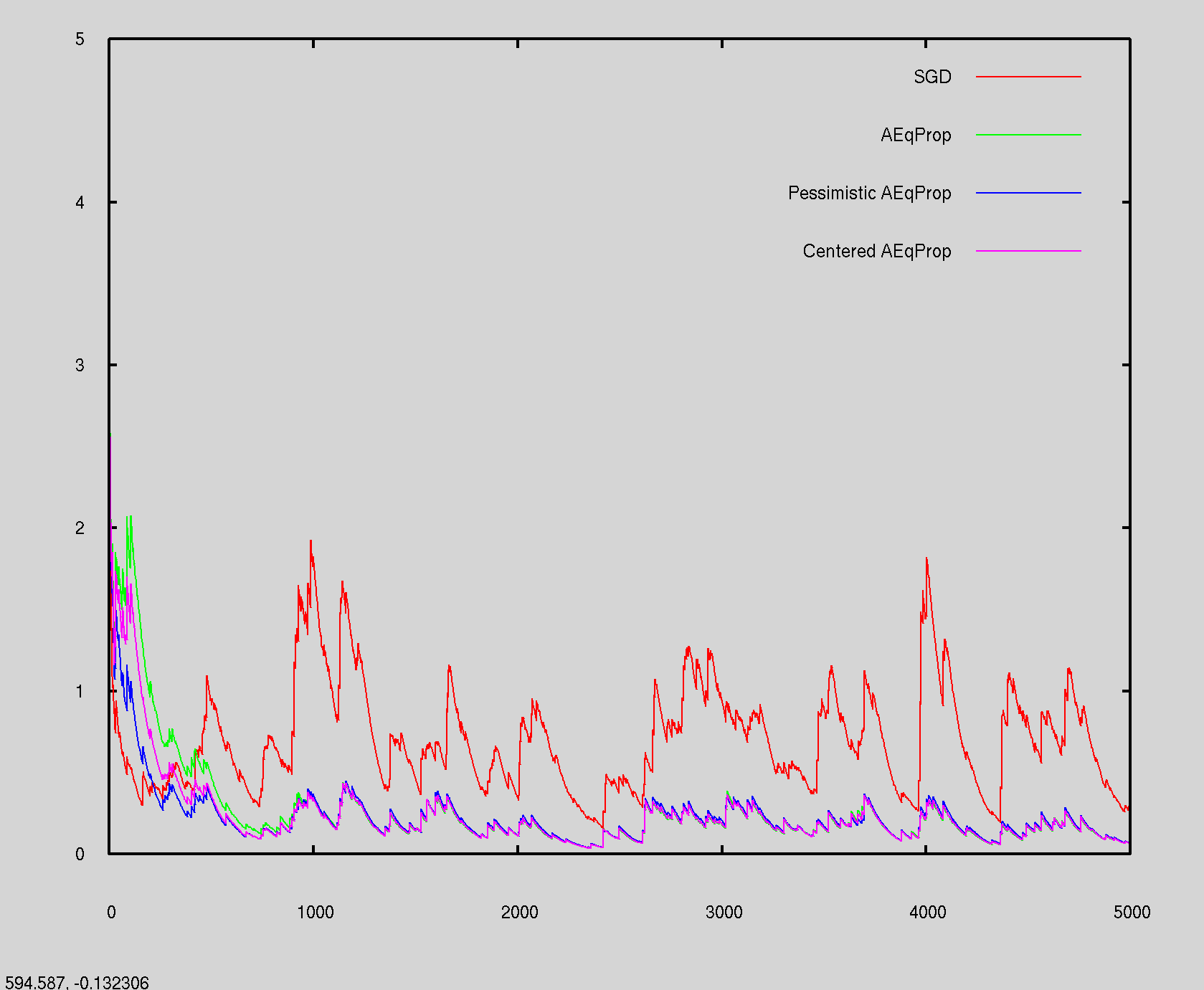
Results are more interesting with the more aggressive setting $\beta=.5$. Here, once more, Centered Æqprop stays very close to SGD, but the differences get more pronounced for the other variants. For small $\varepsilon$, Pessimistic Æqprop has the best performance while Æqprop is worse. However, when $\varepsilon$ gets larger, Pessimistic Æqprop becomes less numerically stable.

The most surprising result is with the most aggressive setting $\beta=.5$, $\varepsilon=.5$, corresponding to the largest learning rate $\varepsilon\beta$. With this setting, SGD gets unstable (the learning rate is too large), and so do Pessimistic Æqprop and Centered Æqprop. However, Æqprop optimizes well. So, in this experiment, Æqprop seems to be more stable than SGD and supports larger learning rates, with settings for $\beta$ and $\varepsilon$ that clearly do not have to be very small.

Figure 2: SGD, Æqprop, Pessimistic Æqprop, and Centered Æqprop on the linear regression problem for various values of $\beta$ and $\varepsilon$. Top row: $\beta=0.5$. Middle row: $\beta=0.1$. Bottom row: $\beta=0.01$. Left column: $\varepsilon=0.5$. Middle column: $\varepsilon=0.1$. Right column: $\varepsilon=0.01$.

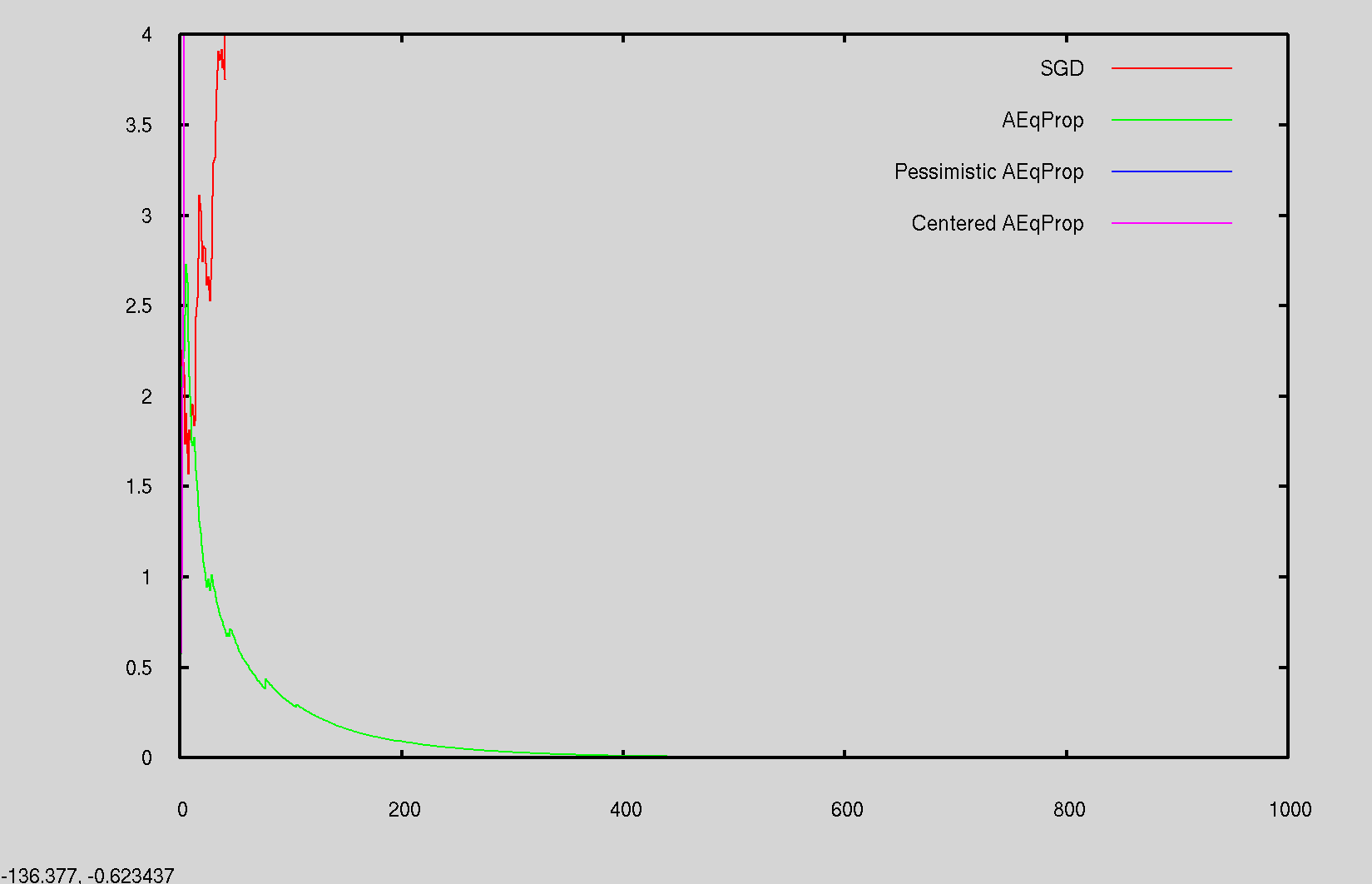
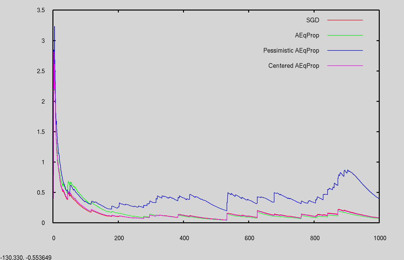
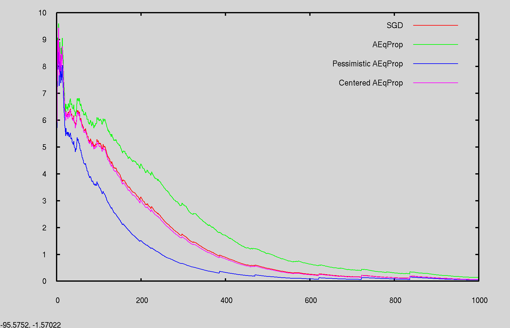
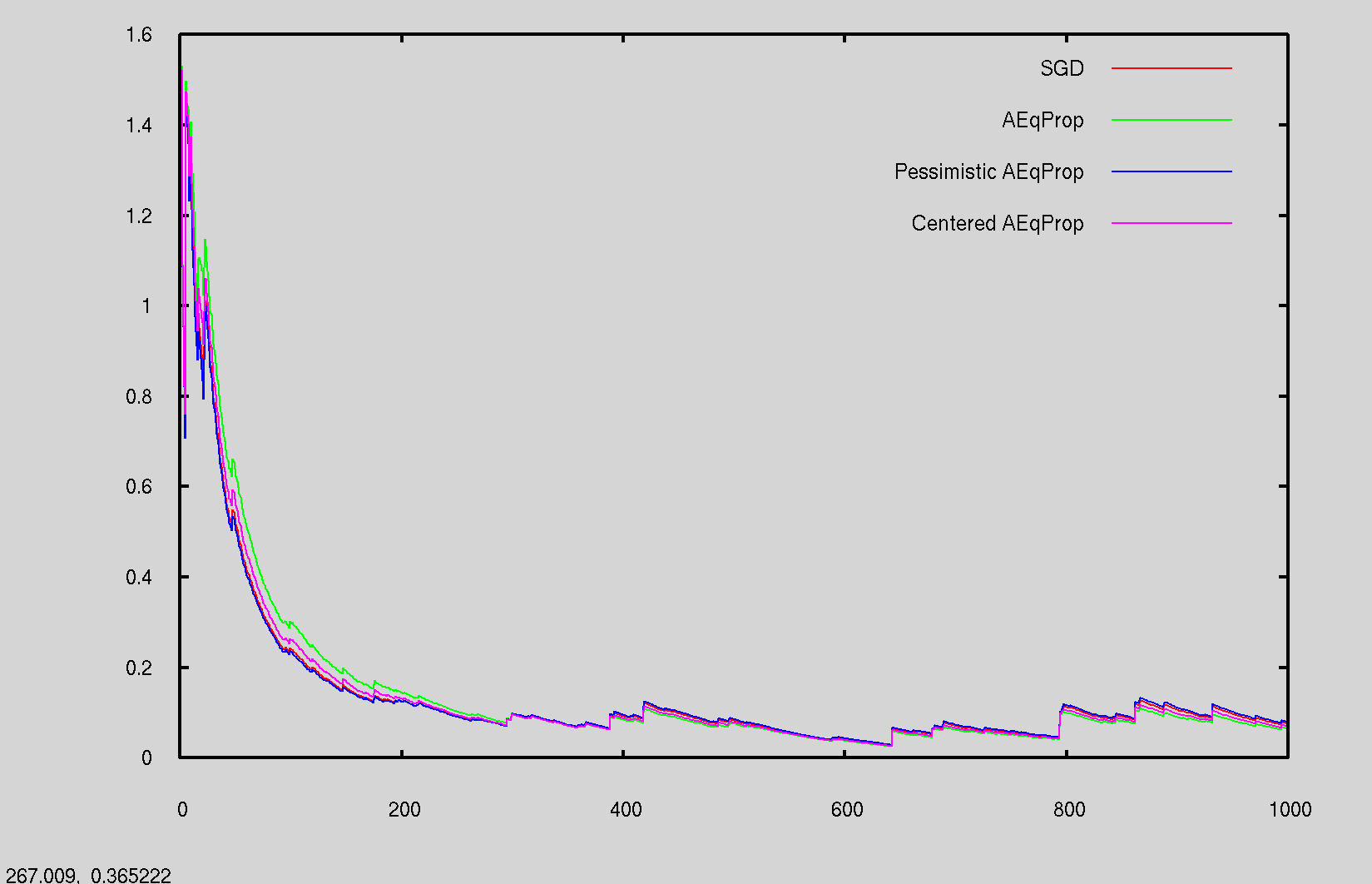
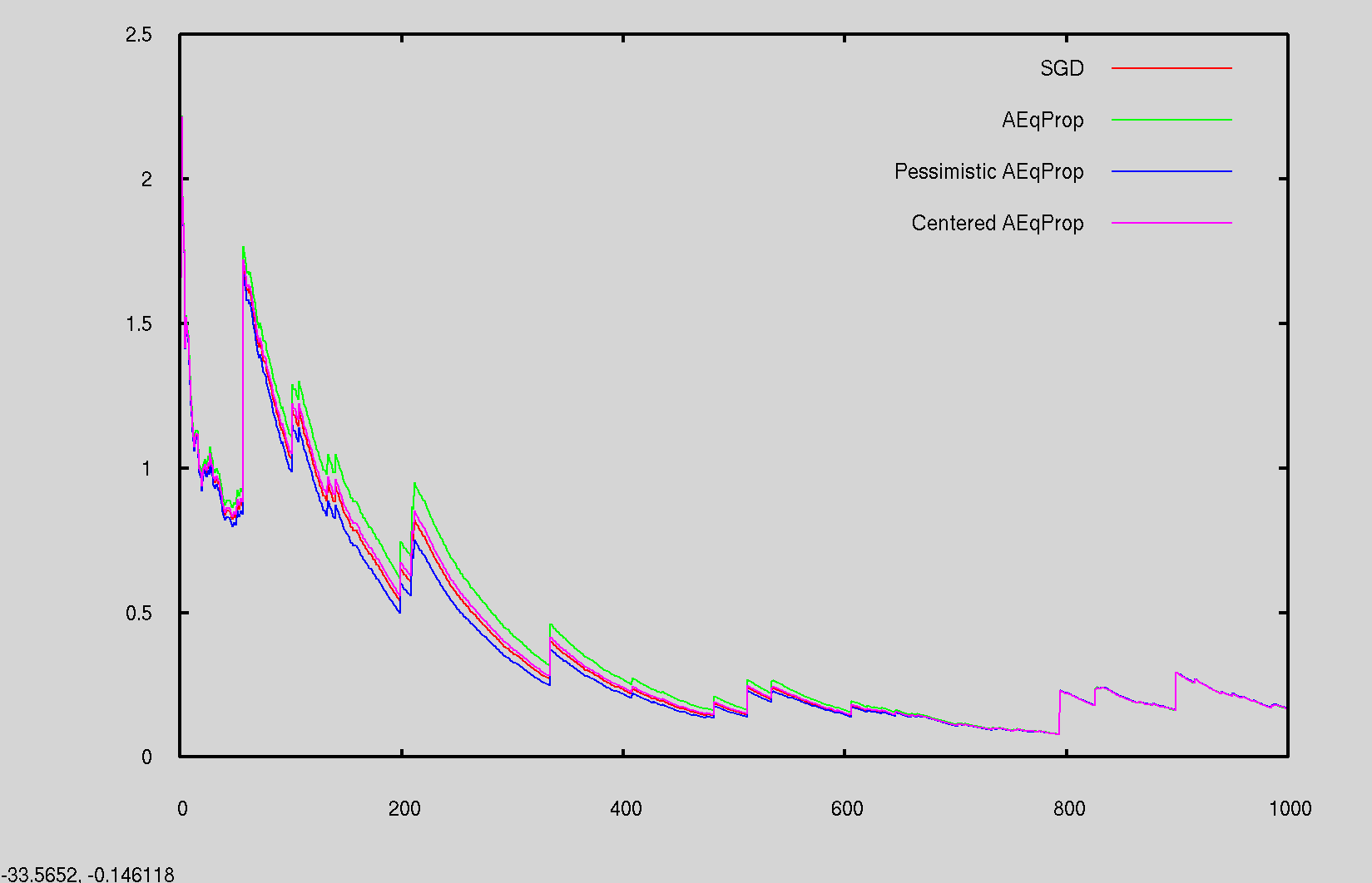
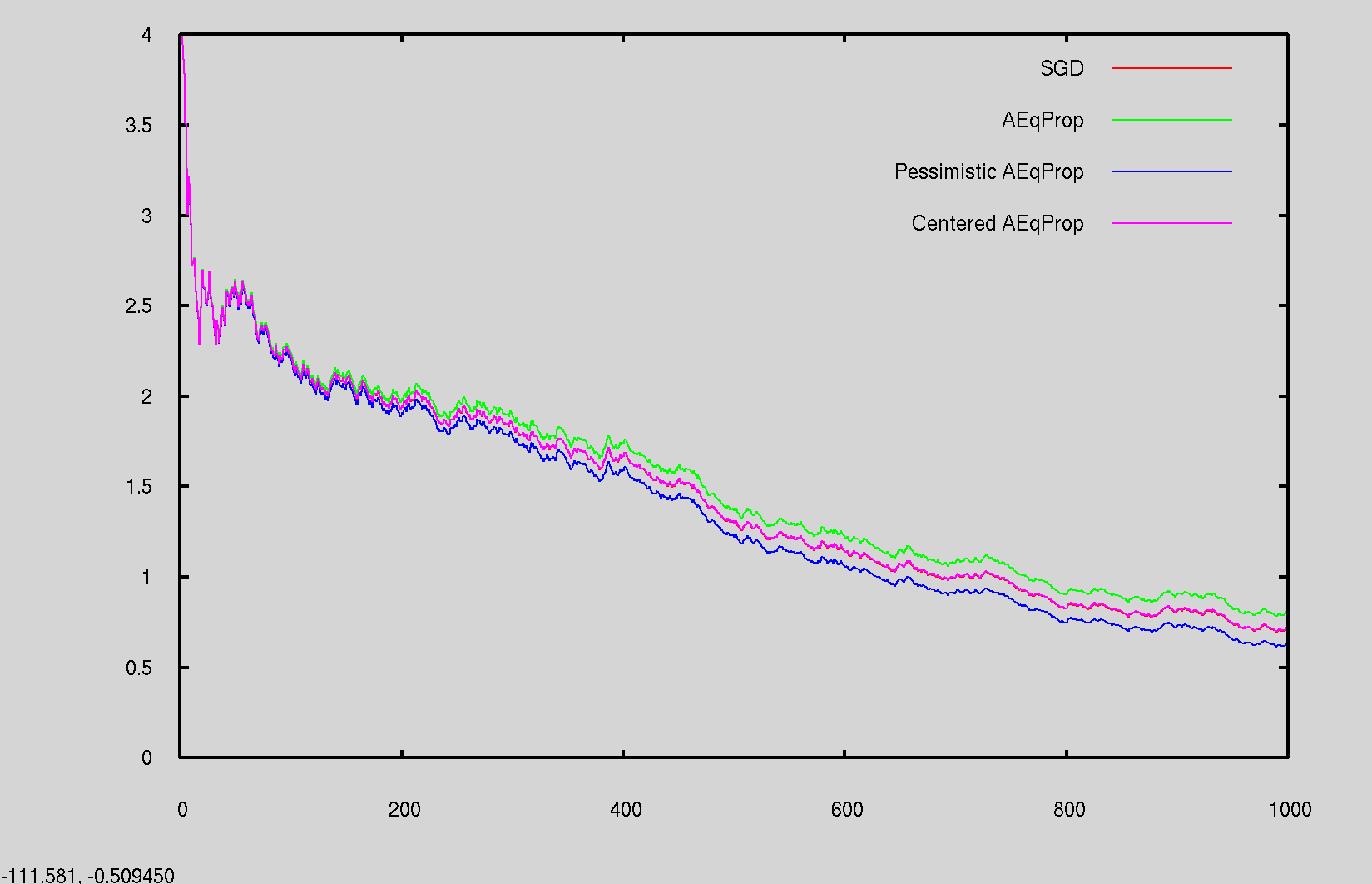
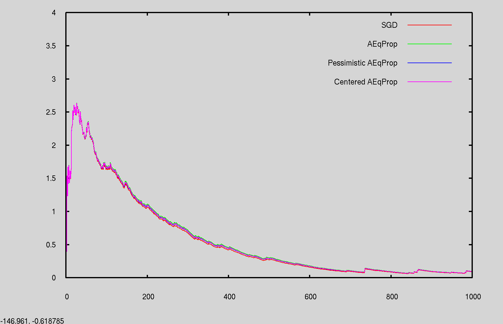
The numerical instability of Pessimistic and Centered Æqprop for large $\beta$ is due to the energy $-\beta C(s,y)$: since $C$ can tend to $\infty$, this energy is minimized when $C$ is infinite, with $s\to\infty$. This can be corrected simply by adding $\left\lVert s\right\rVert^{2}$ to the energy function $E$ of the system: then as long as $\beta<2$ the energy is bounded below and cannot diverge. This changes the prediction model, however, inducing a preference for smaller values of $s$.

This is tested in Fig. 3: with $\beta=1.5$, Pessimistic and Centered Æqprop are stable again, and all variants of Æqprop seem to work even in a regime where SGD itself is unstable (Fig. 3, left and middle). However, convergence seems to be slower (we used $5,000$ samples instead of $1,000$ in the figure). Once stabilized, it seems again that Pessimistic Æqprop tends to have smaller error than the other two variants.

Figure 3: SGD, Æqprop, Pessimistic Æqprop, and Centered Æqprop on the linear regression problem for $\beta=1.5$ and for $\varepsilon=0.5$ (left) $\varepsilon=0.1$ (middle), and $\varepsilon=0.01$ (right), with an added term $\left\lVert s\right\rVert^{2}$ to the energy function.

5.3 Hopfield-Like Networks and Real Datasets

Following the simulations of Scellier and Bengio (2017); Ernoult et al. (2019); Laborieux et al. (2021) with Eqprop, we test Æqprop on dense and convolutional Hopfield-like networks. We train the networks on MNIST and FashionMNIST.

Dense Hopfield-like network.

We consider the setting of classification. In a layered Hopfield network, the state variable is of the form $s=(s_{1},s_{2},\ldots,s_{N})$ where $s_{1},s_{2},\ldots,s_{N-1}$ are the ‘hidden layers’ and $s_{N}$ is the ‘output layer’. Denoting $s_{0}=x$ the inputs, the Hopfield energy function is

$$E(\theta,x,s)=\sum_{k=1}^{N}\frac{1}{2}\|s_{k}\|^{2}+\sum_{k=1}^{N}E_{k}^{\rm dense}(w_{k},s_{k-1},s_{k})-\sum_{k=1}^{N}b_{k}^{\top}s_{k},$$ (20)

where

$$E_{k}^{\rm dense}(w_{k},s_{k-1},s_{k}):=-s_{k}^{\top}w_{k}s_{k-1}$$ (21)

is the energy of a dense interaction between layers $k-1$ and $k$, parameterized by the $\dim(s_{k-1})\times\dim(s_{k})$ matrix $w_{k}$. The set of parameters of the model is $\theta=\{w_{k},b_{k}\mid 1\leq k\leq N\}$, where $w_{k}$ are the weights and $b_{k}$ the biases. We recall that the state of the model at equilibrium given an input $x$ is $s(\theta,x)=\underset{s\in\mathcal{S}}{\min}\;E(\theta,x,s)$, where $\mathcal{S}$ is the state space, i.e. the space of the state variables $s$. We choose $\mathcal{S}$ of the form $\mathcal{S}=\prod_{k=1}^{N}[p_{k},q_{k}]^{\dim(s_{k})}$, where $[p_{k},q_{k}]$ is a closed interval of $\mathbb{R}$ and $\dim(s_{k})$ is the number of units in layer $k$. This choice of $\mathcal{S}$ ensures that $s(\theta,x)$ is well defined (there exists a minimum for $E$ in $\mathcal{S}$) and also introduces nonlinearities: for fixed $\theta$, $s(\theta,x)$ is a nonlinear response of $x$.

Convolutional Hopfield-like interactions.

Convolutional layers can be incorporated to the network by replacing some of the dense interactions $E_{k}^{\rm dense}$ in the energy function by convolutional interactions:

$$E_{k}^{\rm conv}(w_{k},s_{k-1},s_{k}):=-s_{k}\bullet\mathcal{P}\left(w_{k}\star s_{k-1}\right).$$ (22)

In this expression, $w_{k}$ is the kernel (the weights), $\star$ is the convolution operation, $\mathcal{P}$ is the average pooling operation, and $\bullet$ is the scalar product for pairs of tensors with same dimension.

Cost function.

We use the squared error cost function $C(s,y)=\|s_{N}-y\|^{2}$, where $s_{N}$ is the output layer and $y$ is the one-hot code of the label (in the classification tasks studied here).

Energy minimization.

For our simulations, we require a numerical method to minimize the global energy with respect to the ‘floating variables’ ($s_{k}$, $w_{k}$ and $b_{k}$). For each variable $z\in\{s_{k},w_{k},b_{k}\mid 1\leq k\leq N\}$, we note that the global energy $\mathcal{E}$ is a quadratic function of $z$ given the state of other variables fixed. That is, the global energy as a function of $z$ is of the form $\mathcal{E}(z)=az^{2}+bz+c$, for some real-valued coefficients $a$, $b$ and $c$. The minimum of $\mathcal{E}(z)$ in $\mathbb{R}$ is obtained at $z=-b/2a$, and therefore, the minimum in the interval $[p_{k},q_{k}]$ is obtained at $z=\min(\max(p_{k},-b/2a),q_{k})$. We use this property to optimize $\mathcal{E}$ with the following strategy: at each step, we pick a variable $z$ and compute the state of $z$ that minimizes $\mathcal{E}$ given the state of other variables fixed. Then we pick another variable and we repeat. We repeat this procedure until convergence.

Homeostatic control.

To accelerate simulations, we use the following method to save computations in the first phase of training (homeostatic phase): first, we keep $\theta$ fixed to its current value and we calculate the state of the layers ($s_{1},s_{2},\ldots,s_{N}$) that minimizes the energy $E+\beta C$ for fixed $\theta$; then we calculate the value of the control knob $u$ for which the parameter $\theta$ is at equilibrium. Recalling that $\mathcal{E}=||u-\theta||^{2}/2\epsilon+E+\beta C$, this value of $u$ can be computed in one step as it is characterized by $\frac{\partial\mathcal{E}}{\partial\theta}=0$, i.e. $u=\theta+\epsilon\frac{\partial E}{\partial\theta}$, where $\frac{\partial E}{\partial\theta}$ is the partial derivative of $E$ wrt $\theta$ (not the total derivative). For instance, we have $\frac{\partial E}{\partial b_{k}}=-s_{k}$ for the bias $b_{k}$, and $\frac{\partial E}{\partial w_{k}}=\frac{\partial E_{k}^{\rm dense}}{\partial w_{k}}=-s_{k-1}s_{k}^{\top}$ for dense weight $w_{k}$.

MNIST and FashionMNIST.

We train a dense Hopfield-like network and a convolutional Hopfield-like network on MNIST and FashionMNIST. Both networks have an input layer of size $1\times 28\times 28$ and an output layer with $10$ units. In addition, the dense network has one hidden layer of $2048$ units, whereas the convolutional network has two hidden layers of size a $32\times 12\times 12$ and $64\times 4\times 4$ : the first two interactions ($x-s_{1}$ and $s_{1}-s_{2}$) are convolutional with kernel size $5\times 5$, zero padding, and average pooling; the last interaction ($s_{2}-s_{3}$) is dense.

Baseline.

Since Hopfield networks are defined by energy minimization, it is not possible to apply backpropagation directly as a baseline. Still, it is possible to compute gradients via the whole procedure used to find the approximate energy minimizer: unfold the whole graph of computations during the free phase minimization (with $\beta=0$), and compute the gradient of the final loss with respect to the parameters. Then, take one step of gradient descent for each parameter $\theta_{k}$, with step size $\beta\varepsilon_{k}$. This is the baseline denoted as autodiff in the table.

However, the autodiff procedure seems to be numerically unstable, for reasons we have not identified.

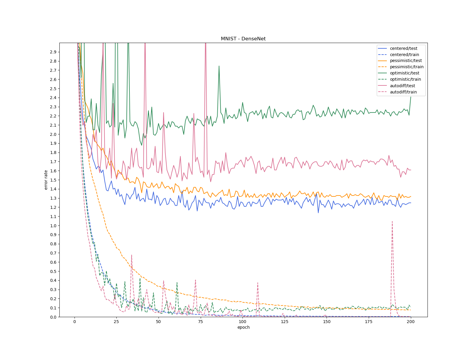
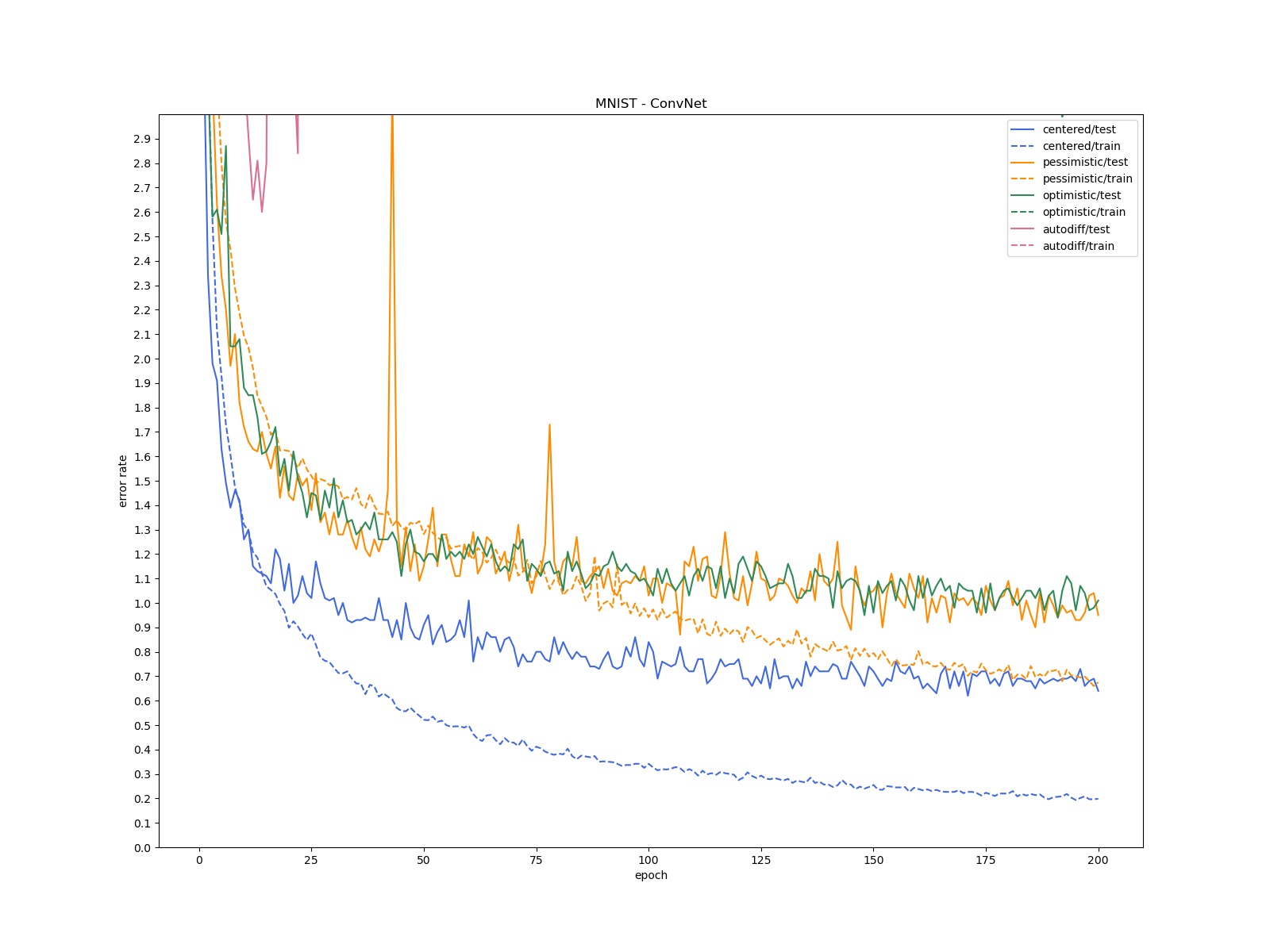
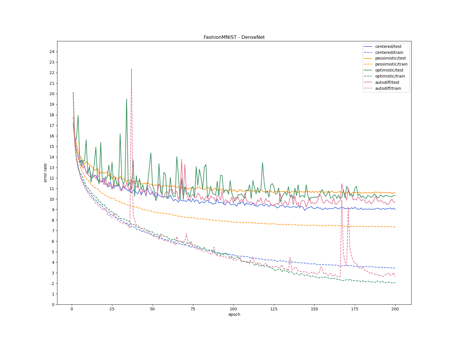
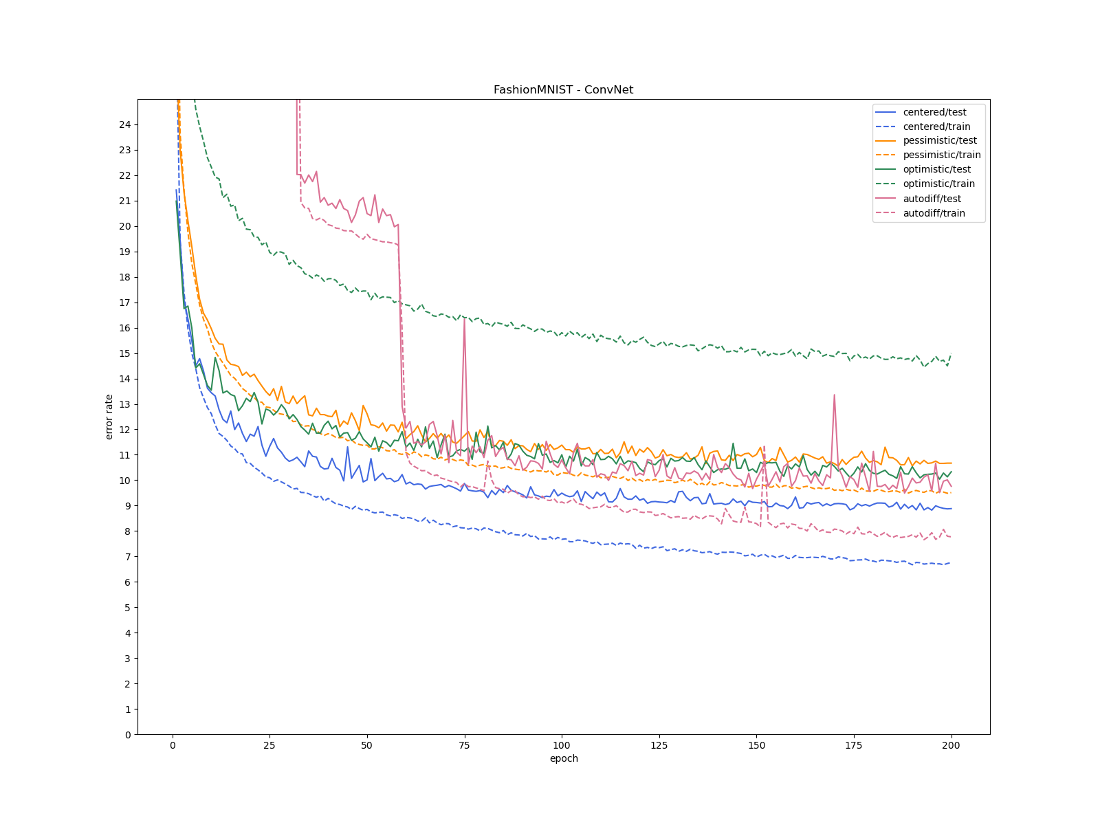
The results are reported in Table 1, and show that Æqprop successfully manages to learn on these datasets, even with the relatively large $\beta$ used ($0.5$ for dense networks and $0.2$ for convolution-like networks). Centered Æqprop seems to offer the best precision.

Table 1: Simulation results on MNIST and FashionMNIST. We train dense networks and convolutional Hopfield-like networks. For each experiment, we perform five runs of 200 epochs. For each run we compute the mean test error rate and the mean train error rate over the last 50 epochs. We then report the mean and standard deviation over the 5 runs. Implementation details are provided in Appendix C.

			Error (%)
Task	Network	Training Method	Test	(Train)
MNIST	Dense Hopfield-like	Optimistic Æqprop	$2.36\pm 0.07$	($0.10$)
		Pessimistic Æqprop	$1.38\pm 0.03$	($0.09$)
		Centered Æqprop	$\bf{1.29\pm 0.04}$	($0.00$)
		Autodiff	$72.37\pm 35.35$	($71.96$)
	Convolutional Hopfield-like	Optimistic Æqprop	$1.12\pm 0.07$	($3.62$)
		Pessimistic Æqprop	$1.11\pm 0.08$	($1.73$)
		Centered Æqprop	$\bf{0.76\pm 0.05}$	($0.24$)
		Autodiff	$89.63\pm 0.96$	($89.61$)
FashionMNIST	Dense Hopfield-like	Optimistic Æqprop	$10.53\pm 0.12$	($2.30$)
		Pessimistic Æqprop	$10.73\pm 0.07$	($7.46$)
		Centered Æqprop	$\bf{9.28\pm 0.10}$	($3.69$)
		Autodiff	$10.18\pm 0.32$	($4.25$)
	Convolutional Hopfield-like	Optimistic Æqprop	$10.69\pm 0.17$	($15.11$)
		Pessimistic Æqprop	$11.16\pm 0.20$	($9.89$)
		Centered Æqprop	$\bf{9.17\pm 0.19}$	($7.00$)
		Autodiff	$29.55\pm 30.47$	($28.27$)

6 Related Work

There is a considerable amount of literature on the design of fast and energy-efficient learning systems. While some aim to improve the digital hardware for running and training existing deep learning algorithms, others focus on designing novel algorithms for neural network training and inference on new energy-efficient hardware. We can differentiate this literature according to the presence or not of an explicit model of the physical computation performed.

Explicit approaches.

A first approach is to improve the hardware for running neural networks and training them via backpropagation. For instance, Courbariaux et al. (2015) explore the use of specialized digital processors for low-precision tensor multiplications, whereas Ambrogio et al. (2018); Xia and Yang (2019) investigate the use of crossbar arrays to perform matrix-vector multiplications in analog. However, given the mismatches in analog devices, the latter approach requires mixed digital/analog hardware. These approaches can be classified as explicit, as the state of the underlying system can be expressed as $s=f(\theta,x)$ where $f=f_{N}\circ\ldots\circ f_{2}\circ f_{1}$ is the composition of (elementary) functions defined by analytical formulae.

Physics-aware training (Wright et al., 2022) is a hybrid physical-digital approach in which inference is carried out on an energy-efficient physical device, but parameter training is done using gradients computed from an explicit digital model of the physical device. This is demonstrated on machine learning tasks using various examples of physical realizations (optical, mechanical, electronic).

Spiking neural networks (SNNs) are networks of individual units that communicate through low-energy electrical pulses, mimicking the spikes of biological neurons (Zenke et al., 2021). Most SNN models are explicit, and are confronted to the problem of ‘differentiation through spikes’, which arises when using the chain rule of differentiation to compute the gradients of the loss. However, the implicit Eqprop framework has also been used to train SNNs (Mesnard et al., 2016; O’Connor et al., 2019; Martin et al., 2021).

Implicit approaches.

In contrast, implicit approaches aim to harness the underlying physical laws of the device for training and inference. These laws are seldom in the form of explicit analytical formulae; rather, they are often characterized by the minimization of an energy function. For instance, the equilibrium state of an electrical circuit composed of nonlinear resistors (such as diodes) is given by the minimization of the so-called co-content (Millar, 1951), a nonlinear analogue of electrical power.

Equilibrium propagation (Eqprop) was designed to train neural networks in this setting (Scellier and Bengio, 2017). First formulated in the context of Hopfield networks, Eqprop has then been deployed in the context of nonlinear resistive networks and other physical systems (Kendall et al., 2020; Scellier, 2021). The feasibility of Eqprop training has been further demonstrated empirically on a small resistive circuit (Dillavou et al., 2021). A ‘centered’ version of Eqprop was also proposed and tested numerically (Laborieux et al., 2021).

Stern et al. (2021) propose a variant of Eqprop called coupled learning. In the second phase, rather than nudging the output unit by adding an energy term $\beta C$ to the system, the output unit is clamped to $\beta y+(1-\beta)y_{0}$, where $y_{0}$ is the output unit’s equilibrium state without nudging (i.e. the ‘prediction’) and $y$ is the desired output.

Yet, as mentioned in Section 1 (see also Appendix D for more details), Eqprop as well as the variant of Stern et al. (2021) require explicit knowledge of the underlying energy function, storage of the equilibrium state of the first phase, and additional mechanisms for updating the parameters. Æqprop overcomes all these three limiting factors.

The second of these three issues is considered in another variant of Eqprop, Continual Eqprop (CEP) (Ernoult et al., 2020): the parameters are updated continually in the second phase of training to avoid storing the first equilibrium state. However, the dynamics of the parameters in CEP is chosen ad hoc: no physical mechanism is proposed to account for the specific dynamics of the parameters. Anisetti et al. (2022) propose a different solution to the problem of storing the first equilibrium state in Eqprop: in the second phase, another physical quantity (e.g. the concentration of a chemical) is used to play the role of error signals.

7 Discussion, Limitations, and Conclusion

In this paper, we have proposed Agnostic equilibrium propagation (Æqprop), a novel algorithm by which physical systems can perform stochastic gradient descent without explicitly computing gradients. Æqprop leverages energy minimization, homeostatic control and nudging towards the desired output to obtain an accurate estimate of the result of a gradient descent step (Theorem 1). Although it builds upon equilibrium propagation (Eqprop) (Scellier and Bengio, 2017), Æqprop distinguishes itself from Eqprop in the following ways; i) it does not require any explicit knowlegde of the analytical form of the underlying energy function, ii) the equilibrium state at the end of the first phase is not needed to be stored and iii) the parameter update at the end of a gradient step is performed automatically in Æqprop and no additional mechanism needs to be introduced to perform this update. Thus, Æqprop mitigates major limitations of Eqprop (and its variants) and, in principle, significantly increases the range of hardware on which statistical learning can be performed.

In addition to showing that Æqprop estimates gradient descent steps accurately, we have also derived a Lyapunov function for Æqprop and proved that this Lyapunov function improves monotonically along the Æqprop trajectory, suggesting enhanced robustness of this algorithm with non-infinitesimal step sizes, compared to standard SGD. Moreover, we consider different variants of Æqprop (optimistic, pessimistic and centered), each with desirable properties. In particular, the pessimistic version of Æqprop optimizes an upper bound of the true loss function whereas the centered version provides a better (second-order) approximation of the loss. We also illustrated Æqprop (and its variants) numerically with a simple linear regression example as well as with Hopfield-like networks on the MNIST and FashionMNIST datasets, showing that Æqprop successfully implements gradient descent learning in practice.

At this stage, it is germane to examine the main assumptions on which Æqprop rests. Clearly, a large number of physical systems are based on energy minimization and can be used in the context of Æqprop, as they have already been for Eqprop. Nudging towards a desired output is a key design principle of Æqprop as well as Eqprop. Such nudging has been realized on model physical systems such as in Dillavou et al. (2021) and references therein, and such devices can, in principle, be used in the context of Æqprop as well. Next, our technical assumptions require the existence and smoothness of local minimizers of the energy function. Uniqueness of the minimizer is not required, but then, the system should remain around one of its possible modes for the duration of training; training will be perturbed if the system jumps to another minimizer.

Homeostatic control of the parameters is a limiting assumption for Æqprop. In this context, we would like to point that there is quite a bit of flexibility in terms of the form of the coupling energy $U$. It need not be quadratic: an arbitrary form of $U$ leads to a Riemannian instead of Eucliean gradient descent step, still decreasing the Lyapunov error function. Similarly, the coupling parameter $\varepsilon$ need not be infinitesimal: relatively large values of $\varepsilon$ (weak coupling) are allowed. In the end, it is hard to imagine a way to train parameters without some means of monitoring and controlling them. In Æqprop this control only takes the form of being able to maintain stasis of the current parameters by adjusting some control knobs. Æqprop offers one way to build gradient descent from such a generic control mechanism.

Finally, the existence of Æqprop has a more general interest, in showing that generic, physically plausible ingredients such as homeostatic control and output nudging are enough, in principle, for natural (bio)physical systems to exhibit genuine gradient descent learning.

Appendix A A Generalization of Theorem 1: Æqprop with Large $\varepsilon$ or $\beta$, Centered and Pessimistic Æqprop

We now extend Theorems 1 and 2 in the following directions:

• Variants such as Pessimistic Æqprop and Centered Æqprop (Section 4) are covered.

• Only one of $\varepsilon$ or $\beta$ needs to tend to $0$.

• The control energy $U(u,\theta)$ is not necessarily the quadratic $\left\lVert u-\theta\right\rVert^{2}/2$.

So at each instant, we set input knobs $x$, control knobs $u$, and possibly (if $\beta>0$) a desired output $y$, and assume that the system reaches an equilibrium $(\theta_{\star},s_{\star})=\operatorname*{arg\,min}_{(\theta,s)}\;\mathcal{E}(u,\theta,s,x,y,\varepsilon,\beta)$, where

$$\mathcal{E}(u,\theta,s,x,y,\varepsilon,\beta):=U(u,\theta)/\varepsilon+E(\theta,x,s)+\beta C(s,y)$$ (23)

is the global energy function of the system. (Assumption 6 in Appendix B ensures the argmin is well-defined.)

Then we follow the Æqprop procedure from Section 2. To cover variants like Pessimistic and Centered Æqprop, here we use two values $\beta_{1}<\beta_{2}$ in the two phases of the algorithm. Namely, we first set a control value $u_{t}$ such that the equilibrium value $\theta_{t-1}$ does not change when we introduce the new input $x_{t}$, the desired output $y_{t}$ and nudging $\beta_{1}$. Then we obtain the next parameter by changing the nudging to $\beta_{2}$ and letting the system reach equilibrium.

This time, we define the Lyapunov function

$$\mathcal{L}_{\beta_{1};\beta_{2}}(\theta,x,y)\mathrel{\mathop{:}}=\frac{1}{\beta_{2}-\beta_{1}}\int_{\beta^{\prime}=\beta_{1}}^{\beta_{2}}C(s_{\beta^{\prime}}(\theta,x,y),y)\operatorname{d}\!{}\beta^{\prime}$$ (24)

where as before,

$$s_{\beta}(\theta,x,y)\mathrel{\mathop{:}}=\operatorname*{arg\,min}_{s}\{E(\theta,x,s)+\beta C(s,y)\}.$$ (25)

This Lyapunov function tends to the loss

$$\mathcal{L}(\theta,x,y)\mathrel{\mathop{:}}=C(s(\theta,x),y)$$ (26)

when $\beta_{1}$ and $\beta_{2}$ tend to $0$, where $s(\theta,x)\mathrel{\mathop{:}}=\operatorname*{arg\,min}_{s}E(\theta,x,s)=s_{0}(\theta,x,y)$ by definition.

The next theorem states that Æqprop performs a step of Riemannian stochastic gradient descent for the input-output pair $(x_{t},y_{t})$, with step size (learning rate) $\varepsilon(\beta_{2}-\beta_{1})$, loss function $\mathcal{L}_{\beta_{1};\beta_{2}}$, and preconditioning matrix (Riemannian metric) $M$. When $\beta_{1}$ and $\beta_{2}$ both tend to $0$, the Lyapunov function $\mathcal{L}_{\beta_{1};\beta_{2}}(\theta_{t-1},x_{t},y_{t})$ tends to the loss $\mathcal{L}(\theta_{t-1},x_{t},y_{t})$, thus recovering (Riemannian) stochastic gradient descent with the ordinary loss function. This theorem gives a better description of the behavior of Æqprop when $\beta_{1}$ and $\beta_{2}$ are not $0$: it still follows the (Riemannian) gradient descent of the closely related function $\mathcal{L}_{\beta_{1};\beta_{2}}$.

Theorem 3.

Let $\theta_{t-1}$ be some parameter value. Let $\beta_{1}<\beta_{2}$. Let $x_{t}$ and $y_{t}$ be some input and output value. Let $u_{t}$ be a control value such that

$$\theta_{t-1}=\operatorname*{arg\,min}_{\theta}\;\min_{s}\;\mathcal{E}(u_{t},\theta,s,x_{t},y_{t},\varepsilon,\beta_{1})$$ (27)

and let

$$\theta_{t}=\operatorname*{arg\,min}_{\theta}\;\min_{s}\;\mathcal{E}(u_{t},\theta,s,x_{t},y_{t},\varepsilon,\beta_{2})$$ (28)

working under the technical assumptions of Section B.2.

Then, for any $\varepsilon>0$ and $\beta_{2}>\beta_{1}$ (not necessarily tending to $0$) we have the Lyapunov property

$$\mathcal{L}_{\beta_{1};\beta_{2}}(\theta_{t},x_{t},y_{t})\leq\mathcal{L}_{\beta_{1};\beta_{2}}(\theta_{t-1},x_{t},y_{t}).$$ (29)

Moreover, when either $\varepsilon$, or $\beta_{2}-\beta_{1}$, or both, tend to $0$, we have

$$\theta_{t}=\theta_{t-1}-\varepsilon(\beta_{2}-\beta_{1})\,M^{-1}\partial_{\theta}\mathcal{L}_{\beta_{1};\beta_{2}}(\theta_{t-1},x_{t},y_{t})+O(\varepsilon^{2}(\beta_{2}-\beta_{1})^{2})$$ (30)

where $\mathcal{L}_{\beta_{1};\beta_{2}}$ is the Lyapunov function (24), and where $M$ is the positive definite matrix

$$M=M_{\beta_{1}}^{\varepsilon}(\theta_{t-1},x_{t},y_{t}) \mathrel{\mathop{:}}=\varepsilon\,\partial^{2}_{\theta}\left[\min_{s}\mathcal{E}(u_{t},\theta_{t-1},s,x_{t},y_{t},\varepsilon,\beta_{1})\right]$$ (31)

$$=\partial^{2}_{\theta}\left[U(u_{t},\theta_{t-1})+\varepsilon\,\min_{s}\{E(\theta_{t-1},x_{t},s)+\beta_{1}C(s,y_{t})\}\right]$$ (32)

When $\varepsilon\to 0$ we have $M=\partial^{2}_{\theta}U(u_{t}^{0},\theta_{t-1})+O(\varepsilon)$ where $u_{t}^{0}$ is such that $\theta_{t-1}=\operatorname*{arg\,min}_{\theta}U(u_{t}^{0},\theta)$. In particular, if $U(u,\theta)=\left\lVert u-\theta\right\rVert^{2}/2$ then $M=\operatorname{Id}+O(\varepsilon)$.

Finally, the Lyapunov function enjoys the following properties. For any $\beta_{1}<0<\beta_{2}$, we have

$$\mathcal{L}_{0;\beta_{2}}(\theta,x,y)\leq C(s(\theta,x),y)\leq\mathcal{L}_{\beta_{1};0}(\theta,x,y).$$ (33)

In particular, Pessimistic Æqprop optimizes an upper bound of the loss function. Moreover, when $\beta_{1}$ and $\beta_{2}$ tend to $0$ we have

$$\mathcal{L}_{\beta_{1};\beta_{2}}(\theta,x,y)=C(s(\theta,x),y)+O(\left\lvert\beta_{1}\right\rvert+\left\lvert\beta_{2}\right\rvert),$$ (34)

and if $\beta_{2}=-\beta_{1}=\beta/2$ (Centered Æqprop),

$$\mathcal{L}_{-\beta/2;\beta/2}(\theta,x,y)=C(s(\theta,x),y)+O(\beta^{2}).$$ (35)

When $\varepsilon\to 0$, the Riemannian metric $M$ tends to $\partial^{2}_{\theta}U(u_{t},\theta_{t-1})$, thus recovering ordinary gradient descent for quadratic $U$. Note that the Hessian $M$ is always nonnegative definite, because $\theta_{t-1}$ minimizes the function $\theta\mapsto\min_{s}\mathcal{E}(u_{t},\theta,s,x_{t},y_{t},\varepsilon,\beta_{1})$ by definition (27). Under the technical assumptions below, it is actually positive definite, so that $M^{-1}$ is well-defined.

For fixed, nonzero $\varepsilon$, the metric $M$ depends on $\theta_{t-1}$, on the input $x_{t}$, and also on $y_{t}$ if $\beta_{1}\neq 0$. Indeed, $E$ depends on $x_{t}$ in the definition of $G$, and $u_{t}$ itself depends on $x_{t}$ via (27). This dependency is at first order in $\varepsilon$.

Thus, for large $\varepsilon$, Æqprop produces a gradient descent with a sample-dependent preconditioning matrix. Since this preconditioning may be correlated with the gradient of the loss for sample $x_{t}$, this breaks the property of expected gradients in stochastic gradient descent, and may introduce bias. This bias disappears when $\varepsilon\to 0$: it is only a term $O(\varepsilon^{2}\beta)$ in (30).

Appendix B Proofs

In this section, we prove Theorem 1, Theorem 2 and Theorem 3. We proceed as follows:

• In Section B.1, we introduce the notation.

• In Section B.2, we state Definition 5 and Assumption 6, which gather the precise technical assumptions for the theorems, such as existence of the minima involved. Proposition 7 gives a simple sufficient condition for these assumptions to hold.

• In Section B.3, we establish important formulae relating the loss and Lyapunov function to the energy with a free-floating state (Theorem 8). We also prove the properties of the Lyapunov function stated in Theorem 3 (Proposition 9 and Corollary 11).

• In Section B.4, we prove the Lyapunov property of Theorem 2 using Theorem 8.

• In Section B.5, we prove a technical lemma (Lemma 12), under the assumptions of Assumption 6.

• In Section B.6, using Lemma 12 and Theorem 8, we prove the Riemannian SGD property of Theorem 3.

• In Section B.7, we prove Theorem 1 (the SGD property) as a corollary of Theorem 3, using Theorem 8 again.

B.1 Notation

Theorems 1 and 2 are particular cases of Theorem 3.

Since Theorem 3 deals with a fixed input-output pair $(x_{t},y_{t})$, in all proofs we assume that $x_{t}$ and $y_{t}$ are fixed, and omit them from the notation all along.

We denote

$$s_{\beta}(\theta)\mathrel{\mathop{:}}=\underset{s}{\arg\min}\{E(\theta,s)+\beta\,C(s)\}$$ (36)

the equilibrium state with nudging $\beta$ and

$$F(\beta,\theta)\mathrel{\mathop{:}}= \;\underset{s}{\min}\;\{E(\theta,s)+\beta\,C(s)\}$$ (37)

$$= \;E(\theta,s_{\beta}(\theta))+\beta C(s_{\beta}(\theta))$$ (38)

the minimal energy when $s$ is floating. The loss to optimize is

$$\mathcal{L}(\theta)\mathrel{\mathop{:}}=C(s_{0}(\theta)),$$ (39)

where $s_{0}(\theta)$ is the equilibrium state without nudging. For every $\beta_{1}<\beta_{2}$, the Lyapunov function is

$$\mathcal{L}_{\beta_{1};\beta_{2}}\left(\theta\right)\mathrel{\mathop{:}}=\frac{1}{\beta_{2}-\beta_{1}}\int_{\beta_{1}}^{\beta_{2}}C(s_{\beta}(\theta))\,d\beta.$$ (40)

We then introduce a control variable $u$ and we further augment the energy of the system by adding a coupling energy $U(u,\theta)/\varepsilon$ between $u$ and $\theta$, scaled by a positive scalar $\varepsilon$. We denote $G_{\beta}^{\varepsilon}(u,\theta)$ the global energy (23) minimized by the system (when $s$ is floating), rescaled by $\varepsilon$:

$$G_{\beta}^{\varepsilon}(u,\theta) \mathrel{\mathop{:}}=U(u,\theta)+\varepsilon\,F(\beta,\theta)$$ (41)

$$=U(u,\theta)+\varepsilon\,E(\theta,s_{\beta}(\theta))+\varepsilon\beta\,C(s_{\beta}(\theta)).$$ (42)

since the state that realizes the minimum of $F$ is $s_{\beta}(\theta)$.

Let $\theta_{\beta}^{\varepsilon}(u)$ be the equilibrium parameter, i.e. the minimizer of the global energy:

$$\theta_{\beta}^{\varepsilon}(u)\mathrel{\mathop{:}}=\underset{\theta}{\arg\min}\;G_{\beta}^{\varepsilon}(u,\theta).$$ (43)

Given a parameter value $\theta$, we denote $u=u_{\beta}^{\varepsilon}(\theta)$ the value of the control knobs such that $\theta$ is at equilibrium given $\beta$ and $\varepsilon$, i.e.

$$u=u_{\beta}^{\varepsilon}(\theta)\qquad\Longleftrightarrow\qquad\theta=\theta_{\beta}^{\varepsilon}(u).$$ (44)

Finally we introduce the symmetric non-negative definite matrix

$$M_{\beta}^{\varepsilon}(\theta)\mathrel{\mathop{:}}=\partial^{2}_{\theta}G_{\beta}^{\varepsilon}(u_{\beta}^{\varepsilon}(\theta),\theta).$$ (45)

(Here $\partial_{\theta}G$ and $\partial^{2}_{\theta}G$ denote partial derivatives of $G$ with respect to its second variable, and do not include differentiation of $u(\theta)$ with respect to $\theta$.) In particular

$$M_{0}^{0}(\theta)=\partial_{\theta}^{2}U(u_{0}^{0}(\theta),\theta).$$ (46)

With this notation, the quantities of Theorem 3 rewrite as

$$u_{t}=u^{\varepsilon}_{\beta_{1}}(\theta_{t-1}),\qquad\theta_{t-1}=\theta_{\beta_{1}}^{\varepsilon}(u_{t}),\qquad\theta_{t}=\theta^{\varepsilon}_{\beta_{2}}(u_{t}).$$ (47)

Remark 4.

Without loss of generality, we can assume that $\beta_{1}=0$, just by replacing the energy $E$ with

$$E^{\prime}(\theta,s)\mathrel{\mathop{:}}=E(\theta,s)+\beta_{1}C(s)$$ (48)

and applying the results to $E^{\prime}$. This shifts all values of $\beta$ by $\beta_{1}$.

This will be used in some proofs below to use $0$ and $\beta$ instead of $\beta_{1}$ and $\beta_{2}$.

B.2 Technical Assumption: Smooth, Strict Energy Minimizers

Here we state the technical assumptions for our formal computations to be valid: namely, smoothness of all functions involved, and existence, local uniqueness, and smoothness of the various minimizers.

We also provide a simple sufficient condition (Proposition 7) for this to hold in some neighborhood of the current parameter.

Definition 5 (Strict minimum).

We say that a value $x$ achieves a strict minimum of a smooth function $f$ if $x=\operatorname*{arg\,min}_{x}f(x)$ and moreover $\partial^{2}f(x)/\partial x^{2}>0$ at this minimum (in the sense of positive definite matrices for vector-valued $x$). We say that this holds locally if the argmin is restricted to some neighborhood of $x$.

Assumption 6 (Smooth, strict minimizers).

We assume that $E$, $C$ and $U$ are smooth functions. We assume that $C$ is bounded below.

Let $\theta_{0}$ be a parameter value. We assume that there exists domains $\Theta\subset\mathbb{R}^{\dim(\theta)}$ in parameter space, $\mathcal{S}\subset\mathbb{R}^{\dim(s)}$ in state space, $\mathcal{U}\subset\mathbb{R}^{\dim(u)}$ in control knob space, and open intervals $I_{1}\subset\mathbb{R}$ and $I_{2}\subset\mathbb{R}$ containing $0$, such that:

• For any $\theta\in\Theta$ and $\beta\in I_{1}$, there exists $s_{\beta}(\theta)\in\mathcal{S}$ which achieves the strict minimum

  $$s_{\beta}(\theta)=\operatorname*{arg\,min}_{s\in\mathcal{S}}\{E(\theta,s)+\beta\,C(s)\}$$ (49)

  and moreover the map $(\beta,\theta)\mapsto s_{\beta}(\theta)$ is smooth.

• For any $u\in\mathcal{U}$, $\varepsilon\in I_{2}$, and $\beta\in I_{1}$, there exists $\theta^{\varepsilon}_{\beta}(u)$ which is the strict minimum

  $$\theta^{\varepsilon}_{\beta}(u)=\operatorname*{arg\,min}_{\theta\in\Theta}\min_{s\in\mathcal{S}}\left\{U(u,\theta)+\varepsilon(E(\theta,s)+\beta C(s))\right\}$$ (50)

  and the map $(u,\varepsilon,\beta)\mapsto\theta^{\varepsilon}_{\beta}(u)$ is smooth.

• For any $\varepsilon\in I_{2}$, there exists $u^{\varepsilon}\in\mathcal{U}$ such that $\theta^{\varepsilon}_{0}(u^{\varepsilon})=\theta_{0}$, namely, when $\beta=0$ we can use $u$ to fix $\theta$ to $\theta_{0}$. Moreover, we assume that the map $\varepsilon\mapsto u^{\varepsilon}$ is smooth.

All subsequent values of $\varepsilon$ and $\beta$ will be restricted to $I_{2}$ and $I_{1}$. All subsequent minimizations over $(\theta,s)$ will be taken in $\Theta\times\mathcal{S}$. Thus, the case where $\Theta\times\mathcal{S}$ is not the full space allows us, if needed, to consider only the equilibrium points “in the same basin” as $\theta_{0}$. Presumably, this is relevant for Æqprop, as a physical system will only jump to another distant local minimum if it has to.

These assumptions justify the various derivatives and Taylor expansions in the proofs.

Proposition 7 (A sufficient condition for Assumption 6).

Assume that $E$, $C$, and $U$ are smooth, with $C$ bounded below. Let $\theta_{0}$ be a parameter value.

Assume that there exists a state $s_{0}$ that locally achieves a strict minimum of $E(\theta_{0},s_{0})$.

Also assume that there exists $u_{0}$ such that $\theta_{0}$ locally achieves a strict minimum of $U(u_{0},\theta_{0})$. Assume moreover that $\dim(u)=\dim(\theta)$ and that the matrix $\partial_{u}\partial_{\theta}U(u_{0},\theta_{0})$ is invertible (local controllability of $\theta$ by $u$).

Then Assumption 6 holds in a domain that contains a neighborhood of $(\theta_{0},s_{0},u_{0},\varepsilon=0,\beta=0)$.

The controllability condition is obviously satisfied for $U(u,\theta)=\left\lVert u-\theta\right\rVert^{2}$.

Proof of Proposition 7.

Let us first check the existence of the smooth minimizer $s_{\beta}(\theta)$. Since $E$ and $C$ are smooth, the function $(\theta,\beta,s)\mapsto E(\theta,s)+\beta\,C(s)$ is smooth, and therefore, so is the function

$$(\theta,\beta,s)\mapsto f(\theta,\beta,s)\mathrel{\mathop{:}}=\nabla_{s}(E(\theta,s)+\beta C(s)).$$ (51)

Moreover, for $\theta=\theta_{0}$ and $\beta=0$, since $s_{0}$ is a strict minimizer of $E(\theta_{0},s_{0})$, we have that $\nabla_{s}f(\theta_{0},0,s_{0})=\nabla^{2}_{s}E(\theta_{0},s_{0})$ is positive definite.

Therefore, by the implicit function theorem, there exists a smooth map $(\theta,\beta)\mapsto s_{\beta}(\theta)$ such that $f(\theta,\beta,s_{\beta}(\theta))=0$ in some neighborhood of $\theta=\theta_{0}$ and $\beta=0$. By definition of $f$, such an $s_{\beta}(\theta)$ is a critical point of $E(\theta,s)+\beta\,C(s)$. This critical point is a strict minimum: indeed, at $(\theta_{0},s_{0},\beta=0)$ the second derivative with respect to $s$ is positive definite, and by continuity this extends to a neighborhood of $\theta_{0}$, $s_{0}$, and $\beta=0$.

For the argmin

$$\theta^{\varepsilon}_{\beta}(u)=\operatorname*{arg\,min}_{\theta\in\Theta}\min_{s\in\mathcal{S}}\left\{U(u,\theta)+\varepsilon(E(\theta,s)+\beta C(s))\right\},$$ (52)

following the previous proof, we can set the value $s=s_{\beta}(\theta)$. Therefore this is equivalent to the argmin

$$\theta^{\varepsilon}_{\beta}(u)=\operatorname*{arg\,min}_{\theta\in\Theta}\left\{U(u,\theta)+\varepsilon(E(\theta,s_{\beta}(\theta))+\beta C(s_{\beta}(\theta)))\right\}$$ (53)

and since $s_{\beta}(\theta)$ is smooth, this quantity is smooth as a function of $u$, $\theta$, and $\beta$. So once more we can apply the implicit function theorem in a neighborhood of $u=u_{0}$, $\varepsilon=0$, $\beta=0$, using that $\theta_{0}$ is a strict minimum of $U(u_{0},\theta_{0})$.

Last, with $\beta=0$, we want to find $u^{\varepsilon}$ such that

$$\theta_{0}=\operatorname*{arg\,min}_{\theta}\min_{s}\{U(u^{\varepsilon},\theta)+\varepsilon E(\theta,s)\}.$$ (54)

Once more, we can substitute $s=s_{0}(\theta)$ so we want

$$\theta_{0}=\operatorname*{arg\,min}_{\theta}\{U(u^{\varepsilon},\theta)+\varepsilon E(\theta,s_{0}(\theta))\}.$$ (55)

Set

$$f(\varepsilon,u)\mathrel{\mathop{:}}=\nabla_{\theta}\left(U(u,\theta_{0})+\varepsilon E(\theta_{0},s_{0}(\theta_{0}))\right).$$ (56)

This is a smooth function. We have $f(0,u_{0})=0$ because $\theta_{0}$ is a minimizer of $U(u_{0},\theta_{0})$. Moreover, we have $\nabla_{u}f(0,u_{0})=\nabla_{u}\nabla_{\theta}U(u_{0},\theta_{0})$ which is invertible by assumption. Therefore, by the implicit function theorem, we can find a smooth map $\varepsilon\mapsto u^{\varepsilon}$ such that $f(\varepsilon,u^{\varepsilon})=0$, namely, such that $\theta_{0}$ is a critical point of $U(u^{\varepsilon},\theta)+\varepsilon E(\theta,s_{0}(\theta))$. This critical point is a strict minimum: indeed, by assumption this holds for $\varepsilon=0$, and by continuity the second derivative will stay positive in a neighborhood of $0$. ∎

B.3 Relationships Between the Loss, Lyapunov Function, and Energy

Theorem 8 (Formulae for the loss and Lyapunov functions).

We have the following expression for the derivative of $F$ with respect to $\beta$:

$$\partial_{\beta}F(\beta,\theta)=C(s_{\beta}(\theta)).$$ (57)

Furthermore, the loss function $\mathcal{L}$ and the Lyapunov function $\mathcal{L}_{\beta_{1};\beta_{2}}$ can be expressed in terms of $F$ as

$$\mathcal{L}(\theta)=\partial_{\beta}F(0,\theta),\qquad\mathcal{L}_{\beta_{1};\beta_{2}}\left(\theta\right)=\frac{F(\beta_{2},\theta)-F(\beta_{1},\theta)}{\beta_{2}-\beta_{1}}.$$ (58)

Proof of Theorem 8.

First, we note that

$$F(\beta,\theta)=\overline{F}(\beta,\theta,s_{\beta}(\theta)),$$ (59)

where

$$\overline{F}(\beta,\theta,s)\mathrel{\mathop{:}}=E(\theta,s)+\beta\,C(s),$$ (60)

and by construction

$$s_{\beta}(\theta)=\underset{s}{\arg\min}\;\overline{F}(\beta,\theta,s).$$ (61)

Then we differentiate both sides of (59) with respect to $\beta$. By the chain rule of differentiation, we have

$$\frac{\partial F}{\partial\beta}(\beta,\theta)=\frac{\partial\overline{F}}{\partial\beta}(\beta,\theta,s_{\beta}(\theta))+\frac{\partial\overline{F}}{\partial s}(\beta,\theta,s_{\beta}(\theta))\cdot\frac{\partial s_{\beta}}{\partial\beta}(\theta).$$ (62)

The first term on the right-hand side of (62) is equal to $C(s_{\beta}(\theta))$ by definition of $\overline{F}$. The second term vanishes since $\frac{\partial\overline{F}}{\partial s}(\beta,\theta,s_{\beta}(\theta))=0$ at equilibrium. Therefore

$$\frac{\partial F}{\partial\beta}(\beta,\theta)=C(s_{\beta}(\theta)).$$ (63)

Evaluating (63) at the point $\beta=0$, and using the definition of $\mathcal{L}$, we get

$$\frac{\partial F}{\partial\beta}(0,\theta)=C(s_{0}(\theta))=\mathcal{L}(\theta).$$ (64)

Furthermore, integrating both hands of (63) from $\beta^{\prime}=\beta_{1}$ to $\beta^{\prime}=\beta_{2}$, we get

$$F(\beta_{2},\theta)-F(\beta_{1},\theta)=\int_{\beta_{1}}^{\beta_{2}}C(s_{\beta^{\prime}}(\theta))\operatorname{d}\!{}\beta^{\prime}.$$ (65)

Dividing both sides by $\beta_{2}-\beta_{1}$ and using the definition of $\mathcal{L}_{\beta_{1};\beta_{2}}$, we conclude that

$$\frac{F(\beta_{2},\theta)-F(\beta_{1},\theta)}{\beta_{2}-\beta_{1}}=\mathcal{L}_{\beta_{1};\beta_{2}}\left(\theta\right).$$ (66)

∎

Now we turn to the properties of the Lyapunov function stated in Theorem 3.

Proposition 9.

As $\beta_{1},\beta_{2}\to 0$, we have the Taylor expansion

$$\mathcal{L}_{\beta_{1};\beta_{2}}(\theta)=\mathcal{L}(\theta)+O(|\beta_{1}|+|\beta_{2}|),$$ (67)

and for $\beta_{2}=-\beta_{1}=\beta$, we have

$$\mathcal{L}_{-\beta/2;\beta/2}(\theta)=\mathcal{L}(\theta)+O(\beta^{2}).$$ (68)

These Taylor expansions are direct consequences of the definition of $\mathcal{L}_{\beta_{1};\beta_{2}}(\theta)$. Alternatively, they can be derived from Theorem 8, as follows.

Proof of Proposition 9.

We write

$$F(\beta_{2},\theta) =F(0,\theta)+\beta_{2}\partial_{\beta}F(0,\theta)+\beta_{2}^{2}\partial_{\beta}^{2}F(0,\theta)+O(\beta_{2}^{3}),$$ (69)

$$F(\beta_{1},\theta) =F(0,\theta)+\beta_{1}\partial_{\beta}F(0,\theta)+\beta_{1}^{2}\partial_{\beta}^{2}F(0,\theta)+O(\beta_{1}^{3}),$$ (70)

so that

$$\frac{F(\beta_{2},\theta)-F(\beta_{1},\theta)}{\beta_{2}-\beta_{1}}=\partial_{\beta}F(0,\theta)+(\beta_{1}+\beta_{2})\partial_{\beta}^{2}F(0,\theta)+O(\beta_{1}^{2}+\beta_{2}^{2}).$$ (71)

Using Theorem 8, we get

$$\mathcal{L}_{\beta_{1};\beta_{2}}(\theta)=\mathcal{L}(\theta)+(\beta_{1}+\beta_{2})\partial_{\beta}^{2}F(0,\theta)+O(\beta_{1}^{2}+\beta_{2}^{2}).$$ (72)

∎

Next we prove that $\mathcal{L}_{0;\beta_{2}}(\theta)$ and $\mathcal{L}_{-\beta_{1};0}(\theta)$ are lower and upper bounds of $\mathcal{L}(\theta)$. First, we need a further lemma.

Lemma 10.

Let $\theta$ be any value. For each $\beta\in\mathbb{R}$, let $s_{\beta}\in\operatorname*{arg\,min}_{s}\{E(\theta,s)+\beta C(s)\}$. Then $\beta\mapsto C(s_{\beta})$ is non-increasing.

We note that this also implies that the function $\beta\to F(\beta,\theta)$ is concave, thanks to the first formula of Theorem 8.

Proof of Lemma 10.

Let $\beta\geq\beta^{\prime}$. By definition of $s_{\beta}$,

$$E(\theta,s_{\beta})+\beta C(s_{\beta})\leq E(\theta,s_{\beta^{\prime}})+\beta C(s_{\beta^{\prime}}).$$ (73)

Similarly, by definition of $s_{\beta^{\prime}}$,

$$E(\theta,s_{\beta^{\prime}})+\beta^{\prime}C(s_{\beta^{\prime}})\leq E(\theta,s_{\beta})+\beta^{\prime}C(s_{\beta}).$$ (74)

Summing these two inequalities, subtracting $(E(\theta,s_{\beta})+E(\theta,s_{\beta^{\prime}}))$ on each side, and rearranging the terms, we get

$$(\beta-\beta^{\prime})C(s_{\beta})\leq(\beta-\beta^{\prime})C(s_{\beta^{\prime}}),$$ (75)

which proves the claim. ∎

Since $\mathcal{L}_{\beta_{1};\beta_{2}}(\theta)$ is the average of $C(s_{\beta}(\theta))$ for $\beta\in[\beta_{1};\beta_{2}]$, this immediately implies the following.

Corollary 11.

For any $\beta_{1}<0<\beta_{2}$, we have

$$\mathcal{L}_{0;\beta_{2}}(\theta)\leq\mathcal{L}(\theta)\leq\mathcal{L}_{-\beta_{1};0}(\theta).$$ (76)

B.4 Proof of the Lyapunov Property (Theorem 2)

We now prove monotonous improvement of the Lyapunov function, as stated in Theorems 2 and 3. Let $\beta_{2}>\beta_{1}$. Let $u_{t}$ and $\varepsilon>0$ be fixed. We denote $U(\theta)$ and $\theta_{\beta}$ in place of $U(u_{t},\theta)$ and $\theta^{\varepsilon}_{\beta}(u_{t})$, for simplicity. Then $\theta_{\beta_{1}}$ is the value of $\theta$ before the update, and $\theta_{\beta_{2}}$ its value after the update. We claim that

$$\mathcal{L}_{\beta_{1};\beta_{2}}(\theta_{\beta_{2}})\leq\mathcal{L}_{\beta_{1};\beta_{2}}(\theta_{\beta_{1}}).$$ (77)

Indeed, since $\theta_{\beta_{2}}$ minimizes $G_{\beta_{2}}(\cdot)=U(\cdot)/\varepsilon+F(\beta_{2},\cdot)$ by definition, we have

$$U(\theta_{\beta_{2}})/\varepsilon+F(\beta_{2},\theta_{\beta_{2}})\leq U(\theta_{\beta_{1}})/\varepsilon+F(\beta_{2},\theta_{\beta_{1}}).$$ (78)

Similarly, since $\theta_{\beta_{1}}$ minimizes $G_{\beta_{1}}(\cdot)=U(\cdot)/\varepsilon+F(\beta_{1},\cdot)$ by definition, we have

$$U(\theta_{\beta_{1}})/\varepsilon+F(\beta_{1},\theta_{\beta_{1}})\leq U(\theta_{\beta_{2}})/\varepsilon+F(\beta_{1},\theta_{\beta_{2}}).$$ (79)

Summing these two inequalities, subtracting $(U(\theta_{\beta_{1}})+U(\theta_{\beta_{2}}))/\varepsilon$ on each side, rearranging the terms, and dividing by $\beta_{2}-\beta_{1}$ (which is positive), we get

$$\frac{F(\beta_{2},\theta_{\beta_{2}})-F(\beta_{1},\theta_{\beta_{2}})}{\beta_{2}-\beta_{1}}\leq\frac{F(\beta_{2},\theta_{\beta_{1}})-F(\beta_{1},\theta_{\beta_{1}})}{\beta_{2}-\beta_{1}}.$$ (80)

We conclude using Theorem 8.

B.5 A Technical Lemma

We now prove a technical lemma that we will use to prove the Riemannian SGD property (Theorem 3).

By Remark 4, we can assume that $\beta_{1}=0$, and we just denote $\beta_{2}$ by $\beta$.

Lemma 12 (Technical Lemma).

For any $u\in\mathcal{U}$, we have $\theta_{\beta}^{\varepsilon}(u)-\theta_{0}^{\varepsilon}(u)=O(\varepsilon\beta)$ when either $\varepsilon\to 0$ or $\beta\to 0$ (or both).

Proof of Lemma 12.

Under Assumption 6, $(\varepsilon,\beta)\mapsto\theta^{\varepsilon}_{\beta}(u)$ is smooth. Therefore, when $\beta\to 0$ we have $\theta_{\beta}^{\varepsilon}(u)-\theta_{0}^{\varepsilon}(u)=O(\beta)$, and when $\varepsilon\to 0$ we have $\theta_{\beta}^{\varepsilon}(u)-\theta_{0}^{\varepsilon}(u)=O(\varepsilon)$.

Thus, the only remaining case is when both $\varepsilon$ and $\beta$ tend to $0$: we have to establish that $\theta_{\beta}^{\varepsilon}(u)-\theta_{0}^{\varepsilon}(u)=O(\varepsilon\beta)$. Since we know that this difference is both $O(\beta)$ and $O(\varepsilon)$, we already know that this difference tends to $0$.

Since $u$ is fixed, we further simplify notation by omitting $u$.

Under Assumption 6, $\theta^{0}_{0}$ achieves a strict minimum of $G_{0}^{0}$. Therefore, by Definition 5, the Hessian of $G_{0}^{0}$ at $\theta_{0}^{0}$ is positive definite, and there exists $\eta>0$ such that $\partial^{2}_{\theta}G_{0}^{0}(\theta_{0}^{0})\geq\eta\operatorname{Id}$ in the sense of positive definite matrices. Since $G$ is smooth, by continuity we can assume that

$$\partial^{2}_{\theta}G_{\beta}^{\varepsilon}(\theta)\geq\eta\operatorname{Id}/2$$ (81)

when $\varepsilon$ and $\beta$ are close to $0$ and $\theta$ is in a neighborhood of $\theta^{0}_{0}$.

Now, $\theta_{0}^{\varepsilon}$ minimizes $G_{0}^{\varepsilon}$. Therefore, for any $\theta$ in a neighborhood of $\theta_{0}^{0}$ we have

$$G_{0}^{\varepsilon}(\theta)\geq G_{0}^{\varepsilon}(\theta_{0}^{\varepsilon})+\eta\left\lVert\theta-\theta_{0}^{\varepsilon}\right\rVert^{2}/4$$ (82)

using that the Hessian of $G_{0}^{\varepsilon}$ is at least $\eta\operatorname{Id}/2$. In particular, taking $\theta=\theta_{\beta}^{\varepsilon}$,

$$G_{0}^{\varepsilon}(\theta_{0}^{\varepsilon})+\eta\left\lVert\theta_{\beta}^{\varepsilon}-\theta_{0}^{\varepsilon}\right\rVert^{2}/4\leq G_{0}^{\varepsilon}(\theta_{\beta}^{\varepsilon}).$$ (83)

In turn,

$$G^{\varepsilon}_{0}(\theta^{\varepsilon}_{\beta}) =U(\theta^{\varepsilon}_{\beta})+\varepsilon\inf_{s}E(\theta^{\varepsilon}_{\beta},s)$$ (84)

$$\leq U(\theta^{\varepsilon}_{\beta})+\varepsilon\inf_{s}\{E(\theta^{\varepsilon}_{\beta},s)+\beta(C(s)-\inf C)\}$$ (85)

$$=U(\theta^{\varepsilon}_{\beta})+\varepsilon\inf_{s}\{E(\theta^{\varepsilon}_{\beta},s)+\beta C(s)\}-\varepsilon\beta\inf C$$ (86)

$$=G^{\varepsilon}_{\beta}(\theta^{\varepsilon}_{\beta})-\varepsilon\beta\inf C.$$ (87)

Since $\theta^{\varepsilon}_{\beta}$ minimizes $G^{\varepsilon}_{\beta}(\theta)$, we have

$$G^{\varepsilon}_{\beta}(\theta^{\varepsilon}_{\beta}) \leq G^{\varepsilon}_{\beta}(\theta^{\varepsilon}_{0})$$ (88)

$$=U(\theta^{\varepsilon}_{0})+\varepsilon\inf_{s}\{E(\theta^{\varepsilon}_{0},s)+\beta C(s)\}$$ (89)

$$\leq U(\theta^{\varepsilon}_{0})+\varepsilon E(\theta^{\varepsilon}_{0},s_{0}^{\varepsilon})+\varepsilon\beta C(s_{0}^{\varepsilon})$$ (90)

$$=G_{0}^{\varepsilon}(\theta^{\varepsilon}_{0})+\varepsilon\beta C(s_{0}^{\varepsilon})$$ (91)

where $s_{0}^{\varepsilon}$ is the value that realizes the infimum $E(\theta^{\varepsilon}_{0},s)$. Combining the three inequalities, we find

$$\eta\left\lVert\theta^{\varepsilon}_{\beta}-\theta^{\varepsilon}_{0}\right\rVert^{2}/4\leq\varepsilon\beta(C(s_{0}^{\varepsilon})-\inf C).$$ (92)

When $\varepsilon\beta\to 0$, $s_{0}^{\varepsilon}$ tends to $s_{0}^{0}$ so that $C(s_{0}^{\varepsilon})$ is bounded. This implies that $\theta^{\varepsilon}_{\beta}-\theta^{\varepsilon}_{0}=O(\sqrt{\varepsilon\beta})$.

Now, since $\theta^{\varepsilon}_{\beta}$ minimizes $G^{\varepsilon}_{\beta}$, we have $\partial_{\theta}G^{\varepsilon}_{\beta}(\theta^{\varepsilon}_{\beta})=0$. Likewise for $\theta^{\varepsilon}_{0}$, we have $\partial_{\theta}G^{\varepsilon}_{0}(\theta^{\varepsilon}_{0})=0$. Subtracting,

$$0 =\partial_{\theta}G^{\varepsilon}_{\beta}(\theta^{\varepsilon}_{\beta})-\partial_{\theta}G^{\varepsilon}_{0}(\theta^{\varepsilon}_{0})$$ (93)

$$=\left[\partial_{\theta}G^{\varepsilon}_{\beta}(\theta^{\varepsilon}_{\beta})-\partial_{\theta}G^{\varepsilon}_{0}(\theta^{\varepsilon}_{\beta})\right]+\left[\partial_{\theta}G^{\varepsilon}_{0}(\theta^{\varepsilon}_{\beta})-\partial_{\theta}G^{\varepsilon}_{0}(\theta^{\varepsilon}_{0})\right]$$ (94)

$$=\varepsilon\left[\partial_{\theta}F(\beta,\theta^{\varepsilon}_{\beta})-\partial_{\theta}F(0,\theta^{\varepsilon}_{\beta})\right]+\partial^{2}_{\theta}G^{\varepsilon}_{0}(\theta^{\varepsilon}_{0})\cdot(\theta^{\varepsilon}_{\beta}-\theta^{\varepsilon}_{0})+O(\left\lVert\theta^{\varepsilon}_{\beta}-\theta^{\varepsilon}_{0}\right\rVert^{2}).$$ (95)

Since $\theta^{\varepsilon}_{\beta}-\theta^{\varepsilon}_{0}=O(\sqrt{\varepsilon\beta})$, the last $O$ term is $O(\varepsilon\beta)$. Since $F$ is smooth, we have $\partial_{\theta}F(\beta,\theta^{\varepsilon}_{\beta})-\partial_{\theta}F(0,\theta^{\varepsilon}_{\beta})=O(\beta)$ so the first term is $O(\varepsilon\beta)$ as well. Therefore,

$$\partial^{2}_{\theta}G^{\varepsilon}_{0}(\theta^{\varepsilon}_{0})\cdot(\theta^{\varepsilon}_{\beta}-\theta^{\varepsilon}_{0})=O(\varepsilon\beta).$$ (96)

Now the smallest eigenvalue of $\partial^{2}_{\theta}G^{\varepsilon}_{0}$ is at least $\eta/2$. Therefore, $\theta^{\varepsilon}_{\beta}-\theta^{\varepsilon}_{0}=O(\varepsilon\beta)$ as needed. ∎

For Theorem 3 we are going to use this lemma with $u=u^{\varepsilon}$. When $\varepsilon$ is fixed this is a fixed value of $u$. When $\varepsilon\to 0$ this is not a fixed value of $u$; however, $u^{\varepsilon}$ tends to $u^{0}$ when $\varepsilon\to 0$, and by continuity of all functions involved, the constant in $O(\varepsilon\beta)$ in the lemma is uniform in a neighborhood of $u^{0}$. Therefore, we will be able to apply the lemma to $u^{\varepsilon}$ when $\varepsilon\to 0$.

B.6 Proof of the Riemannian SGD Property (Theorem 3)

We now prove the remaining part of Theorem 3, i.e., the expression for $\theta_{t}-\theta_{t-1}$. Let us first rephrase it using the notation introduced so far.

By Remark 4, assume again that $\beta_{1}=0$ and $\beta_{2}=\beta>0$.

Let $u^{\varepsilon}\mathrel{\mathop{:}}=u^{\varepsilon}_{0}(\theta_{t-1})$. We denote for simplicity $\theta_{\beta}^{\varepsilon}\mathrel{\mathop{:}}=\theta_{\beta}^{\varepsilon}(u^{\varepsilon})$. As mentioned in (47) (Section B.1), we have $\theta_{t-1}=\theta_{0}^{\varepsilon}$ and $\theta_{t}=\theta_{\beta}^{\varepsilon}$.

Under the assumptions of Section B.2, we claim that when either $\varepsilon$ or $\beta$ (or both) tend to $0$,

$$\theta_{\beta}^{\varepsilon}=\theta_{0}^{\varepsilon}-\varepsilon\beta\,M_{0}^{\varepsilon}(\theta^{\varepsilon}_{0})^{-1}\partial_{\theta}\mathcal{L}_{0;\beta}(\theta_{0}^{\varepsilon})+O(\varepsilon^{2}\beta^{2})$$ (97)

where $\mathcal{L}_{0;\beta}$ is the Lyapunov function of Section B.3 and $M_{0}^{\varepsilon}$ is the Riemannian matrix given by

$$M_{0}^{\varepsilon}(\theta^{\varepsilon}_{0})\mathrel{\mathop{:}}=\partial^{2}_{\theta}G_{0}^{\varepsilon}(u^{\varepsilon},\theta^{\varepsilon}_{0})=\partial^{2}_{\theta}U(u^{\varepsilon},\theta^{\varepsilon}_{0})+\varepsilon\partial^{2}_{\theta}F(0,\theta^{\varepsilon}_{0}).$$ (98)

Proof of Theorem 3.

By definition, $\theta_{\beta}^{\varepsilon}$ minimizes $G_{\beta}^{\varepsilon}(u^{\varepsilon},\cdot)=U(u^{\varepsilon},\cdot)+\varepsilon F(\beta,\cdot)$. The equilibrium condition for $\theta^{\varepsilon}_{\beta}$ writes out as

$$\partial_{\theta}U(u^{\varepsilon},\theta^{\varepsilon}_{\beta})+\varepsilon\,\partial_{\theta}F(\beta,\theta^{\varepsilon}_{\beta})=0.$$ (99)

Let us subtract this equilibrium condition for arbitrary $\beta$ and for $\beta=0$ :

$$\left[\partial_{\theta}U(u^{\varepsilon},\theta^{\varepsilon}_{\beta})-\partial_{\theta}U(u^{\varepsilon},\theta^{\varepsilon}_{0})\right]+\varepsilon\,\left[\partial_{\theta}F(\beta,\theta^{\varepsilon}_{\beta})-\partial_{\theta}F(0,\theta^{\varepsilon}_{0})\right]=0.$$ (100)

On the one side we have

$$\partial_{\theta}U(u^{\varepsilon},\theta^{\varepsilon}_{\beta})-\partial_{\theta}U(u^{\varepsilon},\theta^{\varepsilon}_{0}) =\partial^{2}_{\theta}U(u^{\varepsilon},\theta^{\varepsilon}_{0})\cdot(\theta^{\varepsilon}_{\beta}-\theta^{\varepsilon}_{0})+O(\left\lVert\theta^{\varepsilon}_{\beta}-\theta^{\varepsilon}_{0}\right\rVert^{2})$$ (101)

$$=\partial^{2}_{\theta}U(u^{\varepsilon},\theta^{\varepsilon}_{0})\cdot(\theta^{\varepsilon}_{\beta}-\theta^{\varepsilon}_{0})+O(\varepsilon^{2}\beta^{2}),$$ (102)

since $\left\lVert\theta^{\varepsilon}_{\beta}-\theta^{\varepsilon}_{0}\right\rVert=O(\varepsilon\beta)$ by Lemma 12. On the other side,

$$\partial_{\theta}F(\beta,\theta^{\varepsilon}_{\beta})-\partial_{\theta}F(0,\theta^{\varepsilon}_{0}) =\partial_{\theta}\left(F(\beta,\theta^{\varepsilon}_{\beta})-F(\beta,\theta^{\varepsilon}_{0})\right)+\partial_{\theta}\left(F(\beta,\theta^{\varepsilon}_{0})-F(0,\theta^{\varepsilon}_{0})\right)$$ (103)

which, by Theorem 8, is

$$=\partial_{\theta}\left(F(\beta,\theta^{\varepsilon}_{\beta})-F(\beta,\theta^{\varepsilon}_{0})\right)+\beta\partial_{\theta}\mathcal{L}_{\beta}(\theta^{\varepsilon}_{0})$$ (104)

$$=\beta\partial_{\theta}\mathcal{L}_{\beta}(\theta^{\varepsilon}_{0})+\partial^{2}_{\theta}F(\beta,\theta^{\varepsilon}_{0})\cdot(\theta^{\varepsilon}_{\beta}-\theta^{\varepsilon}_{0})+O(\left\lVert\theta^{\varepsilon}_{\beta}-\theta^{\varepsilon}_{0}\right\rVert^{2})$$ (105)

$$=\beta\partial_{\theta}\mathcal{L}_{\beta}(\theta^{\varepsilon}_{0})+\partial^{2}_{\theta}F(0,\theta^{\varepsilon}_{0})\cdot(\theta^{\varepsilon}_{\beta}-\theta^{\varepsilon}_{0})+O(\beta\left\lVert\theta^{\varepsilon}_{\beta}-\theta^{\varepsilon}_{0}\right\rVert+\left\lVert\theta^{\varepsilon}_{\beta}-\theta^{\varepsilon}_{0}\right\rVert^{2})$$ (106)

$$=\beta\partial_{\theta}\mathcal{L}_{\beta}(\theta^{\varepsilon}_{0})+\partial^{2}_{\theta}F(0,\theta^{\varepsilon}_{0})\cdot(\theta^{\varepsilon}_{\beta}-\theta^{\varepsilon}_{0})+O(\varepsilon\beta^{2})$$ (107)

using Lemma 12 again.

Thus, returning to (100) again, we find

$$\partial^{2}_{\theta}U(u^{\varepsilon},\theta^{\varepsilon}_{0})\cdot(\theta^{\varepsilon}_{\beta}-\theta^{\varepsilon}_{0})=-\varepsilon\left[\beta\partial_{\theta}\mathcal{L}_{\beta}(\theta^{\varepsilon}_{0})+\partial^{2}_{\theta}F(0,\theta^{\varepsilon}_{0})\cdot(\theta^{\varepsilon}_{\beta}-\theta^{\varepsilon}_{0})\right]+O(\varepsilon^{2}\beta^{2}),$$ (108)

namely

$$\theta^{\varepsilon}_{\beta}-\theta^{\varepsilon}_{0}=-\varepsilon\beta M_{0}^{\varepsilon}(\theta^{\varepsilon}_{0})^{-1}\partial_{\theta}\mathcal{L}_{\beta}(\theta^{\varepsilon}_{0})+O(\varepsilon^{2}\beta^{2}).$$ (109)

where the Riemannian Matrix $M_{0}^{\varepsilon}$ is given by (98).

Note that this Hessian matrix is positive definite, since $\theta_{0}^{\varepsilon}$ achieves a strict minimum of $G_{0}^{\varepsilon}(u^{\varepsilon},\cdot)$ by definition.

Finally, we have $\theta_{0}^{\varepsilon}=\theta_{t-1}$. When $\varepsilon\to 0$, $u^{\varepsilon}$ tends to $u^{0}$ and $M_{0}^{\varepsilon}$ is $\partial^{2}_{\theta}U(u^{0},\theta_{t-1})+O(\varepsilon)$. By definition, $u^{0}$ is the value of $u$ such that $\operatorname*{arg\,min}_{\theta}U(u^{0},\theta)=\theta_{t-1}$, This is the last claim to be proven in Theorem 3. ∎

B.7 Proof of the SGD Property with Quadractic Coupling and $\varepsilon,\beta\to 0$ (Theorem 1)

By Proposition 9, the Lyapunov function of Optimistic Æqprop is

$$\mathcal{L}_{\beta}=\mathcal{L}_{0;\beta}(\theta)=\mathcal{L}(\theta)+O(\beta)$$ (110)

when $\beta\to 0$. Moreover, the Riemannian metric $M_{0}^{\varepsilon}$ is

$$M_{0}^{\varepsilon}(\theta)=M_{0}^{0}(\theta)+O(\varepsilon)$$ (111)

when $\varepsilon\to 0$. Injecting these expressions in (97) (Theorem 3), we get

$$\theta_{\beta}^{\varepsilon}=\theta_{0}^{\varepsilon}-\varepsilon\beta\,M_{0}^{0}(\theta_{0}^{\varepsilon})^{-1}\partial_{\theta}\mathcal{L}(\theta_{0}^{\varepsilon})+O(\varepsilon\beta^{2}+\varepsilon^{2}\beta)$$ (112)

when both $\varepsilon$ and $\beta$ tend to $0$. In particular, using the quadratic control energy $U(u,\theta)=\left\lVert u-\theta\right\rVert^{2}/2$, we have $M_{0}^{0}(\theta)=\operatorname{Id}$ and we recover standard SGD.

Similar results hold for Pessimistic Æqprop and Centered Æqprop, using that $\mathcal{L}_{-\beta;0}(\theta)=\mathcal{L}(\theta)+O(\beta)$ and $\mathcal{L}_{-\beta/2;\beta/2}(\theta)=\mathcal{L}(\theta)+O(\beta^{2})$ (Proposition 9).

Appendix C Simulation Details

In this section, we provide the implementation details of our numerical simulations of Æqprop on Hopfield-like networks (section 5).

Datasets.

We perform experiments on the MNIST and FashionMNIST datasets.

The MNIST dataset (the ‘modified’ version of the National Institute of Standards and Technology dataset) of handwritten digits is composed of 60,000 training examples and 10,000 test examples [LeCun et al., 1998]. Each example $x$ in the dataset is a $28\times 28$ gray-scaled image and comes with a label $y\in\left\{0,1,\ldots,9\right\}$ indicating the digit that the image represents.

The Fashion-MNIST dataset Xiao et al. [2017] shares the same image size, data format and the sane structure of training and testing splits as MNIST. It comprises a training set of 60,000 images and a test set of 10,000 images. Each example is a $28\times 28$ grayscale image from ten categories of fashion products.

Energy minimization.

We recall our general strategy to simulate energy minimization: at every step, we pick a variable (layer or parameter) and we ‘relax’ that variable, i.e. we compute analytically the state of that variable that minimizes the energy, given the state of other variables (layers and parameters) fixed. We are able to do that because, when $E$ is the Hopfield energy and $C$ is the squared error, the global energy $\mathcal{E}=||u-\theta||^{2}/2\epsilon+E+\beta C$ is a quadratic function of each of its variables (layers and parameters). Using this property, we can then alternate relaxation of the layers and parameters until a minimum of the energy is reached.

More specifically, during each phase of energy minimization, we relax the layers one by one, either from the first hidden layer to the output layer (in the ‘forward’ direction), or from the output layer back to the first hidden layer (in the ‘backward’ direction). Relaxing all the layers one after the other (once each), constitutes one ‘iteration’. We repeat as many iterations as is necessary until convergence is attained. We decide converge using the following criterion: at each iteration, we measure the $L^{1}$-norm $\|s_{\rm next}-s_{\rm previous}\|$, where $s_{\rm previous}$ is the state of the layers before the iteration, and $s_{\rm next}$ is the state of the layers after the iteration. The convergence criterion is $\|s_{\rm next}-s_{\rm previous}\|<\xi$, where $\xi$ is a given threshold.

The threshold $\xi$ is itself an adaptive threshold $\xi_{t}$ that we update at each epoch of training $t$. At the beginning of training, we start with $\xi_{0}=10^{-3}$. Then, at each epoch $t$, we proceed as follows: for each mini-batch in the training set, we measure the $L^{1}$-norm $\|s_{\star}^{(2)}-s_{\star}^{(1)}\|$ between the equilibrium state $s_{\star}^{(1)}$ of the first phase and the equilibrium state $s_{\star}^{(2)}$ of the second phase, and we compute $\mu_{t}$, the mean of $\|s_{\star}^{(2)}-s_{\star}^{(1)}\|$ over the entire training set during epoch $t$. Then, at the end of epoch $t$, we set the threshold for epoch $t+1$ to $\xi_{t+1}=\min(\xi_{t},\gamma\mu_{t})$, for some constant $\gamma$. We choose $\gamma=0.01$ in our simulations.

Training procedure.

We train our networks with optimistic, pessimistic and centered Æqprop. At each training step of SGD, we proceed as follows. First we pick a mini-batch of samples in the training set, $x$, and their corresponding labels, $y$. Then we set the nudging to $0$ and we perform a homeostatic phase. This phase allows us in particular to measure the training loss for the current batch, to monitor training. Next, if the training method is either pessimistic or centered Æqprop, we set the nudging to either $-\beta$ or $-\beta/2$ respectively, and we perform a new homeostatic phase. Finally, we set the nudging to the second nudging value (which is $0$, $\beta/2$ or $\beta$ depending on the training method) and we perform a phase with clamped control knobs.

At each iteration of inference (homeostatic phase without nudging), we relax the layers from the first hidden layer to the output layer. We choose to do so because in this phase, the source of external signals comes from the input layer. Conversely, during the phases with non-zero nudging (either $-\beta$, $-\beta/2$, $+\beta/2$ or $+\beta$), we relax the layers from the output layer back to the first hidden layer, because the new source of external signals comes from the output layer. Finally, in the ‘clamped’ phase (with clamped control knobs), the parameters are all relaxed in parallel.

Weight initialization.

We initialize the weights of dense interactions according to (half) the ‘xavier uniform’ scheme, i.e.

$$w_{ij}\sim\mathcal{U}(-c,+c),\qquad c=\frac{\alpha}{2}\sqrt{\frac{6}{\text{fan\_in}+\text{fan\_out}}},$$ (113)

where $\alpha$ is a gain, i.e. a scaling number. See Table 2 for the choice of the gains. We initialize the weights of convolutional interactions according to (half) the ‘kaiming normal’ scheme, i.e.

$$w_{ij}\sim\mathcal{N}(0,c),\qquad c=\frac{\alpha}{2}\sqrt{\frac{1}{\text{fan\_in}}},$$ (114)

where $\alpha$ is a gain. The factor $\frac{1}{2}$ in (113) and (114) comes from the fact that, unlike feedforward networks where each layer receives input only from the bottom layer, in Hopfield networks, hidden layers receive input from both the bottom layer and the upper layer.

Simulation details.

The code for the simulations uses PyTorch 1.9.0 and TorchVision 0.10.0. Paszke et al. [2017]. The simulations were carried on a server of GPUs. For the dense networks, each run was performed on a single GPU for an average run time of 6 hours. For the convolutional networks, each run was performed on a single GPU for an average run time of 30 hours. The parameters were chosen based on trial and errors (Table 2).

Benchmark.

We compare the three Æqprop training procedures (optimistic, pessimistic and centered) against automatic differentiation (autodiff). To establish the benchmark via autodiff, we proceed as follows: we unfold the graph of computations during the free phase minimization (with $\beta=0$), and we compute the gradient with respect to the parameters. We then take one step of gradient descent for each parameter $\theta_{k}$, with step size $\beta\varepsilon_{k}$.

Table 2: Hyper-parameters used for the simulations on MNIST and FashionMNIST with Hopfield-like networks.

Hyper-parameter	Dense Network	Convolutional Network
layer shapes	$1{\mkern-2.0mu\times\mkern-2.0mu}28{\mkern-2.0mu\times\mkern-2.0mu}28-2048-10$	$1{\mkern-2.0mu\times\mkern-2.0mu}28{\mkern-2.0mu\times\mkern-2.0mu}28-32{\mkern-2.0mu\times\mkern-2.0mu}12{\mkern-2.0mu\times\mkern-2.0mu}12-64{\mkern-2.0mu\times\mkern-2.0mu}4{\mkern-2.0mu\times\mkern-2.0mu}4-10$
weight shapes	$1{\mkern-2.0mu\times\mkern-2.0mu}28{\mkern-2.0mu\times\mkern-2.0mu}28{\mkern-2.0mu\times\mkern-2.0mu}2048-2048{\mkern-2.0mu\times\mkern-2.0mu}10$	$32{\mkern-2.0mu\times\mkern-2.0mu}1{\mkern-2.0mu\times\mkern-2.0mu}5{\mkern-2.0mu\times\mkern-2.0mu}5-64{\mkern-2.0mu\times\mkern-2.0mu}32{\mkern-2.0mu\times\mkern-2.0mu}5{\mkern-2.0mu\times\mkern-2.0mu}5-64{\mkern-2.0mu\times\mkern-2.0mu}4{\mkern-2.0mu\times\mkern-2.0mu}4{\mkern-2.0mu\times\mkern-2.0mu}10$
state space ($\mathcal{S}$)	$[0,1]^{2048}\times[-1,2]^{10}$	$[0,1]^{32{\mkern-2.0mu\times\mkern-2.0mu}12{\mkern-2.0mu\times\mkern-2.0mu}12}\times[0,1]^{64{\mkern-2.0mu\times\mkern-2.0mu}4{\mkern-2.0mu\times\mkern-2.0mu}4}\times[-1,2]^{10}$
gains ($\alpha$)	0.8 - 1.2	0.6 - 0.6 - 1.5
initial threshold ($\xi_{0}$)	0.001	0.001
max iterations (first phase)	100	100
max iterations (second phase)	100	100
nudging ($\beta$)	0.5	0.2
batch size	32	16
learning rates (weights)	0.1 - 0.05	0.128 - 0.032 - 0.008
learning rates (biases)	0.02 - 0.01	0.032 - 0.008 - 0.002
decay of learning rates	0.99	0.99

Figure 4: Dense and Convolutional Hopfield-like Networks trained via Æqprop on MNIST

Figure 5: Dense and Convolutional Hopfield-like Networks trained via Æqprop on FashionMNIST

Appendix D From Eqprop to Agnostic Eqprop

In this section, we present equilibrium propagation (Eqprop) Scellier and Bengio [2017] and explain in more details the problems of Eqprop that Agnostic Eqprop (Æqprop) solves.

Recall that we consider an optimization problem of the form

$$J(\theta)\mathrel{\mathop{:}}=\mathbb{E}_{(x,y)}\,\left[\mathcal{L}(\theta,x,y)\right],\qquad\text{where}\qquad\mathcal{L}(\theta,x,y)\mathrel{\mathop{:}}=C(s(\theta,x),y),$$ (115)

where $C$ is a cost function and $s(\theta,x)$ is a minimizer of some other function $E$:

$$s(\theta,x)\mathrel{\mathop{:}}=\underset{s}{\arg\min}\;E(\theta,x,s).$$ (116)

We call $E$ the energy function and $s(\theta,x)$ the equilibrium state. The idea of Eqprop is to augment the energy at the output part of the system (the $s$-part) by adding an energy term $\beta\,C(s,y)$ proportional to the cost. The total energy of the system is then $E(\theta,x,s)+\beta\,C(s,y)$. As we vary $\beta$, the total energy varies, and therefore the equilibrium state varies, too. Specifically, for every nudging value $\beta$, we define the equilibrium state

$$s_{\beta}\mathrel{\mathop{:}}=\underset{s}{\arg\min}\,\left[E(\theta,x,s)+\beta\,C(s,y)\right].$$ (117)

In particular $s_{0}=s(\theta,x)$. The main theoretical result of Eqprop is that the loss gradients can be computed by varying the nudging factor $\beta$, via the following formula.

Theorem 13 (Equilibrium propagation).

The gradient of the loss is equal to

$$\frac{\partial\mathcal{L}}{\partial\theta}(\theta,x,y)=\left.\frac{d}{d\beta}\right|_{\beta=0}\frac{\partial E}{\partial\theta}\left(\theta,x,s_{\beta}\right).$$ (118)

In this expression, $\frac{\partial E}{\partial\theta}$ represents the partial derivative of $E(\theta,x,s)$ with respect to its first argument, $\theta$ ; we note that $s_{\beta}$ also depends on $\theta$ through Eq. (117), but importantly, $\frac{\partial E}{\partial\theta}(\theta,x,s_{\beta})$ does not take into account the differentiation paths through $s_{\beta}$. Thanks to Theorem 13, we can estimate the gradient of $\mathcal{L}$ with finite differences, using e.g. the first-order finite difference forward estimator

$$\widehat{\nabla}(\beta,\theta,x,y)\mathrel{\mathop{:}}=\frac{1}{\beta}\left(\frac{\partial E}{\partial\theta}\left(\theta,x,s_{\beta}\right)-\frac{\partial E}{\partial\theta}\left(\theta,x,s_{0}\right)\right).$$ (119)

We note that $\widehat{\nabla}(\beta,\theta,x,y)$ depends on $y$ through $s_{\beta}$. Eqprop training then consists in optimizing the objective $J(\theta)$ by stochastic gradient descent:

$$\theta_{t}\mathrel{\mathop{:}}=\theta_{t-1}-\eta\widehat{\nabla}(\beta,\theta_{t-1},x_{t},y_{t}),$$ (120)

where, at each step $t$, $\theta_{t-1}$ is the previous parameter value, $(x_{t},y_{t})$ is an input/target pair taken from the training set, and $\eta$ is the learning rate. The gradient estimator $\widehat{\nabla}(\beta,\theta_{t-1},x_{t},y_{t})$ can be obtained with two phases and two measurements, as follows. In the first phase, we present input $x_{t}$ to the system, we set the nudging factor $\beta$ to zero, and we let the system’s state settle to equilibrium, $s_{0}$. For each parameter $\theta_{k}$, the quantity $\frac{\partial E}{\partial\theta_{k}}$ is measured and stored. In the second phase, we present the desired output $y_{t}$ and set the nudging factor $\beta$ to a positive value, and we let the system settle to a new equilibrium state $s_{\beta}$. For each parameter $\theta_{k}$, the quantity $\frac{\partial E}{\partial\theta_{k}}$ is measured again. Finally, the parameters are updated in proportion to their gradient using (120).

However, Eqprop training presents several challenges for physical implementations, including the following three. First of all, for each parameter $\theta_{k}$, the partial derivatives $\frac{\partial E}{\partial\theta_{k}}$ need to be measured in both phases. To this end, some knowledge about the analytical form of the energy function is necessary, which can be a limitation in physical systems whose components’ characteristics are unknown or only partially known. Second, the quantities $\frac{\partial E}{\partial\theta_{k}}$ of the first phase need to be stored, since they are no longer physically available at the end of the second phase when the parameters are updated. Third and most importantly, after computing the gradient estimators, we still need to update the parameters according to some (nontrivial) physical procedure. The Æqprop method presented in this work fixes these three issues at once.

To derive Æqprop from Eqprop, our starting point is Lemma 10. For brevity of notation, we omit $\theta$, $x$ and $y$, and we denote $s_{\beta}$ the state that minimizes $E(s)+\beta C(s)$. Using this notation, if $\frac{\partial C}{\partial s}\left(s_{0}\right)\neq 0$, then for $\beta>0$ small enough, the perturbed equilibrium state $s_{\beta}$ yields a lower value of the underlying cost function than $s_{0}$ i.e., $C(s_{\beta})<C(s_{0})$. More specifically, we have the following formula for the derivative of $s_{\beta}$ with respect to $\beta$:

$$\left.\frac{\partial s_{\beta}}{\partial\beta}\right|_{\beta=0}=-\frac{\partial^{2}E}{\partial s^{2}}\left(s_{0}\right)^{-1}\cdot\frac{\partial C}{\partial s}\left(s_{0}\right).$$ (121)

This is shown by differentiating the equilibrium condition $\partial_{s}E(s_{\beta})+\beta\,\partial_{s}C(s_{\beta})=0$ with respect to $\beta$. Written as a Taylor expansion, (121) rewrites

$$s_{\beta}=s_{0}-\beta\,\partial_{s}^{2}E\left(s_{0}\right)^{-1}\cdot\partial_{s}C\left(s_{0}\right)+O(\beta^{2}),$$ (122)

where the Hessian $\partial_{s}^{2}E\left(s_{0}\right)$ is positive definite, provided that $s_{0}$ is a proper minimum of $E(s)$. The main thrust of Æqprop is to establish a formula similar to (122) for the parameters, by viewing them as another set of floating variables that minimize the system’s energy (like the state variables). The SGD property (Theorem 1) and the more general Riemannian SGD property (Theorem 3) shown in this paper achieve this.

We note that the formulae of Section B.3 relating the loss, Lyapunov function and energy (Theorem 8, Proposition 9 and Corollary 11) hold more broadly in the context of Eqprop. In particular, the gradient estimator (119) of the true loss $\mathcal{L}$ is the true gradient of the Lyapunov function $\mathcal{L}_{\beta}$ :

$$\widehat{\nabla}(\beta,\theta)=\frac{1}{\beta}\left(\partial_{\theta}F(\beta,\theta)-\partial_{\theta}F(0,\theta)\right)=\partial_{\theta}\mathcal{L}_{\beta}(\theta),$$ (123)

where we recall that $F(\beta,\theta):=\min_{s}(E(\theta,s)+\beta C(s))$. But in Eqprop, unlike in Æqprop, the function $\mathcal{L}_{\beta}$ does not necessarily decrease at each step of training: if the learning rate $\eta$ is too large, $\mathcal{L}_{\beta}$ may increase after one step of (120), like in standard SGD.

Directly derived from Eqprop is the method proposed by Stern et al. [2021] called coupled learning. Stern et al. [2021] considers the case of the squared error cost function $C(s)=\|s-y\|^{2}$, for which we have $\partial_{s}C\left(s\right)=(s-y)$. With this choice of $C$, and assuming that $\partial_{s}^{2}E\approx\text{Id}$, Eq. (122) yields $s_{\beta}\approx s_{0}-\beta\,(s_{0}-y)$. Thus, to achieve nudging in the second phase, instead of adding an energy term $\beta C(s)$ to the system as in Eqprop, Stern et al. [2021] propose to clamp the output unit to the state

$$s_{\rm clamped}:=(1-\beta)s_{0}+\beta y,$$ (124)

and to let the system relax to equilibrium. However, contrary to Eqprop, this method does not in general compute the gradient of the loss, even in the limit of infinitesimal perturbation ($\beta\to 0$), except in the special case where the Hessian of $E$ is the identity matrix.

Theorem 13 also has implications for meta-learning and other bilevel optimization problems: [Zucchet et al., 2021] introduced the contrastive meta-learning rule (CML), which uses the differentiation method of Eqprop to compute the gradients of the meta-parameters. We refer to Zucchet and Sacramento [2022] for a review of implicit gradient methods in bilevel optimization problems.

References

- Ambrogio et al. [2018] S. Ambrogio, P. Narayanan, H. Tsai, R. M. Shelby, I. Boybat, C. Di Nolfo, S. Sidler, M. Giordano, M. Bodini, N. C. Farinha, et al. Equivalent-accuracy accelerated neural-network training using analogue memory. Nature, 558(7708):60–67, 2018.
- Anisetti et al. [2022] V. R. Anisetti, B. Scellier, and J. Schwarz. Learning by non-interfering feedback chemical signaling in physical networks. arXiv preprint arXiv:2203.12098, 2022.
- Bottou [2010] L. Bottou. Large-scale machine learning with stochastic gradient descent. In Proceedings of COMPSTAT’2010, pages 177–186. Springer, 2010.
- Chang et al. [2017] C.-C. Chang, P.-C. Chen, T. Chou, I.-T. Wang, B. Hudec, C.-C. Chang, C.-M. Tsai, T.-S. Chang, and T.-H. Hou. Mitigating asymmetric nonlinear weight update effects in hardware neural network based on analog resistive synapse. IEEE Journal on Emerging and Selected Topics in Circuits and Systems, 8(1):116–124, 2017.
- Cherry [1951] C. Cherry. Cxvii. some general theorems for non-linear systems possessing reactance. The London, Edinburgh, and Dublin Philosophical Magazine and Journal of Science, 42(333):1161–1177, 1951.
- Chua [1971] L. Chua. Memristor-the missing circuit element. IEEE Transactions on circuit theory, 18(5):507–519, 1971.
- Courbariaux et al. [2015] M. Courbariaux, Y. Bengio, and J.-P. David. Binaryconnect: Training deep neural networks with binary weights during propagations. In Advances in neural information processing systems, pages 3123–3131, 2015.
- Dillavou et al. [2021] S. Dillavou, M. Stern, A. J. Liu, and D. J. Durian. Demonstration of decentralized, physics-driven learning. arXiv preprint arXiv:2108.00275, 2021.
- Ernoult et al. [2019] M. Ernoult, J. Grollier, D. Querlioz, Y. Bengio, and B. Scellier. Updates of equilibrium prop match gradients of backprop through time in an rnn with static input. Advances in neural information processing systems, 32, 2019.
- Ernoult et al. [2020] M. Ernoult, J. Grollier, D. Querlioz, Y. Bengio, and B. Scellier. Equilibrium propagation with continual weight updates. arXiv preprint arXiv:2005.04168, 2020.
- Kendall et al. [2020] J. Kendall, R. Pantone, K. Manickavasagam, Y. Bengio, and B. Scellier. Training end-to-end analog neural networks with equilibrium propagation. arXiv preprint arXiv:2006.01981, 2020.
- Laborieux et al. [2021] A. Laborieux, M. Ernoult, B. Scellier, Y. Bengio, J. Grollier, and D. Querlioz. Scaling equilibrium propagation to deep convnets by drastically reducing its gradient estimator bias. Frontiers in neuroscience, 15:129, 2021.
- LeCun et al. [1998] Y. LeCun, L. Bottou, Y. Bengio, and P. Haffner. Gradient-based learning applied to document recognition. Proceedings of the IEEE, 86(11):2278–2324, 1998.
- LeCun et al. [2015] Y. LeCun, Y. Bengio, and G. Hinton. Deep learning. nature, 521(7553):436–444, 2015.
- Martin et al. [2021] E. Martin, M. Ernoult, J. Laydevant, S. Li, D. Querlioz, T. Petrisor, and J. Grollier. Eqspike: spike-driven equilibrium propagation for neuromorphic implementations. Iscience, 24(3):102222, 2021.
- Mesnard et al. [2016] T. Mesnard, W. Gerstner, and J. Brea. Towards deep learning with spiking neurons in energy based models with contrastive hebbian plasticity. arXiv preprint arXiv:1612.03214, 2016.
- Millar [1951] W. Millar. Cxvi. some general theorems for non-linear systems possessing resistance. The London, Edinburgh, and Dublin Philosophical Magazine and Journal of Science, 42(333):1150–1160, 1951.
- O’Connor et al. [2019] P. O’Connor, E. Gavves, and M. Welling. Training a spiking neural network with equilibrium propagation. In The 22nd International Conference on Artificial Intelligence and Statistics, pages 1516–1523. PMLR, 2019.
- Paszke et al. [2017] A. Paszke, S. Gross, S. Chintala, G. Chanan, E. Yang, Z. DeVito, Z. Lin, A. Desmaison, L. Antiga, and A. Lerer. Automatic differentiation in pytorch. 2017.
- Scellier [2021] B. Scellier. A deep learning theory for neural networks grounded in physics. PhD thesis, Université de Montréal, 2021.
- Scellier and Bengio [2017] B. Scellier and Y. Bengio. Equilibrium propagation: Bridging the gap between energy-based models and backpropagation. Frontiers in computational neuroscience, 11:24, 2017.
- Stern et al. [2021] M. Stern, D. Hexner, J. W. Rocks, and A. J. Liu. Supervised learning in physical networks: From machine learning to learning machines. Physical Review X, 11(2):021045, 2021.
- Wright et al. [2022] L. G. Wright, T. Onodera, M. M. Stein, T. Wang, D. T. Schachter, Z. Hu, and P. L. McMahon. Deep physical neural networks trained with backpropagation. Nature, 601(7894):549–555, 2022.
- Wyatt and Standley [1989] J. L. Wyatt and D. L. Standley. Criteria for robust stability in a class of lateral inhibition networks coupled through resistive grids. Neural Computation, 1(1):58–67, 1989.
- Xia and Yang [2019] Q. Xia and J. J. Yang. Memristive crossbar arrays for brain-inspired computing. Nature materials, 18(4):309–323, 2019.
- Xiao et al. [2017] H. Xiao, K. Rasul, and R. Vollgraf. Fashion-mnist: a novel image dataset for benchmarking machine learning algorithms. arXiv preprint arXiv:1708.07747, 2017.
- Zenke et al. [2021] F. Zenke, S. M. Bohté, C. Clopath, I. M. Comşa, J. Göltz, W. Maass, T. Masquelier, R. Naud, E. O. Neftci, M. A. Petrovici, et al. Visualizing a joint future of neuroscience and neuromorphic engineering. Neuron, 109(4):571–575, 2021.
- Zucchet and Sacramento [2022] N. Zucchet and J. Sacramento. Beyond backpropagation: implicit gradients for bilevel optimization. arXiv preprint arXiv:2205.03076, 2022.
- Zucchet et al. [2021] N. Zucchet, S. Schug, J. von Oswald, D. Zhao, and J. Sacramento. A contrastive rule for meta-learning. arXiv preprint arXiv:2104.01677, 2021.