The Source Stabilized Galerkin Formulation for Linear
Moving Conductor Problems with Edge Elements

Abstract

The phenomenon of linear motion of conductor in a magnetic field is commonly found in electric machineries such as, electromagnetic brakes, linear induction motor, electromagnetic flowmeter etc. The design and analysis of the same requires an accurate evaluation of induced currents and the associated reaction magnetic fields. The finite element method is a generally employed numerical technique for this purpose. However, it needs stabilization techniques to provide an accurate solution. In this work, such a stabilization technique is developed for the edge elements. The stability and hence the accuracy is brought in by a suitable representation of the source term. The stability and accuracy of the proposed scheme is first shown analytically and then demonstrated with the help of 2D and 3D simulations. The proposed scheme is parameter-free and it would require a graded regular mesh along the direction of motion.

I Introduction

The numerical simulation of electrical machineries and equipment is inevitable for their economical design and safe operation. The finite element method (FEM) is a commonly employed numerical technique. The FEM is known to produce highly accurate solutions for second order diffusive simulations. The same is not true when dominant first order terms are present. The governing equations of conductor moving in a magnetic field fall into this category. Consider the following governing equations of conductor moving in a magnetic field [1, 2],

$$\sigma\nabla\phi~{}-~{}(\nabla\cdot\dfrac{1}{\mu}\nabla){\bf{A}}-\sigma~{}{\bf{u}}\times\nabla\times{\bf{A}}=\sigma~{}{\bf{u}}\times{\bf{B_{a}}}$$ (1)

$$\begin{split}\nabla\cdot(\sigma\nabla\phi)-\nabla\cdot(\sigma~{}{\bf{u}}\times\nabla\times{\bf{A}})=\nabla\cdot(\sigma~{}\bf{u}\times\bf{B_{a}})\end{split}$$ (2)

where, $\phi$ is the scalar potential arising out of the current flow, $\bf A$ is the magnetic vector potential associated with reaction magnetic field $\bf b$, $\bf u$ is the velocity of the moving conductor, $\mu$ is the magnetic permeability and $\sigma$ is electrical conductivity.

It can be seen that, for the variables $\bf{A}$ and $\phi$, all the derivatives in equation (2) are second derivatives. So, this equation is not expected to introduce any instability in the solution. However, the same is not true for the first equation (1); here, the first derivative is present in the form of $\sigma~{}{\bf{u}}\times\nabla\times{\bf{A}}$. When this becomes dominant, more precisely, when the quantity $\mu\sigma{\bf{|u|}}\Delta z/2$ becomes larger than 1, the numerical instability ensues; where $\Delta z$ is the element length along the flow direction [3, 4, 5]. This quantity is called as Peclet number ($Pe=\mu\sigma{\bf{|u|}}\Delta z/2$).

In such a situation, to bring in stability and accuracy to numerical solutions, several numerical remedies have been proposed. Among these, the upwinding techniques are commonly used across disciplines. The upwinding schemes are proposed for the fluid dynamics transport equation and extended for the moving conductor problems [6, 7, 8, 9, 10, 11, 12, 13, 14, 15, 16]. The upwinding-based schemes can be inferred as to bring in the stability by introducing the right amount of diffusion [17, 18]. The correct amount of diffusion is decided by the stabilization parameter $\tau$, which is defined to be, $\tau=\coth(Pe)-1/Pe$. On the other hand, the recent source-stabilized finite element schemes are primarily proposed for the linear moving conductor problems [19, 20]. They do not seek stability by adding diffusion (upwinding) to the governing equation. Instead, stability is brought in by the appropriate representation of the source term, which mitigates numerical instability via pole-zero cancelation. In addition, the source-stabilizing schemes are shown to be free of non-physical currents at the material boundary [21].

It can be noted that, all of the above mentioned stabilisation techniques are derived for the linear nodal elements for the one-dimensional problem of equal discretisation, and they are heuristically extended for the 2D and 3D problems [17]. The one exception can be the source-stabilized scheme proposed in [20], where stability is analytically shown for a simplified 2D problem.

In electrical engineering, edge elements are widely used to accommodate for the discontinuity of the normal field at the material interfaces; this is not possible with the nodal elements. It can be noted that, numerical instability at high velocities is present in the edge element formulation as well. In order to cater this, there are upwinding techniques proposed for the moving conductor problems with the edge elements [22, 23]. These are generally based on the heuristic extension of the upwinding techniques proposed for the fluid dynamics transport equation. Hence, they are also susceptible to transverse-boundary error at the material interfaces [24, 25, 26, 27].

In this work, an attempt is made to propose a source-stabilized Galerkin finite element formulation for the edge elements. For this, a simplified version of the moving conductor problem is considered; using that, the stability of the proposed formulation is established. Then, in order to correctly represent the edge elements, as well as, the curl nature of the governing equation, an extensive stability analysis is carried out in 2D. Subsequently, numerical exercises are carried out both in 2D as well as 3D.

In the next section, description of the present work is provided and it starts with the stability analysis for a simplified problem.

II Present Work

II-A Analysis with limiting 1D version of the problem

Stability analysis of a complete moving conductor problem is very difficult to handle, mainly due to the presence of multiple materials and the structure of the simulation domain. Therefore, a simplified moving conductor problem will be considered here, following a previous work[19]. A slightly modified version of the 2D moving conductor problem used in [19] is shown in Fig.1. In this, a conducting slab of thickness $d$ is moving along the $z$-axis with velocity $u_{z}$, under the influence of magnetic field $B_{x}$ directed along the $x$-axis. The conductivity and permittivity for the conductor are denoted as $\sigma$ and $\mu$ respectively.

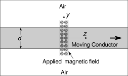
Figure 1: Schematic of the 2D problem.

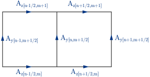
(a)

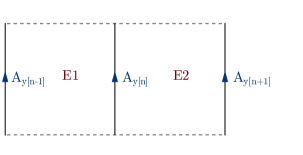
(b)

Figure 2: Representation of $\bf{A}$ with edge elements in $zy$-plane (a) 2D (b) reduced 1D.

For this 2D problem, the vector potential has components of $A_{y}$ and $A_{z}$. The same has been depicted in Fig.2a. In Fig.2a, the finite element discretisation of the 2D problem using edge elements is shown for one $y$-edge ([n,m+1/2]). For the sake of mathematical analysis, a simplified version with equal discretisation along the $z$ and $y$ axis is chosen. The edge variables are subscripted with $n$ and $m$, where $n$ denotes the progression along the $z$ axis and $m$ denotes the progression along the $y$ axis. It can be noted that, in addition to the integer progression ($n-1$, $n$, $n+1$), a factor of $1/2$ is present to denote the edge variable that is constant for the edge.

Now, let us consider the limiting case of $d\to\infty$ as described in [19]. Here, due to the symmetry along $y$-axis, the variations with respect to $y$-axis vanishes, resulting in a problem which is independent of $\phi$ and $A_{z}$. This situation is depicted in Fig.2b, wherein only $A_{y}$ has variations along the $z$-axis as is the case for $y$ directed edges which have the natural variation along the $z$-axis (perpendicular axis). The corresponding finite element formulation using the edge elements can be written as,

$$\begin{split}\int_{\Omega}\dfrac{d{M_{y}^{l}}}{dz}\frac{d{{A}_{y}}}{dz}~{}d\Omega+\mu\sigma u_{z}\int_{\Omega}M_{y}^{l}\frac{d{{A}_{y}}}{dz}~{}d\Omega~{}\dots{\\ }=\mu\sigma u_{z}\int_{\Omega}M_{y}^{l}{B}_{x}\end{split}$$ (3)

where, $M_{y}^{l}$ is the $y$-directed edge weight function [28]. Evaluating the above equation for the $n^{th}$ edge gives the following difference equation,

$$\begin{split}-(1+P_{e})A_{y[n-1]}+2A_{y[n]}-(1-P_{e})A_{y[n+1]}~{}\dots{\\ }=\frac{1}{3}(B_{x[n-1]}+4*B_{x[n]}+B_{x[n+1]})*P_{e}*\Delta z\end{split}$$ (4)

This is same as that of the nodal formulation as in [20]. The numerical instability due to the negative roots (poles) of the difference equation can also be viewed with the help of $z$-transform [19, 20]. Moreover, the $z$-transform clearly shows the effect of zeros arising from the source term as well. Applying the $Z$-transform on (4),

$$\frac{A_{y}}{B_{x}}=\frac{(Z+0.27)(Z+3.73)P_{e}\Delta z}{3(-1+P_{e})(Z-1)(Z-\dfrac{-1-P_{e}}{-1+P_{e}})}$$ (5)

For $P_{e}>>$ 1, the above equation (5) reduces to,

$$\frac{A_{y}}{B_{x}}\simeq\frac{\Delta z}{3}\frac{(Z+0.27)(Z+3.73)}{(Z-1)(Z+1)}$$ (6)

Now, the pole at -1 of equation (6) leads to the oscillation in the solution.

Here, the relation between $A_{y}$ and $B_{x}$ in (6) is found to be same as that of in [20] with the nodal formulation. The oscillation appearing in the solution in [20] is successfully mitigated by applying the input field $B_{x}$ as the averaged nodal flux densities for the element. Here, the same approach is extended for the edge formulation, with elemental input fields, $B_{xE1}$, $B_{xE2}$. The $B_{xE1}$ and $B_{xE2}$ are the element-averaged input magnetic fields for the elements spanning $[n-1],[n]$ and $[n],[n+1]$ respectively. The $B_{xE1}$ and $B_{xE2}$ are defined as [20],

$$B_{xE1}=(B_{x[n-1]}+B_{x[n]})/2$$

$$B_{xE2}=(B_{x[n]}+B_{x[n+1]})/2$$

For these modified inputs, the difference equation for (3) becomes,

$$\begin{split}-(1+P_{e})A_{y[n-1]}+2A_{y[n]}-(1-P_{e})A_{y[n+1]}~{}\dots{\\ }=\frac{1}{2}(B_{x[n-1]}+2*B_{x[n]}+B_{x[n+1]})*P_{e}*\Delta z\end{split}$$ (7)

Applying the $Z$-transform,

$$\frac{A_{y}}{B_{x}}=\frac{(Z+1)^{2}P_{e}\Delta z}{2(-1+P_{e})(Z-1)(Z-\dfrac{-1-P_{e}}{-1+P_{e}})}$$ (8)

For $P_{e}>>$ 1, the above equation (8) reduces to,

$$\frac{A_{y}}{B_{x}}\simeq\frac{\Delta z}{2}\frac{(Z+1)}{(Z-1)}$$ (9)

While comparing (9) with (6), one would readily recognize that for high Peclet number, the zero at -1 for the second case eventually cancels the oscillatory pole at -1, thus leading to a stable solution. This indicates that the elemental average of the input magnetic field can be used for the edge elements as well. However, further confirmation in 2D would be helpful, since the edge elements are generally designed for curl problems. The stability analysis in 2D is dealt in the next subsection.

II-B Analysis with the 2D version of the problem

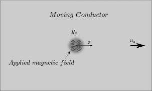
Figure 3: Schematic of the simplified 2D problem for the stability analysis

A simplified, 2D version of the moving conductor problem as shown in Fig. 3 is considered. The governing equations for the same are given below,

$$\nabla\cdot(\sigma\nabla\phi)-\nabla\cdot(\sigma{\bf u}\times(\nabla\times{\bf A}))=\nabla\cdot(\sigma u_{z}B_{x}{\bf\hat{y}})$$ (10)

$$\sigma\nabla\phi-\nabla\cdot\dfrac{1}{\mu}(\nabla{\bf A})-\sigma{\bf u}\times(\nabla\times{\bf A})=\sigma u_{z}B_{x}{\bf\hat{y}}$$ (11)

In the edge element formulation, the magnetic vector potential $\bf{A}$ is modeled with the edge vector shape functions $\bf{M}$ [28]. For this cartesian case, the $y$-component of the vector potential would be modeled with $y$-directed edge shape functions, and similarly, the $z$-component of the vector potential would be modeled with $z$-directed edge shape functions. The electric scalar potential $\phi$ is modeled with the nodal shape functions $N$. In the Galerkin finite element formulation, the weight functions are the shape functions themselves, and to mark the difference the weight functions are super-scripted with $l$.

The Galerkin finite element formulation for the equations (10), (11) can be written as,

$$\begin{split}\int_{\Omega}\dfrac{d{N^{l}}}{dz}\dfrac{d{\phi}}{dz}~{}d\Omega+\int_{\Omega}\dfrac{d{N^{l}}}{dy}\dfrac{d{\phi}}{dy}~{}d\Omega+u_{z}\int_{\Omega}\dfrac{d{N^{l}}}{dy}\dfrac{d{A_{y}}}{dz}~{}d\Omega~{}\dots{\\ }-u_{z}\int_{\Omega}\dfrac{d{N^{l}}}{dy}\dfrac{d{A_{z}}}{dy}~{}d\Omega=u_{z}\int_{\Omega}\dfrac{d{N^{l}}}{dy}{B}_{x}\end{split}$$ (12)

$$\begin{split}\mu\sigma\int_{\Omega}M_{y}^{l}\dfrac{d{\phi}}{dy}~{}d\Omega+\int_{\Omega}\dfrac{d{M_{y}^{l}}}{dz}\frac{d{{A}_{y}}}{dz}~{}d\Omega+\int_{\Omega}\dfrac{d{M_{y}^{l}}}{dy}\frac{d{{A}_{y}}}{dy}~{}d\Omega~{}\dots{\\ }+\mu\sigma u_{z}\int_{\Omega}M_{y}^{l}\frac{d{{A}_{y}}}{dz}~{}d\Omega-\mu\sigma u_{z}\int_{\Omega}M_{y}^{l}\frac{d{{A}_{z}}}{dy}~{}d\Omega~{}\dots{\\ }=\mu\sigma u_{z}\int_{\Omega}M_{y}^{l}{B}_{x}\end{split}$$ (13)

$$\mu\sigma\int_{\Omega}M_{z}^{l}\dfrac{d{\phi}}{dz}~{}d\Omega+\int_{\Omega}\dfrac{d{M_{z}^{l}}}{dz}\frac{d{{A}_{z}}}{dz}~{}d\Omega+\int_{\Omega}\dfrac{d{M_{z}^{l}}}{dy}\frac{d{{A}_{z}}}{dy}~{}d\Omega=0$$ (14)

It can be noted that, the equations (13), (14) are the weighted residual formulation of the equation (11); the former arise from the $y$-directed edge weight function ${\bf M}^{l}=M_{y}^{l}$ and the latter arise from the $z$-directed edge weight function ${\bf M}^{l}=M_{z}^{l}$. In addition to this, for the rest of the analysis, the element lengths along the $y$ and $z$-directions are assumed to be equal i.e. $\Delta y=\Delta z$ [20].

     

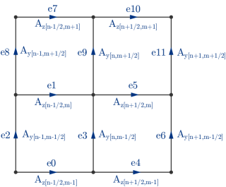
(a)

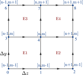
(b)

Figure 4: Representation of edge elements in 2D $zy$-plane (a) $z$ and $y$ directed edge vectors and their corresponding edge numbers (b) node and element numbering for the same set of edge elements.

The difference form of the finite element equation (12) for node-4 (see Fig. 4) can be written as,

$$\begin{split}\dfrac{1}{6}(2(\phi_{[0]}+\phi_{[1]}+\phi_{[2]}+\phi_{[3]}-8\phi_{[4]}+\phi_{[5]}+\phi_{[6]}~{}\dots{\\ }+\phi_{[7]}+\phi_{[8]})+3u_{z}(A_{[e2]}-A_{[e0]}-A_{[e4]}-A_{[e6]}~{}\dots{\\ }+A_{[e10]}-A_{[e8]}+A_{[e11]}-A_{[e7]}))~{}\dots{\\ }=\dfrac{u_{z}\Delta y}{12}(B_{x[8]}+B_{x[6]}+4B_{x[7]}-B_{x[0]}~{}\dots{\\ }-4B_{x[1]}-B_{x[2]})\end{split}$$ (15)

In the above equation, it may be noted that the scalar variable $\phi$ is at the nodes, whereas, the vector potential $A_{[e]}$ is present at the edges. The stability analysis requires the variables to be at the nodes [20, 29, 30]. Therefore, it is necessary to represent the vector potential at the nodes. For this, the node equivalent of the vector potential is obtained by averaging the vector potential at the edges. Each node has two $y$-directed edges (vertical edges); by taking the average of the two, the $A_{y[node]}$ is obtained. Similarly, each node has two $z$-directed edges (horizontal edges); by taking the average of the two, the $A_{z[node]}$ is obtained. With these, the nodal form of the (15) can be written as,

$$\begin{split}\dfrac{1}{6}(2(\phi_{[0]}+\phi_{[1]}+\phi_{[2]}+\phi_{[3]}-8\phi_{[4]}+\phi_{[5]}+\phi_{[6]}~{}\dots{\\ }+\phi_{[7]}+\phi_{[8]})+\dfrac{3u_{z}}{2}(A_{y[0]}+A_{y[8]}-A_{y[2]}-A_{y[6]})~{}\dots{\\ }+3u_{z}(-A_{z[1]}+A_{z[7]}))~{}\dots{\\ }=\dfrac{u_{z}\Delta y}{12}(B_{x[8]}+B_{x[6]}+4B_{x[7]}-B_{x[0]}~{}\dots{\\ }-4B_{x[1]}-B_{x[2]})\end{split}$$ (16)

For the vector equation, the 2D representation (see Fig. 4a) has two edges for each direction. That is, the shape function corresponds to edges $e3,~{}e9$, each form a finite element equation. Similarly, the shape function corresponds to edges $e1,~{}e5$, each form a finite element equation. Thus, there are 4 finite element equations associated with 4-edges. In contrast, the node element form only one equation that corresponds to node-4. The edges $e1,~{}e5$ are directed along the $z$ direction; so their Galerkin weighted residual formulation corresponds to the $z$ component of the vector equation (11). Then, the difference form of the finite element equation (14) for $e1$ can be written as,

$$\begin{split}-\dfrac{1}{6}((\phi_{[0]}-\phi_{[1]}+4\phi_{[3]}-4\phi_{[4]}+\phi_{[6]}-\phi_{[7]})\Delta y^{2}\mu\sigma~{}\dots{\\ }+6(A_{[e0]}-2A_{[e1]}+A_{[e7]})\Delta z)/(\Delta y^{2}\Delta z\mu)=0\end{split}$$ (17)

Similarly, the difference form of the finite element equation (14) for $e5$ can be written as,

$$\begin{split}-\dfrac{1}{6}((\phi_{[1]}-\phi_{[2]}+4\phi_{[4]}-4\phi_{[5]}+\phi_{[7]}-\phi_{[8]})\Delta y^{2}\mu\sigma~{}\dots{\\ }+6(A_{[e10]}-2A_{[e5]}+A_{[e4]})\Delta z)/(\Delta y^{2}\Delta z\mu)=0\end{split}$$ (18)

Upon taking the average of equations (17) and (18), one gets the averaged difference form of the finite element equation (14) along $z$-direction.

$$\begin{split}-\dfrac{1}{6}((\phi_{[0]}-\phi_{[2]}+4\phi_{[3]}-4\phi_{[5]}+\phi_{[6]}-\phi_{[8]})\Delta y^{2}\mu\sigma~{}\dots{\\ }+6(A_{[e0]}-2A_{[e1]}+A_{[e4]}-2A_{[e5]}+A_{[e7]}~{}\dots{\\ }+A_{[e10]})\Delta z)/(\Delta y^{2}\Delta z\mu)=0\end{split}$$ (19)

The above equation (19) is in terms of the edge vectors $A_{[e]}$. By following the similar procedure that applies for (16), the edge variables are represented with their respective node equivalents,

$$\begin{split}-\dfrac{1}{6}((\phi_{[0]}-\phi_{[2]}+4\phi_{[3]}-4\phi_{[5]}+\phi_{[6]}-\phi_{[8]})\Delta y^{2}\mu\sigma~{}\dots{\\ }+12(A_{z[1]}-2A_{z[4]}+A_{z[7]})\Delta z)/(\Delta y^{2}\Delta z\mu)=0\end{split}$$ (20)

By following the same procedure for the $y$ directed edges; that is i) obtain the difference equations of the Galerkin formulation from $e3$ and $e9$ edges ii) average them iii) represent the edge variables with their node equivalents. After these 3-steps, the final difference equation for (13) can be written as,

$$\begin{split}-\dfrac{1}{6}((\phi_{[0]}+4\phi_{[1]}+\phi_{[2]}-\phi_{[6]}-4\phi_{[7]}-\phi_{[8]})\Delta z\mu\sigma~{}\dots{\\ }-6(-A_{y[3]}+A_{y[5]}+A_{z[1]}-A_{z[7]})\mu\sigma u_{z}\Delta z~{}\dots{\\ }+12(A_{y[3]}-2A_{y[4]}+A_{y[5]}))/(\Delta z^{2}\mu)~{}\dots{\\ }=\dfrac{1}{12}(B_{x[0]}+4B_{x[1]}+B_{x[2]}+2B_{x[3]}+8B_{x[4]}~{}\dots{\\ }+2B_{x[5]}+B_{x[6]}+4B_{x[7]}+B_{x[8]})\sigma u_{z}\end{split}$$ (21)

The equations (16), (20), (21) forms a system of 3 equations and 3 variables $\phi,A_{y},A_{z}$. The stability analysis can be now performed by taking 2D $Z$-transform of these equations [29, 31, 20]. In this, the $z$-direction is represented by the transformation variable $Z_{n}$ and the $y$-direction is represented by the transformation variable $Z_{m}$ (please refer to Fig. 4b). After taking 2D $Z$- transform, the equations (16), (21), (20) take the following form,

$$\begin{split}\dfrac{1}{3}[S1]\phi+\dfrac{u_{z}}{4}[S2]A_{y}-\dfrac{u_{z}}{2}[S3]A_{z}=\dfrac{u_{z}\Delta z}{12}[Q1]B_{x}\end{split}$$ (22)

$$\begin{split}\dfrac{Pe}{6u_{z}}[Q1]\phi+(-[S1]+Pe[Q2])A_{y}+Pe[S3]A_{z}~{}\dots{\\ }=\dfrac{Pe\Delta z}{12}[M1]B_{x}\end{split}$$ (23)

$$\begin{split}\dfrac{Pe}{6u_{z}}[Q2^{\prime}]\phi-[S1^{\prime}]A_{z}=0\end{split}$$ (24)

where,

$$[Q1]=Z_{n}^{2}Z_{m}^{2}+4Z_{n}Z_{m}^{2}+Z_{m}^{2}-Z_{n}^{2}-4Z_{n}-1$$ (25)

$$[Q2]=Z_{n}^{2}Z_{m}-Z_{m}$$ (26)

$$[Q2^{\prime}]=Z_{n}^{2}Z_{m}^{2}-Z_{m}^{2}+4Z_{n}^{2}Z_{m}-4Z_{m}+Z_{n}^{2}-1$$ (27)

$$\begin{split}[S1]=1+Z_{n}+Z_{n}^{2}+Z_{m}+Z_{n}^{2}Z_{m}+Z_{m}^{2}~{}\dots{\\ }+Z_{n}Z_{m}^{2}+Z_{n}^{2}Z_{m}^{2}-8Z_{n}Z_{m}\end{split}$$ (28)

$$[S2]=1+Z_{n}^{2}Z_{m}^{2}-Z_{n}^{2}-Z_{m}^{2}$$ (29)

$$[S3]=Z_{n}-Z_{n}Z_{m}^{2}$$ (30)

$$[S1^{\prime}]=Z_{n}-2Z_{n}Z_{m}+Z_{n}Z_{m}^{2}$$ (31)

$$\begin{split}[M1]=1+4Z_{n}+Z_{n}^{2}+2Z_{m}+8Z_{n}Z_{m}~{}\dots{\\ }+2Z_{n}^{2}Z_{m}+Z_{m}^{2}+4Z_{n}Z_{m}^{2}+Z_{n}^{2}Z_{m}^{2}\end{split}$$ (32)

The equations (22), (23) and (24) form a system of 3 equations with 3 variables $\phi,A_{y},A_{z}$. By following a similar procedure as that of [20], the final equation is obtained for $Pe>>1$ as,

$$\begin{split}\left([Q2][S3])+\dfrac{[S3][S2]}{2}\right)A_{y}\approx\dfrac{\Delta z}{12}(~{}[M1][S3]~{}\dots{\\ }+2[Q1][S3]~{})B_{x}\end{split}$$ (33)

Upon simplification, the transfer function takes the following form,

$$\dfrac{A_{y}}{B_{x}}\approx\dfrac{\Delta z}{6}\dfrac{(Z_{n}^{2}+4Z_{n}+1)f1(Z_{m})}{(1-Z_{n}^{2})f2(Z_{m})}$$ (34)

where,

$$f1(Z_{m})=1-2Z_{m}-3Z_{m}^{2}$$

$$f2(Z_{m})=(2Z_{m}-(1-Z_{m}^{2})^{2})$$

The transfer function (34) has poles/roots located at $-1,+1$, among which the pole at ‘-1’ causes the oscillatory behaviour in the solution. The zeros are located at $Z_{n}=-0.27,-3.7$. The locations of the zeros may be changed by modifying the representation of the input magnetic field consistently. By following the 1D case (please refer to II-A) and the preceding work [20], the input magnetic field, which is directed along $x$-edges (perpendicular to the plane) can be averaged over each element and the resultant magnetic field can be used as the input field. In other words, the following would be the input field for the element $E1$,

$$\begin{split}B_{x}=\dfrac{1}{4}(B_{x}[n-1,m-1]+B_{x}[n,m-1]\dots{\\ }+B_{x}[n-1,m]+B_{x}[n,m])\end{split}$$ (35)

and similarly for other elements. With this modification, the transfer function for the proposed formulation is calculated to take the following form,

$$\dfrac{A_{y}}{B_{x}} \approx\dfrac{\Delta z}{4}\dfrac{(Z_{n}^{2}+2Z_{n}+1)f1(Z_{m})}{(1-Z_{n}^{2})f2(Z_{m})}$$

$$\approx\dfrac{\Delta z}{4}\dfrac{(1+Z_{n})\bcancel{(1+Z_{n})}f1(Z_{m})}{(1-Z_{n})\bcancel{(1+Zn)}f2(Z_{m})}$$ (36)

The oscillatory pole at ‘$Z=-1$’ is canceled by the zero introduced in the numerator. Thus, the elemental averaging of the input magnetic field can be seen to possess the stability properties similar to that of 1D. In the next section, numerical validation exercises are carried out in 2D and 3D.

III Numerical Validation

III-A Simulation Results for 2D version of the problem

Figure 5: Sample 2D finite element mesh

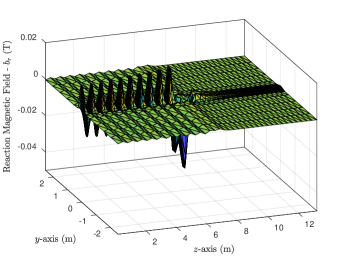
(a)

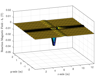
(b)

Figure 6: Reaction magnetic field - $b_{x}$ from the 2D moving conductor problem with $Pe=200$ (a) Galerkin formulation (b) Proposed formulation

The 2D simulation involves the problem setup, shown in Fig. 1. The corresponding finite element mesh is shown in Fig. 5. The physical parameters of the problem are as follows. The conductor has a width of $d=0.5m$, its conductivity is $\sigma=7.2\times 10^{6}Sm^{-1}$ and its velocity is $u_{z}=50ms^{-1}$. Simulations were carried out to test the stability of the proposed formulation; stable solutions are observed. A sample simulation result showing the reaction magnetic field $b_{x}=\partial A_{z}/\partial y-\partial A_{y}/\partial z$ with $Pe=200$ is displayed in Fig. 6. The Fig. 6a shows the $b_{x}$ obtained from the standard Galerkin formulation and the Fig. 6b shows the same from the proposed formulation. It can be seen that the proposed formulation gives a stable solution without any numerical oscillations.

In the nodal formulation, it was possible to obtain the analytical expression for the peak errors due to the numerical oscillation [20]. This is because, the nodal formulation can be reduced to 1D and the resulting finite element equation in the difference form can be solved. The following expressions of peak errors are derived in [20].

Analytical error in the standard Galerkin formulation:

$$\hat{e}_{GA}=\left|\dfrac{(Pe^{2}-3)(Pe-1)}{3(Pe+1)^{3}}\right|\times 100\%$$ (37)

Analytical error in the stable nodal formulation of [20]:

$$\hat{e}_{SA}=\left|\dfrac{Pe-1}{(Pe+1)^{3}}\right|\times 100\%$$ (38)

Figure 7: % Peak error measured

Having these nodal errors as reference, the peak oscillation error with the edge elements are measured for the 2D problem. These measured values are plotted in Fig. 7, where $\hat{e}_{GN}$ is the peak error measured with the Galerkin formulation and $\hat{e}_{SN}$ is the peak error measured with the Proposed formulation. It is observed that the peak error from the 2D-Galerkin-Edge is twice that of the 1D-Galerkin-Node. In other words, ‘$\hat{e}_{GN}\approx 2~{}\hat{e}_{GA}$’ and the same can observed from the plot of ‘$2~{}\hat{e}_{GA}$’ in Fig. 7. It can also be observed that the peak error measured with the proposed formulation ($\hat{e}_{SN}$) is negligible.

TABLE I: Measured values of Error in the first derivative for Galerkin scheme and the proposed scheme

		Error measured in $b_{x}=\nabla\times{\bf A}\cdot\hat{x}$, normalised w.r.t. applied magnetic field $B_{ax}$
Number of Elements	$P_{e}$	Galerkin Formulation			Proposed Formulation
		L2 Error	Absolute Error	Expt. Order of Convergence	L2 Error	Absolute Error	Expt. Order of Convergence
640	100	6.035e-04	1.213e-01	-	1.765e-04	1.594e-02	-
2560	50	4.634e-04	8.741e-02	0.47	1.210e-04	8.650e-03	0.88
10240	25	2.708e-04	4.327e-02	1.01	7.919e-05	3.988e-03	1.12
40960	12.5	1.218e-04	1.220e-02	1.83	4.558e-05	1.509e-03	1.40

In table I, the average and the rms error measured for the first derivative (reaction magnetic field $b_{x}$) is presented. The errors measured for the Galerkin scheme and the proposed scheme, for different amount of resolution. The average error, as well as, the rms (L2) error are observed to fall with the increasing resolution. It may also be noted that the errors measured from the proposed scheme are an order of magnitude smaller than the errors measured from the Galerkin scheme. With the increasing resolution, the proposed formulation also produces the expected convergence rate. Thus, the proposed formulation gives stable, as well as, accurate results. In the next subsection, further testing is carried out in 3D with the ‘Testing Electromagnetic Analysis Methods’ (TEAM) problem No. 9 [32].

III-B Validation with 3D TEAM-9 problem

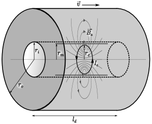
(a)

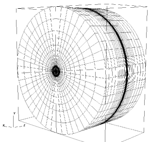
(b)

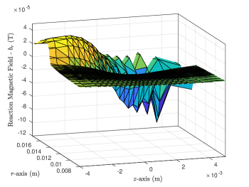
(c)

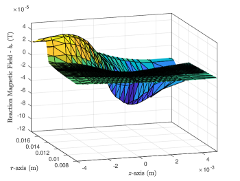
(d)

Figure 8: Description of the TEAM 9a problem and sample results (a) Schematic representation of the TEAM 9a moving conductor problem. (b) Finite element mesh employed (c) Galerkin scheme - reaction magnetic field - $b_{r}$ for $u_{z}$ = 100 $ms^{-1}$ and $\mu_{r}$ = 50 (d) Proposed scheme - reaction magnetic field - $b_{r}$ for $u_{z}$ = 100 $ms^{-1}$ and $\mu_{r}$ = 50 in the cross section along $rz$ plane for $\theta\approx 0^{o}$.

A schematic diagram of the TEAM-9 problem is shown in Fig. 8a. The problem has an infinite ferromagnetic material with the conductivity of $\sigma=5\times 10^{6}~{}Sm^{-1}$. The relative magnetic permeability of the material is taken as $\mu_{r}=1$ and $\mu_{r}=50$. The ferromagnetic material has a cylindrical bore with the radius of $r_{i}=14\times 10^{-3}m$. A concentric current-carrying loop with $1A$ of current and a radius of $r_{c}=12\times 10^{-3}m$ is moving at an uniform velocity inside the bore. For the analysis, the case with the largest velocity ($v=100ms^{-1}$) is chosen. In order to accurately model the current loop, the finite element mesh close to the current loop is dense; away from the current loop, the mesh becomes progressively coarser. Due to this variation, the resulting value of the Peclet number varies from $5$ to $200$. The finite element mesh employed is shown in Fig. 8b. In the proposed formulation, for each element, the $x,y,z$ components of the applied magnetic field $B_{x},B_{y},B_{z}$ are represented as,

$$B_{x}=\dfrac{1}{\sum_{e=1}^{n}|v^{e}_{x}|}\sum_{e=1}^{n}B^{e}v^{e}_{x}$$ (39)

$$B_{y}=\dfrac{1}{\sum_{e=1}^{n}|v^{e}_{y}|}\sum_{e=1}^{n}B^{e}v^{e}_{y}$$ (40)

$$B_{z}=\dfrac{1}{\sum_{e=1}^{n}|v^{e}_{z}|}\sum_{e=1}^{n}B^{e}v^{e}_{z}$$ (41)

where $n$ is the number of edges for each element, $B^{e}$ is the applied magnetic field corresponding to each edge, and $v_{x}^{e},v_{y}^{e},v_{z}^{e}$ form the unit vector ${\bf v}_{e}=\{v_{x}^{e},v_{y}^{e},v_{z}^{e}\}$ of the edge ‘$e$’. The elemental applied magentic field vector ${\bf B}=\{B_{x},B_{y},B_{z}\}$ is the source field in the proposed formulation. The standard Galerkin formulation would have the applied magnetic field at each Gauss-integration point ${\bf B}_{g}$ as,

$${\bf B}_{g}=\sum_{e=1}^{n}B^{e}{\bf M}_{g}^{e}$$

where ${\bf M}^{e}_{g}$ is the value of edge shape function vector at a Gauss-integration point. The simulated, reaction magnetic field along the $rz$-plane is plotted in Fig. 8c and Fig. 8d for the Galerkin scheme and the proposed formulation, respectively. It may be readily noted that the $b_{r}$ from the proposed formulation is stable as expected.

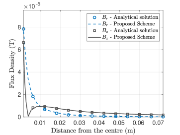
(a)

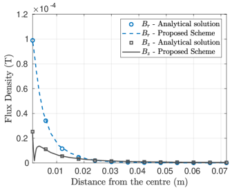
(b)

Figure 9: Comparison of the total magnetic flux densities from the analytical solution of the TEAM-9 problem [32] and the proposed formulation; for the cases of (a) $u_{z}=100ms^{-1}$, $\mu_{r}=1$ (b) $u_{z}=100ms^{-1}$, $\mu_{r}=50$

The TEAM-9 test problem is also provided with the set of analytical solution for comparison [32]. It may be noted that, the analytical solutions are provided along the radius of $r=13mm$, which is $1mm$ away from both the current carrying coil and the ferromagnetic cylinder. Since the measurement point is very close to the cylinder, as well as, the circular coil, it is necessary to model them as accurately as possible. Such a modeling is not feasible with linear edge elements in cartesian coordinate system. Therefore, the problem is transferred to the cylindrical coordinate system for the accuracy study. In the cylindrical coordinate system, the results of Fig. 8c and Fig. 8d are once again observed. In addition to this, edge elements can accurately represent the simulation domain in cylindrical coordinate system. Simulations are carried out for $v=100ms^{-1}$ with $\mu_{r}=1$, as well as, the ferromagnetic case of $\mu_{r}=50$. The results from $r=13mm$ are plotted along with the analytical solution in Fig. 9. It can be seen that the proposed formulation performs consistently in 3D as well.

IV Discussion on Mesh

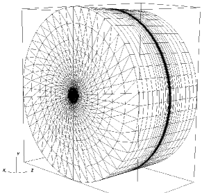
(a)

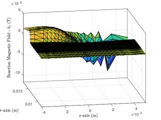
(b)

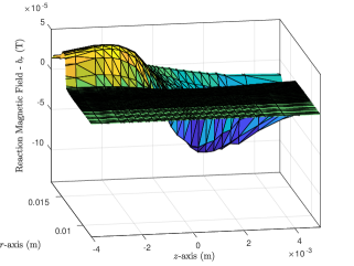
(c)

Figure 10: Sample results from TEAM 9a problem with wedge elements (a) Finite element mesh with wedge elements (b) Galerkin scheme - reaction magnetic field - $b_{r}$ for $u_{z}$ = 100 $ms^{-1}$ and $\mu_{r}$ = 50 (c) Proposed scheme - reaction magnetic field - $b_{r}$ for $u_{z}$ = 100 $ms^{-1}$ and $\mu_{r}$ = 50 in the cross section along $rz$ plane for $\theta\approx 0^{o}$.

The present work deals with the simulation of linear moving conductor problems such as, electromagnetic brakes, linear induction motor, electromagnetic flowmeter etc. In such cases, the conducting region of the problem can be and usually be discretised with graded regular mesh along the moving direction. In other words, the resulting mesh would look like a stack of layers of different thickness along the moving direction. The same can be seen in Fig. 8b. In this, the discretisation along the direction of motion ($z$-axis) has dense discretisation close to the center, where the current loop is present and the discretisation becomes coarser as we move away from the center.

The source based stabilisation strategies utilize this feature of the linear moving conductor problems. Here, the stabilisation is brought in by the pole-zero cancellation of the source term. Such an analysis is valid, only when the discretisation is like a stack of layers along the moving direction. Hence, the proposed scheme requires a regular mesh in 2D with quadrilateral elements. In the case of 3D, the restriction only applies to the direction of motion. Therefore, the cross section of the moving conductor, i.e., the plane perpendicular to the motion, can be discretised without any restrictions. Hence, the 3D problems can be discretised with hexahedral or wedge elements. The discretisation using hexahedral elements is shown in Fig. 8b.

The application of wedge elements with vector shape functions are scarce in literature. However, the vector shape functions for the wedge elements are straight forward to derive and they are provided in Appendix A for quick reference. The discretisation using wedge elements for the TEAM-9 test problem is shown in Fig. 10a. The simulated reaction magnetic field, along the $rz$-plane is plotted in Fig. 10b and Fig. 10c for the Galerkin scheme and the proposed formulation, respectively. The $b_{r}$ from the proposed formulation is stable as expected, with the wedge elements as well. As an added note, the discussion in this section is also applicable to node elements [20].

V Summary and Conclusion

Edge elements are vital in the finite element simulation of electromagnetic fields, especially when multiple materials are present and the simulation variables are electric and magnetic fields themselves. Like many other central-weighted numerical schemes, edge elements also produce numerically oscillating solutions for the simulation of moving conductor problems at high velocities. In such a situation, the usual strategy is to employ the upwinding strategies, which in a way introduce extra diffusion to stabilize the solution [18, 22, 23]. However, the upwinding schemes are known to be susceptible to transverse-boundary error at the material interfaces [25, 27, 21, 24].

In this work, the source-based stabilization strategies which are proposed for the nodal formulation, are extended for the edge elements. The formulation require a graded regular mesh along the direction of motion. The stability of the proposed formulation is analytically studied in 1D, as well as, 2D with edge elements. Then numerical exercises are carried out for the verification of the proposed formulation. The simulation results in 2D demonstrate that the formulation produces stable, accurate and converging solutions. The 3D simulation is carried out with the TEAM-9 problem and stable solutions are observed. Comparing the analytical solutions of the TEAM-9 problem and the simulation results, accuracy of the proposed formulation is demonstrated in 3D.

Appendix A Wedge element - vector shape functions

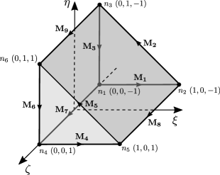
Figure 11: Wedge element in $(\xi,\eta,\zeta)$ coordinate system. $n$-denotes the nodes of the element. $\mathbf{M}$-denotes the vector shape functions, corresponds to each edge.

The edge shape functions for the wedge element are provided below. Consider the reference triangle element in $(\xi,\eta)$ coordinate system with its nodes $a,b,c$ located at $(0,0)$, $(1,0)$, $(0,1)$ respectively. The node shape functions for this reference triangle element can be written as [33],

$$N_{a} =1-\xi-\eta$$

$$N_{b} =\xi$$

$$N_{c} =\eta$$ (42)

Using these, the vector shape function of the wedge element can be constructed. The reference wedge element in $(\xi,\eta,\zeta)$ coordinate system is shown in Fig. 11. The edge shape functions for the wedge element are:

$${\bf M_{1}} =l_{1}(N_{a}~{}\nabla N_{b}-N_{b}~{}\nabla N_{a})\dfrac{(1-\zeta)}{2}$$

$${\bf M_{2}} =l_{2}(N_{b}~{}\nabla N_{c}-N_{c}~{}\nabla N_{b})\dfrac{(1-\zeta)}{2}$$

$${\bf M_{3}} =l_{3}(N_{c}~{}\nabla N_{a}-N_{a}~{}\nabla N_{c})\dfrac{(1-\zeta)}{2}$$

$${\bf M_{4}} =l_{4}(N_{a}~{}\nabla N_{b}-N_{b}~{}\nabla N_{a})\dfrac{(1+\zeta)}{2}$$

$${\bf M_{5}} =l_{5}(N_{b}~{}\nabla N_{c}-N_{c}~{}\nabla N_{b})\dfrac{(1+\zeta)}{2}$$

$${\bf M_{6}} =l_{6}(N_{c}~{}\nabla N_{a}-N_{a}~{}\nabla N_{c})\dfrac{(1+\zeta)}{2}$$

$${\bf M_{7}} =l_{7}N_{a}~{}\nabla\zeta/2$$

$${\bf M_{8}} =l_{8}N_{b}~{}\nabla\zeta/2$$

$${\bf M_{9}} =l_{9}N_{c}~{}\nabla\zeta/2$$ (43)

where, $l_{1},~{}l_{2},~{}\dots,~{}l_{9}$ are the actual lengths of the edges that correspond to edge shape function $\mathbf{M}$. The gradients are taken with respect to the ($x,y,z$) coordinate system [28].

Sujata Bhowmick (Member, IEEE) received the B.E. degree in electrical engineering from IIEST, Shibpur, India, in 2006, and the M.E. degree in electrical engineering from the Indian Institute of Science, Bengaluru, India, in 2011. She received the Ph.D. degree from the Department of Electronic Systems Engineering, Indian Institute of Science, Bengaluru, India, in 2019. Her current research interests include power electronics for renewable resources, single-phase grid-connected power converters, computational electromagnetics, finite element and edge element methods.

Sethupathy Subramanian received the bachelors degree in electrical and electronics engineering from Anna University, Chennai, India, in 2009. He received the masters and doctrate degrees in electrical engineering from Indian Institute of Science, Bangalore, India in 2011 and 2017 respectively. He also received masters and doctrate degrees in Physics from University of Notre Dame, USA in 2022 and 2023 respectively. His research interests, pertinent to electrical engineering, include computational electromagnetics, numerical stability, finite element and edge element methods.

References

- [1] O. Biro, K. Preis, W. Renhart, K. Richter, and G. Vrisk, “Performance of different vector potential formulations in solving multiply connected 3-d eddy current problems,” Magnetics, IEEE Transactions on, vol. 26, no. 2, pp. 438–441, 1990.
- [2] T. Shimizu, N. Takeshima, and N. Jimbo, “A numerical study on faraday-type electromagnetic flowmeter in liquid metal system, (i),” Journal of Nuclear Science and Technology, vol. 37, no. 12, pp. 1038–1048, 2000.
- [3] O. Zienkiewicz, R. Taylor, and P. Nithiarasu, The Finite Element Method for Fluid Dynamics. Elsevier Science, 2005.
- [4] D. Spalding, “A novel finite difference formulation for differential expressions involving both first and second derivatives,” International Journal for Numerical Methods in Engineering, vol. 4, no. 4, pp. 551–559, 1972.
- [5] I. Christie, D. F. Griffiths, A. R. Mitchell, and O. C. Zienkiewicz, “Finite element methods for second order differential equations with significant first derivatives,” International Journal for Numerical Methods in Engineering, vol. 10, no. 6, pp. 1389–1396, 1976.
- [6] M. Odamura, “Upwind finite element solution for saturated traveling magnetic field problems,” Electrical Engineering in Japan, vol. 105, no. 4, pp. 126–132, 1985.
- [7] M. Ito, T. Takahashi, and M. Odamura, “Up-wind finite element solution of travelling magnetic field problems,” Magnetics, IEEE Transactions on, vol. 28, no. 2, pp. 1605–1610, 1992.
- [8] D. Rodger, P. Leonard, and T. Karaguler, “An optimal formulation for 3d moving conductor eddy current problems with smooth rotors,” Magnetics, IEEE Transactions on, vol. 26, no. 5, pp. 2359–2363, 1990.
- [9] E. Chan and S. Williamson, “Factors influencing the need for upwinding in two-dimensional field calculation,” Magnetics, IEEE Transactions on, vol. 28, no. 2, pp. 1611–1614, 1992.
- [10] N. Allen, D. Rodger, P. Coles, S. Strret, and P. Leonard, “Towards increased speed computations in 3d moving eddy current finite element modelling,” Magnetics, IEEE Transactions on, vol. 31, no. 6, pp. 3524–3526, 1995.
- [11] D. Rodger, T. Karguler, and P. Leonard, “A formulation for 3d moving conductor eddy current problems,” Magnetics, IEEE Transactions on, vol. 25, no. 5, pp. 4147–4149, 1989.
- [12] J. Bird, T. Lipo et al., “A 3-d magnetic charge finite-element model of an electrodynamic wheel,” Magnetics, IEEE Transactions on, vol. 44, no. 2, pp. 253–265, 2008.
- [13] H. Vande Sande, H. De Gersem, and K. Hameyer, “Finite element stabilization techniques for convection-diffusion problems,” 7th International journal of theoretical electrotechnics, pp. 56–59, 1999.
- [14] L. Codecasa and P. Alotto, “2-d stabilized fit formulation for eddy-current problems in moving conductors,” Magnetics, IEEE Transactions on, vol. 51, no. 3, pp. 1–4, 2015.
- [15] Y. Liang, “Steady-state thermal analysis of power cable systems in ducts using streamline-upwind/petrov-galerkin finite element method,” Dielectrics and Electrical Insulation, IEEE Transactions on, vol. 19, no. 1, pp. 283–290, 2012.
- [16] S. Noguchi and S. Kim, “Magnetic field and fluid flow computation of plural kinds of magnetic particles for magnetic separation,” Magnetics, IEEE Transactions on, vol. 48, no. 2, pp. 523–526, 2012.
- [17] T.-P. Fries and H. G. Matthies, “A review of petrov–galerkin stabilization approaches and an extension to meshfree methods,” Technische Universitat Braunschweig, Brunswick, 2004.
- [18] E. Oñate and M. Manzan, “Stabilization techniques for finite element analysis of convection-diffusion problems,” Developments in Heat Transfer, vol. 7, pp. 71–118, 2000.
- [19] S. Subramanian and U. Kumar, “Augmenting numerical stability of the galerkin finite element formulation for electromagnetic flowmeter analysis,” IET Science, Measurement & Technology, vol. 10, no. 4, pp. 288–295, 2016.
- [20] ——, “Stable galerkin finite-element scheme for the simulation of problems involving conductors moving rectilinearly in magnetic fields,” IET Science, Measurement & Technology, vol. 10, no. 8, pp. 952–962, 2016.
- [21] S. Subramanian, U. Kumar, and S. Bhowmick, “On overcoming the transverse boundary error of the su/pg scheme for moving conductor problems,” IEEE Transactions on Magnetics, vol. 58, no. 1, pp. 1–8, 2021.
- [22] E. X. Xu, J. Simkin, and S. C. Taylor, “Streamline upwinding in a 3-d edge-element method modeling eddy currents in moving conductors,” IEEE transactions on magnetics, vol. 42, no. 4, pp. 667–670, 2006.
- [23] F. Henrotte, H. Heumann, E. Lange, and K. Hameyer, “Upwind 3-d vector potential formulation for electromagnetic braking simulations,” IEEE Transactions on Magnetics, vol. 46, no. 8, pp. 2835–2838, 2010.
- [24] S. Subramanian and S. Bhowmick, “A stable weighted residual finite element formulation for the simulation of linear moving conductor problems,” IEEE Journal on Multiscale and Multiphysics Computational Techniques, vol. 7, pp. 220–227, 2022.
- [25] V. John and P. Knobloch, “On spurious oscillations at layers diminishing (sold) methods for convection–diffusion equations: Part i–a review,” Computer Methods in Applied Mechanics and Engineering, vol. 196, no. 17, pp. 2197–2215, 2007.
- [26] ——, “On spurious oscillations at layers diminishing (sold) methods for convection–diffusion equations: Part ii–analysis for p1 and q1 finite elements,” Computer Methods in Applied Mechanics and Engineering, vol. 197, no. 21, pp. 1997–2014, 2008.
- [27] S. Subramanian and U. Kumar, “Existence of boundary error transverse to the velocity in su/pg solution of moving conductor problem,” in Numerical Electromagnetic and Multiphysics Modeling and Optimization (NEMO), 2016 IEEE MTT-S International Conference on. IEEE, 2016, pp. 1–2.
- [28] J.-M. Jin, The finite element method in electromagnetics. John Wiley & Sons, 2002.
- [29] A. D. Poularikas, Handbook of formulas and tables for signal processing. CRC Press, 1998, vol. 13.
- [30] D. Dudgeon, R. Mersereau, and R. Merser, Multidimensional digital signal processing. PH, 1995.
- [31] K. Ogata, Discrete-Time Control Systems, ser. Prentice-Hall International Editions. Prentice-Hall, 1987.
- [32] N. Ida, “Team problem 9 velocity effects and low level fields in axisymmetric geometries,” Proc. Vancouver TEAM Workshop, Jul. 1988.
- [33] J. Reddy, An Introduction to the Finite Element Method. McGraw-Hill Education, 2005.