FedAUXfdp: Differentially Private One-Shot Federated Distillation

Abstract

Federated learning suffers in the case of “non-iid” local datasets, i.e., when the distributions of the clients’ data are heterogeneous. One promising approach to this challenge is the recently proposed method FedAUX, an augmentation of federated distillation with robust results on even highly heterogeneous client data. FedAUX is a partially $(\epsilon,\delta)$-differentially private method, insofar as the clients’ private data is protected in only part of the training it takes part in. This work contributes a fully differentially private modification, termed FedAUXfdp. We further contribute an upper bound on the $l_{2}$-sensitivity of regularized multinomial logistic regression. In experiments with deep networks on large-scale image datasets, FedAUXfdp with strong differential privacy guarantees performs significantly better than other equally privatized SOTA baselines on non-iid client data in just a single communication round. Full privatization of the modified method results in a negligible reduction in accuracy at all levels of data heterogeneity.

1 Introduction

Federated learning (FL) is a form of decentralized machine learning, in which a global model is formed by an orchestration server aggregating the outcome of training on a number of local client models without any sharing of their private training data McMahan et al. (2017). Interest in federated learning has increased recently for its privacy and communication-efficiency advantages over centralized learning on mobile and edge devices Li et al. (2019); Sattler et al. (2021c). A classical mechanism for model aggregation in FL is federated averaging (FedAVG), where the locally trained models are weighted proportionally to the size of the local dataset. In each communication round of federated averaging, weight updates of the clients’ local models are sent to the orchestration server, averaged by the server, and the average is sent back to the federation of clients to initialize the next round of training McMahan et al. (2017).

Federated ensemble distillation (FedD), an often even more communication-efficient and accurate alternative to FedAVG, uses knowledge distillation to transfer knowledge from clients to server Itahara et al. (2020); Lin et al. (2020); Chen and Chao (2020); Sattler et al. (2021b). In FedD, clients and server share a public dataset auxiliary to the clients’ private data. The clients communicate the output of their privately trained models on the public distillation dataset to the server, which uses the average of these outputs as supervision for the distillation data in training the global model. In comparison to federated averaging, federated ensemble distillation offers additional privacy, as direct white box attacks are not possible for example, and allows combining different model architectures, making it appealing in an Internet-of-Things ecosystem Li et al. (2020); Chang et al. (2019); Li et al. (2021).

FedAUX is an augmentation of federated distillation, which derives its success from taking full advantage of the AUXiliary data. FedAUX uses this auxiliary data for model pretraining and relevance weighting. To perform the weighting, the clients’ output on each data point of the distillation dataset is individually weighted by a measure of similarity between that distillation datapoint and the client’s local data, called a ‘certainty score’. Weighting the outputs by the scores prioritizes votes from clients whose local data is more similar to the auxiliary/distillation data.

A major challenge of federated learning is performance when the distributions of the clients’ data are heterogeneous, i.e. performance on “non-iid” data, as is often the circumstance in real-world applications of FL Kairouz et al. (2021). FedAUX overcomes that challenge, performing remarkably more efficiently on non-iid data than other state-of-the-art federated learning methods, federated averaging, federated proximal learning, Bayesian federated learning, and federated ensemble distillation. For example on MobilenetV2, FedAUX achieves 64.8% server accuracy, while even the second-best method only achieves 46.7% Sattler et al. (2021a).

Despite its privacy benefits, federated distillation still presents a privacy risk to clients participating Papernot et al. (2017). Data-level differential privacy protects the clients’ data by limiting the impact of any individual datapoint on the model and quantifies the privacy loss associated to participating in training with parameters $(\epsilon,\delta)$. Both governments and private institutions are increasingly interested in securing their data using differential privacy.

Each client in the FedAUX method trains two models on their local dataset. Sattler et al. (2021a) privatize only the scoring model, leaving the classification model exposed. The clients’ data is accordingly only protected with differential privacy in part of the training it participates in. In this work, we add a local, data-level $(\epsilon,\delta)$-differentially private mechanism for this second model and appropriately modify the FedAUX method to apply said mechanism. We thereby contribute a ‘fully’ privatized version of FedAUX. Full differential privacy here is used as a way of describing our contribution of privacy over the original FedAUX method. We additionally give an upper bound on the $l_{2}$-sensitivity of regularized multinomial logistic regression. See Section 4.2 for background on differential privacy.

In results with deep neural networks on large scale image datasets at an ($\epsilon=0.6,\delta=2*10^{-5}$) level of differential privacy we compare fully differentially private FedAUXfdp with two privatized baselines, federated ensemble distillation and federated averaging in a single communication round. FedAUXfdp outperforms these baselines dramatically on the heterogeneous client data. Our method modifications achieve better results than FedAUX in a single communication round and we see a negligible reduction in accuracy of applying this strong amount of differential privacy to the modified FedAUX method.

In Section 3 we outline the original FedAUX, in Section 4 we explain our modification, including our privacy mechanism as well as background on differential privacy, and in Section 5 we detail the experimental set-up and highlight important results.

2 Related Work

Our method modifies Sattler et al. (2021a), who contributed a semi-differentially private FedAUX method. For a discussion of works related to the non-privacy aspects of FedAUX, we refer to their paper.

Cynthia Dwork introduced differential privacy Dwork and Roth (2014) and Kasiviswanathan et al. (2008) local differential privacy. Differential privacy bounds were greatly improved with the introduction of the moments accountant in Abadi et al. (2016).

In addition to quantifying privacy loss, differential privacy protects provably against membership inference attacks Shokri et al. (2017); Choquette-Choo et al. (2021), in which an adversary can determine if a data point participated in the training of a model. This can pose a privacy threat, for example, if participation in model training could imply a client has a particular disease or other risk factor. Alternatives for privatization in general include secure multi-party computation or homomorphic encryption, though neither protect against membership inference attacks Shokri et al. (2017). Others have combined local differential privacy and federated learning, notably Geyer et al. (2018); McMahan et al. (2018). While Sun and Lyu (2021) combined federated model distillation with differential privacy, they only attain robust results on non-iid data when the client and distillation data contains the same classes.

Our one-shot federated distillation approach uses model distillation to transfer the learning outcome in form of softlabels for a public distillation dataset. Zhou et al. (2021) use dataset distillation Wang et al. (2018) to design a communication-efficient and privacy-preserving one-shot FL mechanism.

3 FedAUX

3.1 Method

In FedAUX, there are two actors, the clients and the orchestration server. Each client, $i=1,\ldots,n$, has its own private, local, labeled dataset $D_{i}$. Auxiliary to the client data, is a public, unlabeled dataset $D_{aux}$. The auxiliary data is further split into the negative data $D^{-}$, used in training the certainty score models, and the distillation data $D_{distill}$, used for knowledge distillation.

There are three types of models, the clients’ scoring models, the clients’ classification models, and the server’s global model, which can all be decomposed into a feature extractor $h$ and linear or logistic regression classification head. Whether the full model or just the classification head is trained varies by model and we outline this next. In FedAUX four kinds of training are conducted (see Figure 1):

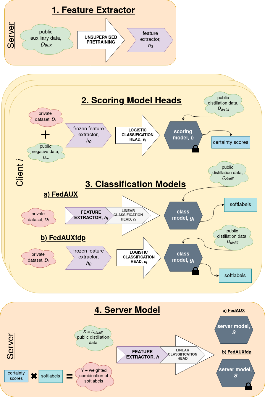
Figure 1: Overview of FedAUX and FedAUXfdp training. Models secured with differential privacy indicated with black locks.

1. Feature extractor. Unsupervised pretraining with the public auxiliary data $D_{aux}$ on the server to obtain the feature extractor, $h_{0}$, which is sent to the clients and initialized in all their models as well as the server’s.

2. Scoring model heads. Supervised training of the scoring model classification heads $s_{i}$ of all clients, in combination with the frozen feature extractor $h_{0}$ to generate scoring models $f_{i}=s_{i}\circ h_{0}$. Each training is a binary logistic regression on the extracted features of their private local data and the public negative data $h_{0}(D_{i}\cup D^{-})$.

3. Classification models. Supervised training of the clients’ full classification models $g_{i}=c_{i}\circ h_{i}$, consisting of a feature extractor $h_{i}$ (initialized with $h_{0}$ from the pretraining) and linear classification head $c_{i}$, on their local datasets $D_{i}$.

4. Server model. Supervised training of the server’s full model $S$, consisting of a feature extractor $h$ (initialized with $h_{0}$ from the pretraining) and linear classification head. The server calculates an initial weight update of the clients’ average class model weight updates from their training round. For the server’s training, the input data $X$ is the unlabeled $D_{distill}$ and the supervision $Y$ a $(|D_{distill}|\times n_{classes})$-dimensional matrix of the softlabel output of the class model $g_{i}(D_{distill})$, weighted by a certainty score for each distillation datapoint. The certainty scores are the output of the $(\epsilon,\delta)$-differentially privatized scoring model on the distillation data $f_{i}(D_{distill})$, measures of similarity between each distillation data point and the client’s local data. Each entry in $Y$ is:

   $$\frac{\sum_{i}f_{i}(x)\cdot g_{i}(x)}{\sum_{i}f_{i}(x)},\text{for }x\in D_{distill}.$$ (1)

3.2 Privacy

Participating in the training of the scoring classification heads and classification models presents a privacy risk to the private data of the clients. In FedAUX, the scoring heads are sanitized using an $(\epsilon,\delta)$-differentially private sanitization mechanism. FedAUX’s mechanism for privatizing the scoring model is based on freezing the feature extractor and using a logistic classification head. As the feature extractor was trained on public data, only sanitizing this head is required to yield a differentially private model. Further, using the L-BFGS optimizer in sci-kit learn’s logistic regression guarantees finding optimal weights for the logistic regression heads. In FedAUXfdp we privatize the classification models in a similar fashion. This thereby makes the server models learned in FedAUXfdp fully differentially private, as discussed in Section 4, with the specific privacy mechanism outlined in Section 4.2.

4 FedAUXfdp

In the fully differentially private version of FedAUX, we adapt the training of the classification and server models as follows. Rather than training the full client models, we freeze the feature extractors and train only the classification heads using a multinomial logistic regression on extracted features of the client’s local dataset $D_{i}$. As communicating model updates to the server poses a privacy threat, we no longer initialize the server with the averaged weight update of the clients. Accordingly, step three in the process is changed as follows:

1. Classification model. Supervised training of the classification model heads $c_{i}$ of the clients, combined with the frozen feature extractor $h_{0}$, to generate class models $g_{i}=c_{i}\circ h_{0}$. Each is a multinomial logistic regression on the extracted features of their private local data $h_{0}(D_{i})$. See Figure 1.

As with the scoring models in the original FedAUX, freezing the feature extractors, which have been trained on public data, allows us to make the models differentially private by simply sanitizing the classification heads. Again, we opt for logistic classification heads because the L-BFGS optimizer in sci-kit learn’s logistic regression guarantees convergence to globally optimal weights of the logistic regression.

We formulate the training of these classifiers as regularized empirical risk minimization problems.

4.1 Regularized Empirical Risk Minimization

Let $\boldsymbol{\beta}:=(\boldsymbol{\beta}^{T}_{1},\ldots,\boldsymbol{\beta}^{T}_{C})^{T}\in\mathbb{R}^{C(p+1)}$ with $\boldsymbol{\beta}_{k}:=(\beta_{k,0},\ldots,\beta_{k,p})^{T}\in\mathbb{R}^{p+1}$ be the vector of trainable parameters of the regularized multinomial logistic regression problem with $C$ classes

$$\min_{\boldsymbol{\beta}}J(\boldsymbol{\beta},h,D)=\frac{1}{|D|}\sum_{i=1}^{|D|}-\log(p_{y_{i}}(h(\textbf{x}_{i})))+\frac{\lambda}{2}\|\boldsymbol{\beta}\|_{2}^{2}$$ (2)

with softmax function

$$p_{y_{i}}(\boldsymbol{\beta},h(\textbf{x}_{i}))=\frac{\exp(\boldsymbol{\beta}_{y_{i}}^{T}h(\textbf{x}_{i}))}{\sum_{k=1}^{C}\exp(\boldsymbol{\beta}_{k}^{T}h(\textbf{x}_{i}))}$$

for a labeled data point $(\textbf{x}_{i},y_{i})$ from a dataset $D$.

Thereby, $h(\textbf{x}_{i})\in\mathbb{R}^{p+1}$ is an extracted feature vector with the first coordinate being a constant for the bias term $\beta_{k,0}$, and $y_{i}\in\{1,\ldots,C\}$ the corresponding class label. We assume w.l.o.g. that

$$\|h(\textbf{x})\|_{2}\leq 1.$$ (3)

To fulfill this assumption, we normalize the input features for the logistic regression problem as follows

$$\tilde{h}(\textbf{x}):=h(\textbf{x})\Big{(}\operatorname*{max}_{\textbf{x}\in D}\|h(\textbf{x})\|_{2}\Big{)}^{-1}.$$ (4)

4.2 Privacy

We privatize the classification models using $(\epsilon,\delta)$-differential privacy. Informally, differential privacy anonymizes the client data in this context, insofar as with very high likelihood the results of the model would be very similar regardless whether or not a particular data point participates in training Dwork and Roth (2014).

4.2.1 Definitions

Definition 1.

A randomized mechanism $\mathcal{M}:\mathcal{D}\rightarrow\mathcal{R}$ satisfies $(\epsilon,\delta)$-differential privacy, if for any two adjacent inputs $D_{1}$ and $D_{2}$ that only differ in one element and for any subset of outputs $S\subseteq\mathcal{R},$

$$P[D_{1}\in S]\leq\exp(\epsilon)P[\mathcal{M}(D_{2})\in S]+\delta.$$

We use the Gaussian mechanism, in which a specific amount of Gaussian noise is added relative to the $l^{2}$-sensitivity Dwork and Roth (2014) and according to pre-selected $\epsilon$ and $\delta$ values.

Definition 2.

For $\epsilon\in(0,1)$, $c^{2}>2\ln(1.25/\delta)$, the Gaussian Mechanism with parameter $\sigma\geq c\Delta_{2}(\mathcal{M})/\epsilon$ is $(\epsilon,\delta)$-differentially private.

Definition 3.

For two datasets, $D_{1},D_{2}$ differing in one datapoint, the $l_{2}$-sensitivity is

$$\Delta(\mathcal{M})=\operatorname*{max}_{D_{1},D_{2}\in\mathcal{D}}\|\mathcal{M}(D_{1})-\mathcal{M}(D_{2})\|_{2}$$

4.2.2 Sensitivity of the Classification Models

We contribute the following theorem for the $l_{2}$-sensitivity of regularized multinomial logistic regression (2), which generalizes a corollary from Chaudhuri et al. (2011).

Theorem 1.

The $l_{2}$-sensitivity of regularized multinomial logistic regression, as defined in (2), is at most $\frac{2\sqrt{C}}{\lambda|D|}$.

Proof.

W.l.o.g. we set $h(\textbf{x})=\textbf{x}$ in this proof and omit the argument $h$ in the definition of $J$ for ease of exposition. Let $D=\{(\textbf{x}_{1},y_{1}),\ldots,(\textbf{x}_{N},y_{N})\}$ and $D^{\prime}=(D\setminus\{(\textbf{x}_{N},y_{N})\})\cup\{(\textbf{x}^{\prime}_{N},y^{\prime}_{N})\}$. That is, $D$ and $D^{\prime}$ differ in exactly one data point. Furthermore, let

$$\boldsymbol{\beta}_{1}^{*} = \operatorname*{arg\,min}_{\boldsymbol{\beta}}J(\boldsymbol{\beta},D)$$ (5)

$$\boldsymbol{\beta}_{2}^{*} = \operatorname*{arg\,min}_{\boldsymbol{\beta}}J(\boldsymbol{\beta},D^{\prime}).$$ (6)

The goal is to show that $\|\boldsymbol{\beta}_{1}^{*}-\boldsymbol{\beta}_{2}^{*}\|_{2}\leq\frac{2\sqrt{C}}{\lambda N}$. We define

$$d(\boldsymbol{\beta}) := J(\boldsymbol{\beta},D^{\prime})-J(\boldsymbol{\beta},D)$$

$$= \frac{1}{N}\left(l(\boldsymbol{\beta},\textbf{x}^{\prime}_{N})-l(\boldsymbol{\beta},\textbf{x}_{N})\right),$$

with the log-softmax loss function

$$l(\boldsymbol{\beta},\textbf{x}):=-\log(p_{y}(\boldsymbol{\beta},\textbf{x}))$$ (8)

for an arbitrary data point $(\textbf{x},y)$.

With

$$\nabla_{\boldsymbol{\beta}}\ l(\boldsymbol{\beta},\textbf{x}) = -\frac{\nabla_{\boldsymbol{\beta}}\ p_{y}(\boldsymbol{\beta},\textbf{x})}{p_{y}(\boldsymbol{\beta},\textbf{x})}$$ (9)

we obtain

$$\frac{\partial\ p_{k}(\boldsymbol{\beta},\textbf{x})}{\partial\ \boldsymbol{\beta}_{k}} = \frac{\exp(\boldsymbol{\beta}_{k}^{T}\textbf{x})\cdot\sum_{j\neq k}\exp(\boldsymbol{\beta}_{j}^{T}\textbf{x})}{(\sum_{j}\exp(\boldsymbol{\beta}_{j}^{T}\textbf{x}))^{2}}\textbf{x}$$ (10)

$$\frac{\partial\ p_{k}(\boldsymbol{\beta},\textbf{x})}{\partial\ \boldsymbol{\beta}_{\ell\neq k}} = -\frac{\exp(\boldsymbol{\beta}_{k}^{T}\textbf{x})\cdot\exp(\boldsymbol{\beta}_{\ell}^{T}\textbf{x})}{(\sum_{j}\exp(\boldsymbol{\beta}_{j}^{T}\textbf{x}))^{2}}\textbf{x}$$ (11)

$$\frac{\partial\ l(\boldsymbol{\beta},\textbf{x})}{\partial\ \boldsymbol{\beta}_{k=y}} = \frac{\sum_{j\neq k}\exp(\boldsymbol{\beta}_{j}^{T}\textbf{x})}{\sum_{j}\exp(\boldsymbol{\beta}_{j}^{T}\textbf{x})}\textbf{x}$$ (12)

$$\frac{\partial\ l(\boldsymbol{\beta},\textbf{x})}{\partial\ \boldsymbol{\beta}_{\ell\neq y}} = -\frac{\exp(\boldsymbol{\beta}_{\ell}^{T}\textbf{x})}{\sum_{j}\exp(\boldsymbol{\beta}_{j}^{T}\textbf{x})}\textbf{x}.$$ (13)

Note, that the factors on the rhs of (12) and (13) have absolute values of at most 1. Hence, we can bound

$$\|\nabla_{\boldsymbol{\beta}}\ d(\boldsymbol{\beta})\|_{2} = \frac{1}{N}\|\nabla_{\boldsymbol{\beta}}\ l(\boldsymbol{\beta},\textbf{x}^{\prime}_{N})-\nabla_{\boldsymbol{\beta}}\ l(\boldsymbol{\beta},\textbf{x}_{N})\|_{2}$$

$$\leq \frac{1}{N}\left(\|\nabla_{\boldsymbol{\beta}}\ l(\boldsymbol{\beta},\textbf{x}^{\prime}_{N})\|_{2}+\|\nabla_{\boldsymbol{\beta}}\ l(\boldsymbol{\beta},\textbf{x}_{N})\|_{2}\right)$$

$$\leq \frac{1}{N}\left(\sqrt{C}\|\textbf{x}^{\prime}_{N}\|_{2}+\sqrt{C}\|\textbf{x}_{N}\|_{2}\right)$$

$$\leq \frac{2\sqrt{C}}{N},$$

where the last inequality follows from assumption (3) that $\|\textbf{x}\|_{2}\leq 1$.

We observe that due to the convexity of $l(\boldsymbol{\beta},\textbf{x})$ in $\boldsymbol{\beta}$ and the 1-strong convexity of the $l_{2}$-regularization term in (2), $J(\boldsymbol{\beta},D)$ is $\lambda$-strongly convex. Hence, we obtain by Shalev-Shwartz inequality Shalev-Shwartz (2007)

$$\left(\nabla_{\boldsymbol{\beta}}\ J(\boldsymbol{\beta_{1}^{*}},D)-\nabla_{\boldsymbol{\beta}}\ J(\boldsymbol{\beta_{2}^{*}},D)\right)^{T}\left(\boldsymbol{\beta_{1}^{*}}-\boldsymbol{\beta_{2}^{*}}\right)\geq$$

$$\lambda\|\boldsymbol{\beta_{1}^{*}}-\boldsymbol{\beta_{2}^{*}}\|_{2}^{2}.$$ (15)

Moreover, by construction of $d(\boldsymbol{\beta}),$

$$J(\boldsymbol{\beta_{2}^{*}},D)+d(\boldsymbol{\beta_{2}^{*}})=J(\boldsymbol{\beta_{2}^{*}},D^{\prime}).$$ (16)

By optimality of $\boldsymbol{\beta_{1}^{*}}$ and $\boldsymbol{\beta_{2}^{*}}$, it holds

$$\textbf{0}=\nabla_{\boldsymbol{\beta}}\ J(\boldsymbol{\beta_{1}^{*}},D) = \nabla_{\boldsymbol{\beta}}\ J(\boldsymbol{\beta_{2}^{*}},D^{\prime})$$

$$= \nabla_{\boldsymbol{\beta}}\ J(\boldsymbol{\beta_{2}^{*}},D)+\nabla_{\boldsymbol{\beta}}\ d(\boldsymbol{\beta_{2}^{*}}).$$

Applying the Cauchy-Schwartz inequality finally leads to

$$\|\boldsymbol{\beta_{1}^{*}}-\boldsymbol{\beta_{2}^{*}}\|_{2}\cdot\|\nabla_{\boldsymbol{\beta}}\ d(\boldsymbol{\beta_{2}^{*}})\|_{2}\geq\left(\boldsymbol{\beta_{1}^{*}}-\boldsymbol{\beta_{2}^{*}}\right)^{T}\nabla_{\boldsymbol{\beta}}\ d(\boldsymbol{\beta_{2}^{*}})$$ (18)

$$= \left(\boldsymbol{\beta_{1}^{*}}-\boldsymbol{\beta_{2}^{*}}\right)^{T}\left(\nabla_{\boldsymbol{\beta}}\ J(\boldsymbol{\beta_{1}^{*}},D)-\nabla_{\boldsymbol{\beta}}\ J(\boldsymbol{\beta_{2}^{*}},D)\right)$$

$$\geq \lambda\|\boldsymbol{\beta_{1}^{*}}-\boldsymbol{\beta_{2}^{*}}\|_{2}^{2},$$

which concludes the proof, since

$$\|\boldsymbol{\beta_{1}^{*}}-\boldsymbol{\beta_{2}^{*}}\|_{2}\leq\frac{\|\nabla_{\boldsymbol{\beta}}\ d(\boldsymbol{\beta_{2}^{*}})\|_{2}}{\lambda}\leq\frac{2\sqrt{C}}{\lambda N}.$$ (19)

∎

We remark that in the binary case ($C=2$) one regression head parameterized by $\boldsymbol{\beta}\in\mathbb{R}^{(p+1)}$ suffices, resulting in an $l_{2}$-sensitivity of at most $\frac{2}{\lambda|D|}$.

4.2.3 Private Mechanism

Using Theorem 1 and the Gaussian mechanism, we get our $(\epsilon,\delta)$-differentially private mechanism for sanitizing the multinomial classification models as follows:

$$\mathcal{M}_{priv}(D)=\mathcal{M}(D)+\mathcal{N}(0,I\sigma^{2}),\text{ where }$$

$$\sigma^{2}=\frac{8Cln(1.25\delta^{-1})}{\epsilon^{2}\lambda^{2}|D|^{2}}$$

This leads to the overall training procedure for the classification models described in Algorithm 1.

Algorithm 1 Classification model training and privatization

  for each client  do

     $\boldsymbol{\beta}^{*}\rightarrow\operatorname*{argmin}_{\boldsymbol{\beta}}J(\boldsymbol{\beta},h,D)$

     $\sigma^{2}\rightarrow\frac{8C\ln(1.25\delta^{-1})}{\epsilon^{2}\lambda^{2}(|D|)^{2}}$

     $\boldsymbol{\beta}^{*}\rightarrow\boldsymbol{\beta}^{*}+\mathcal{N}(0,I\sigma^{2})$

  end for

4.3 Cumulative Privacy Loss

By the composability and post-processing properties of differentially private mechanisms Dwork and Roth (2014), the cumulative privacy loss for an individual client’s dataset in training of the server’s model is equal to the sum of the loss of the scoring and classification models. The server model is $(\epsilon,\delta)$-differentially private, where

$$\epsilon=\epsilon_{scores}+\epsilon_{classes}$$

$$\delta=\delta_{scores}+\delta_{classes}$$

5 Experiments

We ran experiments on large-scale convolutional, ShuffleNet- Zhang et al. (2018), MobileNet- Sandler et al. (2018), and ResNet-style He et al. (2016) networks, using CIFAR-10 as local client data and both STL-10 and CIFAR-100 as auxiliary data. Of the auxiliary data, 80% is used for distillation and 20% for unsupervised pretraining. The pretraining is done by contrastive representation learning using the Adam optimizer with a learning rate of $10^{-3}.$

The number of clients is $n=20$ and there is full participation in one round of communication. The training data is split among the clients using a Dirichlet distribution with parameter $\alpha$ as done first in Hsu et al. (2019) and later in Lin et al. (2020); Chen and Chao (2020). With the lowest $\alpha=0.01$, clients see almost entirely one class of images. With the highest $\alpha=10.24$, each client sees a substantial number of images from every class. See Table 1. We follow Sattler et al. (2021a) in their selection of highlighted Dirichlet parameters $\alpha$, who chose $\alpha=2^{n}*10^{-2},$ for $n\in\{0,2,4,10\}$.

Class	$\alpha$ = 0.01	$\alpha$ = 0.04	$\alpha$ = 0.16	$\alpha$ = 10.24
First	94.5%	75.3%	56.8%	15.1%
Second	5.2%	16.6%	22.3%	13.6%
Third	0.3%	5.6%	10.1%	12.0%

Table 1: Ranked percentage of data coming from the three largest classes for each level of data heterogeneity

We find the optimal weights of the class model logistic regressions using scikit-learn’s LogisticRegression with the L-BFGS Liu and Nocedal (1989) optimizer. For baselines, we chose Federated Ensemble Distillation (FedD) and Federated Averaging (FedAVG), which we pretrain (+P) in the same fashion as FedAUXfdp. We also compare FedAUXfdp to FedAUX, but with a frozen feature extractor (+F) for consistency. In FedAUX+F, the clients’ local models (linear classification heads) are trained for 40 local epochs. For FedAUX+F, FedAUXfdp, and FedD+P, the full sever model is trained for 10 distillation epochs using the Adam optimizer with a learning rate of $5\cdot 10^{-5}$ and a batch size of 128. For FedAVG+P, the average of the weights of the clients’ logistic regressions is used as a classification head on top of the frozen feature extractor on the server.

For privacy, we chose $(\epsilon=0.1,\delta=10^{-5})$ for the scores and unless otherwise mentioned $(\epsilon=0.5,\delta=10^{-5})$ for the classes. We choose regularization parameter $\lambda=0.01$ for both the certainty score and class models unless otherwise mentioned.

	ShuffleNet					MobileNetv2
Method	$\alpha=0.01$	$\alpha=0.04$	$\alpha=0.16$	$\alpha=10.24$		$\alpha=0.01$	$\alpha=0.04$	$\alpha=0.16$	$\alpha=10.24$
FedAVG+P	46.0$\pm$ 0.4	56.7$\pm$ 6.6	67.5$\pm$ 3.5	74.1 $\pm$ 1.4		47.2$\pm$ 2.6	54.2$\pm$ 5.5	65.6$\pm$ 0.9	72.0 $\pm$ 0.6
FedD+P	41.8 $\pm$ 4.4	54.7 $\pm$ 5.0	68.8 $\pm$ 2.1	72.3 $\pm$ 1.6		43.7 $\pm$ 1.8	52.2 $\pm$ 4.6	67.0 $\pm$ 1.7	70.8 $\pm$ 0.2
FedAUXfdp	75.2 $\pm$ 1.1	74.6 $\pm$ 1.1	72.3 $\pm$ 0.6	71.7 $\pm$ 1.3		72.8 $\pm$ 0.4	72.0 $\pm$ 1.2	70.8 $\pm$ 0.2	69.4 $\pm$ 0.8

Table 2: Server model inference accuracy of FedAUXfdp as compared to FL baselines with pretraining. All methods cumulative privacy loss ($\epsilon=0.6,\delta=2e-05$).

As shown in Table 2, on both ShuffleNet and MobileNetv2 architectures FedAUXfdp significantly outperforms baselines in the most heterogeneous settings ($\alpha=0.01,0.04).$ While the baselines undergo a steady reduction in accuracy as client data heterogeneity increases, FedAUXfdp is even improving. As data heterogeneity increases fewer classes per client result in the addition of less noise, see Theorem 1.

		ShuffleNet					MobileNetv2
Method	Class DP	$\alpha=0.01$	$\alpha=0.04$	$\alpha=0.16$	$\alpha=10.24$		$\alpha=0.01$	$\alpha=0.04$	$\alpha=0.16$	$\alpha=10.24$
FedAUX+F	None	64.8 $\pm$ 1.1	64.9 $\pm$ 0.5	67.7 $\pm$ 0.8	73.4 $\pm$ 0.1		60.1 $\pm$ 1.2	61.2 $\pm$ 1.8	63.7 $\pm$ 0.8	67.5 $\pm$ 0.0
FedAUXfdp	None	76.1 $\pm$ 0.3	75.6 $\pm$ 0.4	75.2 $\pm$ 0.5	75.4 $\pm$ 0.1		73.0 $\pm$ 0.5	73.3 $\pm$ 0.6	73.2 $\pm$ 0.2	73.0 $\pm$ 0.1
FedAUXfdp	(1.0, 1e-05)	75.7 $\pm$ 0.7	75.1 $\pm$ 0.7	74.6 $\pm$ 0.5	74.9 $\pm$ 0.2		73.0 $\pm$ 0.4	72.7 $\pm$ 1.0	72.7 $\pm$ 0.3	72.4 $\pm$ 0.0
FedAUXfdp	(0.5, 1e-05)	75.2 $\pm$ 1.1	74.6 $\pm$ 1.1	72.3 $\pm$ 0.6	71.7 $\pm$ 1.3		72.8 $\pm$ 0.4	72.0 $\pm$ 1.2	70.8 $\pm$ 0.2	69.4 $\pm$ 0.8
FedAUXfdp	(0.1, 1e-05)	60.8 $\pm$ 2.4	59.4 $\pm$ 5.8	33.9 $\pm$ 5.4	34.6 $\pm$ 3.0		66.4 $\pm$ 3.3	53.1 $\pm$ 12.9	38.9 $\pm$ 4.4	34.9 $\pm$ 3.3
FedAUXfdp	(0.01, 1e-05)	36.3 $\pm$ 5.1	39.8 $\pm$ 7.5	12.6 $\pm$ 5.1	11.7 $\pm$ 3.5		44.4 $\pm$ 6.8	28.7 $\pm$ 5.1	16.6 $\pm$ 5.8	11.5 $\pm$ 0.8

Table 3: FedAUXfdp server model inference accuracy at various levels of class differential privacy $(\epsilon,\delta)$ and comparison to FedAUX+F server model inference accuracy. Scoring model privacy for all methods ($\epsilon=0.1,\delta=1e-05$).

Table 3 shows the impact on the server model accuracy from the method modifications and from different levels of privacy in FedAUXfdp. The method modifications (FedAUXfdp without the class differential privacy) are an all-around improvement in accuracy over FedAUX+F, especially on non-iid client data. The logistic classification heads outperform the linear ones in a single communication round. For FedAUXfdp with no class differential privacy the results are nearly constant as opposed to FedAUX+F, where one sees the usual improvement as iid-ness increases.

Privatizing FedAUXfdp at additional epsilon-delta values of $(0.5,10^{-5})$ results in nearly no reduction in accuracy over FedAUXfdp with no class model privacy. Only at $\epsilon=0.1$ we see a drop in accuracy. With equal regularization, the additional differential privacy impacts the models trained on the non-iid data distributions less than those trained on homogeneous data, again due to the class size term $C$ in the $l_{2}$-sensitivity from Theorem 1.

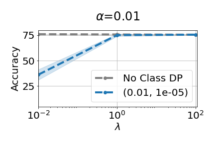
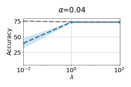
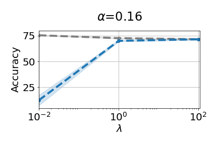
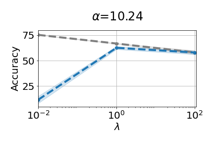
Figure 2: Accuracy vs. regularization. Server model inference accuracy of FedAUXfdp on ShuffleNet with and without $(\epsilon=0.01,\delta=1e-05)$ class model differential privacy at various levels of class model regularization $\lambda$.

Distill Data	$\alpha=0.01$	$\alpha=0.04$	$\alpha=0.16$	$\alpha=10.24$
STL-10	77.2 $\pm$ 0.5	75.4 $\pm$ 1.0	74.7 $\pm$ 0.9	74.4 $\pm$ 0.8
CIFAR-100	70.4 $\pm$ 0.7	68.9 $\pm$ 1.8	67.6 $\pm$ 1.6	68.5 $\pm$ 1.9

Table 4: FedAUXfdp server model inference accuracy on ResNet8 with distillation data sharing 9/10 classes (STL-10) versus entirely different distillation data classes (CIFAR-100).

The drop in accuracy of adding class differential privacy can be partially compensated for by increasing the regularization parameter $\lambda$ of the client models’ logistic regressions. Regularization reduces model variance and therefore the impact an individual datapoint has on the model. It thus affects the sensitivity of a differentially private mechanism as in the corollary from Chaudhuri et al. (2011), which our sensitivity theorem generalizes. As shown in Figure 2, on the ShuffleNet model architecture, increasing the regularization from $\lambda=0.01$ to $\lambda=1$ nearly eliminates the gap between the accuracy with and without $(\epsilon=0.01,\delta=10^{-5})$ class model differential privacy at all levels of data heterogeneity $\alpha$. The additional regularization does, however, reduce the accuracy of the model without the class differential privacy, moreso the more homogeneous the client data.

Table 4 shows results on ResNet with both STL-10 and CIFAR-100 as distillation data. STL-10 and CIFAR10 share 9/10 of the same classes, while CIFAR-100 has completely different classes. Even with distillation classes unmatching client classes, we still see robust results.

6 Conclusion

In this work, we have modified the FedAUX method, an augmentation of federated distillation, and made it fully differentially private. We have contributed a mechanism that privatizes respectably with little loss in model accuracy, particularly on non-iid client data. We additionally contributed a theorem for the sensitivity of $l_{2}$ regularized multinomial logistic regression. On large scale image datasets we have examined the impact of different amounts of differential privacy and regularization. Measuring the impact of federated averaging, distillation, and differential privacy on the attackability of the global server model would be an interesting investigation direction.

References

- Abadi et al. [2016] Martin Abadi, Andy Chu, Ian Goodfellow, H Brendan McMahan, Ilya Mironov, Kunal Talwar, and Li Zhang. Deep learning with differential privacy. In Proceedings of the 2016 ACM SIGSAC Conference on Computer and Communications Security (CCS), pages 308–318, 2016.
- Chang et al. [2019] Hongyan Chang, Virat Shejwalkar, Reza Shokri, and Amir Houmansadr. Cronus: Robust and heterogeneous collaborative learning with black-box knowledge transfer. arXiv preprint arXiv:1912.11279, 2019.
- Chaudhuri et al. [2011] Kamalika Chaudhuri, Claire Monteleoni, and Anand D. Sarwate. Differentially private empirical risk minimization. J. Mach. Learn. Res., 12:1069–1109, 2011.
- Chen and Chao [2020] Hong-You Chen and Wei-Lun Chao. FedDistill: Making bayesian model ensemble applicable to federated learning. arXiv preprint arXiv:2009.01974, 2020.
- Choquette-Choo et al. [2021] Christopher A. Choquette-Choo, Florian Tramer, Nicholas Carlini, and Nicolas Papernot. Label-only membership inference attacks. In Proceedings of the 38th International Conference on Machine Learning, PMLR, volume 139, pages 1964–1974, 2021.
- Dwork and Roth [2014] Cynthia Dwork and Aaron Roth. The algorithmic foundations of differential privacy. Found. Trends Theor. Comput. Sci., 9(3-4):211–407, 2014.
- Geyer et al. [2018] Robin C. Geyer, Tassilo Klein, and Moin Nabi. Differentially private federated learning: A client level perspective. arXiv preprint arXiv:1712.07557v2, 2018.
- He et al. [2016] Kaiming He, Xiangyu Zhang, Shaoqing Ren, and Jian Sun. Deep residual learning for image recognition. In Proceedings of the IEEE Conference on Computer Vision and Pattern Recognition (CVPR), pages 770–778, 2016.
- Hsu et al. [2019] Tzu-Ming Harry Hsu, Hang Qi, and Matthew Brown. Measuring the effects of non-identical data distribution for federated visual classification. arXiv preprint arXiv:1909.06335, 2019.
- Itahara et al. [2020] Sohei Itahara, Takayuki Nishio, Yusuke Koda, Masahiro Morikura, and Koji Yamamoto. Distillation-based semi-supervised federated learning for communication-efficient collaborative training with non-iid private data. arXiv preprint arXiv:2008.06180, 2020.
- Kairouz et al. [2021] Peter Kairouz, H. Brendan McMahan, Brendan Avent, Aurèlien Bellet, and Mehdi Bennis. Advances and open problems in federated learning. In Foundations and Trends in Machine Learning, volume 14, pages 1–210, 2021.
- Kasiviswanathan et al. [2008] Shiva Prasad Kasiviswanathan, Homin K. Lee, Kobbi Nissim, Sofya Raskhodnikova, and Adam Smith. What can we learn privately? In 2008 49th Annual IEEE Symposium on Foundations of Computer Science, pages 531–540, 2008.
- Li et al. [2019] Qinbin Li, Zeyi Wen, and Bingsheng He. Federated learning systems: Vision, hype and reality for data privacy and protection. arXiv preprint arXiv:1907.09693, 2019.
- Li et al. [2020] Xiang Li, Kaixuan Huang, Wenhao Yang, Shusen Wang, and Zhihua Zhang. On the convergence of FedAvg on non-iid data. In Proceedings of 8th International Conference on Learning Representations (ICLR). OpenReview.net, 2020.
- Li et al. [2021] Yiying Li, Wei Zhou, Huaimin Wang, Haibo Mi, and Timothy M Hospedales. Fedh2l: Federated learning with model and statistical heterogeneity. arXiv preprint arXiv:2101.11296, 2021.
- Lin et al. [2020] Tao Lin, Lingjing Kong, Sebastian U. Stich, and Martin Jaggi. Ensemble distillation for robust model fusion in federated learning. In Advances in Neural Information Processing Systems (NeurIPS), volume 33, 2020.
- Liu and Nocedal [1989] Dong C. Liu and Jorge Nocedal. On the limited memory BFGS method for large scale optimization. Math. Program., 45(1-3):503–528, 1989.
- McMahan et al. [2017] Brendan McMahan, Eider Moore, Daniel Ramage, Seth Hampson, and Blaise Agüera y Arcas. Communication-efficient learning of deep networks from decentralized data. In Proceedings of the 20th International Conference on Artificial Intelligence and Statistics (AISTATS), pages 1273–1282, 2017.
- McMahan et al. [2018] Brendan McMahan, Daniel Ramage, Kunal Talwar, and Li Zhang. Learning differentially private recurrent language models. In Proceedings of the 8th International Conference on Learning Representations (ICLR), 2018.
- Papernot et al. [2017] Nicolas Papernot, Martín Abadi, Úlfar Erlingsson, Ian Goodfellow, and Kunal Talwar. Semi-supervized knowledge transfer for deep learning from private training data. In Proceedings of the 5th International Conference on Learning Representations (ICLR). OpenReview.net, 2017.
- Sandler et al. [2018] Mark Sandler, Andrew G. Howard, Menglong Zhu, Andrey Zhmoginov, and Liang-Chieh Chen. MobileNetV2: Inverted residuals and linear bottlenecks. In Proceedings of the IEEE Conference on Computer Vision and Pattern Recognition (CVPR), pages 4510–4520, 2018.
- Sattler et al. [2021a] Felix Sattler, Tim Korjakow, Roman Rischke, and Wojciech Samek. Fedaux: Leveraging unlabeled auxiliary data in federated learning. In IEEE Transactions on Neural Networks and Learning Systems, 2021.
- Sattler et al. [2021b] Felix Sattler, Arturo Marban, Roman Rischke, and Wojciech Samek. Cfd: Communication-efficient federated distillation via soft-label quantization and delta coding. IEEE Trans. Netw. Sci. Eng., 2021.
- Sattler et al. [2021c] Felix Sattler, Klaus-Robert Müller, and Wojciech Samek. Clustered federated learning: Model-agnostic distributed multitask optimization under privacy constraints. IEEE Transactions on Neural Networks and Learning Systems, 32(8):3710–3722, 2021.
- Shalev-Shwartz [2007] Shai Shalev-Shwartz. Online Learning: Theory, Algorithms, and Applications. PhD thesis, Hebrew University, 2007.
- Shokri et al. [2017] Reza Shokri, Marco Stronati, Congzheng Song, and Vitaly Shmatikov. Membership inference attacks against machine learning models. In IEEE Symposium on Security and Privacy, pages 3–18, 2017.
- Sun and Lyu [2021] Lichao Sun and Lingjuan Lyu. Federated model distillation with noise-free differential privacy. In Proceedings of the Thirtieth International Joint Conference on Artificial Intelligence (IJCAI-21), 2021.
- Wang et al. [2018] Tongzhou Wang, Jun-Yan Zhu, Antonio Torralba, and Alexei A. Efros. Dataset distillation. arXiv preprint arXiv:1811.10959, 2018.
- Zhang et al. [2018] Xiangyu Zhang, Xinyu Zhou, Mengxiao Lin, and Jian Sun. ShuffleNet: An extremely efficient convolutional neural network for mobile devices. In Proceedings of the IEEE Conference on Computer Vision and Pattern Recognition (CVPR), pages 6848–6856, 2018.
- Zhou et al. [2021] Yanlin Zhou, George Pu, Xiyao Ma, Xiaolin Li, and Dapeng Wu. Distilled one-shot federated learning. arXiv preprint arXiv:2009.07999, 2021.