Daisy Bloom Filters

Abstract

Weighted Bloom filters (Bruck, Gao and Jiang, ISIT 2006) are Bloom filters that adapt the number of hash functions according to the query element. That is, they use a sequence of hash functions $h_{1},h_{2},\dots$ and insert $x$ by setting the bits in $k_{x}$ positions $h_{1}(x),h_{2}(x),\dots,h_{k_{x}}(x)$ to 1, where the parameter $k_{x}$ depends on $x$. Similarly, a query for $x$ checks whether the bits at positions $h_{1}(x),h_{2}(x),\dots,h_{k_{x}}(x)$ contain a $0$ (in which case we know that $x$ was not inserted), or contains only $1$s (in which case $x$ may have been inserted, but it could also be a false positive).

In this paper, we determine a near-optimal choice of the parameters $k_{x}$ in a model where $n$ elements are inserted independently from a probability distribution $\mathcal{P}$ and query elements are chosen from a probability distribution $\mathcal{Q}$, under a bound on the false positive probability $F$. In contrast, the parameter choice of Bruck et al., as well as follow-up work by Wang et al., does not guarantee a nontrivial bound on the false positive rate. We refer to our parameterization of the weighted Bloom filter as a Daisy Bloom filter.

Standard Bloom filters use $k_{x}=\lceil\log_{2}(1/F)\rceil$ for all $x$, which leads to a space usage of $\log_{2}(e)n\log(1/F)+O(n)$ bits. For many distributions $\mathcal{P}$ and $\mathcal{Q}$, the Daisy Bloom filter space usage is significantly smaller than this. Our upper bound is complemented with an information-theoretical lower bound, showing that (with mild restrictions on the distributions $\mathcal{P}$ and $\mathcal{Q}$), the space usage of Daisy Bloom filters is the best possible up to a constant factor. This improves a previous, non-tight lower bound of Wang et al.

Daisy Bloom filters can be seen as a fine-grained variant of a recent data structure of Vaidya, Knorr, Mitzenmacher and Kraska that uses several (“partitioned”) Bloom filters to handle different, carefully chosen subsets of the universe $\mathcal{U}$ with different false positive rates. Like their work, we are motivated by settings in which we have prior knowledge of the workload of the filter, possibly in the form of advice from a machine learning algorithm.

1 Introduction

The Bloom filter [4] is a widely used data structure for storing an approximation of a given set $S$ of elements from some universe $\mathcal{U}$ (a countable set). It represents a superset $S^{\prime}\supseteq S$ that is “close to $S$” in the sense that for $x\not\in S$, the probability that $x\in S^{\prime}$ is bounded by some $F>0$. The parameter $F$ is referred to as the false positive probability. The advantage of using a Bloom filter, when some false positives are acceptable, is that the space usage becomes smaller than what is required to store $S$ exactly.

Though the space usage of Bloom filters is known to be within a small constant factor from optimal from a worst-case perspective [8], it is clear that they may not be close to optimal for particular distributions of data and queries. Suppose that we care only about the total fraction of false positives for a sequence of queries, rather than the false positive probability of each individual query. This is reasonable in many applications of Bloom filters, for example in network applications where the cost of a false positive may be sending a request for data associated with a key $x$ to a server that does not contain this data [5]. Now suppose that some elements are in $S$ with probability close to 1. Then it would make sense to always include them in $S^{\prime}$, saving space by not having to represent these elements in the filter [16]. More generally, as pointed out already by Bruck, Gao and Jiang [6], we can consider the false positive probability not just over the random choices of the data structure, but also over the query distribution.

Recently, several papers [9, 16, 19, 25] considered Bloom filters in settings with advice. The advice could, for example, be knowledge about the a priori probability $p_{x}$ that an element $x$ is in the set $S$. Such advice might be provided by a machine learning algorithm or statistical information from past data. Vaidya, Knorr, Mitzenmacher, and Kraska [25] show that it is advantageous to treat elements differently depending on such advice. Specifically, they split $\mathcal{U}$ into subsets $\mathcal{U}_{1},\mathcal{U}_{2},\dots$ and build a Bloom filter for each. They show how to find the best false positive probabilities for each Bloom filter, depending on the sizes of $\mathcal{U}_{i}$, $\mathcal{U}_{i}\cap S$ as well as the fraction of queries in each $\mathcal{U}_{i}$, such that the total number of false positives is bounded. While the existence of a query distribution is implicitly assumed in Vaidya et al. [25], a theoretical advantage of our work is that it makes the influence of the query distribution to the design of the filter explicit. In particular, it is somewhat surprising that when $p_{x}=q_{x}$, we cannot hope to do better than the standard Bloom filter.

Our contribution is two-fold:

• First, we revisit the weighted Bloom filter construction of Bruck et al. [6] which adjusts the false positive rate by varying the number of hash functions used for each element, avoiding partitioning of the set into several data structures. It turns out that a near-optimal choice of false positive rate for each element $x$, minimizing space while ensuring false positive rate $F$, depends only on $p_{x}$, the query probability $q_{x}$, and the expected size $n$ of the set $S$. In contrast, the parameter choices of [6, 26] yield a trivial false positive rate of 1 for some query distributions.

• Second, we formalize a natural randomized generative model of data and queries (similar to the one used in [6]), and show that Daisy Bloom filters are information-theoretically space-optimal, up to a constant factor, in this model. Our lower bound uses an encoding argument that generalizes space lower bounds for standard Bloom filters (which hold for uniformly random sets and queries). This improves a non-tight “approximate lower bound” shown by Wang et al. [26].

We name our variant of the weighted Bloom filter a Daisy Bloom filter. The daisy is one of our favorite flowers, especially when in full bloom, and it is also the nickname of the Danish queen, whose residence is not far from the place where this work was conceived. Finally, it is a subsequence of “dynamic strechy” which describes the key properties of our data structure. Specifically, our construction is dynamic in that, as opposed to the one in Vaidya et al. [25], it does not require us to know the input set in advance (in particular, it supports insertions). Additionally, it is stretchy in that the number of hash functions $k_{x}$ we employ for each element $x$ varies and is always upper bounded in the worst case by $\lceil\log_{2}(1/F)\rceil$.

The model. We let $\mathcal{P}$ and $\mathcal{Q}$ denote two distributions over $\mathcal{U}$ and let $p_{x}$ (and $q_{x}$, respectively) denote the probability of drawing a specific element $x\in\mathcal{U}$ from $\mathcal{P}$ (and $\mathcal{Q}$, respectively). The input set is generated by $n$ independent draws (with replacement) from $\mathcal{P}$ and then inserted into the filter. We refer to the product distribution induced by these $n$ draws as the input distribution $\mathcal{P}_{n}$. Similarly, we refer to $\mathcal{Q}$ as the query distribution.

The filter. Let $A$ denote the filter and let $A(S,x)\in\left\{\textsf{YES},\textsf{NO}\right\}$ denote the output of $A$ when queried on an element $x\in\mathcal{U}$, after having been given a set $S\subseteq\mathcal{U}$ as input. For a fixed input set $S$, the probability that a filter answers YES on a given query only depends on its internal randomness. We then say that $A$ is a $Q$-filter with false positive rate $0<F<1$ on $S$ if it satisfies the following conditions:

1. No false negatives: For all $x\in S$, we have that ${\mathrm{Pr}}\left[A(S,x)=\textsf{YES}\right]=1$

2. Bounded false positive rate:

   $$\sum_{x\in\mathcal{U}\setminus S}q_{x}\cdot{\mathrm{Pr}}\left[A(S,x)=\textsf{YES}\right]\leq F\;.$$

Note that the above false positive rate is defined as the average false positive probability over the distribution $Q$ on the queries. We require that it is at most $F$ for any set $S$ (and not on average over all sets $S$) and we show a construction that achieves this guarantee for all but a subset of (bad) input sets that occur with low probability in $\mathcal{P}_{n}$.

1.1 Our Contributions

In this paper, we consider the problem of designing filters in the generalized context in which the input set comes from a (product) distribution $\mathcal{P}_{n}$ and the false positive rate is computed with respect to a query distribution $\mathcal{Q}$. We give both lower and upper bounds for the space that such a $\mathcal{Q}$-filter on $\mathcal{P}_{n}$ requires.

Theorem 1.1 (informal).

Let $\mathcal{P}_{n}$ and $Q$ be defined as above. Given $0<F<1$, the Daisy Bloom filter is a $\mathcal{Q}$-filter with the following guarantees:

• it has a false positive rate at most $F$ with high probability over $\mathcal{P}_{n}$, whenever $\mathcal{P}$ and $Q$ satisfy $\sum_{x\in\mathcal{U}}p_{x}q_{x}\leq F/n$,

• the time it takes to perform queries and insertions is at most $\log_{2}(1/F)$ in the worst case,

• the space it requires is within a $\log_{2}(e)$ multiplicative factor and a low order linear term of the lower bound on the expected size of any $\mathcal{Q}$-filter with false positive rate at most $F$ for sets from $\mathcal{P}_{n}$.

We defer the explicit formulation of the space bounds to Section 3 (upper bound) and Section 5 (lower bound) and note here that they show exact dependencies on $p_{x}$ and $q_{x}$ (versus Vaidya et al. [25]). In particular, they show that, when $\mathcal{P}=\mathcal{Q}$, the Daisy Bloom filter degenerates into a regular Bloom filter and that this is tight (with respect to Bloom filters). Moreover, the running time of each operation is at most $\log_{2}(1/F)$ in the worst case (in contrast to Bruck et al. [6] and Wang et al. [26]). Finally, our false positive probability guarantee holds with high probability over the choice of the input set, as long as $\sum_{x\in\mathcal{U}}p_{x}q_{x}\leq F/n$. This condition can be seen as a generalized version of the standard filter assumption that $\left|\mathcal{U}\right|\geq n/F$, where $\left|\mathcal{U}\right|$ denotes the size of the universe (i.e., consider the uniform distributions $q_{x}=p_{x}=1/\left|\mathcal{U}\right|$). For such small values of $F<n/\left|\mathcal{U}\right|$, standard filters essentially has to answer correctly on all queries and the lower bound of $n\log_{2}(1/F)-O(1)$ does not hold [8, 10].

In terms of the lower bound, previous approaches for filters [8, 10] show that there exists a set $S\subseteq U$ of size $n$ for which the filter needs to use $n\log_{2}(1/F)-O(1)$ bits. This type of lower bound is still true in our model but it does not necessarily say anything meaningful, since the bad set $S$ could be sampled in $\mathcal{P}_{n}$ with a negligible probability. In our model, it is therefore more natural to lower bound the expected size of the filter over the randomness of the input set. We show that this lower bound holds even when the filter has false positive rate at most $F$ for all but an unlikely collection of possible input sets (see Theorem 5.1).

1.2 Previous Work

Filters have been studied extensively in the literature [1, 2, 3, 8, 10, 17, 20, 21, 22], with Bloom filters perhaps the most widely employed variants in practice [18]. Learning-based approaches to classic algorithm design have recently attracted a great deal of attention, see e.g. [11, 14, 15, 16, 23].

Weighted Bloom Filters. Bruck, Gao and Jiang [6] explored the idea of letting the number $k_{x}$ of hash functions used depend on the element being inserted or queried. That is, they use a sequence of hash functions $h_{1},h_{2},\dots$ and insert $x$ by setting the bits in $k_{x}$ positions $h_{1}(x),h_{2}(x),\dots,h_{k_{x}}(x)$ to 1, where the parameter $k_{x}$ depends on $x$. Similarly, a query for $x$ checks whether the bits at positions $h_{1}(x),h_{2}(x),\dots,h_{k_{x}}(x)$ contain a $0$ (in which case we know that $x$ was not inserted), or contains only $1$s (in which case $x$ may have been inserted, but it could also be a false positive).

Given information about the probability of inserting and querying each element, they set out to find an optimal choice of the parameters $k_{x}$ thats limit the false positive rate (in expectation over both the input and the query distribution). The approach is to solve an unconstrained optimization problem where the variables $k_{x}$ can be any real number. In a post-processing step each $k_{x}$ is rounded to the nearest non-negative integer. Unfortunately this process does not lead to an optimal choice of parameters, and in fact does not guaranteed a non-trivial false positive rate. The issue is that the solution to the unconstrained problem may have many negative values of $k_{x}$, so even though the weighted sum $\sum_{x}p_{x}k_{x}$ is bounded, the post-processed sum $\sum_{x}p_{x}\max(k_{x},0)$ can be arbitrarily large. In particular, this is the case if at least one element is queried very rarely. This means that the weighted Bloom filter may consist only of 1s with high probability, resulting in a false positive probability of 1.

Wang, Ji, Dang, Zheng and Zhao [26] noticed that there is a mistake in [6] that leads them to compute suboptimal values for $k_{x}$. They attempt to correct the values for $k_{x}$, but their analysis still suffers from the same, more fundamental, problem: the existence of a very rare query element drives the false positive rate to 1. Wang et al. [26] also show an information-theoretical “approximate lower bound” on the number of bits needed for a weighted Bloom filter with given distributions $\mathcal{P}$ and $\mathcal{Q}$. The sense in which the lower bound is approximate is not made precise, and the lower bound is certainly not tight (for example, it can be negative).

Partitioned Learned Bloom Filters. In the work of Vaidya, Knorr, Mitzenmacher and Kraska [25], the data structure has access to a learned model of the input set. The model is given a fixed input set $S$ and a representative sample of elements in $\mathcal{U}\setminus S$, where the sample is representative with respect to some query distribution. Given a query element $x$, the model returns a score $s(x)\in[0,1]$, which can be intuitively thought of as the model’s belief that $x\in S$.

Vaidya et al. [25] then consider a specific filter design based on choosing a fixed number of $k$ thresholds $0=\tau_{0}\leq\tau_{1}\leq\ldots\leq\tau_{k}=1$, partitioning the elements according to these thresholds, and building separate Bloom filters for each class of the partition. Specifically, let $\mathcal{U}_{i}\triangleq\left\{x\in\mathcal{U}|s(x)\in[\tau_{i},\tau_{i+1}]\right\}$ be the set of elements whose scores fall in the range $[\tau_{i},\tau_{i+1}]$ and let $f_{i}\in[0,1]$ be the false positive error of the $i^{\text{th}}$ filter. Then the space of the data structure is proportional to $\sum_{i}\left|S_{i}\right|\log(1/f_{i})$, where $S_{i}=S\cap\mathcal{U}_{i}$, and the overall false positive rate is computed as $\sum_{i}H_{i}\cdot f_{i}$, where $H_{i}$ denotes the probability that a query element $x\notin\mathcal{U}\setminus S$ is in $\mathcal{U}_{i}\setminus S_{i}$.

Given some threshold values, Vaidya et al. [25] then formulate the optimization problem of setting the false positive rates $f_{i}$ such that the total space of the data structure is minimized and the overall false positive rate is at most a given $F$. In the relaxed version in which each $f_{i}$ is allowed to be greater than $1$, they obtain exact optimal values for $f_{i}=F\cdot(\left|S_{i}\right|/\left|S\right|)/H_{i}$. To put this quantity in perspective, consider the case in which each element in $\mathcal{U}\setminus S$ is equally likely to be queried. Then $H_{i}=\left|U_{i}\setminus S_{i}\right|/\left|U\setminus S\right|$ and $f_{i}$ becomes proportional to the ratio $\left|S_{i}\right|/\left|\mathcal{U}_{i}\setminus S_{i}\right|$ of keys to non-keys within $\mathcal{U}_{i}$. For a more detailed comparison on how the shape of the score and the false positive rates $f_{i}$ compare to the design of the Daisy Bloom filter, we refer the reader to Appendix A.

1.3 Paper Organization

After some preliminaries, Sections 3 and 4 present the Daisy Bloom filter and its analysis. Section 5 shows our lower bound on the space usage, matching the upper bound up to a constant factor for most parameters.

2 Preliminaries

Notation. We refer to the product distribution induced by the $n$ independent draws from $\mathcal{P}$ as $\mathcal{P}_{n}$. For clarity, throughout the paper, we will distinguish between probabilities over the randomness of the input set, denoted by $\mathrm{Pr}_{\mathcal{P}_{n}}\left[\cdot\right]$, and probabilities over the internal randomness of the filter, denoted by $\mathrm{Pr}_{A}\left[\cdot\right]$. Joint probabilities are denoted by $\mathrm{Pr}_{\mathcal{P}_{n},A}\left[\cdot\right]$.

With high probability guarantees. The high probability guarantees we obtain are of the form $1-\exp\left(-\Theta(\textsf{LB}(\mathcal{P}_{n},\mathcal{Q},F)/\log^{O(1)}(1/F))\right)$, where $\textsf{LB}(\mathcal{P}_{n},\mathcal{Q},F)-O(n)$ is the lower bound we obtain for the space of $Q$-filters with false positive rate $F$ on sets in $\mathcal{P}_{n}$ (see Section 3 for a formal definition). Clearly, such bounds are meaningful for distributions in which the optimal size $\textsf{LB}(\mathcal{P}_{n},\mathcal{Q},F)$ of a filter is not too small. Similarly, we can assume that the size of the universe is polynomial in $n$, and so $\log(1/F)=O(\log(n))$ in the standard case in which $F>n/\left|\mathcal{U}\right|$. Therefore, while in general $\textsf{LB}(\mathcal{P}_{n},\mathcal{Q},F)$ can be much smaller than $n\log_{2}(1/F)$, we do require some mild dependency on $n$ in order for the high probability bounds to be meaningful.

Access to $\mathcal{P}$ and $\mathcal{Q}$. For simplicity, we present our results assuming access to an oracle that retrieves $p_{x}$ and $q_{x}$ in constant time for any $x\in\mathcal{U}$. However, our analysis follows through even if we have a constant factor approximation for $p_{x}$ and $q_{x}$, in the sense in which the space of the filter increases by $O(n)$ bits and the time to perform each operation by an added constant. The assumption of access to such an approximate oracle is standard [7, 13] and can be based on samples of historical information, on statistics such as histograms, or on machine learning models (see for instance, the neural-net based frequency predictor of Hsu et al. [15]). We do not account for the cost of training in the space and time bounds of our filter and note that training can be done just once in a pre-processing phase, since the design of our filter is independent of the actual realisation of the input set.

Kraft’s inequality. For the lower bound, we make us of the following classic result in data compression:

Theorem 2.1 (Kraft’s inequality [24]).

For any instantaneous code (prefix code) over an alphabet of size $D$, the codeword lengths $\ell_{1},\ell_{2},\ldots,\ell_{m}$ must satisfy the inequality

$$\sum_{i}D^{-\ell_{i}}\leq 1\;.$$

Conversely, given a set of codeword lengths that satisfy this inequality, there exists an instantaneous code with these word lengths.

3 The Daisy Bloom Filter

We parametrize a Daisy Bloom filter construction as a function of $\mathcal{P}_{n},\mathcal{Q}$ and $F$ and refer to it as a $(\mathcal{P}_{n},\mathcal{Q},F)$ Daisy Bloom filter. We define the number $k_{x}$ of hash functions that an element $x$ employs as such:

$$k_{x} \triangleq\begin{cases}0&\text{if $q_{x}\leq Fp_{x}$ or $p_{x}>1/n$}\;,\\ \log(1/F\cdot q_{x}/p_{x})&\text{if $Fp_{x}<q_{x}\leq\min\!\left\{p_{x},F/n\right\}$}\;,\\ \log(1/F)&\text{if $q_{x}>p_{x}$ and $F/n\geq p_{x}$}\;,\\ \log(1/(np_{x}))&\text{if $q_{x}>F/n$ and $F/n<p_{x}\leq 1/n$}\;.\end{cases}$$

Intuitively the first case covers the situation where $x$ is queried very rarely, or is a true positive with constant probability, so that it does not pay to store any information about it. Thus we set $k_{x}=0$ which means that we always include $x$ in the set $S^{\prime}$ of positives. The third case intuitively covers the case where $x$ is queried so often that we need to keep the false positive probability below $F$, which is achieved by setting $k_{x}=\log(1/F)$. The fourth case interpolates between the first and third case for elements that are not too rarely queried, in which case the precise query probability does not matter. Similarly, the second case interpolates smoothly between the first and third cases for elements that are rarely (but not very rarely) queried. See also Figure 1 for visualization of the different regimes.

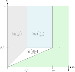
Figure 1: A schematic visualization of the different regimes for $k_{x}$.

The definition of $k_{x}$ clearly defines a partition of the universe into 4 parts. For the analysis, it will make sense to further partition one of these and consider 5 parts.

$$\mathcal{U}_{0} \triangleq\left\{x\in\mathcal{U}\mid q_{x}\leq Fp_{x}\right\}\;,$$

$$\mathcal{U}_{1} \triangleq\left\{x\in\mathcal{U}\mid q_{x}>Fp_{x}\text{ and }p_{x}>1/n\right\}\;,$$

$$\mathcal{U}_{2} \triangleq\left\{x\in\mathcal{U}\mid Fp_{x}<q_{x}\leq\min\!\left\{p_{x},F/n\right\}\right\}\;,$$

$$\mathcal{U}_{3} \triangleq\left\{x\in\mathcal{U}\mid q_{x}>p_{x}\text{ and }F/n\geq p_{x}\right\}\;,$$

$$\mathcal{U}_{4} \triangleq\left\{x\in\mathcal{U}\mid q_{x}>F/n\text{ and }F/n<p_{x}\leq 1/n\right\}\;.$$

We then define the term

$$\textsf{LB}(\mathcal{P}_{n},\mathcal{Q},F) =n\cdot\left(\sum_{x\in\mathcal{U}_{2}}p_{x}\log(1/F\cdot q_{x}/p_{x})+\sum_{x\in\mathcal{U}_{3}}p_{x}\log(1/F)+\sum_{x\in\mathcal{U}_{4}}p_{x}\log(1/(np_{x}))\right)\;.$$

Let $X_{i}$ denote the number of hash functions that are employed when we sample in the $i^{th}$ round, i.e., $X_{i}=k_{x}$ with probability $p_{x}$. Then $X=\sum_{i}X_{i}$ denotes the number of locations that are set in the Bloom filter (where the same location might be set multiple times). Moreover, $\mathbb{E}_{\mathcal{P}_{n}}\left[X\right]=n\cdot\sum_{x\in\mathcal{U}}p_{x}k_{x}=\textsf{LB}(\mathcal{P}_{n},\mathcal{Q},F)$, since the $\left\{X_{i}\right\}_{i}$ are identically distributed. Finally, we set the length $\textsf{DB}(\mathcal{P}_{n},\mathcal{Q},F)$ of the Daisy Bloom filter array to

$$\textsf{DB}(\mathcal{P}_{n},\mathcal{Q},F)\triangleq\log(e)\cdot\textsf{LB}(\mathcal{P}_{n},\mathcal{Q},F/6).$$

The two main theorems of the paper is the following upper and lower bound.

Theorem 3.1 (Upper bound).

There exists $\mathcal{T}\subseteq\mathbb{P}(U)$ such that $S\in\mathcal{T}$ with high probability over the randomness of $\mathcal{P}_{n}$, and for all $S\in\mathcal{T}$ the Daisy Bloom Filter is a $\mathcal{Q}$-filter for $S$ with false positive rate at most $F$. The Daisy Bloom filter uses $\textsf{DB}(\mathcal{P}_{n},\mathcal{Q},F)=\log(e)\cdot\textsf{LB}(\mathcal{P}_{n},\mathcal{Q},F/6)=\log(e)\cdot\textsf{LB}(\mathcal{P}_{n},\mathcal{Q},F)+O(n)$ bits.

The sets in $\mathcal{T}$ are the sets for which $X\approx\mathbb{E}_{\mathcal{P}_{n}}\left[X\right]=\textsf{LB}(\mathcal{P}_{n},\mathcal{Q}_{F})$. The reason, we constraint ourself to these sets, is that if $X\gg\textsf{LB}(\mathcal{P}_{n},\mathcal{Q}_{F})$ then most bits will be set to 1 which will make the false positive rate large. We will bound the probability that $X\gg\textsf{LB}(\mathcal{P}_{n},\mathcal{Q}_{F})$ by using Bernstein’s inequality and here it becomes a crucial fact that we know that $k_{x}\leq\log(1/F)$.

Theorem 3.2 (Lower bound).

Let $A$ be an algorithm and assume that for any input set $S\subseteq\mathcal{U}$ with $\left|S\right|\leq n$, $A(S)$ is a $Q$-filter for $S$ with false positive rate at most $F$. Then the expected size of $A(S)$ must satisfy

$$\mathbb{E}_{\mathcal{P}_{n},A}\left[\left|A(S)\right|\right]\geq\textsf{LB}(\mathcal{P}_{n},\mathcal{Q},F)-1-6n\;,$$

where $S$ is sampled with respect to $\mathcal{P}_{n}$.

Remark 3.3.

The lower bound we prove is actually slightly stronger. We only require that $A(S)$ is a $Q$-filter for $S$ with false positive rate at most $F$ for $S\in\mathcal{T}$ where $\mathcal{T}\subseteq\mathbb{P}(U)$ and $\mathrm{Pr}_{\mathcal{P}_{n}}\left[S\not\in\mathcal{T}\right]\leq\frac{1}{\log u}$.

4 Upper Bound

We now show that the above construction is a $(\mathcal{P}_{n},\mathcal{Q})$ filter with a false positive rate $\Theta(F)$. In the following, we employ the notation $m\triangleq\mathbb{E}_{\mathcal{P}_{n}}\left[X\right]/\ln 2$ for readability.

We first show that $X$ is tightly concentrated around its expectation. For this we first need the following observation. For every $x\in\mathcal{U}$, $k_{x}\leq\log(1/F)$.

Proof 4.1.

For $x\in\mathcal{U}_{0}\cup\mathcal{U}_{1}$, we have that $k_{x}=0$ which is clearly less than $\log(1/F)$. For $x\in\mathcal{U}_{3}$ we have that $k_{x}=\log(1/F)$ and again the statement holds trivially. For $x\in\mathcal{U}_{2}$, we have that $q_{x}\leq p_{x}$ and so $k_{x}=\log(1/F\cdot q_{x}/p_{x})\leq\log(1/F)$. For $x\in\mathcal{U}_{4}$, we have that $p_{x}>F/n$ and so $k_{x}=\log(1/(np_{x}))<\log(1/F)$.

We are now ready to prove that the random variable $X$ is concentrated around its expectation.

Lemma 4.2.

For any $\delta>0$,

$$\mathrm{Pr}_{\mathcal{P}_{n}}\left[X>(1+\tau)\cdot\mathbb{E}_{\mathcal{P}_{n}}\left[X\right]\right] \leq\exp\left(-\frac{\tau^{2}\ln 2}{2(1+\tau/3)}\cdot\frac{m}{\log(1/F)}\right)$$

Proof 4.3.

The random variables $\left\{X_{i}\right\}_{i}$ are independent and $X_{i}\leq b\triangleq\log(1/F)$ for all $i$ by Obs. 4. We apply Bernstein’s inequality (see Appendix C):

$$\mathrm{Pr}_{\mathcal{P}_{n}}\left[X-\mathbb{E}_{\mathcal{P}_{n}}\left[X\right]>t\right]\leq\exp\left(-\frac{t^{2}/2}{n\text{Var}_{\mathcal{P}_{n}}\left[X_{1}\right]+bt/3}\right)\;.$$

Note that $\text{Var}_{\mathcal{P}_{n}}\left[X_{i}\right]\leq\mathbb{E}_{\mathcal{P}_{n}}\left[X_{i}^{2}\right]\leq b\cdot\mathbb{E}_{\mathcal{P}_{n}}\left[X_{i}\right]$. Setting $t=\tau\cdot\mathbb{E}_{\mathcal{P}_{n}}\left[X\right]=\tau n\cdot\mathbb{E}_{\mathcal{P}_{n}}\left[X_{1}\right]$, we get that

$$\mathrm{Pr}_{\mathcal{P}_{n}}\left[X>(1+\tau)\mathbb{E}_{\mathcal{P}_{n}}\left[X\right]\right] \leq\exp\left(-\frac{\tau^{2}}{2}\cdot\frac{n^{2}(\mathbb{E}_{\mathcal{P}_{n}}\left[X_{1}\right])^{2}}{nb\cdot\mathbb{E}_{\mathcal{P}_{n}}\left[X_{1}\right]+\tau/3\cdot nb\cdot\mathbb{E}_{\mathcal{P}_{n}}\left[X_{1}\right]}\right)$$

$$=\exp\left(-\frac{\tau^{2}}{2(1+\tau/3)}\cdot\frac{n\mathbb{E}_{\mathcal{P}_{n}}\left[X_{1}\right]}{b}\right)\;.$$

The claim follows by noticing that $n\mathbb{E}_{\mathcal{P}_{n}}\left[X_{1}\right]=m\ln 2$.

We will now prove that as long as $X\leq(1+1/(2\log(1/F)))\mathbb{E}_{\mathcal{P}_{n}}\left[X\right]$ then the Daisy Bloom filter is a $\mathcal{Q}$-filter on $S$ with false positive rate $6F$. Thus combining this with Lemma 4.2 we get that with probability $1-\exp\left(-\frac{m}{\Theta(\log^{3}(1/F))}\right)$ over the randomness of the input set, the Daisy Bloom filter is a $\mathcal{Q}$-filter on $S$ with false positive rate $6F$. This is exactly the statement of Theorem 3.1.

Lemma 4.4.

Assume that $\mathcal{P}_{n}$ and $\mathcal{Q}$ satisfy $n\sum_{x\in\mathcal{U}}p_{x}q_{x}\leq F$, and that $X\leq(1+1/(2\log(1/F)))\mathbb{E}_{\mathcal{P}_{n}}\left[X\right]$. Then the Daisy Bloom filter is a $\mathcal{Q}$-filter on $S$ with false positive rate of at most $6F$.

Proof 4.5.

Let $\rho\in[0,1]$ denote the fraction of entries in the Bloom filter that are set to $0$ after we have inserted the elements of the set. We first show that $\rho$ is close to $1/2$ with high probability over the input set and over the randomness of the hash functions. Recall that the random variable $X$ denotes the total number of entries that are set in the Bloom filter, including multiplicities. In the worst case, all the entries to the filter are distinct, and we have $X$ independent chances to set a specific bit to $1$. Therefore

$$\mathbb{E}_{h}\left[\rho|X\right]\geq\left(1-\frac{1}{m}\right)^{X}\approx e^{-X/m}=2^{-X/\mathbb{E}_{\mathcal{P}_{n}}\left[X\right]}\;.$$

Moreover, by applying a Chernoff bound for negatively associated random variables, we have that for any $0<\gamma<1$,

$$\mathrm{Pr}_{A}\left[\rho\leq(1-\gamma)\cdot\left(1-\frac{1}{m}\right)^{X}\,\middle|\,X\right] \leq\exp\left(-m\left(1-\frac{1}{m}\right)^{X}\cdot\gamma^{2}/2\right)$$ (1)

We now let $B_{\delta}$ denote the event that $\left(1-\frac{1}{m}\right)^{X}>(1-\delta)\cdot\frac{1}{2}$ and $B_{\gamma}$ the event that $\rho>(1-\gamma)\left(1-\frac{1}{m}\right)^{X}$. We then choose $0<\delta<1$ and $0<\gamma<1$ such that $B_{\delta}$ and $B_{\delta^{\prime}}$ imply that

$$\rho\geq 1-2^{1/\log(1/F)}\cdot\frac{1}{2}\;.$$

Moreover, for our choices of $\delta$ and $\gamma$, we have that both $B_{\delta}$ and $B_{\gamma}|B_{\delta}$ occur with high probability. See Appendix B for technical details. Conditioned on $B_{\delta}$ and $B_{\gamma}$, we get that, for an $x\notin S$, since $k_{x}\leq\log(1/F)$,

$$\mathrm{Pr}_{A}\left[A(S,x)=\textsf{YES}|B_{\delta}\wedge B_{\gamma}\right]=(1-\rho)^{k_{x}}\leq 2^{k_{x}/b}\cdot 2^{-k_{x}}\leq 2\cdot 2^{-k_{x}}$$

We bound the false positive rate on each partition. For $x\in\mathcal{U}_{0}$, i.e., with $q_{x}\leq Fp_{x}$ and $k_{x}=0$, we can upper bound the false positive rate as such

$$\sum_{x\in\mathcal{U}_{0}}q_{x}\cdot{\mathrm{Pr}}\left[A(S,x)=\textsf{YES}|B_{\delta}\wedge B_{\gamma}\right] \leq\sum_{x\in\mathcal{U}_{0}}q_{x}\leq\sum_{x\in\mathcal{U}_{0}}p_{x}\cdot F\;.$$

For $x\in\mathcal{U}_{1}$ with $p_{x}>1/n$ and $k_{x}=0$, we have the following

$$\sum_{x\in\mathcal{U}_{1}}q_{x}\cdot{\mathrm{Pr}}\left[A(S,x)=\textsf{YES}|B_{\delta}\wedge B_{\gamma}\right] \leq\sum_{x\in\mathcal{U}_{1}}q_{x}<n\sum_{x\in\mathcal{U}_{1}}p_{x}q_{x}\;.$$

For $x\in\mathcal{U}_{2}$ with $k_{x}=\log(1/F\cdot q_{x}/p_{x})$, we have the following

$$\sum_{x\in\mathcal{U}_{2}}q_{x}\cdot{\mathrm{Pr}}\left[A(S,x)=\textsf{YES}|B_{\delta}\wedge B_{\gamma}\right] \leq\sum_{x\in\mathcal{U}_{2}}q_{x}\cdot 2\cdot 2^{-k_{x}}=\sum_{x\in\mathcal{U}_{2}}q_{x}\cdot 2\cdot p_{x}/q_{x}\cdot F$$

$$=\sum_{x\in\mathcal{U}_{2}}p_{x}\cdot 2F\;.$$

For $x\in\mathcal{U}_{3}$ with $k_{x}=\log(1/F)$,

$$\sum_{x\in\mathcal{U}_{3}}q_{x}\cdot{\mathrm{Pr}}\left[A(S,x)=\textsf{YES}|B_{\delta}\wedge B_{\gamma}\right] \leq\sum_{x\in\mathcal{U}_{3}}q_{x}\cdot 2F\leq 2F\;.$$

For $x\in\mathcal{U}_{4}$ with $k_{x}=\log(1/(np_{x}))$,

$$\sum_{x\in\mathcal{U}_{4}}q_{x}\cdot{\mathrm{Pr}}\left[A(S,x)=\textsf{YES}|B_{\delta}\wedge B_{\gamma}\right] \leq\sum_{x\in\mathcal{U}_{4}}q_{x}\cdot 2nP_{x}\leq 2n\sum_{x\in\mathcal{U}_{4}}p_{x}q_{x}\;.$$

For the overall false positive rate, note that the total false positive rate in $\mathcal{U}_{0}$ and $\mathcal{U}_{2}$ is at most $2F$. Similarly for the false positive rate in $\mathcal{U}_{3}$. For the remaining partitions $\mathcal{U}_{2}$ and $\mathcal{U}_{4}$, we have that it is at most

$$2n\sum_{x\in\mathcal{U}_{1}\cup\mathcal{U}_{4}}p_{x}q_{x}\;.$$

From our assumption, this later term is at most $2F$ as well.

5 The Lower Bound

The goal of this section is to prove Theorem 3.2. As discussed we prove a slightly stronger statement where we allow our algorithm to not produce a $Q$-filter for some of the set $S$ as long as the probability of sampling them are low.

Theorem 5.1.

Let $\mathcal{T}\subseteq\mathbb{P}(\mathcal{U})$ be given such that $\mathrm{Pr}_{\mathcal{P}_{n}}\left[S\not\in\mathcal{T}\right]\leq\frac{1}{\log u}$. If $A$ is an algorithm such that for all $S\in\mathcal{T}$, $A(S)$ is a $Q$-filter for $S$ with false positive rate at most $F$. Then the expected size of $A(S)$ must satisfy

$$\mathbb{E}_{\mathcal{P}_{n},A}\left[\left|A(S)\right|\right]\geq\textsf{LB}(\mathcal{P}_{n},\mathcal{Q},F)-1-6n\;,$$

where $S$ is sampled with respect to $\mathcal{P}_{n}$.

Proof 5.2.

Each instance $\mathcal{I}$ of the data structure corresponds to a subset $\mathcal{U}_{\mathcal{I}}\subset\mathcal{U}$ on which the data structure answers YES. We denote the number of bits needed by such an instance by $\left|\mathcal{I}\right|$. For any set $S\in\mathcal{T}$, we have that $\mathcal{I}=A(S)$ satisfies that $S\subseteq\mathcal{U}_{\mathcal{I}}$ and

$$\mathbb{E}_{A}\left[\sum_{x\in\mathcal{U}_{\mathcal{I}}\setminus S}q_{x}\right]\leq F\;.$$

The goal is to prove that

$$\mathbb{E}_{\mathcal{P}_{n},A}\left[\left|A(S)\right|\right]\geq n\cdot\left(\sum_{x\in\mathcal{U}_{2}}p_{x}\log(1/F\cdot q_{x}/p_{x})+\sum_{x\in\mathcal{U}_{3}}p_{x}\log(1/F)+\sum_{x\in\mathcal{U}_{4}}p_{x}\log(1/(np_{x}))\right)-1-6n\;.$$

We will lower bound $\mathbb{E}_{\mathcal{P}_{n},A}\left[\left|A(S)\right|\right]$ by using it to encode an ordered sequence of $n$ elements drawn according to $\mathcal{P}_{n}$. Specifically, for any ordered sequence of $n$ elements $\hat{S}\in\mathcal{U}^{n}$, we let $S\subseteq U$ be the set of distinct elements and let $\mathcal{I}=A(S)$ as above. We first note that to encode $\hat{S}\sim\mathcal{P}_{n}$ then in expectation we need at least the entropy number of bits, i.e.,

$$n\sum_{x\in\mathcal{U}}p_{x}\log\tfrac{1}{p_{x}}\;.$$ (2)

Now our encoding using $\mathcal{I}$ will depend on whether $S\in\mathcal{T}$ or not. First we will use 1 bit to describe whether $S\in\mathcal{T}$ or not. For $(x_{i})_{i\in[n]}\in\hat{S}$, we will denote $b_{i}$ to be the number bits to encode $x_{i}$. If $S\not\in\mathcal{T}$ then for all $i\in[n]$ we encode $x_{i}$ using $b_{i}=\left\lceil{\log(1/p_{x_{i}})}\right\rceil$ bits. If $S\in\mathcal{T}$ then for all $i\in[n]$ we encode $x_{i}$ depending on which subset if $\mathcal{U}$ it belongs to:

1. If $x_{i}\in\mathcal{U}_{0}\cup\mathcal{U}_{1}$, we encode $x_{i}$ using $b_{i}=\left\lceil{\log(4/p_{x_{i}})}\right\rceil$ bits.

2. If $x_{i}\in\mathcal{U}_{2}$, we encode $x_{i}$ using $b_{i}=\left\lceil{\log\left(4\tfrac{\sum_{y\in\mathcal{U}_{\mathcal{I}}\cap\mathcal{U}_{2}}q_{y}}{q_{x_{i}}}\right)}\right\rceil$ bits.

3. If $x_{i}\in\mathcal{U}_{3}$, we encode $x_{i}$ using $b_{i}=\left\lceil{\log\left(4\tfrac{\sum_{y\in\mathcal{U}_{\mathcal{I}}\cap\mathcal{U}_{3}}p_{y}}{p_{x_{i}}}\right)}\right\rceil$ bits.

4. If $x_{i}\in\mathcal{U}_{4}$, we encode $x_{i}$ using $b_{i}=\left\lceil{\log\left(4\left|\mathcal{U}_{\mathcal{I}}\cap\mathcal{U}_{4}\right|\right)}\right\rceil$ bits.

It is clear from the construction that we satisfies the requirement for Theorem 2.1 thus there exists a such an encoding. Now we will bound the expectation of the size of this encoding:

$$\mathbb{E}_{\mathcal{P}_{n},A}\left[\left|A(S)\right|+1+\sum_{i\in[n]}b_{i}\right] =\mathbb{E}_{\mathcal{P}_{n},A}\left[\left|A(S)\right|\right]+1+\mathbb{E}_{\mathcal{P}_{n},A}\left[\sum_{i\in[n]}b_{i}\right]\;.$$

We will write $\mathbb{E}_{\mathcal{P}_{n},A}\left[\sum_{i\in[n]}b_{i}\right]=\mathbb{E}_{\mathcal{P}_{n},A}\left[\left[{S\in\mathcal{T}}\right]\sum_{i\in[n]}b_{i}\right]+\mathbb{E}_{\mathcal{P}_{n},A}\left[\left[{S\not\in\mathcal{T}}\right]\sum_{i\in[n]}b_{i}\right]$, and bound each term separately.

We start by bounding $\mathbb{E}_{\mathcal{P}_{n},A}\left[\left[{S\not\in\mathcal{T}}\right]\sum_{i\in[n]}b_{i}\right]$.

$$\mathbb{E}_{\mathcal{P}_{n},A}\left[\left[{S\not\in\mathcal{T}}\right]\sum_{i\in[n]}b_{i}\right] =\mathbb{E}_{\mathcal{P}_{n}}\left[\left[{S\not\in\mathcal{T}}\right]\sum_{i\in[n]}\left\lceil{\log(1/p_{x_{i}})}\right\rceil\right]$$

$$\leq\mathrm{Pr}_{\mathcal{P}_{n}}\left[S\not\in\mathcal{T}\right]n+\mathbb{E}_{\mathcal{P}_{n}}\left[\left[{S\not\in\mathcal{T}}\right]\log\left(\prod_{i\in[n]}1/p_{x_{i}}\right)\right]$$

$$=\mathrm{Pr}_{\mathcal{P}_{n}}\left[S\not\in\mathcal{T}\right]n+\sum_{\hat{s}\in\mathcal{U}^{n}}\left[{s\in\mathcal{T}}\right]\mathrm{Pr}_{\mathcal{P}_{n}}\left[\hat{S}=\hat{s}\right]\log\left(1/\mathrm{Pr}_{\mathcal{P}_{n}}\left[\hat{S}=\hat{s}\right]\right)$$

Now using Jensen’s inequality we get that

$$\sum_{\hat{s}\in\mathcal{U}^{n}}\left[{s\in\mathcal{T}}\right]\mathrm{Pr}_{\mathcal{P}_{n}}\left[\hat{S}=\hat{s}\right]\log\left(1/\mathrm{Pr}_{\mathcal{P}_{n}}\left[\hat{S}=\hat{s}\right]\right)\leq\mathrm{Pr}_{\mathcal{P}_{n}}\left[S\not\in T\right]\log\left(\tfrac{1}{\mathrm{Pr}_{\mathcal{P}_{n}}\left[S\not\in T\right]u^{n}}\right)\;.$$

Putting this together with the fact that $\mathrm{Pr}_{\mathcal{P}_{n}}\left[S\not\in T\right]\leq\tfrac{1}{\log u}$, we get that,

$$\mathbb{E}_{\mathcal{P}_{n},A}\left[\left[{S\not\in\mathcal{T}}\right]\sum_{i\in[n]}b_{i}\right]\leq 2n\;.$$

Now we bound $\mathbb{E}_{\mathcal{P}_{n},A}\left[\left[{S\in\mathcal{T}}\right]\sum_{i\in[n]}b_{i}\right]=\sum_{i\in[n]}\mathbb{E}_{\mathcal{P}_{n},A}\left[\left[{S\in\mathcal{T}}\right]b_{i}\right]$. We will bound $\mathbb{E}_{\mathcal{P}_{n},A}\left[\left[{S\in\mathcal{T}}\right]b_{i}\right]$ depending on which subset of $\mathcal{U}$ that $x_{i}$ belongs to.

1. If $x_{i}\in\mathcal{U}_{0}\cup\mathcal{U}_{1}$, then we have that $\mathbb{E}_{\mathcal{P}_{n},A}\left[\left[{S\in\mathcal{T}}\right]b_{i}\right]\leq\left\lceil{\log(4/p_{x_{i}})}\right\rceil\leq 3+\log(1/p_{x_{i}})$.

2. If $x_{i}\in\mathcal{U}_{2}$, then we have that

   $$\mathbb{E}_{\mathcal{P}_{n},A}\left[\left[{S\in\mathcal{T}}\right]b_{i}\right]=\mathbb{E}_{\mathcal{P}_{n},A}\left[\left[{S\in\mathcal{T}}\right]\left\lceil{\log\left(4\tfrac{\sum_{y\in\mathcal{U}_{\mathcal{I}}\cap\mathcal{U}_{2}}q_{y}}{q_{x_{i}}}\right)}\right\rceil\right]\leq 3+\mathbb{E}_{\mathcal{P}_{n},A}\left[\left[{S\in\mathcal{T}}\right]\log\left(\tfrac{\sum_{y\in\mathcal{U}_{\mathcal{I}}\cap\mathcal{U}_{2}}q_{y}}{q_{x_{i}}}\right)\right]\;.$$

   We know that $\sum_{y\in S\cap\mathcal{U}_{2}}q_{y}\leq F$ since $q_{y}\in F/n$ for all $y\in\mathcal{U}_{2}$ and $\left|S\right|\leq n$. We also know that $\mathbb{E}_{A}\left[\sum_{x\in(\mathcal{U}_{\mathcal{I}}\cap\mathcal{U}_{2})\setminus S}q_{x}\right]\leq F$ for $S\in\mathcal{T}$. Now using Jensen’s inequality we get that,

   $$\mathbb{E}_{\mathcal{P}_{n},A}\left[\left[{S\in\mathcal{T}}\right]\log\left(\tfrac{\sum_{y\in\mathcal{U}_{\mathcal{I}}\cap\mathcal{U}_{2}}q_{y}}{q_{x_{i}}}\right)\right] =\mathbb{E}_{\mathcal{P}_{n}}\left[\left[{S\in\mathcal{T}}\right]\mathbb{E}_{A}\left[\log\left(\tfrac{\sum_{y\in\mathcal{U}_{\mathcal{I}}\cap\mathcal{U}_{2}}q_{y}}{q_{x_{i}}}\right)\right]\right]$$

   $$\leq\mathbb{E}_{\mathcal{P}_{n}}\left[\left[{S\in\mathcal{T}}\right]\log\left(\tfrac{\mathbb{E}_{A}\left[\sum_{y\in\mathcal{U}_{\mathcal{I}}\cap\mathcal{U}_{2}}q_{y}\right]}{q_{x_{i}}}\right)\right]$$

   $$\leq\mathbb{E}_{\mathcal{P}_{n}}\left[\left[{S\in\mathcal{T}}\right]\log\left(\tfrac{2F}{q_{x_{i}}}\right)\right]$$

   $$\leq 1+\mathbb{E}_{\mathcal{P}_{n}}\left[\log\left(\tfrac{F}{q_{x_{i}}}\right)\right]\;.$$

3. If $x_{i}\in\mathcal{U}_{3}$, then we have that

   $$\mathbb{E}_{\mathcal{P}_{n},A}\left[\left[{S\in\mathcal{T}}\right]b_{i}\right]=\mathbb{E}_{\mathcal{P}_{n},A}\left[\left[{S\in\mathcal{T}}\right]\left\lceil{\log\left(4\tfrac{\sum_{y\in\mathcal{U}_{\mathcal{I}}\cap\mathcal{U}_{3}}p_{y}}{p_{x_{i}}}\right)}\right\rceil\right]\leq 3+\mathbb{E}_{\mathcal{P}_{n},A}\left[\left[{S\in\mathcal{T}}\right]\log\left(\tfrac{\sum_{y\in\mathcal{U}_{\mathcal{I}}\cap\mathcal{U}_{3}}p_{y}}{p_{x_{i}}}\right)\right]\;.$$

   We know that $\sum_{y\in S\cap\mathcal{U}_{3}}p_{y}\leq F$ since $p_{y}\leq F/n$ for all $y\in\mathcal{U}_{2}$ and $\left|S\right|\leq n$. We also know that $\mathbb{E}_{A}\left[\sum_{x\in(\mathcal{U}_{\mathcal{I}}\cap\mathcal{U}_{3})\setminus S}p_{x}\right]\leq\mathbb{E}_{A}\left[\sum_{x\in(\mathcal{U}_{\mathcal{I}}\cap\mathcal{U}_{3})\setminus S}q_{x}\right]\leq F$ for $S\in\mathcal{T}$. Now using Jensen’s inequality we get that,

   $$\mathbb{E}_{\mathcal{P}_{n},A}\left[\left[{S\in\mathcal{T}}\right]\log\left(\tfrac{\sum_{y\in\mathcal{U}_{\mathcal{I}}\cap\mathcal{U}_{3}}p_{y}}{p_{x_{i}}}\right)\right] =\mathbb{E}_{\mathcal{P}_{n}}\left[\left[{S\in\mathcal{T}}\right]\mathbb{E}_{A}\left[\log\left(\tfrac{\sum_{y\in\mathcal{U}_{\mathcal{I}}\cap\mathcal{U}_{3}}p_{y}}{p_{x_{i}}}\right)\right]\right]$$

   $$\leq\mathbb{E}_{\mathcal{P}_{n}}\left[\left[{S\in\mathcal{T}}\right]\log\left(\tfrac{\mathbb{E}_{A}\left[\sum_{y\in\mathcal{U}_{\mathcal{I}}\cap\mathcal{U}_{3}}p_{y}\right]}{p_{x_{i}}}\right)\right]$$

   $$\leq\mathbb{E}_{\mathcal{P}_{n}}\left[\left[{S\in\mathcal{T}}\right]\log\left(\tfrac{2F}{p_{x_{i}}}\right)\right]$$

   $$\leq 1+\mathbb{E}_{\mathcal{P}_{n}}\left[\log\left(\tfrac{F}{p_{x_{i}}}\right)\right]\;.$$

4. If $x_{i}\in\mathcal{U}_{4}$, then we have that

   $$\mathbb{E}_{\mathcal{P}_{n},A}\left[\left[{S\in\mathcal{T}}\right]b_{i}\right]=\mathbb{E}_{\mathcal{P}_{n},A}\left[\left[{S\in\mathcal{T}}\right]\left\lceil{\log\left(4\left|\mathcal{U}_{\mathcal{I}}\cap\mathcal{U}_{4}\right|\right)}\right\rceil\right]\leq 3+\mathbb{E}_{\mathcal{P}_{n},A}\left[\left[{S\in\mathcal{T}}\right]\log\left(\left|\mathcal{U}_{\mathcal{I}}\cap\mathcal{U}_{4}\right|\right))\right]\;.$$

   We know that $\left|\mathcal{U}_{\mathcal{I}}\cap\mathcal{U}_{4}\right|=\left|\mathcal{U}_{\mathcal{I}}\cap\mathcal{U}_{4}\cap S\right|+\left|\mathcal{U}_{\mathcal{I}}\cap\mathcal{U}_{4}\setminus S\right|\leq n+\tfrac{n}{F}\sum_{x\in\mathcal{U}_{\mathcal{I}}\cap\mathcal{U}_{4}\setminus S}q_{x}$ since $q_{y}>F_{n}$ for all $y\in\mathcal{U}_{4}$ and $\left|S\right|\leq n$. We also know that $\mathbb{E}_{A}\left[\sum_{x\in(\mathcal{U}_{\mathcal{I}}\cap\mathcal{U}_{3})\setminus S}p_{x}\right]\leq\mathbb{E}_{A}\left[\sum_{x\in(\mathcal{U}_{\mathcal{I}}\cap\mathcal{U}_{3})\setminus S}q_{x}\right]\leq F$ for $S\in\mathcal{T}$. Now using Jensen’s inequality we get that,

   $$\mathbb{E}_{\mathcal{P}_{n},A}\left[\left[{S\in\mathcal{T}}\right]\log\left(n+\tfrac{n}{F}\sum_{x\in\mathcal{U}_{\mathcal{I}}\cap\mathcal{U}_{4}\setminus S}q_{x}\right)\right] =\mathbb{E}_{\mathcal{P}_{n}}\left[\left[{S\in\mathcal{T}}\right]\mathbb{E}_{A}\left[\log\left(n+\tfrac{n}{F}\sum_{x\in\mathcal{U}_{\mathcal{I}}\cap\mathcal{U}_{4}\setminus S}q_{x}\right)\right]\right]$$

   $$\leq\mathbb{E}_{\mathcal{P}_{n}}\left[\left[{S\in\mathcal{T}}\right]\log\left(\mathbb{E}_{A}\left[n+\tfrac{n}{F}\sum_{x\in\mathcal{U}_{\mathcal{I}}\cap\mathcal{U}_{4}\setminus S}q_{x}\right]\right)\right]$$

   $$\leq\mathbb{E}_{\mathcal{P}_{n}}\left[\left[{S\in\mathcal{T}}\right]\log\left(2n\right)\right]$$

   $$\leq 1+\log(n)\;.$$

Combining it all we get an encoding that in expectation uses at most

$$\mathbb{E}_{\mathcal{P}_{n},A}\left[\left|A(S)\right|\right]+1+6n+$$

$$\qquad\qquad\sum_{x\in(\mathcal{U}_{0}\cup\mathcal{U}_{1})}p_{x}\log(1/p_{x})+\sum_{x\in\mathcal{U}_{2}}p_{x}\log(F/q_{x})+\sum_{x\in\mathcal{U}_{3}}p_{x}\log(F/p_{x})+\sum_{x\in\mathcal{U}_{4}}p_{x}\log n\;.$$

bits to encode $\hat{S}$. Comparing this with Equation 2 we get that,

$$\mathbb{E}_{\mathcal{P}_{n},A}\left[\left|A(S)\right|\right]\geq n\cdot\left(\sum_{x\in\mathcal{U}_{2}}p_{x}\log(1/F\cdot q_{x}/p_{x})+\sum_{x\in\mathcal{U}_{3}}p_{x}\log(1/F)+\sum_{x\in\mathcal{U}_{4}}p_{x}\log(1/(np_{x}))\right)-1-6n\;.$$

This proves the claim.

Appendix A Comparison with Vaidya et al. [25]

Recall that in Vaidya et al. [25], the false positive rate $f_{i}$ for the $i^{\text{th}}$ Bloom filter is computed as

$$f_{i}=F\cdot\frac{\left|S_{i}\right|/{\left|S\right|}}{H_{i}}\;,$$

where $S_{i}$ denotes the elements of the set that fall in the $i^{\text{th}}$ partition and $H_{i}$ denotes the probability that a query element in $\mathcal{U}\setminus S$ is in the $i^{\text{th}}$ partition. Whether an element belongs to the $i^{\text{th}}$ partition depends on the score it receives from the learned component, which is trained on the set $S$ and on a representative sample of the query set.

In general, therefore, the score that the learned model outputs can also depend on the underlying query distribution. For instance, consider the case in which the score of an element is set to $s(x)=p_{x}/q_{x}$. Such a setting would assign large scores both to elements that are more likely to be in the set and to elements for which it would be expensive to make a mistake. Then consider the natural partitioning into $\mathcal{U}_{i}=\left\{x\in\mathcal{U}|p_{x}/q_{x}\in[2^{-i-1},2^{-i}]\right\}$. The expected ratio $\left|S_{i}\right|/\left|S\right|$ becomes $\sum_{x\in\mathcal{U}_{i}}p_{x}$ and the expected value of $H_{i}$ becomes $\sum_{x\in\mathcal{U}_{i}}q_{x}$. In this case, the optimal false positive rate $f_{i}$ satisfies $f_{i}=\Theta(F\cdot p_{x}/q_{x})$ for $x\in\mathcal{U}_{i}$. This would indeed be similar to a simpler version of our filter in which we set:

$$k_{x} =\begin{cases}0&\text{if $p_{x}/q_{x}\geq 1/F$,}\\ \log(1/F\cdot q_{x}/p_{x})&\text{if $1<p_{x}/q_{x}\leq 1/F$,}\\ \log(1/F)&\text{if $p_{x}/q_{x}<1$,}\;.\end{cases}$$

Note that the above filter achieves a false positive rate of $F$ with high probability over $\mathcal{P}_{n}$, but might not be space-optimal because it does not consider cases in which both $p_{x}$ and $q_{x}$ are high (i.e., $p_{x}$ and $q_{x}$ greater than $F/n$). From this perspective, one can argue that the Daisy Bloom filter is a more refined version of the one in Vaidya et al. [25], in the sense in which each element in $\mathcal{U}$ belongs to its own singleton set in the partition. Furthermore, the Daisy Bloom filter does not require that we know the set $S$ in advance, nor compute $\left|S_{i}\right|$ and $H_{i}$ exactly.

Appendix B Choices for $\delta$ and $\gamma$ in the proof of Lemma 4.4

In the proof of Lemma 4.4, we define the event $B_{\delta}$ to be when $\left(1-\frac{1}{m}\right)^{X}>(1-\delta)\cdot\frac{1}{2}$ and the event $B_{\gamma}$ to be when $\rho>(1-\gamma)\left(1-\frac{1}{m}\right)^{X}$. We then claim that we can choose values $0<\delta<1$ and $0<\gamma<1$ such that $B_{\delta}$ and $B_{\delta^{\prime}}$ occur with high probability and imply that

$$\rho\geq 1-2^{1/\log(1/F)}\cdot\frac{1}{2}\;.$$

In this section, we show such possible values for $\delta$ and $\gamma$ and bound the probability of $B_{\delta}$ and $B_{\gamma}|B_{\delta}$. Specifically, we let $b=\log(1/F)$ and define $\delta\triangleq 2^{1/(2b)}-1$ and $\gamma\triangleq(1-2^{-1/(2b)})\cdot 2^{1/b-1}$. Then $B_{\delta}\wedge B_{\gamma}$ imply that

$$\rho >(1-\gamma)\cdot(1-\delta)\frac{1}{2}=(1-\gamma)\cdot\left(2-2^{1/(2b)}\right)\frac{1}{2}=(1-\gamma)\cdot\left(1-2^{1/(2b)-1}\right)$$

$$=(1-\gamma)\cdot\left(1-2^{-1/(2b)}\cdot 2^{1/b-1}\right)$$

$$\geq 1-(\gamma/2^{1/b-1}+2^{-1/(2b)})\cdot 2^{1/b-1}=1-2^{1/b-1}\;.$$

We now show that $B_{\delta}$ and $B_{\gamma}|B_{\delta}$ occur with high probability.

Let $\tau=1/(2b)=1/(2\log(1/F))$ and note that if $X\leq(1+\tau)\cdot\mathbb{E}_{\mathcal{P}_{n}}\left[X\right]$, we get that for $m\geq(2b)^{4}$:

$$\left(1-\frac{1}{m}\right)^{X} \geq\left(\left(1-\frac{1}{m}\right)\cdot\frac{1}{e}\right)^{X/m}\geq\left(1-\frac{1}{m}\right)^{(1+\tau)\ln 2}\cdot 2^{-1-\tau}$$

$$\geq\left(1-\frac{1}{m}\right)^{2}\cdot 2^{-1-\tau}\geq\left(1-\frac{2}{m}\right)\cdot 2^{-1-\tau}\geq\left(1-\frac{2}{(2b)^{4}}\right)\cdot 2^{-1-\tau}$$

$$\geq(1-\delta)\cdot 2^{\tau}\cdot 2^{-1-\tau}=(1-\delta)\frac{1}{2}\;,$$

where the inequality $1-2/(2b)^{4}\geq(1-\delta)\cdot 2^{\tau}=(2-2^{1/(2b)})\cdot 2^{1/(2b)}$ follows from the fact that $1-2/x^{4}>(2-2^{1/x})\cdot 2^{1/x}$ for $x=2b>2$. In other words, we have that $X\leq(1+\tau)\cdot\mathbb{E}_{\mathcal{P}_{n}}\left[X\right]$ implies $B_{\delta}$, and since we assume that $X\leq(1+\tau)\cdot\mathbb{E}_{\mathcal{P}_{n}}\left[X\right]$ holds then $B_{\delta}$ is also true. For bounding the probability of $B_{\gamma}|B_{\delta}$, we have that:

$$\mathrm{Pr}_{A}\left[\neg B_{\gamma}\middle|\,B_{\delta}\right] \leq\exp\left(-m(1-\delta)\gamma^{2}/4\right)\leq\exp\left(-m(1-\delta)\gamma^{2}/4\right)\leq\exp\left(-\Theta(\gamma^{2}m)\right)\;,$$ (3)

where $1-\delta=2-2^{1/2b}\geq 2-\sqrt{2}$ since $b>1$. We then get that

$$2\gamma =(1-2^{-1/(2b)})\cdot 2^{1/b}>1/(2b)^{2}\;,$$

since $(1-2^{-1/x})\cdot 2^{2/x}>1/x^{2}$ for all $x=2b>0$. Finally, we have that:

$$\mathrm{Pr}_{A}\left[B_{\gamma}\middle|\,B_{\delta}\right] \geq 1-\exp\left(-\frac{m}{\Theta(\log^{4}(1/F))}\right)\;.$$ (4)

Appendix C Bernstein’s inequality [12]

Theorem C.1.

Let the random variables $X_{1},\ldots,X_{n}$ be independent with $X_{i}-\mathbb{E}\left[X_{i}\right]\leq b$ for each $i\in\left\{1,\ldots,n\right\}$. Let $X\triangleq\sum_{i}X_{i}$ and let $\sigma^{2}=\sum_{i}\sigma_{i}^{2}$ be the variance of $X$. Then, for any $t>0$,

$${\mathrm{Pr}}\left[X>\mathbb{E}\left[X\right]+t\right]\leq\exp\left(-\frac{t^{2}/2}{\sigma^{2}+bt/3}\right)\;.$$

References

- [1] Michael A. Bender, Martin Farach-Colton, Mayank Goswami, Rob Johnson, Samuel McCauley, and Shikha Singh. Bloom filters, adaptivity, and the dictionary problem. In 59th IEEE Annual Symposium on Foundations of Computer Science, FOCS 2018, Paris, France, October 7-9, 2018, pages 182–193, 2018. doi:10.1109/FOCS.2018.00026.
- [2] Ioana O. Bercea and Guy Even. A dynamic space-efficient filter with constant time operations. In Susanne Albers, editor, 17th Scandinavian Symposium and Workshops on Algorithm Theory, SWAT 2020, June 22-24, 2020, Tórshavn, Faroe Islands, volume 162 of LIPIcs, pages 11:1–11:17. Schloss Dagstuhl - Leibniz-Zentrum für Informatik, 2020. doi:10.4230/LIPIcs.SWAT.2020.11.
- [3] Ioana O. Bercea and Guy Even. Dynamic dictionaries for multisets and counting filters with constant time operations. In Anna Lubiw and Mohammad R. Salavatipour, editors, Algorithms and Data Structures - 17th International Symposium, WADS 2021, Virtual Event, August 9-11, 2021, Proceedings, volume 12808 of Lecture Notes in Computer Science, pages 144–157. Springer, 2021. doi:10.1007/978-3-030-83508-8\_11.
- [4] Burton H. Bloom. Space/time trade-offs in hash coding with allowable errors. Commun. ACM, 13(7):422–426, 1970. doi:10.1145/362686.362692.
- [5] Andrei Z. Broder and Michael Mitzenmacher. Survey: Network applications of bloom filters: A survey. Internet Math., 1(4):485–509, 2003. doi:10.1080/15427951.2004.10129096.
- [6] Jehoshua Bruck, Jie Gao, and Anxiao Jiang. Weighted bloom filter. In International Symposium on Information Theory (ISIT), pages 2304–2308. IEEE, 2006.
- [7] Clément Canonne and Ronitt Rubinfeld. Testing probability distributions underlying aggregated data. In International Colloquium on Automata, Languages, and Programming, pages 283–295. Springer, 2014.
- [8] Larry Carter, Robert W. Floyd, John Gill, George Markowsky, and Mark N. Wegman. Exact and approximate membership testers. In Richard J. Lipton, Walter A. Burkhard, Walter J. Savitch, Emily P. Friedman, and Alfred V. Aho, editors, Proceedings of the 10th Annual ACM Symposium on Theory of Computing, May 1-3, 1978, San Diego, California, USA, pages 59–65. ACM, 1978.
- [9] Zhenwei Dai and Anshumali Shrivastava. Adaptive learned bloom filter (ada-bf): Efficient utilization of the classifier with application to real-time information filtering on the web. In Hugo Larochelle, Marc’Aurelio Ranzato, Raia Hadsell, Maria-Florina Balcan, and Hsuan-Tien Lin, editors, Advances in Neural Information Processing Systems 33: Annual Conference on Neural Information Processing Systems 2020, NeurIPS 2020, December 6-12, 2020, virtual, 2020.
- [10] Martin Dietzfelbinger and Rasmus Pagh. Succinct data structures for retrieval and approximate membership. In International Colloquium on Automata, Languages, and Programming, pages 385–396. Springer, 2008.
- [11] Yihe Dong, Piotr Indyk, Ilya Razenshteyn, and Tal Wagner. Learning space partitions for nearest neighbor search. In International Conference on Learning Representations (ICLR), 2020.
- [12] Devdatt P. Dubhashi and Alessandro Panconesi. Concentration of Measure for the Analysis of Randomized Algorithms. Cambridge University Press, USA, 2012.
- [13] Talya Eden, Piotr Indyk, Shyam Narayanan, Ronitt Rubinfeld, Sandeep Silwal, and Tal Wagner. Learning-based support estimation in sublinear time. In International Conference on Learning Representations, 2020.
- [14] Alex Galakatos, Michael Markovitch, Carsten Binnig, Rodrigo Fonseca, and Tim Kraska. Fiting-tree: A data-aware index structure. In Proceedings International Conference on Management of Data (SIGMOD), pages 1189–1206, 2019.
- [15] Chen-Yu Hsu, Piotr Indyk, Dina Katabi, and Ali Vakilian. Learning-based frequency estimation algorithms. In International Conference on Learning Representations, 2019.
- [16] Tim Kraska, Alex Beutel, Ed H. Chi, Jeffrey Dean, and Neoklis Polyzotis. The case for learned index structures. In Gautam Das, Christopher M. Jermaine, and Philip A. Bernstein, editors, Proceedings of the 2018 International Conference on Management of Data (SIGMOD), pages 489–504. ACM, 2018.
- [17] Mingmou Liu, Yitong Yin, and Huacheng Yu. Succinct filters for sets of unknown sizes. arXiv preprint arXiv:2004.12465, 2020.
- [18] Lailong Luo, Deke Guo, Richard T. B. Ma, Ori Rottenstreich, and Xueshan Luo. Optimizing bloom filter: Challenges, solutions, and comparisons. IEEE Commun. Surv. Tutorials, 21(2):1912–1949, 2019. doi:10.1109/COMST.2018.2889329.
- [19] Michael Mitzenmacher. A model for learned bloom filters and optimizing by sandwiching. In S. Bengio, H. Wallach, H. Larochelle, K. Grauman, N. Cesa-Bianchi, and R. Garnett, editors, Advances in Neural Information Processing Systems, volume 31. Curran Associates, Inc., 2018. URL: https://proceedings.neurips.cc/paper/2018/file/0f49c89d1e7298bb9930789c8ed59d48-Paper.pdf.
- [20] Anna Pagh, Rasmus Pagh, and S. Srinivasa Rao. An optimal Bloom filter replacement. In SODA, pages 823–829. SIAM, 2005.
- [21] Rasmus Pagh, Gil Segev, and Udi Wieder. How to approximate a set without knowing its size in advance. In 2013 IEEE 54th Annual Symposium on Foundations of Computer Science, pages 80–89. IEEE, 2013.
- [22] Ely Porat. An optimal Bloom filter replacement based on matrix solving. In International Computer Science Symposium in Russia, pages 263–273. Springer, 2009.
- [23] Manish Purohit, Zoya Svitkina, and Ravi Kumar. Improving online algorithms via ml predictions. Advances in Neural Information Processing Systems (NeurIPS), 31, 2018.
- [24] MTCAJ Thomas and A Thomas Joy. Elements of information theory. Wiley-Interscience, 2006.
- [25] Kapil Vaidya, Eric Knorr, Michael Mitzenmacher, and Tim Kraska. Partitioned learned bloom filters. In 9th International Conference on Learning Representations (ICLR). OpenReview.net, 2021.
- [26] Xiujun Wang, Yusheng Ji, Zhe Dang, Xiao Zheng, and Baohua Zhao. Improved weighted bloom filter and space lower bound analysis of algorithms for approximated membership querying. In Database Systems for Advanced Applications (DASFAA), volume 9050 of Lecture Notes in Computer Science, pages 346–362. Springer, 2015.