Deep Posterior Distribution-based Embedding for Hyperspectral Image Super-resolution

Abstract

In this paper, we investigate the problem of hyperspectral (HS) image spatial super-resolution via deep learning. Particularly, we focus on how to embed the high-dimensional spatial-spectral information of HS images efficiently and effectively. Specifically, in contrast to existing methods adopting empirically-designed network modules, we formulate HS embedding as an approximation of the posterior distribution of a set of carefully-defined HS embedding events, including layer-wise spatial-spectral feature extraction and network-level feature aggregation. Then, we incorporate the proposed feature embedding scheme into a source-consistent super-resolution framework that is physically-interpretable, producing PDE-Net, in which high-resolution (HR) HS images are iteratively refined from the residuals between input low-resolution (LR) HS images and pseudo-LR-HS images degenerated from reconstructed HR-HS images via probability-inspired HS embedding. Extensive experiments over three common benchmark datasets demonstrate that PDE-Net achieves superior performance over state-of-the-art methods. Besides, the probabilistic characteristic of this kind of networks can provide the epistemic uncertainty of the network outputs, which may bring additional benefits when used for other HS image-based applications. The code will be publicly available at https://github.com/jinnh/PDE-Net.

I Introduction

Hyperspectral (HS) imaging aims to capture the continuous electromagnetic spectrum of real-world scenes/objects. Benefiting from such dense spectral resolution, HS images are widely applied in numerous areas, such as agriculture [1, 2], military [3, 4], and environmental monitoring [5, 6]. Unfortunately, due to limited sensor resolution, it’s hard to acquire HS images with both high spatial and spectral resolution via single-shot HS imaging devices. The inevitable trade-off between the spatial and spectral resolution results in much lower spatial resolution than traditional RGB images, which may limit the performance of downstream HS image-based applications.

Figure 1: Comparison of the number of parameters and average reconstruction quality (PSNR/SSIM) of our PDE-Net and state-of-the-art deep learning-based methods, including 3DFCNN [7], 3DGAN [8], ERCSR [9] , MCNet [10], and SSPSR [11], on the Harvard dataset for $4\times$ super-resolution.

Instead of relying on the development of hardware, computational methods known as super-resolution have been proposed for reconstructing high-resolution (HR) HS images from low-resolution (LR) ones [11, 12, 13, 7, 8, 10, 9]. Specifically, the early works explicitly formulate HS image super-resolution as constrained optimization problems regularized by prior knowledge, such as, sparsity [14, 15, 16], non-local similarity [17, 18], and low-rankness [19, 20]. Besides, auxiliary information [18, 12], [21, 22], e.g., HR RGB and panchromatic images, was incorporated to improve reconstruction quality. However, the limited representation ability of these optimization-based methods is insufficient to model such a severely ill-posed problem, making the quality of reconstructed HR-HS images still unsatisfied. Owing to the powerful representational ability, recent deep learning-based HS image super-resolution methods have improved the reconstruction quality significantly [23, 24, 25, 26, 7, 10, 11, 27, 28]. For deep learning-based HS image super-resolution, one of the critical issues is how to effectively and efficiently extract/embed the high-dimensional spatial-spectral information. Most of the existing methods design the feature extraction/embedding module by empirically combining some common convolutions in the dense or residual fashion, such as separately convolving on spatial and spectral domains [9, 29], directly utilizing 3D convolution [7], or using both 2D and 3D convolutional layers [10], such network architectures may be not optimal, thus compromising performance.

In contrast to existing methods that adopt empirically-designed convolutional modules to embed the high-dimensional spatial-spectral information of HS images, we propose to cast this process as an approximation to the posterior distribution of a set of carefully-defined HS embedding events, including layer-wise spatial-spectral feature extraction and network-level feature aggregation. Then, we incorporate the proposed feature embedding scheme into a source-consistent spatial super-resolution framework that is built upon the degradation process of LR-HS images from HR-HS ones and thus physically-interpretable, leading to PDE-Net, where a coarse HR-HS image is first initialized and then iteratively refined by learning residual maps from the differences between the input LR-HS image and the pseudo-LR-HS image re-degenerated from the reconstructed HR-HS image. Extensive experiments on three common benchmark datasets demonstrate the significant superiority of the proposed PDE-Net over multiple state-of-the-art methods.

In summary, our contributions are two-fold:

• we formulate the embedding of the high-dimensional spatial-spectral information of HS images from the probabilistic perspective and propose a generic HS feature embedding scheme; and

• we incorporate the proposed feature embedding scheme into a physically-interpretable deep framework to construct an end-to-end HS image super-resolution method and experimentally demonstrate its advantages over state-of-the-art ones. Besides, the probabilistic characteristic of the method can bring additional benefits, e.g., the uncertainty of outputs.

The rest of this paper is organized as follows. Section II briefly reviews existing works. Section III presents the proposed framework in detail, followed by extensive experiments and analysis in Section IV. Finally, Section V concludes this paper.

II Related Work

II-A Single HS Image Super-resolution

The early works explicitly formulate HS image super-resolution as constrained optimization problems, in which some priors are explored to regularize the solution space. For example, Wang et al. [30] modeled the three characteristics of HS images, i.e., the global correlation in the spectral domain, the non-local self-similarity in the spatial domain, and the local smooth structure across both spatial and spectral domains. Huang et al. [31] utilized the low-rank and group-sparse modeling to spatially super-resolve single HS images. Zhang et al. [32] proposed a maximum a posterior-based HS image super-resolution algorithm. Recently, many deep learning-based methods for single HS image super-resolution have been proposed, which improve the reconstruction quality of traditional optimization-based methods dramatically. For example, Yuan et al. [33] designed a transfer learning model to recover HR-HS image by utilizing the knowledge from the natural image and enforcing collaborations between LR and HR-HS images via non-negative matrix factorization. Li et al. [34] proposed a grouped deep recursive residual network with a grouped recursive module embedded to effectively formulate the ill-posed mapping function from LR- to HR- HS images. To simultaneously explore spatial and spectral information, Hu et al. [35] proposed an intrafusion network to jointly learn the spatial information, spectral information, and spectral difference. Jiang et al. [11] designed a spatial-spectral prior network with progressive upsampling and grouped convolutions with shared parameters. Mei et al. [7] proposed a 3D full convolution neural network (CNN) to well explore both the spatial context and spectral correlation. Li et al. [8] presented a 3D generative adversarial network with a band attention mechanism to alleviate the spectral distortion problem. However, 3D convolution is usually with high computational and memory complexity. Inspired by the separable 3D CNN model [29], Li et al. [10] proposed a mixed convolutional module, including 2D convolution and separable 3D convolution, to fully extract spatial and spectral features. In [9], the relationship between 2D and 3D convolution was explored to achieve HS image super-resolution.

Although various network architectures/convolutions were designed to fully and efficiently exploit the high-dimensional spatial-spectral information for achieving high reconstruction quality, they were empirically designed based on human knowledge, which may be not optimal, thus limiting performance.

Figure 2: Illustration of the flowchart of the proposed PDE-Net for HS image super-resolution. Our PDE-Net consists of coarse estimation and multi-stage source-consistent HS refinement. More importantly, PDE-Net adaptively learns the architecture of the basic HS embedding unit ($\mathcal{H}^{(j)}$) as well as the connection between different units from the probabilistic perspective, which is fundamentally different from existing methods with empirically-designed architectures.

II-B Fusion-based HS Image Super-resolution

Different from single HS image super-resolution, fusion-based HS image super-resolution methods employ additional data, e.g., HR RGB images, to improve performance. Many traditional methods have been proposed, such as Bayesian inference-based [14, 36], matrix factorization-based [37, 17, 18], and sparse representation-based [38, 12, 16]. To be specific, under the assumption that each spectrum can be linearly represented with multiple spectral atoms, Dian et al. [18] proposed a matrix factorization-based approach. Han et al. [16] designed a self-similarity constrained sparse representation approach to form the global-structure groups and local-spectral super-pixels. The recent deep learning-based methods [23, 39, 40, 26] improve the performance of fusion-based HS image super-resolution significantly. For example, Xie et al. [23] constructed a deep network, which mimics the iterative algorithm for solving the explicitly formed fusion model, to merge an HR multispectral image and an LR-HS image to generate an HR-HS image. Wang et al. [39] proposed a deep blind iterative fusion network to iteratively optimize the estimation of the observation model and fusion process. Zhu et al. [26] designed a progressive zero-centric residual network with the spectral-spatial separable convolution to enhance the performance of HS image reconstruction.

Despite fusion-based methods have achieved remarkable performance, the above-mentioned methods highly rely on the additional co-registered HR images, which may be difficult to obtain. Recently, to tackle the registration challenge, Qu et al. [41] presented an registration-free and unsupervised mutual Dirichlet-Net, namely $u^{2}$-MDN.

III Proposed Method

III-A Problem Statement and Overview

Given an LR-HS image denoted as $\mathbf{X}$ $\in\mathbb{R}^{B\times hw}$ with $h\times w$ being the spatial dimensions and $B$ being the number of spectral bands, we aim to recover an HR-HS image denoted as $\mathbf{Y}$ $\in\mathbb{R}^{B\times HW}$ ($H=\alpha h$ and $W=\alpha w$ where $\alpha>1$ is the scale factor). The degradation process of $\mathbf{X}$ from $\mathbf{Y}$ can be generally written as

$$\mathbf{X}=\mathbf{YD}+\mathbf{N}_{z},$$ (1)

where $\mathbf{D}$ $\in\mathbb{R}^{HW\times hw}$ is the degeneration matrix composed of the blurring and down-sampling operators and $\mathbf{N}_{z}\in\mathbb{R}^{B\times hw}$ stands for the noise. To tackle such an ill-posed reconstruction problem, inspired by the great success of deep CNNs in image/video processing applications, we will consider a deep learning-based framework named PDE-Net, as illustrated in Fig. 2. Note that instead of designing a new overall framework to achieve performance improvement, we focus on the efficient and effective feature embedding manner for capturing the high-dimensional characteristics of HS images. To be specific, motivated by iterative back-projection refinement works [42, 43, 39], we propose a source-consistent reconstruction framework, in which a coarse HR-HS image is first initialized and then iteratively refined by learning residual maps from the differences between the input LR-HS image and the pseudo-LR-HS image re-degenerated from the reconstructed HR-HS image. More importantly, to explore the high-dimensional spatial-spectral information of HS images efficiently and effectively, we propose posterior distribution-based HS embedding, the core module of our PDE-Net for feature embedding, which models the process of embedding HS images as an approximation of posterior distributions. Owing to the explicit problem formulation, the proposed PDE-Net is physically-interpretable and compact.

In what follows, we will first provide the overall framework before presenting the proposed probability-based feature embedding scheme.

III-B Source-consistent Reconstruction

According to Eq. (1), it can be deduced that if the reconstructed HR-HS image $\widehat{\mathbf{Y}}\in\mathbb{R}^{B\times HW}$ via a typical method approximates $\mathbf{Y}$ well, the re-degenerated LR-HS image $\widehat{\mathbf{X}}\in\mathbb{R}^{B\times hw}$ from $\widehat{\mathbf{Y}}$ via Eq. (1) should be very close to $\mathbf{X}$. Equivalently, the difference between $\widehat{\mathbf{X}}$ and $\mathbf{X}$ indicates the deviation of $\widehat{\mathbf{Y}}$ from $\mathbf{Y}$. Based on this deduction, as illustrated in Fig. 2, we propose a source-consistent reconstruction framework, composed of two modules, i.e., coarse estimation and iterative refinement.

III-B1 Coarse estimation

In this module, we estimate a coarse HR-HS image denoted as $\widehat{\mathbf{Y}}^{(1)}\in\mathbb{R}^{B\times HW}$ from $\mathbf{X}$ in a residual learning manner, i.e.,

$${\widehat{\mathbf{Y}}^{(1)}}=\mathcal{G}^{(1)}\left(\mathbf{X}\right)+\mathcal{I}\left(\mathbf{X}\right),$$ (2)

where $\mathcal{G}^{(1)}(\cdot)$ stands for the process of regressing residuals from its input, the details of which are provided in Section III-C, and $\mathcal{I}(\cdot)$ denotes the bicubic interpolation operator.

III-B2 Iterative refinement

Let $\mathcal{D}(\cdot)$ be a single convolutional layer with the stride equal to $\alpha$ to mimic the degradation process in Eq. (1), i.e., $\widehat{\mathbf{X}}=\mathcal{D}(\widehat{\mathbf{Y}})$, and the kernel size is set to $5$ (resp. 9) when $\alpha$ = 4 (resp. 8). We design a multi-stage structure to iteratively refine the coarse estimation by exploring the differences between $\mathbf{X}$ and $\widehat{\mathbf{X}}$, and at the $t$-th ($t=2,\cdots,T$) stage, the refinement process is written as

$${\widehat{\mathbf{Y}}^{(t)}}=\mathcal{G}^{(t)}\left(\mathbf{X}-\mathcal{D}\left(\widehat{\mathbf{Y}}^{(t-1)}\right)\right)+\widehat{\mathbf{Y}}^{(t-1)},$$ (3)

where $\mathcal{G}^{(t)}(\cdot)$ is the set of HS embedding events involved in the $t$-th stage.

III-C Posterior Distribution-based HS Embedding

Learning representative embeddings from high-dimensional HS images is a crucial issue for deep learning-based HS image processing methods. As an HS image is a 3D cube, the 3-D convolution is an intuitive choice for feature extraction, which has demonstrated its effectiveness [7]. However, compared with 1-D and 2-D convolutions, the 3-D convolution results in a significant increase of network parameters, which may potentially cause over-fitting and consumption of huge computational resources. By analogy with the approximation of a high-dimensional filter with multiple low-dimensional filters in the field of signal processing, one can perform multiple low-dimensional convolutions along one or two out of three dimensions separately, and then aggregate them together to cover all the three dimensions. However, some questions are naturally posed: “ (1) how to select convolutional patterns? and (2) how to effectively and efficiently aggregate those convolutional layers together?” Based on human prior knowledge, previous works [44], [45], [10], [9] empirically combine some low-dimensional convolutional layers, such as 1-D convolutions in the spectral dimension and 2-D convolution in the spatial dimension, which maybe not optimal, thus compromising performance.

By contrast, from the probabilistic view, we formulate HS embedding as to optimize the distribution $\mathcal{P}(\widehat{\mathbf{Y}}|\mathbf{X},\mathbb{T})$, where $\mathbb{T}=\{(\mathbf{X}_{v},\mathbf{Y}_{v})\}_{v=1}^{V}$ is a set of paired training samples. Let $\mathcal{G}=\{\mathcal{G}^{(t)}\}_{t=1}^{T}$ be the set of feasible events for HS embedding at each stage, including network architectures and corresponding weights. With the Bayesian theorem, we can rewrite this process as

$$\mathcal{P}(\widehat{\mathbf{Y}}|\mathbf{X},\mathbb{T})=\int\mathcal{P}(\widehat{\mathbf{Y}}|\mathbf{X},\mathcal{G})\mathcal{P}(\mathcal{G}|\mathbb{T})~{}~{}d\mathcal{G},$$ (4)

where $\mathcal{P}(\widehat{\mathbf{Y}}|\mathbf{X},\mathcal{G})$ is the model likelihood, which could be calculated via a single inference process, and the posterior distribution $\mathcal{P}(\mathcal{G}|\mathbb{T})$ captures the distribution of a set of plausible models for the dataset $\mathbb{T}$. Thus, to achieve HS embedding, we can optimize a distribution $\mathcal{Q}(\mathcal{G})$ to approximate the intractable posterior distribution $\mathcal{P(\mathcal{G}|\mathbb{T})}$.

Specifically, to model the distribution $\mathcal{Q}(\mathcal{G})$, we first define the set of plausible HS embedding events $\mathcal{G}$. Let $\mathcal{G}^{(t)}=\left\{\{(\mathbf{K}^{(j)},\mathcal{H}^{(j)})\}_{j=1}^{J},~{}\mathcal{C}_{h},~{}\mathcal{U}\right\}$, where $\mathbf{K}^{(j)}\in\{0,1\}^{j-1}$ is a binary vector of length $j-1$, indicating whether the features from previous $j-1$ units are used (i.e., if the typical element of $\mathbf{K}^{(j)}$ is equal to 1, the features of the corresponding unit will be used), $\mathcal{H}^{(j)}$ stands for a unit to extract high-level HS features, $\mathcal{C}_{h}(\cdot)$ is a convolutional layer as an projection head to lift up the number of channel for input feature maps, and $\mathcal{U}(\cdot)$ is a spatial upsampling layer for transforming the LR-feature maps to an HR-HS image. Moreover, to handle the high-dimensionality of HS images efficiently, we further introduce spatial and spectral separable convolutional layers for local HS feature extraction, i.e., $\mathcal{H}^{(j)}=\left\{\mathbf{L}^{(j)},~{}\mathcal{C}_{spe}^{(j)}(\cdot),~{}\mathcal{C}_{spa}^{(j)}(\cdot)\right\}$, where $\mathcal{C}_{spe}^{(j)}(\cdot)$ and $\mathcal{C}_{spa}^{(j)}(\cdot)$ denote convolutional layers in spectral and spatial domains, respectively, and $\mathbf{L}^{(j)}\in\{0,1\}^{2}$ is a binary vector of length 2, indicating whether the spatial or spectral embedding layer is used (i.e., if the typical element of $\mathbf{L}^{(j)}$ is equal to 1, the corresponding layer will be used). We name the network built upon $\mathcal{G}^{(t)}$ with all elements of $\{\mathbf{K}^{(j)}\}_{j=1}^{J}$ and $\{\mathbf{L}^{(j)}\}_{j=1}^{J}$ fixed to 1 the template network (Template-Net). Next, we will demonstrate the approach to learn the distribution $\mathcal{Q}(\mathcal{G})$.

Considering that introducing the dropout operation into CNNs could objectively minimize the Kullback–Leibler divergence between an approximate distribution $\mathcal{Q}(\mathcal{G})$ and the model posterior $\mathcal{P}(\mathcal{G}|\mathbb{T})$ [46], we model the distribution $\mathcal{Q}(\mathcal{G})$ via training a template network whose binary vectors are replaced with variables following independent learnable Bernoulli distributions. Specifically, as shown in Fig. 3, both the path for feature aggregation ($\{\mathbf{K}^{(j)}\}_{j=1}^{J}$) and the local feature embedding pattern ($\{\mathbf{L}^{(j)}\}_{j=1}^{J}$) are replaced with masks of logits $\epsilon\sim\mathcal{B}(p)$, where $\mathcal{B}(p)$ denotes the Bernoulli distribution with probability $p$. However, the classic sampling process is hard to manage a differentiable linkage between the sampling results and the probability, which restricts the gradient descent-based optimization process of CNNs. Besides, such dense aggregations in CNNs will result in a huge number of feature embeddings, which makes the CNNs hard to be optimized. Thus, we also need to explore an efficient and effective way for aggregating those features masked by binary logits. In what follows, we discuss how to deal with the two aspects.

Figure 3: Illustration of a set of possible aggregation unit $\mathcal{H}^{(j)}$ for HS image embedding. Left: the network-level aggregation pattern controlled by $\mathbf{K}^{(j)}$; Right: the feasible feature embedding patterns in the unit $\mathcal{H}^{(j)}$ controlled by $\mathbf{L}^{(j)}$.

To obtain a differentiable sampling manner of logits $\epsilon$, we use the Gumbel-softmax [47] to relax the discrete Bernoulli distribution to continuous space. Mathematically, we formulate this process as

$$\small\mathcal{M}(p)=\mathsf{Sigmoid}\{\frac{1}{\tau} \left(\log p-\log(1-p)+\right.$$

$$\left.\log(\log({r_{1}}))-\log(\log({r_{2}}))\right)\},$$ (5)

where $\mathsf{Sigmoid}(\cdot)$ refers to the sigmoid function; $r_{1}$ and $r_{2}$ are random noise with the standard uniform distribution in the range of $[0,1]$; $p$ is a learnable parameter encoding the probability of aggregations in the neural network; and the temperature $\tau>0$ controls the similarity between $\mathcal{M}(p)$ and $\mathcal{B}(1-p)$, i.e., as $\tau\to 0$, the distribution of $\mathcal{M}(p)$ approaches $\mathcal{B}(1-p)$; while as $\tau\to\infty$, $\mathcal{M}(p)$ tends to be a uniform distribution.

To aggregate the features efficiently and effectively, we design the network architecture at both network and layer levels. Specifically, according to Eq. (5), we approximate the discrete variable $\mathbf{K}^{(j)}$ by applying Gumbel-softmax $\mathcal{M}(\cdot)$ to continuous learnable variables $\widetilde{\mathbf{K}}^{(j)}$. Thus, we could formulate network-level feature aggregation as

$$\widetilde{\mathbf{F}}^{(j)}={\mathcal{C}_{1\times 1}}\left({{\mathbf{T}^{(0,j)},\cdots,\mathbf{T}^{(j-1,j)}}}\right),$$

$${\rm with}~{}~{}\mathbf{T}^{(k,j)}={\mathbf{F}}^{(k)}\times\mathcal{M}\left(\widetilde{\mathbf{K}}^{(j)}_{(k)}\right),$$ (6)

where $\widetilde{\mathbf{F}}^{(j)}~{}~{}(1\leq j\leq J)$ denotes the aggregated feature which would be fed into $\mathcal{H}^{(j)}$; $\mathbf{F}^{(k)}~{}~{}(1\leq k\leq j-1)$ is the feature from the ${k}$-th embedding unit $\mathcal{H}^{(k)}$; $\mathbf{F}^{(0)}$ denotes an HS embedding extracted from the input of $\mathcal{H}^{(t)}(\cdot)$ by a single linear convolutional layer; $\widetilde{\mathbf{K}}^{(j)}_{(k)}$ indicates the ${k}$-th element of the vector $\widetilde{\mathbf{K}}^{(j)}$ in a range of $[0,1]$, according to its meaning of the sampling probability of $\mathbf{K}^{(j)}$; and $\mathcal{C}_{1\times 1}(\cdot)$ is a $1\times 1$ kernel to compress the feature embedding and activate them with the rectified linear unit (ReLU).

In analogy to the network-level design, we also introduce the continuous learnable weights $\widetilde{\mathbf{L}}^{(j)}$ with Gumbel-softmax to approximate the Bernoulli distribution of $\mathbf{L}^{(j)}$ in each feature embedding unit as

$${\mathbf{F}^{(j+1)}}=\mathbf{O}^{(j)}+{\mathcal{C}_{spa}^{(j)}}\left(\mathbf{O}^{(j)}\right)\times\mathcal{M}\left(\widetilde{\mathbf{L}}^{(j)}_{(2)}\right),$$

$${\rm with}~{}~{}\mathbf{O}^{(j)}=\widetilde{\mathbf{F}}^{(j)}+\mathcal{C}_{spe}^{(j)}\left(\widetilde{\mathbf{F}}^{(j)}\right)\times\mathcal{M}\left(\widetilde{\mathbf{L}}^{(j)}_{(1)}\right).$$ (7)

Training such a masked Template-Net will lead to the posterior distribution $\mathcal{P}(\mathcal{G}|\mathbb{T})$. In the next section, we discuss the inference process of the proposed model and model epistemic uncertainty.

III-D Model Inference & Epistemic Uncertainty

As aforementioned, given an input LR-HS image, the proposed PDE-Net predicts the distribution of an HR-HS image, i.e., $\mathcal{P}(\mathbf{Y}|\mathbf{X},\mathbb{T})$. Thus, we have to obtain its expectation to objectively compare reconstruction results. Specifically, we adopt the Monte Carlo (MC) sampling method to randomly sample $N$ models from $\mathcal{P}(\mathcal{G}|\mathbb{T})$, which output reconstructed HR-HS images denoted as $\widehat{\mathbf{Y}}_{1},~{}\widehat{\mathbf{Y}}_{2},~{}\cdots,~{}\widehat{\mathbf{Y}}_{N}\in\mathbb{R}^{B\times HW}$, and then calculate $\widehat{\mathbf{Y}}=\frac{1}{N}\sum_{n=1}^{N}\widehat{\mathbf{Y}}_{n}$. Note that thanks to the parallelism of deep neural networks, we could realize the MC sampling efficiently via a batched inference manner, where we just feed $N$ copies of an input LR-HS image as a mini-batch and average the super-resolved HR-HS images in batch-wise. See Fig. 9 for the effect of the hyperparameter $N$ on quantitative reconstruction quality.

Based on the probabilistic characteristic of our PDE-Net, we can figure out the uncertainty of reconstruction by calculating the probability of expectation. To measure the variation of the reconstructed $\widehat{\mathbf{Y}}$, we first discretize the continuous space of the network output in the range of $[0,1]$ with an interval of $\frac{1}{255}$. Then we define the epistemic uncertainty of a pixel as

$$\mathcal{S}\left(\widehat{y}\right)=\sum_{n=1}^{N}{\mathbf{I}_{n}}/{N}\times 100\%,$$

$${\rm with}~{}~{}\mathbf{I}_{n}=\left\{\begin{aligned} 1~{}~{}&{\rm if}~{}\mathcal{Z}(\widehat{y}_{n})\neq\mathcal{Z}(\widehat{y}),\\ 0~{}~{}&{\rm otherwise},\end{aligned}\right.$$ (8)

where $\widehat{y}_{n}$ and $\widehat{y}$ are typical pixels of $\widehat{\mathbf{Y}}_{n}$ and $\widehat{\mathbf{Y}}$, respectively, and $\mathcal{Z}(\widehat{y})=\mathsf{round}(\widehat{y}\times 255)/255$ is the discretization function with $\mathsf{round}(\cdot)$ being the rounding operation. Note that we do not require the ground-turth pixel value during the calculation of the epistemic uncertainty. Thus, we could measure the model epistemic uncertainty during both training and testing phases.

III-E Loss Function

Following previous single-image and HS image super-resolution works [48, 49, 50, 51, 10, 11], we train PDE-Net by minimizing the $\ell_{1}$ distance between the $\mathbf{\widehat{Y}}$ and $\mathbf{Y}$:

$$\mathcal{L}_{1}(\mathbf{\widehat{Y}},\mathbf{Y})=\frac{1}{B\times HW}\left\|\mathbf{\widehat{Y}}-\mathbf{Y}\right\|_{1}.$$ (9)

Besides, we also promote $\mathcal{D}(\mathbf{\widehat{Y}})$ to be close to $\mathbf{X}$ to regularize $\mathbf{\widehat{Y}}$, i.e.,

$$\mathcal{L}_{2}(\mathbf{\widehat{Y}},\mathbf{X})=\frac{1}{B\times hw}\left\|\mathcal{D}(\mathbf{\widehat{Y}})-\mathbf{X}\right\|_{F}^{2},$$ (10)

where $\|\cdot\|_{F}$ is the Frobenious norm of a matrix. Thus, the overall loss function for training our PDE-Net is written as

$$\mathcal{L}(\mathbf{\widehat{Y}},\mathbf{Y},\mathbf{X})=\mathcal{L}_{1}(\mathbf{\widehat{Y}},\mathbf{Y})+\lambda\mathcal{L}_{2}(\mathbf{\widehat{Y}},\mathbf{X}),$$ (11)

where the hyper-parameter $\lambda$ is to balance these two terms, which is empirically set to 1.

IV Experiments

IV-A Experiment Settings

IV-A1 Datasets

We employed 3 common HS image datasets to evaluate the performance of our PDE-Net, i.e., CAVE [52], Harvard [53], and NCALM [54], whose details are listed as follows.

• The CAVE dataset contains 32 HS images of spatial dimensions $512\times 512$ and spectral dimension 31, which were collected by a generalized assorted pixel camera ranging from 400 to 700 nm. We randomly selected 20 HS images for training, and the remaining 12 HS images for testing.

• The Harvard dataset consists of 50 HS images of spatial dimensions $1040\times 1392$ and spectral dimension 31, which were gathered by a Nuance FX, CRI Inc. camera covering the wavelength range from 420 to 720 nm. We randomly selected 40 HS images as the training set , and the rest as the testing set.

• The NCALM dataset used for the IEEE GRSS Data Fusion Contest only contains one HS image of spatial dimensions $1202\times 4172$, which covers a 380-1050 nm spectral range with 48 bands. For this image, we cropped four left regions of $512\times 512$ spatial dimensions for testing and the rest for training.

During training, we cropped overlapped patches of spatial dimensions $128\times 128$, and utilized rotation and flipping for data augmentation. Following previous works [11, 10, 9], we used the bicubic down-sampling method to generate LR-HS images.

IV-A2 Implementation details

We implemented the proposed method with PyTorch, where the ADAM optimizer [55] with the exponential decay rates $\beta_{1}=0.9$ and $\beta_{2}=0.999$ was utilized. We initialized the learning rate as $5\times 10^{-4}$, which was halved every 25 epochs. We set the batch size to 4 for all the three datasets. The total training process contained 50 warm-ups and 100 training epochs. During the warm-up phase, we set all elements of $\{\mathbf{K}^{(j)},~{}\mathbf{L}^{(j)}\}_{j=1}^{J}$ to 1 for warming up the Template-Net. To increase the flexibility of our model, we finely defined the probability space in channel-wise, i.e., assigning different probabilities to each channel (convolutional kernel).

IV-A3 Evaluation metrics

Following previous works [10], [9], we adopted three widely-used metrics to evaluate the quality of reconstructed HR-HS images quantitatively, i.e., mean peak signal-to-noise ratio (MPSNR), mean structure similarity (MSSIM) [56], and spectral angle mapper (SAM) [57]. For MPSNR and MSSIM, the larger, the better. For SAM, the smaller, the better. See [27] for more details about the definitions of these metrics.

IV-B Comparison with State-of-the-Art Methods

TABLE I: Quantitative Comparisons Of Different Methods Over The CAVE Dataset. The best results of all methods and the best results of existing methods are highlighted in bold and underline, respectively.“$\uparrow$” (resp. “$\downarrow$”) means the larger (resp. smaller), the better.

Methods	Scale	#Params	MPSNR$\uparrow$	MSSIM$\uparrow$	SAM$\downarrow$
BI	4	-	36.533	0.9479	4.230
3DFCNN[7]	4	0.04M	38.061	0.9565	3.912
3DGAN[8]	4	0.59M	39.947	0.9645	3.702
SSPSR[11]	4	26.08M	40.104	0.9645	3.623
MCNet[10]	4	2.17M	40.658	0.9662	3.499
ERCSR[9]	4	1.59M	40.701	0.9662	3.491
Template-Net	4	2.29M	40.911	0.9666	3.514
PDE-Net	4	2.30M	41.236	0.9672	3.455
BI	8	-	32.283	0.8993	5.412
3DFCNN[7]	8	0.04M	33.194	0.9131	5.019
3DGAN[8]	8	0.66M	34.930	0.9293	4.888
SSPSR[11]	8	28.44M	34.992	0.9273	4.680
MCNet[10]	8	2.96M	35.518	0.9328	4.519
ERCSR[9]	8	2.38M	35.519	0.9338	4.498
Template-Net	8	2.32M	35.781	0.9341	4.442
PDE-Net	8	2.33M	36.021	0.9363	4.312

TABLE II: Quantitative Comparisons Of Different Methods Over The Harvard Dataset. The best results of all methods and the best results of existing methods are highlighted in bold and underline, respectively.“$\uparrow$” (resp. “$\downarrow$”) means the larger (resp. smaller), the better.

Methods	Scale	#Params	MPSNR$\uparrow$	MSSIM$\uparrow$	SAM$\downarrow$
BI	4	-	37.255	0.8977	2.574
3DFCNN[7]	4	0.04M	38.110	0.9101	2.527
3DGAN[8]	4	0.59M	38.781	0.9189	2.520
SSPSR[11]	4	26.08M	39.397	0.9287	2.433
MCNet[10]	4	2.17M	39.412	0.9268	2.445
ERCSR[9]	4	1.59M	39.395	0.9265	2.440
Template-Net	4	2.29M	39.595	0.9295	2.473
PDE-Net	4	2.30M	40.021	0.9346	2.427
BI	8	-	33.597	0.8129	3.076
3DFCNN[7]	8	0.04M	34.155	0.8251	2.984
3DGAN[8]	8	0.66M	34.799	0.8321	3.047
SSPSR[11]	8	28.44M	35.094	0.8410	2.871
MCNet[10]	8	2.96M	35.264	0.8414	2.937
ERCSR[9]	8	2.38M	35.207	0.8402	2.928
Template-Net	8	2.32M	35.242	0.8413	2.983
PDE-Net	8	2.33M	35.382	0.8438	2.924

TABLE III: Quantitative Comparisons Of Different Methods Over The NCALM Dataset. The best results of all methods and the best results of existing methods are highlighted in bold and underline, respectively.“$\uparrow$” (resp. “$\downarrow$”) means the larger (resp. smaller), the better.

Methods	Scale	#Params	MPSNR$\uparrow$	MSSIM$\uparrow$	SAM$\downarrow$
BI	4	-	43.618	0.9646	2.504
3DFCNN[7]	4	0.04M	44.300	0.9703	2.390
3DGAN[8]	4	0.59M	45.239	0.9761	2.267
SSPSR[11]	4	12.88M	45.271	0.9754	2.221
MCNet[10]	4	2.17M	45.578	0.9764	2.156
ERCSR[9]	4	1.59M	45.683	0.9768	2.132
Template-Net	4	2.29M	45.920	0.9780	2.155
PDE-Net	4	2.30M	46.533	0.9810	1.927
BI	8	-	38.699	0.9079	4.530
3DFCNN[7]	8	0.04M	39.128	0.9142	4.409
3DGAN[8]	8	0.66M	39.527	0.9190	4.272
SSPSR[11]	8	15.23M	39.799	0.9221	4.150
MCNet[10]	8	2.96M	39.809	0.9217	4.153
ERCSR[9]	8	2.38M	39.999	0.9233	4.103
Template-Net	8	2.32M	40.007	0.9225	4.244
PDE-Net	8	2.33M	40.286	0.9265	3.976

TABLE IV: Results of the ablation study towards the computational efficiency over the CAVE dataset. $N$ refers to the MC sampling times.

Methods	Scale	Inference time	#FLOPs	Scale	Inference time	#FLOPs
3DFCNN[7]	4	0.197s	0.321T	8	0.195s	0.321T
3DGAN[8]	4	0.382s	1.300T	8	0.337s	1.233T
SSPSR[11]	4	0.429s	3.029T	8	0.251s	1.818T
MCNet[10]	4	0.578s	4.489T	8	0.327s	10.220T
ERCSR[9]	4	0.430s	4.463T	8	0.266s	10.429T
PDE-Net ($N=1$)	4	0.641s	1.275T	8	0.189s	0.604T
PDE-Net ($N=5$)	4	0.704s	6.375T	8	0.258s	3.020T

Figure 4: Visual comparisons of different methods with $\alpha=4$. For ease of comparison, we visualized the reconstructed HS images in the form of RGB images, which were generated via employing the commonly-used spectral response function of Nikon-D700 [58].

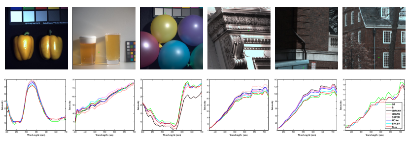
Figure 5: Visual comparison of the spectral signatures of pixels reconstructed by different methods. The positions of the corresponding pixels are marked by the green dot in RGB images. The spectral signatures by our PDE-Net are much closer to the ground-truth ones than the other compared methods, especially on the $1^{st}$ and $4^{th}$ columns.

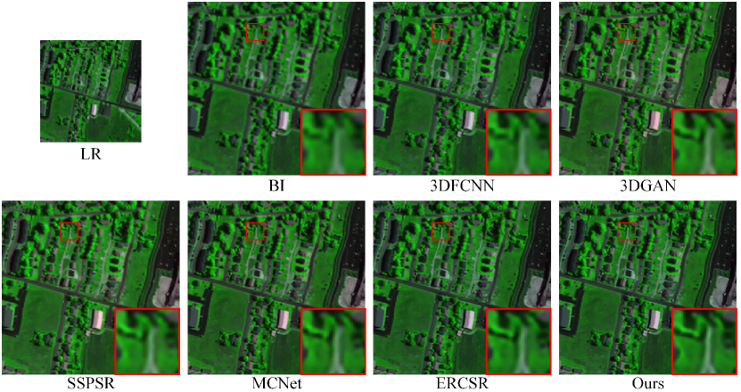
Figure 6: Visual comparison of different methods on the HS image from the Urban dataset ($\alpha=4$).

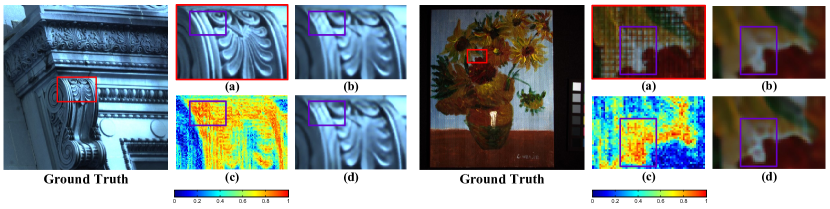
Figure 7: Visual illustration of the uncertainty estimation. (a) Zoomed-in patch in the red frame of the ground-truth HS images; (b) and (d) reconstructed HS images via two MC sampling; and (c): uncertainty maps. It could be observed that higher uncertainties correspond to larger variations of textures and higher risks of reconstruction errors.

We compared the proposed PDE-Net with 5 state-of-the-art deep learning-based methods, i.e., 3DFCNN [7], 3DGAN [8], SSPSR [11], MCNet [10], and ERCSR [9]. We also provided the results of bi-cubic interpolation (BI) as a baseline. For a fair comparison, we retrained all the compared methods with the same training data as ours by using the codes released by the authors with suggested settings. Besides, we applied the same data pre-processing to all methods.

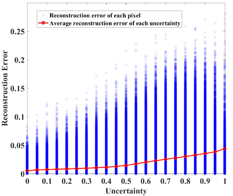
Figure 8: Visualization of the relationship between the uncertainty and reconstruction error of pixels. It can be observed that the average reconstruction error is approximately proportional to the pixel uncertainty.

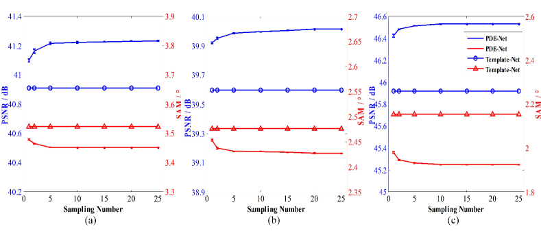
Figure 9: Illustration of the performance of our PDE-Net and Template-Net with different MC sampling times on three datasets ($\alpha=4$), i.e., (a) CAVE, (b) Harvard, and (c) NCALM.

Tables I, II, and III show the quantitative results of different methods on the three datasets, where it can be observed that

• our PDE-Net consistently achieves the best performance in terms of all the three metrics on all the three datasets when $\alpha=4$ and $8$, except the SAM value on the Harvard dataset for the $8\times$ super-resolution. Especially, our PDE-Net improves the MPSNR of the best existing methods by $0.53$ dB, $0.61$ dB, and $0.85$ dB (resp. $0.50$ dB, $0.12$ dB, and $0.29$ dB) over the CAVE, Harvard, and NCALM, respectively, when $\alpha=4$ (resp. 8). Moreover, the superiority of SSPSR [11] over our PDE-Net in terms of SAM under the $8\times$ super-resolution may benefit from the huge number of network parameters and the adopted spectral attention mechanism;

• the proposed Template-Net also obtains better reconstruction quality than most of the compared methods, demonstrating the superiority of our source-consistent HS images reconstruction framework to some extent;

• our PDE-Net further improves the Template-Net on the three datasets under all scenarios, validating the effectiveness and advantage of our posterior distribution-based HS embedding method; and

• for ERCSR [9] that always achieves the best or second-best performance among the compared methods, although it has a smaller number of network parameters than our PDE-Net, increasing its number of parameters cannot bring obvious performance improvement or even worsens performance [9], due to the network architecture limitation. Besides, as listed in Table V our PDE-Net with a comparable number of parameters to ERCSR still achieves better performance than ERCSR [9].

Besides, Fig. 4 visually compares the results by different methods, where we can observe that most high-frequency details are lost in the super-resolved images by the compared methods. By contrast, our PDE-Net produces results with sharper textures closer to the ground truth ones, which further demonstrates its advantage. In addition, Fig. 5 illustrates the spectral signatures of some pixels of reconstructed HR-HS images by different methods, where it can be seen that the shapes of the spectral signatures of all methods are generally consistent with those of the ground-truth ones. Moreover, the spectral signatures by our PDE-Net are closer to the ground-truth ones than the other methods, demonstrating the advantage of our method.

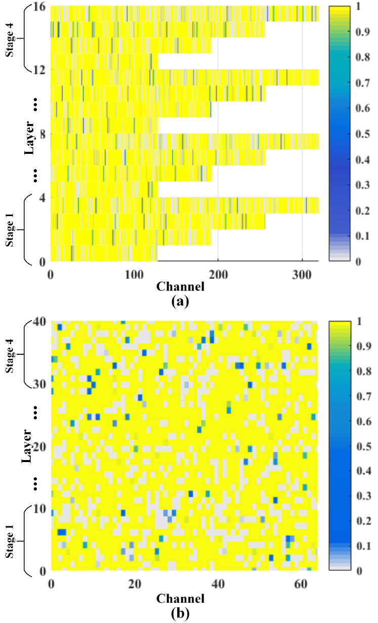
Figure 10: Visualization of network-level and layer-level probability space corresponding to the channels and layers of PDE-Net on the CAVE dataset for $4\times$ SR. (a) and (b) denote the network-level and layer-level distribution, respectively.

To demonstrate the robustness and generalization of our PDE-Net in practice, we also conducted the experiment in a real scenario, in which the input LR-HS is directly acquired by a typical sensor but not simulated by spatially downsampling the corresponding HR-HS image. Specifically, we utilized an HS image of spatial dimensions $307\times 307$ and spectral dimension 210 ranging from 400 to 2500 nm from the Urban dataset collected by the HYDICE hyperspectral system. Due to the limitation of computing resources, we only selected a region of size $128\times 128$ from the HS image for testing. Fig. 6 visually compares the results of different methods trained with the NCALM dataset, where it can be seen that the super-resolved image by our method shows clearer and sharper textures, demonstrating the advantage of our method. Note that the corresponding HR ground-truth HS image is not unknown, making it impossible to quantitatively compare different methods here.

Finally, we compared the computational efficiency of different methods measured with the inference time and the number of floating point of operations (#FLOPs) in Table IV. It can be seen that PDE-Net consumes less inference time and much fewer #FLOPs than most compared methods when performing MC sampling only once ($N=1$). Although #FLOPs grows linearly with the number of MC sampling (i.e., the value of $N$) increasing, we want to note that the MC-sampling process could be realized in a parallel manner as mentioned in Section III-D, and thus with more GPU nodes, the inference time of $N$ MC sampling could be comparable to that of 1 MC sampling. Besides, as illustrated in Fig. 9, the reconstruction quality increases relatively rapidly in the first 5 MC sampling but marginally when performing more MC sampling. Thus, in practice, one can perform MC sampling 5 times at most to save computational cost only with slight reconstruction quality sacrifice.

IV-C Ablation Study

IV-C1 The number of stages

To explore how the number of stages involved in our PDE-Net affects performance, we evaluated the PDE-Net with various numbers of stages, i.e., $T=2,~{}3,~{}4,~{}5,~{}6$ and $7$. From Table V, we can see that increasing the number of stages appropriately is able to improve the performance of both PDE-Net and Template-Net, demonstrating the rationality of the iterative refinement strategy on our source-consistent reconstruction framework. Especially, the PDE-Net is consistently better than Template-Net under all scenarios, which further indicates the effectiveness of our posterior distribution-based HS embedding method. Observing that when $T>4$, the performance of Template-Net is almost stable, and PDE-Net improves very slightly, we set the number of stages of our PDE-Net to 4 in all the remaining experiments of this paper.

IV-C2 The $\mathcal{L}_{2}$ loss

Table VI lists the reconstruction quality of our PDE-Net with and without the $\mathcal{L}_{2}$ loss during training, where it can be concluded that the $\mathcal{L}_{2}$ loss makes contributions to the reconstruction process of our PDE-Net. The reason is that employing $\mathcal{L}_{2}$ loss can not only regularize the reconstructed HR-HS image, but also guarantee the residual between the pseudo-LR-HS image and the input LR-HS image can be minimized progressively.

TABLE V: Results of the ablation study towards the number of stages ($T$) over the CAVE dataset ($\alpha=4$).

Stages	Methods	#Params	MPSNR$\uparrow$	MSSIM$\uparrow$	SAM$\downarrow$
2	Template-Net	1.147M	40.785	0.9663	3.556
	PDE-Net	1.151M	40.997	0.9668	3.477
3	Template-Net	1.721M	40.879	0.9667	3.520
	PDE-Net	1.726M	41.145	0.9671	3.457
4	Template-Net	2.295M	40.911	0.9666	3.514
	PDE-Net	2.301M	41.236	0.9672	3.455
5	Template-Net	2.868M	41.047	0.9666	3.509
	PDE-Net	2.877M	41.241	0.9672	3.437
6	Template-Net	3.442M	41.027	0.9664	3.497
	PDE-Net	3.452M	41.257	0.9670	3.439
7	Template-Net	4.016M	41.049	0.9667	3.495
	PDE-Net	4.028M	41.307	0.9674	3.434

TABLE VI: Results of the ablation study towards the $\mathcal{L}_{2}$ loss over the CAVE dataset ($\alpha=4$).

Methods	MPSNR$\uparrow$	MSSIM$\uparrow$	SAM$\downarrow$
PDE-Net w/o $\mathcal{L}_{2}$	41.083	0.9670	3.467
PDE-Net	41.236	0.9672	3.455

TABLE VII: Comparison of the proposed posterior distribution-based and NAS-based embedding schemes on the CAVE dataset ($\alpha=4$).

Methods	MPSNR$\uparrow$	MSSIM$\uparrow$	SAM$\downarrow$
NAS-based	41.085	0.9668	3.490
PDE-Net	41.236	0.9672	3.455

IV-C3 Illustration of the epistemic uncertainty

As shown in Figs. 7 and 8, as expected, the high uncertainty always occurs in the regions with highly-volatile textures and large reconstruction errors. Therefore, such epistemic uncertainty maps could help us to figure out the regions that are hard to handle, so that additional efforts or more advanced super-resolution techniques can be considered to improve these regions. Moreover, the predicted uncertainty may also give the confidence of network outputs in other HS image-based high-level applications, such as, HS image classification (assigning pixel-wise object categories to HS images) [59, 60] and object detection/tracking [61, 62][63, 64].

IV-C4 MC sampling

We validated how the MC sampling times affects the performance of our PDE-Net. Specifically, we calculated the mean value and standard deviation of MPSNRs/SAMs obtained via multiple MC sampling. As shown in Fig. 9, it can be observed that the PDE-Net consistently outperforms the Template-Net over all the three datasets. As the number of MC sampling gradually rising up, the average value of samples is gradually approaching the expectation of the distribution. Thus, the performance of PDE-Net gradually rises and finally achieves stable with the MC sampling times increasing.

IV-C5 Visualization of the learned posterior distribution

To have an intuitive understanding of our HS embedding architecture adaptively learned from the probabilistic perspective, we visualized the learned network-level and layer-level distributions in Fig. 10, where we can observe that the layer-level distribution is generally more complex than the network-level distribution, which is credited to the need of spatial-spectral diversities of local feature embedding.

IV-C6 Posterior Distribution-based vs. Network Architecture Search (NAS)-based embedding schemes

NAS-based schemes learn the network topology via maximum a posterior distribution [65], resulting in a determined network architecture. Although such an optimization scheme may produce the most possible model among the whole feasible set, compared to the proposed posterior distribution-based embedding, it discards a great number of plausible cases, which may also fit training samples well and contribute to performance improvement. To quantitatively compare these two embedding schemes, we constructed an NAS-based framework, in which with the same training data as ours and well-tuned hyperparameters, we trained our framework with the NAS strategy, to optimize the topology of the set of feasible HS embedding events $\mathcal{G}$. As shown in Table VII, our PDE-Net surpasses the NAS-based method in terms of all three metrics, demonstrating the advantage of our posterior distribution-based embedding scheme.

V Conclusion

We have proposed PDE-Net, a novel end-to-end learning-based framework for HS image super-resolution. We built PDE-Net on the basis of the intrinsic degradation relationship between LR and HR-HS images, thus making it physically-interpretable and compact. More importantly, we formulated HS embedding, a core module contained in the PDE-Net, from the probabilistic perspective to extract the high-dimensional spatial-spectral information efficiently and effectively. By conducting extensive experiments on three common datasets, we demonstrated the significant superiority of our PDE-Net over state-of-the-art methods both quantitatively and qualitatively. Besides, we provided comprehensive ablation studies to have a better understanding of the proposed PDE-Net.

Jinhui Hou received the B.E. and M.E. degrees in communication engineering from Huaqiao University, Xiamen, China, in 2017 and 2020, respectively. He is currently pursuing the Ph.D. degree in computer science with the City University of Hong Kong. His research interests include hyperspectral image processing and deep learning.

Zhiyu Zhu received the B.E. and M.E. degrees in Mechatronic Engineering, both from Harbin Institute of Technology, in 2017 and 2019, respectively. He is currently pursuing the Ph.D. degree in computer science with the City University of Hong Kong. His research interests include hyperspectral image processing and deep learning.

Junhui Hou (Senior Member, IEEE) is an Assistant Professor with the Department of Computer Science, City University of Hong Kong. He received the B.Eng. degree in information engineering (Talented Students Program) from the South China University of Technology, Guangzhou, China, in 2009, the M.Eng. degree in signal and information processing from Northwestern Polytechnical University, Xian, China, in 2012, and the Ph.D. degree in electrical and electronic engineering from the School of Electrical and Electronic Engineering, Nanyang Technological University, Singapore, in 2016. His research interests fall into the general areas of multimedia signal processing, such as image/video/3D geometry data representation, processing and analysis, graph-based clustering/classification, and data compression. He received the Chinese Government Award for Outstanding Students Study Abroad from China Scholarship Council in 2015 and the Early Career Award (3/381) from the Hong Kong Research Grants Council in 2018. He is an elected member of MSA-TC, VSPC-TC, and MMSP-TC. He is currently an Associate Editor for IEEE Transactions on Image Processing, IEEE Transactions on Circuits and Systems for Video Technology, Signal Processing: Image Communication, and The Visual Computer. He also served as the Guest Editor for the IEEE Journal of Selected Topics in Applied Earth Observations and Remote Sensing and as an Area Chair of ACM MM’19/20/21/22, IEEE ICME’20, VCIP’20/21/22, ICIP’22, and WACV’21.

Huanqiang Zeng (Senior Member, IEEE) received the B.S. and M.S. degrees in electrical engineering from Huaqiao University, China, and the Ph.D. degree in electrical engineering from Nanyang Technological University, Singapore. He is currently a Full Professor at the School of Engineering and the School of Information Science and Engineering, Huaqiao University. Before that, he was a Postdoctoral Fellow at The Chinese University of Hong Kong, Hong Kong. He has published more than 100 papers in well-known journals and conferences, including three best poster/paper awards (in the International Forum of Digital TV and Multimedia Communication 2018 and the Chinese Conference on Signal Processing 2017/2019). His research interests include image processing, video coding, machine learning, and computer vision. He has also been actively serving as the General Co-Chair for IEEE International Symposium on Intelligent Signal Processing and Communication Systems 2017 (ISPACS2017), the Co-Organizer for ICME2020 Workshop on 3D Point Cloud Processing, Analysis, Compression, and Communication, the Technical Program Co-Chair for Asia–Pacific Signal and Information Processing Association Annual Summit and Conference 2017 (APSIPA-ASC2017), the Area Chair for IEEE International Conference on Visual Communications and Image Processing (VCIP2015 and VCIP2020), and a technical program committee member for multiple flagship international conferences. He has been actively serving as an Associate Editor for IEEE Transactions on Image Processing, IEEE Transactions on Circuits and Systems for Video Technology, and Electronics Letters (IET). He has been actively serving as a Guest Editor for Journal of Visual Communication and Image Representation, Multimedia Tools and Applications, and Journal of Ambient Intelligence and Humanized Computing.

Jinjian Wu (Member, IEEE) received the B.Sc. and Ph.D. degrees from Xidian University, Xi’an, China, in 2008 and 2013, respectively. From 2011 to 2013, he was a Research Assistant with Nanyang Technological University, Singapore, where he was a Postdoctoral Research Fellow from 2013 to 2014. From 2015 to 2019, he was an Associate Professor with Xidian University, where he has been a Professor since 2019. His research interests include visual perceptual modeling, biomimetic imaging, quality evaluation, and object detection. He received the Best Student Paper Award/candidate at the ISCAS 2013/CICAI 2021. He has served as an Associate Editor for the journal of Circuits, Systems and Signal Processing (CSSP), the Special Section Chair for the IEEE Visual Communications and Image Processing (VCIP) 2017, and the Section Chair/Organizer/TPC Member for the ICME 2014-2015, PCM 2015-2016, VCIP 2018, AAAI 2019-2021, and ACM MM 2021-2022.

Jiantao Zhou (Senior Member, IEEE) received the B.Eng. degree from the Department of Electronic Engineering, Dalian University of Technology, in 2002, the M.Phil. degree from the Department of Radio Engineering, Southeast University, in 2005, and the Ph.D. degree from the Department of Electronic and Computer Engineering, Hong Kong University of Science and Technology, in 2009. He held various research positions with the University of Illinois at Urbana-Champaign, Hong Kong University of Science and Technology, and McMaster University. He is an Associate Professor with the Department of Computer and Information Science, Faculty of Science and Technology, University of Macau, and also the Interim Head of the newly established Centre for Artificial Intelligence and Robotics. His research interests include multimedia security and forensics, multimedia signal processing, artificial intelligence, and big data. He holds four granted U.S. patents and two granted Chinese patents. He has coauthored two papers that received the Best Paper Award at the IEEE Pacific-Rim Conference on Multimedia in 2007 and the Best Student Paper Award at the IEEE International Conference on Multimedia and Expo in 2016. He is serving as an Associate Editor for the IEEE TRANSACTIONS ON IMAGE PROCESSING and the IEEE TRANSACTIONS ON MULTIMEDIA.

References

- [1] B. Park and R. Lu, Hyperspectral imaging technology in food and agriculture. Springer, 2015.
- [2] B. Lu, P. D. Dao, J. Liu, Y. He, and J. Shang, “Recent advances of hyperspectral imaging technology and applications in agriculture,” Remote Sensing, vol. 12, no. 16, p. 2659, 2020.
- [3] M. Shimoni, R. Haelterman, and C. Perneel, “Hypersectral imaging for military and security applications: Combining myriad processing and sensing techniques,” IEEE Geoscience and Remote Sensing Magazine, vol. 7, no. 2, pp. 101–117, 2019.
- [4] J. Jia, Y. Wang, J. Chen, R. Guo, R. Shu, and J. Wang, “Status and application of advanced airborne hyperspectral imaging technology: A review,” Infrared Physics & Technology, vol. 104, p. 103115, 2020.
- [5] B. P. Banerjee, S. Raval, and P. Cullen, “Uav-hyperspectral imaging of spectrally complex environments,” International Journal of Remote Sensing, vol. 41, no. 11, pp. 4136–4159, 2020.
- [6] P. Mishra, M. S. M. Asaari, A. Herrero-Langreo, S. Lohumi, B. Diezma, and P. Scheunders, “Close range hyperspectral imaging of plants: A review,” Biosystems Engineering, vol. 164, pp. 49–67, 2017.
- [7] S. Mei, X. Yuan, J. Ji, Y. Zhang, S. Wan, and Q. Du, “Hyperspectral image spatial super-resolution via 3d full convolutional neural network,” Remote Sensing, vol. 9, no. 11, p. 1139, 2017.
- [8] J. Li, R. Cui, B. Li, R. Song, Y. Li, Y. Dai, and Q. Du, “Hyperspectral image super-resolution by band attention through adversarial learning,” IEEE Transactions on Geoscience and Remote Sensing, vol. 58, no. 6, pp. 4304–4318, 2020.
- [9] Q. Li, Q. Wang, and X. Li, “Exploring the relationship between 2d/3d convolution for hyperspectral image super-resolution,” IEEE Transactions on Geoscience and Remote Sensing, pp. 1–11, 2021.
- [10] Q. Li, Q. Wang, and X. Li, “Mixed 2d/3d convolutional network for hyperspectral image super-resolution,” Remote Sensing, vol. 12, no. 10, p. 1660, 2020.
- [11] J. Jiang, H. Sun, X. Liu, and J. Ma, “Learning spatial-spectral prior for super-resolution of hyperspectral imagery,” IEEE Transactions on Computational Imaging, vol. 6, pp. 1082–1096, 2020.
- [12] W. Dong, F. Fu, G. Shi, X. Cao, J. Wu, G. Li, and X. Li, “Hyperspectral image super-resolution via non-negative structured sparse representation,” IEEE Transactions on Image Processing, vol. 25, no. 5, pp. 2337–2352, 2016.
- [13] C. Yi, Y.-Q. Zhao, and J. C.-W. Chan, “Hyperspectral image super-resolution based on spatial and spectral correlation fusion,” IEEE Transactions on Geoscience and Remote Sensing, vol. 56, no. 7, pp. 4165–4177, 2018.
- [14] N. Akhtar, F. Shafait, and A. Mian, “Bayesian sparse representation for hyperspectral image super resolution,” in Proc. IEEE/CVF Conference on Computer Vision and Pattern Recognition, 2015, pp. 3631–3640.
- [15] Y. Xu, Z. Wu, J. Chanussot, and Z. Wei, “Nonlocal patch tensor sparse representation for hyperspectral image super-resolution,” IEEE Transactions on Image Processing, vol. 28, no. 6, pp. 3034–3047, 2019.
- [16] X. Han, B. Shi, and Y. Zheng, “Self-similarity constrained sparse representation for hyperspectral image super-resolution,” IEEE Transactions on Image Processing, vol. 27, no. 11, pp. 5625–5637, 2018.
- [17] R. Dian, L. Fang, and S. Li, “Hyperspectral image super-resolution via non-local sparse tensor factorization,” in Proc. IEEE/CVF Conference on Computer Vision and Pattern Recognition, 2017, pp. 3862–3871.
- [18] R. Dian, S. Li, and L. Fang, “Learning a low tensor-train rank representation for hyperspectral image super-resolution,” IEEE Transactions on Neural Networks and Learning Systems, vol. 30, no. 9, pp. 2672–2683, 2019.
- [19] R. Dian and S. Li, “Hyperspectral image super-resolution via subspace-based low tensor multi-rank regularization,” IEEE Transactions on Image Processing, vol. 28, no. 10, pp. 5135–5146, 2019.
- [20] J. Xue, Y.-Q. Zhao, Y. Bu, W. Liao, J. C.-W. Chan, and W. Philips, “Spatial-spectral structured sparse low-rank representation for hyperspectral image super-resolution,” IEEE Transactions on Image Processing, vol. 30, pp. 3084–3097, 2021.
- [21] M. R. Vicinanza, R. Restaino, G. Vivone, M. Dalla Mura, and J. Chanussot, “A pansharpening method based on the sparse representation of injected details,” IEEE Geoscience and Remote Sensing Letters, vol. 12, no. 1, pp. 180–184, 2014.
- [22] R. Fei, J. Zhang, J. Liu, F. Du, P. Chang, and J. Hu, “Convolutional sparse representation of injected details for pansharpening,” IEEE Geoscience and Remote Sensing Letters, vol. 16, no. 10, pp. 1595–1599, 2019.
- [23] Q. Xie, M. Zhou, Q. Zhao, D. Meng, W. Zuo, and Z. Xu, “Multispectral and hyperspectral image fusion by ms/hs fusion net,” in Proc. IEEE/CVF Conference on Computer Vision and Pattern Recognition, 2019, pp. 1585–1594.
- [24] J. Yao, D. Hong, J. Chanussot, D. Meng, X. Zhu, and Z. Xu, “Cross-attention in coupled unmixing nets for unsupervised hyperspectral super-resolution,” in Proc. European Conference on Computer Vision. Springer, 2020, pp. 208–224.
- [25] Y. Qu, H. Qi, and C. Kwan, “Unsupervised sparse dirichlet-net for hyperspectral image super-resolution,” in Proc. IEEE/CVF Conference on Computer vision and Pattern Recognition, 2018, pp. 2511–2520.
- [26] Z. Zhu, J. Hou, J. Chen, H. Zeng, and J. Zhou, “Hyperspectral image super-resolution via deep progressive zero-centric residual learning,” IEEE Transactions on Image Processing, vol. 30, pp. 1423–1438, 2021.
- [27] Z. Zhu, H. Liu, J. Hou, S. Jia, and Q. Zhang, “Deep amended gradient descent for efficient spectral reconstruction from single rgb images,” IEEE Transactions on Computational Imaging, vol. 7, pp. 1176–1188, 2021.
- [28] Z. Zhu, H. Liu, J. Hou, H. Zeng, and Q. Zhang, “Semantic-embedded unsupervised spectral reconstruction from single rgb images in the wild,” in Proceedings of the IEEE/CVF International Conference on Computer Vision, 2021, pp. 2279–2288.
- [29] S. Xie, C. Sun, J. Huang, Z. Tu, and K. Murphy, “Rethinking spatiotemporal feature learning: Speed-accuracy trade-offs in video classification,” in Proc. European Conference on Computer Vision, 2018, pp. 305–321.
- [30] Y. Wang, X. Chen, Z. Han, and S. He, “Hyperspectral image superresolution via nonlocal low-rank tensor approximation and total variation regularization,” Remote Sensing, vol. 9, no. 12, 2017.
- [31] H. Huang, J. Yu, and W. Sun, “Super-resolution mapping via multi-dictionary based sparse representation,” in Proc. IEEE International Conference on Acoustics, Speech and Signal Processing, 2014, pp. 3523–3527.
- [32] H. Zhang, L. Zhang, and H. Shen, “A super-resolution reconstruction algorithm for hyperspectral images,” Signal Processing, vol. 92, no. 9, pp. 2082–2096, 2012.
- [33] Y. Yuan, X. Zheng, and X. Lu, “Hyperspectral image superresolution by transfer learning,” IEEE Journal of Selected Topics in Applied Earth Observations and Remote Sensing, vol. 10, no. 5, pp. 1963–1974, 2017.
- [34] Y. Li, L. Zhang, C. Dingl, W. Wei, and Y. Zhang, “Single hyperspectral image super-resolution with grouped deep recursive residual network,” in Proc. IEEE Fourth International Conference on Multimedia Big Data, 2018, pp. 1–4.
- [35] J. Hu, X. Jia, Y. Li, G. He, and M. Zhao, “Hyperspectral image super-resolution via intrafusion network,” IEEE Transactions on Geoscience and Remote Sensing, vol. 58, no. 10, pp. 7459–7471, 2020.
- [36] N. Akhtar, F. Shafait, and A. Mian, “Hierarchical beta process with gaussian process prior for hyperspectral image super resolution,” in Proc. European Conference on Computer Vision, 2016, pp. 103–120.
- [37] C. Lanaras, E. Baltsavias, and K. Schindler, “Hyperspectral super-resolution by coupled spectral unmixing,” in Proc. IEEE/CVF International Conference on Computer Vision, 2015, pp. 3586–3594.
- [38] N. Akhtar, F. Shafait, and A. Mian, “Sparse spatio-spectral representation for hyperspectral image super-resolution,” in Proc. European Conference on Computer Vision, 2014, pp. 63–78.
- [39] W. Wang, W. Zeng, Y. Huang, X. Ding, and J. Paisley, “Deep blind hyperspectral image fusion,” in Proc. IEEE/CVF International Conference on Computer Vision, 2019, pp. 4149–4158.
- [40] L. Zhang, J. Nie, W. Wei, Y. Zhang, S. Liao, and L. Shao, “Unsupervised adaptation learning for hyperspectral imagery super-resolution,” in Proc. IEEE/CVF Conference on Computer Vision and Pattern Recognition, 2020, pp. 3070–3079.
- [41] Y. Qu, H. Qi, C. Kwan, N. Yokoya, and J. Chanussot, “Unsupervised and unregistered hyperspectral image super-resolution with mutual dirichlet-net,” IEEE Transactions on Geoscience and Remote Sensing, vol. 60, pp. 1–18, 2022.
- [42] Y. Romano and M. Elad, “Boosting of image denoising algorithms,” SIAM Journal on Imaging Sciences, vol. 8, no. 2, pp. 1187–1219, 2015.
- [43] X. Tao, C. Zhou, X. Shen, J. Wang, and J. Jia, “Zero-order reverse filtering,” in Proc. IEEE/CVF International Conference on Computer Vision, 2017, pp. 222–230.
- [44] W. Dong, H. Wang, F. Wu, G. Shi, and X. Li, “Deep spatial–spectral representation learning for hyperspectral image denoising,” IEEE Transactions on Computational Imaging, vol. 5, no. 4, pp. 635–648, 2019.
- [45] Q. Wang, Q. Li, and X. Li, “Spatial-spectral residual network for hyperspectral image super-resolution,” arXiv preprint arXiv:2001.04609, 2020.
- [46] Y. Gal and Z. Ghahramani, “Dropout as a bayesian approximation: Representing model uncertainty in deep learning,” in Proc. International Conference on Machine Learning, 2016, pp. 1050–1059.
- [47] E. Jang, S. Gu, and B. Poole, “Categorical reparameterization with gumbel-softmax,” in Proc. International Conference on Learning Representations (ICLR), 2016, pp. 1–12.
- [48] J. Kim, J. K. Lee, and K. M. Lee, “Accurate image super-resolution using very deep convolutional networks,” in Proc. IEEE/CVF Conference on Computer Vision and Pattern Recognition, 2016, pp. 1646–1654.
- [49] B. Lim, S. Son, H. Kim, S. Nah, and K. M. Lee, “Enhanced deep residual networks for single image super-resolution,” in Proc. IEEE/CVF Conference on Computer Vision and Pattern Recognition Workshops, 2017, pp. 1132–1140.
- [50] Y. Zhang, K. Li, K. Li, L. Wang, B. Zhong, and Y. Fu, “Image super-resolution using very deep residual channel attention networks,” in Proc. European Conference on Computer Vision, 2018, pp. 286–301.
- [51] T. Dai, J. Cai, Y. Zhang, S. Xia, and L. Zhang, “Second-order attention network for single image super-resolution,” in Proc. IEEE/CVF Conference on Computer Vision and Pattern Recognition, 2019, pp. 11 057–11 066.
- [52] F. Yasuma, T. Mitsunaga, D. Iso, and S. K. Nayar, “Generalized assorted pixel camera: Postcapture control of resolution, dynamic range, and spectrum,” IEEE Transactions on Image Processing, vol. 19, no. 9, pp. 2241–2253, 2010.
- [53] A. Chakrabarti and T. Zickler, “Statistics of real-world hyperspectral images,” in Proc. IEEE/CVF Conference on Computer Vision and Pattern Recognition, 2011, pp. 193–200.
- [54] Y. Xu, B. Du, L. Zhang, D. Cerra, M. Pato, E. Carmona, S. Prasad, N. Yokoya, R. Hänsch, and B. Le Saux, “Advanced multi-sensor optical remote sensing for urban land use and land cover classification: Outcome of the 2018 ieee grss data fusion contest,” IEEE Journal of Selected Topics in Applied Earth Observations and Remote Sensing, vol. 12, no. 6, pp. 1709–1724, 2019.
- [55] D. P. Kingma and J. Ba, “Adam: A method for stochastic optimization,” arXiv preprint arXiv:1412.6980, 2014.
- [56] Z. Wang and A. Bovik, “A universal image quality index,” IEEE Signal Processing Letters, vol. 9, no. 3, pp. 81–84, 2002.
- [57] R. H. Yuhas, A. F. Goetz, and J. W. Boardman, “Discrimination among semi-arid landscape endmembers using the spectral angle mapper (sam) algorithm,” in Proc. Summaries 3rd Annu. JPL Airborne Geosci. Workshop, vol. 1, 1992, pp. 147–149.
- [58] J. Jiang, D. Liu, J. Gu, and S. Süsstrunk, “What is the space of spectral sensitivity functions for digital color cameras?” in Proc. IEEE Workshop on Applications of Computer Vision. IEEE, 2013, pp. 168–179.
- [59] L. Mou, P. Ghamisi, and X. X. Zhu, “Deep recurrent neural networks for hyperspectral image classification,” IEEE Transactions on Geoscience and Remote Sensing, vol. 55, no. 7, pp. 3639–3655, 2017.
- [60] D. Hong, L. Gao, J. Yao, B. Zhang, A. Plaza, and J. Chanussot, “Graph convolutional networks for hyperspectral image classification,” IEEE Transactions on Geoscience and Remote Sensing, 2020.
- [61] J. Liang, J. Zhou, L. Tong, X. Bai, and B. Wang, “Material based salient object detection from hyperspectral images,” Pattern Recognition, vol. 76, pp. 476–490, 2018.
- [62] L. Zhang, Y. Zhang, H. Yan, Y. Gao, and W. Wei, “Salient object detection in hyperspectral imagery using multi-scale spectral-spatial gradient,” Neurocomputing, vol. 291, pp. 215–225, 2018.
- [63] B. Uzkent, A. Rangnekar, and M. Hoffman, “Aerial vehicle tracking by adaptive fusion of hyperspectral likelihood maps,” in Proc. IEEE/CVF Conference on Computer Vision and Pattern Recognition Workshops, 2017, pp. 39–48.
- [64] G. Tochon, J. Chanussot, M. Dalla Mura, and A. L. Bertozzi, “Object tracking by hierarchical decomposition of hyperspectral video sequences: Application to chemical gas plume tracking,” IEEE Transactions on Geoscience and Remote Sensing, vol. 55, no. 8, pp. 4567–4585, 2017.
- [65] H. Liu, K. Simonyan, and Y. Yang, “Darts: Differentiable architecture search,” in Proc. International Conference on Learning Representations (ICLR), 2019, pp. 1–13.