Direct and reverse precession of a massive vortex
in a binary Bose–Einstein condensate

Abstract

The dynamics of a filled massive vortex is studied numerically and analytically using a two-dimensional model of a two-component Bose–Einstein condensate trapped in a harmonic trap. This condensate exhibits phase separation. In the framework of the coupled Gross–Pitaevskii equations, it is demonstrated that, in a certain range of parameters of the nonlinear interaction, the precession of a sufficiently massive vortex around the center is strongly slowed down and even reverses its direction with a further increase in the mass. An approximate ordinary differential equation is derived that makes it possible to explain this behavior of the system.

Introduction

Ultracold gas mixtures consisting either of different chemical (alkaline) elements, or of different isotopes of the same element, or of the same isotopes in two different (hyperfine) quantum states exhibit a much wider variety of static and dynamic properties as compared to single-component Bose–Einstein condensates [1–5]. To a large extent, this is due to the presence of several parameters of nonlinear interactions, which are proportional to the corresponding scattering lengths and can sometimes be tuned over a wide range according to the aims of experimentalists using Feshbach resonances [6–10]. In particular, with a sufficiently strong mutual repulsion between two types of matter waves, a regime involving spatial separation of condensates is possible [11,12], in which domain walls are formed between the phases, characterized by effective surface tension [4,13]. Spatial separation can underlie many interesting configurations and phenomena, for example, the nontrivial geometry of the ground state of binary immiscible Bose–Einstein condensates in traps [14–16] (including optical lattices [17–19]), bubble dynamics [20], quantum analogs of classical hydrodynamic instabilities (Kelvin–Helmholtz [21,22], Rayleigh–Taylor [23–25], and Plateau–Rayleigh [26]), parametric instability of capillary waves at the interface [27,28], complex textures in rotating binary condensates [29–31], three-dimensional topological structures [32–37], capillary buoyancy of dense droplets in trapped immiscible Bose–Einstein condensates [38], etc.

In particular, vortices with a filled core in binary Bose–Einstein condensates and their dynamics are of considerable interest [3,39–45]. Such a structure can be represented as a quantized vortex in one of the components, the core of which is filled with the second component (see a numerical example in Fig.1). In this case, the dip in the density of the vortex component provides a potential well trapping the second (“bright”) component. In turn, the bright component creates a potential “hill that pushes” the vortex component apart and thereby increases the width of the vortex core. As a result, some equilibrium profile is formed in a self-consistent manner.

As compared to vortices in the $B$-phase of superfluid ³He occupied by the chiral $A$-phase, filled vortices in ultracold rarefied mixtures of Bose gases have a much simpler structure (for comparison, see review [46] and also [47]). In particular, in the core of a (stationary) cold gas vortex, the superfluid current has a simple structure ${\bf j}\propto[\rho_{1}(r)/r]{\bf e}_{\varphi}$ (in contrast to Fig.41 in [46], where there exists a counter-rotation region). Moreover, since binary Bose–Einstein condensates of cold atoms are described by a system of coupled Gross–Pitaevskii equations, in which the Hamiltonian contains no cross terms in the kinetic energy, there is no well-known Andreev–Bashkin effect, where the superfluid velocity of one component contributes to the current of another component [48, 49].

The vortex complex in the external potential of the trap, being deviated from the equilibrium position, begins to move nearly as a whole. One of the aims of researchers is the theoretical analysis of the emerging motion and the derivation of effective simplified equations for its description. For example, spatially two-dimensional models of binary condensates in a potential well with a flat bottom were recently considered in [42,43], where ordinary differential equations were proposed to determine the dynamics of massive “pointlike” vortices in such systems. At the same time, the practically important case of a smooth external potential remains unexplored. In this work, this gap is filled. Approximate equations of motion for massive vortices in smoothly inhomogeneous Bose–Einstein condensates are derived. These equations have a non-canonical Hamiltonian structure and, for one vortex, formally correspond to the dynamics of an electric charge in a certain static (two-dimensional) inhomogeneous electromagnetic field, where the electrostatic field lies in the $(x,y)$ plane, and the magnetic field is directed along the $z$ axis and is proportional to the equilibrium density $\rho(x,y)$ of the condensate without vortices.

(a)

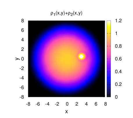
(b)

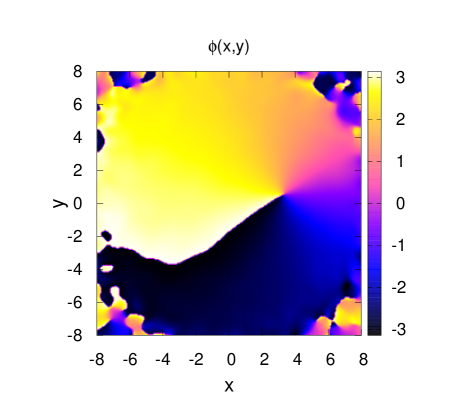
Figure 1: Numerical example of a filled vortex: (a) normalized total density of condensates and (b) the phase of the vortex component.

Analyzing the dependence of the parameters of this simplified model on the parameters of the original system of partial differential equations (in our case, these are coupled two-dimensional Gross–Pitaevskii equations), we reveal an interesting effect that has not yet been recognized for vortices in Bose–Einstein condensates. Namely, in the case of unequal nonlinear self-repulsion coefficients, the “electric” force in the case of a small filling of vortices with the bright component (having small effective mass) can be directed from the center of the system, and as the mass increases, it gradually decreases and then reverses its direction. This leads to a change in the direction of the vortex drift (its precession around the origin). We emphasize that, with such reverse precession, no qualitative rearrangement occurs inside the vortex core. Direct numerical simulations of the Gross–Pitaevskii equations will confirm the predictions of the simplified model.

Initial model

We consider a two-dimensional, sufficiently rarefied binary Bose–Einstein condensate in the limit of zero temperature, where the Gross–Pitaevskii equations are applicable. For maximum simplicity, it is assumed that both types of atoms have the same mass, $m_{1}=m_{2}=m$. Under this assumption, the case of a small difference in the masses of isotopes, such as ⁸⁵Rb and ⁸⁷Rb, can be described approximately. The harmonic trap is characterized by a transverse frequency $\omega$, which is the same for both types of atoms. We choose the scale $\tau=1/\omega$ for time, $l_{\rm tr}=\sqrt{\hbar/\omega m}$ for length, and $\varepsilon=\hbar\omega$ for energy. This allows us to write the equations of motion for the complex wavefunctions $A({\bf r},t)$ (vortex component) and $B({\bf r},t)$ (bright component) in the dimensionless form

$$i\dot{A}=-\frac{1}{2}\nabla^{2}A+\left[V(x,y)+g_{11}|A|^{2}+g_{12}|B|^{2}\right]A,$$ (1)

$$i\dot{B}=-\frac{1}{2}\nabla^{2}B+\left[V(x,y)+g_{21}|A|^{2}+g_{22}|B|^{2}\right]B,$$ (2)

where $V=(x^{2}+y^{2})/2$ is the trap potential and $g_{\alpha\beta}$ is the symmetric matrix of nonlinear interactions. The interactions can be physically described by the scattering lengths $a_{\alpha\beta}$ [2]:

$$g^{\rm phys}_{\alpha\beta}=2\pi\hbar^{2}a_{\alpha\beta}(m_{\alpha}^{-1}+m_{\beta}^{-1}).$$ (3)

Since we are interested in the situation where all scattering lengths are positive, the first self-repulsion factor can be normalized to unity, $g_{11}=1$. For only one component $A$ without any vortices, the equilibrium condensate density would be

$$|A_{0}|^{2}=\rho({\bf r})\approx[\mu-V(\bf r)],$$ (4)

where $\mu\gg 1$ is the chemical potential. The effective radius of the condensate is $R_{*}=\sqrt{2\mu}$. The motion of the massive vortex complex occurs against such inhomogeneous background.

The phase separation condition $g=(g^{2}_{12}-g_{11}g_{22})>0$ favors the existence of a filled vortex [11,12]. In a relatively narrow transient layer between the separated condensates, the densities of both phases nearly vanish in one or the opposite direction. However, for the applicability of the Gross–Pitaevskii equations, the width of this layer $\delta\sim 1/\sqrt{g\rho}$ should nevertheless be much larger than the characteristic scattering length $a$ (usually equal to several hundred Bohr radii), i.e., $\delta(l_{\rm tr}/a)\gg 1$. The corresponding energy excess (surface tension) is given by the expression

$$\sigma=K(g_{22}/g_{11},g_{12}/g_{11})\rho^{3/2},$$ (5)

where $K\sim\sqrt{g}$ at small $g$ [11,13]. Below, we will see that the dependence of the surface tension on the background density significantly affects the dynamics of a massive vortex, since it creates a gradient of its effective potential energy.

Structure of wavefunctions

When deriving the equations of vortex motion, we neglect the free excitations of acoustic vibrations and the deviation of the vortex shape from the circular one. The decisive factor allowing this to be done is the smallness of the ratio $w/R_{*}$, where $w$ is the radius of the vortex core and $R_{*}$ is the size of the condensate. Under this condition, the structure of the vortex is almost the same as that against the homogeneous background and its velocity is much lower than the velocities of potential excitations. As a result, the wavefunctions $A$ and $B$ can be approximately represented in the simplified form

$$A=\sqrt{\rho_{a}}e^{i\Phi_{a}}\approx\Psi_{v}({\bf r},{\bf R})\exp[i{\bf U}\cdot{\bf F}({\bf r},{\bf R})],$$ (6)

$$B=\sqrt{\rho_{b}}e^{i\Phi_{b}}\approx\Psi_{b}({\bf r},{\bf R})\exp[i{\bf U}\cdot{\bf G}({\bf r},{\bf R})],$$ (7)

where ${\bf R}(t)$ is the vortex position and ${\bf U}(t)$ is a certain two-dimensional vector, the relation of which to the vortex velocity will be revealed further on. It is very important that the function $\Psi_{v}$ involves a quantized vortex, and its phase $\Phi_{v}({\bf r})$ increases by $2\pi$ at the counterclockwise passing around the ${\bf R}$ point. The vortex phase $\Phi_{v}({\bf r})$ is appropriately matched to the density $\rho_{a}$, which coincides with $\rho({\bf r})$ far from the vortex, whereas $\rho_{a}\approx\varrho(|{\bf r}-{\bf R}|,{\bf R})$ inside its core, so that

$$\mbox{div}(\rho_{a}\nabla\Phi_{v})=0.$$ (8)

In turn, the densities $\varrho(|{\bf r}-{\bf R}|,{\bf R})$ and $\rho_{b}$ are matched to each other, as in the case of the filled vortex, against the locally homogeneous background density $\varrho(\infty,{\bf R})=\rho({\bf R})$. Additional functions ${\bf F}$ and ${\bf G}$ in the $A$ and $B$ phases are related to the parts of velocity fields that are due to the motion of the dip in the vortex component density and to the quasihomogeneous motion of the bright component, respectively. With a sufficient accuracy, we can assume that ${\bf G}={\bf r}-{\bf R}$ and ${\bf F}=({\bf r}-{\bf R})f(|{\bf r}-{\bf R}|,{\bf R})$, where the scalar function $f(\chi)$ at fixed ${\bf R}$ satisfies the second order linear differential equation

$$\varrho(\chi)[\chi f^{\prime\prime}+3f^{\prime}]+\varrho^{\prime}(\chi)[\chi f^{\prime}+f]=\varrho^{\prime}(\chi),$$ (9)

which follows from the continuity equation for the steady-state flow

$$\mbox{div}(\varrho[U_{i}F_{i,k}-U_{k}])=0.$$ (10)

Equation (9) is supplemented by the conditions that $f$ tends to zero at infinity and that the singularity at zero should be as weak as possible. It is very important that $f$ decreases rapidly at distances of the order of the vortex core width. The product ${\bf U}\cdot{\bf F}$ is qualitatively similar to the velocity potential that describes the flow around a cylinder in classical hydrodynamics and determines the corresponding added mass.

Simplified equations of motion for a vortex

We derive approximate equations of motion for the filled vortex based on the Hamiltonian structure of the Gross–Pitaevskii equations,

$$i\dot{A}=\delta{\cal H}/\delta A^{*},\qquad i\dot{B}=\delta{\cal H}/\delta B^{*},$$ (11)

where the Hamiltonian is given by the expression

$${\cal H} = \int\Big{[}\frac{|\nabla A|^{2}}{2}+\frac{|\nabla B|^{2}}{2}+V(x,y)(|A|^{2}+|B|^{2})$$ (12)

$$+\frac{g_{11}|A|^{4}}{2}+g_{12}|A|^{2}|B|^{2}+\frac{g_{22}|B|^{4}}{2}\Big{]}dxdy.$$

Using Eqs. (6), (7), and (11), we easily obtain the two relations

$$\int\Bigg{(}\dot{\rho}_{a}\frac{\partial\Phi_{a}}{\partial{\bf R}}-\dot{\Phi}_{a}\frac{\partial\rho_{a}}{\partial{\bf R}}\Bigg{)}dxdy+\{a\to b\}=\frac{\partial{\cal H}}{\partial{\bf R}},$$ (13)

$$\int\Bigg{(}\dot{\rho}_{a}\frac{\partial\Phi_{a}}{\partial{\bf U}}-\dot{\Phi}_{a}\frac{\partial\rho_{a}}{\partial{\bf U}}\Bigg{)}dxdy+\{a\to b\}=\frac{\partial{\cal H}}{\partial{\bf U}}.$$ (14)

Far from the vortex, either $\dot{\rho}_{a,b}$ or variational derivatives $\partial\rho_{a,b}/\partial{\bf R}$ are negligibly small (and $\partial\rho_{a,b}/\partial{\bf U}=0$ everywhere). Therefore, the main contribution to the integrals comes from the closest vicinity of the vortex, where we can use the approximate formulas

$$\dot{A} \approx -\dot{\bf R}\cdot\nabla A+iA(\dot{\bf U}\cdot{\bf F}),$$ (15)

$$\dot{B} \approx -\dot{\bf R}\cdot\nabla B+iB(\dot{\bf U}\cdot{\bf G}).$$ (16)

Substituting the time derivatives of densities and phases expressed from these formulas into Eqs. (13) and (14), we obtain after straightforward calculations two vector equations

$$-M\dot{\bf U}+2\pi[\hat{z}\times\dot{\bf R}]\rho({\bf R})\approx\partial H/\partial{\bf R},$$ (17)

$$M\dot{\bf R}\approx\partial H/\partial{\bf U},$$ (18)

where the scalar variable M is determined by the expression

$$M\delta_{ik}=\int(\rho_{a}F_{k,i}+\rho_{b}G_{k,i})dxdy.$$ (19)

It is clear that the Hamiltonian $H({\bf R},{\bf U})$ is quadratic in terms of ${\bf U}$ and should have the form

$$H\approx M_{tot}\frac{{\bf U}^{2}}{2}+W({\bf R}).$$ (20)

Therefore, one should identify ${\bf U}$ with the velocity of the vortex $\dot{\bf R}$, and then $M$ turns out to be the total effective mass of the filled vortex, which includes both the mass of the bright component $M_{br}$ trapped in the vortex core and the added mass of the vortex component due to the presence of additional kinetic energy during the motion of the density dip through the condensate.

In principle, the added mass $M_{add}$ could depend on ${\bf R}$; then, to preserve the conservative character of the system, we should introduce the vector ${\bf P}=M({\bf R}){\bf U}$ and rewrite the equations of motion in the “slightly corrected” form

$$-\dot{\bf P}+2\pi[\hat{z}\times\dot{\bf R}]\rho({\bf R})=\partial H/\partial{\bf R},$$ (21)

$$\dot{\bf R}=\partial H/\partial{\bf P}.$$ (22)

Probably, the generalization would be useful when considering strongly oblate three-dimensional condensates in the Thomas–Fermi regime along all three coordinates. However, it is easy to show that, in the case of strictly two-dimensional Gross–Pitaevskii equations, the mass $M_{add}$ in the leading approximation does not depend on the position of the vortex.

Estimates for the coefficients

If the effective radius $w$ of the vortex significantly exceeds the thickness of the domain wall $\delta$, then the added mass can be estimated using the well-known formula from classical hydrodynamics, i.e., $M_{add}\approx\pi\rho({\bf R})w^{2}$. On the other hand, since the hydrodynamic pressures of the condensates are $P_{a}=g_{11}\rho_{a}^{2}/2$ and $P_{b}=g_{22}\rho_{b}^{2}/2$, and they coincide in the leading order on both sides of the domain wall (if the surface tension $\sigma$ is not taken into account), the conservation of the mass of the bright component makes it possible to estimate the dependence $w({\bf R})$ using the condition

$$M_{br}=\pi\rho_{b}w^{2}=\pi\sqrt{\frac{g_{11}}{g_{22}}}\rho({\bf R})w^{2}=\sqrt{\frac{g_{11}}{g_{22}}}M_{add}.$$ (23)

In addition, this gives us also the estimate for the effective mass

$$M=[1+(g_{22}/g_{11})^{1/2}]M_{br}.$$ (24)

Since the total mass of a sufficiently large vortex turns out to be independent of its position on a spatially inhomogeneous background density, the derived system of equations (17) and (18) [taking into account Eq.(20)] is mathematically identical to the equation of the two-dimensional motion of an electric charge in magnetic and electric fields. The “electrostatic potential” $W({\bf R})$ in this case is equal to the sum of three contributions. The first contribution is the part of the kinetic energy that is due to the gradient of the vortex phase $\Phi_{v}({\bf r})$. The second contribution is the energy of nonlinear interactions plus the potential energy of the vortex in the field of the trap. The third contribution is the energy of “quantum pressure.” The first contribution in the well-known local induction approximation can be estimated as

$$W_{1}\approx\pi\Lambda_{0}\rho({\bf R}),\qquad\Lambda_{0}=\ln(R_{*}/w_{0}).$$ (25)

Note that $\Lambda_{0}\approx 2$ in practically interesting cases. The second and third contributions can be estimated (up to an insignificant additive constant) using the concept of surface tension,

$$W_{2}+W_{3}\approx 2\pi\sigma w+[1-(g_{22}/g_{11})^{1/2}]M_{br}U({\bf R})$$

$$=[\pi CM_{br}^{1/2}-[1-(g_{22}/g_{11})^{1/2}]M_{br}]\rho({\bf R}),$$ (26)

where $C$ is a coefficient about unity. Thus, the whole expression for the potential energy is reduced to the simple form

$$W({\bf R})=\pi\Lambda\rho({\bf R}),$$ (27)

where the effective dimensionless parameter $\Lambda$ depends in a nontrivial way on the mass of the trapped bright component,

$$\Lambda\approx\Lambda_{0}+CM_{br}^{1/2}-[1-(g_{22}/g_{11})^{1/2}]M_{br}/\pi.$$ (28)

Here, the second term is due to the surface tension at the phase boundary, and the third one is responsible for the “mass” contribution, taking into account the buoyant force. It is noteworthy that the hydrodynamic contribution $\Lambda_{0}$ can be significantly smaller than each of the other terms.

Vortex precession rate

In terms of the complex position $Z(t)=X(t)+iY(t)$, of the vortex, the resulting equation of motion for the massive vortex can be written as

$$-\tilde{M}\ddot{Z}+i(\mu-|Z|^{2}/2)\dot{Z}+\frac{\Lambda}{2}Z=0,$$ (29)

where $\tilde{M}=M/2\pi$. This equation is integrable in quadratures in an obvious way when passing to polar coordinates. We do not present the corresponding formulas here but note only that particular solutions in the form $Z(t)=R_{0}\exp(-i\Omega t)$ exist. The corresponding substitution gives two branches of the solution

$$\Omega_{\pm}(R_{0})=-\Big{[}\frac{(\mu-R_{0}^{2}/2)}{2\tilde{M}}\pm\sqrt{\frac{(\mu-R_{0}^{2}/2)^{2}-2\Lambda\tilde{M}}{4\tilde{M}^{2}}}\Big{]}.$$ (30)

Here, the solution $\Omega_{-}(R_{0})$, which corresponds to the charge drift in crossed magnetic and electric fields, is mainly of interest. It is seen that large positive values of $\Lambda$ promote a fast counterclockwise drift [negative frequency $\Omega_{-}(R_{0})$]. Moreover, both branches merge at some critical value of the radius, which decreases with increasing $\Lambda$. On the contrary, the drift is slowed down at small $\Lambda$ and reverses its direction (clockwise drift at positive frequency) at negative $\Lambda$. According to Eq.(28), the system under study has two features at $g_{22}\neq g_{11}=1$. First, the parameter $\Lambda$ at $g_{22}>1$ increases rapidly with the vortex mass, which should reduce the area of the stability of motion. Second, negative values of $\Lambda$ and reverse drift are possible at a sufficiently large vortex mass if $g_{22}<1$.

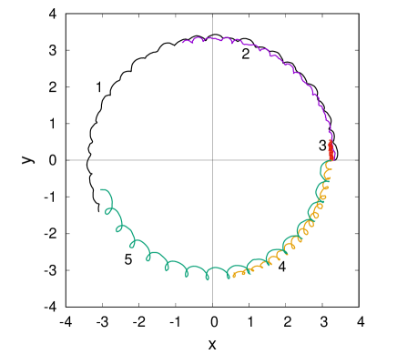
Figure 2: Examples of trajectories of a massive vortex in the time interval $[0:100]$ at $\mu=30$ for masses of the bright component $M_{br}/2\pi=$ (1) 8.0, (2) 10.0, (3) 12.0, (4) 14.0, and (5) 16.0. The motion begins at approximately the same point, but the direction and velocities of the drift are different.

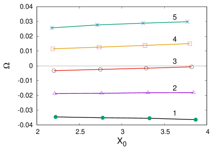
Figure 3: Numerically calculated drift angular velocity versus the initial coordinate at $g_{11}=g_{12}=1$, $g_{22}=0.5$, and $\mu=30$ for masses of the bright component $M_{br}/2\pi=$ (1) 8.0, (2) 10.0, (3) 12.0, (4) 14.0, and (5) 16.0.

Results of numerical tests

The parametric domain $\Lambda\gg 1$ will be studied elsewhere. Here, the prediction of the theory about the reverse drift is verified by direct numerical simulation of the coupled two-dimensional Gross–Pitaevskii equations. The performed calculations were focused on experimentally realized ⁸⁵Rb-⁸⁷Rb mixtures [8], where $a_{12}/a_{22}\approx 2$, while $a_{11}$ can be varied over a wide range using the Feshbach resonance. For this reason, in our numerical experiments, we took the values $g_{11}=g_{12}=1$, and $g_{22}=0.5$. The employed numerical method is similar to that used in [37,38,50].

The initial state for numerical integration was prepared in such a way that the filled vortex was located at some point ${\bf R}(0)=(X_{0},0)$ and had zero velocity. Next, its trajectory (the position of the center of mass of the bright component) was tracked and the drift angular velocity was calculated. Examples of the trajectories are shown in Fig.2. It is seen that fast oscillations characteristic of the charge motion in a magnetic field are superimposed on the slow drift. The plots of the drift angular velocity, confirming the possibility of the reverse motion, are shown in Fig.3.

Conclusions

To summarize, a simple equation of motion has been derived for a massive vortex in a two-dimensional smoothly inhomogeneous binary Bose–Einstein condensate and the possibility of reverse drift predicted by this equation has been numerically confirmed. The equation differs from a similar equation for a massless vortex in the natural additional term $M\ddot{\bf R}$ and in a different coefficient in the expression for the effective potential energy. There are even more possibilities for controlling the coefficients in the case of unequal atomic masses $m_{1}\neq m_{2}$ and at different external potentials $V_{1}({\bf r})\neq V_{2}({\bf r})$.

Note that a system of several massive vortices can be treated in a similar way. Technical difficulty appears only in the calculation of pair interactions. However, for some special equilibrium density profiles $\rho(x,y)$, this difficulty is successfully overcome, as shown in [51,52] for one-component Bose–Einstein condensates.

A strictly two-dimensional condensate is an idealization. A detailed test of the reverse precession regime for strongly oblate three-dimensional condensates is a task for the future. Preliminary numerical experiments have already shown a qualitative similarity to the planar case.

Conflict of interest

The author declares that he has no conflicts of interest.

References

- (1) Tin-Lun Ho and V. B. Shenoy, Phys. Rev. Lett. 77, 3276 (1996).
- (2) H. Pu and N. P. Bigelow, Phys. Rev. Lett. 80, 1130 (1998).
- (3) B. P. Anderson, P. C. Haljan, C. E. Wieman, and E. A. Cornell, Phys. Rev. Lett. 85, 2857 (2000).
- (4) S. Coen and M. Haelterman, Phys. Rev. Lett. 87, 140401 (2001).
- (5) G. Modugno, M. Modugno, F. Riboli, G. Roati, and M. Inguscio, Phys. Rev. Lett. 89, 190404 (2002).
- (6) J. P. Burke, Jr., J. L. Bohn, B. D. Esry, and C. H. Greene, Phys. Rev. Lett. 80, 2097 (1998).
- (7) G. Thalhammer, G. Barontini, L. De Sarlo, J. Catani, F. Minardi, and M. Inguscio, Phys. Rev. Lett. 100, 210402 (2008).
- (8) S. B. Papp, J. M. Pino, and C. E. Wieman, Phys. Rev. Lett. 101, 040402 (2008).
- (9) S. Tojo, Y. Taguchi, Y. Masuyama, T. Hayashi, H. Saito, and T. Hirano, Phys. Rev. A 82, 033609 (2010).
- (10) C. Chin, R. Grimm, P. Julienne, and E. Tiesinga, Rev. Mod. Phys. 82, 1225 (2010)
- (11) E. Timmermans, Phys. Rev. Lett. 81, 5718 (1998).
- (12) P. Ao and S. T. Chui, Phys. Rev. A 58, 4836 (1998).
- (13) B. Van Schaeybroeck, Phys. Rev. A 78, 023624 (2008).
- (14) A. A. Svidzinsky and S. T. Chui, Phys. Rev. A 68, 013612 (2003).
- (15) S. Gautam and D. Angom, J. Phys. B: At. Mol. Opt. Phys. 43, 095302 (2010).
- (16) R. W. Pattinson, T. P. Billam, S. A. Gardiner, D. J. McCarron, H. W. Cho, S. L. Cornish, N. G. Parker, and N. P. Proukakis, Phys. Rev. A 87, 013625 (2013).
- (17) K. Suthar, Arko Roy, and D. Angom, Phys. Rev. A 91, 043615 (2015).
- (18) K. Suthar and D. Angom, Phys. Rev. A 93, 063608 (2016).
- (19) K. Suthar and D. Angom, Phys. Rev. A 95, 043602 (2017).
- (20) K. Sasaki, N. Suzuki, and H. Saito, Phys. Rev. A 83, 033602 (2011).
- (21) H. Takeuchi, N. Suzuki, K. Kasamatsu, H. Saito, and M. Tsubota, Phys. Rev. B 81, 094517 (2010).
- (22) N. Suzuki, H. Takeuchi, K. Kasamatsu, M. Tsubota, and H. Saito, Phys. Rev. A 82, 063604 (2010).
- (23) K. Sasaki, N. Suzuki, D. Akamatsu, and H. Saito, Phys. Rev. A 80, 063611 (2009).
- (24) S. Gautam and D. Angom, Phys. Rev. A 81, 053616 (2010).
- (25) T. Kadokura, T. Aioi, K. Sasaki, T. Kishimoto, and H. Saito, Phys. Rev. A 85, 013602 (2012).
- (26) K. Sasaki, N. Suzuki, and H. Saito, Phys. Rev. A 83, 053606 (2011).
- (27) D. Kobyakov, V. Bychkov, E. Lundh, A. Bezett, and M. Marklund, Phys. Rev. A 86, 023614 (2012).
- (28) D. K. Maity, K. Mukherjee, S. I. Mistakidis, S. Das, P. G. Kevrekidis, S. Majumder, and P. Schmelcher, Phys. Rev. A 102, 033320, (2020).
- (29) K. Kasamatsu, M. Tsubota, and M. Ueda, Phys. Rev. Lett. 91, 150406 (2003).
- (30) K. Kasamatsu and M. Tsubota, Phys. Rev. A 79, 023606 (2009).
- (31) P. Mason and A. Aftalion, Phys. Rev. A 84, 033611 (2011).
- (32) K. Kasamatsu, M. Tsubota, and M. Ueda, Phys. Rev. Lett. 93, 250406 (2004).
- (33) H. Takeuchi, K. Kasamatsu, M. Tsubota, and M. Nitta, Phys. Rev. Lett. 109, 245301 (2012).
- (34) M. Nitta, K. Kasamatsu, M. Tsubota, and H. Takeuchi, Phys. Rev. A 85, 053639 (2012).
- (35) K. Kasamatsu, H. Takeuchi, M. Tsubota, and M. Nitta, Phys. Rev. A 88, 013620 (2013).
- (36) S. B. Gudnason and M. Nitta, Phys. Rev. D 98, 125002 (2018).
- (37) V. P. Ruban, J. Exp. Theor. Phys. 133, 779 (2021).
- (38) V. P. Ruban, JETP Lett. 113, 814 (2021).
- (39) K. J. H. Law, P. G. Kevrekidis, and L. S. Tuckerman, Phys. Rev. Lett. 105, 160405 (2010); Erratum, Phys. Rev. Lett. 106, 199903 (2011).
- (40) M. Pola, J. Stockhofe, P. Schmelcher, and P. G. Kevrekidis, Phys. Rev. A 86, 053601 (2012).
- (41) S. Hayashi, M. Tsubota, and H. Takeuchi, Phys. Rev. A 87, 063628 (2013).
- (42) A. Richaud, V. Penna, R. Mayol, and M. Guilleumas, Phys. Rev. A 101, 013630 (2020).
- (43) A. Richaud, V. Penna, and A. L. Fetter, Phys. Rev. A 103, 023311 (2021).
- (44) V. P. Ruban, JETP Lett. 113, 532 (2021).
- (45) V. P. Ruban, W. Wang, C. Ticknor, and P. G. Kevrekidis, Phys. Rev. A 105, 013319 (2022).
- (46) M. M. Salomaa and G. E. Volovik, Rev. Mod. Phys. 59, 533 (1987).
- (47) G. E. Volovik and T. Sh. Misirpashaev, JETP Lett. 51, 537 (1990).
- (48) A. F. Andreev and E. P. Bashkin, Sov. Phys. JETP 42, 164 (1976).
- (49) G. E. Volovik, JETP Lett. 115, 276 (2022).
- (50) V. P. Ruban, JETP Lett. 108, 605 (2018).
- (51) V. P. Ruban, J. Exp. Theor. Phys. 124, 932 (2017).
- (52) V. P. Ruban, JETP Lett. 105, 458 (2017).