Effect of Prefix/Suffix Configurations on OTFS Systems with Rectangular Waveforms

Abstract

Recently, orthogonal time-frequency-space (OTFS) modulation is used as a promising candidate waveform for high mobility communication scenarios. In practical transmission, OTFS with rectangular pulse shaping is implemented using different prefix/suffix configurations including reduced-cyclic prefix (RCP), full-CP (FCP), full-zero suffix (FZS), and reduced-zero padded (RZP). However, for each prefix/suffix type, different effective channel are seen at the receiver side resulting in dissimilar performance of the various OTFS configurations given a specific communication scenario. To fulfill this gap, in this paper, we study and model the effective channel in OTFS systems using various prefix/suffix configurations. Then, from the input-output relation analysis of the received signal, we show that the OTFS has a simple sparse structure for all prefix/suffix types, where the only difference is the phase term introduced when extending quasi-periodically in the delay-Doppler grid. We provide a comprehensive comparison between all OTFS types in terms of channel estimation/equalization complexity, symbol detection performance, power and spectral efficiencies, which helps in deciding the optimal prefix/suffix configuration for a specific scenario. Finally, we propose a novel OTFS structure namely reduced-FCP (RFCP) where the information of the CP block is decodable.

I Introduction

Having a reliable wireless communication link is always a challenge due the doubly-dispersive channel effect which introduces both ISI and ICI [1]. For instance, OFDM overcomes the high ISI causing frequency selectivity by dividing the whole transmission channel into smaller sub-channels in which fading is relatively considered flat [2]. This is achieved by the help of CP addition to the OFDM symbol which is longer than the delay spread of the channel. However, in time varying channels, OFDM performs poorly due the loss of orthogonality due to the Doppler shift, leading to ICI between the subcarriers [3, 4].

OTFS modulation has been recently introduced to parameterize the effect of the time-varying channels for any waveform by representing the channel in delay-Doppler domain where the real objects/reflectors in the propagation environment are seen, and thus, for a relatively short time frame the channel can be considered invariant [5]. The work in [5] was followed by various studies each addressing a distinct aspect of OTFS. For instance, [6] derived and investigated the high locality of delay-Doppler signals given a limited time and bandwidth using the Zak-transform. The effect of rectangular pulse shaping on the effective channel was studied in [7], where it was shown that using RCP with OFDM modulation ensures that the delay-Doppler channel is sparse. Channel estimation and equalization were discussed in [8], where a low complexity MMSE receiver is developed exploiting the sparse nature of the effective channel matrix in OTFS systems. Pilot design and detection were examined in [9], where a single pilot is embedded within the data frame protected by a two-dimensional (2D) guard in delay-Doppler domain. Then, at the receiver side after performing channel estimation, the data is detected using MP algorithm. OTFS-based MIMO systems are analyzed in [10], where the vectorized input-output relation is derived and accordingly a low complexity MP based iterative algorithm is presented for detection. The work in [11] investigated the performance of OTFS while exploiting the multi-user diversity in the downlink transmission. Finally, OTFS systems have been also studied under different hardware impairments such PAPR [12] and in-phase and quadrature imbalances [13].

However, the different ways of realizing OTFS systems are neither motivated nor differentiated one from another. For example, many research studies are based on the assumption of ideal waveform [8, 14] which is practically impossible due to Heisenberg’s uncertainty principle. Furthermore, some studies [15] neglect the phase term raised from the extension in delay-Doppler grid and assume that the data symbols in the delay-Doppler domain experience a constant channel gain, thus the effective channel matrix in delay-Doppler domain shows a doubly-circulant structure [16]. Also, when considering practical pulse shaping such as rectangular pulse shaping, many research works adopted different prefix/suffix structure. For instance, the authors in [12, 17] exploited the RCP configuration of OTFS, while the authors in [18] used FCP OTFS instead. In [19], the authors chose to use a ZS in order to combat the channel effects. However, except from the fact that the CP/ZS is appended to combat the channel dispersiveness, none of the studies mentioned above [6, 7, 8, 9, 10, 11, 12, 13, 15, 14, 20, 16, 17, 18, 19] have motivated the use of a certain type of prefix/suffix or their impact on the final result of the effective channel in delay-Doppler domain. Specifically, the prefix/suffix type determines whether the channel matrix is going to be block-diagonal, block-circulant, or neither. The structure of the channel matrix in turn dictates which signal processing techniques need to be utilized.

Taking into consideration the aforementioned problem, in this paper, the OTFS waveform is analyzed under different prefix/suffix configurations including RCP, RZP, FCP, and FZS, using rectangular pulse shaping. The conclusion of this analysis guides the researchers for the optimal OTFS design for a given scenario and system conditions. Thus, it would be easier to identify the most suitable OTFS structure based on the motivation of the study. The main contributions of this work are summarized as follows:

• We first derive the input-output relationship for the RCP, RZP, FCP, and FZS OTFS systems. It is shown that the received signal has a general structure regardless of the prefix/suffix configuration used in OTFS signal structure. The received signal’s structure varies in terms of the phase shift introduced when extending in the delay and Doppler grids. Also, it is deduced that in case of very low mobility or static channels, this phase term vanishes if FCP/FZS is used, where the convolution operation converts from 2D twisted convolution to a 2D circular one.

• We provide a comprehensive performance comparison between all OTFS types in terms of channel estimation/equalization complexity, symbol detection performance, power and spectral efficiencies. Given that the same detector is used, We show that the complexity and the detection performance are the same for all configurations.

• Then, the comparison between the full and the reduced prefix structure is made, and it is shown that the use of RCP OTFS is more advantageous, being more power and spectral efficient. Therefore, the use of FCP over RCP OTFS should be carefully selected due to the extra time and power resources needed in FCP implementation. For instance, FCP shows superiority over other types in a system with fractional Doppler channels.

• Finally, we propose a novel CP structure for OTFS signal namely reduced-FCP (RFCP) where RCP is appended to the FCP OTFS frame. Unlike the CP in OFDM signal, in the proposed RFCP OTFS, the CP block can be decodable instead of being discarded at the receiver side.

The rest of this paper is organized as follows; Section II presents the system model used for OTFS transmission. The effect of different prefix/suffix configurations is discussed in Section III. In Section IV, the results are analysed and discussed. Finally, Section V concludes the paper.

II System Model

II-A Transmitter

Consider a wireless communication system where $M\times N$ data symbols are modulated using OTFS transform. The OTFS modulator distributes these symbols $\{X_{\mathrm{DD}}(l,k),l=0,\dots,M-1~{},~{}k=0,\dots,N-1\}$ in the 2D delay-Doppler grid which is discretized into $M$ delays and $N$ Dopplers. Then, the samples $X_{\mathrm{DD}}(l,k)$ are converted to the time–frequency domain grid $\{X_{\mathrm{TF}}(n,m),~{}n=0,\dots,N-1,~{}m=0,\dots,M-1\}$ using the ISFFT as follows

$$X_{\mathrm{TF}}(n,m)=\frac{1}{\sqrt{MN}}\sum_{l=0}^{M-1}\sum_{k=0}^{N-1}X_{\mathrm{DD}}(l,k)e^{j2\pi\left(\frac{nk}{N}-\frac{ml}{M}\right)}.$$ (1)

To cast (1) from serial to matrix-vector form, we define $\mathbf{F}_{N}$ to be the $N\times N$ unitary DFT matrix; therefore, (1) is rewritten as

$$\mathbf{X}_{\mathrm{TF}}=\mathbf{F}_{M}\mathbf{X}_{\mathrm{DD}}\mathbf{F}_{N}^{H}.$$ (2)

Next, $\mathbf{X}_{\mathrm{TF}}$ is converted to time signal $\mathbf{s}$ by applying the Heisenberg transform. Then, $\mathbf{s}$ is transmitted over the doubly-dispersive channel as follows

$$\mathbf{s}=\operatorname{vec}\left(\mathbf{S}\right)=(\mathbf{F}_{N}^{H}\otimes\mathbf{I}_{M})\mathbf{x},$$ (3)

where $\mathbf{S}=\mathbf{X}_{\mathrm{DD}}\mathbf{F}_{N}^{H}$, $\mathbf{x}=\operatorname{vec}\left(\mathbf{X}_{\mathrm{DD}}\right)$, and $\mathbf{I}_{M}$ denotes the $M\times M$ identity matrix.

II-B Channel

Consider the $L$-tap doubly-selective CIR, modeling $L$ propagation paths in the environment as follows

$$h(\tau,\nu)=\sum_{i=0}^{L-1}h_{i}\delta(\tau-\tau_{i})\delta(\nu-\nu_{i}),$$ (4)

where $h_{i}$, $\tau_{i}=\frac{l_{i}}{M\Delta f}$ and $\nu_{i}=\frac{k_{i}}{NT}$ denote the complex channel gain, delay, and Doppler shift corresponding to the $i$-th path, respectively.

II-C Receiver

The received time-frequency signal $Y(n,m)$ is converted back to delay-Doppler domain via SFFT, as follows

$$y(l,k)=\sum_{n=0}^{N-1}\sum_{m=0}^{M-1}Y(n,m)e^{-j2\pi\left(\frac{nk}{N}-\frac{ml}{M}\right)}.$$ (5)

The input-output relation can be derived as

$$\mathbf{y} =\mathbf{H}_{\mathrm{eff}}\mathbf{x}+\mathbf{w}$$ (6)

$$=(\mathbf{F}_{N}\otimes\mathbf{I}_{M})\mathbf{H}(\mathbf{F}_{N}^{H}\otimes\mathbf{I}_{M})\mathbf{x}+\mathbf{w},$$

where $\mathbf{H}_{\mathrm{eff}}\in\mathbb{C}^{MN\times MN}$ and $\mathbf{H}\in\mathbb{C}^{MN\times MN}$ denote the delay-Doppler and the time equivalent channel matrices, respectively. Note that the channel matrices $\mathbf{H}$ and $\mathbf{H}_{\mathrm{eff}}$ cannot be written explicitly unless the type of prefix/suffix is determined. Accordingly, the following section will explain in detail the effect of different prefix/suffix types on the effective channel in time and delay-Doppler domains, and thus on the received signal.

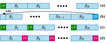
Figure 1: Different prefix/suffix configurations in OTFS systems: (a) RCP (b) RZP (c) FCP (d) FZS.

$$\mathbf{T}^{(i)}(kM+l,q)=\begin{cases}e^{-j2\pi\frac{k}{N}}z^{k_{i}\left(\left[l-l_{i}\right]_{M}\right)},&\text{ if }q=\left[l-l_{i}\right]_{M}+M\left[k-k_{i}\right]_{N}\text{ and }l<l_{i}\\ z^{k_{i}\left(\left[l-l_{i}\right]_{M}\right)},&\text{ if }q=\left[l-l_{i}\right]_{M}+M\left[k-k_{i}\right]_{N}\text{ and }l\geq l_{i}\\ 0,&\text{ otherwise }\end{cases}.$$ (17)

III Effect of Prefix/Suffix Configurations

In this section, the effect of using different types of prefix/suffix on the channel representation and received signal in OTFS systems is studied. Analysis starts by deriving effective channel expressions which will be used to develop the input-output relationship between the transmitted and received signals when using RCP (Fig. 1(a)), RZP (Fig. 1(b)), FCP (Fig. 1(c)), and FZS (Fig. 1(d)) configurations. Fractional Doppler shifts are not considered since the duration of one OTFS frame $NT$ is sufficient to capture the detailed channel information along the Doppler dimension over the typical wide-band systems. Hence, we assume that $l_{i}$ and $k_{i}$ are integer numbers. The case of both fractional delay and Doppler will be considered in our future work. After each derivation, a simple example will be demonstrated where a two-tap wireless doubly-dispersive channel with CIR $h(\tau,\nu)=h_{0}\delta(\tau-\frac{0}{M\Delta f})\delta(\nu-\frac{0}{NT})+h_{1}\delta(\tau-\frac{1}{M\Delta f})\delta(\nu-\frac{1}{NT})$ is assumed with $M=N=2$.

III-A Preliminaries

First, we introduce the lemma on the 2D-circular convolution.

Lemma1 : The circular convolution $C(m,n)=A(m,n)\circledast B(m,n)$ with $m=0,\dots,M-1,~{}n=0$ and $\dots,N-1$ can be expressed in a matrix form as

$$\mathbf{c}=\mathbf{A}\mathbf{b},$$ (7)

where $\mathbf{b}$ and $\mathbf{c}$ denote the vectorized form of $b(m,n)$ and $c(m,n)$, respectively. $\mathbf{A}$ is a doubly block circulant matrix generated from $a(m,n)$ with $N$ blocks, each of size $M\times M$, and it is given as

$$\mathbf{A}=\operatorname{Circ}\left(\mathbf{A}_{0},\dots,\mathbf{A}_{N-1}\right).$$ (8)

Each $\mathbf{A}_{n}$ is a $M\times M$ circulant matrix generated from the elements of the $n$-th row of $a(m,n)$, as follows

$$\mathbf{A}_{n}=\begin{pmatrix}a(n,0)&a(n,M-1)&\dots&a(n,1)\\ a(n,1)&a(n,0)&\dots&a(n,2)\\ \vdots&\vdots&\ddots&\vdots\\ a(n,M-1)&a(n,M-2)&\dots&a(n,0)\end{pmatrix}.$$ (9)

Theorem 1: The columns of the 2D ISFFT matrix i.e., $(\mathbf{F}_{N}^{-1}\otimes\mathbf{F}_{M})$ are eigenvectors of any doubly block circulant matrix $\mathbf{A}$. The corresponding eigenvalues are the 2D SFFT values of the 2D signal generating the doubly block circulant matrix as follows

$$\boldsymbol{\Sigma}=(\mathbf{F}_{N}\otimes\mathbf{F}_{M}^{-1})\mathbf{A}(\mathbf{F}_{N}^{-1}\otimes\mathbf{F}_{M}),$$ (10)

where $\boldsymbol{\Sigma}$ is a diagonal matrix containing the SFFT of $a(m,n)$ generating $\mathbf{A}$. Proof: Please refer to Appendix A. $\blacksquare$

Theorem 2: $\mathbf{A}$ can be block-diagonalized as follows [7]

$$\mathbf{A} =\left(\mathbf{F}_{N}^{-1}\otimes\mathbf{I}_{M}\right)\mathbf{D}\left(\mathbf{F}_{N}\otimes\mathbf{I}_{M}\right)$$ (11)

$$=\left(\mathbf{F}_{N}\otimes\mathbf{I}_{M}\right)\widetilde{\mathbf{D}}\left(\mathbf{F}_{N}^{-1}\otimes\mathbf{I}_{M}\right),$$

where $\mathbf{D}$ and $\widetilde{\mathbf{D}}$ are the block diagonal matrices given in [7].

III-B RCP

In RCP OTFS systems, only one CP is appended to the whole OTFS frame (see Fig. 1(a)); therefore, $\mathbf{H}^{\mathrm{R_{\mathrm{cp}}}}$ is expressed as

$$\mathbf{H}^{\mathrm{R_{\mathrm{cp}}}}=\sum_{i=0}^{L-1}h_{i}\boldsymbol{\Pi}^{l_{i}}_{MN}\boldsymbol{\Delta}^{k_{i}}_{MN},$$ (12)

with $\boldsymbol{\Pi}$ being the permutation matrix,

$$\boldsymbol{\Pi}_{MN}=\begin{pmatrix}0&\cdots&0&1\\ 1&\ddots&0&0\\ \vdots&\ddots&\ddots&\vdots\\ 0&\cdots&1&0\end{pmatrix}_{MN\times MN},$$ (13)

and $\boldsymbol{\Delta}_{MN}$ being the $MN\times MN$ diagonal matrix

$$\boldsymbol{\Delta}_{MN}^{k_{i}}=\operatorname{diag}\left[z_{i}^{0},z_{i}^{1},\ldots,z_{i}^{(MN-1)}\right],$$ (14)

with $z_{i}=e^{\frac{j2\pi k_{i}}{MN}}$. Then, the effective channel can be found as

$$\mathbf{H}_{\mathrm{eff}}^{\mathrm{R_{\mathrm{cp}}}}=(\mathbf{F}_{N}\otimes\mathbf{I}_{M})\mathbf{H}^{\mathrm{R_{\mathrm{cp}}}}(\mathbf{F}_{N}^{H}\otimes\mathbf{I}_{M}),$$ (15)

and it can also be expressed as [7]

$$\mathbf{H}_{\mathrm{eff}}^{\mathrm{R_{\mathrm{cp}}}}=\sum_{i=0}^{L-1}h_{i}\mathbf{T}^{(i)},$$ (16)

where $\mathbf{T}^{(i)}$ is given in (17). Note that $\mathbf{H}_{\mathrm{eff}}^{\mathrm{R_{\mathrm{cp}}}}$ has $L-1$ non-zero elements in each row and column, reflecting the sparsity nature of the effective delay-Doppler channel matrix. Then, the input-output relationship for each received sample $Y^{\mathrm{R_{\mathrm{cp}}}}(l,k)$ can be found as

$$Y^{\mathrm{R_{\mathrm{cp}}}}(l,k)=\sum_{i=0}^{L-1} h_{i}e^{j2\pi\frac{k_{i}}{N}\frac{l-l_{i}}{M}}\Lambda_{i}(l,k)$$ (18)

$$\times X_{\mathrm{DD}}\left(\left[l-l_{i}\right]_{M},\left[k-k_{i}\right]_{N}\right),$$

where

$$\Lambda_{i}(l,k)=\begin{cases}1&l_{i}\leq l<M\\ e^{-j2\pi\frac{k}{N}}&0\leq l<l_{i}\end{cases}.$$ (19)

Proof: Please refer to Appendix B. $\blacksquare$

Since $\mathbf{H}$ is not a block-diagonal matrix $\mathbf{H}_{\mathrm{eff}}$ will not be a block-circulant [7]. Hence, the relationship between the data and the delay-Doppler channel response is given by the 2-D twisted convolution [5], where a phase shift occurs as long we extend in the delay-Doppler axis. Consequently, the effective channel $\mathbf{H}_{\mathrm{eff}}$ will not be block circulant matrix. In line with our example, we find

$$\mathbf{H}^{\mathrm{R_{\mathrm{cp}}}}=\begin{pmatrix}h_{0}&0&0&{\color[rgb]{0,0,0}-jh_{1}}\\ h_{1}&h_{0}&0&0\\ 0&jh_{1}&h_{0}&0\\ 0&0&-h_{1}&h_{0}\end{pmatrix},$$ (20)

$$\mathbf{H}_{\mathrm{eff}}^{\mathrm{R_{\mathrm{cp}}}}=\begin{pmatrix}h_{0}&0&0&jh_{1}\\ 0&h_{0}&h_{1}&0\\ 0&-jh_{1}&h_{0}&0\\ h_{1}&0&0&h_{0}\end{pmatrix}.$$ (21)

As seen from (20), using one CP makes $\mathbf{H}^{\mathrm{R_{\mathrm{cp}}}}$ non-block diagonal which leads to a non-block circulant $\mathbf{H}_{\mathrm{eff}}^{\mathrm{R_{\mathrm{cp}}}}$ in (21) given that $\mathbf{H}_{\mathrm{eff}}^{\mathrm{R_{\mathrm{cp}}}}$ has non-zero elements equal to the number of channel taps in each row.

III-C RZP

In RZP OTFS systems, the whole OTFS frame is zero padded before transmission (see Fig. 1(b)). Then, at the receiver side the extra $L_{\mathrm{cp}}-1$ samples leaked from the received signal due to channel are extracted and added to the beginning of the OTFS frame. Consequently, due to the periodic nature of $\boldsymbol{\Delta}_{MN}^{k_{i}}$ the channel is equivalent to the one considered in RCP systems i.e., $\mathbf{H}_{\mathrm{eff}}^{\mathrm{R_{zp}}}=\mathbf{H}_{\mathrm{eff}}^{\mathrm{R_{\mathrm{cp}}}}$ thus $Y^{\mathrm{R_{zp}}}(l,k)=Y^{\mathrm{R_{cp}}}(l,k)$.

III-D FCP

In FCP OTFS systems, $N$ CPs of length $L_{\mathrm{cp}}\geq L$ are used to protect each OTFS subsymbol as in OFDM modulation (see Fig. 1(c)). Different from OFDM, where effective channel remains always the same as long as the CP duration is longer than the channel delay spread, OTFS’s effective channel matrix is a function of CP length in presence of Doppler. Particularly, the $(M+L_{\mathrm{cp}})N\times(M+L_{\mathrm{cp}})N$ channel matrix in this case can be given as

$$\hat{\mathbf{H}}^{\mathrm{F_{\mathrm{cp}}}}=\sum_{i=0}^{L-1}h_{i}\boldsymbol{\Pi}^{l_{i}}_{(M+L_{\mathrm{cp}})N}\boldsymbol{\Delta}^{k_{i}}_{(M+L_{\mathrm{cp}})N}.$$ (22)

Note that when using FCP the time duration of the OTFS frame increases, thus the Doppler resolution is higher compared to the case of RCP i.e., $z_{i}=e^{\frac{j2\pi k_{i}}{(M+L_{\mathrm{cp}})N}}\neq e^{\frac{j2\pi k_{i}}{MN}}$. This will be explained in Subsection IV-E.

After discarding the CPs, the channel matrix $\hat{\mathbf{H}}^{\mathrm{F_{\mathrm{cp}}}}$ becomes a block diagonal matrix with $N$ blocks, each of size $M\times M$ given as

$$\mathbf{H}^{\mathrm{F_{\mathrm{cp}}}}=\operatorname{diag}\left(\mathbf{H}_{0}^{\mathrm{F_{\mathrm{cp}}}},\dots,\mathbf{H}_{N-1}^{\mathrm{F_{\mathrm{cp}}}}\right),$$ (23)

where

$$\mathbf{H}_{n}^{\mathrm{F_{\mathrm{cp}}}}=\sum_{i=0}^{L-1}h_{i}\boldsymbol{\Pi}^{l_{i}}_{M}\boldsymbol{\Delta}^{k_{i},n}_{M},$$ (24)

and

$$\boldsymbol{\Delta}^{k_{i},n}_{M}=\operatorname{diag}\left[z_{i}^{n(M+L_{\mathrm{cp}})+L_{\mathrm{cp}}},\dots,z_{i}^{((n+1)(M+L_{\mathrm{cp}})-1)}\right].$$ (25)

From (25) we observe that the CP length will impact the estimated channel in the presence of Doppler. For different $L_{\mathrm{cp}}$ values, the resultant effective channel changes. The effective channel matrix can be expressed as

$$\mathbf{H}_{\mathrm{eff}}^{\mathrm{F_{\mathrm{cp}}}}=(\mathbf{F}_{N}\otimes\mathbf{I}_{M})\mathbf{H}^{\mathrm{F_{\mathrm{cp}}}}(\mathbf{F}_{N}^{H}\otimes\mathbf{I}_{M}).$$ (26)

Applying Theorem 2, we find

$$\mathbf{H}_{\mathrm{eff}}^{\mathrm{F_{\mathrm{cp}}}}=\operatorname{Circ}\left[\mathbf{G}^{\mathrm{F_{\mathrm{cp}}}}_{0},\ldots,\mathbf{G}^{\mathrm{F_{\mathrm{cp}}}}_{N-1}\right],$$ (27)

where

$$\mathbf{G}^{\mathrm{F_{\mathrm{cp}}}}_{n}=\sum_{\alpha=0}^{N-1}\mathbf{H}_{\alpha}^{\mathrm{F_{\mathrm{cp}}}}e^{-j2\pi n\alpha/N}.$$ (28)

Each element from $\mathbf{G}^{\mathrm{F_{\mathrm{cp}}}}_{n}$ can be computed as the DFT of the vector $\mathbf{g}_{\mathrm{cp}}^{(l^{\prime},k^{\prime})}$ conveying the $(l^{\prime},k^{\prime})$-th elements of $\mathbf{H}^{\mathrm{F_{\mathrm{cp}}}}_{n}$ i.e., $\mathbf{g}_{\mathrm{cp}}^{(l^{\prime},k^{\prime})}=[\mathbf{H}^{\mathrm{F_{\mathrm{cp}}}}_{0}(l^{\prime},k^{\prime}),\dots,\mathbf{H}^{\mathrm{F_{\mathrm{cp}}}}_{N-1}(l^{\prime},k^{\prime})]^{T}$ as follows

$$\mathbf{G}^{\mathrm{F_{\mathrm{cp}}}}_{n}(l^{\prime},k^{\prime}) =\mathbf{f}^{T}_{(n,N)}\cdot\mathbf{g}_{\mathrm{zs}}^{(l^{\prime},k^{\prime})}=\sum_{\alpha=0}^{N-1}\mathbf{H}_{\alpha}^{\mathrm{F_{\mathrm{cp}}}}(l^{\prime},k^{\prime})e^{-j2\pi n\alpha/N}$$ (29)

$$=\sum_{\alpha=0}^{N-1}\sum_{i=0}^{L-1}h_{i}z_{i}^{\left(\alpha(M+L_{\mathrm{cp}})+L_{\mathrm{cp}}+l^{\prime}-l_{i}\right)}e^{-j2\pi n\alpha/N}$$

$$~{}~{}~{}~{}~{}~{}~{}~{}~{}~{}~{}~{}~{}~{}\times\delta\left([l^{\prime}-k^{\prime}]_{M}-l_{i}\right),$$

where $\mathbf{f}_{(n,N)}$ denotes the $n$-th column of $\mathbf{F}_{N}^{H}$.

Proof: Please refer to Appendix C. $\blacksquare$

As seen from (29), $\mathbf{G}^{\mathrm{F_{\mathrm{cp}}}}_{n}$ is sparse and has at most one non-zero element in each row. Based on (6) and (26), the input-output relationship for each received sample $Y^{\mathrm{F_{\mathrm{cp}}}}(l,k)$ for the FCP structure can be derived as

$$Y^{\mathrm{F_{\mathrm{cp}}}}(l,k)=\sum_{i=0}^{L-1}h_{i}e^{\frac{j2\pi k_{i}(L_{\mathrm{cp}}+l-l_{i})}{(M+L_{\mathrm{cp}})N}}X_{\mathrm{DD}}\left(\left[l-l_{i}\right]_{M},\left[k-k_{i}\right]_{N}\right).$$ (30)

Proof: Please refer to Appendix D. $\blacksquare$

To have further insight, we again consider our example for the case when $L_{\mathrm{cp}}=2$. The corresponding effective channel matrices in time and delay-Doppler domains are respectively given as

$$\mathbf{H}^{\mathrm{F_{\mathrm{cp}}}}=\scalebox{1.0}{\mbox{$\displaystyle\begin{pmatrix}h_{0}&\frac{1+j}{2}h_{1}&0&0\\ jh_{1}&h_{0}&0&0\\ 0&0&h_{0}&-\frac{1+j}{2}h_{1}\\ 0&0&-jh_{1}&h_{0}\end{pmatrix}$}},$$ (31)

and

$$\mathbf{H}^{\mathrm{F_{\mathrm{cp}}}}_{\mathrm{eff}}=\scalebox{1.0}{\mbox{$\displaystyle\begin{pmatrix}h_{0}&0&0&\frac{1+j}{\sqrt{2}}h_{1}\\ 0&h_{0}&jh_{1}&0\\ 0&\frac{1+j}{\sqrt{2}}h_{1}&h_{0}&0\\ jh_{1}&0&0&h_{0}\end{pmatrix}$}},$$ (32)

As seen from (31), $\mathbf{H}^{\mathrm{F_{\mathrm{cp}}}}$ is block diagonal, thus $\mathbf{H}^{\mathrm{F_{\mathrm{cp}}}}_{\mathrm{eff}}$ is indeed block circulant with non-zero elements equal to the number of channel taps in each row as seen in (32).

Special case: If the channel is static (i.e., $k_{i}=0,~{}\forall i$), the input-output relation becomes 2D circular convolution between the data and the delay-Doppler CIR as follows

$$\scalebox{0.95}{\mbox{$\displaystyle Y^{\mathrm{F_{\mathrm{cp}}}}(l,k)=\sum_{i=0}^{L-1}h_{i}X_{\mathrm{DD}}\left(\left[l-l_{i}\right]_{M},\left[k-k_{i}\right]_{N}\right)=\mathbf{H}_{\mathrm{DD}}\circledast\mathbf{X}_{\mathrm{DD}}$}},$$ (33)

where $\mathbf{H}_{\mathrm{DD}}$ represents the delay-Doppler channel matrix. According to Lemma 1 and by using Theorem 1 the received signal in (33) can be expressed as

$$\mathbf{y}^{\mathrm{F_{\mathrm{cp}}}} =\mathbf{C}_{\mathrm{eff}}\mathbf{x}$$ (34)

$$=\left(\mathbf{F}_{N}^{-1}\otimes\mathbf{F}_{M}\right)\boldsymbol{\Sigma}\left(\mathbf{F}_{N}\otimes\mathbf{F}_{M}^{-1}\right)\mathbf{x},$$

where $\mathbf{C}_{\mathrm{eff}}$ is the doubly-circulant effective channel matrix. Since the channel can be simply equalized by element-wise division at the receiver side, the estimated symbols can be found as

$$\hat{\mathbf{x}}=\left(\mathbf{F}_{N}^{-1}\otimes\mathbf{F}_{M}\right)\boldsymbol{\Sigma}^{-1}\left(\mathbf{F}_{N}\otimes\mathbf{F}_{M}^{-1}\right)\mathbf{y}^{\mathrm{F_{\mathrm{cp}}}}.$$ (35)

III-E FZS

In the case of FZS OTFS, the last $L_{\mathrm{zs}}$ data symbols along the delay grid are set to zero. The FZS can also be seen as a zero-padded signal in the delay domain (see Fig. 1(d)). The transmitted signal can be shown as

$$X_{\mathrm{DD}}(l,k)=\begin{cases}d_{l,k},&\text{ if }l\leq M-L_{\mathrm{zs}}-1\\ 0,&\text{ if }l>M-L_{\mathrm{zs}}-1\end{cases},$$ (36)

where $d_{l,k}$ denotes the data symbols corresponding to $(l,k)$-th delay-Doppler index. The channel matrix of the FZS $\mathbf{H}^{\mathrm{F_{zs}}}$ can be represented in terms of $\mathbf{H}^{\mathrm{F_{\mathrm{cp}}}}$ as

$$\mathbf{H}^{\mathrm{F_{zs}}}=\operatorname{diag}\left(\mathbf{L}_{0}^{\mathrm{F_{\mathrm{zs}}}},\dots,\mathbf{L}_{N-1}^{\mathrm{F_{\mathrm{zs}}}}\right),$$ (37)

where $\mathbf{L}_{\alpha}^{\mathrm{F_{\mathrm{zs}}}}=\operatorname{TriL}(\mathbf{H}_{\alpha}^{\mathrm{F_{\mathrm{cp}}}})$. Using the fact that $\mathbf{H}^{\mathrm{F_{zs}}}$ is block-diagonal, we apply Theorem 2 to find the effective channel matrix as follows

$$\mathbf{H}_{\mathrm{eff}}^{\mathrm{F_{zs}}}=\operatorname{Circ}\left[\boldsymbol{\Omega}^{\mathrm{F_{zs}}}_{0},\ldots,\boldsymbol{\Omega}^{\mathrm{F_{zs}}}_{N-1}\right],$$ (38)

where

$$\boldsymbol{\Omega}^{\mathrm{F_{zs}}}_{n}=\sum_{\alpha=0}^{N-1}\mathbf{L}_{\alpha}^{\mathrm{F_{\mathrm{zs}}}}e^{-j2\pi n\alpha/N}.$$ (39)

Each element from $\boldsymbol{\Omega}^{\mathrm{F_{\mathrm{zs}}}}_{n}$ can be computed as the DFT of the vector $\mathbf{g}_{\mathrm{zs}}^{(l^{\prime},k^{\prime})}$ conveying the $(l^{\prime},k^{\prime})$-th elements of $\mathbf{L}^{\mathrm{F_{\mathrm{zs}}}}_{n}$ i.e., $\mathbf{g}_{\mathrm{zs}}^{(l^{\prime},k^{\prime})}=[\mathbf{L}^{\mathrm{F_{\mathrm{zs}}}}_{0}(l^{\prime},k^{\prime}),\dots,\mathbf{L}^{\mathrm{F_{\mathrm{zs}}}}_{N-1}(l^{\prime},k^{\prime})]^{T}$ as follows

$$\boldsymbol{\Omega}^{\mathrm{F_{zs}}}_{n}(l^{\prime},k^{\prime}) =\sum_{\alpha=0}^{N-1}\sum_{i=0}^{L-1}h_{i}z_{i}^{\alpha M+k^{\prime}}e^{-j2\pi nk/N}\cdot\delta\left(l^{\prime}-k^{\prime}-l_{i}\right).$$ (40)

Proof: Please refer to Appendix E. $\blacksquare$

The input-output relationship for the received sample $Y^{\mathrm{F_{zs}}}(l,k)$ for the FZS structure can be calculated as

$$Y^{\mathrm{F_{zs}}}(l,k)=\sum_{i=0}^{L-1}h_{i}e^{\frac{j2\pi k_{i}(l-l_{i})}{MN}}X_{\mathrm{DD}}\left(l-l_{i},\left[k-k_{i}\right]_{N}\right).$$ (41)

Proof: Please refer to Appendix F. $\blacksquare$

Following up with our example, we assume $L_{\mathrm{zs}}=1$. Then, the corresponding channel and effective channel matrices are respectively given as

$$\mathbf{H}^{\mathrm{F_{\mathrm{zs}}}}=\scalebox{1.0}{\mbox{$\displaystyle\begin{pmatrix}h_{0}&0&0&0\\ h_{1}&0&0&0\\ 0&0&h_{0}&0\\ 0&0&-h_{1}&0\end{pmatrix}$}},$$ (42)

and

$$\mathbf{H}^{\mathrm{F_{\mathrm{zs}}}}_{\mathrm{eff}}=\scalebox{1.0}{\mbox{$\displaystyle\begin{pmatrix}h_{0}&0&0&0\\ 0&0&h_{1}&0\\ 0&0&h_{0}&0\\ h_{1}&0&0&0\end{pmatrix}$}},$$ (43)

As seen from (42), $\mathbf{H}^{\mathrm{F_{\mathrm{zs}}}}$ is block diagonal with each block being lower triangular matrix, thus $\mathbf{H}^{\mathrm{F_{\mathrm{zs}}}}_{\mathrm{eff}}$ is indeed block circulant as seen in (43). Similar to the FCP case, when the channel is static, the input-output relation is also 2D circular convolution between the data and the delay-Doppler CIR.

IV Discussions And Results

In this section, we analyze and compare the different prefix/suffix OTFS waveforms based on the derivations obtained above. The comparison is made based on the received signal’s model, computational complexity of channel estimation/equalization, spectral and power efficiencies.

IV-A The Relation Between Different OTFS Configuration

From Section III, it is concluded that the received signal has a common form given as

$$Y(l,k)=\sum_{i=0}^{L-1}h_{i}\Gamma^{(i)}_{\eta}X_{\mathrm{DD}}\left[\left(l-l_{i}\right)_{M},\left(k-k_{i}\right)_{N}\right],$$ (44)

where $\Gamma^{(i)}_{\eta}(l,k,M,N,L_{\mathrm{cp/zs}})$ is a known phase term and ${\eta}$ denotes the type of prefix/suffix used $\eta=\{\text{RCP},\text{RZP},\text{FCP},\text{FZS}\}$. Therefore, finding the relation between the $\Gamma^{(i)}_{\eta}$ terms defines the correlation between the different OTFS realizations.

IV-A1 RCP & RZP

It is already shown in Subsection III-C that both RCP and RZP share the same received signal’s structure.

IV-A2 RCP & FCP

Consider a RCP OTFS system with $(M+L_{\mathrm{cp}})\times N$ data grid in delay-Doppler domain, then

$$\Gamma^{(i)}_{\text{RCP}}=e^{j2\pi\frac{k_{i}}{N}\frac{l-l_{i}}{(M+L_{\mathrm{cp}})}}\begin{cases}1&l_{i}\leq l<(M+L_{\mathrm{cp}})\\ e^{-j2\pi\frac{k}{N}}&0\leq l<l_{i}\end{cases}.$$ (45)

If the delays larger or equal to the CP length are selected (i.e., $\hat{l}=l+L_{\mathrm{cp}}\geq L_{\mathrm{cp}}$), the condition $l_{i}\leq\hat{l}<(M+L_{\mathrm{cp}})$ is satisfied. Therefore,

$$\Gamma^{(i)}_{\text{RCP}} (l+L_{\mathrm{cp}},k,M+L_{\mathrm{cp}},N)=e^{j2\pi\frac{k_{i}}{N}\frac{\hat{l}-l_{i}}{(M+L_{\mathrm{cp}})}}$$ (46)

$$=e^{j2\pi\frac{k_{i}}{N}\frac{L_{\mathrm{cp}}+l-l_{i}}{(M+L_{\mathrm{cp}})}}=\Gamma^{(i)}_{\text{FCP}}(l,k,M,N,L_{\mathrm{cp}}).$$

It is concluded that using FCP OTFS is equivalent to transmitting RCP OTFS with parameters $\hat{M}=M+L_{\mathrm{cp}}$ and $\hat{N}=N$, and considering only $M\times N$ symbols at the receiver side corresponding to indices $l=L_{\mathrm{cp}},\dots,M+L_{\mathrm{cp}}-1$ and $k=0,\dots,N-1$.

IV-A3 RCP & FZS

Consider a conventional RCP OTFS system with $M\times N$ data symbols in delay-Doppler domain; however, we set the last $(M-L_{\mathrm{zs}})\times N$ symbols to zero as follows

$$X_{\mathrm{DD}}(l,k)=\begin{cases}d_{l,k},&\text{ if }l\leq M-L_{\mathrm{zs}}-1\\ 0,&\text{ if }l>M-L_{\mathrm{zs}}-1\end{cases}.$$ (47)

If condition $0\leq l<l_{i}$ is true, then

$$\scalebox{0.95}{$X_{\mathrm{DD}}\left(\left[l-l_{i}\right]_{M},\left[k-k_{i}\right]_{N}\right)=X_{\mathrm{DD}}\left(l-l_{i}+M,\left[k-k_{i}\right]_{N}\right)=0$}.$$ (48)

This means that for $~{}0\leq l<l_{i}$, $\Gamma^{(i)}(l,k)$ can take any value since it is multiplied by zero according to (48). Then, we can generalize the phase term to be

$$\Gamma^{(i)}_{\text{RCP}}(l,k,M,N,\eqref{equ:cond}) =e^{j2\pi\frac{k_{i}}{N}\frac{l-l_{i}}{M}},~{}~{}~{}\forall l$$ (49)

$$=\Gamma^{(i)}_{\text{FZS}}(l,k,M,N,L_{\mathrm{zs}}).$$

Therefore, we conclude that using FZS OTFS is equivalent to transmitting RCP OTFS with parameters $M$ and $N$, and setting symbols corresponding to indices $l=M-L_{\mathrm{zs}},\dots,M-1$ and $k=0,\dots,N-1$ to zero.

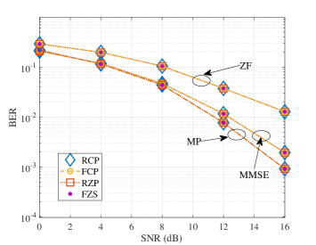
Figure 2: Performance comparison of MP, ZF, and MMSE detectors based OTFS with different prefix/suffix types using $(M;N;L_{\mathrm{cp}},L_{\mathrm{zs}})=(16,16,4,4)$. The number of paths in the delay-Doppler domain is $L=4$.

IV-B Channel Estimation

From Subsection IV-A, we found out that regardless of the prefix/suffix type, the received signal has a common formula expressed by (44). Therefore, we can conclude that the computational complexity and the performance of a specific channel estimation/equalization algorithm and detection method are the same no matter what prefix/suffix configuration is used in OTFS systems. Three detectors are considered in the simulations, namely, the MP detector proposed in [21], ZF receiver [22] expressed by

$$\mathbf{x}_{\mathrm{ZF}}=\mathbf{H}_{\mathrm{eff}}^{H}\left(\mathbf{H}_{\mathrm{eff}}\mathbf{H}_{\mathrm{eff}}^{H}\right)^{-1},$$ (50)

and the classic MMSE detector given by [8]

$$\mathbf{x}_{\mathrm{MMSE}}=\mathbf{H}_{\mathrm{eff}}^{H}\left(\mathbf{H}_{\mathrm{eff}}\mathbf{H}_{\mathrm{eff}}^{H}+\sigma^{2}\mathbf{I}\right)^{-1},$$ (51)

where $\sigma^{2}$ denotes the AWGN noise variance. The results are depicted in Fig. 2, where it is seen that the average BER performances of RCP, RZP, FCP, and FSZ are almost identical when MP, ZF, or MMSE detectors are implemented for symbol detection. MMSE detector performs better than ZF since it exploits noise statistics in detection, whereas MP outperforms both because it exploits the noise statistics as well as the diversity from different channel taps.

IV-C Spectral & Power Efficiencies

The total spectral and power efficiencies in OTFS systems depend directly on the prefix/suffix configuration used. To show that, consider the capacity $C$ for a given instantaneous SNR $\gamma$ as follows [23]

$$C_{R_{\mathrm{cp}}}=\left(\frac{MN}{MN+L_{\mathrm{cp}}}\right)\log_{2}\left(1+\gamma\right)$$ (52a)

$$C_{R_{\mathrm{zp}}}=\left(\frac{MN}{MN+L_{\mathrm{cp}}}\right)\log_{2}\left(1+\gamma\right)$$ (52b)

$$C_{F_{\mathrm{cp}}}=\left(\frac{M}{M+L_{\mathrm{cp}}}\right)\log_{2}\left(1+\gamma\right)$$ (52c)

$$C_{F_{\mathrm{zs}}}=\left(\frac{M-L_{\mathrm{zs}}}{M}\right)\log_{2}\left(1+\gamma\right).$$ (52d)

Regarding the power efficiency, the average transmitted power is considered as follows [24]

$$P=E\left\{\int_{0}^{T^{\prime}}|s(t)|^{2}dt\right\}=\int_{0}^{T^{\prime}}E\left\{|s(t)|^{2}\right\}dt,$$ (53)

where $T^{\prime}$ is the transmitted frame’s length and $E\left\{|s(t)|^{2}\right\}$ is the average symbol power. Therefore, under the constraint that all OTFS configurations have the same capacity, the average transmitted powers for each OTFS configuration are given as

$$P_{R_{\mathrm{cp}}}=\left(MN+L_{\mathrm{cp}}\right)E\left\{|s(t)|^{2}\right\}$$ (54a)

$$P_{R_{\mathrm{zp}}}=\left(MN\right)E\left\{|s(t)|^{2}\right\}$$ (54b)

$$P_{F_{\mathrm{cp}}}=N\left(M+L_{\mathrm{cp}}\right)E\left\{|s(t)|^{2}\right\}$$ (54c)

$$P_{F_{\mathrm{zs}}}=\left(MN\right)E\left\{|s(t)|^{2}\right\}.$$ (54d)

As seen from (52) and (54), RZP OTFS achieves the best attainable performance in terms of both metrics, where RCP OTFS losses some power efficiency due to its CP but this would provide better synchronization performance and smoother transition between the OTFS frames. The last two types namely, FZS and FCP OTFS have the worst power and spectral efficiencies, respectively. Fig. 3 and Fig. 4 emphasizes the above results. For instance, Fig. 3 shows that RCP and RZP provide the highest capacities which are almost invariant for the cases of $L_{\mathrm{cp}}=8$ and $L_{\mathrm{cp}}=16$. In fact, the zoomed part of Fig. 3 illustrates that there is a performance different when $L_{\mathrm{cp}}$ changes, however, for sufficiently large $MN$ the capacities $C_{R_{\mathrm{cp}}}$ and $C_{R_{\mathrm{zp}}}$ can be approximated to

$$C_{R_{\mathrm{cp}}}=C_{R_{\mathrm{zp}}}\approx\log_{2}\left(1+\gamma\right);~{}~{}~{}~{}MN\gg\ 1.$$ (55)

Whereas the capacities of FCP and FZS improve as the CP length value decreases. Fig. 4 shows the transmitted power needed to achieve a specific capacity assuming that $E\left\{|s(t)|^{2}\right\}=1$. For $N=32$ the transmitted power for RCP, RZP, and FZS is shown to be not effect by $L_{\mathrm{cp}}$, unlike FCP scheme that transmits higher power than all other prefix/suffix schemes. This power is proportional to $L_{\mathrm{cp}}$. As the subcarrier number $M$ increases, the transmitted power of all configurations converges to $P=\left(MN\right)E\left\{|s(t)|^{2}\right\}$.

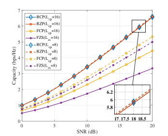
Figure 3: OTFS system’s capacity using different prefix/suffix configurations with $(M;N)=(32,32)$.

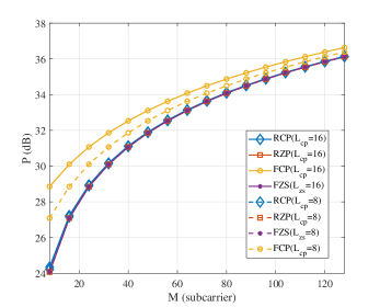
Figure 4: The transmitted power required in OTFS system versus the total number of subcarriers $M$ for a given capacity and a fixed $N=32$.

IV-D Fractional Doppler

TABLE I: Comparison between the different prefix/suffix OTFS configuration.

	RCP	RZP	FCP	FZS
Phase Term $\Gamma^{(i)}$	$e^{j2\pi\frac{k_{i}}{N}\frac{l-l_{i}}{M}}\begin{cases}1&l_{i}\leq l<M\\ e^{-\frac{j2\pi k}{N}}&0\leq l<l_{i}\end{cases}$	$e^{j2\pi\frac{k_{i}}{N}\frac{l-l_{i}}{M}}\begin{cases}1&l_{i}\leq l<M\\ e^{-\frac{j2\pi k}{N}}&0\leq l<l_{i}\end{cases}$	$e^{\frac{j2\pi k_{i}(L_{\mathrm{cp}}+l-l_{i})}{(M+L_{\mathrm{cp}})N}}$	$e^{j2\pi\frac{k_{i}}{N}\frac{l-l_{i}}{M}}$
$\Gamma^{(i)}$ in Static Channel	$\begin{cases}1&l_{i}\leq l<M\\ e^{-j2\pi\frac{k}{N}}&0\leq l<l_{i}\end{cases}$	$\begin{cases}1&l_{i}\leq l<M\\ e^{-j2\pi\frac{k}{N}}&0\leq l<l_{i}\end{cases}$	$1$	$1$
Power Efficiency $E\left\{|s(t)|^{2}\right\}=1$	$\frac{1}{MN+L_{\mathrm{cp}}}$	$\frac{1}{MN}$	$\frac{1}{N(M+L_{\mathrm{cp}})}$	$\frac{1}{MN}$
Spectral Efficiency	$\frac{MN}{MN+L_{\mathrm{cp}}}$	$\frac{MN}{MN+L_{\mathrm{cp}}}$	$\frac{M}{M+L_{\mathrm{cp}}}$	$\frac{M-L_{\mathrm{cp}}}{M}$

One advantage of using full prefix rather than reduced prefix/suffix can be extracted from (30), where we see that the Doppler resolution is a function of the CP length $L_{\mathrm{cp}}$. Thus, not only FCP has higher Doppler resolution compared to RCP/ZP OTFS but also the Doppler resolution itself is adaptive and can be controlled by changing the $L_{\mathrm{cp}}$ to achieve less inter-Doppler interference in the system.

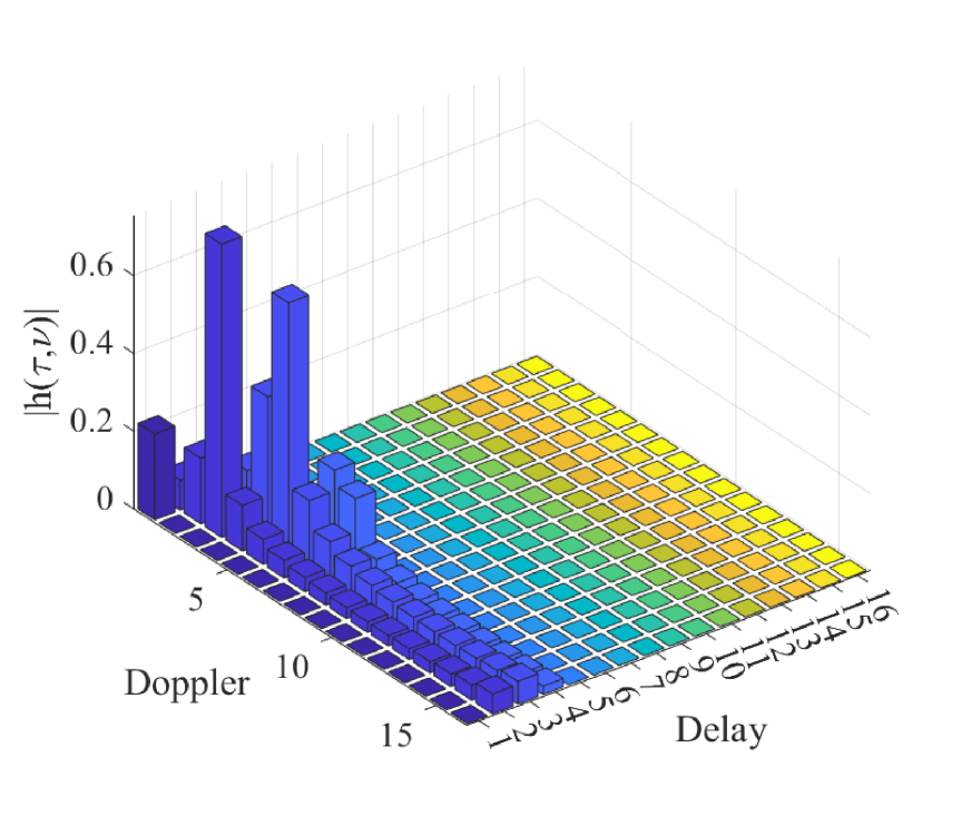
(a) $L_{\mathrm{cp}}=4$.

(b) $L_{\mathrm{cp}}=6$.

Figure 5: The delay-Doppler CIR of FCP OTFS under fractional Doppler using different CP lengths. The number of paths in the delay-Doppler domain is $L=4$.

Fig. 5 depicts the delay-Doppler CIR in the existence of fractional Doppler. it is observed that as $L_{\mathrm{cp}}$ changes, the channel profile changes as well. For instance, when $L_{\mathrm{cp}}=4$ the channel suffers from high inter-Doppler interference which vanishes at $L_{\mathrm{cp}}=6$. Fig. 6 shows that fractional Doppler kills the BER performance of RCP, RZP, and FZS. However, in case of FCP, the BER performance changes as the CP length changes and achieves the best performance at $L_{\mathrm{cp}}=6$ emphasizing the results depicted in Fig. 5. Table I summarizes the main differences between different OTFS implementations.

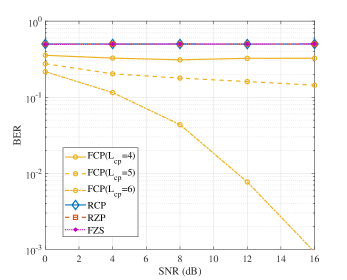
Figure 6: The BER performance vs SNR of OTFS under fractional Doppler using different OTFS configurations and different CP lengths. The number of paths in the delay-Doppler domain is $L=4$.

IV-E Reduced or Full?

The full prefix/suffix is different from the reduced one in terms of interpretation even though they mainly share the same task of combating channel effects. RCP OTFS can resemble to CP-OFDM, where the CP is appended to the beginning of the frame; however, most importantly this CP has no meaning on its own since it is generated from the combination of the whole data symbols, which is the reason why it is discarded the receiver side [25]. On the other hand, the CP in FCP OTFS is interpretable and conveys data which can be extracted and decoded. Consider $\mathbf{P}^{\mathrm{F_{\mathrm{cp}}}}\in\mathbb{C}^{(M+L_{\mathrm{cp}})\times M}$ the CP addition matrix [26], the 2D transmit signal can be given as follows

$$\mathbf{S}^{\mathrm{F_{\mathrm{cp}}}} =\mathbf{P}^{\mathrm{F_{\mathrm{cp}}}}\mathbf{S}=\mathbf{P}^{\mathrm{F_{\mathrm{cp}}}}\mathbf{X}_{\mathrm{DD}}\mathbf{F}_{N}^{H}$$ (56)

$$=\mathbf{X}_{\mathrm{DD}}^{\mathrm{F_{\mathrm{cp}}}}\mathbf{F}_{N}^{H},$$

where $\mathbf{X}_{\mathrm{DD}}^{\mathrm{F_{\mathrm{cp}}}}=\mathbf{P}^{\mathrm{F_{\mathrm{cp}}}}\mathbf{X}_{\mathrm{DD}}$ represents the extended OTFS frame in the delay-Doppler domain. Therefore, adding FCP is equivalent to extending the delay-Doppler grid to $(M+L_{\mathrm{cp}})\times N$ by repeating the last $L_{\mathrm{cp}}$ rows of $\mathbf{X}_{\mathrm{DD}}$. Also, this explains why the Doppler resolution in (22) is $(M+L_{\mathrm{cp}})\times N$ instead of $M\times N$ as in RCP OTFS. Fig. 7 graphically illustrates the relationship between adding the CP in delay-Doppler and time domains in FCP OTFS system. So, spending more valuable resources to transmit repeated data, which could be replaced with unknown data symbols seems futile, knowing that one CP is enough to protect the whole OTFS frame and that the computational complexity and the performance of channel estimation/equalization and data detection are the same.

Therefore, we conclude that the use of FCP OTFS should be well motivated otherwise RCP OTFS is more promising to be used. For instance, one advantage of FCP over RCP is mentioned in Subsection III-D where if the channel is static, the input-output relation of FCP OTFS becomes 2D circular convolution between the data and the delay-Doppler CIR as given in (33), which is not the case for RCP OTFS. In this case, using Theorem 1 enables the linear channel equalization of OTFS as in OFDM systems using (35). Another advantage of FCP OTFS is the block-diagonal structure of the channel matrix in time which allows simple channel equalization in MIMO-OTFS systems [27].

IV-F Reduced-FCP OTFS

In this subsection, a novel OTFS CP configuration is proposed in which one RCP is appended to the FCP OTFS frame as depicted in Fig. 8. We call this type of mixed CP configuration RFCP OTFS. Doing so, we ensure that both the symbols in the data block ($M\times N$ symbols) and symbols in the CP block ($N\times L_{\mathrm{cp}}$ symbols) can be decoded. Specifically at the receiver side, the RCP is discarded, then the received samples are reshaped as follows

$$Y(l,k)=\begin{cases}Y^{R_{\mathrm{cp}}}(l,k),&\text{ if }l\leq M\\ Y^{F_{\mathrm{cp}}}(l,k),&\text{ if }l>M\end{cases}.$$ (57)

From (57) it is seen that the received delay-Doppler data signal will follow the model in (18) where the repeated data in the FCP block will follow the relation in (30).

Figure 8: Reduced-full CP OTFS frame.

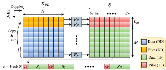
Figure 7: The CP addition in FCP OTFS in both delay-Doppler and time domains.

The RFCP OTFS configuration allows the exploitation of the CPs in OTFS unlike OFDM as explained in Subsection IV-E. For instance, the repeated data in the FCP can be used to provide diversity between the transmitted data symbols. Also, it can be used to reduce the guard interval dedicated for pilot [9] into half by locating the pilot at the end part of the delay-Doppler grid. An illustration is shown in Fig. 9 where the CP block in FCP OTFS is compared to the one in the proposed RFCP frame. For that, one pilot is inserted at the end of the delay index (i.e., $l=M-1$) so that it is copied in the full CP portion. After passing through the doubly dispersive channel, it is seen that the pilot spreads accordingly with the propagation environment which has $L=4$ taps. At the receiver side, the data block and the CP block in both FCP and RFCP OTFS systems are plotted and shown in Fig. 9. It is observed that the pilot in the data block spreads similarly in both configurations following the model in (18) as depicted in Fig. 9 (a). On the other hand, it is seen that the CP block in the FCP frame suffers from high inter-Doppler interference as shown in Fig. 9 (b). On the contrary, Fig. 9 (c) shows an intact CIR following the model in (18) where the appended reduced CP provides enough protection to secure the CP block in RFCP OTFS.

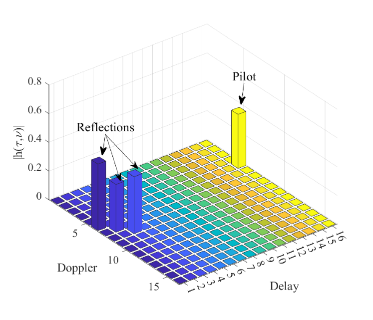
(a) The received signal after discarding CPs.

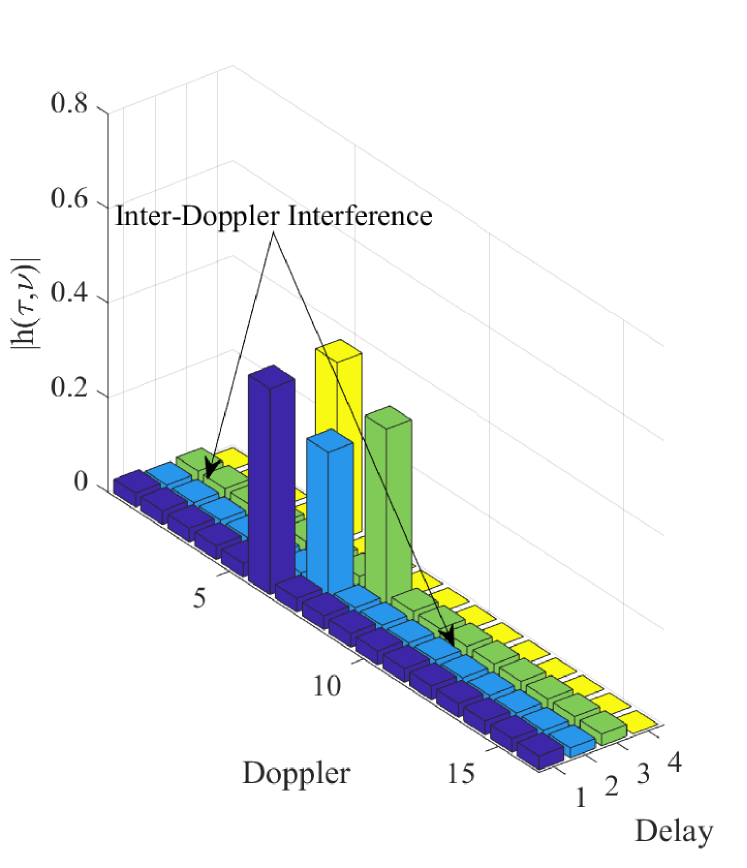
(b) The discarded CPs in FCP-OTFS.

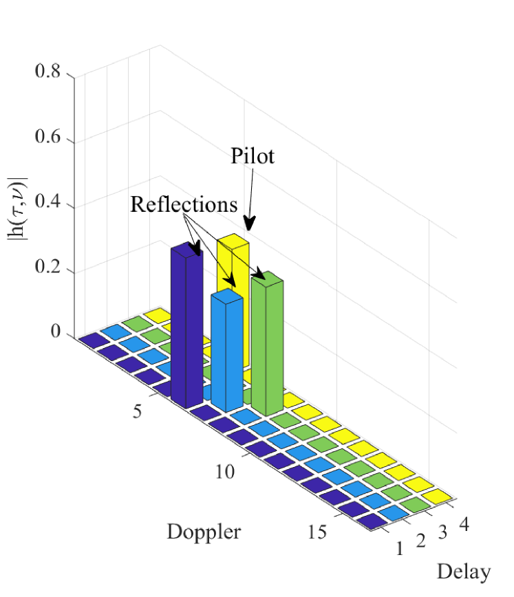
(c) The discarded CPs in RFCP-OTFS.

Figure 9: The delay-Doppler CIR of RFCP OTFS using $(M;N;L_{\mathrm{cp}})=(16,16,4)$. The number of paths in the delay-Doppler domain is $L=4$.

V Conclusion

In this paper, the input-output relation of OTFS systems has been analyzed when considering rectangular pulse shaping for RCP, RZP, FCP, and FZS prefixes and suffixes. It is shown that regardless of the prefix/suffix type used, the received signal model is similar except for the phase value corresponding the quasi-periodic shift in delay-Doppler domain. Consequently, it is concluded that channel estimation complexity, symbol detection performance are the same for all OTFS configurations. A novel mixed prefix type has been proposed where jointly reduced and full CP structures are appended to the OTFS frame, namely RFCP OTFS. In RFCP OTFS systems, the CP blocks are not discarded, and are being decoded along with data frame at the receiver side. Based on the application/need, the most appropriate prefix/suffix configuration has been defined to be adopted in the system model. In our future work, we will consider the effect of both fractional delay and Doppler in our model and accordingly we will analyze the different OTFS realizations under the new constraints.

Appendix A Proof of Theorem 1

A doubly-block circulant matrix is the outcome of the Kronecker product of two circulant matrices [28]. Let $\mathbf{C}_{1}\in\mathbb{C}^{N\times N},\mathbf{C}_{2}\in\mathbb{C}^{M\times M}$ be two circulant matrices and $\mathbf{A}\in\mathbb{C}^{MN\times MN}$, is the matrix resulting from the Kronecker product of $\mathbf{C}_{1}$ and $\mathbf{C}_{2}$ as follows

$$\mathbf{A} =\mathbf{C}_{1}\otimes\mathbf{C}_{2}.$$ (58)

Since $\mathbf{C}_{1}$ and $\mathbf{C}_{2}$ are circulant then they can be diagonalized using DFT matrices i.e., $\mathbf{F}_{N}^{-1}\mathbf{D}_{1}\mathbf{F}_{N}$ and $\mathbf{F}_{M}\mathbf{D}_{2}\mathbf{F}_{M}^{-1}$ [29]. Then,

$$\mathbf{A} =\left(\mathbf{F}_{N}^{-1}\mathbf{D}_{1}\mathbf{F}_{N}\right)\otimes\left(\mathbf{F}_{M}\mathbf{D}_{2}\mathbf{F}_{M}^{-1}\right)$$ (59)

$$=\left(\mathbf{F}_{N}^{-1}\otimes\mathbf{F}_{M}\right)\left(\mathbf{D}_{1}\otimes\mathbf{D}_{2}\right)\left(\mathbf{F}_{N}\otimes\mathbf{F}_{M}^{-1}\right).$$

Note that $\mathbf{D}_{1}\otimes\mathbf{D}_{2}$ is a diagonal matrix because the Kronecker product of two diagonal matrices is a diagonal matrix. Therefore,

$$\boldsymbol{\Sigma}=\left(\mathbf{D}_{1}\otimes\mathbf{D}_{2}\right)=\left(\mathbf{F}_{N}\otimes\mathbf{F}_{M}^{-1}\right)\mathbf{A}\left(\mathbf{F}_{N}^{-1}\otimes\mathbf{F}_{M}\right).$$ (60)

Appendix B Proof of (18)

Each received element in the RCP system is given as

$$Y^{\mathrm{R_{\mathrm{cp}}}}(l,k) =\sum_{\beta=0}^{MN-1}\mathbf{H}_{\mathrm{eff}}^{\mathrm{R_{\mathrm{cp}}}}(kM+l,\beta)\mathbf{x}(\beta)$$ (61)

$$=\sum_{l^{\prime}=0}^{M-1}\sum_{k^{\prime}=0}^{N-1}\mathbf{H}_{\mathrm{eff}}^{\mathrm{R_{\mathrm{cp}}}}(kM+l,k^{\prime}M+l^{\prime})X_{\mathrm{DD}}(l^{\prime},k^{\prime})$$

$$=\sum_{l^{\prime}=0}^{M-1}\sum_{k^{\prime}=0}^{N-1}X_{\mathrm{DD}}(l^{\prime},k^{\prime})\sum_{i=0}^{L-1}h_{i}\mathbf{T}^{(i)}(kM+l,k^{\prime}M+l^{\prime}).$$

Note that $\mathbf{T}^{(i)}(kM+l,k^{\prime}M+l^{\prime})$ is non-zeros only when $l^{\prime}-[l-l_{i}]_{M}=k^{\prime}-[k-k_{i}]_{N}=0$. Then, by substituting (17) in (61), we find

$$Y^{\mathrm{R_{\mathrm{cp}}}}(l,k)=\sum_{l^{\prime}=0}^{M-1}\sum_{k^{\prime}=0}^{N-1}X_{\mathrm{DD}}(l^{\prime},k^{\prime})\sum_{i=0}^{L-1}h_{i}\Lambda_{i}(l,k)e^{j2\pi\frac{k_{i}}{N}\frac{l-l_{i}}{M}}$$ (62)

$$~{}~{}~{}~{}~{}~{}~{}~{}~{}~{}~{}~{}~{}~{}~{}~{}~{}\cdot\delta\left(l^{\prime}-[l-l_{i}]_{M}\right)\delta\left(k^{\prime}-[k-k_{i}]_{N}\right)$$

$$=\sum_{i=0}^{L-1}h_{i}e^{j2\pi\frac{k_{i}}{N}\frac{l-l_{i}}{M}}\Lambda_{i}(l,k)X_{\mathrm{DD}}\left(\left[l-l_{i}\right]_{M},\left[k-k_{i}\right]_{N}\right),$$

where

$$\Lambda_{i}(l,k)=\begin{cases}1&l_{i}\leq l<M\\ e^{-j2\pi\frac{k}{N}}&0\leq l<l_{i}\end{cases}.$$ (63)

Appendix C Proof of (29)

The permutation matrix $\boldsymbol{\Pi}^{l_{i}}_{M}$ is an identity matrix with columns shifted by a value of $l_{i}$. Then, each element of this matrix can be found as

$$\boldsymbol{\Pi}^{l_{i}}_{M}(l^{\prime},k^{\prime})=\delta\left([l^{\prime}-k^{\prime}]_{M}-l_{i}\right).$$ (64)

Since $\boldsymbol{\Delta}^{k_{i},n}_{M}$ is a diagonal matrix, the $(l^{\prime},k^{\prime})$-th element of the of $\mathbf{H}_{n}^{\mathrm{F_{\mathrm{cp}}}}(l^{\prime},k^{\prime})$ is calculated as

$$\mathbf{H}_{n}^{\mathrm{F_{\mathrm{cp}}}}(l^{\prime},k^{\prime})=\sum_{i=0}^{L-1}h_{i}\boldsymbol{\Delta}^{k_{i},n}_{M}\left([l^{\prime}-l_{i}]_{M},k^{\prime}\right)$$ (65)

$$=\sum_{i=0}^{L-1}h_{i}z_{i}^{\left(n(M+L_{\mathrm{cp}})+L_{\mathrm{cp}}+l^{\prime}-l_{i}\right)}\cdot\delta\left([l^{\prime}-k^{\prime}]_{M}-l_{i}\right).$$

substituting (65) in (29) we find

$$\mathbf{G}^{\mathrm{F_{\mathrm{cp}}}}_{n}(l^{\prime},k^{\prime}) =\sum_{\alpha=0}^{N}\sum_{i=0}^{L-1}h_{i}z_{i}^{\left(\alpha(M+L_{\mathrm{cp}})+L_{\mathrm{cp}}+l^{\prime}-l_{i}\right)}e^{-j2\pi nk/N}$$ (66)

$$\cdot\delta\left([l^{\prime}-k^{\prime}]_{M}-l_{i}\right).$$

Appendix D Proof of (30)

The vectorized form of the received signal in (30) can be written as

$$\mathbf{Y}^{\mathrm{F_{\mathrm{cp}}}}=\sum_{\alpha=0}^{N-1}\mathbf{H}_{\alpha}\mathbf{X}_{\mathrm{DD}}\mathbf{f}_{\alpha}^{*}\mathbf{f}_{\alpha}^{T}=\sum_{\alpha=0}^{N-1}\mathbf{H}_{\alpha}\mathbf{X}_{\mathrm{DD}}\boldsymbol{\Pi}_{\alpha},$$ (67)

where $\boldsymbol{\Pi}_{\alpha}(l^{\prime},k^{\prime})=e^{j2\pi\alpha\frac{l^{\prime}-k^{\prime}}{N}}$.

$$Y^{\mathrm{F_{\mathrm{cp}}}}(l,k) =\sum_{\alpha=0}^{N-1}\sum_{l^{\prime}=0}^{M-1}\sum_{k^{\prime}=0}^{N-1}H_{\alpha}^{\mathrm{F_{\mathrm{cp}}}}\left[l,l^{\prime}\right]X_{\mathrm{DD}}\left[l^{\prime},k^{\prime}\right]\Omega_{\alpha}\left[k^{\prime},k\right]$$ (68)

$$=\sum_{\alpha=0}^{N-1}\sum_{l^{\prime}=0}^{M-1}\sum_{k^{\prime}=0}^{N-1}\bigg{[}\sum_{i=0}^{L-1}h_{i}z_{i}^{\left(\alpha(M+L_{\mathrm{cp}})+L_{\mathrm{cp}}+l-l_{i}\right)}\bigg{.}$$

$$~{}~{}~{}~{}~{}~{}~{}~{}~{}~{}~{}~{}~{}~{}\bigg{.}\cdot\delta\left([l-l^{\prime}]_{M}-l_{i}\right)\bigg{]}X_{\mathrm{DD}}\left[l^{\prime},k^{\prime}\right]e^{j2\pi\alpha\frac{k^{\prime}-k}{N}}$$

$$=\sum_{l^{\prime}=0}^{M-1}\sum_{k^{\prime}=0}^{N-1}X_{\mathrm{DD}}\left[l^{\prime},k^{\prime}\right]\sum_{i=0}^{L-1}h_{i}\cdot\delta\left([l-l^{\prime}]_{M}-l_{i}\right)$$

$$~{}~{}~{}~{}~{}~{}~{}~{}~{}~{}~{}\times\sum_{\alpha=0}^{N-1}e^{j2\pi k_{i}\frac{\left(\alpha(M+L_{\mathrm{cp}})+L_{\mathrm{cp}}+l-l_{i}\right)}{(M+L_{\mathrm{cp}})N}}e^{j2\pi\alpha\frac{k^{\prime}-k}{N}}$$

$$=\sum_{l^{\prime}=0}^{M-1}\sum_{k^{\prime}=0}^{N-1}X_{\mathrm{DD}}\left[l^{\prime},k^{\prime}\right]\sum_{i=0}^{L-1}h_{i}\cdot\delta\left([l-l^{\prime}]_{M}-l_{i}\right)$$

$$~{}~{}~{}~{}~{}~{}~{}~{}~{}~{}~{}~{}~{}~{}\times e^{\frac{2\pi k_{i}(L_{\mathrm{cp}}+l-l_{i})}{(M+L_{\mathrm{cp}})N}}\sum_{\alpha=0}^{N-1}e^{j2\pi\alpha\frac{k_{i}+(k^{\prime}-k)}{N}}.$$

In the absence of fractional Doppler $\sum_{\alpha=0}^{N-1}e^{j2\pi\alpha\frac{k_{i}+(k^{\prime}-k)}{N}}=\delta\left([k-k^{\prime}]_{N}-k_{i}\right)$. Then,

$$Y^{\mathrm{F_{\mathrm{cp}}}}(l,k) =\sum_{l^{\prime}=0}^{M-1}\sum_{k^{\prime}=0}^{N-1}X_{\mathrm{DD}}\left[l^{\prime},k^{\prime}\right]\sum_{i=0}^{L-1}h_{i}\cdot\delta\left([l-l^{\prime}]_{M}-l_{i}\right)$$ (69)

$$~{}~{}~{}~{}~{}~{}~{}~{}~{}~{}~{}~{}~{}~{}\delta\left([k-k^{\prime}]_{N}-k_{i}\right)e^{\frac{j2\pi k_{i}(L_{\mathrm{cp}}+l-l_{i})}{(M+L_{\mathrm{cp}})N}}$$

$$=\sum_{i=0}^{L-1}h_{i}e^{\frac{j2\pi k_{i}(L_{\mathrm{cp}}+l-l_{i})}{(M+L_{\mathrm{cp}})N}}X_{\mathrm{DD}}\left(\left[k-k_{i}\right]_{N},\left[l-l_{i}\right]_{M}\right).$$

Appendix E Proof of (40)

The elements of the lower triangular matrix of $\mathbf{L}_{\alpha}^{\mathrm{F_{\mathrm{zs}}}}$ can be computed as follows

$$\mathbf{L}_{\alpha}^{\mathrm{F_{\mathrm{zs}}}}(l^{\prime},k^{\prime})=\sum_{i=0}^{L-1}h_{i}\boldsymbol{\Delta}^{k_{i},n}_{M}\left(l^{\prime}-l_{i},k^{\prime}\right)$$ (70)

$$=\sum_{i=0}^{L-1}h_{i}z_{i}^{\left(\alpha M+l-l_{i}\right)}\cdot\delta\left(l^{\prime}-k^{\prime}-l_{i}\right).$$

substituting (70) in (39) we find

$$\boldsymbol{\Omega}^{\mathrm{F_{zs}}}_{n}(l^{\prime},k^{\prime}) =\sum_{\alpha=0}^{N}\sum_{i=0}^{L-1}h_{i}z_{i}^{(\alpha M+l-l_{i})}e^{-j2\pi nk/N}\cdot\delta\left(l^{\prime}-k^{\prime}-l_{i}\right).$$ (71)

Appendix F Proof of (41)

To derive the expression of the received signal $Y^{\mathrm{F_{zs}}}(l,k)$ in (41), we can follow the same steps in Appendix D by considering $L_{\mathrm{cp}}=0$ and $\mathbf{L}^{\mathrm{F_{zs}}}_{\alpha}$ instead of $\mathbf{H}^{\mathrm{F_{\mathrm{cp}}}}_{\alpha}$. Then, we find

$$Y^{\mathrm{F_{zs}}}(l,k) =\sum_{\alpha=0}^{N-1}\sum_{l^{\prime}=0}^{M-1}\sum_{k^{\prime}=0}^{N-1}L_{\alpha}^{\mathrm{F_{\mathrm{zs}}}}\left[l,l^{\prime}\right]X_{\mathrm{DD}}\left[l^{\prime},k^{\prime}\right]\Omega_{\alpha}\left[k^{\prime},k\right]$$ (72)

$$=\sum_{\alpha=0}^{N-1}\sum_{l^{\prime}=0}^{M-1}\sum_{k^{\prime}=0}^{N-1}\bigg{[}\sum_{i=0}^{L-1}h_{i}z_{i}^{\left(\alpha M+l^{\prime}\right)}\cdot\delta\left(l-l^{\prime}-l_{i}\right)\bigg{]}$$

$$~{}~{}~{}~{}~{}~{}~{}~{}~{}~{}~{}~{}~{}~{}\times X_{\mathrm{DD}}\left[l^{\prime},k^{\prime}\right]e^{j2\pi\alpha\frac{k^{\prime}-k}{N}}$$

$$=\sum_{l^{\prime}=0}^{M-1}\sum_{k^{\prime}=0}^{N-1}X_{\mathrm{DD}}\left[l^{\prime},k^{\prime}\right]\sum_{i=0}^{L-1}h_{i}\cdot\delta\left(l-l^{\prime}-l_{i}\right)$$

$$~{}~{}~{}~{}~{}~{}~{}~{}~{}~{}~{}~{}~{}~{}\delta\left([k-k^{\prime}]_{N}-k_{i}\right)e^{\frac{j2\pi k_{i}l^{\prime}}{MN}}$$

$$=\sum_{i=0}^{L-1}h_{i}e^{\frac{j2\pi k_{i}(l-l_{i})}{MN}}X_{\mathrm{DD}}\left(\left[k-k_{i}\right]_{N},l-l_{i}\right).$$

Note that $l-l_{i}$ is not modulo $M$ anymore. This because $\mathbf{L}_{\alpha}^{\mathrm{F_{\mathrm{zs}}}}$ is lower triangular matrix as proved in Appendix E.

References

• [1] G. Matz and F. Hlawatsch, “Fundamentals of time-varying communication channels,” in Wireless communications over rapidly time-varying channels.   Elsevier, 2011, pp. 1–63.
• [2] M. K. Ozdemir and H. Arslan, “Channel estimation for wireless ofdm systems,” IEEE Communications Surveys Tutorials, vol. 9, no. 2, pp. 18–48, Second Quarter 2007.
• [3] T. Yucek, R. M. Tannious, and H. Arslan, “Doppler spread estimation for wireless OFDM systems,” in IEEE/Sarnoff Symposium on Advances in Wired and Wireless Communication.   IEEE, 2005, pp. 233–236.
• [4] M. Yusuf and H. Arslan, “Controlled inter-carrier interference for physical layer security in OFDM systems,” in IEEE 84th Vehicular Technology Conference (VTC-Fall).   IEEE, 2016, pp. 1–5.
• [5] R. Hadani, S. Rakib, A. Molisch, C. Ibars, A. Monk, M. Tsatsanis, J. Delfeld, A. Goldsmith, and R. Calderbank, “Orthogonal time frequency space (OTFS) modulation for millimeter-wave communications systems,” in IEEE MTT-S International Microwave Symposium (IMS).   IEEE, 2017, pp. 681–683.
• [6] S. K. Mohammed, “Derivation of OTFS modulation from first principles,” IEEE Transactions on Vehicular Technology, vol. 70, no. 8, pp. 7619–7636, 2021.
• [7] P. Raviteja, Y. Hong, E. Viterbo, and E. Biglieri, “Practical pulse-shaping waveforms for reduced-cyclic-prefix OTFS,” IEEE Transactions on Vehicular Technology, vol. 68, no. 1, pp. 957–961, 2018.
• [8] G. Surabhi and A. Chockalingam, “Low-complexity linear equalization for OTFS modulation,” IEEE Communications Letters, vol. 24, no. 2, pp. 330–334, 2019.
• [9] P. Raviteja, K. T. Phan, and Y. Hong, “Embedded pilot-aided channel estimation for OTFS in delay–Doppler channels,” IEEE Transactions on Vehicular Technology, vol. 68, no. 5, pp. 4906–4917, 2019.
• [10] M. K. Ramachandran and A. Chockalingam, “MIMO-OTFS in high-Doppler fading channels: Signal detection and channel estimation,” in 2018 IEEE Global Communications Conference (GLOBECOM).   IEEE, 2018, pp. 206–212.
• [11] A. Tusha, S. Althunibat, M. O. Hasna, K. Qaraqe, and H. Arslan, “Exploiting User Diversity in OTFS Transmission for Beyond 5G Wireless Systems,” IEEE Wireless Communications Letters, 2022.
• [12] J. K. Francis, R. M. Augustine, and A. Chockalingam, “Diversity and PAPR Enhancement in OTFS using Indexing,” in IEEE 93rd Vehicular Technology Conference (VTC2021-Spring).   IEEE, 2021, pp. 1–6.
• [13] A. Tusha, S. Doğan-Tusha, F. Yilmaz, S. Althunibat, K. Qaraqe, and H. Arslan, “Performance Analysis of OTFS Under In-Phase and Quadrature Imbalance at Transmitter,” IEEE Transactions on Vehicular Technology, vol. 70, no. 11, pp. 11 761–11 771, 2021.
• [14] P. Singh, H. B. Mishra, and R. Budhiraja, “Low-complexity linear MIMO-OTFS receivers,” in IEEE International Conference on Communications Workshops (ICC Workshops).   IEEE, 2021, pp. 1–6.
• [15] N. Hashimoto, N. Osawa, K. Yamazaki, and S. Ibi, “Channel estimation and equalization for CP-OFDM-based OTFS in fractional doppler channels,” in IEEE International Conference on Communications Workshops (ICC Workshops).   IEEE, 2021, pp. 1–7.
• [16] V. Khammammetti and S. K. Mohammed, “OTFS-based multiple-access in high Doppler and delay spread wireless channels,” IEEE Wireless Communications Letters, vol. 8, no. 2, pp. 528–531, 2018.
• [17] P. Raviteja, E. Viterbo, and Y. Hong, “OTFS performance on static multipath channels,” IEEE Wireless Communications Letters, vol. 8, no. 3, pp. 745–748, 2019.
• [18] W. Shen, L. Dai, J. An, P. Fan, and R. W. Heath, “Channel estimation for orthogonal time frequency space (OTFS) massive MIMO,” IEEE Transactions on Signal Processing, vol. 67, no. 16, pp. 4204–4217, 2019.
• [19] T. Thaj and E. Viterbo, “Low complexity iterative rake decision feedback equalizer for zero-padded OTFS systems,” IEEE Transactions on Vehicular Technology, vol. 69, no. 12, pp. 15 606–15 622, 2020.
• [20] F. Liu, Z. Yuan, Q. Guo, Z. Wang, and P. Sun, “Multi-Block UAMP Based Detection for OTFS with Rectangular Waveform,” IEEE Wireless Communications Letters, 2021.
• [21] P. Raviteja, K. T. Phan, Y. Hong, and E. Viterbo, “Interference cancellation and iterative detection for orthogonal time frequency space modulation,” IEEE Transactions on Wireless Communications, vol. 17, no. 10, pp. 6501–6515, 2018.
• [22] P. Singh, K. Yadav, H. B. Mishra, and R. Budhiraja, “BER Analysis for OTFS Zero Forcing Receiver,” IEEE Transactions on Communications, vol. 70, no. 4, pp. 2281–2297, 2022.
• [23] R. Liu, Y. Huang, D. He, Y. Xu, and W. Zhang, “Optimizing Channel Estimation Overhead for OTFS with Prior Channel Statistics,” in IEEE Wireless Communications and Networking Conference (WCNC).   IEEE, 2021, pp. 1–6.
• [24] D. Wulich, “Definition of efficient PAPR in OFDM,” IEEE Communications Letters, vol. 9, no. 9, pp. 832–834, 2005.
• [25] S. E. Zegrar and H. Arslan, “Common CP-OFDM Transceiver Design for Low-Complexity Frequency Domain Equalization,” IEEE Wireless Communications Letters, 2022.
• [26] A. Farhang, A. RezazadehReyhani, L. E. Doyle, and B. Farhang-Boroujeny, “Low complexity modem structure for OFDM-based orthogonal time frequency space modulation,” IEEE Wireless Communications Letters, vol. 7, no. 3, pp. 344–347, 2017.
• [27] H. Qu, G. Liu, M. A. Imran, S. Wen, and L. Zhang, “Efficient Channel Equalization and Symbol Detection for MIMO OTFS Systems,” IEEE Transactions on Wireless Communications, 2022.
• [28] J. Calbert, L. Jacques, and P.-A. Absil, “Learning integral operators from diagonal-circulant neural networks,” Ph.D. dissertation, Master thesis. Université catholique de Louvain, 2020.
• [29] P. Davis, Circulant Matrices by Philip J. Davis, ser. Chelsea Publishing Series.   Chelsea, 1994. [Online]. Available: https://books.google.com.tr/books?id=BDgZwUSJSh8C