Molecular Gas Structures traced by ¹³CO Emission in the 18,190 ¹²CO Molecular Clouds from the MWISP Survey

Abstract

After the morphological classification of the 18,190 ¹²CO molecular clouds, we further investigate the properties of their internal molecular gas structures traced by the ¹³CO($J=$ 1$-$0) line emissions. Using three different methods to extract the ¹³CO gas structures within each ¹²CO cloud, we find that $\sim$ 15$\%$ of ¹²CO clouds (2851) have ¹³CO gas structures and these ¹²CO clouds contribute about 93$\%$ of the total integrated flux of ¹²CO emission. In each of 2851 ¹²CO clouds with ¹³CO gas structures, the ¹³CO emission area generally does not exceed 70$\%$ of the ¹²CO emission area, and the ¹³CO integrated flux does not exceed 20$\%$ of the ¹²CO integrated flux. We reveal a strong correlation between the velocity-integrated intensities of ¹²CO lines and those of ¹³CO lines in both ¹²CO and ¹³CO emission regions. This indicates the H₂ column densities of molecular clouds are crucial for the ¹³CO lines emission. After linking the ¹³CO structure detection rates of the 18,190 ¹²CO molecular clouds to their morphologies, i.e. nonfilaments and filaments, we find that the ¹³CO gas structures are primarily detected in the ¹²CO clouds with filamentary morphologies. Moreover, these filaments tend to harbor more than one ¹³CO structure. That demonstrates filaments not only have larger spatial scales, but also have more molecular gas structures traced by ¹³CO lines, i.e. the local gas density enhancements. Our results favor the turbulent compression scenario for filament formation, in which dynamical compression of turbulent flows induces the local density enhancements. The nonfilaments tend to be in the low-pressure and quiescent turbulent environments of the diffuse interstellar medium.

1 Introduction

Molecular clouds (MCs) are the fundamental forms of the molecular interstellar medium (ISM), which represent its coldest ($\sim$ 10 K), densest components (n $>$ 30 cm^-3) of the ISM. However, how molecular clouds form and what mechanisms determine their physical properties are still under debate. Previous studies have proposed several mechanisms, including large-scale gravitational instabilities (Lin & Shu, 1964; Goldreich & Lynden-Bell, 1965), agglomeration of smaller clouds (Oort, 1954; Field & Saslaw, 1965; Dobbs & Baba, 2014), turbulent flows (Vazquez-Semadeni et al., 1995; Passot et al., 1995; Ballesteros-Paredes et al., 1999a; Vázquez-Semadeni et al., 2006; Heitsch et al., 2006; Koyama & Inutsuka, 2002; Beuther et al., 2020). Understanding the mechanism by which molecular clouds form and evolve are crucial for comprehending star formation and galaxy evolution.

Molecular clouds usually present complex and hierarchical structures. Since its discovery by Wilson et al. (1970), CO line emission has been widely used as a tracer of molecular gas. The boundaries of MCs are usually defined by either the low-$J$ rotational CO emission or extinction above some threshold (Heyer & Dame, 2015). The unbiased Galactic plane CO survey, the Milky Way Imaging Scroll Painting (MWISP), is performed using the 13.7m millimeter-wavelength telescope of Purple Mountain Observatory (PMO) and observes ¹²CO, ¹³CO, and C¹⁸O $(J=1-0)$ spectra, simultaneously (Su et al., 2019). The first phase of the MWISP CO project covering the Galactic longitude from $l=9^{\circ}.75$ to $230^{\circ}.25$ and the Galactic latitude from $b=$ -5^∘.25 to 5^∘.25, has been completed. The second phase of MWISP has begun and intend to extend the Galactic latitude from $b=$ -10^∘.25 to 10^∘.25. This high-quality CO survey provides us with opportunities to promote the analysis of the molecular clouds properties to a large sample spanning wide spatial scales, different evolutionary stages and various environments.

After observations with sufficient sensitivity and high spatial resolution carried out using the Herschel telescope, filaments became known to play an important role in the star formation of MCs (André et al., 2010; Molinari et al., 2010; André et al., 2014, 2016; Yuan et al., 2019, 2020; Peretto et al., 2022). Our researchs in Yuan et al. (2021) (Paper I) use the 18,190 MCs identified by the ¹²CO lines data from MWISP survey and classfied them as filaments and nonfilaments. We found that the filaments make up about 10$\%$ of the total number of molecular clouds, while contributing about 90$\%$ of the total integrated flux of ¹²CO line emission. Despite the systematic difference between the filaments and nonfilaments in their spatial areas, their averaged H₂ column densities do not vary significantly. Neralwar et al. (2022a) have classified the SEDIGISM clouds into four morphologies and found that most of molecular clouds present elongated structures. In addition, the ringlike clouds show the peculiar properties, which are speculated to be related to the physical mechanisms that regulate their formation and evolution (Neralwar et al., 2022b). Following our paper I, several questions can be asked, for instance, is there any possible evolution sequence between filaments and nonfilaments? What are the physics behind the molecular clouds presenting filaments or nonfilaments? Quantifying the amount, distribution, and kinematics of the diffuse and dense gas among them may provide new clues to answering these questions.

Compared with the ¹²CO(1-0) line emission having a critical density of $\sim$ 10² cm^-3, the less abundant isotope ¹³CO(1-0) lines can trace the denser gas with a density of $\sim$ 10³ cm^-3. The large-scale, unbiased, and highly sensitive data on CO and its isotopic lines from the MWISP survey provides us with opportunities to systematically investigate the spatial distribution and properties of the diffuse and dense molecular gas in a large sample of Molecular clouds.

In this paper, we use the ¹³CO(1-0) line emission to trace relatively dense gas components within 18,190 ¹²CO molecular clouds and reveal the relationship between the ¹³CO gas fractions and morphologies in molecular clouds. In section 2, we describe the data set, including the ¹³CO line emission data and ¹²CO molecular cloud catalog; Section 3 introduces three different methods used to extract ¹³CO molecular gas structures in ¹²CO molecular clouds and compares their results. In Section 4, we present the distribution of the physical parameters of the extracted ¹³CO gas structures within the ¹²CO MCs and systematically investigate the correlation between ¹²CO(1-0) and ¹³CO(1-0) line emission in the ¹²CO clouds having ¹³CO structures, in addition, we also link the the ¹³CO gas structures and the morphologies of ¹²CO molecular clouds to reveal the possible relation between them. Section 5 discusses how our observational results provide the clues for us to understand the molecular clouds’ formation and evolution. We conclude with a summary in Section 6.

2 Data

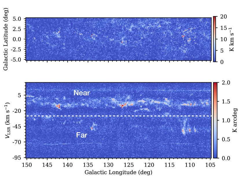
Figure 1: Top Panel: the velocity-integrated intensity map of ¹³CO(1-0) emission in the second Galactic quadrant with 104.75^∘ $<l<$ 150.25^∘ and $|b|<$ 5.25^∘. This map is derived by integrating the ¹³CO emission over the velocity range between -95 km s^-1 and 25 km s^-1. The distribution of noise RMS for the spectrum in each pixel is presented in Figure A1, the mean noise RMS is about 0.25 K. The sensitivity for this velocity-integrated map can be calculated as $\sigma\times\sqrt{N}\times dv$ = 1.2 K km/s, where $\sigma$ is the mean noise RMS (0.25 K), $dv$ represents the velocity resolution, its value is 0.17 km/s, $N=$ 760 is the number of the velocity channels. Bottom Panel: the latitude-integrated intensity map of ¹³CO(1-0) emission. This map is derived by integrating the ¹³CO emission over the latitude range from $-$5.25^∘ to 5.25^∘. The white dashed line at $V_{\rm LSR}=$ -30 km s^-1 divides the molecular clouds into two groups, i.e., the Near and Far groups, as described in Section 4.1. The velocity-integrated intensity maps and the latitude-integrated maps for the ¹³CO emission in the near and far velocity ranges, are shown in Figure A2 and A3, respectively.

2.1 ¹³CO $J=$ 1 – 0 data from MWISP survey

The ¹³CO data is from the MWISP survey, which is an ongoing northern Galactic plane CO survey. This survey is conducted by the 13.7m telescope at Delingha, China. The detailed introductions for the telescope, the multibeam receiver system, observation mode, and data reduction procedures are described in Su et al. (2019). The half-power beamwidth (HPBW) for the telescope at 115 GHz is about 50^′′. The velocity separation of ¹³CO lines is about 0.17 km s^-1. The main beam efficiency ($\eta_{\rm MB}$) varied between 40$\%$ and 50$\%$.

In this work, we focus on the ¹³CO emission in the Second Galactic Quadrant with $104^{\circ}.75<l<150^{\circ}.25$, $|b|<5^{\circ}.25$, and $-$95 km s^-1 $<$ V_LSR $<$ 25 km s^-1. Figure 1 presents the large-scale ¹³CO gas distribution as a velocity-integrated intensity map and a latitude-integrated intensity map.

2.2 Catalog and morphology classification

We define a molecular cloud as a contiguous structure in the position-position-velocity (PPV) data cube with ¹²CO(1-0) line intensities above a certain threshold. As described in Yan et al. (2021), a total of available 18,190 molecular clouds have been identified from the ¹²CO data cube in the range of $104^{\circ}.75<l<150^{\circ}.25$, $|b|<5^{\circ}.25$, and $-$95 km s^-1 $<$ V_LSR $<$ 25 km s^-1, using the Density-based Spatial Clustering of Applications with Noise (DBSCAN) algorithm (Ester et al., 1996; Yan et al., 2020).

In the paper I, we have compeleted the morphological classification for these ¹²CO molecular clouds, which are mainly classified into filaments and nonfilaments (Yuan et al., 2021). In this work, we aim to analyze the properties of high column density gas traced by the ¹³CO line emission in these molecular cloud samples.

3 Extracting ¹³CO $J=$ 1 – 0 Emission Structures within ¹²CO Molelcular Clouds

In this work, the ¹³CO emission structures are defined as molecular structures within the ¹²CO molecular clouds whose spectral voxels have the ¹³CO line intensities above a certain threshold. We utilize three different methods, i.e. clipping, DBSCAN (Ester et al., 1996; Yan et al., 2020), and moment mask (Dame, 2011) to extract the ¹³CO gas structures.

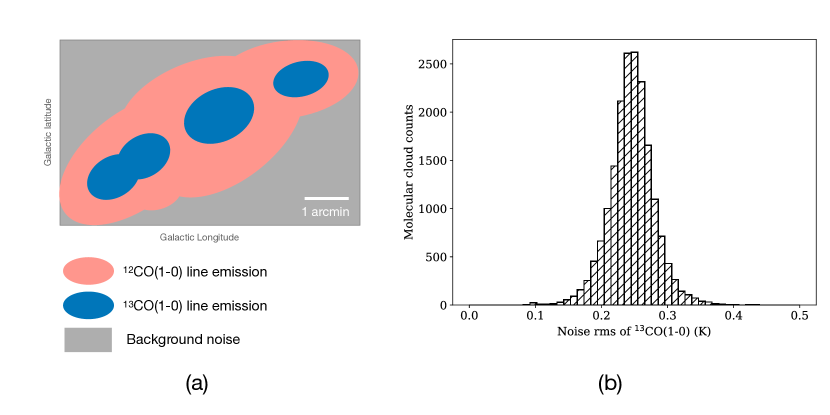
Figure 2: Panel (a): A cartoon demonstrating the distribution of ¹²CO molecular cloud, ¹³CO line emission, and the background region for estimating the RMS noise. Panel (b): The distribution of the RMS noise of the ¹³CO line for each molecular cloud.

3.1 Background noise

Before extracting the ¹³CO line emission within the ¹²CO molecular clouds, it is necessary to determine their RMS noises ($\sigma$). The ¹³CO spectral line data are chopped into the separate data cubes with sizes equivalent to the extent of ¹²CO emission in the PPV space for ¹²CO molecular clouds. Figure 2 presents a sketch map illustrating the distribution of ¹²CO molecular cloud, the ¹³CO emission structures, and the background noise in a separate data cube. The voxels within the background region in each ¹³CO data cube are utilized to estimate the RMS noise of ¹³CO lines for each molecular cloud. The distribution of the resultant ¹³CO rms noises for all of 18,190 molecular clouds are presented in Figure 2. The typical value is about 0.25 K. The corresponding RMS noise for each molecular cloud is used for the ¹³CO emission extraction. Furthermore, the values of voxels in the background region of each ¹³CO data cube are set to zeros, so that the ¹³CO structures are extracted within the ¹²CO emission boundaries. We extract the ¹³CO emission structures in these chopped 18,190 ¹³CO data cubes, which are correspond to the 18,190 ¹²CO molecular clouds.

3.2 Three methods

3.2.1 Clipping

Clipping is a common technique, which directly extracts the structures containing the ¹³CO spectral channels above the statistical significance level. Spectral channels in each ¹³CO data cube having intensities above the defined clipping levels are extracted as the significant ¹³CO emission. Whereas the clipping can not avoid the positive noise spikes with values above the clipping level, unless the clipping level is enough high. The high threshold used may lead to loss of the faint emission with intensities below the cutoff levels.

3.2.2 Moment Mask

The main point of a moment mask is that the ¹³CO emission is extracted on the smoothed ¹³CO spectral line data, to reduce the effects of noise spikes. The extracted structures are further extended to the adjacent voxels, whose ranges are determined by the smoothed spatial and velocity resolutions. The MWISP ¹³CO data has a spatial resolution of $\sim$ 50 arcsec and a velocity resolution of 0.17 km s^-1, we smooth the data with two times the beam size (FWHM_S $\sim$ 100^″) in position space and with four times the velocity channels in velocity space (FWHM_V $\sim$ 0.7 km s^-1).

In the smoothed ¹³CO data, we calculate the noise RMS ($\sigma_{\rm sm}$) and extract the ¹³CO emissions with intensities higher than the defined $\sigma_{\rm sm}$ levels. After that, the extracted ¹³CO structures are extended to the structures containing the voxels, which are adjacent to the extracted voxels. The adjacent voxels are defined as the ns pixels in spatially and nv pixels in velocity. Among that, ns = 0.5$\times$FWHM_S/ds, nv = 0.5$\times$FWHM_V/dv, ds and dv are the spatial and velocity resolutions for the raw data, respectively (Dame, 2011). According to the resolutions of the smoothed data, we obtain ns$=$1 and nv$=$2. Thus, a total of 3$\times$3$\times$5 voxels are determined to be adjacent to an extracted ¹³CO voxel. Based on the boundaries of enlarged structures, we obtain the determined ¹³CO structures from the raw ¹³CO data cube.

3.2.3 DBSCAN

DBSCAN algorithm, which was designed to discover clusters in arbitrary shape (Ester et al., 1996), has been developed to extract a set of contiguous voxels in the PPV space with ¹²CO emission above a certain threshold as a molecular cloud (Yan et al., 2020). This method is based on both the intensity levels and the connectivity of signals. We utilize the identical parameters to extract the ¹³CO emission as that used for the ¹²CO molecular clouds (Yan et al., 2020), except for the post-selection criteria of the peak values. For the ¹²CO emission, its peak intensity in a ¹²CO molecular cloud needs to be larger than the intensity of its boundary threshold adding 3$\sigma$. Owing to the relatively lower value for the ¹³CO line intensity, its peak intensity in a ¹³CO structure is larger than the intensity of its boundary threshold adding the 2$\sigma$, where $\sigma$ is the background noise. The parameters used for the DBSCAN extraction are described in detail in Appendix B. The chopped ¹³CO data cube without any smoothing procedures is used for identifying the ¹³CO structures by the DBSCAN algorithm.

3.3 Comparison among different methods

3.3.1 Test on a Case: G139.73

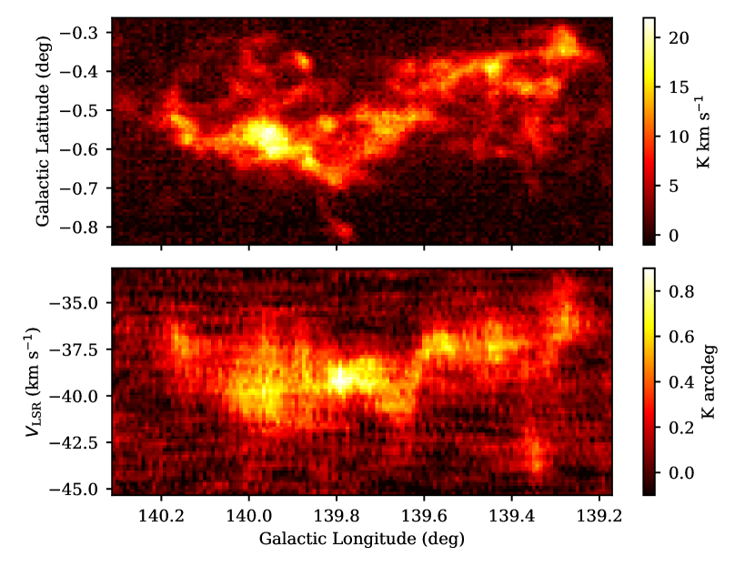
Figure C4: The velocity-integrated intensity map (upper) and latitude-integrated intensity map (lower) of ¹²CO emission for the molecular cloud G139.73, which are derivied by the raw chopped ¹²CO data cube without any clipping.

We take a ¹²CO molecular cloud G139.725-0.507-038.33 (hereafter G139.73) as an sample to compare the performances of the three different methods. In Figure C4 and C5, we present the velocity-integrated intensity maps and the latitude-integrated maps of ¹²CO and ¹³CO emission for the G139.73, which are integrated by the chopped data cubes without any clipping. Figure 3 shows the ¹³CO emission fluxes of the G139.73 extracted by three techniques at the cutoff levels from 2$\sigma$ to 10$\sigma$. We should note the noise $\sigma$ used by the moment mask is estimated using the smoothed data ($\sigma_{\rm sm}$ = 0.05 K), but that for the DBSCAN and clipping, their background noise $\sigma$ is calculated using the raw data without any smoothing procedures ($\sigma$ = 0.27 K). The distribution of integrated fluxes extracted by the DBSCAN and clipping algorithms have a similar trend and the values steep up from 4$\sigma$ to 2$\sigma$. For the moment mask with the noise $\sigma_{\rm sm}$ of 0.05 K, its extracted fluxes are higher than that from two other methods at the same cutoff levels.

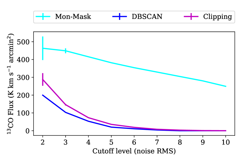
Figure 3: The distribution of ¹³CO emission fluxes within the ¹²CO cloud G139.73 extracted by three techniques at the cutoff levels from 2$\sigma$ to 10$\sigma$. The $\sigma$ for the clipping and DBSCAN is 0.27 K, which is calculated using the raw ¹³CO line data. Whereas the $\sigma$ for the moment mask is 0.05 K, estimated from the smoothed ¹³CO line data.

To quantify the contribution of the background noises to the ¹³CO emission fluxes using the three methods, we use a ¹³CO data cube without the significant ¹³CO emission to represent the pure background noises. Further, three methods are performed for the extraction of the ¹³CO line emission in this noise cube at the cutoff levels from 2$\sigma$ to 10$\sigma$. This noise data have the same sizes and spatial positions as that of the G139.73 data cube but in the different radial velocity range of (-90.3 -78.4) km s^-1. The extracted noise fluxes are shown as the error bars in Figure 3. We find that the background noises contribute about 15$\%$ of the integrated fluxes by the moment mask and clipping at the cutoff level of 2$\sigma$. Whereas, the DBSCAN almost completely avoids the background noise. We should note that these effects of the background noises on the integrated fluxes are based on a case of G139.73, whose ¹³CO line emissions have relatively high intensities. For the molecular clouds with faint emission and small spatial scales, the effects of noises can be magnified.

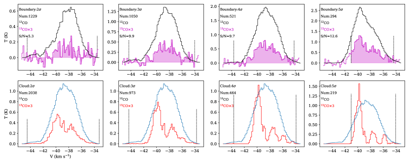
Figure C6: Upper panels: the mean spectrum of ¹²CO (black) and ¹³CO (magenta) spectral lines along the boundaries of ¹³CO structures extracted in the molecular cloud G139.73 by the clipping at the cutoff level of 2$\sigma$, 3$\sigma$, 4$\sigma$, and 5$\sigma$, respectively. The ¹³CO spectral lines are from the raw chopped ¹³CO data cube without any clipping, as shown in Figure C5. The ¹²CO spectral lines are from the extracted ¹²CO cloud of G139.73. The noted Num in each panel is the number of the spectrum along the corresponding boundary. The S/N is the ratio of the peak intensity to the noise RMS for the averaged-boundary ¹³CO spectrum. Lower panels: the mean spectrum of the extracted ¹²CO cloud (blue) in Yan et al. (2021) and the mean spectrum of the ¹³CO structures (red) extracted by the clipping at the cutoff level of 2$\sigma$, 3$\sigma$, 4$\sigma$, and 5$\sigma$. The vertical dashed lines illustrate the velocity span for the extracted ¹³CO structures within G139.73 by the clipping at the corresponding cutoff levels of 2$\sigma$, 3$\sigma$, 4$\sigma$, and 5$\sigma$, respectively. All the ¹³CO spectra are multiplied by a factor of 3. The $\sigma$ value is estimated from the raw data and equal to 0.27 K

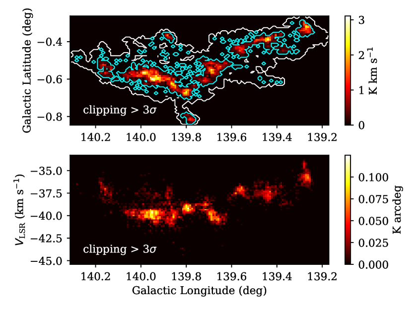
Figure C7: The velocity-integrated intensity map (upper) and latitude-integrated intensity map (lower) of ¹³CO emission extracted within the ¹²CO cloud G139.73 using the clipping at the cutoff level of 3$\sigma$ (0.81 K). The white contours are the boundaries of ¹²CO molecular cloud. The cyan contours are the determined boundaries of ¹³CO line emission.

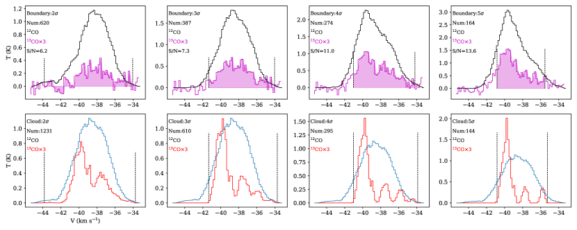
Figure C9: Same as Figure C6, but for the ¹³CO structures extracted by the DBSCAN algorithm at the cutoff level of 2$\sigma$, 3$\sigma$, 4$\sigma$, and 5$\sigma$.

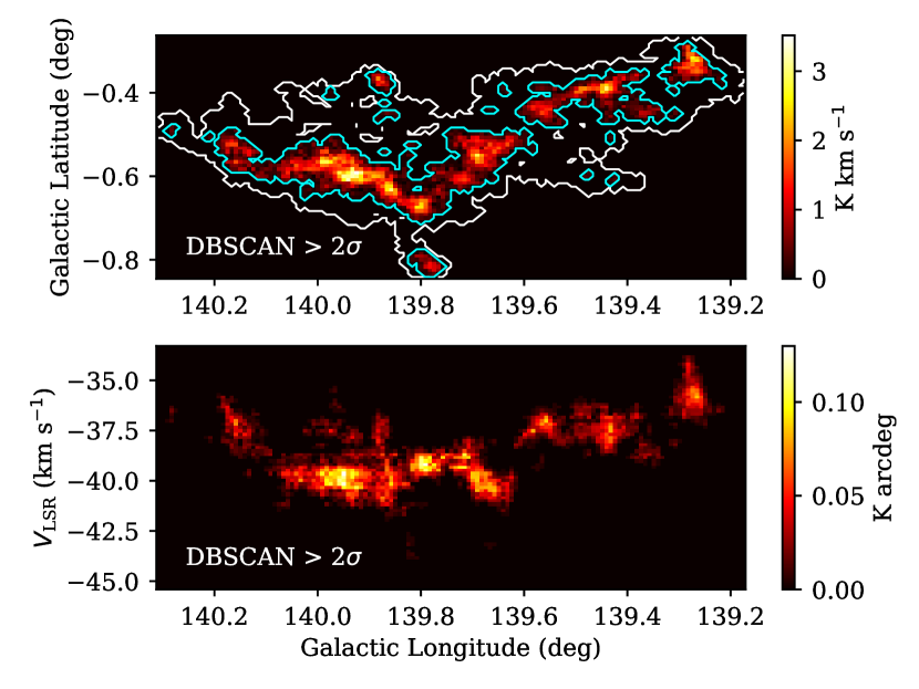
Figure C10: Same as Figure C7, but using the DBSCAN at the cutoff level of 2$\sigma$ (0.54 K).

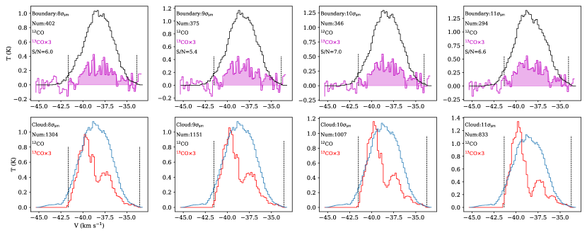
Figure C12: Same as Figure C6, but for the ¹³CO structures identified by the moment mask at the cutoff level of 8$\sigma_{\rm sm}$, 9$\sigma_{\rm sm}$, 10$\sigma_{\rm sm}$ and 11$\sigma_{\rm sm}$. The noise $\sigma_{\rm sm}$ is calculated from the smoothed data. Its value is 0.05 K.

In Figure C6, we present the averaged ¹²CO and ¹³CO spectral lines for pixels along the boundaries, which are determined by the clipping at the cutoff level from 2$\sigma$ to 5$\sigma$, as well as the corresponding mean ¹³CO spectral lines of the extracted ¹³CO structures. From the cutoff level of 3$\sigma$, the averaged ¹³CO spectrum along the determined boundary begins to have a significant signal. In Figure C7 and C8, we show the velocity-integrated map and latitude-integrated map of the extracted ¹³CO structures at cutoff level of 3$\sigma$ and 4$\sigma$. We find that there are a lot of positive spikes extracted by the clipping at the cutoff level of 3$\sigma$. The same spectral lines for the ¹³CO structures but extracted using the DBSCAN are presented in Figure C9. For the DBSCAN, the mean ¹³CO spectrum along its boundary determined at 2$\sigma$ begins to have a significant ratio of signal to noise (S/N). We also show the integrated maps of the extracted ¹³CO structures by the DBSCAN at the threshold of 2$\sigma$ and 3$\sigma$ in Figure C10 and C11. Figure C12 presents the same ¹³CO spectral lines for ¹³CO structures but identified using the moment mask at the cutoff level from 8$\sigma_{\rm sm}$ to 11$\sigma_{\rm sm}$. The averaged-boundary ¹³CO spectrum begins to show the effective signal at 9$\sigma_{\rm sm}$. The maps for the extracted ¹³CO structures by the moment mask at 8$\sigma_{\rm sm}$ and 9$\sigma_{\rm sm}$ are shown in Figure C13 and C14. We find that there are tiny ¹³CO structures extracted by the DBSCAN, not presented in the structures from the moment mask. We should note that the S/N for the averaged-boundary spectrum is related to the number of the spectrum along the boundaries. For the molecular clouds with smaller spatial scales, the averaged-boundary spectrum for ¹³CO structures extracted using the same method at the same threshold may not have a significant S/N. The cutoff levels of 4$\sigma$ for the clipping, 2$\sigma$ for the DBSCAN, and 9$\sigma_{\rm sm}$ for the moment mask are adopted to extract the ¹³CO structures.

Table 1: The number detection rates, area ratios, and the total flux ratios between the ¹³CO and ¹²CO line emission from three methods.

Methods	Number detection rates	Area ratios	Flux ratios
Clipping	13.5$\%$	10.8$\%$	4.1$\%$
DBSCAN	15.7$\%$	20.3$\%$	6.3$\%$
Monment Mask	15$\%$	20.7$\%$	7.3$\%$

Note. — The number detection rate is the number of ¹²CO clouds having ¹³CO structures divided by the total number of 18,190. The area ratio is the ratio between the total angular areas of the extracted ¹³CO structures and the total ¹²CO angular areas of 18,190 ¹²CO clouds. The flux ratio is the total integrated fluxes of the extracted ¹³CO line emission divided by that of ¹²CO line emission.

3.3.2 Number detection rate

We determine to extract the ¹³CO structures within a large sample of ¹²CO molecular clouds, which have the angular areas spanning from 1 to 10⁴ arcmin² and the integrated fluxes ranging from $\sim$ 1 to 10⁵ K km s^-1 arcmin², using the clipping at the cutoff of 4$\sigma$, the DBSCAN at the cutoff of 2$\sigma$, and the moment mask by a threshold of 9$\sigma_{\rm sm}$, to compare the extracted results from the three different methods.

For the clipping, there are 4,390 molecular clouds detected ¹³CO line emission. The extracted structure with values above the threshold, whose spatial size is one pixel (0.25 arcmin) or its velocity span is just one channel (0.17 km s^-1), is determined as the noise spike. After removing these noise spikes, 2,462 molecular clouds are regarded as having the significant ¹³CO line emission. However, the DBSCAN and Moment mask algorithms do not extract individual noise spike. For the DBSCAN algorithm, 2,851 molecular clouds are identified to have the ¹³CO emission. The moment mask extracts the ¹³CO line emission in the 2,735 molecular clouds. The number detection rates in the total 18,190 MCs by three methods are listed in Table 1.

3.3.3 Area ratios between the ¹³CO and ¹²CO line emission

The total angular area for the 18,190 ¹²CO molecular clouds is about 228.2 deg². The total angular area for the extracted ¹³CO structures within the 18,190 ¹²CO clouds by the clipping is 24.7 deg². The value is 46.2 deg² extracted by the DBSCAN and 47.2 deg² from the moment mask. The ratios between the total ¹³CO angular areas of the extracted ¹³CO structures and the total ¹²CO angular areas of the 18,190 ¹²CO clouds are listed in Table 1.

3.3.4 Integrated flux ratios between the ¹³CO and ¹²CO line emission

The total ¹²CO(1-0) emission fluxes for the 18,190 ¹²CO molecular clouds is 3.7$\times$10⁶ K km s^-1 arcmin². The total extracted ¹³CO(1-0) emission flux in this catalog is 1.5$\times$10⁵ K km s^-1 arcmin² by the clipping. The value is 2.3$\times$10⁵ K km s^-1 arcmin² by the DBSCAN algorithm and 2.7$\times$10⁵ K km s^-1 arcmin² by the moment mask method. These total integrated flux ratios between the ¹³CO and ¹²CO line emission by three methods are listed in Table 1.

We find that the number detection rates of the DBSCAN and moment mask are consistent with $\sim$ 15$\%$, the value of the clipping is about 2$\%$ lower than that of the other two techniques. In addition, the clipping extracts plenty of positive noise spikes. For the total angular areas of the extracted ¹³CO structures, the values from the clipping is about 50$\%$ of that from the DBSCAN and moment mask. For the extracted integrated fluxes of ¹³CO line emission, the values from the clipping are about 60$\%$ of that from the DBSCAN or Moment mask. That indicates the clipping method extracts amounts of noise spikes with intensities larger than the threshold of 4$\sigma$, meanwhile, it also loses substantial faint ¹³CO emission. For either the total angular areas or the total integrated fluxes of the extracted ¹³CO structures, the values from the moment mask are a bit higher than that from the DBSCAN, while the number detection rate of the moment mask is a bit lower than that from the DBSCAN. Overall, these values from the DBSCAN and moment mask are close.

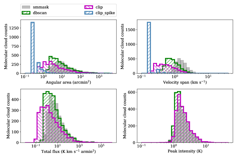
Figure 4: The number distributions of angular sizes, mean velocity spans, the integrated fluxes of ¹³CO line emission, and the peak intensities of ¹³CO(1-0) line emission for the ¹³CO structures extracted by three techniques. For the clipping, the extracted ¹³CO emission structures with a pixel in spatial scale or a velocity channel in velocity, are determined as the noise spikes and shown as blue histograms.

3.3.5 Differences of extracted basic parameters

The ¹³CO emissions are extracted within the ¹²CO clouds by three methods. All the ¹³CO emissions within the boundary of a ¹²CO cloud belong to the same cloud. We take all the ¹³CO line emissions within a ¹²CO cloud as a whole, referred to as ¹³CO molecular gas structures. The equivalent angular area of ¹³CO molecular structures ($\mathcal{A}_{\rm{}^{13}CO}$) for a ¹²CO cloud is the sum of the pixel areas of the extracted ¹³CO emission regions projected in the l-b panel. The mean velocity span of ¹³CO molecular structures ($V_{\rm aver,^{13}CO}$) within a ¹²CO cloud is the averaged extracted velocity span of each pixel in the ¹³CO emission regions, weighting by its corresponding velocity-integrated intensity, i.e. $V_{\rm aver,^{13}CO}=\Sigma(V_{\rm span}(l,b)\times W_{\rm{}^{13}CO}(l,b))/\Sigma W_{\rm{}^{13}CO}(l,b)$. The total ¹³CO integrated flux ($F_{{}^{13}CO}$) is the integrated flux of all the ¹³CO structures in an individual molecular cloud, $F_{\rm{}^{13}CO}$ = $\int$T${}_{\rm mb}(l,b,v)dldbdv$ = 0.166$\times$0.25$\Sigma$T${}_{\rm mb}(l,b,v)$ K km s^-1 arcmin², where $T_{\rm mb}(l,b,v)$ is the ¹³CO line intensity at the coordinate of $(l,b,v)$ in PPV space, $dv=$ 0.166 km s^-1 is the velocity resolution. The peak value ($T_{\rm{peak},^{13}CO}$) is the maximal value of the ¹³CO line intensities for the extracted ¹³CO structures.

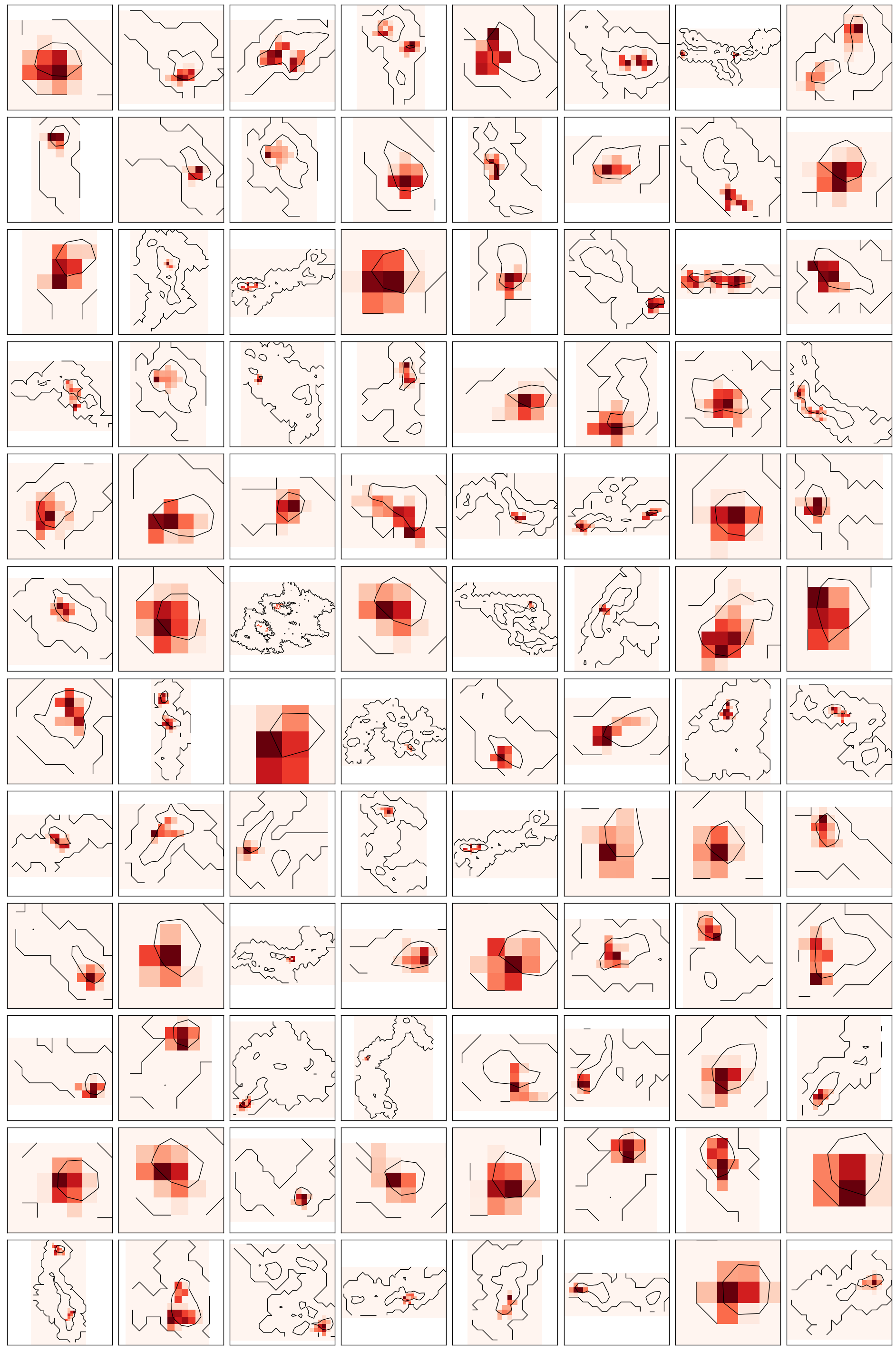
Figure D15: ¹³CO structures identified by the DBSCAN, but not by the moment mask. The colormaps represent the distributions of the velocity-integrated intensities of ¹³CO line emission. The black contours indicate the boundaries and the level of 50$\%$ at the ¹²CO line velocity-integrated intensities.

The number distributions of angular sizes ($\mathcal{A}_{\rm{}^{13}CO}$), mean velocity spans ($V_{\rm{aver},^{13}CO}$), integrated fluxes ($F_{{}^{13}CO}$), and peak intensities ($T_{\rm{peak},^{13}CO}$) of ¹³CO structures, which are identified by three techniques, are presented in Figure 4. We find the angular sizes of ¹³CO structures extracted by the clipping are systematically smaller than that from the DBSCAN and moment mask. We compare the angular sizes of ¹³CO structures from the DBSCAN and moment mask, their distributions in the range of the angular sizes larger than 6 arcmin² are similar. There are more structures from the DBSCAN in the range of 1 – 6 arcmin². To check the reliability of these extra structures, which are identified by the DBSCAN, but not by the moment mask, we present their ¹³CO line intensity maps integrated along with three different directions ($l,b,v$) and their averaged ¹³CO line spectra. As shown in Figure D15, we find that these structures usually are located around the regions contoured at the levels of half of the peak velocity-integrated intensity of ¹²CO emission. In addition, their ¹³CO spectral profiles usually present the Gaussian-like profiles. Thus, we determine these ¹³CO structures are valid. The number distributions of $T_{\rm{peak},^{13}CO}$ of ¹³CO line emission from the three techniques are similar in the range of $T_{\rm{peak},^{13}CO}>$ 2.0 K. After the smooth procedure, a portion of tiny structures with $T_{\rm{peak},^{13}CO}<$ 2.0 K may be missed by the moment mask. For the distribution of the mean velocity span of ¹³CO structures, we find the values from the moment mask tend to be larger than that from the DBSCAN, and the values from the DBSCAN are prone to be larger than that from the clipping. That may be due to that the extracted voxels in the smoothed data by the moment mask are further extended to the adjacent voxels, while the intensities of voxels extracted by the DBSCAN are larger than 2$\sigma$, and the ¹³CO structures from the clipping only contain the velocity channels with intensities larger than 4$\sigma$. Thus the velocity span of ¹³CO emission in each spatial pixel is derived from the velocity channels with intensities larger than 2$\sigma$ for the DBSCAN and 4$\sigma$ for the clipping. The number distributions of $F_{\rm{}^{13}CO}$ have a similar trend with that of $\mathcal{A}_{\rm{}^{13}CO}$. That means the differences of the $F_{\rm{}^{13}CO}$ distributions from three techniques are mainly attributed to their $\mathcal{A}_{\rm{}^{13}CO}$ distributions.

3.4 Summary of methods

Above all, the clipping extracts plenty of noise spikes with values larger than 4$\sigma$ and meanwhile loses the faint significant emission having intensities less than 4$\sigma$. That leads to the extracted parameters being systematically smaller than that from the other two methods. In addition, the moment mask leaves out a part of faint and tiny ¹³CO structures, owing to the smooth procedure. The moment mask is more suitable for the structures with relative large angular sizes and high emission intensities. The DBSCAN algorithm can not only avoid the noise spikes but also preserve the faint and tiny ¹³CO structures not identified by the moment mask. Each voxel in the PPV space of the structures extracted by the DBSCAN is larger than 2$\sigma$. We take the resultant ¹³CO structures from the DBSCAN, which is consistent with the extraction algorithm used for the ¹²CO clouds identification, for the follow-up analysis.

Table 2: A catalog of ¹³CO line emission parameters

Name	$l_{\rm cen}$	$b_{\rm cen}$	$V_{\rm LSR}$	$\mathcal{A}_{\rm{}^{12}CO}$	$V_{\rm{span},^{12}CO}$	$T_{\rm{peak},^{12}CO}$	$F_{\rm{}^{12}CO}$	$\mathcal{A}_{\rm{}^{13}CO}$	$V_{\rm{span},^{13}CO}$	$T_{\rm{peak},^{13}CO}$	$F_{\rm{}^{13}CO}$
	(degree)	(degree)	(km s-1)	(arcmin2)	km s-1	(K)	(K km s-1 arcmin2)	(arcmin2)	km s-1	(K)	(K km s-1 arcmin2)
G104.794+02.286-063.40	104.794	02.286	-63.40	03.50	01.67	2.95	4.40	01.50	01.16	0.99	0.55
G104.803-02.869-004.14	104.803	-2.869	-4.14	17.75	02.67	5.30	40.34	04.00	01.00	1.26	1.15
G104.810+01.058-009.45	104.810	01.058	-9.45	12.50	03.51	4.55	20.54	04.00	01.00	1.72	2.09
G104.822-02.335-034.52	104.822	-2.335	-34.52	11.75	04.01	5.14	38.85	02.75	01.33	1.11	0.70
G104.870-00.447-009.32	104.870	-0.447	-9.32	42.25	05.68	6.70	131.49	07.25	01.33	1.44	2.80
G104.871+00.646-001.89	104.871	00.646	-1.89	46.00	02.67	5.59	86.97	02.50	01.00	1.01	0.63
G104.872+01.008-049.95	104.872	01.008	-49.95	33.25	04.84	4.40	68.78	04.25	01.66	1.18	1.83
G104.886+00.134-010.58	104.886	00.134	-10.58	28.25	03.51	8.71	86.43	04.00	01.16	1.47	1.50
G104.923-03.111-046.89	104.923	-3.111	-46.89	04.25	02.00	6.59	9.49	02.00	00.83	1.50	0.88
G104.935+04.396-044.62	104.935	04.396	-44.62	07.25	02.34	5.90	16.76	03.50	01.16	1.40	1.48
G104.980+00.900-055.53	104.980	00.900	-55.53	19.50	03.51	4.43	30.89	02.50	00.83	1.10	0.62
G104.983-02.680-042.49	104.983	-2.680	-42.49	60.75	06.68	5.95	185.27	03.25	01.83	1.32	1.69
G104.997-02.669-004.75	104.997	-2.669	-4.75	26.25	04.34	6.56	79.88	07.25	01.66	1.69	2.78
G105.023+00.538-049.82	105.023	00.538	-49.82	44.25	04.51	6.06	159.96	19.25	01.83	2.61	14.01

Note. — The central Galactic coordinates ($l_{\rm cen}$, $b_{\rm cen}$) for each ¹²CO cloud are the averaged Galactic coordinates in its velocity-integrated ¹²CO(1-0) intensity map, weighting by the value of the velocity-integrated ¹²CO(1-0) intensity. The central velocity ($V_{\rm LSR}$) for each cloud is the averaged radial velocity in its radial velocity field, weighting by the value of the velocity-integrated ¹²CO(1-0) intensity. The $\mathcal{A}_{\rm{}^{12}CO}$ and $\mathcal{A}_{\rm{}^{13}CO}$ are the angular areas of ¹²CO(1-0) and ¹³CO(1-0) lines emission, respectively. The $V_{\rm{span},^{12}CO}$ represents the velocity span of each cloud cube in the velocity axis of PPV space, which is calculated using the number of velocity channels in the ¹²CO cloud cube multiplied by a velocity resolution of 0.167 km s^-1. The $V_{\rm{span},^{13}CO}$ is the velocity range between the maximal and minimal velocity for all the extracted ¹³CO gas structures within each ¹²CO molecular cloud. The $T_{\rm{peak},^{12}CO}$ and $T_{\rm{peak},^{13}CO}$ represent the peak values of ¹²CO(1-0) and ¹³CO(1-0) line intensity in each cloud, respectively. The $F_{\rm{}^{12}CO}$ is the integrated flux of ¹²CO(1-0) line emission for each cloud, $F_{\rm{}^{12}CO}$ = $\int$T${}_{\rm mb}(l,b,v)dldbdv$ = 0.167$\times$0.25$\Sigma$T${}_{\rm mb}(l,b,v)$ K km s^-1 arcmin², where $T_{\rm mb}(l,b,v)$ is the ¹²CO line intensity at the coordinate of $(l,b,v)$ in PPV space, $dv=$ 0.167 km s^-1 is the velocity resolution, $dldb=$ 0.5 arcmin $\times$ 0.5 arcmin $=$ 0.25 arcmin², the angular size of a pixel is 0.5 arcmin. The $F_{\rm{}^{13}CO}$ is calculated using the ¹³CO(1-0) line emission within each cloud through the same formula, but T${}_{\rm mb}(l,b,v)$ is the ¹³CO line intensity. This table is available in its entirety from the online journal. A portion is shown here for guidance regarding its form and content.

4 Results

4.1 Comparing the physical properties of molecular clouds with and without ¹³CO molecular structures

The whole catalog of 18,190 molecular clouds is identified using the ¹²CO(1-0) line data by the DBSCAN algorithm (Yan et al., 2021). Among that, the 2,851 ¹²CO clouds have ¹³CO structures, which are also extracted by the DBSCAN algorithm. Since the boundary of a molecular cloud is defined by the 3D surface of ¹²CO(1-0) line emission in the PPV space, all the ¹³CO emissions within this surface belong to the same ¹²CO cloud. Thus its internal ¹³CO emission components are characterized as its substructures, which are referred to as ¹³CO molecular structures. All the extracted ¹²CO(1-0) line emission data of 18,190 molecular clouds and the extracted ¹³CO(1-0) line emission data within the 2,851 ¹²CO clouds have been published in ScienceDB (Yuan et al., 2022).

We should note that a single molecular cloud may have more than one individual ¹³CO molecular structure. We take all the separate ¹³CO molecular structures in a single ¹²CO molecular cloud as a unity. The ¹³CO emission parameters are derived from all the ¹³CO structures in a ¹²CO cloud as a whole. The equivalent angular area of ¹³CO molecular structures for a ¹²CO cloud is the sum of the pixel areas of the extracted ¹³CO emission regions projected in the l-b panel. The velocity span of ¹³CO molecular structures within a ¹²CO cloud is the range between the maximal and minimal velocity of the extracted ¹³CO structures along the velocity axis. For a ¹²CO cloud with multiple ¹³CO structures, the minimal velocity is the minimal value in the velocity ranges for all the extracted ¹³CO structures and the maximal velocity is the maximal value of that. Figure C9 illustrates the velocity span for the extracted ¹³CO structures in the ¹²CO cloud G139.73. The ¹³CO integrated fluxes are the integrated fluxes of all the ¹³CO structures in an individual molecular cloud. The peak value is the maximal value of the ¹³CO line intensities within the boundary of a ¹²CO MC. The parameters of ¹³CO molecular structures for the 2,851 ¹²CO molecular clouds are listed in Table 2. The rest 15,339 ¹²CO molecular clouds do not have the significant ¹³CO structures. We systematically compare the basic physical parameters of the ¹²CO molecular clouds having ¹³CO structures (¹³CO-detects) to that of molecular clouds without ¹³CO structures (Non¹³CO-detects).

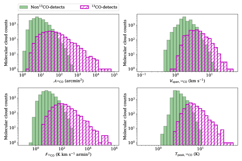
Figure 5: The number distributions of angular areas ($\mathcal{A}_{\rm{}^{12}CO}$), velocity spans ($V_{\rm{span,^{12}CO}}$), the peak intensities ($T_{\rm{peak,^{12}CO}}$) and the integrated fluxes ($F_{\rm{}^{12}CO}$) of ¹²CO line emission for ¹²CO molecular clouds with and without ¹³CO structures. The green histgrams represent ¹²CO molecular clouds not having the ¹³CO structures (Non¹³CO-detects). The magenta ones are the ¹²CO molecular clouds having the ¹³CO structures (¹³CO-detects).

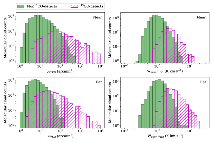
Figure 6: The number distributions of angular areas ($\mathcal{A}_{\rm{}^{12}CO}$) and the averaged velocity-integrated intensities ($W_{\rm{aver,^{12}CO}}$) of ¹²CO line emission for ¹²CO molecular clouds in near and far groups, respectively. The near ¹²CO clouds are in a velocity range of (-30 25) km s^-1, the far ¹²CO clouds are in (-95 -30) km s^-1. The green histgrams represent ¹²CO molecular clouds not having the ¹³CO structures (Non¹³CO-detects). The magenta ones are the ¹²CO molecular clouds having the ¹³CO structures (¹³CO-detects).

In Figure 5, we present the number distributions of angular areas ($\mathcal{A}_{\rm{}^{12}CO}$), velocity spans ($V_{\rm{span},^{12}CO}$), peak intensities ($I_{\rm{peak},^{12}CO}$), and integrated fluxes ($F_{\rm{}^{12}CO}$) of ¹²CO line emission for the ¹³CO-detects and Non¹³CO-detects, respectively. The quantiles at 0.05, 0.25, 0.5, 0.75, and 0.95 of these parameters for the ¹³CO-detects and Non¹³CO-detects are listed in Table 3, respectively. We find that these quantiles of the parameters in the ¹³CO-detects are systematically larger than that from the Non¹³CO-detects. We calculate the total $F_{\rm{}^{12}CO}$ of the whole Non¹³CO-detects. The value is about 2.5$\times$10⁵ K km s^-1 arcmin², which makes up about 6.8$\%$ of that of the total 18,190 ¹²CO molecular clouds (3.7$\times$10⁶ K km s^-1 arcmin²). The rest $\sim$ 93$\%$ are from the ¹³CO-detects. That indicates the ¹³CO-detects are the main contributor of ¹²CO emission fluxes, although their number only take a percentage of $\sim$ 15$\%$ in the total number. The total $\mathcal{A}_{\rm{}^{12}CO}$ for the 18,190 ¹²CO clouds is about 228.2 deg². Among that, the sum of the $\mathcal{A}_{\rm{}^{12}CO}$ from the ¹³CO-detects take a percentage of 76.2$\%$ and that from the Non¹³CO-detects take about the rest of 23.8$\%$.

Table 3: The physical parameters of ¹²CO line emission for Non¹³CO-detects and ¹³CO-detects

Types	Quantile	$\mathcal{A}_{\rm{}^{12}CO}$	$V_{\rm span,^{12}CO}$	$T_{\rm{peak},^{12}CO}$	$F_{{}^{12}CO}$
		(arcmin2)	(km s-1)	(K)	(K km s-1 arcmin2)
	0.05	2.5	1.0	2.2	1.7
	0.25	4.25	1.5	2.5	3.9
Non13CO-detects	0.5	7.25	2.0	2.9	7.6
	0.75	13.75	2.67	3.5	16.6
	0.95	39.5	4.2	5.0	58.8
	Mean	12.8	2.2	3.1	16.5
	0.05	6.25	1.84	3.8	11.8
	0.25	16.4	2.84	5.1	38.9
13CO-detects	0.5	39	4.0	6.3	101.2
	0.75	102.5	5.68	8.3	299.4
	0.95	640.0	10.35	13.3	2422.3
	Mean	219.5	4.73	7.3	1211.9

Note. — The quantiles at 0.05, 0.25, 0.5, 0.75 and 0.95 for each parameter in its sequential data and its mean value.

Table 4: The angular areas ($\mathcal{A}_{\rm{}^{12}CO}$) and H₂ column densities (N${}_{\rm H_{2}}$) for ¹³CO-detects and Non¹³CO-detects, which are in the near and far groups, respectively.

Types	Quantile	$\mathcal{A}_{\rm{}^{12}CO}$	N${}_{\rm H_{2}}$
		(arcmin2)	1020 cm-2
		Near, Far	Near, Far
	0.05	2.5, 2.25	1.05, 1.2
	0.25	5.0, 3.75	1.46, 1.72
Non13CO-detects	0.5	8.5, 6.0	1.88, 2.2
	0.75	16.75, 10.75	2.5, 2.88
	0.95	51.1, 26.5	3.9, 4.26
	Mean	15.6, 9.1	2.1, 2.4
	0.05	8.5, 5.75	2.4, 2.8
	0.25	31.88, 13.25	3.5, 4.1
13CO-detects	0.5	73.13, 28.75	4.6, 5.4
	0.75	185.13, 70.0	6.2, 7.48
	0.95	1134.4, 322.5	9.6, 13.3
	Mean	413.8, 116.3	5.2, 6.4

Note. — The quantiles at 0.05, 0.25, 0.5, 0.75 and 0.95 for the $\mathcal{A}_{\rm{}^{12}CO}$ and N${}_{\rm H_{2}}$ in their sequential data and their mean values. The H₂ column density (N${}_{\rm H_{2}}$) are calculated using the N${}_{\rm H_{2}}$ = X_COW${}_{\rm{}^{12}CO}$, where X_CO=2$\times$10²⁰ cm^-2 (K km s^-1)^-1. The Near represents the molecular clouds in the near range ($V_{\rm LSR}$ from $-$30 km s^-1 to 25 km s^-1), the Far means the molecular clouds in the far range ($V_{\rm LSR}$ from $-$95 km s^-1 to $-$30 km s^-1).

Following the paper I (Yuan et al., 2021), the ¹²CO clouds are divided into two groups by a $V_{\rm LSR}$ threshold of - 30 km s^-1, shown as a white-dashed line in Figure 1. The ¹²CO clouds with central velocities in a range of (-30 25) km s^-1 are in the near group, and the ¹²CO clouds with central velocities ranging from -95 km s^-1 to -30 km s^-1 are in the far group. In the near group, there are 9,544 ¹²CO molecular clouds, among which the ¹³CO-detects take a percentage of 10.4$\%$. In the far group, there are 8,646 ¹²CO molecular clouds and 21.5$\%$ of them have ¹³CO structures.

The number detection rate of the ¹³CO-detects in the near is lower than that in the far group. That may be due to that there are more MCs with faint ¹²CO emission, but no ¹³CO emission detected in the near group. The number distributions of the $\mathcal{A}_{\rm{}^{12}CO}$ of ¹³CO-detects and Non¹³CO-detects in the near and far group are presented in Figure 6, respectively. The quantiles at 0.05, 0.25, 0.5, 0.75, and 0.95 of their $\mathcal{A}_{\rm{}^{12}CO}$ values are listed in Table 4. According to the spiral structure of the Milky Way, the kinematical distances, which are estimated using the Bayesian distance calculator in Reid et al. (2016), center on about $\sim$ 0.5 kpc for molecular clouds in the Local arm and $\sim$ 2 kpc for that in the Perseus arm. Considering these typical distances, the molecular cloud in the local region with an angular size of 1^′ has a physical scale of $\sim$ 0.15 pc, the value is $\sim$ 0.6 pc for that in the Perseus arm.

In addition, we estimate the averaged velocity-integrated intensities of ¹²CO lines emission, W${}_{\rm{aver,^{12}CO}}$ = $\int$T${}_{\rm mb}(l,b,v)dvdldb$/$\int$$dldb$, for molecular clouds in the near and far gourps, respectively. Their distributions are shown in Figure 6. The H₂ column density (N${}_{\rm H_{2}}$) can be calculated through the N${}_{\rm H_{2}}$ = X_COW${}_{\rm{}^{12}CO}$, where X_CO = 2$\times$10²⁰ cm^-2 (K km s^-1)^-1 is the CO-to-H₂ conversion factor (Bolatto et al., 2013). The quantile values of N${}_{\rm H_{2}}$ for Non¹³CO-detects and ¹³CO-detects are also listed in Table 4. We find that the typical values of $\mathcal{A}_{\rm{}^{12}CO}$ and N${}_{\rm H_{2}}$ of ¹³CO-detects are larger than those of Non¹³CO-detects, either in the near or far groups. Thus the ¹³CO emission seems to be related to the properties of ¹²CO emissions independent of the distance.

Compared with the Non¹³CO-detects, the ¹³CO-detects tend to have larger $\mathcal{A}_{\rm{}^{12}CO}$, higher $T_{\rm{peak,^{12}CO}}$, and $W_{\rm{aver,^{12}CO}}$, either in near or far group.

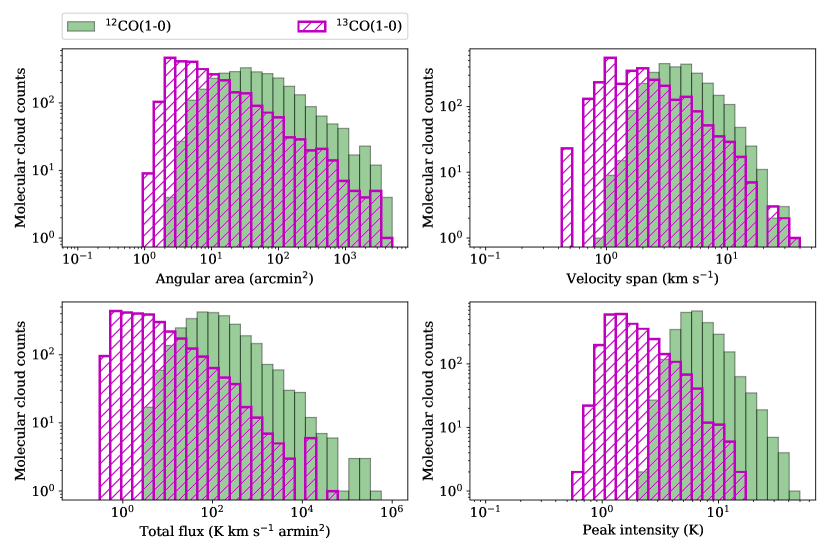
Figure 7: The number distributions of the angular sizes, velocity spans, the total fluxes and the peak intensities of ¹³CO(1-0) and ¹²CO(1-0) line emission for the 2,851 ¹³CO-detects. The green histgrams represent parameters of the ¹²CO line emission. The magenta ones are the parameters of the ¹³CO line emission.

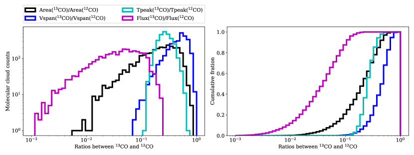
Figure 8: The counts distributions (left panel) and cumulative fractions (right panel) of the ratios between the parameters of ¹³CO structures and that of ¹²CO line emission for the 2,851 ¹³CO-detects, these parameter ratios include their angular sizes (black), velocity spans (blue), the peak intensities (cyan) and the integrated fluxes (magenta).

4.2 ¹²CO and ¹³CO lines emission in ¹²CO molecular clouds having ¹³CO structures

To systematically analyze what properties of MCs determine the ¹³CO line emission in the ¹³CO-detects, we examine the correlation between their physical properties of ¹³CO line emission with that of the ¹²CO line emission.

4.2.1 Distribution of ¹³CO and ¹²CO emission parameters

Figure 7 presents the number distributions of angular sizes ($\mathcal{A}_{\rm{}^{12}CO}$, $\mathcal{A}_{\rm{}^{13}CO}$), velocity spans ($V_{\rm{span},^{12}CO}$, $V_{\rm{span},^{13}CO}$), the integrated fluxes ($F_{\rm{}^{12}CO}$, $F_{\rm{}^{13}CO}$), and peak intensities ($T_{\rm{peak},^{12}CO}$, $T_{\rm{peak},^{13}CO}$) of ¹²CO and ¹³CO lines emission of the 2,851 ¹³CO-detects. The quantiles at 0.05, 0.25, 0.5, 0.75, and 0.95 of these parameters for ¹³CO line emission are listed in Table 5. Those for ¹²CO line emission are listed in Table 3. We find that the values of angular areas, velocity spans, peak intensities, and the integrated fluxes of ¹³CO structures in the MCs are systematically smaller than that of their ¹²CO line emission.

4.2.2 Ratios between ¹³CO and ¹²CO emission parameters

Since only a portion molecular gas components in a ¹²CO cloud have ¹³CO emission, what are the specific fractions of ¹³CO gas in these ¹²CO MCs? Figure 8 presents the distributions of the ratios between the ¹³CO emission parameters and ¹²CO emission parameters in the each ¹²CO cloud with ¹³CO structures. The quantiles at 0.05, 0.25, 0.5, 0.75, and 0.95 of these ratio values are listed in Table 5. We find that the median and mean values of $\mathcal{A}_{\rm{}^{13}CO}$/$\mathcal{A}_{\rm{}^{12}CO}$ and $T_{\rm{peak},^{13}CO}$/$T_{\rm{peak},^{12}CO}$ are close to $\sim$ 0.25. In addition, the 95$\%$ of the ¹³CO-detects have the $\mathcal{A}_{\rm{}^{13}CO}$/$\mathcal{A}_{\rm{}^{12}CO}$ with values less than 0.53 and the $T_{\rm{peak},^{13}CO}$/$T_{\rm{peak},^{12}CO}$ with values less than 0.44. For the $V_{\rm{span},^{13}CO}$/$V_{\rm{span},^{12}CO}$ in the ¹³CO-detects, their median and mean values are about 0.5 and 95$\%$ of them are less than 0.76. The median and mean values of $F_{\rm{}^{13}CO}$/$F_{\rm{}^{12}CO}$, are 0.04 and 0.05, respectively. Moreover, the $F_{\rm{}^{13}CO}$/$F_{\rm{}^{12}CO}$ for the 95$\%$ of ¹³CO-detects is not larger than 0.13. That implies the fractions of ¹³CO gas in the ¹²CO molecular clouds are typically less than 13$\%$. Considering the ¹²CO lines are more optically thick, this value should be much lower.

Table 5: The physical parameters ¹³CO emission and the ratios between the parameters of the ¹³CO and ¹²CO emission.

Types	Quantile	Angular area	Vspan	Peak Intensity	Flux
		(arcmin2)	(km s-1)	(K)	(K km s-1 arcmin2)
	0.05	2.0	0.66	1.0	0.6
	0.25	3.25	1.16	1.3	1.2
13CO emission	0.5	6.25	1.66	1.6	3.1
	0.75	16.5	2.66	2.3	10.7
	0.95	120.0	6.31	4.7	121.9
	Mean	58.4	2.37	2.1	82.0
	0.05	0.04	0.20	0.17	0.006
	0.25	0.12	0.36	0.22	0.02
13CO/12CO	0.5	0.22	0.50	0.27	0.04
	0.75	0.35	0.61	0.33	0.07
	0.95	0.53	0.76	0.44	0.13
	Mean	0.25	0.48	0.28	0.05

Note. — The quantiles at 0.05, 0.25, 0.5, 0.75 and 0.95 for each parameter in its sequential data and its mean value.

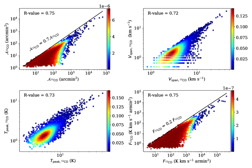
Figure 9: The correlations of angular sizes, velocity spans, peak intensities, and integrated fluxes of ¹²CO(1-0) emission between that of ¹³CO(1-0) line emission. Each dot represents a ¹²CO cloud with ¹³CO structures. The ¹²CO emission parameters of a ¹²CO cloud represent the global physical parameters of a ¹²CO clouds. The ¹³CO emission parameters are derived from all the ¹³CO structures inside a single ¹²CO cloud. The black lines represent the upper limits ($\mathcal{A}_{\rm{}^{13}CO}$ vs $\mathcal{A}_{\rm{}^{12}CO}$, $F_{\rm{}^{13}CO}$ vs $F_{\rm{}^{12}CO}$). The colors on the points represent the distribution of the probability density function of the ¹³CO-detects counts (2D-PDF), which are calculated utilizing the Kernel-density estimation through Gaussian kernels in the PYTHON package scipy.stats.gaussian_kde.

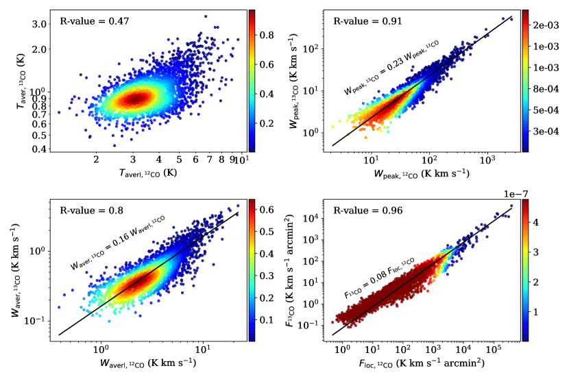
Figure 10: The correlations between the averaged line intensities ($T_{\rm{averl},^{12}CO}$ vs $T_{\rm{aver},^{13}CO}$), peak ($W_{\rm{peak},^{12}CO}$ vs $W_{\rm{peak},^{13}CO}$) and averaged ($W_{\rm{averl},^{12}CO}$ vs $W_{\rm{aver},^{13}CO}$) velocity-integrated intensities, and the integrated fluxes ($F_{\rm loc,^{12}CO}$ vs $F_{\rm{}^{13}CO}$) of ¹²CO and ¹³CO emission towards the same areas where both the ¹²CO and ¹³CO emissions are detected in each ¹³CO-detects. Each dot represents a single ¹²CO cloud with ¹³CO structures. The parameters of ¹²CO line emission are the physical parameters toward the ¹³CO-emitting regions within ¹²CO clouds. The ¹³CO emission parameters are derived from all the ¹³CO structures inside a single ¹²CO cloud. The black lines show the linear least-squares fits to the data. The colors on the points show the distribution of the probability density function of the ¹³CO-detects counts (2D-PDF).

4.2.3 Correlation between ¹³CO and ¹²CO emission parameters

Since the parameters of ¹³CO line emission are distributed in a certain range, how do the global properties of molecular clouds affect their ¹³CO line emission? Figure 9 presents the correlations between the parameters of ¹³CO emission and that of ¹²CO emission in each ¹³CO-detects. The spearman’s rank correlation coefficients (R-value) for these relations are estimated and the resultant R-values are noted in the Figure 9. We find the R-value (0.75) for $\mathcal{A}_{\rm{}^{12}CO}$ and $\mathcal{A}_{\rm{}^{13}CO}$ is consistent with that for $F_{\rm{}^{13}CO}$ and $F_{\rm{}^{12}CO}$, a little higher than the R-value (0.73) for $T_{\rm{peak},^{13}CO}$ and $T_{\rm{peak},^{12}CO}$ and the value of 0.72 for the $V_{\rm{span},^{12}CO}$ and $V_{\rm{span},^{13}CO}$. That implies there are roughly positive correlations between them, but they still present a little dispersed.

There are sharp upper limits for the ratios of $\mathcal{A}_{\rm{}^{13}CO}$/$\mathcal{A}_{\rm{}^{12}CO}$, and $F_{\rm{}^{13}CO}$/$F_{\rm{}^{12}CO}$ independent of the angular areas and CO integrated fluxes in wide ranges. As shown in Figure 9, we outline their upper limits with slopes of 0.7 and 0.2, respectively. That indicates the area of ¹³CO emission in a molecular cloud generally does not exceed the 70$\%$ of the ¹²CO emission area, independent of the ¹²CO emission area. For the integrated fluxes, the ¹³CO emission fluxes are usually less than 20$\%$ of the ¹²CO emission fluxes.

Overall, the global physical parameters of molecular clouds, such as the angular areas and integrated fluxes of ¹²CO emission, show roughly positive correlations and provide upper limits for that of ¹³CO emission. Whereas they cannot critically determine the ¹³CO emission.

Since the correlation between the global physical properties of each ¹²CO cloud and that of its interior ¹³CO structures exhibits a bit scattered, we further focus on the local areas having both ¹²CO and ¹³CO line emissions in each ¹²CO cloud with ¹³CO structures. Figure 10 presents the correlations between the parameters of ¹²CO and ¹³CO emission towards the same areas where both the ¹²CO and ¹³CO emissions are detected in each ¹³CO-detects. The $T_{\rm{averl},^{12}CO}$ is calculated by averaging the ¹²CO line intensities within the ¹³CO emission region. The $T_{\rm{aver},^{13}CO}$ is the mean value of the ¹³CO spectra intensities. The $W_{\rm{aver},^{13}CO}$ and $W_{\rm{averl},^{12}CO}$ are the averaged values of the velocity-integrated intensities of ¹³CO line and that of ¹²CO line in the ¹³CO emission region, respectively. The $W_{\rm{peak},^{13}CO}$ and $W_{\rm{peak},^{12}CO}$ are the peak values of the velocity-integrated intensity of ¹³CO lines and that of ¹²CO lines at the same positions, respectively. The $F_{\rm{}^{13}CO}$ and $F_{\rm loc,^{12}CO}$ represent the integrated fluxes of ¹³CO line emission and that of ¹²CO emission in the ¹³CO emission area, respectively. We calculate their spearman’s rank correlation coefficients (R-value) and the resultant R-values are noted in Figure 10. Based on these relations between $W_{\rm{aver},^{13}CO}$ and $W_{\rm{averl},^{12}CO}$ (R-value = 0.8), $W_{\rm peak,^{13}CO}$ and $W_{\rm peak,^{12}CO}$ (R-value = 0.91), and $F_{\rm{}^{13}CO}$ and $F_{\rm loc,^{12}CO}$ (R-value = 0.96), their correlations are more and more tightly. That indicates the properties of ¹²CO line emission in the area where both ¹²CO and ¹³CO are detected, its velocity-integrated intensity ($W_{\rm{}^{12}CO}$) in this area, is a more direct link for that of ¹³CO line emission.

Furthermore, we also implement the linear least-squares to these linear relations and the fitted slopes are noted in Figure 10. These relations indicate that the ¹³CO fluxes linearly increase as the ¹²CO fluxes incrases in the region, where the $W_{\rm{}^{12}CO}$ is larger than a value of $\sim$ 1 K km s^-1, which is close to the sensitivities of MWISP data.

4.2.4 The counts of ¹³CO molecular structures in a single ¹²CO molecular cloud

The boundary of a molecular cloud is defined by its ¹²CO(1-0) line emission, its internal ¹³CO molecular structures can present several individual structures, as shown in Figure C10. The counts of ¹³CO molecular structures in a single ¹²CO cloud can provide essential clues to the development of dense gas content and the internal sub-structures of molecular clouds. We statistic the number of separate ¹³CO molecular structures in each ¹³CO-detects. Owing to that the molecular cloud distance may affect the spatial physical resolution of ¹³CO molecular structures, we divide the 2,851 ¹³CO-detects into the near and far groups, as introduced in Section 4.1. Figure 11 presents the distributions of ¹³CO molecular structure counts in a single ¹²CO cloud for the ¹³CO-detects in near and far groups, respectively. We find that the ¹³CO-detects with one ¹³CO structure are dominant and take a percentage of about 60$\%$. Then the molecular clouds having two ¹³CO molecular structures occupied about 15$\%$ of the ¹³CO-detects. The rest $\sim$ 20$\%$ of ¹³CO-detects have more than two ¹³CO structures, the ¹³CO structure counts in a single ¹²CO cloud can be up to $\sim$ 600. It should be noted that the number fraction of ¹²CO clouds with one ¹³CO velocity structure varies about 10$\%$ for that in the near and far groups, as well as the fraction of ¹²CO clouds with multiple ¹³CO structures.

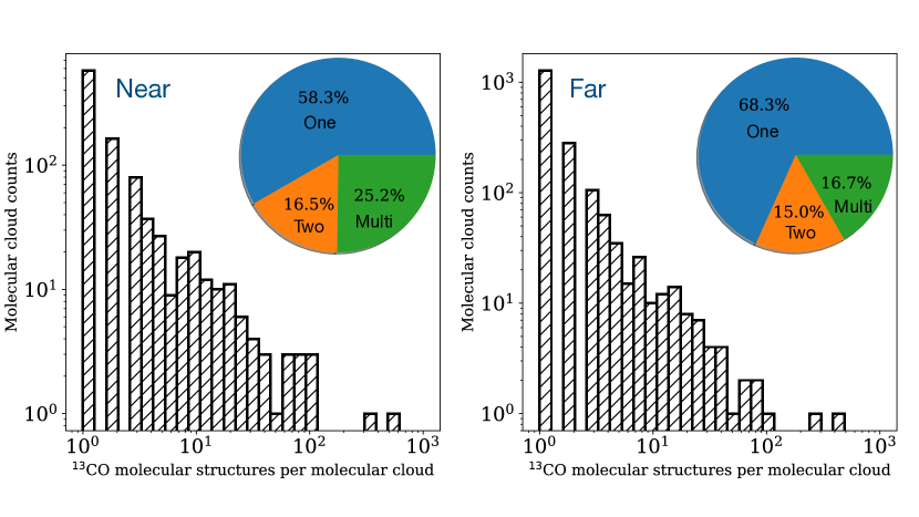
Figure 11: The distribution of the ¹³CO structure counts in a single ¹²CO cloud for the ¹³CO-detects in the near (left panel) and far (right panel) groups, respectively. In the right-up corner of each panel, the pie chart illustrates the percentages of ¹²CO clouds in this sample with one ¹³CO structure, two ¹³CO structures, and multiple (more than two) ¹³CO structures, respectively.

Table 6: The number detection rates and the total flux ratios in the total molecular clouds, nonfilaments, and filaments.

Types	All	Nonfilament	filament
Number detection rate	15.7$\%$	14.0$\%$	56.5$\%$
Flux ratio	6.3$\%$	2.9$\%$	6.7$\%$

Note. — The number detection rate is the number of extracted ¹³CO-detects divided by the number of molecular clouds in the total samples, nonfilaments and filaments, respectively. The flux ratio is the total integrated fluxes of ¹³CO line emission divided by that of ¹²CO line emission for the total molecular clouds, nonfilaments and filaments, respectively.

4.3 Linking the internal ¹³CO gas structures to the morphologies of ¹²CO clouds

4.3.1 The ¹³CO structures detection rates and morphologies

In paper I (Yuan et al., 2021), we took the morphological classification for the total 18,190 molecular clouds, which were classified as unresolved, non-filaments (11,680), and filaments (2,062). Among the 2,851 ¹³CO-detects, 1,641 ¹²CO molecular clouds belong to nonfilaments and 1,166 clouds are classified as filaments. We find that the number detection rate of ¹³CO structures is 15.7$\%$(2851/18190) in the whole ¹²CO molecular clouds, 14$\%$ (1641/11680) in the ¹²CO clouds classified as nonfilaments, and 56.5$\%$ (1166/2062) in the ¹²CO clouds classified as filaments. For the ratio of the total integrated fluxes of ¹³CO line emission to that of ¹²CO line emission, the value is 6.3$\%$ for the total molecular clouds, 2.9$\%$ for the nonfilaments, and 6.7$\%$ for the filaments. Those values are listed in Table 6. Thus, compared with nonfilaments, the filaments tend to have higher density gas structures, which are traced by ¹³CO lines.

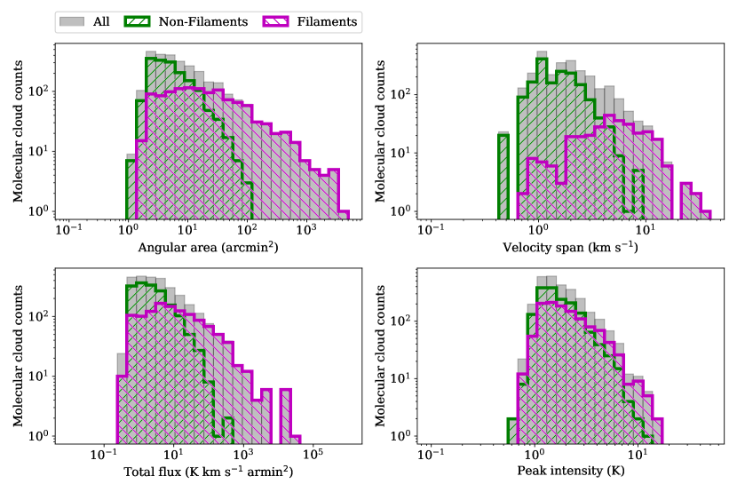
Figure 12: The number distributions of angular sizes, velocity spans, the total fluxes and the peak intensities of ¹³CO(1-0) line emission for the ¹³CO-detects classified as filaments and nonfilaments.

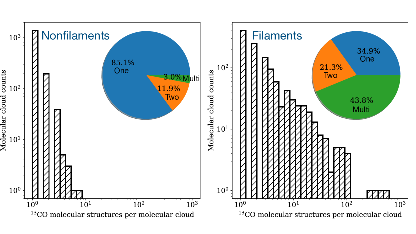
Figure 13: The distribution of the ¹³CO molecular structure counts in a single ¹²CO cloud for the ¹³CO-detects classified as nonfilaments (left panel) and filaments (right panel) groups, respectively. In the right-up corner of each panel, the pie chart illustrates the percentages of MCs in this sample with one ¹³CO molecular structure, two ¹³CO molecular structures, multiple (larger than two) ¹³CO molecular structures, respectively.

4.3.2 The ¹³CO structures parameters and morphologies

Furthermore, we focus on the properties of the ¹³CO molecular gas structures in the filaments and nonfilaments of the 2,851 ¹³CO-detects. Figure 12 compares the ¹³CO structures parameters of these filaments and nonfilaments. We find that the angular areas ($\mathcal{A}_{\rm{}^{13}CO}$), velocity spans ($V_{\rm{span},^{13}CO}$) and integrated fluxes ($F_{\rm{}^{13}CO}$) of ¹³CO structures in these filaments tend to be larger than that in these nonfilaments. While the number distributions of their peak intensities are similar. We find that filaments not only tend to have ¹³CO gas structures, but also their internal ¹³CO structures have larger angular sizes, velocity span, and integrated fluxes. That indicates the ¹²CO cloud classified as filaments gather more high-density gas structures in the local areas where both ¹²CO and ¹³CO emissions are detected.

We also link the ¹³CO molecular structure counts in a single ¹²CO cloud to its morphology. Figure 13 illustrates the distribution of ¹³CO molecular structure counts within one ¹²CO cloud for the ¹³CO-detects classified as filaments and nonfilaments. We find that about 85$\%$ of these nonfilaments have one ¹³CO molecular structure and only 3$\%$ of nonfilaments have more than two ¹³CO molecular structures. While for these filaments, those with one ¹³CO molecular structure only occupy about 35$\%$, and those having more than two ¹³CO molecular structures take about 44$\%$. Moreover, only filaments could harbor more than ten ¹³CO structures. That indicates the filament tend to have more separate ¹³CO molecular structures in its interior. That implies the development of dense gas content in filaments is separate and inhomogenous.

5 Discussion

5.1 Comparison with previous works

In the Milky Way, Torii et al. (2019) used the CO $J=1-0$ data from the FUGIN project and found that the ratio of the integrated intensities of ¹³CO and ¹²CO lines (W(¹³CO)/W(¹²CO)) along the Galactical longitude l = 10^∘ – 50^∘ were distributed in a range of 1$\%$ – 10$\%$. While the W(¹³CO)/W(¹²CO) in the star-forming cloud Orion B can achieve about 15$\%$ (Gratier et al., 2021). Roman-Duval et al. (2016) investigated the Galactic distribution of molecular gas components traced by ¹²CO and ¹³CO lines along the Galactic radius. The values of W(¹³CO)/W(¹²CO) have an approximately constant value of 20$\%$ out to the galactic radius of 6.5 kpc, decrease to $\sim$ 8$\%$ – 10$\%$ in the solar neighborhood and about 5$\%$ – 10$\%$ out to the radius of 14 kpc.

In the nearby galaxies, Cormier et al. (2018) carried out the CO observations for nine nearby spiral galaxies using IRAM 30-m telescope, which has a spatial resolution of $\sim$ 1.5 kpc, the resultant W(¹³CO)/W(¹²CO) ratio has a median value of $\sim$ 9$\%$ and varies by a factor of 2. For the five nearby star-forming galaxies, Gallagher et al. (2018) combined the IRAM ¹²CO(1-0) maps and ALMA observations of ¹³CO(1-0) lines and presented the distribution of the W(¹³CO)/W(¹²CO) along the radius, which have a mean value of 8.8$\%$ with a radius less than 1 kpc and 3.9$\%$ in a radius larger than 1 kpc. Furthermore, Méndez-Hernández et al. (2020) presented the ALMA observations towards 27 low-redshift (0.02 $<z<$ 0.2) star-forming galaxies, their averaged value of W(¹³CO)/W(¹²CO) is 5.6$\pm$1$\%$ and varies by a factor of 2.

Figure 14 compares the above literature results with our results. Overall, the W(¹³CO)/W(¹²CO) depends on not only the molecular cloud conditions but also their positions in the galaxy. Moreover, the W(¹³CO)/W(¹²CO) in the local molecular clouds with active star formation rates is higher.

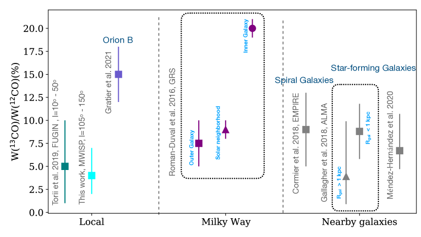
Figure 14: Comparisons among the integrated intensity ratios between ¹³CO and ¹²CO lines (W(¹³CO)/W(¹²CO)). The colored points show the average or median values of W(¹³CO)/W(¹²CO). The error bars on the individual points reflect the distributions for the ratios. From left to right, we present the literature results of W(¹³CO)/W(¹²CO) in the local regions of Milky Way and in the nearby galaxies, respectively. The W(¹³CO)/W(¹³CO), which is presented in Figure 12 of Torii et al. (2019), is calculated through the total velocity-integrated intensities of ¹³CO emission in a Galactic longitude of 1 degree divided by that of ¹²CO emission in the same bin. The presented values of this work is the ratio of the total integrated intensities of ¹³CO emission to that of ¹²CO emission in each molecular cloud. The W(¹³CO)/W(¹³CO) for the Orion B is the mean integrated intensity of ¹³CO emission divided by that of ¹²CO emission, whose values are listed in Table 2 of Gratier et al. (2021). The values of W(¹²CO) and W(¹²CO) in Roman-Duval et al. (2016); Cormier et al. (2018); Gallagher et al. (2018); Méndez-Hernández et al. (2020) are corresponds to their total luminosities in a Galactocentric radius bin, divided by the surface areas covered by the surveys in that bin, further projected onto the Galactic disk.

5.2 Implications of molecular clouds formation and evolution

The questions of how molecular clouds form and what mechanisms determine their physical properties still remain open. Several mechanisms have been invoked to explain the gathering mass of molecular clouds. The agglomeration of smaller clouds (Oort, 1954; Field & Saslaw, 1965; Kwan & Valdes, 1983; Tomisaka, 1984), the turbulence flows in the diffuse ISM (Vazquez-Semadeni et al., 1995; Passot et al., 1995; Ballesteros-Paredes et al., 1999a), and the large-scale gravitational instability of the Galactic disk (Lin & Shu, 1964; Roberts, 1969; Tasker & Tan, 2009).

From our observations of 18,190 molecular clouds using ¹²CO and ¹³CO lines. In terms of their morphologies, i.e., nonfilaments and filaments, filaments tend to have larger spatial scales. Whereas their averaged H₂ column densities do not vary significantly (Yuan et al., 2021). Furthermore, we find that ¹³CO gas emission determined by the its H₂ column density is primarily detected in the filaments. That indicates the filament gathers more mass on a global scale and meanwhile has local density enhancements where both ¹²CO and ¹³CO emissions are detected. In addition, the filament also tends to have more than one individual structure traced by ¹³CO lines in its interior. That implies the development of dense gas content in filaments is separate and inhomogenous. The formation of filament often arises from the shock compression in the ISM (Arzoumanian et al., 2018; Abe et al., 2021; Arzoumanian et al., 2022). The shock compression may be caused by supersonic turbulence in the molecular clouds (Padoan & Nordlund, 1999; Pudritz & Kevlahan, 2013; Matsumoto et al., 2015), cloud collisions (Inoue & Fukui, 2013; Inoue et al., 2018; Tokuda et al., 2019), feedback from massive stars, and galactic spiral shock. While the supercritical filaments may be driven by the gravitational contraction/accretion (Arzoumanian et al., 2013; Gong et al., 2021; Yuan et al., 2020) and further fragment into smaller components owning to turbulence and gravitational instabilities (Hacar & Tafalla, 2011; Henshaw et al., 2016; Kainulainen et al., 2017; Lu et al., 2018; Lin et al., 2019; Yuan et al., 2019).

We try to investigate the relation between the filaments and nonfilaments. If the filaments fragment into nonfilaments due to the gravitational instability, the high-density gas fraction in nonfilaments should be comparable to that of filaments. That is unlikely owing to our observational results of nonfilaments with less dense gas. Our observed properties of filaments and nonfilaments favor that molecular clouds be explained as the density fluctuations induced by the turbulent compression in the diffuse ISM and broken up by the combination of dynamical and thermal instabilities, like the physical processes of shear, rotation, cooling, and magnetic fields (Ballesteros-Paredes et al., 1999b; Koyama & Inutsuka, 2002; Heitsch et al., 2006; Vázquez-Semadeni et al., 2006; Beuther et al., 2020). Filaments tend to be under shock compressions and nonfilaments tend to be in low-pressure environments. Meanwhile they present the different spatial scales and internal structures. In addition, we are not able to rule out the hypothesis that nonfilament collisions to form filaments to some degree.

6 Summary and conclusions

We identify the ¹³CO gas structures in the 18,190 ¹²CO molecular clouds and systematically compare the physical properties of ¹²CO clouds having ¹³CO gas structures (¹³CO-detects) and those of ¹²CO clouds without ¹³CO gas structures (Non¹³CO-detects). Furthermore, we systematically analyze the ¹³CO and ¹²CO emission parameters in the 2851 ¹³CO-detects, and link the internal ¹³CO gas structures of each ¹²CO cloud with its morphology, i.e., filament or nonfilament. The main conclusions are as follows:

1. In the whole sample of 18,190 ¹²CO molecular clouds, $\sim$ 15.7$\%$ ¹²CO clouds (2851) have the ¹³CO molecular gas structures. The total integrated fluxes of ¹²CO line emission for the ¹³CO-detects are about 93$\%$ of that for the whole sample of molecular clouds.

2. In the 2851 ¹³CO-detects, we find the ¹³CO structures’ area in a ¹²CO cloud generally does not exceed 70$\%$ of the ¹²CO emission area, independently of the ¹²CO emission area, and its interior integrated fluxes of ¹³CO emission are usually less than 20$\%$ of those of its ¹²CO emission.

3. In the 2851 ¹³CO-detects, we find a strong correlation between the velocity-integrated intensities of ¹²CO lines and those of ¹³CO lines emission in the same areas where both the ¹²CO and ¹³CO emissions are detected.

4. In the 2851 ¹³CO-detects, we find that there are $\sim$ 60$\%$ of ¹²CO clouds have one individual ¹³CO structure, about 15$\%$ of ¹²CO clouds have two separate ¹³CO structures, and the rest of them have more than two separate ¹³CO structures.

5. We link the ¹³CO gas fractions in the ¹³CO-detects with their morphologies, i.e., filaments or nonfilaments, and find that the ¹³CO line emissions are primarily detected in the ¹²CO clouds classified as filaments. In addition, a filament tends to have more than one individual ¹³CO structure in its interior.

Appendix A ¹³CO($J=$ 1-0) lines data

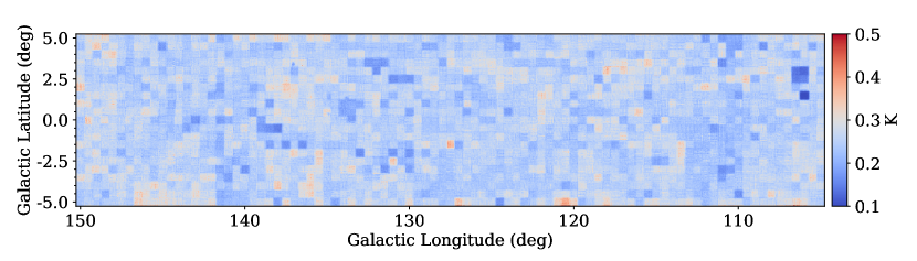
Figure A1: The distribution of the background noise RMS in the second Galactic quadrant with 104.75^∘ $<l<$ 150.25^∘ and $|b|<$ 5.25^∘.

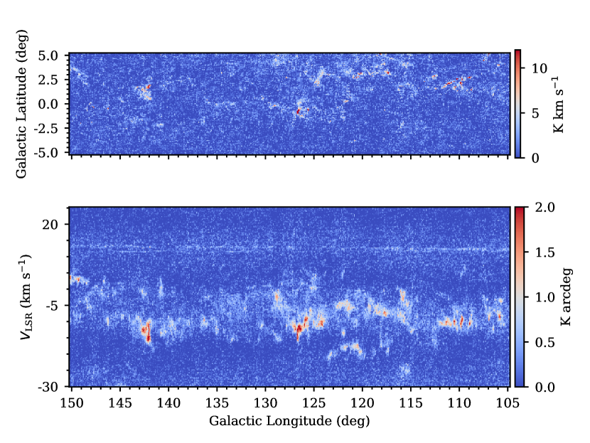
Figure A2: Top Panel: the velocity-integrated intensity map of ¹³CO(1-0) emission in the near group. This map is derived by integrating the ¹³CO emission over the velocity range between $-$30 km s^-1 and 25 km s^-1. The sensitivity for this velocity-integrated is about 0.77 K km s^-1. Bottom Panel: the latitude-integrated intensity map of ¹³CO(1-0) emission in the near group. This map is derived by integrating the ¹³CO emission over the latitude range from $-$5.25^∘ to 5.25^∘.

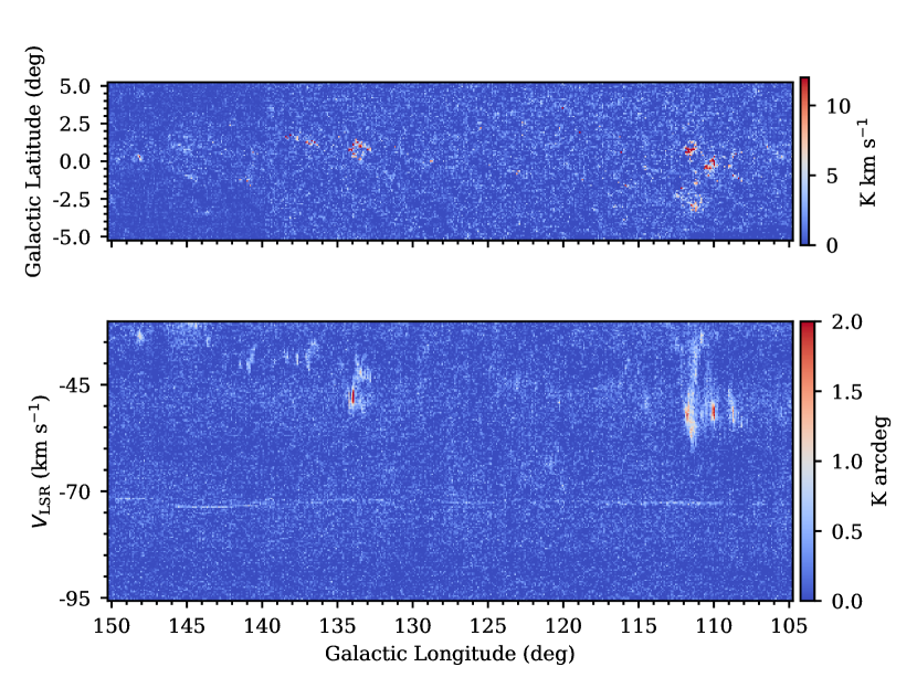
Figure A3: Top Panel: the velocity-integrated intensity map of ¹³CO(1-0) emission in the far group. This map is derived by integrating the ¹³CO emission over the velocity range between $-$95 km s^-1 and $-$30 km s^-1. The sensitivity for this velocity-integrated is about 0.83 K km s^-1. Bottom Panel: the latitude-integrated intensity map of ¹³CO(1-0) emission in the far group. This map is derived by integrating the ¹³CO emission over the latitude range from $-$5.25^∘ to 5.25^∘.

Appendix B The parameters of DBSCAN algorithm

The DBSCAN algorithm extracts the consecutive structures in the PPV space of CO lines data, based on a line intensity threshold and two parameters, i.e. $\epsilon$ and MinPts. Two parameters of $\epsilon$ and MinPts define the connectivity of structures in the PPV space. Each point within the extracted consecutive structure is called a core point. For a core point, its adjacent points contained in its neighborhood has to exceed a threshold. The parameter of MinPts determines the threshold of the number of adjacent points and the $\epsilon$ represents the radius of the neighborhood. A border point in the consecutive structure is defined as a point inside the $\epsilon$-neighborhood of a core point, but not necessarily contain the MinPts neighbors, as shown in Figure 2 of (Ester et al., 1996). In the PPV space of CO data, Yan et al. (2020) has examined all the choices of parameters and ¹²CO line intensities cutoffs to identify molecular clouds. The parameters of cutoff = 2$\sigma$, minPts = 4, $\epsilon$ = 1 are used in the DBSCAN algorithm to extract the ¹²CO molecular clouds in the ¹²CO data cube, as well as the ¹³CO molecular structures within the ¹²CO molecular cloud. The post-selection criteria are examined and utilized to avoid the noise contamination (Yan et al., 2020). These criteria for a extracted structure include: (1) the minimum voxel number is 16; (2) the peak intensity is larger than the value of cutoff + 3$\sigma$ for ¹²CO or cutoff + 2$\sigma$ for ¹³CO; (3) the angular area is large than one beam size (2$\times$2 pixels); (4) the number of velocity channels are larger than 3.

Appendix C The ¹³CO structures of the molecular cloud G139.73 extracted by three methods

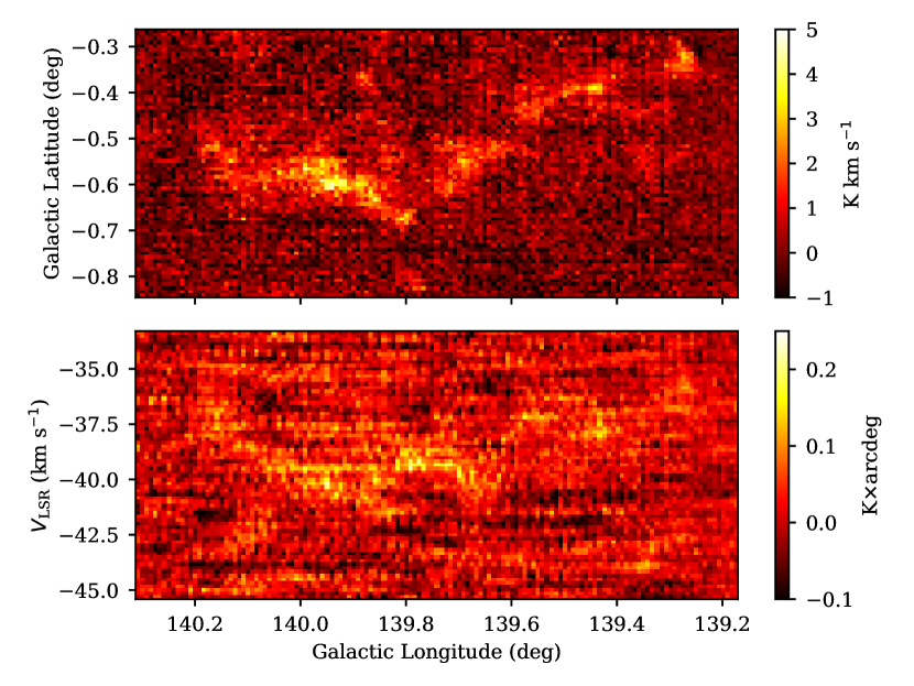
Figure C5: The velocity-integrated intensity map (upper) and latitude-integrated intensity map (lower) of ¹³CO emission for the molecular cloud G139.73, which are derivied by the raw chopped ¹³CO data cube without any clipping.

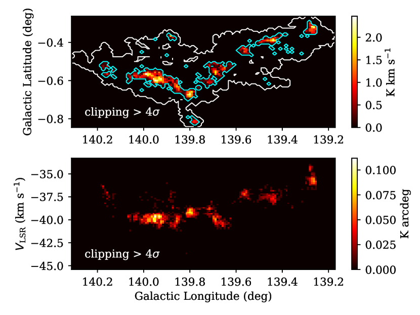
Figure C8: Same as Figure C7, but using the clipping at the cutoff level of 4$\sigma$ (1.08 K).

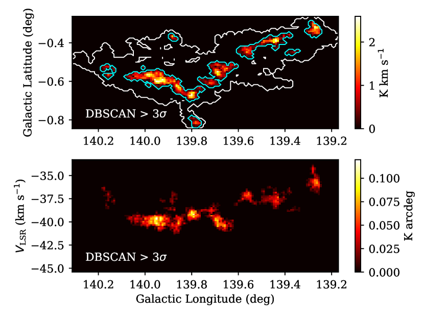
Figure C11: Same as Figure C7, but using the DBSCAN at the cutoff level of 3$\sigma$ (0.81 K).

Figure C13: Same as Figure C7, but using the moment mask at the cutoff level of 8$\sigma_{\rm sm}$ (0.4 K).

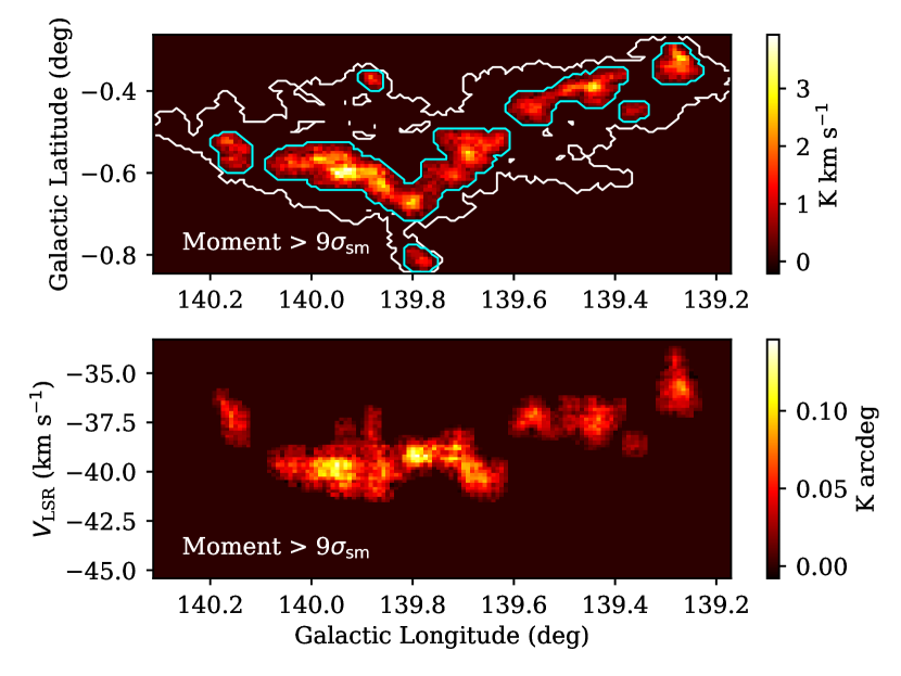
Figure C14: Same as Figure C7, but using the moment mask at the cutoff level of 9$\sigma_{\rm sm}$ (0.45 K).

Appendix D Random examples of molecular clouds with ¹³CO structures

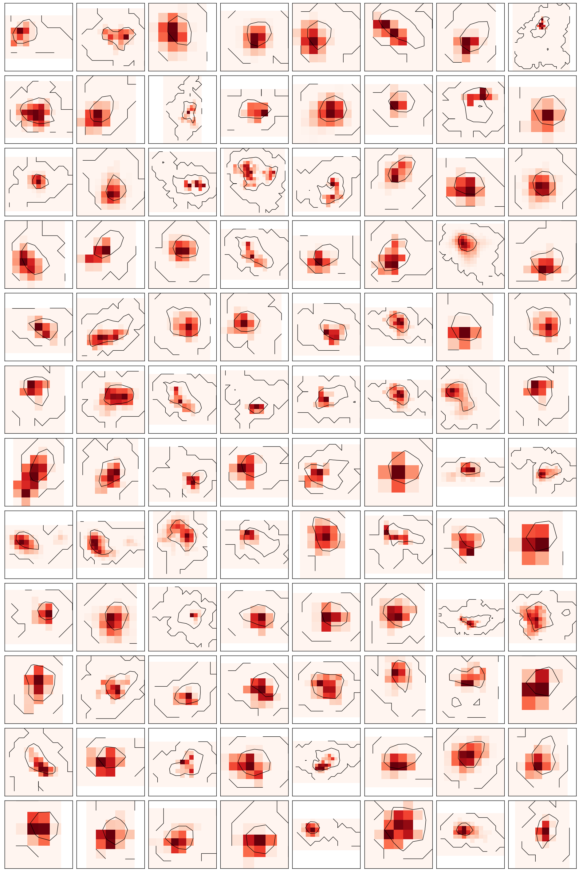
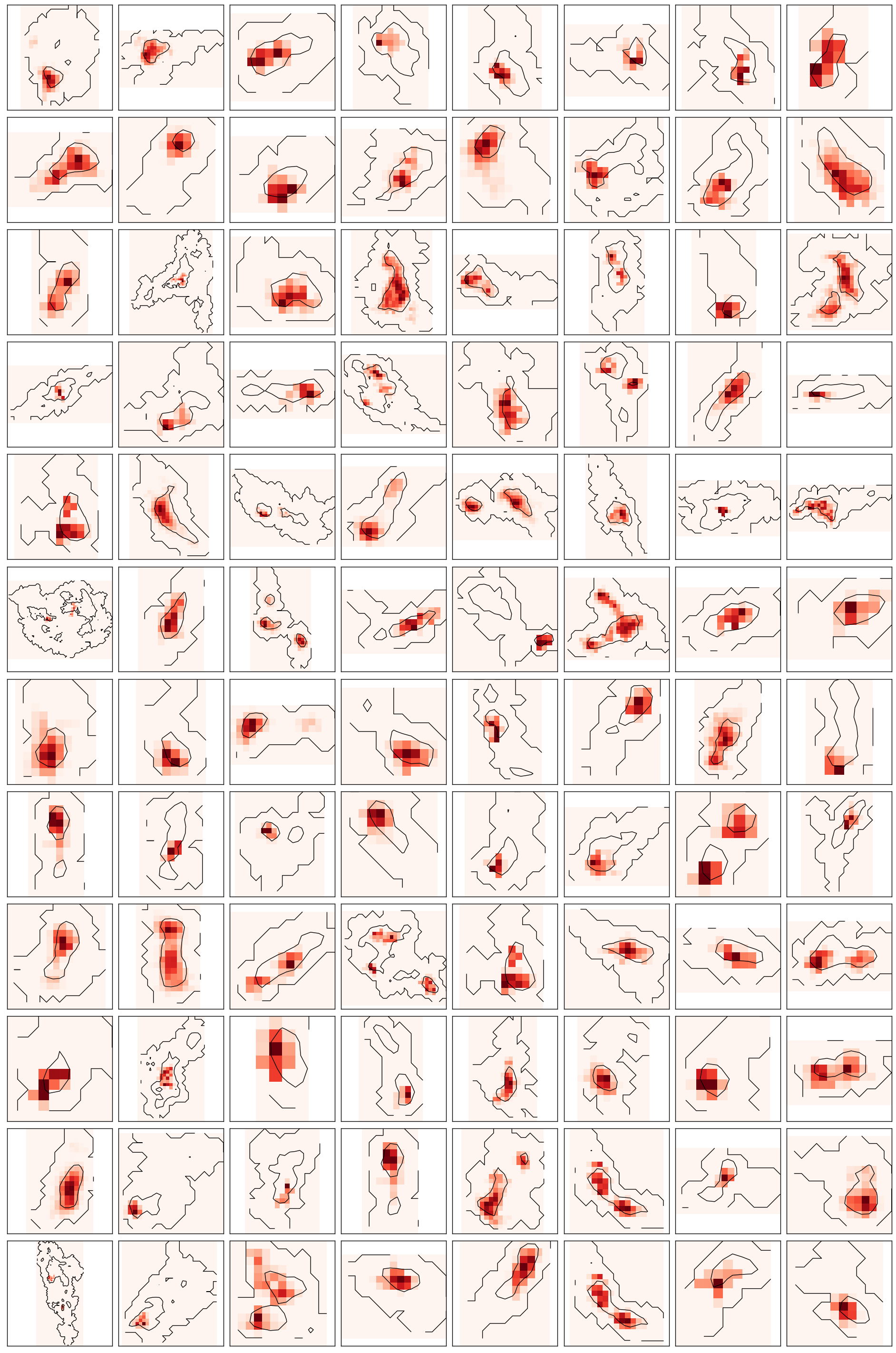
Figure D16: ¹³CO structures identified by the DBSCAN. The colormaps represent the distributions of the velocity-integrated intensities of ¹³CO line emission. The black contours indicate the boundaries and the level of 50$\%$ at the ¹²CO line velocity-integrated intensities.

Figure D17: Same as above.

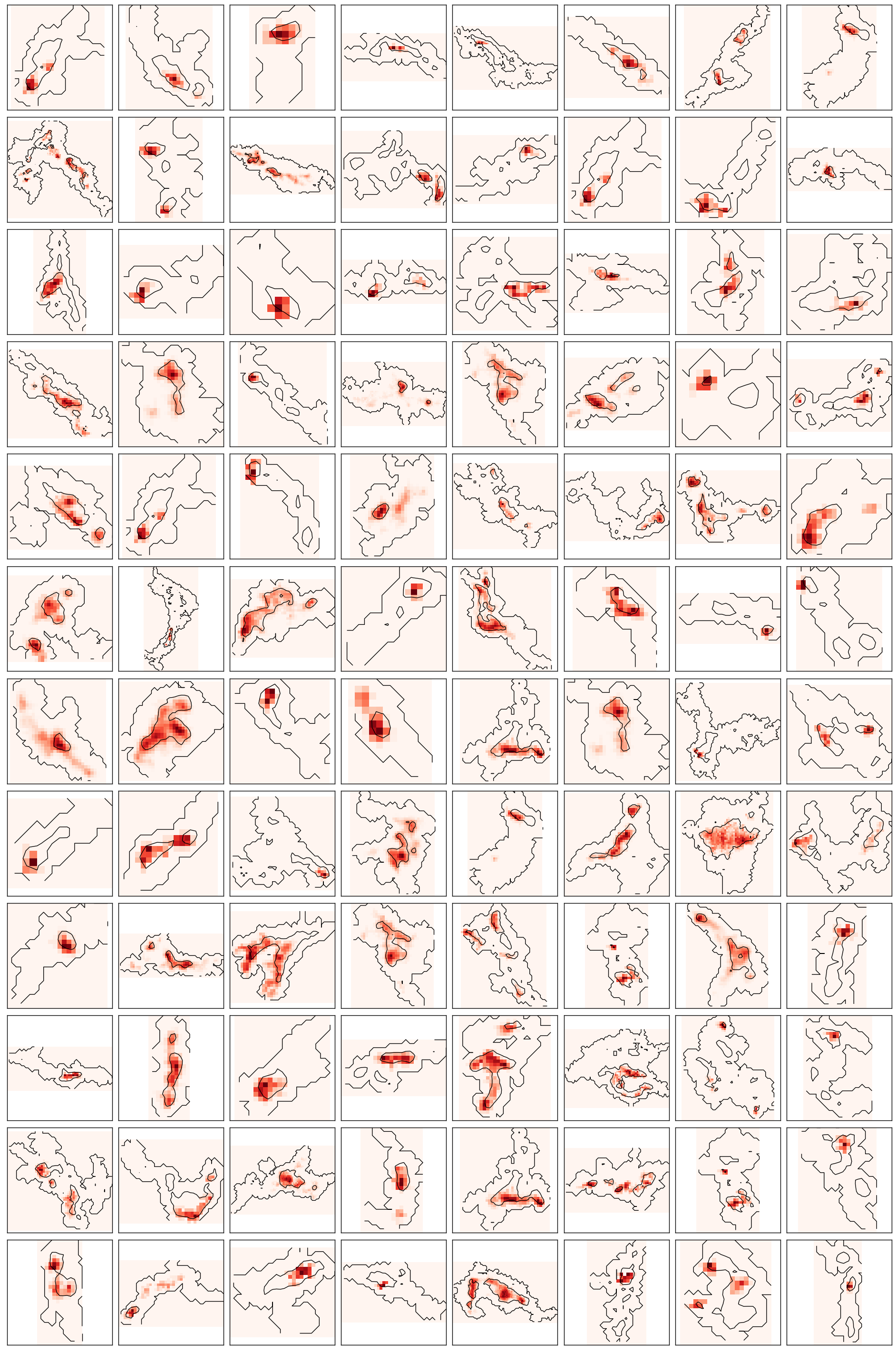
Figure D18: Same as above.

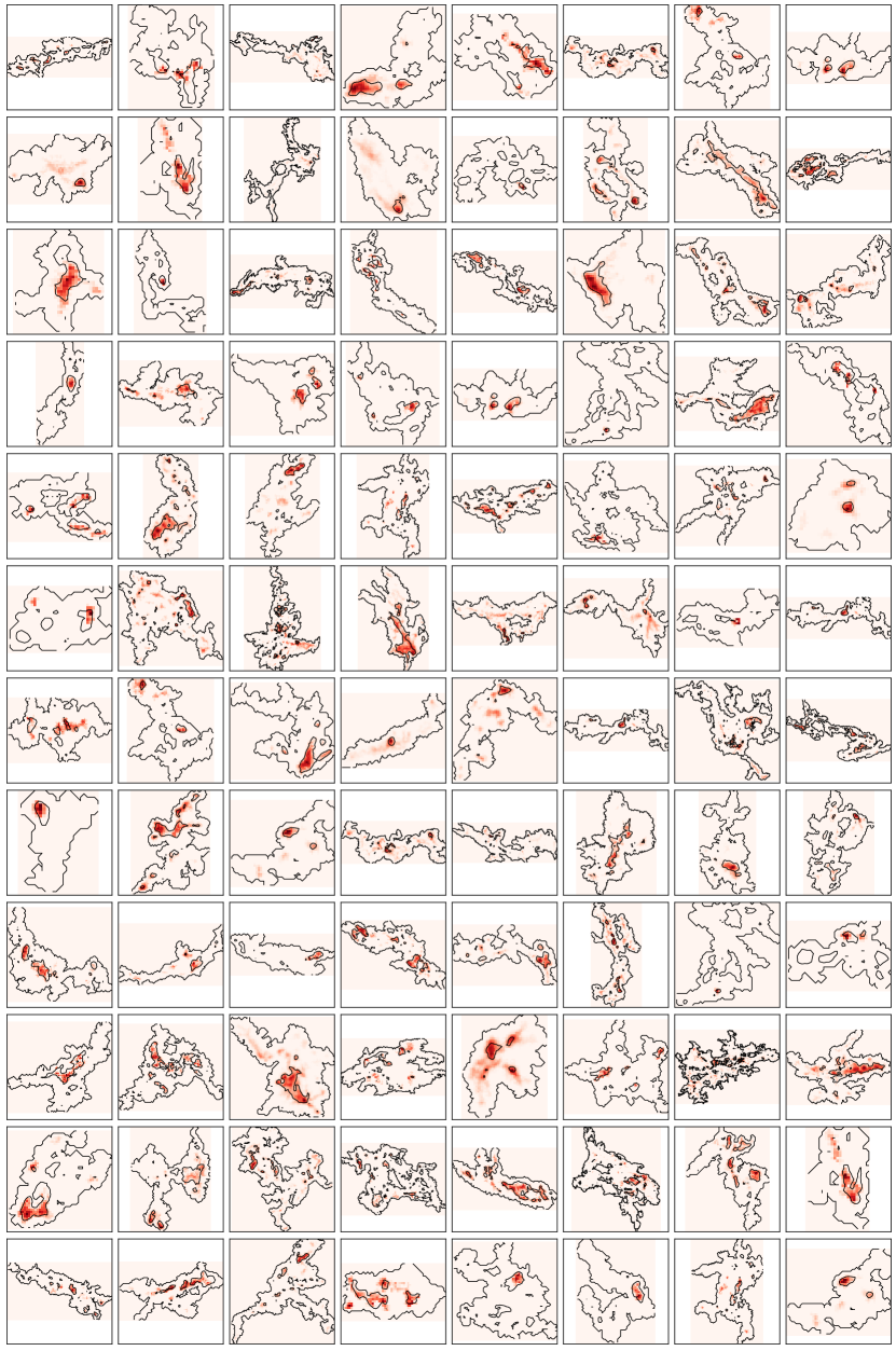
Figure D19: Same as above.

References

- Abe et al. (2021) Abe, D., Inoue, T., Inutsuka, S.-i., & Matsumoto, T. 2021, ApJ, 916, 83, doi: 10.3847/1538-4357/ac07a1
- André et al. (2014) André, P., Di Francesco, J., Ward-Thompson, D., et al. 2014, in Protostars and Planets VI, ed. H. Beuther, R. S. Klessen, C. P. Dullemond, & T. Henning, 27, doi: 10.2458/azu_uapress_9780816531240-ch002
- André et al. (2010) André, P., Men’shchikov, A., Bontemps, S., et al. 2010, A&A, 518, L102, doi: 10.1051/0004-6361/201014666
- André et al. (2016) André, P., Revéret, V., Könyves, V., et al. 2016, A&A, 592, A54, doi: 10.1051/0004-6361/201628378
- Arzoumanian et al. (2013) Arzoumanian, D., André, P., Peretto, N., & Könyves, V. 2013, A&A, 553, A119, doi: 10.1051/0004-6361/201220822
- Arzoumanian et al. (2018) Arzoumanian, D., Shimajiri, Y., Inutsuka, S.-i., Inoue, T., & Tachihara, K. 2018, PASJ, 70, 96, doi: 10.1093/pasj/psy095
- Arzoumanian et al. (2022) Arzoumanian, D., Russeil, D., Zavagno, A., et al. 2022, arXiv e-prints, arXiv:2201.04267. https://arxiv.org/abs/2201.04267
- Astropy Collaboration et al. (2013) Astropy Collaboration, Robitaille, T. P., Tollerud, E. J., et al. 2013, A&A, 558, A33, doi: 10.1051/0004-6361/201322068
- Astropy Collaboration et al. (2018) Astropy Collaboration, Price-Whelan, A. M., Sipőcz, B. M., et al. 2018, AJ, 156, 123, doi: 10.3847/1538-3881/aabc4f
- Ballesteros-Paredes et al. (1999a) Ballesteros-Paredes, J., Vázquez-Semadeni, E., & Scalo, J. 1999a, ApJ, 515, 286, doi: 10.1086/307007
- Ballesteros-Paredes et al. (1999b) —. 1999b, ApJ, 515, 286, doi: 10.1086/307007
- Beuther et al. (2020) Beuther, H., Wang, Y., Soler, J., et al. 2020, A&A, 638, A44, doi: 10.1051/0004-6361/202037950
- Bolatto et al. (2013) Bolatto, A. D., Wolfire, M., & Leroy, A. K. 2013, ARA&A, 51, 207, doi: 10.1146/annurev-astro-082812-140944
- Cormier et al. (2018) Cormier, D., Bigiel, F., Jiménez-Donaire, M. J., et al. 2018, MNRAS, 475, 3909, doi: 10.1093/mnras/sty059
- Dame (2011) Dame, T. M. 2011, arXiv e-prints, arXiv:1101.1499. https://arxiv.org/abs/1101.1499
- Dobbs & Baba (2014) Dobbs, C., & Baba, J. 2014, PASA, 31, e035, doi: 10.1017/pasa.2014.31
- Ester et al. (1996) Ester, M., Kriegel, H.-P., Sander, J., & Xu, X. 1996, in Proceedings of the Second International Conference on Knowledge Discovery and Data Mining, KDD’96 (AAAI Press), 226–231. http://dl.acm.org/citation.cfm?id=3001460.3001507
- Field & Saslaw (1965) Field, G. B., & Saslaw, W. C. 1965, ApJ, 142, 568, doi: 10.1086/148318
- Gallagher et al. (2018) Gallagher, M. J., Leroy, A. K., Bigiel, F., et al. 2018, ApJ, 858, 90, doi: 10.3847/1538-4357/aabad8
- Goldreich & Lynden-Bell (1965) Goldreich, P., & Lynden-Bell, D. 1965, MNRAS, 130, 97, doi: 10.1093/mnras/130.2.97
- Gong et al. (2021) Gong, Y., Belloche, A., Du, F. J., et al. 2021, A&A, 646, A170, doi: 10.1051/0004-6361/202039465
- Gratier et al. (2021) Gratier, P., Pety, J., Bron, E., et al. 2021, A&A, 645, A27, doi: 10.1051/0004-6361/202037871
- Hacar & Tafalla (2011) Hacar, A., & Tafalla, M. 2011, A&A, 533, A34, doi: 10.1051/0004-6361/201117039
- Heitsch et al. (2006) Heitsch, F., Slyz, A. D., Devriendt, J. E. G., Hartmann, L. W., & Burkert, A. 2006, ApJ, 648, 1052, doi: 10.1086/505931
- Henshaw et al. (2016) Henshaw, J. D., Caselli, P., Fontani, F., et al. 2016, MNRAS, 463, 146, doi: 10.1093/mnras/stw1794
- Heyer & Dame (2015) Heyer, M., & Dame, T. M. 2015, ARA&A, 53, 583, doi: 10.1146/annurev-astro-082214-122324
- Hunter (2007) Hunter, J. D. 2007, Computing in Science & Engineering, 9, 90, doi: 10.1109/MCSE.2007.55
- Inoue & Fukui (2013) Inoue, T., & Fukui, Y. 2013, ApJ, 774, L31, doi: 10.1088/2041-8205/774/2/L31
- Inoue et al. (2018) Inoue, T., Hennebelle, P., Fukui, Y., et al. 2018, PASJ, 70, S53, doi: 10.1093/pasj/psx089
- Kainulainen et al. (2017) Kainulainen, J., Stutz, A. M., Stanke, T., et al. 2017, A&A, 600, A141, doi: 10.1051/0004-6361/201628481
- Koyama & Inutsuka (2002) Koyama, H., & Inutsuka, S.-i. 2002, ApJ, 564, L97, doi: 10.1086/338978
- Kwan & Valdes (1983) Kwan, J., & Valdes, F. 1983, ApJ, 271, 604, doi: 10.1086/161227
- Lin & Shu (1964) Lin, C. C., & Shu, F. H. 1964, ApJ, 140, 646, doi: 10.1086/147955
- Lin et al. (2019) Lin, Y., Csengeri, T., Wyrowski, F., et al. 2019, A&A, 631, A72, doi: 10.1051/0004-6361/201935410
- Lu et al. (2018) Lu, X., Zhang, Q., Liu, H. B., et al. 2018, ApJ, 855, 9, doi: 10.3847/1538-4357/aaad11
- Matsumoto et al. (2015) Matsumoto, T., Dobashi, K., & Shimoikura, T. 2015, ApJ, 801, 77, doi: 10.1088/0004-637X/801/2/77
- Méndez-Hernández et al. (2020) Méndez-Hernández, H., Ibar, E., Knudsen, K. K., et al. 2020, MNRAS, 497, 2771, doi: 10.1093/mnras/staa1964
- Molinari et al. (2010) Molinari, S., Swinyard, B., Bally, J., et al. 2010, A&A, 518, L100, doi: 10.1051/0004-6361/201014659
- Neralwar et al. (2022a) Neralwar, K. R., Colombo, D., Duarte-Cabral, A., et al. 2022a, arXiv e-prints, arXiv:2203.02504. https://arxiv.org/abs/2203.02504
- Neralwar et al. (2022b) —. 2022b, arXiv e-prints, arXiv:2205.02253. https://arxiv.org/abs/2205.02253
- Oort (1954) Oort, J. H. 1954, Bull. Astron. Inst. Netherlands, 12, 177
- Padoan & Nordlund (1999) Padoan, P., & Nordlund, Å. 1999, ApJ, 526, 279, doi: 10.1086/307956
- Passot et al. (1995) Passot, T., Vazquez-Semadeni, E., & Pouquet, A. 1995, ApJ, 455, 536, doi: 10.1086/176603
- Peretto et al. (2022) Peretto, N., Adam, R., Ade, P., et al. 2022, in European Physical Journal Web of Conferences, Vol. 257, European Physical Journal Web of Conferences, 00037, doi: 10.1051/epjconf/202225700037
- Pudritz & Kevlahan (2013) Pudritz, R. E., & Kevlahan, N. K. R. 2013, Philosophical Transactions of the Royal Society of London Series A, 371, 20120248, doi: 10.1098/rsta.2012.0248
- Reid et al. (2016) Reid, M. J., Dame, T. M., Menten, K. M., & Brunthaler, A. 2016, ApJ, 823, 77, doi: 10.3847/0004-637X/823/2/77
- Roberts (1969) Roberts, W. W. 1969, ApJ, 158, 123, doi: 10.1086/150177
- Roman-Duval et al. (2016) Roman-Duval, J., Heyer, M., Brunt, C. M., et al. 2016, ApJ, 818, 144, doi: 10.3847/0004-637X/818/2/144
- Su et al. (2019) Su, Y., Yang, J., Zhang, S., et al. 2019, ApJS, 240, 9, doi: 10.3847/1538-4365/aaf1c8
- Tasker & Tan (2009) Tasker, E. J., & Tan, J. C. 2009, ApJ, 700, 358, doi: 10.1088/0004-637X/700/1/358
- Tokuda et al. (2019) Tokuda, K., Fukui, Y., Harada, R., et al. 2019, ApJ, 886, 15, doi: 10.3847/1538-4357/ab48ff
- Tomisaka (1984) Tomisaka, K. 1984, PASJ, 36, 457
- Torii et al. (2019) Torii, K., Fujita, S., Nishimura, A., et al. 2019, PASJ, 71, S2, doi: 10.1093/pasj/psz033
- Vazquez-Semadeni et al. (1995) Vazquez-Semadeni, E., Passot, T., & Pouquet, A. 1995, ApJ, 441, 702, doi: 10.1086/175393
- Vázquez-Semadeni et al. (2006) Vázquez-Semadeni, E., Ryu, D., Passot, T., González, R. F., & Gazol, A. 2006, ApJ, 643, 245, doi: 10.1086/502710
- Wilson et al. (1970) Wilson, R. W., Jefferts, K. B., & Penzias, A. A. 1970, ApJ, 161, L43, doi: 10.1086/180567
- Yan et al. (2020) Yan, Q.-Z., Yang, J., Su, Y., Sun, Y., & Wang, C. 2020, ApJ, 898, 80, doi: 10.3847/1538-4357/ab9f9c
- Yan et al. (2021) Yan, Q.-Z., Yang, J., Sun, Y., et al. 2021, A&A, 645, A129, doi: 10.1051/0004-6361/202039768
- Yuan et al. (2022) Yuan, L., Yang, J., Du, F., & Su, Y. 2022, The 12CO and 13CO lines data of 18,190 molecular clouds from the MWISP CO survey, V1, Science Data Bank, doi: 10.57760/sciencedb.j00001.00427
- Yuan et al. (2019) Yuan, L., Zhu, M., Liu, T., et al. 2019, MNRAS, 487, 1315, doi: 10.1093/mnras/stz1266
- Yuan et al. (2020) Yuan, L., Li, G.-X., Zhu, M., et al. 2020, A&A, 637, A67, doi: 10.1051/0004-6361/201936625
- Yuan et al. (2021) Yuan, L., Yang, J., Du, F., et al. 2021, ApJS, 257, 51, doi: 10.3847/1538-4365/ac242a