Informable Multi-Objective and Multi-Directional RRT^∗
System for Robot Path Planning

Abstract

Multi-objective or multi-destination path planning is crucial for mobile robotics applications such as mobility as a service, robotics inspection, and electric vehicle charging for long trips. This work proposes an anytime iterative system to concurrently solve the multi-objective path planning problem and determine the visiting order of destinations. The system is comprised of an anytime informable multi-objective and multi-directional RRT^∗ algorithm to form a simple connected graph, and a proposed solver that consists of an enhanced cheapest insertion algorithm and a genetic algorithm to solve the relaxed traveling salesman problem in polynomial time. Moreover, a list of waypoints is often provided for robotics inspection and vehicle routing so that the robot can preferentially visit certain equipment or areas of interest. We show that the proposed system can inherently incorporate such knowledge, and can navigate through challenging topology. The proposed anytime system is evaluated on large and complex graphs built for real-world driving applications. All implementations are coded in multi-threaded C++ and are available at: https://github.com/UMich-BipedLab/IMOMD-RRTStar.

1 Introduction and Contributions

Multi-objective or multi-destination path planning is a key enabler of applications such as data collection [1, 2, 3], traditional Traveling Salesman Problem (TSP) [4, 5], and electric vehicle charging for long trips. More recently, autonomous “Mobility as a Service” (e.g., autonomous shuttles or other local transport between user-selected points) has become another important application of multi-objective planning such as car-pooling [6, 7, 8, 9] Therefore, being able to efficiently find paths connecting multiple destinations and to determine the visiting order of the destinations (essentially, a relaxed TSP) is critical for modern navigation systems deployed by autonomous vehicles and robots. This paper seeks to solve these two problems by developing a system composed of a sampling-based anytime path planning algorithm and a relaxed-TSP solver.

Another application of multi-objective path planning is robotics inspection, where a list of inspection waypoints is often provided so that the robot can preferentially examine certain equipment or areas of interest or avoid certain areas in a factory, for example. The pre-defined waypoints can be considered as prior knowledge for the overall inspection path the robot needs to construct for task completion. We show that the proposed system can inherently incorporate such knowledge.

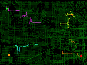
(a)

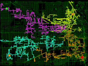
(b)

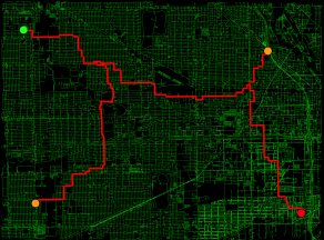
(c)

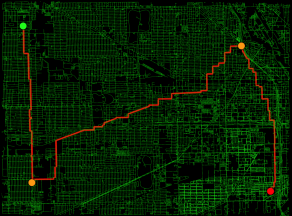
(d)

Figure 1: Illustration of the proposed informable multi-objective and multi-directional RRT^∗ ($\text{IMOMD-RRT}^{*}$) system evaluated on OpenStreetMap of Chicago, containing $866,089$ nodes and $1,038,414$ edges. The green, red, and orange dots are the source, target, and objectives, respectively. LABEL:sub@fig:FirstImg1 shows the initial stage of the tree expansion of each destination. LABEL:sub@fig:FirstImg2 shows the trees from each destination form a connected graph. LABEL:sub@fig:FirstImg3 shows the first path and visiting order from the $\text{IMOMD-RRT}^{*}$. Given more computation time, LABEL:sub@fig:FirstImg4 shows that $\text{IMOMD-RRT}^{*}$ returns a better path and order.

To represent multiple destinations, graphs composed of nodes and edges stand out for their sparse representations. In particular, graphs are a popular representation of topological landscape features, such as terrain contour, lane markers, or intersections [10]. Topological features do not change often; thus, they are maintainable and suitable for long-term support compared to high-definition (HD) maps. Graph-based maps such as OpenStreetMap [10] have been developed over the past two decades to describe topological features and are readily available worldwide. Therefore, we concentrate on developing the proposed informable multi-objective and multi-directional rapidly-exploring random trees (RRT^∗) system for path planning on large and complex graphs.

A multi-objective path planning system is charged with two tasks: 1) find weighted paths (i.e., paths and traversal costs), if they exist, that connect the various destinations. This operation results in an undirected and weighted graph where nodes and edges correspond to destinations and paths connecting destinations, respectively. 2) determine the visiting order of destinations that minimizes total travel cost. The second task, called relaxed TSP, differs from standard TSP in that we are allowed to (or sometimes have to) visit a node multiple times; see Sec. 2.3 for a detailed discussion. Several approaches [11, 12, 13, 14] have been developed to solve each of these tasks separately, assuming either the visiting order of the destinations is given, or a cyclic/complete graph is constructed and the weights of edges are provided. However, in real-time applications, the connectivity of the destinations and the weights of the paths between destinations (task 1) as well as the visiting order of the destinations (task 2) are often unknown. It is crucial that we are able to solve these two tasks concurrently in an anytime manner, meaning that the system can provide suboptimal but monotonically improving solutions at any time throughout the path cost minimization process.

In this paper, we seek to develop an anytime iterative system to provide paths between multiple objectives and to determine the visiting order of destinations; moreover, the system should be informable meaning it can accommodate prior knowledge of intermediate nodes, if available. The proposed system consists of two components: 1) an anytime informable multi-objective and multi-directional RRT^∗ ($\text{IMOMD-RRT}^{*}$) algorithm to form a connected weighted-undirected graph, and 2) a relaxed TSP solver that consists of an enhanced version of the cheapest insertion algorithm [15] and a genetic algorithm [16, 17, 18, 19], which together we call ECI-Gen. The proposed system is evaluated on large-complex graphs built for real-world driving applications, such as the OpenStreetMap of Chicago containing $866,089$ nodes and $1,038,414$ edges that is shown in Fig. 1.

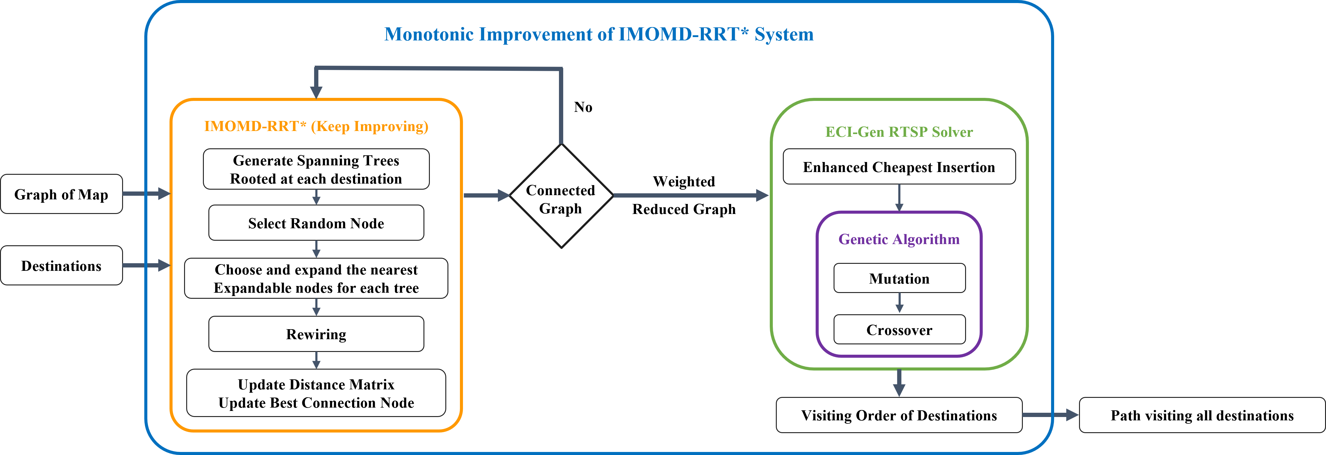
Figure 2: Illustration of the proposed $\text{IMOMD-RRT}^{*}$ system. It consists of an anytime informable multi-objective and multi-directional RRT^∗ ($\text{IMOMD-RRT}^{*}$) algorithm to construct a connected weighted-undirected graph, and a polynomial-time solver to solve the relaxed TSP. The solver consists of an enhanced version of the cheapest insertion algorithm [15] and a genetic algorithm [16, 17, 18], called ECI-Gen solver. The full system (the blue box) will continue to run to further improve the solution over time.

The overall system is shown in Fig. 2 includes the following contributions:

1. An anytime informable multi-objective and multi-directional RRT^∗ ($\text{IMOMD-RRT}^{*}$) system that functions on large-complex graphs. The anytime features means that the system quickly constructs a path on a large-scale undirected weighted graph that meets the existence constraint (the solution path must passes by all the objectives at least once), and the order constraint (with fixed starting point and end point). Therefore, the resulting weighted reduced graph containing the objectives, source, and target is connected.

2. The problem of determining the visiting order of destinations of the connected graph is a relaxed TSP (R-TSP) with fixed start and end nodes, though intermediate nodes can be (or sometimes must be) visited more than once. We introduce the ECI-Gen solver, which is based on an enhancement of the cheapest insertion algorithm [15] and a genetic algorithm [16, 17, 18, 19] to solve the R-TSP in polynomial time.

3. We show that prior knowledge (such as a reference path) for robotics inspection of a pipe or factory can be readily and inherently integrated into the $\text{IMOMD-RRT}^{*}$. In addition, providing the prior knowledge to the planner can help navigate through challenging topology.

4. We evaluate the system comprised of $\text{IMOMD-RRT}^{*}$ and the ECI-Gen solver on large-scale graphs built for real world driving applications, where the large number of intermediate destinations precludes solving the ordering by brute force. We show that the proposed IMOMD-RRT^∗ outperforms bi-directional A^∗ [20] and ANA^∗ [21] in terms of speed and memory usage in large and complex graphs. We also demonstrate by providing a reference path, the $\text{IMOMD-RRT}^{*}$ escapes from bug traps (e.g., single entry neighborhoods) in complex graphs.

5. We open-source the multi-threaded C++ implementation of the system at
   https://github.com/UMich-BipedLab/IMOMD-RRTStar.

The remainder of this paper is organized as follows. Section 2 summarizes the related work. Section 3 explains the proposed anytime informable multi-objective and multi-directional RRT^∗ to construct a simple connected graph. The ECI-Gen solver to determine the ordering of destinations in the connected graph is discussed in Sec. 4. Experimental evaluations of the proposed system on large-complex graphs are presented in Sec. 5. Finally, Sec. 6 concludes the paper and provides suggestions for future work.

2 Related Work

Path planning is an essential component of robot autonomy. In this section, we review several types of path planning algorithms and techniques to improve their efficiency. Furthermore, we compare the proposed system with existing literature on car-pooling/ride-sharing and the traveling salesman problem.

2.1 Common Path Planners

Path planners are algorithms to find the shortest path from a single source to a single target. Graph-based and sampling-based algorithms are the two prominent categories.

Graph-based algorithms [22, 20, 23, 24, 25, 21, 26] such as Dijkstra[23] and $\text{A}^{*}$ [22] discretize a continuous space to an undirected graph composed of nodes and weighted edges. They are popular for their efficiency on low-dimensional configuration spaces and small graphs. There are many techniques[20, 24, 25, 21, 26] to improve their computation efficiency on large graphs. Inflating the heuristic value makes the $\text{A}^{*}$ algorithm likely to expand the nodes that are close to the goal and results in sacrificing the quality of solution. Anytime Repairing $\text{A}^{*}$ (ARA^∗) [25] utilizes weighted $\text{A}^{*}$ and keeps decreasing the weight parameter at each iteration, and therefore leads to a better solution. Anytime Non-parametric $\text{A}^{*}$ (ANA^∗) [21] is as efficient as ARA^∗ and spends less time between solution improvements. R^∗ [24] is a randomized version of $\text{A}^{*}$ to improve performance. Algorithms such as Jumping Point Search [26] to improve exploration efficiency only work for grid maps. However, graph-based algorithms inherently suffer from bug traps, whereas sampling-based methods can overcome bug traps more easily via informed sampling; see Sec. 5 for a detailed discussion.

Sampling-based algorithms such as rapidly-exploring random trees (RRT) [27] stand out for their low complexity and high efficiency in exploring higher-dimensional, continuous configuration spaces. Its asymptotically optimal version – $\text{RRT}^{*}$ [28, 29, 30] – has also gained much attention and has contributed to the spread of the RRT family. More recently, sampling-based algorithms on discrete spaces such as RRLT and d-RRT^∗ have been applied to multi-robot motion planning[31, 32, 33, 34]. We seek to leverage $\text{RRT}^{*}$ to construct a simple connected graph that contains multiple destinations from a large-complex map, as well as to accommodate prior knowledge of a reference path.

2.2 Car-Pooling and ride-sharing

Problems such as car-pooling, ride-sharing, food delivery, or combining public transportation and car-pooling handle different types of constraints such as maximum seats, time window, battery charge, number of served requests along with multiple destinations [6, 7, 8, 35, 36, 37, 9, 38, 39, 40, 41, 42, 43]. These problems are usually solved by Genetic Algorithms [6], Ant Colony Optimization [35, 43], Dynamic Programming [39, 40] or reinforcement learning [8, 42]. These methods assume, however, that weighted paths between destinations in the graph are already known[6, 35, 43, 40, 8, 36, 38], while in practice, the connecting paths and their weights are unknown and must be constructed.

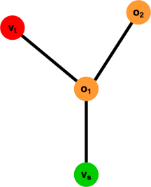
(a)

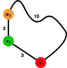
(b)

Figure 3: LABEL:sub@subfig:Acyclic shows a simple connected graph where the objectives have to be visited twice to visit all destinations. LABEL:sub@subfig:BadHamiltonian shows the case where revisiting the source $v_{\text{s}}$ allows a shorter path when triangular inequality does not hold.

2.3 Multi-objective Path Planners and Traveling Salesman Problem

Determining the travel order of nodes in an undirected graph with known edge weights is referred to as a Traveling Salesman Problem (TSP). The TSP is a classic NP-hard problem about finding a shortest possible cycle that visits every node exactly once and returns to the start node [5, 4]. Another variant of TSP, called the shortest Hamiltonian path problem[4], is to find the shortest path that visits all nodes exactly once between a fixed starting node ($v_{s}$) and a fixed terminating node ($v_{t}$). The problem can be solved as a standard TSP problem by assigning sufficiently large negative cost to the edge between $v_{s}$ and $v_{t}$ [4, 5].

We are inspired by the work of [13, 11], where the authors propose to solve the problem through a single-phase algorithm in simulated continuous configuration spaces. They first leverage multiple random trees to solve the multi-goal path planning problem and then solve the TSP via an open-source solver. In particular, they assume that the paths between nodes in the continuous spaces can be constructed in single pass and that the resulting graph can always form a cycle in their simulation environment. Thus, the problem can then be solved by a traditional TSP solver. In practice, however, the graph might not form a cycle (e.g., an acyclic graph or a forest) as shown in Fig. 3a, and even if the graph is cyclic or there exists a Hamiltonian path, there is no guarantee the path is the shortest. In Fig. 3b, the Hamiltonian path simply is $v_{s}\rightarrow o_{1}\rightarrow v_{t}$, and the traversed distance is $12$. However, another shorter path exists if we are allowed to traverse a node ($v_{s}$ in this case) more than once: $v_{s}\rightarrow o_{1}\rightarrow v_{s}\rightarrow v_{t}$ and the distance is $7$. We therefore propose a polynomial-time solver for this relaxed TSP problem; see Sec. 4 for further discussion.

3 Informable Multi-objecticve and Multi-directional RRT^∗

This section introduces an anytime informable multi-objective and multi-directional Rapidly-exploring Random Tree^∗ ($\text{IMOMD-RRT}^{*}$) algorithm as a real-time means to quickly construct from a large-scale map a weighted undirected graph that meets the existence constraint (the solution trajectory must pass by all the objectives at least once), and the order constraint (with fixed starting point and end point). In other words, the $\text{IMOMD-RRT}^{*}$ forms a simple connected graph containing the objectives, source, and target.

3.1 Standard $\text{RRT}^{*}$ Algorithm

The original $\text{RRT}^{*}$ [28] is a sampling-based planner with guaranteed asymptotic optimality in continuous configuration spaces. In general, $\text{RRT}^{*}$ grows a tree where nodes are connected by edges of linear path segments. Additionally, $\text{RRT}^{*}$ considers nearby nodes of a newly extended node when choosing the best parent node and when rewiring the graph to find shorter paths for asymptotic optimality.

3.2 Multi-objective and Multi-directional $\text{RRT}^{*}$ on Graphs

In this paper, we use map to refer to the input graph, which might contain millions of nodes, and use graph to refer to the graph composed of only the destinations including the source and target node. The proposed $\text{IMOMD-RRT}^{*}$ differs from the original $\text{RRT}^{*}$ in six aspects when growing a tree. First, the sampling is performed by picking a random $v_{\text{rand}}$ in the map, and not from an underlying continuous space. The goal bias is not only applied to the target but also the source and all the objectives. Second, a steering function directly finds the closest expandable node as $v_{\text{new}}$ to the random node $v_{\text{rand}}$, without finding the nearest node in the tree, as shown in Fig. 4a. Note that instead of directly sampling from the set of expandable nodes, sampling from the map ameliorates the bias of sampling on the explored area. Third, the parent node is chosen from the nodes connected with the new node $v_{\text{new}}$, called the neighbor nodes. Among the neighbor nodes, the node that yields the lowest path cost from the root becomes the new node’s parent. Fourth, the jumping point search algorithm [26] is also leveraged to speed up tree exploration. Fifth, the $\text{IMOMD-RRT}^{*}$ rewires the neighborhood nodes to minimize the accumulated cost from the root of a tree to $v_{\text{new}}$, as shown in Fig. 4b. Lastly, if $v_{\text{new}}$ belongs to more than one tree, this node is considered a connection node, which connects the path between destinations, as shown in Fig. 5.

(a)

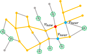
(b)

Figure 4: Illustration of tree expansion and connection nodes of a tree. The unexplored paths in the graph and the spanning tree are represented by the gray and yellow lines, respectively. The green-dashed circles are the expandable nodes. LABEL:sub@subfig:expandable shows the tree $\mathcal{T}_{i}$ extends to the $v_{\text{rand}}$ by growing a node $v_{\text{new}}$ to the closest expandable node. LABEL:sub@subfig:rewiring shows the updated set $\mathcal{X}_{i}$ of expandable nodes and the tree is rewired around the $v_{\text{new}}$. The rewired nodes $v_{\text{near}}$ are represented as the blue dots.

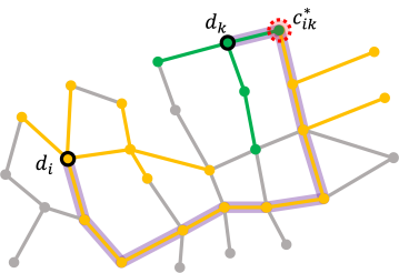
(a)

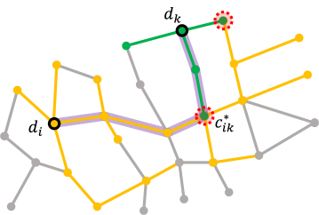
(b)

Figure 5: Illustration of better connection nodes resulting in a better path. Two trees rooted at $d_{i}$ and $d_{k}$ are marked in yellow and green, respectively. The highlighted purple line shows the shortest path between $d_{i}$ and $d_{k}$. The newly extended node $v_{\text{new}}$ (dashed-red circles) is added to a set of connection nodes $\mathcal{C}_{ik}$. The element of the distance matrix, $A_{ik}$, and the connection node $c_{ik}^{*}$ that generates the shortest path between the destination $d_{i}$ and $d_{k}$ are updated as a shorter path is found.

Our proposed graph-based $\text{RRT}^{*}$ modification is summarized below with notation that generally follows graph theory [44]. A graph $\mathcal{G}$ is an ordered triple $(\mathcal{V}(\mathcal{G}),\mathcal{E}(\mathcal{G}),\Phi_{\mathcal{G}})$, where $\mathcal{V}(\mathcal{G})=\{v\in\zeta\}$ is a set of nodes in the robot state space $\zeta$, $\mathcal{E}(\mathcal{G})$ is a set of edges (disjoint from $\mathcal{V}(\mathcal{G})$), and an indication function $\Phi_{\mathcal{G}}$ that associates each edge of $\mathcal{G}$ with an unordered pair (not necessarily distinct) of nodes of $\mathcal{G}$.

Given a set of destinations $\mathcal{D}=\{d_{i}|d_{i}\in\{v_{s},v_{t}\}\cup\mathcal{O}\}_{i=1}^{m+2}$, where $v_{s}\in\mathcal{V}(\mathcal{G})$ is the source node, $v_{t}\in\mathcal{V}(\mathcal{G})$ is the target node, and $\mathcal{O}\subseteq\mathcal{V}(\mathcal{G})$ is the set of $m$ objectives, the $\text{IMOMD-RRT}^{*}$ solves the multi-objective planning problem by growing a tree $\mathcal{T}_{i}=(V,E)$, where $V\subseteq\mathcal{V}(\mathcal{G})$ is a set of nodes connected by edges $E\subseteq\mathcal{E}(\mathcal{G})$, at each of the destinations $d_{i}\in\mathcal{D}$. Thus, it leads to a family of trees $\mathcal{T}=\{\mathcal{T}_{1},\cdots,\mathcal{T}_{m},\mathcal{T}_{m+1},\mathcal{T}_{m+2}\}$.

The proposed $\text{IMOMD-RRT}^{*}$ explores the graph $\mathcal{G}$ by random sampling from $\mathcal{V}(\mathcal{G})$ and extending nodes to grow each tree. We explain a few important functions of IMOMD-RRT^∗ below.

3.2.1 Tree Expansion

Let ${\mathcal{N}(v)}$ be the set of nodes directly connected with a node, i.e., the neighborhood of a node $v$ [44]. A node is expandable if there exists at least one unvisited node connected and at least one node of the tree connected, shown as the dashed-green circles in Fig 4a. Let $\mathcal{X}_{i}$ be the set of expandable nodes of the tree $\mathcal{T}_{i}$. A random node $v_{\text{rand}}$ is sampled from the nodes of the graph $\mathcal{V}(\mathcal{G})$. Next, find the nearest node $v_{\text{new}}$ in the set of expandable nodes $\mathcal{X}_{i}$:

$$v_{\text{new}}=\underset{v\in\mathcal{X}_{i}}{\operatorname*{arg\,min}}\,\mathtt{Dist}(v,v_{\text{rand}}),$$ (1)

where $\mathtt{Dist(\cdot,\cdot)}$ is the distance between two states. Next, the jumping point search algorithm[26] is utilized to speed up the tree expansion. If the current $v_{\text{new}}$ has only one neighbor that is not already in the tree, $v_{\text{new}}$ is added to the tree and that one neighbor is selected as the new $v_{\text{new}}$. This process continues until $v_{\text{new}}$ has at least two neighbors that are not in tree, or it reaches $v_{\text{rand}}$.

3.2.2 Parent Selection

Let the set $\mathcal{N}_{i}({v_{\text{new}})}$ be the neighborhood of the $v_{\text{new}}$ in the tree $\mathcal{T}_{i}$. The node $v_{\text{near}}$ in $\mathcal{N}_{i}({v_{\text{new}})}$ that results in the smallest cost-to-come, $\mathtt{Cost(\cdot,\cdot)}$, is the parent of the $v_{\text{new}}$ and is determined by:

$$v_{\text{parent}}=\underset{v_{\text{near}}\in\mathcal{N}_{i}({v_{\text{new}})}}{\operatorname*{arg\,min}}\{\mathtt{Cost}(\mathcal{T}_{i},v_{\text{near}})+\mathtt{Dist}(v_{\text{near}},v_{\text{new}})\}.$$ (2)

Next, all the unvisted nodes in $\mathcal{N}_{i}({v_{\text{new}})}$ are added to the set of expandable nodes $\mathcal{X}_{i}$.

3.2.3 Tree Rewiring

After the parent node is chosen, the nearby nodes are rewired if a shorter path reaching the node through the $v_{\text{new}}$ is found, as shown in Fig. 4b. The rewiring step guarantees asymptotic optimality, as with the classic algorithm.

3.2.4 Update of Tree Connection

A node is a connection node if it belongs to more than one tree. Let $\mathcal{C}_{ik}$ be the set of connection nodes between $\mathcal{T}_{i}$ and $\mathcal{T}_{k}$, and let $c_{ik}^{*}$ denote the node that connects $\mathcal{T}_{i}$ and $\mathcal{T}_{k}$ with the shortest distance

$$c_{ik}^{*}=\underset{c\in\mathcal{C}_{ik}}{\operatorname*{arg\,min}}~{}\{\mathtt{Cost}(\mathcal{T}_{i},c)+\mathtt{Cost}(\mathcal{T}_{k},c)\}.$$ (3)

Let $A_{(m+2)\times(m+2)}$ be a distance matrix that represents pairwise distances between the destinations, where $m$ is the number of objectives. The element $A_{i,k}$ indicates the shortest path between destinations $d_{i}$ and $d_{k}$, as shown in Fig. 5b. $A_{i,k}$ is computed as

$$A_{i,k}=\mathtt{Cost}(\mathcal{T}_{i},c_{ik}^{*})+\mathtt{Cost}(\mathcal{T}_{k},c_{ik}^{*}).$$ (4)

3.3 Discussion of Informability

As mentioned in Sec. 1, applications such as robotic inspection or vehicle routing might consider prior knowledge of the path, so that the robot can examine certain equipment or area of interests or avoid certain areas in a factory. The prior knowledge can be naturally provided as a number of “pseudo destinations” or samples in the $\text{IMOMD-RRT}^{*}$. A pseudo destination is an artificial destination to help $\text{IMOMD-RRT}^{*}$ to form a connected graph. However, unlike true destinations that will always be visited, a pseudo destination might not be visited after rewiring, as shown in Fig. 6. Prior knowledge through pseudo destinations can also be leveraged to traverse challenging topology, such as bug-traps; see Sec. 5.

Remark 3.1.

One can decide if the order of the pseudo destinations should be fixed or even the pseudo destinations should be objectives (i.e., they will not be removed in the rewiring process.).

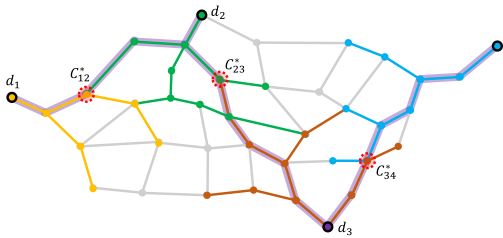
(a)

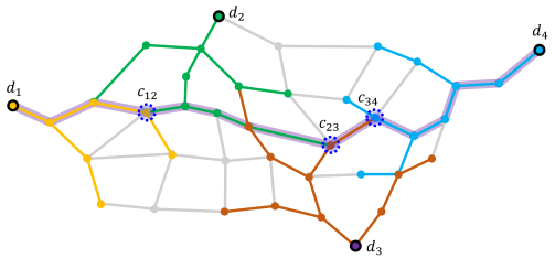
(b)

Figure 6: Illustration of the rewired path of pseudo-destinations. $d_{1}-d_{4}$ are the destinations and marked in different colors. The dashed-red circles are the connection nodes between two trees. The thick purple line is the final path. LABEL:sub@subfig:real_destinations shows the resulting path as if $d_{1}-d_{4}$ are “true” destinations, and LABEL:sub@subfig:pseudo_destinations is the resulting path as if $d_{2}-d_{3}$ are “pseudo” destinations. The real destinations have to be visited as shown in LABEL:sub@subfig:real_destinations, whereas pseudo destinations are artificial destinations to help form a connected graph, and might no longer be visited after rewiring

4 Enhanced Cheapest Insertion and Genetic Algorithm

This section introduces a polynomial-time solver for the relaxed traveling salesman problem (R-TSP).

4.1 Relaxed Traveling Salesman Problem

The R-TSP differs from standard TSP[5, 4, 45] in two perspectives. First, nodes are allowed to be visited more than once, as mentioned in Sec. 2.3. Second, we have a source node where we start and a target node where we end. Therefore, the R-TSP can also be considered a relaxed Hamiltonian path problem[4, 45]. We propose the ECI-Gen solver, which consists of an enhanced version of the cheapest insertion algorithm [15] and a genetic algorithm [16, 17, 18] to solve the R-TSP. The complexity of the proposed solver is $O(N^{3})$, where $N$ is the cardinality of the destination set $\mathcal{D}$.

4.2 Graph Definitions and Connectivity

In graph theory [46, 44], a graph is simple or strict if it has no loops and no two edges join the same pair of nodes. In addition, a path is a sequence of nodes in the graph, where consecutive nodes in the sequence are adjacent, and no node appears more than once in the sequence. A graph is connected if and only if there is a path between each pair of destinations. Once all the destinations form a simple-connected graph, there exists at least one path $\pi$ that passes all destinations $\mathcal{D}$. We can then consider the problem as an R-TSP (see Sec. 4.1), where we have a source and target node as well as several objectives to be visited. Therefore, we impose the graph connectivity and simplicity as sufficient conditions to solve the R-TSP. The disjoint-set data structure [47, 48] is implemented to verify the connectivity of a graph.

4.3 Enhanced Cheapest Insertion Algorithm

The regular cheapest insertion algorithm[15] provides an efficient means to find a sub-optimal sequence that guarantees less than twice the optimal sequence cost. However, it does not handle the case where revisiting the same node makes a shorter sequence. Therefore, we propose an enhanced version of the cheapest insertion algorithm, which comprises of a set of actions: 1) in-sequence insertion, $\lambda_{\text{in-sequence}}$, which is the regular cheapest insertion; 2) in-place insertion, $\lambda_{\text{in-place}}$, to allow the algorithm to revisit existing nodes; and 3) swapping insertion, $\lambda_{\text{swapping}}$, which is inspired by genetic algorithms. Finally, sequence refinement is performed at the end of the algorithm.

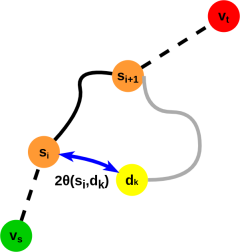
(a)

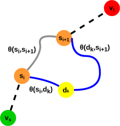
(b)

Figure 7: Illustration of the insertion cost. LABEL:sub@fig:inplace shows the in-place insertion and the resulting sequence contains duplicated $s_{i}$. LABEL:sub@fig:insequence shows the in-sequence insertion without a duplicated element.

Let the current sequence be $\mathcal{S}_{\text{current}}=\{v_{s},s_{1},\cdots,s_{i},s_{i+1},\cdots,s_{n},v_{t}\}$ to indicate the visiting order of destinations, where $s_{\{\cdot\}}\in\mathcal{D}$ and $(n+2)$ is the number of destinations in the sequence. The travel cost $\theta(\cdot,\cdot)$ is the path distance between two destinations provided by the $\text{IMOMD-RRT}^{*}$. The $\mathcal{S}_{\text{current}}$ is constructed by Dijkstra’s algorithm on the graph.

Remark 4.1.

$\mathcal{S}_{\text{current}}$ possibly contains duplicated elements and $s_{i}$ is not necessary $d_{i}$. Therefore, the number of destinations in the sequence $n$ may be larger than the actual number of destinations $m$. Fig. 7a shows the duplicated case with $\mathcal{S}_{\text{current}}=\{v_{s},s_{1},\cdots,s_{i},d_{k},s_{i},s_{i+1},\cdots,s_{n},v_{t}\}$, where $s_{i}$ is duplicated. Figure 7b illustrates an unduplicated case where $\mathcal{S}_{\text{current}}=\{v_{s},s_{1},\cdots,s_{i},d_{k},s_{i+1},$
$\cdots,s_{n},v_{t}\}$.

Let $\mathcal{K}$ denote the set of destinations to be inserted, and let the to-be-inserted destination be $d_{k}$ and its ancestor be $s_{i}$, where $d_{k}\in\mathcal{K}$ and $s_{i}\in\mathcal{S}_{\text{current}}$. Given a current sequence $\mathcal{S}_{\text{current}}$, the location to insert $s^{*}$, and the action of insertion $\lambda^{*}$ are determined by

$$\lambda^{*},s^{*}=\operatorname*{arg\,min}_{\begin{subarray}{c}\lambda_{j}\in\Lambda\\ s_{i}\in\mathcal{S}_{\text{current}}\end{subarray}}\lambda_{j}(s_{i},d_{k}),$$ (5)

where $\Lambda=\{\lambda_{\text{in-sequence}},\lambda_{\text{in-place}},\lambda_{\text{swapping}}\}$ is the set of the insertion actions.

4.3.1 In-place Insertion $\lambda_{\text{in-place}}$

This step detours from $s_{i}$ to $d_{k}$, and the resulting sequence is $\mathcal{S}_{\text{modified}}=\{v_{s},s_{1}\cdots,s_{i},d_{k},s_{i},s_{i+1},\cdots,s_{n},v_{t}\}$, as shown in Fig. 7a. The insertion distance is

$$\lambda_{\text{in-place}}(s_{i},d_{k})=2\theta(s_{i},d_{k}).$$ (6)

4.3.2 In-sequence Insertion $\lambda_{\text{in-sequence}}$

This step inserts $d_{k}$ between $s_{i}$ and $s_{i+1}$ ($\forall s_{i}\in\{\mathcal{S}_{\text{current}}/(v_{t})\}$), and the resulting sequence is $\mathcal{S}_{\text{modified}}=\{v_{s},s_{1},\cdots,s_{i},d_{k},s_{i+1},\cdots,s_{n},v_{t}\}$, as shown in Fig. 7b. The insertion distance is

$$\lambda_{\text{in-sequence}}(s_{i},d_{k})=\theta(s_{i},d_{k})+\theta(d_{k},s_{i+1})-\theta(s_{i},s_{i+1}).$$ (7)

4.3.3 Swapping Insertion $\lambda_{\text{swapping}}$

The swapping insertion changes the order of nodes right next to the newly inserted node. There are three cases in swapping insertion: swapping left, right, or both. For the case of swapping left, the modified sequence is $\mathcal{S}_{\text{modified}}=\{v_{s},s_{1}\cdots,s_{i-2},s_{i},s_{i-1},d_{k},s_{i+1},\cdots,s_{n},$
$v_{t}\}$ by inserting $d_{k}$ between $s_{i}$ and $s_{i+1}$ ($\forall s_{i}\in\{\mathcal{S}_{\text{current}}/(v_{s},s_{1})\}$), and then swapping $s_{i}$ and $s_{i-1}$. The insertion distance of swapping left is

$$\lambda_{\text{swapping (left)}}(s_{i},d_{k}) =\theta(d_{k},s_{i+1})-\theta(s_{i},s_{i+1})$$ (8)

$$+\theta(s_{i-1},d_{k})+\theta(s_{i-2},s_{i})$$

$$-\theta(s_{i-2},s_{i-1}).$$

The right swap is a similar operation except that it swaps $s_{i+1}$ and $s_{i+2}$ instead. Lastly, the case of swapping both does a left swap ($s_{i}$ and $s_{i+1}$) and then a right swap ($s_{i+1}$ and $s_{i+2}$).

4.3.4 Sequence Refinement

In-place insertion occurs when the graph is not cyclic or the triangular inequality does not hold on the graph. The in-place insertion could generate redundant revisited nodes in the final result and lead to a longer sequence. We further refine the sequence by skipping revisited destination when the previous destination and the next destination are connected. The refined sequence of destinations, $\mathcal{S}_{\text{ECI}}$, with cardinality $r\leq n$ is the input to the genetic algorithm.

4.4 Genetic Algorithm

We further leverage a genetic algorithm [16, 17, 18] to refine the sequence from the enhanced cheapest insertion algorithm. The genetic algorithm selects a parent sequence and then generates a new offspring sequence from it by either a mutation or crossover process.

In brief, we first take the ordered sequence $\mathcal{S}_{\text{ECI}}$ from the enhanced cheapest insertion as our first and only parent for the mutation process, which produces multiple offspring. Only the offspring with a lower cost than the parent are considered the parents for the crossover process.

1) Mutation: There are three steps for each mutation process, as described in Fig. 8a. First, the ordered sequence $\mathcal{S}_{\text{ECI}}$ from the enhanced cheapest insertion is randomly divided into $k$ segments. Second, random inversion is executed for each segment except the first and last segments, which contain the source and the target. Lastly, the segments in the middle are randomly reordered and spliced together. Let the resulting offspring sequence be $\psi=\{v_{s},p_{1},p_{2},\cdots,p_{r},v_{t}\}$, where $v_{s}$ is the source node, $v_{t}$ is the target node, $(r+2)$ is the number of destinations in the sequence (the same cardinality of $S_{\text{ECI}}$), and $\{p_{i}\}_{i=1}^{r}$ is the re-ordered destinations, which could possibly contain the start and end. The cost $\Theta$ of the offspring is computed as

$$\Theta=\theta(v_{s},p_{1})+\sum_{i=1}^{r}\theta(p_{i},p_{i+1})+\theta(p_{n},v_{t}),$$ (9)

where $\theta(\cdot,\cdot)$ is the path distance between two destinations provided by the $\text{IMOMD-RRT}^{*}$.

We perform the mutation process thousands of times, resulting in thousands of offspring. Note that only the offspring with a lower cost than the cost of the parent are kept for the crossover process.

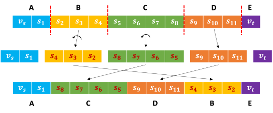
(a) Mutation

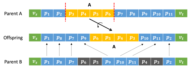
(b) Crossover

Figure 8: Illustration of the mutation and crossover in the Genetic Algorithm. LABEL:sub@fig:Mutation In mutation, the sequence is randomly cut into five segments and each segment is randomly reversed except Segment A and Segment E. In this case, Segment B and C are reversed and D does not. Finally, the modified segments are spliced in random order and resulting an offspring ACDBE. LABEL:sub@fig:Crossover In crossover, two sequences (Parent A and Parent B) are picked from the offspring from the mutation process. A sub-sequence of one of the two sequences is randomly selected (Sub-sequence A in this case). Next, random inversion is performed on Sub-sequence A and the resulting segment is randomly placed inside an empty sequence of the offspring. Lastly, the remaining elements of the offspring are filled by the order of the other sequence (Parent B) except the elements that are already in the offspring sequence.

2) Crossover: Let the set of mutated sequences from the mutation process be $\Psi=\{\psi_{i}\}_{i=1}^{h}$, where $h$ is the number of offspring kept after the mutation process. For each generation, the crossover process is performed thousands of times and only the offspring with a lower cost than the previous generation are kept. Each crossover process combines sub-sequences of any two sequences ($\psi_{i},\psi_{j}\in\Psi$) to generate a new offspring, as described in Fig.8b. The probability of a sequence $\psi_{i}$ being picked is defined as:

$$P_{\psi}(\psi=\psi_{i})=\frac{\rho_{i}}{\sum_{i=1}^{w}\rho_{i}},~{}~{}\rho_{i}=\frac{1}{\Theta_{i}},$$ (10)

where $w$ is the number of the remaining offspring from each generation after the $(i-1)^{\text{th}}$ generation and $\rho_{i}$ is the fitness of the sequence $\psi_{i}$. Given the two selected sequences and an empty to-be-filled offspring, a segment of one of the two sequences is randomly selected, and random inversion is performed on the segment. The resulting segment is randomly placed inside the empty sequence of the offspring. Lastly, the remaining elements of the offspring are filled by the order of the other sequence except the elements that are already in the offspring sequence. After a few generations, the offspring with the lowest cost, $\psi^{*}$, is the final sequence $\mathcal{S}_{\text{ECI-Gen}}$ of the destinations.

Remark 4.2.

Whenever the IMOMD-RRT^∗ provides a better path (due to its asymptotic optimality), the ECI-Gen solver will be executed to solve for a better visiting order of the destinations. Therefore, the full system provides paths with monotonically improving path cost in an anytime fashion.

4.5 Discussion of time complexity

As mentioned in Sec. 4.3, the first sequence $\mathcal{S}_{\text{current}}$ is constructed by Dijkstra’s algorithm, which is an $O(N^{2})$ process, where $N$ is the cardinality of the destination set $\mathcal{D}$. We then pass the sequence to the enhanced cheapest insertion algorithm, whose time complexity is $O(N^{3})$, to generate a set of parents for the genetic algorithm, which is also an $O(N^{3})$ process. Therefore, the overall time complexity of the proposed ECI-Gen solver is $O(N^{3})$, and indeed a polynomial solver.

5 Experimental Results

This section presents extensive evaluations of the $\text{IMOMD-RRT}^{*}$ system applied to two complex vehicle routing scenarios. The robot state $\zeta$ is defined as latitude and longitude. The distance between robot states $\mathtt{Dist}(\cdot,\cdot)$ in (1) is defined as the haversine distance[49]. We implemented the bi-directional A^∗ [20] and ANA^∗ [21] as our baselines to compare the speed and memory usage (the number of explored nodes). We evaluate the IMOMD-RRT^∗ system (IMOMD-RRT^∗ and the ECI-Gen solver) on a large and complex map of Seattle, USA. The map contains $1,054,372$ nodes and $1,173,514$ edges, and is downloaded from OpenStreetMap (OSM), which is a public map service built for real applications. We then place $25$ destinations in the map. We demonstrate that the $\text{IMOMD-RRT}^{*}$ system is able to concurrently find paths connecting destinations and determine the order of destinations. We also show that the system escapes from a bug trap by inherently receiving prior knowledge. The algorithm runs on a laptop equipped with Intel${}^{\text{\textregistered}}$ Core${}^{\text{TM}}$ i7-1185G7 CPU @ 3.00 GHz.

To show the performance and ability of multi-objective and determining the visiting order, we randomly set $25$ destinations in the Seattle map. There are 25! possible combinations of visiting orders and therefore it is intractable to solve the visiting order by brute force. The results are shown in Fig. 9, where $\text{IMOMD-RRT}^{*}$ finds the first path faster than both Bi-A^∗ and ANA^∗ with a lower cost and then also spends less time between solution improvements. Additionally, the memory usage of $\text{IMOMD-RRT}^{*}$ is less than ANA* and much less than bi-A^∗. As shown in Table 1, the proposed system provides the first solution 10 times faster than bi-A^∗ and four time faster than ANA^∗. In addition, the proposed system also consumes 65 times less memory than bi-A^∗ and 4.7 times less memory usage than ANA^∗.

Table 1: Quantitative results of the proposed $\text{IMOMD-RRT}^{*}$ system on two large maps (both graphs contain more than one million nodes and edges) built for real robotics and vehicle applications. The proposed system outperforms bi-A^∗ and ANA^∗.

		Initial Solution Time [seconds]	Initial Path Cost [kilometers]	Final Memory Usage [# explored nodes]
Seattle	IMOMD-RRT∗	0.44	501,342	49,768
	Bi-A∗	4.40	808,416	3,240,515
	ANA∗	1.70	1,089,873	234,457
San Francisco	IMOMD-RRT∗	1.10	156,807	61,785
	Bi-A∗	9.93	315,061	3,640,863
	ANA∗	Failed	Failed	Failed

Prior knowledge through pseudo destinations can also be leveraged to traverse challenging topology, such as bug-traps[50]. This problem is commonly seen in man-made environments such as a neighborhood with a single entry or cities separated by a body of water, as in Fig. 10. As mentioned in Remark 3.3, prior knowledge is provided as a number of pseudo destinations in the $\text{IMOMD-RRT}^{*}$ as a prior collision-free path in the graph for robotics inspection or vehicle routing. Next, the prior path is then being rewired by the $\text{IMOMD-RRT}^{*}$ to improve the path. We demonstrate this feature by providing the prior knowledge to escape the bug trap in San Francisco, as shown in Fig. 10. The map contains $1,277,702$ nodes and $1,437,713$ edges. As shown in Table 1, the proposed system escapes from the trap nine times faster than bi-A^∗, whereas ANA^∗ failed to provide a path within the given time frame. The proposed system also consumes 58.9 times less memory than bi-A^∗.

In summary, we developed an anytime iterative system to provide paths between multiple objectives by the $\text{IMOMD-RRT}^{*}$ and to determine the visiting order of the objectives by the ECI-Gen solver solver in polynomial time. We also demonstrate that the proposed system is able to inherently accommodate prior information to escape from challenging topology.

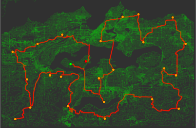
(a)

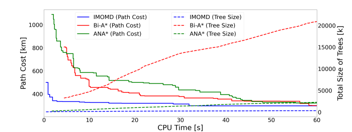
(b)

Figure 9: Quantitative and qualitative results for an OSM of Seattle, where we have 25 destinations to be visited. The proposed $\text{IMOMD-RRT}^{*}$ outperforms Bi-A^∗ and ANA^∗ in term of speed and memory usage (the number of explored nodes).

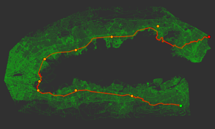
(a)

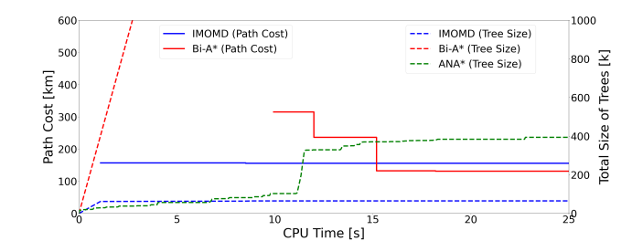
(b)

Figure 10: Providing prior knowledge to the proposed $\text{IMOMD-RRT}^{*}$ system to avoid bug traps. The left and the right are the qualitative and quantitative results for a bug trap in San Francisco, respectively. We have eight pseudo destinations to help escape the challenging topology, where the source and target are separated by a body of water. Note that ANA^∗ failed to provide a solution in the given time.

6 Conclusion and Future Work

We presented an anytime iterative system on large-complex graphs to solve the multi-objective path planning problem, to decide the visiting order of the objectives, and to incorporate prior knowledge of the potential trajectory. The system is comprised of an anytime informable multi-objective and multi-directional RRT^∗ to connect the destinations to form a connected graph and the ECI-Gen solver to determine the visiting order (via a relaxed Traveling Salesman Problem) in polynomial time.

The system was extensively evaluated on OpenStreetMap (OSM), built for autonomous vehicles and robots in practice. In particular, the system solved a path planning problem and the visiting order with $25$ destinations ($25!$ possible combinations of visiting orders) on an OSM of Seattle, containing more than a million nodes and edges, in 0.44 seconds. In addition, we demonstrated the system is able to leverage a reference path (prior knowledge) to navigate challenging topology for robotics inspection or vehicle routing applications. All the evaluations show that our proposed method outperforms the Bi-A^∗ and ANA^∗ algorithm in terms of speed and memory usage.

In the future, we shall use the developed system within autonomy systems[51, 52, 53, 54, 55, 56, 57, 58, 59, 30, 60, 61, 62] on a robot to perform point-to-point tomometric navigation in graph-based maps while locally avoiding obstacles and uneven terrain. It would also be interesting to deploy the system with multi-layered graphs and maps [63, 64, 65] to incorporate different types of information.

References

- [1] J. Faigl and G. A. Hollinger, “Unifying multi-goal path planning for autonomous data collection,” in 2014 IEEE/RSJ International Conference on Intelligent Robots and Systems. IEEE, 2014, pp. 2937–2942.
- [2] H. Hu, K. Xiong, G. Qu, Q. Ni, P. Fan, and K. B. Letaief, “Aoi-minimal trajectory planning and data collection in uav-assisted wireless powered iot networks,” IEEE Internet of Things Journal, vol. 8, no. 2, pp. 1211–1223, 2020.
- [3] M. Samir, S. Sharafeddine, C. M. Assi, T. M. Nguyen, and A. Ghrayeb, “Uav trajectory planning for data collection from time-constrained iot devices,” IEEE Transactions on Wireless Communications, vol. 19, no. 1, pp. 34–46, 2019.
- [4] M. Jünger, G. Reinelt, and G. Rinaldi, “The traveling salesman problem,” Handbooks in operations research and management science, vol. 7, pp. 225–330, 1995.
- [5] D. L. Applegate, R. E. Bixby, V. Chvátal, and W. J. Cook, The traveling salesman problem. Princeton university press, 2011.
- [6] C. Ma, R. He, and W. Zhang, “Path optimization of taxi carpooling,” PLoS One, vol. 13, no. 8, p. e0203221, 2018.
- [7] H. Huang, D. Bucher, J. Kissling, R. Weibel, and M. Raubal, “Multimodal route planning with public transport and carpooling,” IEEE Transactions on Intelligent Transportation Systems, vol. 20, no. 9, pp. 3513–3525, 2018.
- [8] A. O. Al-Abbasi, A. Ghosh, and V. Aggarwal, “Deeppool: Distributed model-free algorithm for ride-sharing using deep reinforcement learning,” IEEE Transactions on Intelligent Transportation Systems, vol. 20, no. 12, pp. 4714–4727, 2019.
- [9] S. Hulagu and H. B. Celikoglu, “An electric vehicle routing problem with intermediate nodes for shuttle fleets,” IEEE Transactions on Intelligent Transportation Systems, 2020.
- [10] OpenStreetMap contributors, “Planet dump retrieved from https://planet.osm.org ,” https://www.openstreetmap.org, 2017.
- [11] J. Janos, V. Vonásek, and R. Penicka, “Multi-goal path planning using multiple random trees,” IEEE Robotics and Automation Letters, vol. 6, no. 2, pp. 4201–4208, 2021.
- [12] D. Devaurs, T. Siméon, and J. Cortés, “A multi-tree extension of the transition-based rrt: Application to ordering-and-pathfinding problems in continuous cost spaces,” in 2014 IEEE/RSJ International Conference on Intelligent Robots and Systems. IEEE, 2014, pp. 2991–2996.
- [13] V. Vonásek and R. Penicka, “Space-filling forest for multi-goal path planning,” in 2019 24th IEEE International Conference on Emerging Technologies and Factory Automation (ETFA). IEEE, 2019, pp. 1587–1590.
- [14] B. Englot and F. Hover, “Multi-goal feasible path planning using ant colony optimization,” in 2011 IEEE International Conference on Robotics and Automation. IEEE, 2011, pp. 2255–2260.
- [15] D. J. Rosenkrantz, R. E. Stearns, and P. M. Lewis, II, “An analysis of several heuristics for the traveling salesman problem,” SIAM journal on computing, vol. 6, no. 3, pp. 563–581, 1977.
- [16] J.-Y. Potvin, “Genetic algorithms for the traveling salesman problem,” Annals of Operations Research, vol. 63, no. 3, pp. 337–370, 1996.
- [17] C. Moon, J. Kim, G. Choi, and Y. Seo, “An efficient genetic algorithm for the traveling salesman problem with precedence constraints,” European Journal of Operational Research, vol. 140, no. 3, pp. 606–617, 2002.
- [18] H. Braun, “On solving travelling salesman problems by genetic algorithms,” in International Conference on Parallel Problem Solving from Nature. Springer, 1990, pp. 129–133.
- [19] Z. H. Ahmed, “Genetic algorithm for the traveling salesman problem using sequential constructive crossover operator,” International Journal of Biometrics & Bioinformatics (IJBB), vol. 3, no. 6, p. 96, 2010.
- [20] A. V. Goldberg and C. Harrelson, “Computing the shortest path: A search meets graph theory.” in SODA, vol. 5. Citeseer, 2005, pp. 156–165.
- [21] J. Van Den Berg, R. Shah, A. Huang, and K. Goldberg, “Anytime nonparametric a,” in Twenty-Fifth AAAI Conference on Artificial Intelligence, 2011.
- [22] P. Hart, N. Nilsson, and B. Raphael, “A formal basis for the heuristic determination of minimum cost paths,” IEEE Transactions on Systems Science and Cybernetics, vol. 4, no. 2, pp. 100–107, 1968. [Online]. Available: https://doi.org/10.1109/tssc.1968.300136
- [23] E. W. Dijkstra, “A note on two problems in connexion with graphs,” Numerische mathematik, vol. 1, no. 1, pp. 269–271, 1959.
- [24] M. Likhachev and A. Stentz, “R* search,” University of Pennsylvania, 2008.
- [25] M. Likhachev, G. J. Gordon, and S. Thrun, “Ara*: Anytime a* with provable bounds on sub-optimality,” Advances in neural information processing systems, vol. 16, 2003.
- [26] D. Harabor and A. Grastien, “The jps pathfinding system,” in International Symposium on Combinatorial Search, vol. 3, no. 1, 2012.
- [27] S. M. LaValle et al., “Rapidly-exploring random trees: A new tool for path planning,” Computer Science Dept., Iowa State University, 1998.
- [28] S. Karaman and E. Frazzoli, “Sampling-based algorithms for optimal motion planning,” Int. J. Robot. Res., vol. 30, no. 7, pp. 846–894, 2011.
- [29] S. Karaman, M. R. Walter, A. Perez, E. Frazzoli, and S. Teller, “Anytime motion planning using the rrt*,” in Proc. IEEE Int. Conf. Robot. and Automation, 2011, pp. 1478–1483.
- [30] “Efficient Anytime CLF Reactive Planning System for a Bipedal Robot on Undulating Terrain, author=Jiunn-Kai Huang and Jessy W. Grizzle,” arXiv preprint arXiv:2108.06699, 2021.
- [31] S. Morgan and M. S. Branicky, “Sampling-based planning for discrete spaces,” in 2004 IEEE/RSJ International Conference on Intelligent Robots and Systems (IROS)(IEEE Cat. No. 04CH37566), vol. 2. IEEE, 2004, pp. 1938–1945.
- [32] M. S. Branicky, M. M. Curtiss, J. A. Levine, and S. B. Morgan, “Rrts for nonlinear, discrete, and hybrid planning and control,” in 42nd IEEE International Conference on Decision and Control (IEEE Cat. No. 03CH37475), vol. 1. IEEE, 2003, pp. 657–663.
- [33] K. Solovey, O. Salzman, and D. Halperin, “Finding a needle in an exponential haystack: Discrete rrt for exploration of implicit roadmaps in multi-robot motion planning,” The International Journal of Robotics Research, vol. 35, no. 5, pp. 501–513, 2016.
- [34] R. Shome, K. Solovey, A. Dobson, D. Halperin, and K. E. Bekris, “drrt*: Scalable and informed asymptotically-optimal multi-robot motion planning,” Autonomous Robots, vol. 44, no. 3, pp. 443–467, 2020.
- [35] S.-C. Huang, M.-K. Jiau, and Y.-P. Liu, “An ant path-oriented carpooling allocation approach to optimize the carpool service problem with time windows,” IEEE Systems Journal, vol. 13, no. 1, pp. 994–1005, 2018.
- [36] Y. Duan, T. Mosharraf, J. Wu, and H. Zheng, “Optimizing carpool scheduling algorithm through partition merging,” in 2018 IEEE International Conference on Communications (ICC). IEEE, 2018, pp. 1–6.
- [37] M. Tamannaei and I. Irandoost, “Carpooling problem: A new mathematical model, branch-and-bound, and heuristic beam search algorithm,” Journal of Intelligent Transportation Systems, vol. 23, no. 3, pp. 203–215, 2019.
- [38] H. K. Suman and N. B. Bolia, “Improvement in direct bus services through route planning,” Transport Policy, vol. 81, pp. 263–274, 2019.
- [39] Y. Lyu, C.-Y. Chow, V. C. Lee, J. K. Ng, Y. Li, and J. Zeng, “Cb-planner: A bus line planning framework for customized bus systems,” Transportation Research Part C: Emerging Technologies, vol. 101, pp. 233–253, 2019.
- [40] M. D. Simoni, E. Kutanoglu, and C. G. Claudel, “Optimization and analysis of a robot-assisted last mile delivery system,” Transportation Research Part E: Logistics and Transportation Review, vol. 142, p. 102049, 2020.
- [41] S. Naccache, J.-F. Côté, and L. C. Coelho, “The multi-pickup and delivery problem with time windows,” European Journal of Operational Research, vol. 269, no. 1, pp. 353–362, 2018.
- [42] M. Nazari, A. Oroojlooy, L. Snyder, and M. Takác, “Reinforcement learning for solving the vehicle routing problem,” Advances in neural information processing systems, vol. 31, 2018.
- [43] E. H.-C. Lu and Y.-W. Yang, “A hybrid route planning approach for logistics with pickup and delivery,” Expert Systems with Applications, vol. 118, pp. 482–492, 2019.
- [44] J. A. Bondy, U. S. R. Murty, et al., Graph theory with applications. Macmillan London, 1976, vol. 290.
- [45] A. P. Punnen, “The traveling salesman problem: Applications, formulations and variations,” in The traveling salesman problem and its variations. Springer, 2007, pp. 1–28.
- [46] D. B. West et al., Introduction to graph theory. Prentice hall Upper Saddle River, 2001, vol. 2.
- [47] T. H. Cormen, C. E. Leiserson, R. L. Rivest, and C. Stein, Introduction to algorithms. MIT press, 2022.
- [48] Z. Galil and G. F. Italiano, “Data structures and algorithms for disjoint set union problems,” ACM Computing Surveys (CSUR), vol. 23, no. 3, pp. 319–344, 1991.
- [49] G. Van Brummelen, “Heavenly mathematics,” in Heavenly Mathematics. Princeton University Press, 2012.
- [50] S. M. LaValle, Planning Algorithms. Cambridge, U.K.: Cambridge University Press, 2006, available at http://planning.cs.uiuc.edu/.
- [51] J. Rehder, J. Nikolic, T. Schneider, T. Hinzmann, and R. Siegwart, “Extending kalibr: Calibrating the extrinsics of multiple imus and of individual axes,” in 2016 IEEE International Conference on Robotics and Automation (ICRA). IEEE, 2016, pp. 4304–4311.
- [52] P. Furgale, J. Rehder, and R. Siegwart, “Unified temporal and spatial calibration for multi-sensor systems,” in 2013 IEEE/RSJ International Conference on Intelligent Robots and Systems. IEEE, 2013, pp. 1280–1286.
- [53] L. Oth, P. Furgale, L. Kneip, and R. Siegwart, “Rolling shutter camera calibration,” in Proceedings of the IEEE Conference on Computer Vision and Pattern Recognition, 2013, pp. 1360–1367.
- [54] J. Huang and J. W. Grizzle, “Improvements to Target-Based 3D LiDAR to Camera Calibration,” IEEE Access, vol. 8, pp. 134 101–134 110, 2020.
- [55] J. K. Huang, S. Wang, M. Ghaffari, and J. W. Grizzle, “LiDARTag: A Real-Time Fiducial Tag System for Point Clouds,” IEEE Robotics and Automation Letters, pp. 1–1, 2021.
- [56] J.-K. Huang, W. Clark, and J. W. Grizzle, “Optimal target shape for lidar pose estimation,” IEEE Robotics and Automation Letters, vol. 7, no. 2, pp. 1238–1245, 2021.
- [57] J.-K. Huang, C. Feng, M. Achar, M. Ghaffari, and J. W. Grizzle, “Global Unifying Intrinsic Calibration for Spinning and Solid-State LiDARs,” arXiv preprint arXiv:2012.03321, 2020.
- [58] R. Hartley, M. G. Jadidi, J. Grizzle, and R. M. Eustice, “Contact-aided invariant extended Kalman filtering for legged robot state estimation,” in Proc. Robot.: Sci. Syst. Conf., Pittsburgh, Pennsylvania, June 2018.
- [59] R. Hartley, M. Ghaffari, R. M. Eustice, and J. W. Grizzle, “Contact-aided invariant extended kalman filtering for robot state estimation,” The International Journal of Robotics Research, vol. 39, no. 4, pp. 402–430, 2020.
- [60] Y. Gong and J. Grizzle, “Zero dynamics, pendulum models, and angular momentum in feedback control of bipedal locomotion,” 2021.
- [61] ——, “Angular momentum about the contact point for control of bipedal locomotion: Validation in a lip-based controller,” arXiv preprint arXiv:2008.10763, 2020.
- [62] Y. Gong, R. Hartley, X. Da, A. Hereid, O. Harib, J.-K. Huang, and J. Grizzle, “Feedback control of a cassie bipedal robot: Walking, standing, and riding a segway,” in 2019 American Control Conference (ACC). IEEE, 2019, pp. 4559–4566.
- [63] P. Fankhauser, M. Bloesch, and M. Hutter, “Probabilistic terrain mapping for mobile robots with uncertain localization,” IEEE Robotics and Automation Letters (RA-L), vol. 3, no. 4, pp. 3019–3026, 2018.
- [64] P. Fankhauser, M. Bloesch, C. Gehring, M. Hutter, and R. Siegwart, “Robot-centric elevation mapping with uncertainty estimates,” in International Conference on Climbing and Walking Robots (CLAWAR), 2014.
- [65] L. Gan, R. Zhang, J. W. Grizzle, R. M. Eustice, and M. Ghaffari, “Bayesian spatial kernel smoothing for scalable dense semantic mapping,” IEEE Robotics and Automation Letters, vol. 5, no. 2, pp. 790–797, April 2020.