The Inflaton that Could : Primordial Black Holes and Second Order Gravitational Waves from Tachyonic Instability induced in Higgs-$R^{2}$ Inflation

Abstract

The running of the Higgs self coupling may lead to numerous phenomena in early universe cosmology. In this paper we introduce a scenario where the Higgs running induces turns in the trajectory passing a region with tachyonic mass, leading to a temporal tachyonic growth in the curvature power spectrum. This effect induced by the Higgs leaves phenomena in the form of primordial black holes and stochastic gravitational waves, where proposed GW observatories will be able to probe in the near future.

1 Introduction

We are now officially entering the era of gravitational wave (GW) observatories. After the discovery of GWs from LIGO/VIRGO, the database including gravitational wave signals of binary systems increased significantly [1, 2]. Recently, NANOGrav and several pulsar timing arrays reported a background which may represent a stochastic gravitational wave background [3, 4, 5, 6, 7, 8], where scenarios incorporate solar-mass primordial black holes [9, 10, 11, 12]. Many proposed GW observatories (e.g. LISA [13, 14], DECIGO [15, 16], Einstein Telescope [17], SKA [18], etc.) expect to cover a wide range of frequencies, further unraveling physics occurring in the early universe [19, 20].

Numerous scenarios in our early universe may produce stochastic GW backgrounds (SGWB), which include cases that induce stochastic GWs at the second order (a comprehensive review regarding this topic can be found in [21]). Processes induced by inflation gained much interest with a localized enhancement in the curvature power spectrum [22, 23, 24, 25, 26, 27, 28, 29, 30, 31, 32, 33, 34, 35, 36, 37, 38, 39, 40, 41, 42, 43, 44, 45, 46, 47, 48, 49, 50, 51, 52, 53, 54, 55, 56, 57, 58, 59, 60, 61, 62, 63, 10, 11, 64, 65, 66, 67, 68, 69, 70, 71, 72, 73, 74], in correlation with copious primordial black hole (PBH) production [75, 76, 77, 78].

Among many inflationary models, Higgs inflation [80] and its extensions [81, 82, 83, 84, 85, 86, 87, 88, 89, 90, 91, 92, 93, 94, 95, 96, 97, 98, 99, 100, 101, 102, 103, 104, 105, 106, 107, 108, 53, 109, 110, 63, 111, 112, 113, 114, 115, 116] gain immense interest as it incorporates the Standard Model scalar with a nonminimal coupling to gravity, and it provides the best fit to current cosmic microwave background (CMB) observations. The running behavior of the Standard Model Higgs is also incorporated in the potential, which prospects numerous phenomena in our cosmology [85, 88, 93, 97]. A general setup incorporating this is the Higgs-$R^{2}$ inflation, where two scalars, namely the scalaron and the SM Higgs generate a two field potential [91, 92, 117, 94, 118, 102, 101, 99, 105, 103, 108, 106, 53, 110, 119, 120, 121, 63, 112, 113, 116].

Intriguingly, the running of the Higgs self coupling running can induce much richer phenonema. We discussed the parameters that induce an inflection point in the model describable in the framework of an effective single field case in our previous work [53]. There, we concluded that an enhanced curvature perturbation can be produced by a near-inflection point induced by the Higgs running, resulting in a tight correlation with the PBH mass and the CMB spectral index. In this paper, we revisit the Higgs running and show cases where the inflaton possesses turns in its trajectory and approaches the hill in the potential at $h=0$, which exhibits a tachyonic mass. Isocurvature perturbations grow exponentially, which induce a rapid growth of the curvature perturbations (this mechanism, mainly incorporating a rapid turn in the non-geodesic field space has taken interest in the past several years [57, 58, 59, 62, 63, 122, 72, 123]). This in turn displays a sharp bump in the curvature power spectrum, where this local feature is probe-able in the form of PBHs and stochastic GWs in a wide range of masses and frequencies. The mass and abundance of the PBHs, and correspondingly the energy density and the frequency of the stochastic GWs depend on the parameter choices $(\xi,\lambda)$, which allows one to connect and probe low energy Standard Model measurements with proposed gravitational wave measurements.

This paper is organized as follows, we introduce the Higgs-$R^{2}$ setup including the running behavior of the Higgs. We analyze the background dynamics of the inflaton and classify the trajectory in steps. We then compute the curvature and isocurvature perturbations of the model and its corresponding PBH abundance and GW spectrum. We conclude with the implications of the results.

2 Inflation action

The action for the Higgs-$R^{2}$ inflation in the Jordan frame is given as

$$S_{J}=\int d^{4}x\sqrt{-g_{J}}\left[\frac{M_{P}^{2}}{2}\left(R_{J}+\frac{\xi(\mu)\,h^{2}}{M_{P}^{2}}R_{J}+\frac{R_{J}^{2}}{6M^{2}}\right)-\frac{1}{2}g^{\mu\nu}\nabla_{\mu}h\nabla_{\nu}h-\frac{\lambda(\mu)}{4}h^{4}\right],$$ (2.1)

with the Higgs, $h$, in the unitary gauge, the reduced Planck mass being $M_{P}=1/\sqrt{8\pi G}\simeq 2.44\times 10^{18}~{}{\rm GeV}$, and the scalaron mass $M\mathrel{\hbox to0.0pt{\lower 4.0pt\hbox{\hskip 1.0pt$\sim$}\hss}\raise 1.0pt\hbox{$<$}}M_{P}/\xi$ introduced to match the dimensions. We take the Higgs self coupling running $\lambda\left(\mu\right)$ at a scale $\mu$. The scalaron, $s$, is defined via

$$\sqrt{\frac{2}{3}}\frac{s}{M_{P}}=\ln\left(1+\frac{\xi h^{2}}{M_{P}^{2}}+\frac{R_{J}}{3M^{2}}\right)\equiv\Omega(s).$$ (2.2)

Weyl transformation yields the action in Einstein frame where $g_{\mu\nu}=e^{\Omega(s)}g^{J}_{\mu\nu}$ with two scalar fields, $(\phi^{a})=(s,h)$ appearing in the scalar potential $U(\phi^{a})$. As a consequence, the kinetic terms involve a nontrivial field space metric $G_{ab}$:

$$S=\int d^{4}x\sqrt{-g}\left[\frac{M_{P}^{2}}{2}R-\frac{1}{2}G_{ab}g^{\mu\nu}\nabla_{\mu}\phi^{a}\nabla_{\nu}\phi^{b}-U(\phi^{a})\right],$$ (2.3)

$$U(\phi^{a})\equiv e^{-2\Omega(s)}\left\{\frac{3}{4}M_{P}^{2}M^{2}\left(e^{\Omega(s)}-1-\frac{\xi(\mu)h^{2}}{M_{P}^{2}}\right)^{2}+\frac{\lambda\left(\mu\right)}{4}h^{4}\right\}.$$ (2.4)

Explicitly, the field space metric is given for $(s,h)$ as

$$G_{ab}=\begin{pmatrix}1&&0\\ 0&&e^{-\Omega(s)}\end{pmatrix}.$$ (2.5)

The parameters $\left.(M,\xi,\lambda)\right|_{\mu}$ running in scale $\mu$ by the Standard Model and scalaron interactions follow 1-loop beta functions in the form [124, 125, 126, 127, 128, 101, 108, 110]

$$\beta_{\alpha} =-\frac{1}{16\pi^{2}}\frac{\left(1+6\xi\right)^{2}}{18},$$ (2.6)

$$\beta_{\xi} =+\frac{1}{16\pi^{2}}\left(\xi+\frac{1}{6}\right)\left(12\lambda+6y_{t}^{2}-\frac{3}{2}g^{\prime 2}-\frac{9}{2}g^{2}\right),$$ (2.7)

$$\beta_{\lambda} =\beta_{\text{SM}}+\frac{1}{16\pi^{2}}\frac{2\xi^{2}\left(1+6\xi\right)^{2}M^{4}}{M_{P}^{4}},$$ (2.8)

with $\alpha={M_{P}^{2}}/{12M^{2}}$ and $\beta_{\rm SM}$ being the Standard Model contribution [129]. Choosing the renormalization prescription to be $\mu\simeq\sqrt{h^{2}}$, we perform a standard parameterization of the parameters $\lambda(\mu)\,,\,\,\xi(\mu)$  around the $\lambda$ minimum field value $h_{m}$

$$\left.\lambda\left(\mu\right)\right|_{\mu=h} =\lambda_{m}+\frac{\beta_{2}^{\text{SM}}}{\left(16\pi^{2}\right)^{2}}\ln^{2}\left(\sqrt{\frac{h^{2}}{h_{m}^{2}}}\right)=\lambda_{m}+b\ln^{2}\left(\sqrt{\frac{h^{2}}{h_{m}^{2}}}\right)$$ (2.9)

$$\left.\xi\left(\mu\right)\right|_{\mu=h} =\xi_{0}+2{\beta_{\xi}^{0}}\ln\left(\sqrt{\frac{h^{2}}{h_{m}^{2}}}\right)=\xi_{0}+b_{\xi}\ln\left(\sqrt{\frac{h^{2}}{h_{m}^{2}}}\right)$$ (2.10)

with $\lambda_{m}\equiv\lambda(h_{m})\sim\mathcal{O}(10^{-6})$, $\xi_{0}\equiv\xi(h_{m})\sim\mathcal{O}(1)$ , $\beta_{2}^{\text{SM}}\sim 0.5$, $\beta_{\xi}^{0}\equiv\beta_{\xi}(h_{m})\sim-0.01$, $\mu_{m}=h_{m}\sim 10^{17}-10^{18}\,\,\text{GeV}$ as denoted in [130, 131]. The 1-loop $\beta$-functions indicate that the running effects are most significant in $\lambda$, with many orders changing while running from EW scales to Planck scales, whereas the $\xi$ parameter running is insignificant over this running range maintaining the same order. Throughout the paper we take $M_{P}=1$ and focus on the $h>0$ region unless specified.

3 Background evolution

The action eq. (2.3) yields the equations of motion for the homogeneous background fields and the Friedmann equation with the metric [99]

$$ds^{2}=-dt^{2}+a(t)^{2}\delta_{ij}dx^{i}dx^{j}$$ (3.1)

gives, expressed incorporating the ‘curved field space metric’ effects,

$$D_{t}\dot{\phi}^{a}+3H\dot{\phi}^{a}+G^{ab}D_{b}U =0,$$ (3.2)

$$3H^{2} =\frac{1}{2}\dot{\phi}_{0}^{2}+U$$ (3.3)

with the covariant derivatives $D_{a}\phi^{b}=\partial_{a}\phi^{b}+\Gamma^{b}_{ca}\phi^{c}$, $\Gamma^{b}_{ca}=\frac{1}{2}G^{be}\left(\partial_{c}G_{ae}+\partial_{a}G_{ec}-\partial_{e}G_{ca}\right)$, $D_{t}X^{a}=\dot{X}^{a}+\Gamma_{bc}^{a}\dot{\phi}^{b}X^{c}$, and $\dot{\phi}_{0}^{2}=G_{ab}\dot{\phi}^{a}\dot{\phi}^{b}$.

The trajectory then takes a unique path in the field space $(s,h)$. The parameterization of this curve can be described by constructing a set of orthogonal unit vectors $T^{a}(t)$ and $N^{a}(t)$ where the former is tangent to the path and the latter is normal to it, as depicted in figure 1. Explicitly,

$$T^{a}=\frac{\dot{\phi}^{a}}{\dot{\phi}_{0}}\,\,,\,\,\,\,N_{a}=\sqrt{\text{det}{\,G}}\,\epsilon_{ab}T^{b}$$ (3.4)

with $\epsilon_{ab}$ being the 2 dimensional Levi-Civita symbol.

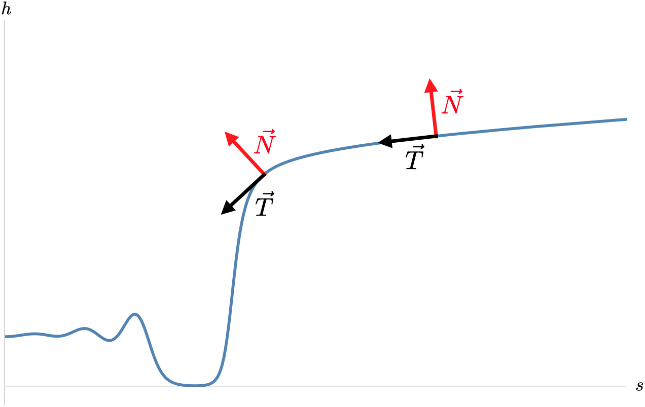
Figure 1: Tangent and normal vectors $\vec{T}$, $\vec{N}$ in field space $(s,h)$.

Projection of the equations of motion to the tangent vector

$$\ddot{\phi}_{0}+3H\dot{\phi}_{0}+U_{T}=0$$ (3.5)

with $U_{T}\equiv T^{a}U_{a}$. Projections to the normal vector $N^{a}$ gives

$$\frac{DT^{a}}{dt}=-\frac{U_{N}}{\dot{\phi}_{0}}N^{a}.$$ (3.6)

We now define the slow-roll parameters by generalizing the setup to a multifield scenario. They take the form

$$\epsilon\equiv-\frac{\dot{H}}{H^{2}}=\frac{\dot{\phi}_{0}^{2}}{2H^{2}}\,\,,\,\,\,\,\eta^{a}\equiv-\frac{1}{H\dot{\phi}_{0}}D_{t}\dot{\phi}^{a}.$$ (3.7)

Note that, the $\eta^{a}$ parameter is now a vector in the sense that there are two degrees in the field space. The same decomposition to $T^{a}$ and $N^{a}$ can be performed to this parameter as well, leading to

$$\eta^{a}=\eta_{\parallel}T^{a}+\eta_{\perp}N^{a}$$ (3.8)

with

$$\eta_{\parallel}\equiv-\frac{\ddot{\phi}_{0}}{H\dot{\phi}_{0}}\,\,,\,\,\,\,\eta_{\perp}\equiv\frac{U_{N}}{\dot{\phi}_{0}H}.$$ (3.9)

Given that $\eta_{\parallel}$ is along the tangential direction of the trajectory, it can be regarded as the extension to the normal $\eta$ slow roll parameter in single field inflation. $\eta_{\perp}$ on the other hand, can also be inserted into eq. (3.6) in the sense that

$$\frac{DT^{a}}{dt}=-H\eta_{\perp}N^{a}\equiv-\dot{\theta}N^{a}$$ (3.10)

hence, the $\eta_{\perp}$ parameter precisely shows how quickly the tangential direction $T^{a}$ is varying in time. The two parameters are related as $\dot{\theta}\equiv H\eta_{\perp}$.

4 Cosmological perturbations

Having the background evolutions, we now perturb the action and describe the scalar perturbations of the model. The notations used are based on [132, 133] (see also [134, 135, 136, 137, 138]).

The fields $\phi^{a}$ and the metric can be perturbed as

$$\phi^{a}(t,\vec{x}) =\phi_{0}^{a}(t)+\delta\phi^{a}(t,\vec{x}),$$ (4.1)

$$ds^{2} =-(1+2\psi)dt^{2}+a(t)^{2}(1-2\psi)\delta_{ij}dx^{i}dx^{j}.$$ (4.2)

Implementing the basis $T^{a}$ and $N^{a}$ to the perturbations allows the following gauge invariant fields

$$v_{T} =aT_{a}\delta\phi^{a}+a\frac{\dot{\phi}_{0}}{H}\psi\equiv aT_{a}Q^{a}$$ (4.3)

$$v_{N} =aN_{a}\delta\phi^{a}\equiv aN_{a}Q^{a}$$ (4.4)

with $Q^{a}\equiv\delta\phi^{a}+\frac{\dot{\phi}^{a}}{H}\psi$ being the Mukhanov-Sasaki variable. In terms of these variables we also define the comoving curvature/isocurvature perturbation

$$\mathcal{R}=\frac{H}{a\dot{\phi}_{0}}v_{T}\equiv\frac{H}{\dot{\phi}_{0}}Q_{T}$$ (4.5)

$$\mathcal{S}=\frac{H}{a\dot{\phi}_{0}}v_{N}\equiv\frac{H}{\dot{\phi}_{0}}Q_{N}.$$ (4.6)

The perturbed action up to second order is then

$$S^{(2)}=\frac{1}{2}\int d^{4}xa^{3}\left[\frac{\dot{\phi}_{0}^{2}}{H^{2}}\dot{\mathcal{R}}^{2}-\frac{\dot{\phi}_{0}^{2}}{H^{2}}\frac{(\nabla\mathcal{R})^{2}}{a^{2}}+{\dot{Q}_{N}}^{2}-\frac{(\nabla Q_{N})^{2}}{a^{2}}+4\dot{\phi}_{0}\eta_{\perp}\dot{\mathcal{R}}Q_{N}-M_{\text{eff}}^{2}Q_{N}^{2}\right]$$ (4.7)

where $M_{\text{eff}}^{2}$ is

$$M_{\text{eff}}^{2}=U_{NN}+H^{2}\epsilon\mathbb{R}-\dot{\theta}^{2}.$$ (4.8)

The equations of motion are

$$\ddot{\mathcal{R}}+\left(3+2\epsilon-2\eta_{\parallel}\right)H\dot{\mathcal{R}}+\frac{k^{2}}{a^{2}}\mathcal{R}=-2\frac{H^{2}}{\dot{\phi}_{0}}\eta_{\perp}\left[\dot{Q}_{N}+\left(3-\eta_{\parallel}+\frac{\dot{\eta}_{\perp}}{H\eta_{\perp}}\right)HQ_{N}\right]$$ (4.9)

$$\ddot{Q}_{N}+3H\dot{Q}_{N}+\left(\frac{k^{2}}{a^{2}}+M_{\text{eff}}^{2}\right)Q_{N}=2\dot{\phi}_{0}\eta_{\perp}\dot{\mathcal{R}}.$$ (4.10)

Both eq. (4.9) and eq. (4.10) incorporate mixing between $\mathcal{R}$ and $Q_{N}$, with the mixing proportional to $\eta_{\perp}$. A naive estimation yields when $\eta_{\perp}\mathrel{\hbox to0.0pt{\lower 4.0pt\hbox{\hskip 1.0pt$\sim$}\hss}\raise 1.0pt\hbox{$>$}}1\rightarrow\dot{\theta}\mathrel{\hbox to0.0pt{\lower 4.0pt\hbox{\hskip 1.0pt$\sim$}\hss}\raise 1.0pt\hbox{$>$}}H$, mixing between the two perturbations become significant and $Q_{N}$ can source $\mathcal{R}$.

In addition to the mixing, eq. (4.8) incorporates the essentials that determine the dynamics of $Q_{N}$. $M_{\text{eff}}^{2}$ can take a negative value either through 1) $U_{NN}<0$, 2) $\mathbb{R}<0$, corresponding to a hyperbolic geometry in the field space, 3) $\dot{\theta}^{2}>U_{NN}$. In any case, a tachyonic isocurvature mass then modifies the equations of motion for $k^{2}/a^{2}<|M_{\text{eff}}^{2}|$ to be

$$\ddot{Q}_{N}+3H\dot{Q}_{N}-\left(\left|M_{\text{eff}}^{2}\right|\right)Q_{N}\simeq 0.$$ (4.11)

Hence $Q_{N}$ can exhibit an exponential growth due to the tachyonic mass. This growth can be more rapid than cases implementing a USR phase.

5 Inflaton and perturbation evolution

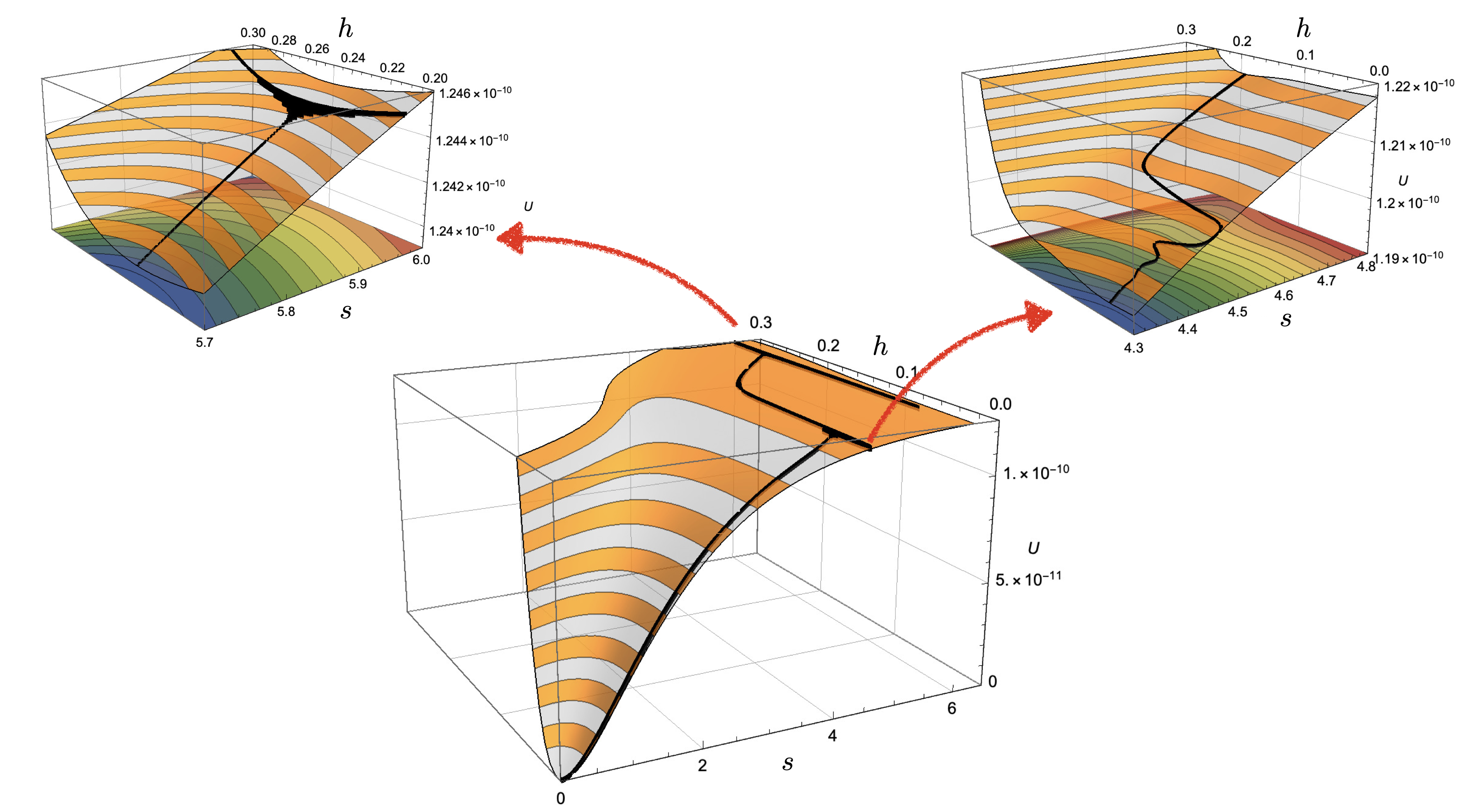
Figure 2: Potential and field trajectory (black) of the setup. Note that the inflaton follows a well defined valley with a positive $M_{\text{eff}}^{2}$, allowing the trajectory to be independent to the initial conditions (top-left). The potential then exhibits a region where the valley disappears, inducing a turn in the trajectory and approaches the hill (top-right). After evolving along this tachyonic hill, the inflaton falls back down into a valley.

We now turn our interest to the dynamics in the critical Higgs-$R^{2}$ setup, starting with the trajectory, which is schematically depicted in figure 2.

• Stage 1: Initially the inflaton starts rolling down a well defined valley, satisfying the slow-roll conditions. The large and positive $M_{\text{eff}}^{2}$ ensures the isocurvature perturbation $Q_{N}$ be suppressed. This initial valley allows the large scale predictions (e.g. CMB) to be insensitive to the initial values of the inflaton, simply speaking it exhibits an attractor prediction.

• Stage 2: Then the inflaton rolls down in the Higgs direction, approaching the hill at $h=0$.

• Stage 3: Once the inflaton climbs up the hill where $h\approx 0$, the inflaton exhibits a turn, and now evolves in the $s$ direction. The isocurvature mass $M_{\text{eff}}^{2}$ becomes large and negative, with its value mainly determined by $\xi$. Its precise value takes the form

  $$M_{\text{eff}}^{2}\simeq\frac{1}{\dot{s}^{2}+e^{-\sqrt{\frac{2}{3}}{s}}\dot{h}^{2}}\left(e^{\sqrt{\frac{2}{3}}{s}}\dot{s}^{2}\frac{\partial^{2}U}{\partial h^{2}}\right)\simeq-3M^{2}\left[\xi_{0}+b_{\xi}\ln\left(\frac{h}{h_{m}}\right)+\frac{9}{2}b_{\xi}\right]\left(1-e^{-\sqrt{\frac{2}{3}}{s}}\right).$$ (5.1)

  The inflaton then exhibits another turn back into the valley.

• Stage 4: The inflaton once again rolls into the well defined valley, with a large and positive $M_{\text{eff}}^{2}$.

Let’s look into Stage 1, 2, 3 in more detail.

5.1 Stage 1.

In this region, where $M_{\text{eff}}^{2}>H^{2}>0$ and the turn rate $\dot{\theta}\ll H$, the equations of motion simply resemble standard effective single field, slow-roll results. The equations take the form, with the transformation of the time variable to efolds using $N_{e}=\int^{t}dt^{\prime}H(t^{\prime})$

$$\frac{d^{2}\mathcal{R}_{k}}{dN_{e}^{2}}+\left(3+\epsilon-2\eta_{\parallel}\right)\frac{d{\mathcal{R}_{k}}}{dN_{e}}+\frac{k^{2}}{a^{2}H^{2}}\mathcal{R} =0$$ (5.2)

$$\frac{d^{2}{Q}_{N,k}}{dN_{e}^{2}}+3\frac{d{Q}_{N,k}}{dN_{e}}+\left(\frac{k^{2}}{a^{2}H^{2}}+\frac{M_{\text{eff}}^{2}}{H^{2}}\right)Q_{N,k} =0$$ (5.3)

which, neglecting the slow-roll parameters as they are suppressed, give the generally known solutions with ${\epsilon_{k}^{2}\equiv k^{2}/a^{2}H^{2}}$ [122, 123]

$$\mathcal{R}_{k}(N_{e}) =e^{-\frac{3}{2}N_{e}}\left[c_{1}\,e^{-\frac{N_{e}}{2}\sqrt{9-4\epsilon_{k}^{2}}}+c_{2}\,e^{\frac{N_{e}}{2}\sqrt{9-4\epsilon_{k}^{2}}}\right]$$ (5.4)

$${Q}_{N,k}(N_{e}) =e^{-\frac{3}{2}N_{e}}\left[c_{3}\,e^{-\frac{N_{e}}{2}\sqrt{9-4\frac{M_{\text{eff}}^{2}}{H^{2}}-4\epsilon_{k}^{2}}}+c_{4}\,e^{\frac{N_{e}}{2}\sqrt{9-4\frac{M_{\text{eff}}^{2}}{H^{2}}-4\epsilon_{k}^{2}}}\right]$$ (5.5)

where $c_{1},\,c_{2},\,c_{3},\,c_{4}$ are determined by the conditions at the in-horizon state. We can see that for the case when $\epsilon_{k}^{2}\ll 1$, i.e. out of the horizon, $\mathcal{R}_{k}(N_{e})\propto\mathcal{R}_{0}+\mathcal{R}_{1}e^{-3N_{e}}$ and has a mode freezing out, being constant deep outside the horizon. The isocurvature mode $Q_{N,k}$, in contrast, always is suppressed as $Q_{N,k}(N_{e})\propto e^{-\frac{3}{2}N_{e}}e^{\pm i\frac{M_{\text{eff}}}{H}N_{e}}$ due to $M_{\text{eff}}\gg H$ in this regime, and therefore is exponentially suppressed in the deep out of horizon region, giving negligible effects on cosmological observables.

We now obtain standard effective single field slow-roll observables. As the inflaton evolution in this era remains in the same $h$ order, we approximate $\xi(h)\simeq\xi_{0}$. In this period, the fields resemble the approximate relation in the large-scale observable region

$$s_{v}\approx\sqrt{\frac{3}{2}}\ln\left[1+\frac{4(\lambda_{m}+3M^{2}\xi_{0}^{2})h^{2}+(7h-5h_{m})(h-h_{m})b}{12M^{2}\xi_{0}}\right]$$ (5.6)

allowing us to combine the fields to be parameterized with the scalaron only, leading to the slow roll parameters

$$\epsilon_{H}\simeq\epsilon_{V}\equiv\frac{1}{2}\left.\left[\frac{U_{s}(s,h(s))}{U(s,h(s))}\right]^{2}\right|_{s=s_{*}}\,\,,\,\,\,\,\,\eta_{\parallel}\simeq\eta_{V}\equiv\left.\frac{U_{ss}(s,h(s))}{U(s,h(s))}\right|_{s=s_{*}}$$ (5.7)

with $s_{*}$ being the scalaron field value at the CMB pivot scale and

$$n_{s}\equiv 1+\frac{d\ln{\mathcal{P}_{\mathcal{R}}(k)}}{d\ln k}\simeq 1-6\epsilon_{V}+2\eta_{V}\,\,,\,\,\,\,\,r\simeq 16\epsilon_{V}.$$ (5.8)

The inflationary epoch exhibits slow-roll with $\eta_{H}\ll 1$, and the $\frac{\lambda(h)}{4}h^{4}$ term in the potential eq. 2.4 is orders smaller than other terms. This lets us reasonally take the inflationary efolds $N_{\text{inf}}=N_{\text{end}}-N_{\text{pivot}}\approx\frac{3}{4}e^{\sqrt{\frac{2}{3}}s_{*}}$, which resembles an $R^{2}$ inflation-like form. Therefore, the above expressions can be approximately expressed to

$$n_{s}\approx \,\,1-\frac{2}{N_{\text{inf}}}-\frac{9}{2N_{\text{inf}}^{2}}$$ (5.9)

$$+\frac{M^{2}\xi_{0}^{2}\,b}{\lambda_{m}\left(\lambda_{m}+3M^{2}\xi_{0}^{2}\right)}\left[2+\frac{3\left(2+3\ln\left(\frac{(\lambda_{m}+3M^{2}\xi_{0}^{2})h_{m}^{2}}{4M^{2}\xi_{0}N_{\text{inf}}}\right)\right)}{2N_{\text{inf}}}+\frac{27\left(1+\ln\left(\frac{(\lambda_{m}+3M^{2}\xi_{0}^{2})h_{m}^{2}}{4M^{2}\xi_{0}N_{\text{inf}}}\right)\right)}{4N_{\text{inf}}^{2}}\right]$$

and

where $N_{\text{end}}$ describes the efolds at the end of inflation, and $N_{\text{pivot}}$ represents the efolds at the CMB pivot scale. Therefore the additional logarithmic running of the Higgs self coupling shifts the spectral index of the curvature power spectrum to larger values compared to the pure Higgs-$R^{2}$ case with a constant Higgs self coupling.

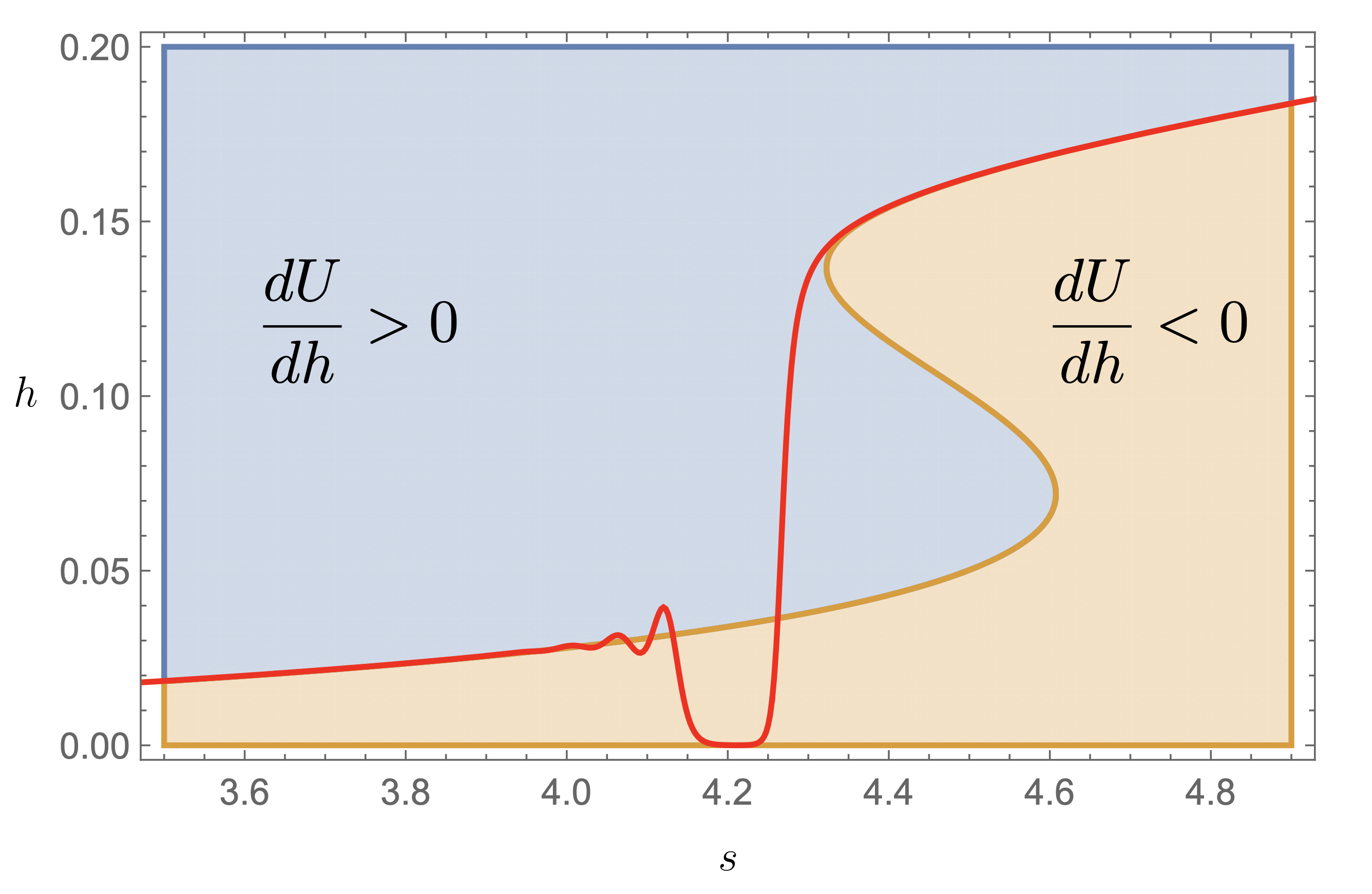
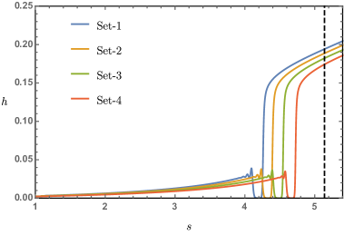
Figure 3: (Left) Contour of $\frac{dU}{dh}=0$, with the trajectory of the inflaton colored in red. Once $h$ reaches $h_{local\,\,min}$, $\frac{dU}{dh}>0$, making the inflaton fall down towards the hill. (Right) Trajectory for several parameter sets, where the dashed black line expresses the field value for $N_{\text{inf}}=50$. The position where hill-climbing occurs depends on $\xi$ values.

5.2 Stage 2.

This stage contains the initial deviation from the valley. Recall that for the Higgs-$R^{2}$ potential, the inflaton initially follows a valley well defined by $\partial_{h}U=0$, in which the scalaron field at the valley $s_{v}$ takes the expression

$$s_{v}\simeq\sqrt{\frac{3}{2}}\ln\left[\frac{6M^{2}\xi_{0}+2h^{2}\left(\lambda_{m}+3M^{2}\xi_{0}^{2}\right)+b\,h^{2}\ln\left(\frac{h}{h_{m}}\right)\left(2\ln\left(\frac{h}{h_{m}}\right)+1\right)}{6M^{2}\xi_{0}}\right].$$ (5.11)

This trajectory in general, can have critical points in the $(h,s)$ plane, being

$$\frac{h_{local\,\,max}}{h_{m}}\simeq e^{-\frac{3}{4}-\frac{\sqrt{5b^{2}-16b\lambda_{m}-48bM^{2}\xi_{0}^{2}}}{4b}}\,\,,\,\,\,\frac{h_{local\,\,min}}{h_{m}}\simeq e^{-\frac{3}{4}+\frac{\sqrt{5b^{2}-16b\lambda_{m}-48bM^{2}\xi_{0}^{2}}}{4b}}.$$ (5.12)

Note that these extremal points in the field space exist when the following conditions are satisfied

$$0\leq\xi_{0}\lesssim\frac{1}{4\sqrt{3}M}\sqrt{5b-16\lambda_{m}}\,\,,\,\,\,\lambda_{m}<\frac{5b}{16}.$$ (5.13)

We focus on the trajectory point $h_{local\,\,min}$. Once the inflaton hits this point, $\partial_{h}U>0$ in the order

$$\left.\frac{\partial U}{\partial h}\right|_{s_{v}(h_{local\,\,min}),\,h_{local\,\,min}\pm\delta}=A\,\delta^{2}+\mathcal{O}(\delta^{3})$$ (5.14)

for both $h_{local\,\,min}+\delta$ and $h_{local\,\,min}-\delta$ with $\delta>0$, with $A$ being a positive constant. Therefore, the inflaton starts rolling down towards the $h$ direction, approaching the hill at $h=0$. This is depicted in figure 3. where the figure focuses on the transition region, and it shows that the potential exhibits a region where $dU/dh>0$ giving a roll-down towards the hill.

5.3 Stage 3.

This stage is precisely where the large and negative isocurvature mass induces an exponential growth in the isocurvature perturbation $Q_{N}$. The evolution of the perturbations are depicted in figure 4.

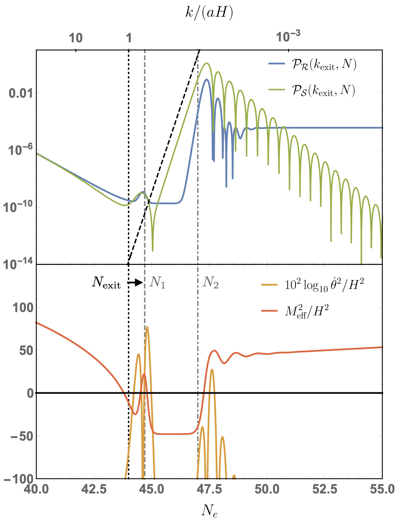
Figure 4: (Top) Perturbation evolution for the $k$ mode that exits the horizon at $N_{\text{exit}}=44$. The efolds when the inflaton starts and stops rolling down the hill are denoted as $N_{1}$ and $N_{2}$ respectively. The black-dashed line represents the growth $\mathcal{P}_{\mathcal{S}}\propto\exp\left[\left(\frac{2|M_{\text{eff}}|}{H}-3\right)N_{e}\right]$. (Bottom) $M_{\text{eff}}^{2}/H^{2}$ and $\dot{\theta}^{2}/H^{2}$ evolution. The tachyonic $M_{\text{eff}}$ induces an exponential growth in the $\mathcal{P}_{\mathcal{S}}$, and due to the mixing between curvature and isocurvature perturbations this enhancement is translated over to $\mathcal{P}_{\mathcal{R}}$.

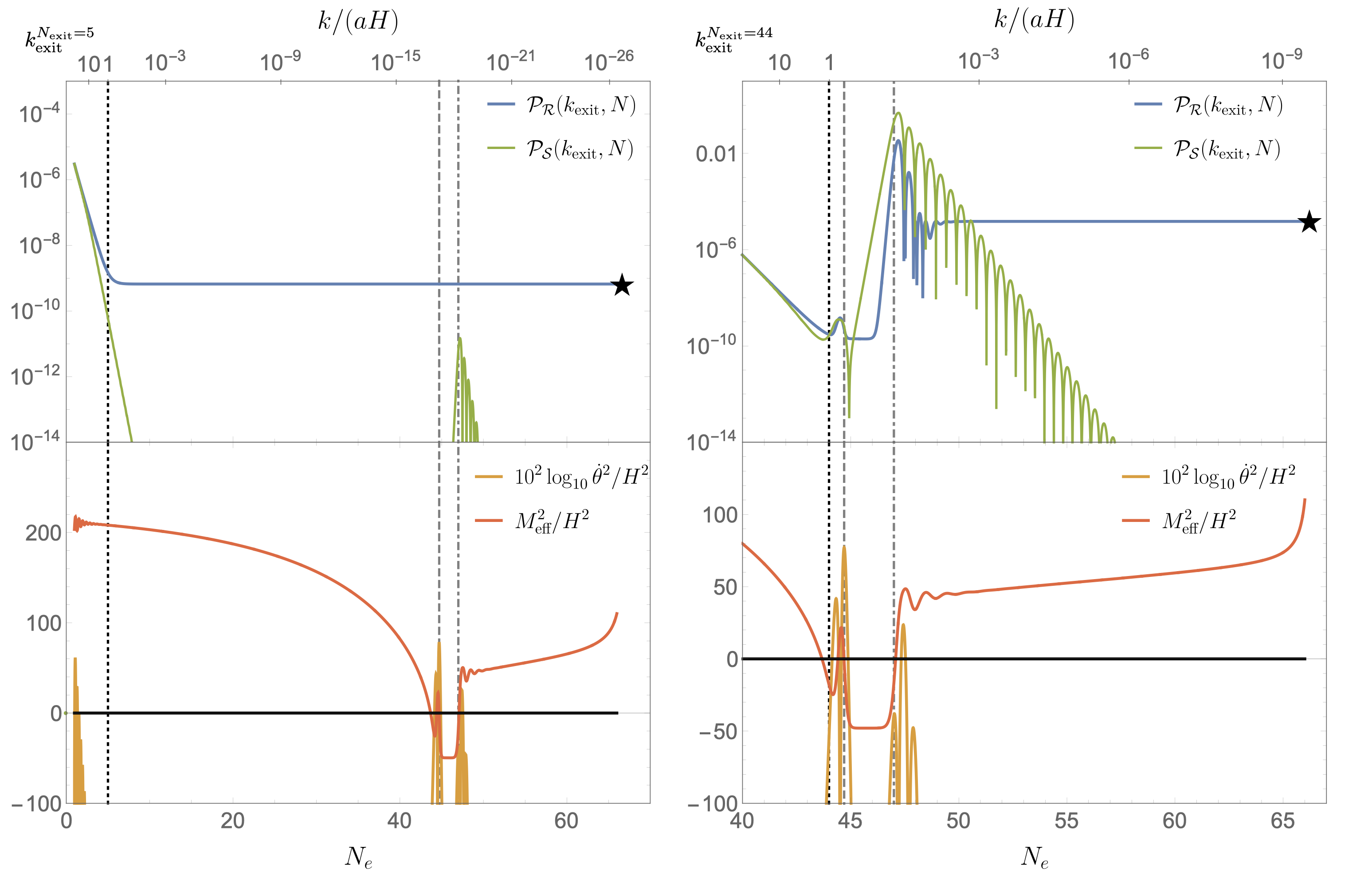
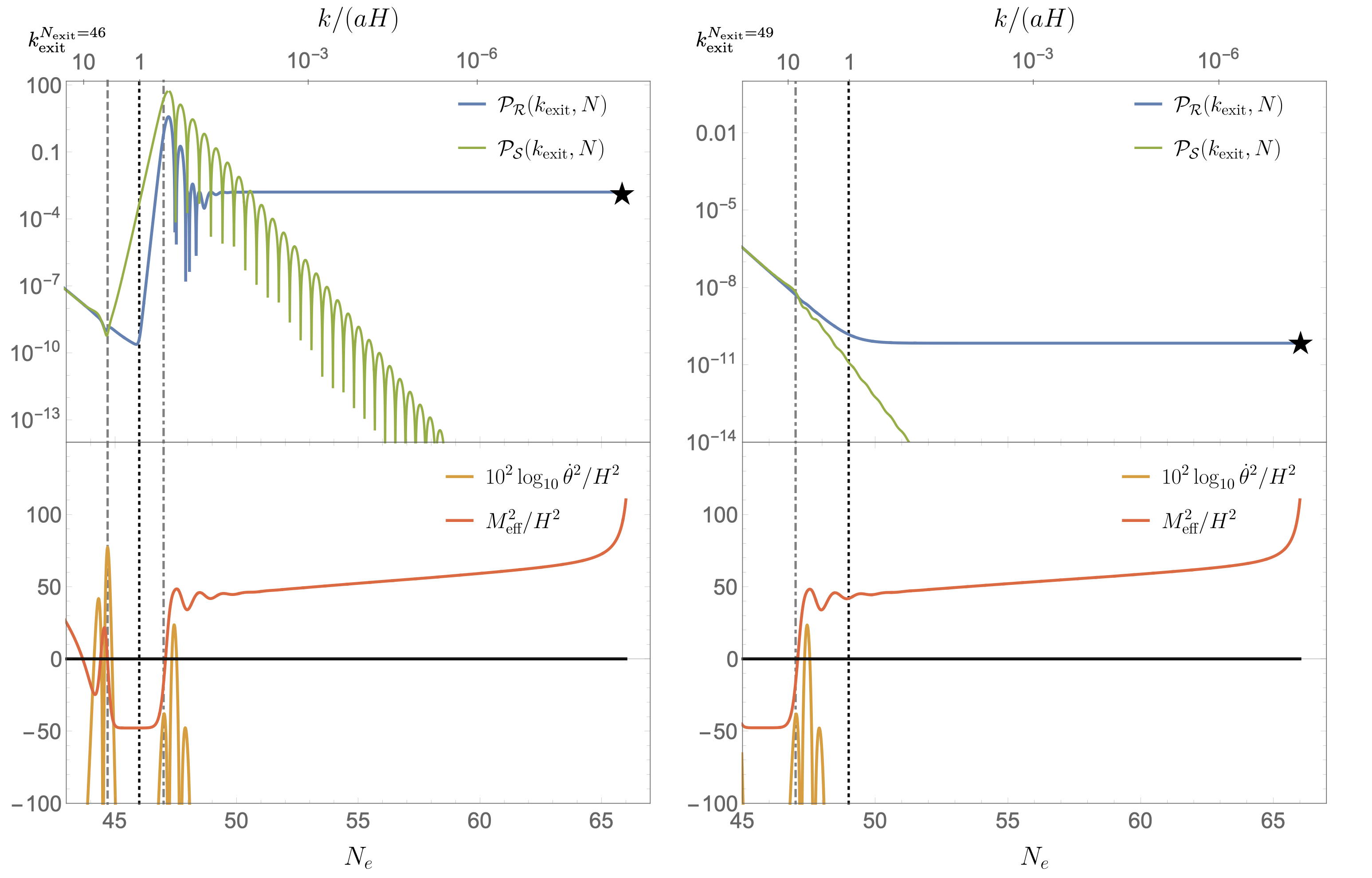
Figure 5: Compilation of the perturbations for $k_{\text{exit}}$ leaving at certain scales, which corresponds to a definite $N_{\text{exit}}$. We observe that after the tachyonic increase of the isocurvature, and consequentially the curvature perturbation, the isocurvature part exponentially decays, and the perturbations become adiabatic at scales evaluated at the end of inflation ($N_{\text{end}}$ in the plot, shown at the star).

From the first turn, due to the mixing term in the equations of motion, the perturbations mix and as $\dot{\theta}^{2}/H^{2}>1$, the $\mathcal{R}$ experiences a slight bump in its evolution, however its effect is negligible.

The period when the inflaton rolls down the hill, where the starting efolds at $N_{1}$ and the end efolds at $N_{2}$, the isocurvature mass takes $M_{\text{eff}}^{2}/H^{2}\ll 0$, therefore the isocurvature perturbation $Q_{N}$ is dominated by the exponential growth from the negative isocurvature mass. Recalling the isocurvature perturbations equations eq. (4.10), eq. (5.3) while neglecting the source terms ,as this is precisely the case when the inflaton rolls down the $h=0$ hill,

$$\frac{d^{2}{Q}_{N,k}}{dN_{e}^{2}}+3\frac{d{Q}_{N,k}}{dN_{e}}+\left(\frac{k^{2}}{a^{2}H^{2}}-\frac{|M_{\text{eff}}^{2}|}{H^{2}}\right)Q_{N,k}=0$$ (5.15)

with the solutions

$${Q}_{N,k}(N_{e})=e^{-\frac{3}{2}N_{e}}\left[d_{3}\,e^{-\frac{N_{e}}{2}\sqrt{9-4\frac{M_{\text{eff}}^{2}}{H^{2}}-4\epsilon_{k}^{2}}}+d_{4}\,e^{\frac{N_{e}}{2}\sqrt{9-4\frac{M_{\text{eff}}^{2}}{H^{2}}-4\epsilon_{k}^{2}}}\right]\xrightarrow[|M_{\text{eff}}^{2}|\gg H^{2}]{\epsilon_{k}^{2}\ll 1}d_{4}~{}e^{\left(\frac{|M_{\text{eff}}|}{H}-\frac{3}{2}\right)N_{e}}$$ (5.16)

with the $M_{\text{eff}}^{2}$ in this period taking the form of eq. (5.1). Consequentially,

$$\mathcal{P}_{\mathcal{S}}(k_{\text{exit}},N_{e})=\frac{k_{\text{exit}}^{3}}{2\pi^{2}}\frac{H^{2}}{\dot{\phi}_{0}^{2}}\langle Q_{N,k}\,Q_{N,k}\rangle=\mathcal{P}_{\mathcal{S}}(k_{\text{exit}},N_{1})~{}e^{\left(\frac{2|M_{\text{eff}}|}{H}-{3}\right)(N_{e}-N_{1})}$$ (5.17)

therefore $Q_{N,k}$, and consequentially $\mathcal{P}_{\mathcal{S}}$ grows exponentially during this period. $\mathcal{R}$, however, does not grow instantaneously, precisely due to the fact that $\dot{\theta}^{2}/H^{2}\ll 1$ in this period. Then, as the second turn with $\dot{\theta}^{2}/H^{2}\gg 1$ occurs, the enhanced $Q_{N}$ is then sourced to $\mathcal{R}$, now also exponentially growing and decaying according to the mixing, will then stop evolving in the superhorizon limit when $\dot{\theta}^{2}/H^{2}\ll 1$ occurs again.

One may raise the following question:is eq. (2.9) a sufficient approximation for this scenario, judging by the fact that $h$ approaches 0. The answer is yes. The turn in the trajectory occurs around eq. (5.12) where $h_{local\,\,min}\sim h_{m}$. The region where $h\ll h_{m}$, the potential term $U\supset\frac{\lambda(h)}{4}h^{4}e^{-2\sqrt{\frac{2}{3}}s}$ is subdominant.

6 Power spectrum and PBH abundance

We numerically compute the cosmological perturbations in this scenario using PyTransport [139]. Here we present several parameter sets exhibiting this large local feature in the power spectrum, enlisted in Table 1. The Planck CMB pivot scale is set as $k_{*}=0.05~{}\text{Mpc}^{-1}$.

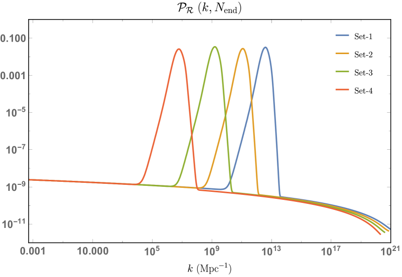
Figure 6: The observational curvature power spectrum $\mathcal{P}_{\mathcal{R}}(k,N_{\text{end}})$ for the benchmark parameter sets in Table 1.

Set	$M(M_{P})$	$\xi_{0}$	$\lambda_{m}(\times 10^{-6})$	$\beta_{2}$	$\beta_{\xi}^{0}$	$h_{m}\,(M_{P})$	$k_{max}\,(\text{Mpc}^{-1})$	$\mathcal{P}_{\mathcal{R},max}$	$n_{s}$	$r$
$1$	$1.3\times 10^{-5}$	$4.0$	$4.1743336$	$0.5$	$-0.01$	$0.21$	$3.9\times 10^{12}$	$0.032$	$0.967$	$0.004$
$2$	$1.3\times 10^{-5}$	$3.5$	$4.1003376$	$0.5$	$-0.01$	$0.21$	$1.2\times 10^{11}$	$0.027$	$0.967$	$0.004$
$3$	$1.3\times 10^{-5}$	$3.0$	$4.0109148$	$0.5$	$-0.01$	$0.21$	$1.6\times 10^{9}$	$0.034$	$0.967$	$0.004$
$4$	$1.3\times 10^{-5}$	$2.5$	$3.8998765$	$0.5$	$-0.01$	$0.21$	$6.5\times 10^{6}$	$0.02$	$0.967$	$0.004$

Table 1: Several benchmark parameter sets ($M$, $\xi_{0}$, $\lambda_{m}$, $\beta_{2}=(4\pi)^{4}\,b$, $\beta_{\xi}^{0}=b_{\xi}/2$, $h_{m}$) and their corresponding small-scale observables.

The corresponding curvature power spectrum $\mathcal{P}_{\mathcal{R}}(k)$ for these parameter sets are depicted in figure 6. Each exhibit a near-scale invariant power spectrum with $n_{s}$ giving perfect consistency with current Planck CMB observations [140, 141]. Note that the CMB predictions also are consistent among parameters, regardless of the position of the localized peak. This is precisely due to the fact that the tachyonic enhancement of the curvature/isocurvature perturbations induces an exponential increase, requiring a much shorter period on how long this instability sustains. This amplified $\mathcal{P}_{\mathcal{R}}$ at small scales can also lead to copious PBH production, which depending on the mass of the PBH can account for the majority of the dark matter in our universe. Taking a peaks theory approach [142, 143, 144, 145, 146, 147, 148, 149], where the details are in Appendix A., we depict the PBH abundance $f_{\text{PBH}}(M_{\text{PBH}})=\Omega_{\text{PBH}}/\Omega_{\text{DM}}$ in figure 7., taking a common critical density contrast $\delta_{c}=0.41$ [150, 151] and a Gaussian window function $W(k,R)=\exp\left(-\frac{k^{2}R^{2}}{2}\right)$. One major feature the tachyonic instability-induced $\mathcal{P}_{\mathcal{R}}$ enhancement composes is that it can cover all viable mass ranges of PBHs, which is in contrast with our previous USR induced PBH studies [53].

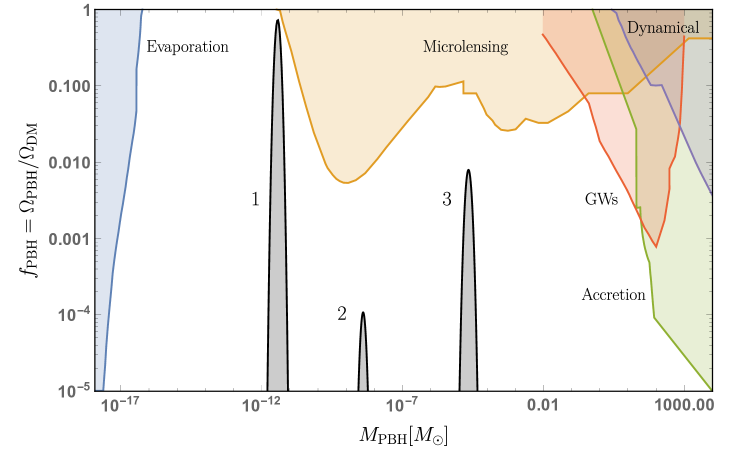
Figure 7: The corresponding PBH abundances for the benchmark parameter sets in Table 1. The observational constraints are taken from [79, 152]. Depending on the parameters the tachyonic instability-induced perturbations one can induce scenarios where PBHs can consist a significant amount of dark matter within the constraint bounds. Set-4 is not depicted in the figure range due to a smaller peak value $\mathcal{P}_{\mathcal{R},max}$.

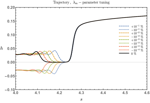
Figure 8: Parameter sensitivity on the inflaton trajectory. For demonstration, we take the parameter $\lambda_{m}$ tuning for Set. 1 in Table 1. The percentage level corresponds to the parameter $\delta\lambda_{m}/\lambda_{m}$.

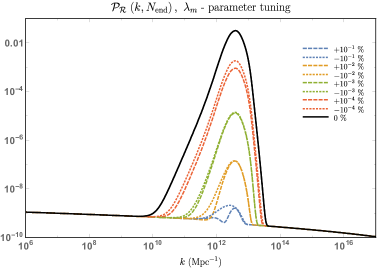
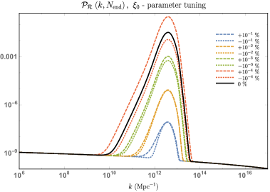
Figure 9: (Left )The degree of parameter $\lambda_{m}$ tuning for Set. 1 in Table 1. The percentage level corresponds to the parameter $\delta\lambda_{m}/\lambda_{m}$. (Right) The degree of parameter $\xi_{0}$ tuning for Set. 1 in Table 1. The percentage level corresponds to the parameter $\delta\xi_{0}/\xi_{0}$.

6.1 Degree of parameter tuning

Obviously, the tachyonic enhancement is subject to parameter tuning. The evolution of the inflaton along the hill determines the amount of enhancement, and as this period itself is unstable the parameters will need some degree of tuning to have a noticeable perturbation growth.

To show this, we choose the Set 1. parameters and vary $\lambda_{m}$ and $\xi_{0}$ and explicitly allowing the $h<0$ region. As depicted in figure 8., the field evolution along the $h=0$ hill is sensitive to the parameter choices. This difference to the evolution period on the hill leads to a difference in the curvature power spectrum peak, depicted in figure 9. Notice that in order to sustain an enhancement in the curvature power spectrum to be $\mathcal{P}_{\mathcal{R}}\sim 10^{-2}$, the parameter $\delta\lambda_{m}/\lambda_{m}\equiv(\lambda_{m}^{dev}-\lambda_{m})/\lambda_{m}\sim\mathcal{O}(10^{-4})\,\%$, with $\lambda_{m}^{dev}$ being the parameter that deviates from the benchmark set parameter, which is in similar orders with fine-tuning degrees in single-field polynomial inflation models as well [39]. The $\xi_{0}$ parameter, on the other hand, is an order less sensitive to achieve the same order of enhancement, with $\delta\xi_{0}/\xi_{0}\equiv(\xi_{0}^{dev}-\xi_{0})/\xi_{0}\sim\mathcal{O}(10^{-3})\,\%$, Noticeably, if one requires the detectability of the SGWB, the required enhancement softens to $\mathcal{P}_{\mathcal{R}}\sim 10^{-4}\,(10^{-5})$, hence the tuning of the parameters also decrease to an order less to be $\delta\lambda_{m}/\lambda_{m}\sim\mathcal{O}(10^{-3})\,\%$, $\delta\xi_{0}/\xi_{0}\sim\mathcal{O}(10^{-2})\,\%$.

7 Stochastic gravitational wave background (SGWB) at the second order

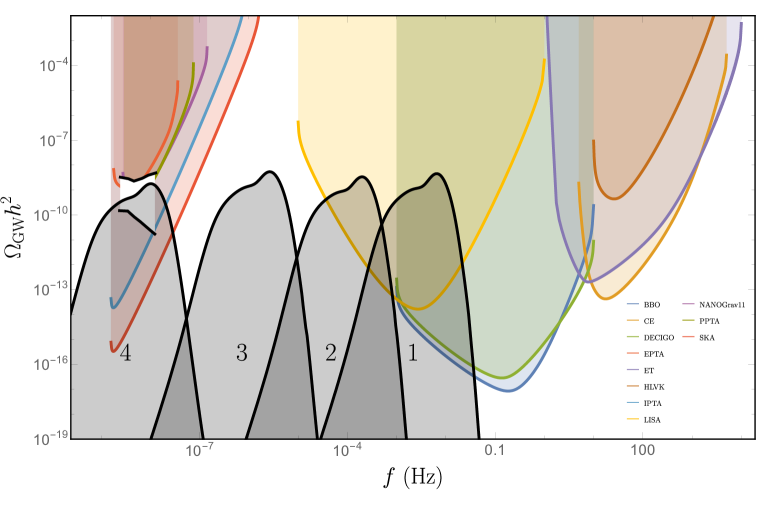
Figure 10: The corresponding GW abundances for the benchmark parameter sets in Table 1, overlayed over various gravitational wave observatory’s sensitivity curves [153, 154]. The white region at nano-Hertz frequency corresponds to the NANOGrav 12.5 year results [3].

The amplified curvature perturbations also lead to a copious amount of stochastic GWs. The current energy density fraction per logarithmic wavelength of the GWs from second order is, following [155, 156]

$$\Omega_{\text{GW}}(\eta_{0},k)=c_{g}\frac{\Omega_{r,0}}{6}\int_{0}^{\infty}dv\int_{|1-v|}^{1+v}du\left(\frac{4v^{2}-(1+v^{2}-u^{2})^{2}}{4uv}\right)^{2}\overline{\mathcal{I}^{2}(v,u)}\mathcal{P}_{\mathcal{R}}(kv)\mathcal{P}_{\mathcal{R}}(ku)$$ (7.1)

where $\Omega_{r,0}\approx 5.38\times 10^{-5}$ is the current radiation energy density fraction [140], $x\equiv k\eta$ with $\eta$ being the conformal time, $c_{g}\equiv\frac{a_{f}^{4}\rho_{r}(\eta_{f})}{\rho_{r}(\eta_{0})}=\frac{g_{*}}{g_{*}^{0}}\left(\frac{{g_{*}^{0}}_{S}}{{g_{*}}_{S}}\right)^{4/3}\approx 0.4$ by taking the current universe effective energy and entropy degree of freedom as $g_{*}^{0}=3.36$ and ${g_{*}^{0}}_{S}=3.91$ respectively. The degree of freedom at the evaluation of perturbations take the value ${g_{*}}={g_{*}}_{S}=106.75$. $\overline{\mathcal{I}^{2}(v,u)}$ is expressed analytically in radiation-domination as [155, 156, 157].

$$\overline{\mathcal{I}^{2}(v,u)}=\frac{1}{2}\left[\frac{3(u^{2}+v^{2}-3)}{4u^{3}v^{3}}\right]^{2} \left[\left(-4uv+(u^{2}+v^{2}-3)\ln\left|\frac{3-(u+v)^{2}}{3-(u-v)^{2}}\right|\right)^{2}\right.$$

$$+\left.\pi^{2}(u^{2}+v^{2}-3)^{2}\Theta(v+u-\sqrt{3})\right].$$ (7.2)

The current universe SGWB energy fraction $\Omega_{\text{GW}}\,h^{2}$ for our benchmark parameters are depicted in figure 10. Note that due to the nature of the tachyonic instability, the GW spectrum can span over all frequencies from aLIGO frequencies all the way up to PTA frequencies. Utilizing current and future GW observatories, we can obtain useful information on the $\xi$ and $\lambda(h)$ parameters, ultimately gaining information on the running behavior of the SM Higgs self coupling for high energy scales. Noticeably, our Set. 4 parameters directly correspond to the recently reported NANOGrav results. Therefore, these running parameters and nonminimal coupling values, if the results are confirmed to be indeed a SGWB, will be able to be a possible source of the observed SGWB.

8 Conclusion and Discussions

In this work we demonstrated that the $\lambda$ running in Higgs-$R^{2}$ inflation can be implemented in the effective production of enhanced curvature perturbations, consequentially leading to amplified second order stochastic gravitational wave productions and possibly primordial black holes. The two field potential characterized by the scalaron and Higgs $(s,h)$ exhibits a temporary valley structure breakdown induced by the running of $\lambda(h)$. The inflaton then rolls down towards the hill at $h=0$, where there is a tachyonic instability that depends on the scalaron mass $M$ and the nonminimal coupling $\xi$. Isocurvature perturbations are exponentially enhanced, which are transferred to the curvature perturbation as the inflaton rolls back down the hill and settles at the lower field valley. Compared to our previous work that implemented a ultra-slow-roll phase [53], the tachyonic enhancement presented in this work occurs in a much shorter duration, hence allowing for effectively all mass ranges of primordial black hole dark matter without conflicting Planck CMB observables. It also allows parameters that coincide with the recently reported stochastic process by NANOGrav and other PTA observatories.

There are several aspects to foresee from here. In this work we effectively parameterized the $\lambda$ running with the parameters $\lambda_{m},~{}b,~{}h_{m}$. In principle these will correspond to the physical running parameters $m_{top},~{}\alpha_{s},~{}m_{W}$ at low energies, therefore providing a connection between the low energy SM parameters and the inflationary features. A full parameter scan of these SM parameters that incorporate a sizable $\mathcal{P}_{\mathcal{R}}$ at a certain scale will provide information on the running parameters of our Standard Model Higgs, which we seek to pursue in a future work [158].

Also, in this work we only considered Gaussian fluctuations in the cosmological perturbations. It is well known that multi-field inflation, especially those incorporating a tachyonic instability may exhibit high levels on non-Gaussianity, which will alter the predictions of SGWB, and PBH abundances [159, 160, 161, 162, 163]. We leave the computation of non-Gaussianity and its impact on small scale observables for a future work.

Appendix A Peaks theory approach on the PBH abundance calculation.

In this appendix we address the peaks theory approach to calculate the PBH abundance. The density contrast power spectrum is related to the curvature power spectrum through the following formula

$$\mathcal{P}_{\delta}(k)=\frac{4(1+w)^{2}}{(5+3w)^{2}}\left(\frac{k}{aH}\right)^{4}\mathcal{P}_{\mathcal{R}}(k)\rightarrow\frac{16}{81}\left(\frac{k}{aH}\right)^{4}\mathcal{P}_{\mathcal{R}}(k)\,\,\,\text{ in RD : $w=\frac{1}{3}$ . }$$ (A.1)

We then smooth the density contrast to a typical scale $R=\frac{1}{aH}$, with a window function $W(k,R)$ in Fourier space. Hence, the spectral index of the density contrast with a window function will take the form

$$\sigma_{i}^{2}(R)=\int_{0}^{\infty}\frac{dk}{k}k^{2i}W^{2}(k,R)\mathcal{P}_{\mathcal{\delta}}=\frac{16}{81}\int_{0}^{\infty}\frac{dk}{k}k^{2i}W^{2}(k,R)\mathcal{P}_{\mathcal{R}}$$ (A.2)

with the $i=0$-th moment corresponding to the variance $\sigma_{0}^{2}(R)\equiv\langle\delta^{2}(\mathbf{x},R)\rangle$ . The PBH mass can be expressed as a function to the associated horizon mass

$$M_{\text{PBH}}=\mathcal{K}M_{H}=\frac{\mathcal{K}}{2GH}$$ (A.3)

with $M_{H}$ being the horizon mass, $\mathcal{K}$ being the collapse efficiency. We take $\mathcal{K}=0.2$. Associating the mass with the relevant wave number, we get the following scaling

$$M_{\text{PBH}}=4.64\times 10^{15}~{}{\gamma}\left(\frac{g_{*}}{106.75}\right)^{-\frac{1}{6}}\left(\frac{k_{\text{PBH}}}{k_{*}}\right)^{-2}M_{\odot}$$ (A.4)

with $k_{*}=0.05~{}\text{Mpc}^{-1}$ denoting the CMB pivot scale and $g_{*}=106.75$ the relativistic degrees of freedom at that epoch.

In peaks theory [142] ( see also [143, 144, 145, 146, 147, 148, 149]) , the PBH mass fraction $\beta_{\text{PBH}}(M)\equiv\left.\frac{\rho_{\text{PBH}}(M)}{\rho_{\text{tot}}}\right|_{\text{formation}}$ is related to the peak number density over a criteria $\nu>\nu_{c}$

$$n(\nu_{c})=\frac{1}{(2\pi)^{2}}\left(\frac{\sigma_{2}}{\sqrt{3}\sigma_{1}}\right)^{3}\int_{\nu_{c}}^{\infty}d\nu\int_{0}^{\infty}d\xi_{1}\frac{f(\xi_{1})}{\sqrt{2\pi(1-\gamma^{2})}}\exp{\left[-\frac{1}{2}\left(\nu^{2}+\frac{(\xi_{1}^{2}-\gamma\nu)^{2}}{1-\gamma^{2}}\right)\right]}$$ (A.5)

leading to the relation

$$\beta_{\text{PBH}}(R) =n(\nu_{c})(2\pi)^{3/2}R^{3}$$

$$=\frac{1}{\sqrt{2\pi}}\left(\frac{R\sigma_{2}}{\sqrt{3}\sigma_{1}}\right)^{3}\int_{\nu_{c}}^{\infty}d\nu\int_{0}^{\infty}d\xi_{1}\frac{f(\xi_{1})}{\sqrt{2\pi(1-\gamma^{2})}}\exp{\left[-\frac{1}{2}\left(\nu^{2}+\frac{(\xi_{1}^{2}-\gamma\nu)^{2}}{1-\gamma^{2}}\right)\right]}.$$ (A.6)

The parameters stated here are $\nu=\frac{\delta}{\sigma_{0}}$, $\nu_{c}=\frac{\delta_{c}}{\sigma_{0}}$,$\gamma=\frac{\sigma_{1}^{2}}{\sigma_{0}\sigma_{2}}$, and the $f(\xi_{1})$ function being

$$f(\xi_{1})=\frac{1}{2}(\xi_{1}^{3}- 3\xi_{1})\left(\text{erf}\left[\sqrt{\frac{5}{2}}\xi_{1}\right]+\text{erf}\left[\sqrt{\frac{5}{8}}\xi_{1}\right]\right)$$

$$+\sqrt{\frac{2}{5\pi}}\left\{\left(\frac{8}{5}+\frac{31}{4}\xi_{1}^{2}\right)\exp\left[-\frac{5}{8}\xi_{1}^{2}\right]+\left(-\frac{8}{5}+\frac{1}{2}\xi_{1}^{2}\right)\exp\left[-\frac{5}{2}\xi_{1}^{2}\right]\right\}.$$ (A.7)

Taking a high-peak approximation $\gamma\nu\gg 1$ and $\gamma\simeq 1$, one can obtain an analytic form of the $\beta_{\text{PBH}}(M_{\text{PBH}})$ associated with the PBH mass [143]

$$\beta_{\text{PBH}}(M_{\text{PBH}})=\frac{1}{\sqrt{2\pi}}\left(\frac{R~{}\sigma_{1}}{\sqrt{3}\sigma_{0}}\right)^{3}\left(\nu_{c}^{2}-1\right)\exp\left(-\frac{\nu_{c}^{2}}{2}\right).$$ (A.8)

The current day PBH energy density fraction against the total dark matter energy density $f_{\text{PBH}}(M_{\text{PBH}})$ is obtained from $\beta_{\text{PBH}}(M_{\text{PBH}})$ through the following relation

$$f_{\text{PBH}}\left(M_{\text{PBH}}\right)\equiv\left.\frac{\Omega_{\rm PBH}}{\Omega_{\rm DM}}\right|_{\text{today}}\simeq 2.7\times 10^{8}\left(\frac{\mathcal{K}}{0.2}\right)^{\frac{1}{2}}\left(\frac{10.75}{g_{*}}\right)^{\frac{1}{4}}\left(\frac{M_{\odot}}{M_{\text{PBH}}}\right)^{\frac{1}{2}}\beta_{\text{PBH}}(M_{\text{PBH}}).$$ (A.9)

References

- [1] LIGO Scientific, Virgo collaboration, Observation of Gravitational Waves from a Binary Black Hole Merger, Phys. Rev. Lett. 116 (2016) 061102 [1602.03837].
- [2] LIGO Scientific, VIRGO, KAGRA collaboration, GWTC-3: Compact Binary Coalescences Observed by LIGO and Virgo During the Second Part of the Third Observing Run, 2111.03606.
- [3] NANOGrav collaboration, The NANOGrav 12.5 yr Data Set: Search for an Isotropic Stochastic Gravitational-wave Background, Astrophys. J. Lett. 905 (2020) L34 [2009.04496].
- [4] B. Goncharov et al., On the Evidence for a Common-spectrum Process in the Search for the Nanohertz Gravitational-wave Background with the Parkes Pulsar Timing Array, Astrophys. J. Lett. 917 (2021) L19 [2107.12112].
- [5] Y.-M. Wu, Z.-C. Chen and Q.-G. Huang, Constraining the Polarization of Gravitational Waves with the Parkes Pulsar Timing Array Second Data Release, Astrophys. J. 925 (2022) 37 [2108.10518].
- [6] NANOGrav collaboration, The NANOGrav 12.5-year Data Set: Search for Non-Einsteinian Polarization Modes in the Gravitational-wave Background, Astrophys. J. Lett. 923 (2021) L22 [2109.14706].
- [7] X. Xue et al., Constraining Cosmological Phase Transitions with the Parkes Pulsar Timing Array, Phys. Rev. Lett. 127 (2021) 251303 [2110.03096].
- [8] J. Antoniadis et al., The International Pulsar Timing Array second data release: Search for an isotropic gravitational wave background, Mon. Not. Roy. Astron. Soc. 510 (2022) 4873 [2201.03980].
- [9] V. Vaskonen and H. Veermäe, Did NANOGrav see a signal from primordial black hole formation?, Phys. Rev. Lett. 126 (2021) 051303 [2009.07832].
- [10] V. De Luca, G. Franciolini and A. Riotto, NANOGrav Data Hints at Primordial Black Holes as Dark Matter, Phys. Rev. Lett. 126 (2021) 041303 [2009.08268].
- [11] K. Kohri and T. Terada, Solar-Mass Primordial Black Holes Explain NANOGrav Hint of Gravitational Waves, Phys. Lett. B 813 (2021) 136040 [2009.11853].
- [12] G. Domènech and S. Pi, NANOGrav hints on planet-mass primordial black holes, Sci. China Phys. Mech. Astron. 65 (2022) 230411 [2010.03976].
- [13] J. Baker et al., The Laser Interferometer Space Antenna: Unveiling the Millihertz Gravitational Wave Sky, 1907.06482.
- [14] LISA Cosmology Working Group collaboration, Cosmology with the Laser Interferometer Space Antenna, 2204.05434.
- [15] S. Sato et al., The status of DECIGO, J. Phys. Conf. Ser. 840 (2017) 012010.
- [16] S. Kawamura et al., Current status of space gravitational wave antenna DECIGO and B-DECIGO, PTEP 2021 (2021) 05A105 [2006.13545].
- [17] M. Maggiore et al., Science Case for the Einstein Telescope, JCAP 03 (2020) 050 [1912.02622].
- [18] A. Weltman et al., Fundamental physics with the Square Kilometre Array, Publ. Astron. Soc. Austral. 37 (2020) e002 [1810.02680].
- [19] M.A. Sedda et al., The missing link in gravitational-wave astronomy: discoveries waiting in the decihertz range, Class. Quant. Grav. 37 (2020) 215011 [1908.11375].
- [20] R. Caldwell et al., Detection of Early-Universe Gravitational Wave Signatures and Fundamental Physics, 2203.07972.
- [21] G. Domènech, Scalar Induced Gravitational Waves Review, Universe 7 (2021) 398 [2109.01398].
- [22] P. Ivanov, P. Naselsky and I. Novikov, Inflation and primordial black holes as dark matter, Phys. Rev. D50 (1994) 7173.
- [23] A.M. Green and A.R. Liddle, Constraints on the density perturbation spectrum from primordial black holes, Phys. Rev. D56 (1997) 6166 [astro-ph/9704251].
- [24] M. Drees and E. Erfani, Running-Mass Inflation Model and Primordial Black Holes, JCAP 1104 (2011) 005 [1102.2340].
- [25] K. Kohri, C.-M. Lin and T. Matsuda, Primordial black holes from the inflating curvaton, Phys. Rev. D87 (2013) 103527 [1211.2371].
- [26] S. Clesse and J. García-Bellido, Massive Primordial Black Holes from Hybrid Inflation as Dark Matter and the seeds of Galaxies, Phys. Rev. D92 (2015) 023524 [1501.07565].
- [27] T. Nakama, J. Silk and M. Kamionkowski, Stochastic gravitational waves associated with the formation of primordial black holes, Phys. Rev. D 95 (2017) 043511 [1612.06264].
- [28] K. Inomata, M. Kawasaki, K. Mukaida, Y. Tada and T.T. Yanagida, Inflationary Primordial Black Holes as All Dark Matter, Phys. Rev. D 96 (2017) 043504 [1701.02544].
- [29] J. Garcia-Bellido and E. Ruiz Morales, Primordial black holes from single field models of inflation, Phys. Dark Univ. 18 (2017) 47 [1702.03901].
- [30] V. Domcke, F. Muia, M. Pieroni and L.T. Witkowski, PBH dark matter from axion inflation, JCAP 07 (2017) 048 [1704.03464].
- [31] K. Kannike, L. Marzola, M. Raidal and H. Veermäe, Single Field Double Inflation and Primordial Black Holes, JCAP 1709 (2017) 020 [1705.06225].
- [32] B. Carr, T. Tenkanen and V. Vaskonen, Primordial black holes from inflaton and spectator field perturbations in a matter-dominated era, Phys. Rev. D 96 (2017) 063507 [1706.03746].
- [33] C. Germani and T. Prokopec, On primordial black holes from an inflection point, Phys. Dark Univ. 18 (2017) 6 [1706.04226].
- [34] H. Motohashi and W. Hu, Primordial Black Holes and Slow-Roll Violation, Phys. Rev. D96 (2017) 063503 [1706.06784].
- [35] C. Pattison, V. Vennin, H. Assadullahi and D. Wands, Quantum diffusion during inflation and primordial black holes, JCAP 10 (2017) 046 [1707.00537].
- [36] H. Di and Y. Gong, Primordial black holes and second order gravitational waves from ultra-slow-roll inflation, JCAP 07 (2018) 007 [1707.09578].
- [37] K. Inomata, M. Kawasaki, K. Mukaida and T.T. Yanagida, Double inflation as a single origin of primordial black holes for all dark matter and LIGO observations, Phys. Rev. D97 (2018) 043514 [1711.06129].
- [38] K. Ando, K. Inomata, M. Kawasaki, K. Mukaida and T.T. Yanagida, Primordial black holes for the LIGO events in the axionlike curvaton model, Phys. Rev. D 97 (2018) 123512 [1711.08956].
- [39] M.P. Hertzberg and M. Yamada, Primordial Black Holes from Polynomial Potentials in Single Field Inflation, Phys. Rev. D 97 (2018) 083509 [1712.09750].
- [40] G. Franciolini, A. Kehagias, S. Matarrese and A. Riotto, Primordial Black Holes from Inflation and non-Gaussianity, JCAP 03 (2018) 016 [1801.09415].
- [41] M. Biagetti, G. Franciolini, A. Kehagias and A. Riotto, Primordial Black Holes from Inflation and Quantum Diffusion, JCAP 1807 (2018) 032 [1804.07124].
- [42] Y.-F. Cai, X. Tong, D.-G. Wang and S.-F. Yan, Primordial Black Holes from Sound Speed Resonance during Inflation, Phys. Rev. Lett. 121 (2018) 081306 [1805.03639].
- [43] C. Germani and I. Musco, Abundance of Primordial Black Holes Depends on the Shape of the Inflationary Power Spectrum, Phys. Rev. Lett. 122 (2019) 141302 [1805.04087].
- [44] I. Dalianis, A. Kehagias and G. Tringas, Primordial black holes from -attractors, JCAP 01 (2019) 037 [1805.09483].
- [45] C.T. Byrnes, P.S. Cole and S.P. Patil, Steepest growth of the power spectrum and primordial black holes, JCAP 06 (2019) 028 [1811.11158].
- [46] S. Passaglia, W. Hu and H. Motohashi, Primordial black holes and local non-Gaussianity in canonical inflation, Phys. Rev. D99 (2019) 043536 [1812.08243].
- [47] K. Dimopoulos, T. Markkanen, A. Racioppi and V. Vaskonen, Primordial Black Holes from Thermal Inflation, JCAP 1907 (2019) 046 [1903.09598].
- [48] N. Bhaumik and R.K. Jain, Primordial black holes dark matter from inflection point models of inflation and the effects of reheating, JCAP 01 (2020) 037 [1907.04125].
- [49] P. Carrilho, K.A. Malik and D.J. Mulryne, Dissecting the growth of the power spectrum for primordial black holes, Phys. Rev. D 100 (2019) 103529 [1907.05237].
- [50] C. Fu, P. Wu and H. Yu, Primordial Black Holes from Inflation with Nonminimal Derivative Coupling, Phys. Rev. D 100 (2019) 063532 [1907.05042].
- [51] S.S. Mishra and V. Sahni, Primordial Black Holes from a tiny bump/dip in the Inflaton potential, JCAP 04 (2020) 007 [1911.00057].
- [52] R.-G. Cai, Z.-K. Guo, J. Liu, L. Liu and X.-Y. Yang, Primordial black holes and gravitational waves from parametric amplification of curvature perturbations, JCAP 06 (2020) 013 [1912.10437].
- [53] D.Y. Cheong, S.M. Lee and S.C. Park, Primordial black holes in Higgs- inflation as the whole of dark matter, JCAP 01 (2021) 032 [1912.12032].
- [54] A. Ashoorioon, A. Rostami and J.T. Firouzjaee, EFT compatible PBHs: effective spawning of the seeds for primordial black holes during inflation, JHEP 07 (2021) 087 [1912.13326].
- [55] J. Lin, Q. Gao, Y. Gong, Y. Lu, C. Zhang and F. Zhang, Primordial black holes and secondary gravitational waves from and inflation, Phys. Rev. D 101 (2020) 103515 [2001.05909].
- [56] G. Ballesteros, J. Rey, M. Taoso and A. Urbano, Primordial black holes as dark matter and gravitational waves from single-field polynomial inflation, JCAP 07 (2020) 025 [2001.08220].
- [57] G.A. Palma, S. Sypsas and C. Zenteno, Seeding primordial black holes in multifield inflation, Phys. Rev. Lett. 125 (2020) 121301 [2004.06106].
- [58] J. Fumagalli, S. Renaux-Petel, J.W. Ronayne and L.T. Witkowski, Turning in the landscape: a new mechanism for generating Primordial Black Holes, 2004.08369.
- [59] M. Braglia, D.K. Hazra, F. Finelli, G.F. Smoot, L. Sriramkumar and A.A. Starobinsky, Generating PBHs and small-scale GWs in two-field models of inflation, JCAP 08 (2020) 001 [2005.02895].
- [60] Y. Aldabergenov, A. Addazi and S.V. Ketov, Primordial black holes from modified supergravity, Eur. Phys. J. C 80 (2020) 917 [2006.16641].
- [61] Y. Aldabergenov, A. Addazi and S.V. Ketov, Testing Primordial Black Holes as Dark Matter in Supergravity from Gravitational Waves, Phys. Lett. B 814 (2021) 136069 [2008.10476].
- [62] A. Gundhi, S.V. Ketov and C.F. Steinwachs, Primordial black hole dark matter in dilaton-extended two-field Starobinsky inflation, Phys. Rev. D 103 (2021) 083518 [2011.05999].
- [63] A. Gundhi and C.F. Steinwachs, Scalaron–Higgs inflation reloaded: Higgs-dependent scalaron mass and primordial black hole dark matter, Eur. Phys. J. C 81 (2021) 460 [2011.09485].
- [64] R. Zheng, J. Shi and T. Qiu, On Primordial Black Holes generated from inflation with solo/multi-bumpy potential, 2106.04303.
- [65] P. Chen, S. Koh and G. Tumurtushaa, Primordial black holes and induced gravitational waves from inflation in the Horndeski theory of gravity, 2107.08638.
- [66] S. Kawai and J. Kim, Primordial black holes from Gauss-Bonnet-corrected single field inflation, Phys. Rev. D 104 (2021) 083545 [2108.01340].
- [67] K. Rezazadeh, Z. Teimoori and K. Karami, Non-Gaussianity and Secondary Gravitational Waves from Primordial Black Holes Production in -attractor Inflation, 2110.01482.
- [68] L. Iacconi, H. Assadullahi, M. Fasiello and D. Wands, Revisiting small-scale fluctuations in -attractor models of inflation, 2112.05092.
- [69] S. Pi and M. Sasaki, Primordial Black Hole Formation in Non-Minimal Curvaton Scenario, 2112.12680.
- [70] T. Papanikolaou, C. Tzerefos, S. Basilakos and E.N. Saridakis, Scalar induced gravitational waves from primordial black hole Poisson fluctuations in Starobinsky inflation, 2112.15059.
- [71] A. Ashoorioon, K. Rezazadeh and A. Rostami, NANOGrav Signal from the End of Inflation and the LIGO Mass and Heavier Primordial Black Holes, 2202.01131.
- [72] R. Kallosh and A. Linde, Dilaton-Axion Inflation with PBHs and GWs, 2203.10437.
- [73] S. Geller, W. Qin, E. McDonough and D.I. Kaiser, Primordial Black Holes from Multifield Inflation with Nonminimal Couplings, 2205.04471.
- [74] A. Karam, N. Koivunen, E. Tomberg, V. Vaskonen and H. Veermäe, Anatomy of single-field inflationary models for primordial black holes, 2205.13540.
- [75] R.-G. Cai, S. Pi and M. Sasaki, Gravitational Waves Induced by non-Gaussian Scalar Perturbations, Phys. Rev. Lett. 122 (2019) 201101 [1810.11000].
- [76] N. Bartolo, V. De Luca, G. Franciolini, A. Lewis, M. Peloso and A. Riotto, Primordial Black Hole Dark Matter: LISA Serendipity, Phys. Rev. Lett. 122 (2019) 211301 [1810.12218].
- [77] M. Braglia, X. Chen and D.K. Hazra, Probing Primordial Features with the Stochastic Gravitational Wave Background, JCAP 03 (2021) 005 [2012.05821].
- [78] M. Braglia, J. Garcia-Bellido and S. Kuroyanagi, Testing Primordial Black Holes with multi-band observations of the stochastic gravitational wave background, JCAP 12 (2021) 012 [2110.07488].
- [79] B. Carr, K. Kohri, Y. Sendouda and J. Yokoyama, Constraints on primordial black holes, Rept. Prog. Phys. 84 (2021) 116902 [2002.12778].
- [80] F.L. Bezrukov and M. Shaposhnikov, The Standard Model Higgs boson as the inflaton, Phys. Lett. B659 (2008) 703 [0710.3755].
- [81] G.F. Giudice and H.M. Lee, Unitarizing Higgs Inflation, Phys. Lett. B694 (2011) 294 [1010.1417].
- [82] F. Bezrukov, A. Magnin, M. Shaposhnikov and S. Sibiryakov, Higgs inflation: consistency and generalisations, JHEP 01 (2011) 016 [1008.5157].
- [83] R.N. Lerner and J. McDonald, Unitarity-Violation in Generalized Higgs Inflation Models, JCAP 1211 (2012) 019 [1112.0954].
- [84] X. Calmet and R. Casadio, Self-healing of unitarity in Higgs inflation, Phys. Lett. B734 (2014) 17 [1310.7410].
- [85] Y. Hamada, H. Kawai, K.-y. Oda and S.C. Park, Higgs Inflation is Still Alive after the Results from BICEP2, Phys. Rev. Lett. 112 (2014) 241301 [1403.5043].
- [86] F. Bezrukov and M. Shaposhnikov, Higgs inflation at the critical point, Phys. Lett. B734 (2014) 249 [1403.6078].
- [87] M. Herranen, T. Markkanen, S. Nurmi and A. Rajantie, Spacetime curvature and the Higgs stability during inflation, Phys. Rev. Lett. 113 (2014) 211102 [1407.3141].
- [88] Y. Hamada, H. Kawai, K.-y. Oda and S.C. Park, Higgs inflation from Standard Model criticality, Phys. Rev. D91 (2015) 053008 [1408.4864].
- [89] F. Bezrukov, J. Rubio and M. Shaposhnikov, Living beyond the edge: Higgs inflation and vacuum metastability, Phys. Rev. D 92 (2015) 083512 [1412.3811].
- [90] J.L.F. Barbon, J.A. Casas, J. Elias-Miro and J.R. Espinosa, Higgs Inflation as a Mirage, JHEP 09 (2015) 027 [1501.02231].
- [91] A. Salvio and A. Mazumdar, Classical and Quantum Initial Conditions for Higgs Inflation, Phys. Lett. B750 (2015) 194 [1506.07520].
- [92] X. Calmet and I. Kuntz, Higgs Starobinsky Inflation, Eur. Phys. J. C76 (2016) 289 [1605.02236].
- [93] Y. Hamada, H. Kawai, Y. Nakanishi and K.-y. Oda, Meaning of the field dependence of the renormalization scale in Higgs inflation, Phys. Rev. D 95 (2017) 103524 [1610.05885].
- [94] Y. Ema, Higgs Scalaron Mixed Inflation, Phys. Lett. B770 (2017) 403 [1701.07665].
- [95] J.M. Ezquiaga, J. Garcia-Bellido and E. Ruiz Morales, Primordial Black Hole production in Critical Higgs Inflation, Phys. Lett. B 776 (2018) 345 [1705.04861].
- [96] F. Bezrukov, M. Pauly and J. Rubio, On the robustness of the primordial power spectrum in renormalized Higgs inflation, JCAP 1802 (2018) 040 [1706.05007].
- [97] Y. Hamada, H. Kawai, Y. Nakanishi and K.-y. Oda, Cosmological implications of Standard Model criticality and Higgs inflation, Nucl. Phys. B 953 (2020) 114946 [1709.09350].
- [98] H.M. Lee, Light inflaton completing Higgs inflation, Phys. Rev. D98 (2018) 015020 [1802.06174].
- [99] M. He, A.A. Starobinsky and J. Yokoyama, Inflation in the mixed Higgs- model, JCAP 1805 (2018) 064 [1804.00409].
- [100] I. Masina, Ruling out Critical Higgs Inflation?, Phys. Rev. D98 (2018) 043536 [1805.02160].
- [101] D. Gorbunov and A. Tokareva, Scalaron the healer: removing the strong-coupling in the Higgs- and Higgs-dilaton inflations, Phys. Lett. B788 (2019) 37 [1807.02392].
- [102] D.M. Ghilencea, Two-loop corrections to Starobinsky-Higgs inflation, Phys. Rev. D98 (2018) 103524 [1807.06900].
- [103] A. Gundhi and C.F. Steinwachs, Scalaron-Higgs inflation, Nucl. Phys. B 954 (2020) 114989 [1810.10546].
- [104] S. Rasanen and E. Tomberg, Planck scale black hole dark matter from Higgs inflation, JCAP 01 (2019) 038 [1810.12608].
- [105] M. He, R. Jinno, K. Kamada, S.C. Park, A.A. Starobinsky and J. Yokoyama, On the violent preheating in the mixed Higgs- inflationary model, Phys. Lett. B791 (2019) 36 [1812.10099].
- [106] F. Bezrukov, D. Gorbunov, C. Shepherd and A. Tokareva, Some like it hot: heals Higgs inflation, but does not cool it, Phys. Lett. B 795 (2019) 657 [1904.04737].
- [107] M. Drees and Y. Xu, Overshooting, Critical Higgs Inflation and Second Order Gravitational Wave Signatures, Eur. Phys. J. C 81 (2021) 182 [1905.13581].
- [108] Y. Ema, Dynamical Emergence of Scalaron in Higgs Inflation, JCAP 1909 (2019) 027 [1907.00993].
- [109] Y. Hamada, K. Kawana and A. Scherlis, On Preheating in Higgs Inflation, JCAP 03 (2021) 062 [2007.04701].
- [110] Y. Ema, K. Mukaida and J. van de Vis, Renormalization group equations of Higgs-R2 inflation, JHEP 02 (2021) 109 [2008.01096].
- [111] D.Y. Cheong, S.M. Lee and S.C. Park, Progress in Higgs inflation, J. Korean Phys. Soc. 78 (2021) 897 [2103.00177].
- [112] H.M. Lee and A.G. Menkara, Cosmology of linear Higgs-sigma models with conformal invariance, JHEP 09 (2021) 018 [2104.10390].
- [113] S. Aoki, H.M. Lee and A.G. Menkara, Inflation and supersymmetry breaking in Higgs-R2 supergravity, JHEP 10 (2021) 178 [2108.00222].
- [114] S.M. Lee, T. Modak, K.-y. Oda and T. Takahashi, The -Higgs inflation with two Higgs doublets, Eur. Phys. J. C 82 (2022) 18 [2108.02383].
- [115] D.Y. Cheong, S.M. Lee and S.C. Park, Reheating in models with non-minimal coupling in metric and Palatini formalisms, JCAP 02 (2022) 029 [2111.00825].
- [116] S. Aoki, H.M. Lee, A.G. Menkara and K. Yamashita, Reheating and dark matter freeze-in in the Higgs-R2 inflation model, JHEP 05 (2022) 121 [2202.13063].
- [117] Y.-C. Wang and T. Wang, Primordial perturbations generated by Higgs field and operator, Phys. Rev. D96 (2017) 123506 [1701.06636].
- [118] S. Pi, Y.-l. Zhang, Q.-G. Huang and M. Sasaki, Scalaron from -gravity as a heavy field, JCAP 1805 (2018) 042 [1712.09896].
- [119] M. He, R. Jinno, K. Kamada, A.A. Starobinsky and J. Yokoyama, Occurrence of tachyonic preheating in the mixed Higgs-R2 model, JCAP 01 (2021) 066 [2007.10369].
- [120] F. Bezrukov and C. Shepherd, A heatwave affair: mixed Higgs- preheating on the lattice, JCAP 12 (2020) 028 [2007.10978].
- [121] M. He, Perturbative Reheating in the Mixed Higgs- Model, JCAP 05 (2021) 021 [2010.11717].
- [122] J. Fumagalli, S. Renaux-Petel and L.T. Witkowski, Oscillations in the stochastic gravitational wave background from sharp features and particle production during inflation, JCAP 08 (2021) 030 [2012.02761].
- [123] K. Boutivas, I. Dalianis, G.P. Kodaxis and N. Tetradis, The effect of multiple features on the power spectrum in two-field inflation, 2203.15605.
- [124] T. Muta and S.D. Odintsov, Model dependence of the nonminimal scalar graviton effective coupling constant in curved space-time, Mod. Phys. Lett. A 6 (1991) 3641.
- [125] E. Elizalde and S.D. Odintsov, Renormalization group improved effective potential for gauge theories in curved space-time, Phys. Lett. B 303 (1993) 240 [hep-th/9302074].
- [126] E. Elizalde and S.D. Odintsov, Renormalization group improved effective Lagrangian for interacting theories in curved space-time, Phys. Lett. B 321 (1994) 199 [hep-th/9311087].
- [127] A. Codello and R.K. Jain, On the covariant formalism of the effective field theory of gravity and leading order corrections, Class. Quant. Grav. 33 (2016) 225006 [1507.06308].
- [128] T. Markkanen, S. Nurmi, A. Rajantie and S. Stopyra, The 1-loop effective potential for the Standard Model in curved spacetime, JHEP 06 (2018) 040 [1804.02020].
- [129] A. De Simone, M.P. Hertzberg and F. Wilczek, Running Inflation in the Standard Model, Phys. Lett. B678 (2009) 1 [0812.4946].
- [130] G. Degrassi, S. Di Vita, J. Elias-Miro, J.R. Espinosa, G.F. Giudice, G. Isidori et al., Higgs mass and vacuum stability in the Standard Model at NNLO, JHEP 08 (2012) 098 [1205.6497].
- [131] D. Buttazzo, G. Degrassi, P.P. Giardino, G.F. Giudice, F. Sala, A. Salvio et al., Investigating the near-criticality of the Higgs boson, JHEP 12 (2013) 089 [1307.3536].
- [132] S. Cespedes, V. Atal and G.A. Palma, On the importance of heavy fields during inflation, JCAP 05 (2012) 008 [1201.4848].
- [133] A. Achucarro, V. Atal, S. Cespedes, J.-O. Gong, G.A. Palma and S.P. Patil, Heavy fields, reduced speeds of sound and decoupling during inflation, Phys. Rev. D 86 (2012) 121301 [1205.0710].
- [134] S. Groot Nibbelink and B.J.W. van Tent, Scalar perturbations during multiple field slow-roll inflation, Class. Quant. Grav. 19 (2002) 613 [hep-ph/0107272].
- [135] F. Di Marco, F. Finelli and R. Brandenberger, Adiabatic and isocurvature perturbations for multifield generalized Einstein models, Phys. Rev. D 67 (2003) 063512 [astro-ph/0211276].
- [136] C.M. Peterson and M. Tegmark, Testing multifield inflation: A geometric approach, Phys. Rev. D 87 (2013) 103507 [1111.0927].
- [137] R.N. Greenwood, D.I. Kaiser and E.I. Sfakianakis, Multifield Dynamics of Higgs Inflation, Phys. Rev. D 87 (2013) 064021 [1210.8190].
- [138] D.I. Kaiser and E.I. Sfakianakis, Multifield Inflation after Planck: The Case for Nonminimal Couplings, Phys. Rev. Lett. 112 (2014) 011302 [1304.0363].
- [139] D.J. Mulryne and J.W. Ronayne, PyTransport: A Python package for the calculation of inflationary correlation functions, J. Open Source Softw. 3 (2018) 494 [1609.00381].
- [140] Planck collaboration, Planck 2018 results. VI. Cosmological parameters, Astron. Astrophys. 641 (2020) A6 [1807.06209].
- [141] Planck collaboration, Planck 2018 results. X. Constraints on inflation, Astron. Astrophys. 641 (2020) A10 [1807.06211].
- [142] J.M. Bardeen, J.R. Bond, N. Kaiser and A.S. Szalay, The Statistics of Peaks of Gaussian Random Fields, Astrophys. J. 304 (1986) 15.
- [143] A.M. Green, A.R. Liddle, K.A. Malik and M. Sasaki, A New calculation of the mass fraction of primordial black holes, Phys. Rev. D70 (2004) 041502 [astro-ph/0403181].
- [144] S. Young, C.T. Byrnes and M. Sasaki, Calculating the mass fraction of primordial black holes, JCAP 1407 (2014) 045 [1405.7023].
- [145] C.-M. Yoo, T. Harada, J. Garriga and K. Kohri, Primordial black hole abundance from random Gaussian curvature perturbations and a local density threshold, PTEP 2018 (2018) 123E01 [1805.03946].
- [146] C.-M. Yoo, J.-O. Gong and S. Yokoyama, Abundance of primordial black holes with local non-Gaussianity in peak theory, JCAP 1909 (2019) 033 [1906.06790].
- [147] S. Young and M. Musso, Application of peaks theory to the abundance of primordial black holes, JCAP 11 (2020) 022 [2001.06469].
- [148] C.-M. Yoo, T. Harada, S. Hirano and K. Kohri, Abundance of Primordial Black Holes in Peak Theory for an Arbitrary Power Spectrum, PTEP 2021 (2021) 013E02 [2008.02425].
- [149] Q. Wang, Y.-C. Liu, B.-Y. Su and N. Li, Primordial black holes from the perturbations in the inflaton potential in peak theory, Phys. Rev. D 104 (2021) 083546 [2111.10028].
- [150] T. Harada, C.-M. Yoo and K. Kohri, Threshold of primordial black hole formation, Phys. Rev. D88 (2013) 084051 [1309.4201].
- [151] T. Harada, C.-M. Yoo, T. Nakama and Y. Koga, Cosmological long-wavelength solutions and primordial black hole formation, Phys. Rev. D 91 (2015) 084057 [1503.03934].
- [152] B.J. Kavanagh, bradkav/pbhbounds: Release version, Nov., 2019. 10.5281/zenodo.3538999.
- [153] K. Schmitz, New Sensitivity Curves for Gravitational-Wave Signals from Cosmological Phase Transitions, JHEP 01 (2021) 097 [2002.04615].
- [154] K. Schmitz, New Sensitivity Curves for Gravitational-Wave Experiments, Feb., 2020. 10.5281/zenodo.3689582.
- [155] J.R. Espinosa, D. Racco and A. Riotto, A Cosmological Signature of the SM Higgs Instability: Gravitational Waves, JCAP 09 (2018) 012 [1804.07732].
- [156] K. Kohri and T. Terada, Semianalytic calculation of gravitational wave spectrum nonlinearly induced from primordial curvature perturbations, Phys. Rev. D 97 (2018) 123532 [1804.08577].
- [157] K. Inomata and T. Terada, Gauge Independence of Induced Gravitational Waves, Phys. Rev. D 101 (2020) 023523 [1912.00785].
- [158] D.Y. Cheong, M. He, K. Kohri and S.C. Park, Work in Progress, .
- [159] S. Renaux-Petel and K. Turzyński, Geometrical Destabilization of Inflation, Phys. Rev. Lett. 117 (2016) 141301 [1510.01281].
- [160] S. Garcia-Saenz, S. Renaux-Petel and J. Ronayne, Primordial fluctuations and non-Gaussianities in sidetracked inflation, JCAP 07 (2018) 057 [1804.11279].
- [161] S. Garcia-Saenz and S. Renaux-Petel, Flattened non-Gaussianities from the effective field theory of inflation with imaginary speed of sound, JCAP 11 (2018) 005 [1805.12563].
- [162] J. Fumagalli, S. Garcia-Saenz, L. Pinol, S. Renaux-Petel and J. Ronayne, Hyper-Non-Gaussianities in Inflation with Strongly Nongeodesic Motion, Phys. Rev. Lett. 123 (2019) 201302 [1902.03221].
- [163] S. Renaux-Petel, Inflation with strongly non-geodesic motion: theoretical motivations and observational imprints, PoS EPS-HEP2021 (2022) 128 [2111.00989].