Percolation in Random Graphs of Unbounded Rank

Abstract

Bootstrap percolation in (random) graphs is a contagion dynamics among a set of vertices with certain threshold levels. The process is started by a set of initially infected vertices, and an initially uninfected vertex with threshold $k$ gets infected as soon as the number of its infected neighbors exceeds $k$. This process has been studied extensively in so called rank one models. These models can generate random graphs with heavy-tailed degree sequences but they are not capable of clustering. In this paper, we treat a class of random graphs of unbounded rank which allow for extensive clustering. Our main result determines the final fraction of infected vertices as the fixed point of a non-linear operator defined on a suitable function space. We propose an algorithm that facilitates neural networks to calculate this fixed point efficiently. We further derive criteria based on the Fréchet derivative of the operator that allows one to determine whether small infections spread through the entire graph or rather stay local.

1 Introduction

Bootstrap percolation models the spread of some activation or infection among a set of vertices. It has been studied on structures such as trees, (random) graphs, and lattices, among others. Common to all of these studies is the specification of a local rule according to which the infection spreads locally between neighbors, and one is then interested in understanding the process on a global level. The most classical setting is possibly that of $k$-threshold percolation, where the process starts with a set of initially infected vertices and in the following a vertex gets infected as soon as $k$ of its neighbors are infected. Bootstrap percolation has been used to study the demagnetization in magnetic materials (Chalupa et al. [11]), impulses in brain neuronal networks (Tlusty and Eckmann [25], Goltsev et al. [18]), storage failure in computer networks (Kirkpatrick et al. [23]), contagion in financial networks (Amini et al. [2], Detering et al. [14]), and the spreading of disease (Hurd [19]). In the following, we universally use the term infection as a synonym for activation, default, or other vertex states that change during the course of the process.

This paper focuses on bootstrap percolation in random graphs. It was first investigated in Balogh and Pittel [5] and Fontes and Schonmann [17] for the configuration model where a phase transition of the $k$-threshold percolation in $d$-regular graph was derived. More general results for graphs with arbitrary degree distributions were obtained in Baxter et al. [6] and Amini [1]. Bootstrap percolation in the Erdös Rényi $G_{n,p}$ model was explored comprehensively by Janson et al. [21]. Turova and Vallier [26] found a narrower critical window for phase transition when a one-dimensional lattice was added to the $G_{n,p}$ graph. A variant of bootstrap percolation in the $G_{n,p}$ model which considered the synchronous and asynchronous percolation processes with inhibitory and excitatory vertices was studied in the recent work of Einarsson et al. [16]. For bootstrap percolation in the inhomogeneous Chung-Lu random graph model with a power-law degree distribution, Amini and Fountoulakis [3] derived a threshold function for the number of initially infected vertices that ensures that a positive fraction becomes infected at the end. The size of the final cluster of infected vertices triggered by a fixed proportion of initially infected vertices is determined in Amini et al. [4]. In a directed Chung-Lu model with heterogeneous thresholds and initial infections, Detering et al. [13] study the size of the final cluster and, in some cases, lower bounds for the final cluster that do not depend on the size of the initial infection. In random geometric graphs, Bradonjić and Saniee [10] determined the critical point of the first order phase transition of bootstrap percolation. Janson et al. [20] presented a modified non-monotonous bootstrap percolation which allows infected vertices to recover. The influence of the underlying geometry of inhomogenous geometric graph on the percolation speed was studied in the recent work by Koch and Lengler [24].

A majority of the random graph models mentioned above, including the Erdös Rényi model, the Chung-Lu model, and certain geometric models can be categorized as rank one random graph. The rank one random graphs are a popular class that can generate heterogeneous degrees but properties related to the graph can in many cases still be described by low dimensional objects. They are a subset of a more general model introduced in Bollobás et al. [9] where every vertex has a type $x\in\mathcal{S}$ from some type space $\mathcal{S}$. The connection probability between two vertices of type $x$ and $y$ is given by $\kappa(x,y)/n$, where $\kappa\mathrel{\mathop{\ordinarycolon}}\mathcal{S}\times\mathcal{S}\rightarrow\mathbb{R}_{+}$ is called the kernel function. The rank one models are now those where $\kappa$ is of the special form $\kappa(x,y)=\phi(x)\phi(y)$ for some function $\phi\mathrel{\mathop{\ordinarycolon}}\mathcal{S}\rightarrow\mathbb{R}_{+}$, and variants thereof. The name originates from the fact that in this case, for a graph with $n$ vertices and types $x_{i},i\in[n]$, the matrix of connection probabilities is of rank one and given by $\Phi\cdot\Phi^{T}$ where $\Phi=(\phi(x_{1}),\dots,\phi(x_{n}))^{T}$. Here $A^{T}$ denotes the transpose of the vector (matrix) of $A$. For the random graph models of rank one, it turns out that the final set of infected vertices can actually be determined by solving a one-dimensional fixed point equation (Amini et al. [4], Detering et al. [13]). In Detering et al. [15] a model with fixed rank $k$ has been proposed that in some way maintains the multiplicative structure of the connection probabilities. In such case, the resulting fixed point equations are multidimensional.

However, despite the capacity to capture inhomogeneity, a shortcoming of the finite rank models is their inability to build flexible clusters. Clusters are however very pronounced in most real networks where often the geographical location determines the belonging to a certain cluster. One example is the worldwide interbank lending network. The intra-country connection between core banks and local banks can be large in some countries, but the inter-country connection between the core banks and foreign local banks is usually much smaller. Another example is social networks where the probability of connections between individuals strongly depends on the location of residence. To alleviate this neglect of the clustering phenomena, one straightforward approach is to adopt a more flexible kernel function for generating the connection probability, which, in the matrix analogy, is to adopt a matrix with unbounded rank for the connection probabilities.

In this paper, we therefore study a bootstrap percolation process in inhomogeneous random graphs with connection probabilities described by a general kernel function $\kappa$. We derive a space $\mathcal{F}$ of real valued functions defined on $\mathcal{S}$ and a non-linear operator $\Psi_{\kappa}$ defined on this function space that fully describes the bootstrap percolation process. More precisely, if $\hat{f}\in\mathcal{F}$ is the point-wise smallest fixed point of the operator $\Psi_{\kappa}$ (i.e. $\Psi_{\kappa}(\hat{f})=\hat{f}$) and $\hat{f}$ is continuous, then, for large $n$, the final number of infected vertices is given by $n\int_{\mathcal{S}}\hat{f}(x)d\mu$, where $\mu$ is a measure on $\mathcal{S}$ that describes the type distribution of the vertices. In most cases, when $\kappa$ satisfies some Lipchitz condition, we can actually show that a smallest fixed point exists and that it is continuous. In the next step, we then find that the Fréchet derivative of $\Psi_{\kappa}$ at the origin (the function that is constantly equal to zero) determines whether small infections spread to a large part of the graph or stay local. We provide an algorithm that effectively determines the fixed point $\hat{f}$ and we provide an extensive numerical case study.

The content of this paper is organized as follows. In Section 2, we introduce the random graph, outline our main results and explain our proof strategy. In Section 3 we present our algorithm to determine the first fixed point of the operator $\Psi_{\kappa}$. We also perform an extensive case study that shows that our asymptotic results hold already for fairly small networks. In Appendix A, we study systems with only finitely many types. These systems serve as the tool in our proof of the general setting. Finally, in Appendix B, we provide the proofs of our main results as well as most auxiliary results.

2 Model, Results, and Strategy of Proof

Random Graph model: For each $n\in\mathbb{N}$, we consider a vertex set $[n]=\{1,2,\dots,n\}$. Each vertex $i\in[n]$ is assigned a deterministic parameter $s_{i}(n)\in\mathcal{S}$. This parameter is called the vertex type and it takes value in a compact metric space $\mathcal{S}$. The type of a vertex will determine its local connectivity properties. Let $\bm{s}(n)=(s_{1}(n),\dots,s_{n}(n))$ be the vector of the types of all vertices. We shall often drop the dependency on $n$ and just write $\bm{s}$ and $s_{i}$ for $i\in[n]$. We consider directed random graphs without self-loops. The connection probability $p_{ij}=p_{ij}(n)$ between two vertices $i,j\in[n]$ depends now on their types $s_{i}$ and $s_{j}$ and is specified by some non-negative and Borel measurable kernel function: $\kappa\mathrel{\mathop{\ordinarycolon}}\mathcal{S}^{2}\rightarrow\mathbb{R}$. In particular, a directed edge between vertex $i$ and $j$ ($i\neq j$) is present with probability

$$p_{ij}=\min\{1,\kappa(s_{i},s_{j})/n\}.$$

Further, let the event that an edge is present be independent of the presence of all other edges.

Bootstrap percolation: In addition to the parameter $s_{i}$ we assign to each vertex $i\in[n]$ a second deterministic parameter $k_{i}(n)\in\mathbb{N}_{0}$. The parameter $k_{i}(n)$ represents a threshold level of vertex $i$, and determines in the percolation process how many neighbors of the vertex $i$ need to be infected for the vertex $i$ to become infected itself. Denote by $\bm{k}(n)=(k_{1}(n),\dots,k_{n}(n))$ the vector of thresholds.

More precisely, let $D_{0}$ be the set of initially infected vertices, i.e. $D_{0}\mathrel{\mathop{\ordinarycolon}}=\{i\in[n]|k_{i}=0\}$, which starts the process. Let further $N(i)\mathrel{\mathop{\ordinarycolon}}=\{j\in[n]|E_{ji}=1\}$ be the neighbors with a directed edge towards vertex $i$. The variable $E_{ji}$ is the indicator that $i$ receives a edge from $j$. Then, in the first generation those vertices get infected whose number of edges from vertices in $D_{0}$ is larger than their threshold, i.e. $D_{1}=\{i\in[n]\mathrel{\mathop{\ordinarycolon}}|D_{0}\cap N(i)|\geq k_{i}\}$. As the infection continues to spread, the infected vertices in the $m$-th generation, where $m\in\mathbb{N}$, are given by

$$D_{m}=\{i\in[n]\mathrel{\mathop{\ordinarycolon}}|D_{m-1}\cap N(i)|\geq k_{i}(n)\}.$$ (2.1)

Since there are only $n$ vertices in total, the spread certainly comes to an end after at most $n$ steps and $D_{M}=D_{M+1}=\dots$ for some $M\leq n$. We denote by $D_{n}$ the final set of infected vertices. Note that given the realization of the random graph, the bootstrap percolation process is deterministic. In Figure 1 we exemplify the bootstrap percolation process for a graph with $n=10$ vertices. In this example graph, $2$ vertices are initially infected and all remaining vertices have a threshold equal to $2$. The graph is a random sample arising from a kernel that we specify in our case study in Section 3.

In this paper we investigate the fraction $n^{-1}\mathinner{\!\left\lvert D_{n}\right\rvert}$ of infected vertices as $n\rightarrow\infty$, in the random graph described above. This requires that we have a sequence of random graphs parameterized by $n$. Recall that for fixed $n$, all relevant information about the probabilistic structure of the skeleton of the graph is encoded in $\kappa$ and $\bm{s}(n)$ while the additional information required for the bootstrap percolation process is encoded in $\bm{k}(n)$. A sequence of random graphs, together with their percolation parameters, can then be derived by specifying $\kappa$ and a sequence of vectors $(\bm{s}(n),\bm{k}(n))_{n\in\mathbb{N}}$. We shall pose a regularity condition that ensures that the proportion of vertices of each type and threshold converges as $n\rightarrow\infty$.

Assumption 2.1.

For each $n$ and for given $k\in\mathbb{N}_{0}$ and Borel set $A\subset\mathcal{S}$, let $U_{k}^{(n)}(A)=\{i\in[n]\mathrel{\mathop{\ordinarycolon}}k_{i}=k,s_{i}\in A\}$ be the set of vertices with threshold equal to $k$ and type in $A$. Let further $\nu^{(n)}(k,A)\mathrel{\mathop{\ordinarycolon}}=|U_{k}^{(n)}(A)|/n$, or equivalently, $\nu^{(n)}(k,A)\mathrel{\mathop{\ordinarycolon}}=\sum_{i\in[n]}I_{\{k\}}(k_{i})I_{A}(s_{i})/n$ be their proportion, where the function $I_{B}$ is the indicator function for a set $B$, i.e. $I_{B}(b)=1$ when $b\in B$ and zero otherwise. We shall assume that there exists a measure $\nu$ on $\mathbb{N}_{0}\times\mathcal{S}$ such that for each fixed $k$, the measure $\nu(k,\cdot)$ is a Borel measure on $\mathcal{S}$ and that for every $k\in\mathbb{N}_{0}$ and Borel set $A$ it holds that:

$$\nu^{(n)}(k,A)\stackrel{{\scriptstyle[}}{{n}}\rightarrow\infty]{}{\longrightarrow}\nu(k,A).$$ (2.2)

We denote by $\mu$ the marginal measure of $\nu$ on $\mathcal{S}$, and by $\eta_{k}$ the Radon-Nikodym derivative of $\nu(k,\cdot)$ against $\mu$ on $\mathcal{S}$, that is, for every Borel set $A$,

$$\mu(A)=\sum_{k=0}^{\infty}\nu(k,A), \nu(k,A)=\int_{A}\eta_{k}(s)\mathrm{d}\mu(s).$$ (2.3)

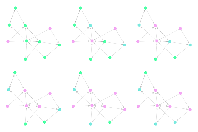
Figure 1: One instance of the bootstrap percolation process with $n=10$ vertices. This percolation process lasts for six rounds until no more additional infections take place. The rounds are ordered from left to right and from top to bottom. The green points are vertices with threshold $2$ that have not received any edge from an infected vertex yet, the darker green points are vertices that have received an edge from exactly one infected vertex, and the violet points are vertices that are infected, either initially or during the process. Note that this graph is directed.

We collect all information about the vertex sequence in the vector $\mathcal{V}\mathrel{\mathop{\ordinarycolon}}=(\kappa,\nu,(\bm{s}(n),\bm{k}(n))_{n\in\mathbb{N}}$ and denote the random graph with $n$ vertices derived from this sequence by $G(n,\mathcal{V})$. The random graph model used here is an adapted version of the model proposed in Bollobás et al. [9], enriched by the threshold values $\bm{k}(n)$ which are crucial parameters for the process we study. While the actual final set of infected vertices $\mathbb{D}(G(n,\mathcal{V}))$ depends on the random graph $G(n,\mathcal{V})$, we will see that under Assumption 2.1 for large $n$, a law or large numbers holds, and we can describe $n^{-1}|\mathbb{D}(G(n,\mathcal{V}))|$ purely in terms of $\kappa$, $\nu$ and $\mathcal{S}$.

2.1 Results

To ignite the bootstrap percolation process, we shall first assume that $\nu(0,\mathcal{S})>0$, which ensures that as $n\rightarrow\infty$ there exists a positive fraction of initially infected vertices, and we then study the final number of infected vertices. Later in Section 2.1.2, we will start with a graph without initial infections, and then study the impact of imposing a small fraction of ex-post infections. This will lead to the idea of the resilience of the random graph.

Assumption 2.2.

We assume that the kernel $\kappa$ is continuous on the space $\mathcal{S}\times\mathcal{S}$, equipped with the product topology.

In light of Assumption 2.2 note that by the Tychonoff theorem, it follows from compactness of $\mathcal{S}$ that $\mathcal{S}\times\mathcal{S}$ is compact with respect to the product topology, and then in particular that $\kappa$ is bounded on $\mathcal{S}\times\mathcal{S}$. We let in the following $M_{\kappa}$ be the bound of $\kappa$. Our main result will show that under Assumption 2.1 and 2.2 the final proportion of infected vertices $n^{-1}|D_{n}|$ can be determined by solving a fixed point equation in some function space.

Remark 2.3.

It would be interesting to allow for discontinuous $\kappa$ or a state space $\mathcal{S}$ that is not compact. This more general model setup has the advantage that $\kappa$ is not necessarily bounded and that one may generate random graphs in which vertices of some type have very large degrees. However, without Assumption 2.2 it appears that even the existence of a first fixed point of the related operators can not be guaranteed, except for some special cases. From a practical perspective, a bounded $\kappa$ is not very restrictive as one may always choose a sufficiently large cutoff. Moreover, to determine the end of the contagion process, it will be necessary to explicitly solve the fixed point equation, which will be challenging numerically if $\kappa$ is unbounded. For the question of resilience that we address in Section 2.1.2, considering unbounded $\kappa$ is however particularly interesting. We leave the analysis in this more general model for future research. Since allowing for bounded but possibly discontinuous $\kappa$ does not significantly enrich the theoretical treatment of the percolation process that we consider, we restrict to a setup that keeps the presentation simpler.

We now introduce the operators which will be important for the analysis of the bootstrap percolation process.

Related operators: Let

$$\mathcal{F}_{b}\mathrel{\mathop{\ordinarycolon}}=\{f\mathrel{\mathop{\ordinarycolon}}\mathcal{S}\rightarrow\mathbb{R}_{+},\text{bounded, Borel}\}$$

the set of bounded positive and Borel measurable functions on $\mathcal{S}$. We equip $\mathcal{F}_{b}$ with the supremum norm $\mathinner{\!\left\lVert\cdot\right\rVert}_{\infty}$ defined by $\mathinner{\!\left\lVert f\right\rVert}_{\infty}\mathrel{\mathop{\ordinarycolon}}=\sup_{s\in\mathcal{S}}\mathinner{\!\left\lvert f(s)\right\rvert}$ which turns $\mathcal{F}_{b}$ into a metric space with metric given by $d(f_{1},f_{2})=\mathinner{\!\left\lVert f_{1}(s)-f_{2}(s)\right\rVert}_{\infty}$. We stress that $\mathcal{F}_{b}$ is actually not a vector space but only a convex cone because it contains only the non-negative functions. Although $\mathcal{F}_{b}$ is not a vector space we will still make use the norm symbol $\mathinner{\!\left\lVert\cdot\right\rVert}_{\infty}$ in many cases which causes no problem since $\mathcal{F}_{b}\subset\{f\mathrel{\mathop{\ordinarycolon}}\mathcal{S}\rightarrow\mathbb{R},\text{bounded, Borel}\}$. We further define

$$\mathcal{F}_{1}\mathrel{\mathop{\ordinarycolon}}=\{f\mathrel{\mathop{\ordinarycolon}}\mathcal{S}\rightarrow[0,1],\text{Borel}\}\subset\mathcal{F}_{b},$$

the subset of those functions that are bounded by $1$.

For convenience, also define the two constant functions $\mathcal{F}_{b}\ni\mathbf{0}\mathrel{\mathop{\ordinarycolon}}\mathcal{S}\rightarrow\{0\}$ and $\mathcal{F}_{b}\ni\mathbf{1}\mathrel{\mathop{\ordinarycolon}}\mathcal{S}\rightarrow\{1\}$. Define the operators $\Lambda_{\kappa}\mathrel{\mathop{\ordinarycolon}}\mathcal{F}_{b}\rightarrow\mathcal{F}_{b},P_{\kappa}^{k}\mathrel{\mathop{\ordinarycolon}}\mathcal{F}_{b}\rightarrow\mathcal{F}_{1}$ and $\Psi_{\kappa}\mathrel{\mathop{\ordinarycolon}}\mathcal{F}_{b}\rightarrow\mathcal{F}_{1}$ by

$$\Lambda_{\kappa}[f](\cdot) \mathrel{\mathop{\ordinarycolon}}=\int_{s\in\mathcal{S}}\kappa(s,\cdot)f(s)\mathrm{d}\mu(s),$$ (2.4)

$$P_{\kappa}^{k}[f](\cdot) \mathrel{\mathop{\ordinarycolon}}=\frac{\left(\Lambda_{\kappa}[f](\cdot)\right)^{k}}{k!}\mathrm{e}^{-\Lambda_{\kappa}[f](\cdot)},$$ (2.5)

$$\Psi_{\kappa}[f](\cdot) \mathrel{\mathop{\ordinarycolon}}=\sum_{k=0}^{\infty}\eta_{k}(\cdot)\left(1-\sum_{k^{\prime}=0}^{k-1}P_{\kappa}^{k^{\prime}}[f](\cdot)\right),$$ (2.6)

where $\eta_{k}(\cdot)$ is the Radon-Nikodym derivative defined in (2.3). We use center-dot notation with bracket $[\cdot]$ for arguments that are function valued $f\in\mathcal{F}_{b}$, and center-dot notation with parenthesis $(\cdot)$ for arguments of type $s\in\mathcal{S}$. For example, for $f,h\in\mathcal{F}_{b}$, $s^{\prime}\in\mathcal{S}$, we evaluate $\Lambda_{\kappa}[f+h](s^{\prime})=\int_{s\in\mathcal{S}}\kappa(s,s^{\prime})[f+h](s)\mathrm{d}\mu(s)$. To keep the notation neat, we will sometimes omit the bracket or parenthesis argument as long as this does not cause any confusion. In the following two lemmas, we state some important properties of the operators defined above. For $f,g\in\mathcal{F}_{b}$, we say that $f\leq g$ if only if $f(s)\leq g(s)$ for all $s\in\mathcal{S}$.

Lemma 2.4 (Monotonicity).

For $f,g\in\mathcal{F}_{b}$ with $f\leq g$ it holds that $\Psi_{\kappa}f\leq\Psi_{\kappa}g$.

Lemma 2.5 (Continuous image of $\Psi_{\kappa}$).

Let $\mathcal{F}_{\cdot}^{c}\mathrel{\mathop{\ordinarycolon}}=\{f\in\mathcal{F}_{\cdot}\mathrel{\mathop{\ordinarycolon}}f\text{ is continuous}\}$, then for all $f\in\mathcal{F}_{b}$, $\Lambda_{\kappa}[f]\in\mathcal{F}_{b}^{c}$, $P_{\kappa}^{k}[f]\in\mathcal{F}_{1}^{c}$ and $\Psi_{\kappa}[f]\in\mathcal{F}_{1}^{c}$. Moreover, if we further assume $\kappa$ to be Lipschitz continuous with constant $L_{\kappa}$, then for all $f\in\mathcal{F}_{b}$, $\Lambda_{\kappa}[f]\in\mathcal{F}_{b}^{Lip}$, $P_{\kappa}^{k}[f]\in\mathcal{F}_{1}^{Lip}$ and $\Psi_{\kappa}[f]\in\mathcal{F}_{1}^{Lip}$, where $\mathcal{F}_{\cdot}^{Lip}\subset\mathcal{F}_{b}$ is defined by $\mathcal{F}_{\cdot}^{Lip}\mathrel{\mathop{\ordinarycolon}}=\{f\in\mathcal{F}_{\cdot}\mathrel{\mathop{\ordinarycolon}}f\text{ is Lipschitz with constant }L_{\kappa}(1+M_{\kappa})M_{\kappa}e^{M_{\kappa}}\}$.

We will see that if a minimal fixed point of the operator $\Psi_{\kappa}$ exists, then it allows us to determine the final proportion of infected vertices. By fixed point, we mean a function $f$ in the convex cone $\mathcal{F}_{b}$ such that $f=\Psi_{\kappa}f$. With a Lipschitz condition on $\kappa$, we can prove the existence of a minimal fixed point of $\Psi_{\kappa}$:

Lemma 2.6 (Existence of the minimal fixed point).

Let $\kappa$ be Lipschitz continuous with constant $L_{\kappa}$ and $\mathcal{F}_{1}^{Lip}$ as defined in Lemma 2.5. Let further $\mathcal{H}\subset\mathcal{F}_{1}^{Lip}$ be the set defined by

$$\mathcal{H}\mathrel{\mathop{\ordinarycolon}}=\{f\in\mathcal{F}_{1}^{Lip}\mathrel{\mathop{\ordinarycolon}}f=\Psi_{\kappa}f\}.$$ (2.7)

Then $\mathcal{H}$ is not empty and includes all the fixed points. Each $h\in\mathcal{H}$ is continuous and there exists a function $\eta_{0}\leq\hat{f}\in\mathcal{H}$ such that $\hat{f}\leq h$ for every $h\in\mathcal{H}$. We call $\hat{f}$ the minimal fixed point. Clearly, it then also holds that $\int_{\mathcal{S}}\hat{f}\mathrm{d}\mu=\min_{f\in\mathcal{H}}\big{\{}\int_{\mathcal{S}}f\mathrm{d}\mu\big{\}}$.

The proof of Lemma 2.5 relies on an argument that requires us to find a subset $\mathcal{H}_{1}\subset\mathcal{F}_{b}$ of measurable functions that contains all fixed points of $\Psi_{\kappa}$ (if any) and which is such that for any subset $\mathcal{H}_{2}\subset\mathcal{H}_{1}$ the pointwise supremum (respectively infimum) of the functions in $\mathcal{H}_{2}$ is a function in $\mathcal{H}_{1}$. Because the supremum of measurable functions is not measurable in general, we need to choose a continuity property that is stable under taking the supremum. Without the assumption that $\kappa$ is Lipschitz continuous, it is therefore in general not possible to show the existence of a minimal fixed point, except for some special cases where $\kappa$ is either of a particular structural form, or the thresholds of the vertices are all either $0$ or $1$.

Next, we shall specify the "Fréchet derivative" on a convex cone. Recall that $\mathcal{F}_{b}$ is a convex cone such that $af_{1}+bf_{2}\in\mathcal{F}_{b}$ for $f_{1},f_{2}\in\mathcal{F}_{b}$ and any non-negative scalar $a,b\geq 0$. Though the Fréchet derivative is usually defined on a vector space, it can be defined in the same spirit on $\mathcal{F}_{b}$. Let $L^{+}(\mathcal{F}_{b})\subset C(\mathcal{F}_{b},\mathcal{F}_{b})$ be a subset of continuous functions which are non-negative and closed under linear combinations with non-negative scalar. For an operator $\Phi\mathrel{\mathop{\ordinarycolon}}\mathcal{F}_{b}\rightarrow\mathcal{F}_{b}$, we call $D\Phi\mathrel{\mathop{\ordinarycolon}}\mathcal{F}_{b}\rightarrow L^{+}(\mathcal{F}_{b})$ the Fréchet derivative of $\Phi$ in $L^{+}(\mathcal{F}_{b})$ if for all $f,h\in\mathcal{F}_{b}$ it holds

$$\lim_{\mathinner{\!\left\lVert h\right\rVert}_{\infty}\rightarrow 0}\frac{\mathinner{\!\left\lVert\Phi(f+h)-\Phi(f)-D\Phi f[h]\right\rVert}_{\infty}}{\mathinner{\!\left\lVert h\right\rVert}_{\infty}}=0.$$ (2.8)

Lemma 2.7 (Fréchet derivative).

The operator $\Psi_{\kappa}\mathrel{\mathop{\ordinarycolon}}\mathcal{F}_{b}\rightarrow\mathcal{F}_{b}$ is Fréchet differentiable at every point $f\in\mathcal{F}_{b}$ and the derivative $D\Psi_{\kappa}\mathrel{\mathop{\ordinarycolon}}\mathcal{F}_{b}\rightarrow L^{+}(\mathcal{F}_{b})$, is given by

$$D\Psi_{\kappa}f[\cdot](\cdot)=\Lambda_{\kappa}[\cdot](\cdot)V[f](\cdot)$$ (2.9)

where $V[f](\cdot)\mathrel{\mathop{\ordinarycolon}}=\sum_{k=1}^{\infty}\eta_{k}(\cdot)P_{\kappa}^{k-1}f(\cdot)$.

2.1.1 Final Set of Infected Vertices

We are now ready to state our first main result about the final number of infected vertices.

Theorem 2.8 (Final fraction of infected vertices).

Let $\mathcal{V}$ be a vertex sequence with resulting random graph $G(n,\mathcal{V})$ and assume that a minimal fixed point $\hat{f}$ of $\Psi_{\kappa}$ exists. Then the following holds:

1. For every $\varepsilon>0$ it holds that

   $$\lim_{n\rightarrow\infty}\mathds{P}\left(n^{-1}|\mathbb{D}(G(n,\mathcal{V}))|\geq\int_{\mathcal{S}}\hat{f}\mathrm{d}\mu-\varepsilon\right)=1.$$ (2.10)

2. If, in addition, there exists some non-negative and continuous function $h\in\mathcal{F}_{b}$ and small $\epsilon>0$ such that

   $$D\Psi_{\kappa}\hat{f}[h]-h<-\epsilon\mathbf{1},$$ (2.11)

   then

   $$n^{-1}|\mathbb{D}(G(n,\mathcal{V}))|\xrightarrow[n\rightarrow\infty]{p}\int_{\mathcal{S}}\hat{f}\mathrm{d}\mu.$$ (2.12)

In particular for the case of $\kappa$ Lipschitz, we know by Lemma 2.6 that a minimal fixed point exists. Except for some pathological cases, then also the derivative condition holds and Theorem 2.8 allows us to determine the final fraction of infected vertices at the end of the bootstrap percolation process.

To gain some intuition for this result, let us give some heuristic interpretation. Note that a vertex of type $s^{\prime}\in\mathcal{S}$ has a degree that is approximately Poisson distributed with parameter

$$\Lambda_{\kappa}[\mathbf{1}](s^{\prime})=\int_{s\in\mathcal{S}}\kappa(s,s^{\prime})d\mu(s).$$

At the end of the process, some fraction $\hat{f}(s)$ of all vertices of type $s\in\mathcal{S}$ will be infected. If we would now add a new vertex of type $s^{\prime}$ with a threshold value equal to $k$ to the graph and connect this vertex to the existing vertices with probability described by the kernel and all edges independent, then that vertex has a degree to the set of infected vertices that is Poisson distributed with parameter given by

$$\Lambda_{\kappa}[\hat{f}](s^{\prime})=\int_{s\in\mathcal{S}}\kappa(s,s^{\prime})\hat{f}(s)d\mu(s),$$

and the probability of it being infected is given by

$$1-\sum_{k^{\prime}=0}^{k-1}P_{\kappa}^{k^{\prime}}[\hat{f}](s^{\prime}),$$ (2.13)

which is the probability that a Poisson distributed random variable with parameter $\Lambda_{\kappa}[\hat{f}](s^{\prime})$ is larger or equal to $k$. Surprisingly, it turns out that despite the complicated dependency of the degree of a vertex in the graph and its state of infection, an existing uniformly selected vertex of the graph, conditioned on its threshold being $k$ and its type being $s^{\prime}$, has a probability of being infected given by (2.13). Summing up over the proportion of all vertices with type $s^{\prime}$ but possibly different threshold leads to the fixed point condition. The derivative condition (2.11) is required to exclude an unstable equilibrium in which the additional default of a few vertices could restart the process, leading to many additional infections. The condition ensures that when almost $\hat{f}(s)$ of type $s$ vertices are infected for every $s\in\mathcal{S}$, the exploration of another infected vertex leads on average to less than one additional infected vertex.

2.1.2 Resilience

In the previous section, we studied the final set of infected vertices for a random graph with a positive fraction of initially infected vertices, i.e. $\nu_{0}(\mathcal{S})>0$. We now look at an initially uninfected graph and want to make statements about the resilience of the graph to ex-post infections. In order to keep our notation consistent, we adapt the previous notation of the random graph and related operators for the ex-post infected graph and denote the quantities related to the uninfected graph with a tilde instead, i.e. for the uninfected graph we have $\widetilde{\nu}_{0}(\mathcal{S})=0$. Assume that ex-post we infect some vertices by setting their threshold value to $0$ while we keep all other thresholds unchanged. A question that arises naturally is then whether there exists a lower bound $\Delta$ for the fraction of infected vertices such that any ex-post infection leads to at least $\Delta n$ infected vertices at the end of the process. If that is the case, the graph is considered non-resilient. On the contrary, we call it resilient if a reduction of the fraction of initially infected vertices to $0$ ensures that also the final fraction of infected vertices goes to $0$.

To formalize the setup, let $\widetilde{\mathcal{V}}\mathrel{\mathop{\ordinarycolon}}=(\kappa,\widetilde{\nu},(\bm{s}(n),\widetilde{\bm{k}}(n))_{n\in\mathbb{N}}$ be a vertex sequence that fulfils Assumption 2.1 and that is such that $\widetilde{\nu}(0,\mathcal{S})=0$. For each $n\in\mathbb{N}$, we now define a new threshold sequence $\bm{k}(n)=(k_{1}(n),\dots,k_{n}(n))$ which is such that for each $n\in\mathbb{N},1\leq i\leq n$ either $k_{i}(n)=\widetilde{k}_{i}(n)$ or $k_{i}(n)=0$. For $k\in\mathbb{N}$ and Borel set $A\subset\mathcal{S}$, define

$$\nu^{(n)}(k,A)\mathrel{\mathop{\ordinarycolon}}=n^{-1}\sum_{i\in[n]}I_{\{k\}}(k_{i})I_{A}(s_{i}).$$

We further assume that for the new sequence there exists again a measure $\nu$ on $\mathbb{N}_{0}\times\mathcal{S}$ such that for each fixed $k$, the measure $\nu(k,\cdot)$ is a Borel measure on $\mathcal{S}$ and that for every $k\in\mathbb{N}_{0}$ and Borel set $A$ it holds that:

$$\nu^{(n)}(k,A)\stackrel{{\scriptstyle[}}{{n}}\rightarrow\infty]{}{\longrightarrow}\nu(k,A).$$ (2.14)

Moreover, we assume that $\nu(0,\mathcal{S})>0$, so as a result of the threshold changes a fraction of vertices is infected as $n\rightarrow\infty$, and these infected vertices start the percolation process. Let as before $\mathcal{V}\mathrel{\mathop{\ordinarycolon}}=(\kappa,\nu,(\bm{s}(n),\bm{k}(n))_{n\in\mathbb{N}}$.

By construction of $\widetilde{\mathcal{V}}$ and $\mathcal{V}$ we have the following relations for all Borel sets $A\subset\mathcal{S}$:

$$\widetilde{\nu}(k,A)-\nu(k,A)\geq 0\text{ for }k\geq 1 \widetilde{\nu}(0,A)=\sum_{k=1}^{\infty}\widetilde{\nu}(k,A)-\nu(k,A).$$ (2.15)

In the same fashion of (2.3), for subset $A\subset\mathcal{S}$, we denote the marginal distribution and the Radon-Nikodym derivative by

$$\widetilde{\mu}(A)\equiv\mu(\cdot)\mathrel{\mathop{\ordinarycolon}}=\sum_{k=0}^{\infty}\nu(k,A), \widetilde{\nu}(k,A)=\int_{A}\widetilde{\eta}_{k}(s)\mathrm{d}\widetilde{\mu}(s), \nu(k,A)=\int_{A}\eta_{k}(s)\mathrm{d}\mu(s).$$ (2.16)

We now define resilience and non-resilience as follows:

Definition 2.9.

Let $\widetilde{\mathcal{V}}$ be the initial uninfected vertex sequence and $\mathcal{V}$ the vertex sequence with ex-post infections. As before denote by $G(n,\widetilde{\mathcal{V}})$ and $G(n,\mathcal{V})$ the corresponding random graphs and note that they both have exactly the same skeleton distribution and differ only in terms of their threshold values.

We call the random graph $G(n,\widetilde{\mathcal{V}})$

1. non-resilient, if there exists an $\Delta>0$ only depending on $\widetilde{\nu}$ such that $|\mathbb{D}(G(n,\mathcal{V}))|/n\geq\Delta$, for $n$ large, independent of the precise specification of $\nu$.

2. resilient, if for all $\alpha>0$, there exists $\delta>0$ such that $|\mathbb{D}(G(n,\mathcal{V}))|/n<\alpha$ for $0<\nu(0,\mathcal{S})<\delta$.

In other words, for a non-resilient graph, no matter how small the initial infection is, the final fraction of infected vertices will always exceed a certain level, while, for a resilient graph, the final fraction of infected vertices is small as long as the initial infection is small. In the following, we provide a condition that allows us to determine whether a random graph is resilient or non-resilient. Introduce the two operators $\widetilde{\Psi}\mathrel{\mathop{\ordinarycolon}}\mathcal{F}_{b}\rightarrow\mathcal{F}_{b}$ and $\Psi\mathrel{\mathop{\ordinarycolon}}\mathcal{F}_{b}\rightarrow\mathcal{F}_{b}$ corresponding to the uninfected $G(n,\widetilde{\mathcal{V}})$ and the infected graph $G(n,\mathcal{V})$:

$$\widetilde{\Psi}[f](\cdot)\mathrel{\mathop{\ordinarycolon}}=\sum_{k=0}^{\infty}\widetilde{\eta}_{k}(\cdot)\left(1-\sum_{k^{\prime}=0}^{k-1}P_{\kappa}^{k^{\prime}}[f](\cdot)\right), \Psi[f](\cdot)\mathrel{\mathop{\ordinarycolon}}=\sum_{k=1}^{\infty}\eta_{k}(\cdot)\left(1-\sum_{k^{\prime}=0}^{k-1}P_{\kappa}^{k^{\prime}}[f](\cdot)\right),$$ (2.17)

where $P_{\kappa}^{k}$ is as defined in equation (2.4). Note that the summation of $\widetilde{\Psi}$ starts from $k=1$ as $\widetilde{\nu}(0,\mathcal{S})=0$. Also, for $\widetilde{\Psi}f$ we can calculate the Fréchet derivative $D\widetilde{\Psi}f$ as in equation (2.9). The following theorem provides the resilience condition.

Theorem 2.10 (Resilience).

If there exists a continuous and non-negative function $h\in\mathcal{F}_{b}$ such that

1. $D\widetilde{\Psi}\mathbf{0}[h]>h$. Then, the graph is non-resilient.

2. $D\widetilde{\Psi}\mathbf{0}[h]<h$. Then, the graph is resilient.

Moreover, the graph cannot be both non-resilient and resilient, i.e. there do not exit functions $h,g\in\mathcal{F}_{b}$ such that $D\widetilde{\Psi}\mathbf{0}[h]>h$ and $D\widetilde{\Psi}\mathbf{0}[g]<g$ hold at the same time. Note that $D\widetilde{\Psi}\mathbf{0}[h]$ is the Fréchet derivative of the operator $\widetilde{\Psi}$ at the point $\mathbf{0}$, applied to $h$.

Remark 2.11.

It is worth noting that our notion of resilience is in some cases related to the existence of a giant component. Bollobás et al. [9] proved in their Theorem 3.1 that a giant component exists if the $\mathcal{L}^{2}$ norm of the operator $\Lambda_{\kappa}$ is larger than $1$. In our model, if all the vertices have a threshold equal to one, then our condition 1. implies that the $\mathcal{L}^{2}$ norm of $\Lambda_{\kappa}$ is larger than $1$ and the network must have a giant component.

2.2 Proof Strategy

2.2.1 Final Fraction of Infected Vertices

We provide a sketch of the proof ideas which are carried out in detail in Appendix A and B.

We first derive a sequence of partitions of the space $\mathcal{S}$. Based on this sequence of partitions we can then define coupling kernels $\kappa_{L}^{+}$ and $\kappa_{L}^{-}$ for $L\in\mathbb{N}$, which are step functions that dominate the original kernel from above and below, and which, in addition to some other properties, are such that the first fixed points of $\Psi_{\kappa_{L}^{-}}$ and $\Psi_{\kappa_{L}^{+}}$ converge to the first fixed point of $\Psi_{\kappa}$. Collapsing the types in each subset into a single type, these coupling kernels then lead to two sequences of random graphs, one which has more edges than the original graph, and another one with fewer edges. This leads to upper and lower bounds of $|\mathbb{D}(G(n,\mathcal{V}))|$ in terms of the final fraction of infected vertices in this finite-type graph. We can then show that the final number of infected vertices in the finite-type random graphs can be obtained as a solution to a finite-dimensional fixed point equation. However, in this approximation, the dimension of the related fixed point equation is actually finite and increasing in $L$ and the connection to the operator equation $\Psi[\hat{f}]=\hat{f}$ is not straightforward at first. However, we can embed the finite-dimensional system into the original system, which then lets us show that not only the operators $\Psi_{\kappa_{L}^{\pm}}$ are converging but also the fraction of infected vertices. In this section, we describe the required auxiliary results and the embedding in more detail. In Section 2.2.2 we explain the proof strategy for our resilience result. All proofs are then carried out in detail in Appendix A and Appendix B.

The following lemma provides the basis for the construction of our approximating graph sequence:

Lemma 2.12.

There exists a sequence, indexed by $L\in\mathbb{N}$, of measurable partitions $\{\mathcal{S}_{L}^{l}\}_{l\in[N(L)]}$ of $\mathcal{S}$, where $N(L)$ is the finite number of subsets, such that

1. $\{\mathcal{S}_{L^{\prime}}^{l}\}_{l\in[L^{\prime}]}$ for each $L^{\prime}>L$ is a refinement of $\{\mathcal{S}_{L}^{l}\}_{l\in[N(L)]}$, i.e. each $\mathcal{S}_{L}^{l}$ is a union $\cup_{j\in J}\mathcal{S}_{L^{\prime}}^{j}$ for some set $J\subset N(L^{\prime})$.

2. As $L\rightarrow\infty$, $\mu(S_{L}^{l})\rightarrow 0$ $\forall l\in[N(L)]$.

Based on the partition in the previous lemma we can now define kernels that are step functions and are the basis for defining our coupling graphs.

Definition 2.13 (Coupling graphs).

For $G(n,\mathcal{V})$, we construct two sequences of coupling graphs indexed by $N\in\mathbb{N}$ as follows. Partition the type space $\mathcal{S}$ into $N(L)$ subsets according to Lemma 2.12. Define two stepwise kernel functions by

$$\kappa_{L}^{+}(s,s^{\prime}) \mathrel{\mathop{\ordinarycolon}}=\sum_{l,l^{\prime}\in[N(L)]}I_{\mathcal{S}^{l}}(s)I_{\mathcal{S}^{l^{\prime}}}(s^{\prime})\sup_{x\in\mathcal{S}^{l},y\in\mathcal{S}^{l^{\prime}}}\kappa(x,y),$$ (2.18)

$$\kappa_{L}^{-}(s,s^{\prime}) \mathrel{\mathop{\ordinarycolon}}=\sum_{l,l^{\prime}\in[N(L)]}I_{\mathcal{S}^{l}}(s)I_{\mathcal{S}^{l^{\prime}}}(s^{\prime})\inf_{x\in\mathcal{S}^{l},y\in\mathcal{S}^{l^{\prime}}}\kappa(x,y),$$ (2.19)

where $I_{\mathcal{S}_{L}^{l}}(s)$ is the indicator function taking value $1$ if $s\in\mathcal{S}_{L}^{l}$, otherwise $0$. With these stepwise kernels $\kappa_{L}^{-}$ and $\kappa_{L}^{+}$ which are such that $\kappa_{L}^{-}\leq\kappa\leq\kappa_{L}^{+}$, we can now specify two vertex sequences $\mathcal{V}_{L}^{-}\mathrel{\mathop{\ordinarycolon}}=(\kappa_{L}^{-},\nu,(\bm{s}(n),\bm{k}(n))$ and $\mathcal{V}_{L}^{+}\mathrel{\mathop{\ordinarycolon}}=(\kappa_{L}^{+},\nu,(\bm{s}(n),\bm{k}(n))$, that define random graphs $G(n,\mathcal{V}_{L}^{-})$ and $G(n,\mathcal{V}_{L}^{+})$. These graphs now couple the original graph $G(n,\mathcal{V})$ in the following sense: For any pair of vertices $i,j\in[n]$ in a graph $G$, let $E_{i,j}(G)\mathrel{\mathop{\ordinarycolon}}=I_{\{i\text{ connects to }j\text{ in graph }G\}}$ be the indicator of an edge from $i$ to $j$. By construction we can now ensure that $E_{i,j}(G(n,\mathcal{V}_{L}^{-}))\leq E_{i,j}(G(n,\mathcal{V}))\leq E_{i,j}(G(n,\mathcal{V}_{L}^{+}))$. One way to generate such coupling systems, for example, is by uniform random variables to generate edges as follows. For each pair of vertices $i,j\in[n]$, generate $U\sim\text{Uniform([0,1])}$, and set the edge by $E_{i,j}(G(n,\mathcal{V}_{L}^{-})=I_{\{U\leq\kappa_{L}^{-}(s_{i},s_{j})\}}$, $E_{\kappa_{L}}(i,j)=I_{\{U\leq\kappa_{L}(s_{i},s_{j})\}}$, and $E_{i,j}(G(n,\mathcal{V}_{L}^{+})=I_{\{U\leq\kappa_{L}^{+}(s_{i},s_{j})\}}$. As a result, we have that $E_{i,j}(G(n,\mathcal{V}_{L}^{-}))\leq E_{i,j}(G(n,\mathcal{V}))\leq E_{i,j}(G(n,\mathcal{V}_{L}^{+}))$ as desired, and for the total number of infected vertices after the percolation it follows that

$$|\mathbb{D}(G(n,\mathcal{V}_{L}^{-}))|\leq|\mathbb{D}(G(n,\mathcal{V}))|\leq|\mathbb{D}(G(n,\mathcal{V}_{L}^{+}))|.$$ (2.20)

In this sense, we call $G(n,\mathcal{V}_{L}^{-})$ a lower coupling graph of $G(n,\mathcal{V})$ and $G(n,\mathcal{V}_{L}^{+})$ an upper coupling graph of the original $G(n,\mathcal{V})$.

By the construction of the coupling graphs, we hope that we can determine $|\mathbb{D}(G(n,\mathcal{V}_{L}^{\pm}))|$, and that $|\mathbb{D}(G(n,\mathcal{V}_{L}^{\pm}))|$ will converge to $|\mathbb{D}(G(n,\mathcal{V}))|$ as the partitions for $\mathcal{S}$ get finer as $L\rightarrow\infty$. Because the kernels $\kappa_{L}^{\pm}$ are step functions it holds that $\kappa_{L}^{\pm}(s,s^{\prime})=\kappa_{L}^{\pm}(r,r^{\prime})$ for any $s,r\in\mathcal{S}_{L}^{l}$ and $s^{\prime},r^{\prime}\in\mathcal{S}_{L}^{l^{\prime}}$, i.e. the connection probability $\kappa_{L}^{\pm}(s,s^{\prime})$ equals to $\kappa_{L}^{\pm}(r,r^{\prime})$ for any pair of types in the same type intervals. Hence, for all the vertices we only need to know the index $l$ of the set $\mathcal{S}_{L}^{l}$ that they belong to in order to determine their connection probabilities, and therefore we can just assign the integer $l\in[N(L)]$ as a type and define a discrete kernel $\kappa^{\pm d}_{L}\mathrel{\mathop{\ordinarycolon}}[N(L)]^{2}\rightarrow\mathbb{R}_{+}$ accordingly. This leads to a random graph with the same skeleton distribution as the one defined by $\kappa_{L}^{\pm}$. By this grouping of the vertex types, we can turn the coupling graphs into graphs of finitely many vertex types with a discrete kernel function. Denote this random graph by $G(n,\mathcal{V}_{L}^{d,\pm})$. It follows obviously that

$$|\mathbb{D}(G(n,\mathcal{V}_{L}^{\pm}))|=|\mathbb{D}(G(n,\mathcal{V}_{L}^{d,\pm}))|.$$ (2.21)

We then first investigate the final fraction of infected vertices in the graph $G(n,\mathcal{V}_{L}^{d,\pm})$.

Definition 2.14 (Graph with finite vertex type).

For fixed $N(L)$ we consider a random graph with vertices having types in the set $[N(L)]$ and thresholds $k\in\mathbb{N}_{0}$. The proportion of vertices with certain threshold and type is now described by the numbers $(\mathbf{\nu}^{l,(n)}_{k})_{l\in[N(L)],\ k\in\mathbb{N}_{0}}$, where

$$\mathbf{\nu}^{l,(n)}_{k}(A)=n^{-1}\sum_{i\in[n]}I_{\{k\}}(k_{i})I_{\{l\}}(s_{i})$$ (2.22)

is their proportion. As before, we assume that there exists $\{\mathbf{\nu}^{l}_{k}\}_{l\in[N(L)],\ k\in\mathbb{N}_{0}}$ such that

$$\mathbf{\nu}^{l,(n)}_{k}\stackrel{{\scriptstyle[}}{{n}}\rightarrow\infty]{}{\longrightarrow}\mathbf{\nu}^{l}_{k},$$ (2.23)

i.e. the proportion of vertices with a certain type and threshold converges. For the connection probability, we define a discrete kernel $\kappa^{d}_{L}\mathrel{\mathop{\ordinarycolon}}[N(L)]^{2}\rightarrow\mathbb{R}$. Note that we use a superscript $d$ to distinguish the kernel defined on $[N(L)]^{2}$ from the one defined on $\mathcal{S}^{2}$. Then, for $i,j\in[n]$, the connection probability is given by $\min\{1,\kappa^{d}_{L}(l_{i},l_{j})/n\}$. Again we define the vertex sequence $\mathcal{V}_{L}^{d}\mathrel{\mathop{\ordinarycolon}}=(\kappa^{d}_{L},\nu,(\bm{s}(n),\bm{k}(n))$ for this graph and denote by $G(n,\mathcal{V}_{L}^{d})$ the resulting random graph.

For this finite-type vertex sequence, it turns out that the percolation process can be fully described by the solution of a system of ordinary differential equations of dimension $N(L)$. The final fraction of infected vertices $n^{-1}|\mathbb{D}(G(n,\mathcal{V}_{L}^{d}))|$ is then determined from the first joint zero of this system. While we postpone the formal derivations and discussions to Appendix A, we state and explain the solution functions here. For $l\in[N(L)]$ and $k\in\mathbb{N}_{0}$, we define the functions $\nu_{k}^{l}\mathrel{\mathop{\ordinarycolon}}[0,1]^{N(L)}\rightarrow\mathbb{R}$ by

$$\nu_{0}^{l}(\mathbf{z}) =-z^{l}+\nu_{0}^{l}(\mathbf{0})+\sum_{k^{\prime}=1}^{\infty}\nu_{k^{\prime}}^{l}(\mathbf{0})\left(1-\sum_{k^{\prime\prime}=0}^{k^{\prime}-1}p(k^{\prime\prime},\lambda^{l}(\mathbf{z})\right)$$ (2.24)

$$\nu_{k}^{l}(\mathbf{z}) =\sum_{k^{\prime}=k}^{\infty}\nu_{k^{\prime}}^{l}(\mathbf{0})p(k^{\prime}-k,\lambda^{l}(\mathbf{z})),\ \forall k\geq 1,$$ (2.25)

where $\nu_{k}^{l}(\mathbf{0})$ is the initial proportion of vertices with type $l$ and threshold $k$, $p(k,\lambda)\mathrel{\mathop{\ordinarycolon}}=\tfrac{\lambda^{k}}{k!}\mathrm{e}^{-\lambda}$ is a Poisson probability function, $\mathbf{z}\mathrel{\mathop{\ordinarycolon}}=\{z^{l}\}_{l\in[N(L)]}\in[0,1]^{N(L)}$ is an $N(L)$-dimensional vector, and $\lambda^{l}(\mathbf{z})\mathrel{\mathop{\ordinarycolon}}=\sum_{l^{\prime}\in[N(L)]}\kappa(l^{\prime},l)z^{l^{\prime}}$. The quantities $\mathbf{z}$, $\lambda$, and $p(k,\lambda)$ are the discrete counterparts of the operators $f$, $\Lambda$ and $P$ defined in (2.4). In a sequential formulation of the process that we introduce in Appendix A, the function $\nu_{k}^{l}$ tracks the number of vertices of type $l$ that need another $k$ infected neighbors to become infected themselves. The argument vector contains for each type $l\in[N(L)]$, the fraction of vertices of this type that are infected and whose impact on the system has already been explored.

In Appendix A, we show that if we find

$$\widehat{\mathbf{z}}\mathrel{\mathop{\ordinarycolon}}=\operatorname*{argmin}_{\mathbf{z}}\left\{\sum_{l\in[N(L)]}z^{l}\mathrel{\mathop{\ordinarycolon}}\left\{\nu_{0}^{l}(\mathbf{z})\right\}_{l\in[N(L)]}=\mathbf{0}\right\},$$ (2.26)

and a condition on the partial derivative of the multivariate function $\{\nu_{0}^{l}(\mathbf{z})\}_{l\in[N(L)]}$ in $\widehat{\mathbf{z}}$ holds, then $|\mathbb{D}(G(n,\mathcal{V}_{L}))|/n$, the total proportion of infected vertices in $G(n,\mathcal{V}^{d}_{L})$, will asymptotically converge to $\sum_{l\in[N(L)]}\widehat{z}^{l}$.

Now, having the formulas introduced above, we are able to formalize how we can embed the finite-dimensional description of the process for the random graph $G(n,\mathcal{V}_{L}^{d})$ into the operator $\Psi_{\kappa_{L}}$ which is based on a step function kernel $\kappa_{L}$.

Definition 2.15 (Embedded finite-dimensional functions).

Divide the space $\mathcal{S}$ into $L$ subsets $(\mathcal{S}_{L}^{l})_{l\in[N(L)]}$ the same way as in Definition 2.13, then define the step functions $\kappa_{L}(s,s^{\prime})\mathrel{\mathop{\ordinarycolon}}\mathcal{S}\times\mathcal{S}\rightarrow\mathbb{R}$ and for $\mathbf{z}\in[0,1]^{N(L)}$ the function $f_{L}(s)\mathrel{\mathop{\ordinarycolon}}\mathcal{S}\rightarrow[0,1]$ as

$$\kappa_{L}(s,s^{\prime})\mathrel{\mathop{\ordinarycolon}}=\sum_{l,l^{\prime}\in[N(L)]}I_{\mathcal{S}^{l}}(s)I_{\mathcal{S}^{l^{\prime}}}(s^{\prime})\kappa^{d}_{L}(l,l^{\prime}), f_{L}(s)\mathrel{\mathop{\ordinarycolon}}=\sum_{l\in[N(L)]}\frac{1}{\mu(\mathcal{S}_{L}^{l})}z_{L}^{l}I_{\mathcal{S}_{L}^{l}}(s),$$ (2.27)

The following equality holds:

$$\nu_{0}^{l}(\mathbf{z}_{L}) =-z_{L}^{l}+\sum_{k^{\prime}=0}^{\infty}\nu_{k^{\prime}}^{l}(\mathbf{0})\left(1-\sum_{k^{\prime\prime}=0}^{k^{\prime}-1}p(k^{\prime\prime},\lambda^{j}(\mathbf{z}_{L}))\right)$$ (2.28)

$$=-\int_{\mathcal{S}_{L}^{l}}f_{L}(s)\mathrm{d}\mu(s)+\int_{\mathcal{S}_{L}^{l}}\Psi_{\kappa_{L}}[f_{L}](s)\mathrm{d}\mu(s),$$ (2.29)

where $\nu_{0}^{l}(\mathbf{z}_{L})$ and $\nu_{k}^{l}(\mathbf{0})$ are defined in equation (2.24). Because all fixed points of $\Psi_{\kappa_{L}}$ are step functions, this will then allow us to conclude that the first zero $\widehat{z}_{L}^{l}$ of $\{\nu_{0}^{l}(\mathbf{z})\}_{l\in[N(L)]}$ and the first fixed point $\hat{f}_{L}$ of $\Psi_{\kappa_{L}}$ are related by

$$\hat{f}_{L}(s)\mathrel{\mathop{\ordinarycolon}}=\sum_{l\in[N(L)]}\frac{1}{\mu(\mathcal{S}_{L}^{l})}\widehat{z}_{L}^{l}I_{\mathcal{S}_{L}^{l}}(s)$$ (2.30)

and therefore

$$\sum_{l\in[N(L)]}\widehat{z}_{L}^{l} =\int_{\mathcal{S}}\hat{f}_{L}(s)\mathrm{d}\mu(s).$$ (2.31)

Moreover, for $0<w_{l}<1,\ \sum_{l\in[N(L)]}w_{j}=1$ and $h_{L}\in\mathcal{F}_{b}$ defined by

$$h_{L}(s)\mathrel{\mathop{\ordinarycolon}}=\sum_{l\in[N(L)]}\tfrac{1}{\mu(\mathcal{S}_{L}^{l})}w^{l}I_{\mathcal{S}_{L}^{l}}(s),$$ (2.32)

it holds that

$$\sum_{l^{\prime}\in[N(L)]}w^{l^{\prime}}\frac{\partial\nu_{0}^{l}(\mathbf{z}_{L})}{\partial z^{l^{\prime}}} =-w^{l}+\left(\sum_{l^{\prime}\in[N(L)]}\kappa_{L}^{d}(l^{\prime},l)w^{l^{\prime}}\right)\nu_{1}^{l}(\mathbf{z}_{L})$$ (2.33)

$$=-\int_{\mathcal{S}_{L}^{l}}h_{L}(s)\mathrm{d}\mu(s)+\int_{\mathcal{S}_{L}^{l}}D\Psi_{\kappa_{L}}f_{L}[h_{L}](s)\mathrm{d}\mu(s).$$ (2.34)

On the left hand side we have the directional derivative of the multivariate function $\{\nu_{0}^{l}(\mathbf{z})\}_{l\in[N(L)]}$ while on the right hand side we have an expression that involves the Fréchet derivative in the direction $h_{L}$. The identity will allow us to derive stopping criteria for the percolation process in $G(n,\mathcal{V}_{L}^{d})$ from the Fréchet derivative of $\Psi_{\kappa}$. Because of the above equalities, we say that $G(n,\mathcal{V}_{L}^{d})$ can be embedded into $G(n,\mathcal{V}_{L})$. Because $|\mathbb{D}(G(n,\mathcal{V}_{L}^{\pm}))|=|\mathbb{D}(G(n,\mathcal{V}_{L}^{d,\pm}))|$, these equalities allow us to show that the set of infected vertices is related to the fixed point of $\Psi_{\kappa_{L}}$.

In the following simple lemma, we state some convergence properties of the operators $\Psi_{\kappa_{L}^{\pm}}$ to $\Psi_{\kappa}$ on $\mathcal{F}_{b}$ as $L\rightarrow\infty$, which will then be used in the next proposition to prove the convergence of fixed points of $\Psi_{\kappa_{L}^{\pm}}$ to the fixed point $\Psi_{\kappa}$.

Lemma 2.16 (Uniform convergence of operators).

For $f,h\in\mathcal{F}_{b}$ and a monotone sequence $\{f_{L}\}\in\mathcal{F}_{b}$ such that $f_{L}\rightarrow f$ point-wise as $L\rightarrow\infty$, it holds

$$\Psi_{\kappa_{L}^{\pm}}f_{L}\rightarrow\Psi_{\kappa}f, D\Psi_{\kappa_{L}^{\pm}}f_{L}[h]\rightarrow D\Psi_{\kappa}f[h],$$ (2.35)

uniformly in $\mathcal{S}$.

Proposition 2.17 (Uniform convergence of fixed points).

Assume that a minimal fixed $\hat{f}$ of $\Psi_{\kappa}$ exists and that there exists a non-negative continuous function $h\in\mathcal{F}_{b}$ and small $\epsilon>0$ such that $D\Psi_{\kappa}\hat{f}[h]-h<-\epsilon\mathbf{1}$. Then each of the $\Psi_{\kappa^{\pm}_{L}}$ has a minimal fixed point, denoted by $\hat{f}_{L}^{\pm}$. The fixed point $\hat{f}_{L}^{\pm}$ is a step function that is constant on the sets $\{\mathcal{S}^{l}_{L}\}_{l\in N(L)}$. Moreover, as $L\rightarrow\infty$, the following convergences holds:

$$\hat{f}_{L}^{\pm}\rightarrow\hat{f}\text{ uniformly}, D\Psi_{\kappa^{\pm}_{L}}\hat{f}_{L}^{\pm}\rightarrow D\Psi_{\kappa}\hat{f}\text{ uniformly}, \int_{\mathcal{S}}\hat{f}_{L}^{\pm}\mathrm{d}\mu\rightarrow\int_{\mathcal{S}}\hat{f}\mathrm{d}\mu.$$ (2.36)

Remark 2.18.

Proposition 2.17 shows that the minimal fixed points of the coupling operators $\Psi_{\kappa_{L}^{\pm}}$ converge to the minimal fixed points of $\Psi_{\kappa}$. While Lemma 2.16 follows relatively straightforward from assumptions on $\kappa$ and the definition of $\Psi$, showing fixed point convergence is more involved. In our case an additional complication arises due to the increasing dimension of the step functions which depends on $L$.

Now combining (2.20) and (2.21) one obtains that

$$|\mathbb{D}(G(n,\mathcal{V}_{L}^{d,-}))|\leq|\mathbb{D}(G(n,\mathcal{V}))|\leq|\mathbb{D}(G(n,\mathcal{V}_{L}^{d,+}))|.$$ (2.37)

Then $|\mathbb{D}(G(n,\mathcal{V}_{L}^{d,-}))|$ and $|\mathbb{D}(G(n,\mathcal{V}_{L}^{d,+}))|$ can be determined based on the first zero of the functions (2.24). The embedding described in (2.31) and (2.33) allows us to connect the finite dimensional discrete description to the operators $\Psi_{\kappa_{L}^{\pm}}$. Together with Proposition 2.17 we can then show that above inequalities shrink together and determine $|\mathbb{D}(G(n,\mathcal{V}))|$.

2.2.2 Resilience

For the proof of non-resilience, one first notes that the existence of a function $h\in\mathcal{F}_{b}$ such that $D\widetilde{\Psi}\mathbf{0}[h]>h$ implies that by continuity of the derivative, there exists $\alpha>0$ such that $\widetilde{\Psi}[ah]>0$ for $a\in(0,\alpha]$. We will then see that for the operator $\Psi$ of the infected network it actually holds that $\Psi[ah]\geq\widetilde{\Psi}[ah]>0$. The lemma below then ensures that a fixed point $\hat{f}$ of $\Psi$ (if any) is such that $\hat{f}\geq\alpha h$. We can then show that the monotonically increasing sequence of fixed points $\hat{f}^{-}_{L}$ for the approximating random graphs is such that $\hat{f}^{-}_{L}\geq\alpha h$ for $L$ large, which will lead to the lower bound.

Lemma 2.19.

If there exists a continuous and positive function $h\in\mathcal{F}_{1}^{c}$ and $a_{0}\in[0,1]$ such

$$\Psi[ah]>ah,$$ (2.38)

for all $a\in[0,a_{0}]$. Then, for any $g\in\mathcal{F}_{b}$ such that

$$\Psi[g]=g,$$ (2.39)

it holds that $g\geq a_{0}h$.

To show resilience, the situation is reversed. Using the condition $D\widetilde{\Psi}\mathbf{0}[h]<h$ one can show that for sufficiently small infections there exists $\alpha>0$ such that $\Psi[ah]-ah<\mathbf{0}$ for $a\in(0,\alpha]$. By Lemma 2.16 together with the embedding (2.33) we can then use the approximating kernels $\kappa_{L}^{+}$ to show that there exists a constant $C>0$ such that for small enough initial infection $\nu_{0}(\mathcal{S})>0$, the final fraction of infected vertices is bounded by $C\nu_{0}(\mathcal{S})$.

3 Fixed Point Algorithm and Case Study

In Section 2, we have established results that allow us to determine the final fraction of infected vertices at the end of the percolation process based on the minimal fixed point $\hat{f}$ of $\Psi_{\kappa}$. In this section, we will provide a numerical case study and compare the theoretical result of Theorem 2.8 with the outcome of simulations for random graphs of moderate size.

Thereupon, we first propose an algorithm to approximate the minimal fixed point $\hat{f}$ with neural networks. For the simulations, we provide an additional algorithm that for each random sample of the graph allows us to determine the result of the percolation processes in a computationally very efficient way. Then we specify a continuous kernel that satisfies Assumption 2.2 and a vertex sequence that satisfies the regularity Assumption 2.1. For each sample from the random graph, we determine the exact result of the contagion process and compare it with the large $n$ results that we obtain in this paper. For numerical convenience, in this section, we consider the type space $\mathcal{S}$ to be a compact subset of the real line $\mathbb{R}$. All the codes are available in our GitHub repository (https://github.com/jmlinx/BPRG).

3.1 Approximating the Fixed Point with a Neural Network

Here we give a brief description of a neural network, and then state a proposition that ensures the viability of our method to approximate the fixed point $\hat{f}$.

Definition 3.1.

A single layer neural network $f^{NN}\mathrel{\mathop{\ordinarycolon}}\mathbb{R}^{d_{x}}\rightarrow\mathbb{R}^{d_{y}}$ maps $d_{x}$ dimensional input to $d_{y}$ dimensional output and has the form

$$f^{NN}=W_{2}\circ\sigma_{1}\circ W_{1},$$ (3.1)

where $\circ$ denotes component-wise composition, $W_{1}\mathrel{\mathop{\ordinarycolon}}\mathbb{R}^{d_{x}}\rightarrow\mathbb{R}^{d_{W_{1}}}$, $W_{2}\mathrel{\mathop{\ordinarycolon}}\mathbb{R}^{d_{W_{1}}}\rightarrow\mathbb{R}^{d_{y}}$ are composable affine maps such that

$$W_{1}(\mathbf{x})=\bm{\theta}_{1}\mathbf{x}+\mathbf{b}_{1}, W_{2}(\mathbf{x})=\bm{\theta}_{2}\mathbf{x}+\mathbf{b}_{2},$$ (3.2)

$$\bm{\theta}_{1}\in\mathbb{R}^{d_{W_{1}}\times d_{x}}, \bm{\theta}_{2}\in\mathbb{R}^{d_{y}\times d_{W_{1}}}, \mathbf{b}_{1}\in\mathbb{R}^{d_{W_{1}}}, \mathbf{b}_{2}\in\mathbb{R}^{d_{W_{2}}}.$$ (3.3)

and $\sigma_{1}\mathrel{\mathop{\ordinarycolon}}\mathbb{R}\rightarrow[0,1]$ is some activation function.

We collect in $\bm{\theta}=\{\bm{\theta}_{1},\mathbf{b}_{1},\bm{\theta}_{2},\mathbf{b}_{2}\}$ the parameter set of the neural network. The dimension $d_{W_{1}}$ is the hyperparameter specified when implementing the neural network. Additionally, a multiple-layer neural network can be defined by the compositions

$$f^{NN}=\cdots W_{3}\circ\sigma_{2}\circ W_{2}\circ\sigma_{1}\circ W_{1}.$$ (3.4)

We represent a neural network, with either a single or multiple layers, in the form of $f^{NN}(\cdot;\bm{\theta})$.

Proposition 3.2.

Let $\mathcal{S}$ be a compact subset of $\mathbb{R}$. Assume that the minimal fixed point $\hat{f}$ of $\Psi_{\kappa}$ exists. Then for any $\epsilon>0$, there exists a neural network $f^{NN}\mathrel{\mathop{\ordinarycolon}}\mathcal{S}\rightarrow[0,1]$, represented by $f^{NN}(\cdot;\bm{\theta})$ where $\bm{\theta}\in\mathbb{R}^{d}$ is its parameter set, such that

$$\sup_{s\in\mathcal{S}}\mathinner{\!\left\lVert f^{NN}(s;\bm{\theta})-\hat{f}(s)\right\rVert}<\epsilon, \sup_{s\in\mathcal{S}}\mathinner{\!\left\lVert f^{NN}(s;\bm{\theta})-\Psi_{\kappa}f^{NN}(s;\bm{\theta})\right\rVert}<\epsilon.$$ (3.5)

Proof.

Recall that the functions $f\in\mathcal{F}_{1}^{c}$ are continues and that in particular $\hat{f}\in\mathcal{F}_{1}^{c}$. Then the existence of $f^{NN}$ such that the first inequality holds is a direct consequence of the universal approximation theorem by Cybenko [12]. The second inequality can be ensured by possibly reducing $\sup_{s\in\mathcal{S}}\mathinner{\!\left\lVert f^{NN}(s;\bm{\theta})-\hat{f}(s)\right\rVert}$ further and applying Lemma 2.16. ∎

We propose to approximate the minimal fixed point by the following procedure. The corresponding pseudocode is provided in Algorithm 1.

1. Initialize an neural network $f^{NN}$ with parameter $\bm{\theta}_{0}$,

2. Evaluate the objective function with mean absolute error for the minimization:

   $$J(\bm{\theta}_{0})=\frac{1}{N}\sum_{i=1}^{N}\mathinner{\!\left\lvert f^{NN}(x_{i};\bm{\theta}_{0})-\Psi_{\kappa}^{NN}f_{j}^{NN}(x_{i};\bm{\theta}_{0})\right\rvert}+\gamma\int_{\mathcal{S}}f^{NN}(s;\bm{\theta})\mathrm{d}\mu(s),$$ (3.6)

   where $0<\gamma<1$ is a parameter and $\{x_{0},\dots,x_{N}\}$ are data points sampled from $\mathcal{S}$. The first term is the mean absolute error between neural function $f_{NN}$ and its operator $\Psi_{\kappa}^{NN}f^{NN}$ over the data points. Minimizing the first term towards zero ensures convergence to a fixed point for small $\gamma$. The second term punishes the large value of the integral and therefore directs the convergence toward the minimum fixed point. The coefficient $\gamma$ should be chosen small enough such that the algorithm will prioritize the convergence to zero of the first term.

3. Evaluate the gradient $\nabla_{\bm{\theta}}J(\bm{\theta}_{0})$ and obtain the new parameter $\bm{\theta}_{1}$ with gradient descent

   $$\bm{\theta}_{1}=\bm{\theta}_{0}-\alpha_{0}\nabla_{\bm{\theta}}J(\bm{\theta}_{0}),$$ (3.7)

   where $\alpha_{0}$ is the learning rate, and $\nabla_{\bm{\theta}}J(\bm{\theta}_{0})$ is calculated by automatic differentiation (Baydin et al. [7]).

4. Repeat step 2 and step 3 until the stopping criterion $J(\bm{\theta}_{\cdot})<\epsilon$ is reached for some $\epsilon>0$. We obtain an approximation $\hat{f}_{\epsilon}^{NN}$ to the smallest fixed point $\hat{f}$.

Remark 3.3.

In the above proposition and algorithm, we explained how a single-layer neural network approximates the minimal fixed point with a simple gradient descent algorithm. In practice, many specifications can be adapted to speed up the learning process, such as using neural networks with more layers rather than one layer, and updating the parameters with more advanced methods such as the Adam algorithm (Kingma and Ba [22]) instead of standard gradient descent.

Remark 3.4.

The calculation of $\Psi_{\kappa}f^{NN}(\cdot)$ involves the integral $\Lambda_{\kappa}f^{NN}(\cdot)=\int_{s\in\mathcal{S}}\kappa(s,\cdot)f^{NN}(s)\mathrm{d}\mu(s)$. The integral can be approximated numerically with Riemann sums in the following manner. Consider a data grid of $\mathcal{S}$ with $M_{\mathcal{S}}$ points, denoted by $\mathcal{X}_{\mathcal{S}}=\{s_{0},s_{1},\dots,s_{M_{\mathcal{S}}}\}$. Then calculate

$$\Lambda_{\kappa}^{NN}f^{NN}(\cdot;\bm{\theta})\mathrel{\mathop{\ordinarycolon}}=\sum_{m=0}^{M_{\mathcal{S}}-1}\kappa(s_{m},\cdot)f^{NN}(s_{m};\bm{\theta})\mu([s_{m},s_{m+1}])\approx\Lambda_{\kappa}f^{NN}(\cdot;\bm{\theta}),$$ (3.8)

where the $\Lambda_{\kappa}^{NN}$ operator approximates the integral operator $\Lambda_{\kappa}$ in equation (2.4) by a Riemann sum. We denote by $\Psi_{\kappa}^{NN}$ the operator obtained by replacing the operator $\Lambda_{\kappa}$ in the definition of $\Psi_{\kappa}$ by $\Lambda_{\kappa}^{NN}$. For a sufficiently fine grid it follows that $\Psi_{\kappa}^{NN}f^{NN}(\cdot;\bm{\theta})\approx\Psi{\kappa}f^{NN}(\cdot;\bm{\theta})$. The integral $\int_{\mathcal{S}}\hat{f}_{\epsilon}^{NN}(s;\bm{\theta})\mathrm{d}\mu(s)$ approximates the final fraction of infected vertices, which can be calculated with a Riemann sum as well.

Algorithm 1 Neural network approximation for minimum fixed point

1:Type space $\mathcal{S}$, kernel $\kappa$, measures $\nu$ and $\mu$.

2:Initialization: Initialize neural network $f^{NN}$ with parameter $\bm{\theta}_{0}$, and uniformly sample $N$ points $x_{1},\cdots,x_{N}\ \in\mathcal{S}$. Choose a small stopping criterion $\epsilon>0$.

3:for $j=0,1,\dots$ do

4:     Calculate the objective function $J(\bm{\theta}_{j})$ as defined in equation (3.6).

5:     Update parameter with gradient descent $\bm{\theta}_{j+1}=\bm{\theta}_{j}-\alpha_{j}\nabla_{\bm{\theta}}J(\bm{\theta}_{j})$ as in equation (3.7).

6:     if $J(\bm{\theta}_{j})\leq\epsilon$ then

7:         Break.

8:     end if

9:end for

3.2 Simulations

We now want to analyze the convergence of the percolation process to the theoretical results provided in Theorem 2.8. Therefore, we first simulate random graphs and then calculate the percolation processes as described at the beginning of Section 2. We compare the final fraction of infected vertices that we obtain with $\int_{\mathcal{S}}\hat{f}\mathrm{d}\mu$, where $\hat{f}$ is the fixed point function. By Theorem 2.8 for large networks, the difference should be small and we should observe some convergence as $n\rightarrow\infty$.

We introduce yet another algorithm that allows us to simulate from the random graph and, given the realization of the random graph, to efficiently calculate the outcome of the contagion process. While the generation of the random graph is straightforward, the algorithm we use for exploring the generations of the contagion process might not be known. It is based on simple matrix multiplication and can therefore be easily and efficiently implemented. Details are explained in Algorithm 2.

Algorithm 2 Simulation of bootstrap percolation process

1:Type space $\mathcal{S}$, kernel $\kappa$, maximum threshold $K$, number of vertices $n$, measures $\nu$.

2:Initialize type and threshold vectors $\mathbf{L}=\left(\mathbf{L}_{i}\right)_{i\in[n]}\in\mathcal{S}$, $\mathbf{K}^{0}=\left(\mathbf{K}_{i}^{0}\right)_{i\in[n]}\in[K]$ where $(\mathbf{K}_{i},\mathbf{L}_{i})\sim\nu$.

3:Initialize newly infected indicator vector $\mathbf{I}^{0}=\left(\mathbf{I}^{0}_{i}\right)_{i\in[n]}=\left(I_{\{0\}}(\mathbf{K}^{0}_{i})\right)_{i\in[n]}$

4:Initialize explored infection indicator vector $\mathbf{E}^{0}=\left(\mathbf{E}^{0}_{i}\right)_{i\in[n]}=\left(0\right)_{i\in[n]}$

5:for $m=1,\cdots,M$ ($M$ number of realizations) do

6:     Generate the boolean adjacency matrix $\mathbf{A}=\left(\mathbf{A}_{ij}\right)_{i,j\in[L]}\in\{0,1\}$ by $\mathbf{A}_{ij}=I_{\{U_{ij}\leq\kappa(s_{i},s_{j})/n\}}$

7:       where $U_{ij}\sim Uniform(0,1)$ and $I$ is the indicator.

8:     for $j=0,1,\dots$ do

9:         Examine change of thresholds: $\mathbf{K}^{j+1}=\left(\mathbf{K}^{j}-\mathbf{A}^{T}\mathbf{I}^{j}\right)^{+}$.

10:         Determine the explored infection: $\mathbf{E}^{j+1}=\mathbf{E}^{j}+\mathbf{I}^{j}$.

11:         Determine the new infection: $\mathbf{I}^{j+1}=\left(I_{\{0\}}(\mathbf{K}^{j}_{i})\right)_{i\in[n]}-\mathbf{E}^{j+1}$.

12:         if no more new infection: $\mathbf{I}^{j+1}=\bm{0}$ then

13:              Break.

14:         end if

15:     end for

16:     Extract the final number of infected type $s$ vertices: $D_{m}^{j}(s)=\sum_{i\in[n]}I_{\{(0,s)\}}(\mathbf{K}^{j}_{i},\mathbf{L}_{i})$.

17:end for

For any simulation $m$, we shall expect $D_{m}(\mathcal{S})/n$, the simulated final fraction of infected vertices, to be close to $\int_{\mathcal{S}}\hat{f}(s)\mathrm{d}\mu(s)$, the theoretical quantity determined by Theorem 2.8. Further, the empirical result shows that, for a subset $A\subset\mathcal{S}$, the simulated final fraction of infected vertices with type in $A$ is approximately $\int_{A}\hat{f}(s)\mathrm{d}\mu(s)$. Based on this observation, we believe that Theorem 2.8 can be extended to determine the final fraction of infected vertices with type in a certain subset $A\subset\mathcal{S}$.

3.3 Parameter Choice and Numerical Results

In our numerical experiment, we consider the following kernel function

$$\kappa(x,y)=\frac{10\sqrt{x^{2}+y^{2}}}{1+\sqrt{\mathinner{\!\left\lvert x-y\right\rvert}}}$$ (3.9)

defined on the type space $\mathcal{S}=[0,1]$. We further choose $\mu$ to be the uniform measure on $(0,1)$. Figure 2 visualizes the kernel $\kappa$. It captures two interesting properties we are interested in:

1. (clustering) The connection probability is larger among vertices of similar types. In this example, the similarity is in terms of the euclidean distance of the types. Two types $x,y$ that are close ($|x-y|$ small) are considered more similar than two types that are further away ($|x-y|$ large). The clustering is due to the ridge on the diagonal of the kernel.

2. (heterogeneity) Some types have a larger connection probability than others, which can be seen by the inclination of the surface plot of the kernel. In this example, the connection probability of vertices is increasing in their type.

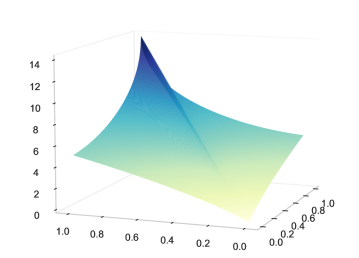
Figure 2: The kernel function $\kappa$. The horizontal axis are $x$- and $y$-axis for the vertex type $\mathcal{S}=[0,1]$, and the vertical axis marks the value $\kappa(x,y)$. The kernel has the following property: 1) clustering behavior. The connection probability is larger between vertices of similar types, demonstrated by the ridge in the diagonal. 2) heterogeneity. Some types have larger connection probabilities in general, shown by the inclination of the surface.

For the bootstrap percolation, we consider a scenario with 10% initially infected vertices. All remaining vertices have a threshold equal to $2$. The initial infection is uniformly distributed over the vertices and independent of the type, i.e.

$$\nu(k,[a,b])=I_{\{k=0\}}\frac{1}{10}\mathinner{\!\left\lvert b-a\right\rvert}+I_{\{k=2\}}\frac{9}{10}\mathinner{\!\left\lvert b-a\right\rvert}.$$ (3.10)

We implement Algorithm 1 to approximate the fixed point $\hat{f}$ that solves $f=\Psi_{\kappa}f$. For this, we choose a neural network with two hidden layers of $20$ nodes each and a hyperbolic tangent activation function. We use the Adam algorithm for parameter optimization which gave the best results. Figure 3 (left) presents the result of the neural network approximation $f^{NN}$ of the fixed point $\hat{f}$ of $\Psi_{\kappa}$. The figure shows values of $f^{NN}$ and $\Psi_{\kappa}^{NN}f^{NN}$. We can see that they perfectly overlap which shows that the algorithm indeed finds the fixed point $\hat{f}$ of $\Psi_{\kappa}$.

We use Algorithm 2 to simulate $M=1000$ samples from the random graph with $n=3000$ vertices and calculate the final number of infected vertices. Note that the randomness only stems from the random skeleton of the graph while conditioned on the realization of the random graph, the percolation process is deterministic. In addition to the total number of infected vertices, we determine the distribution of the types of the infected vertices across all simulations. For this, we split the type space into $L=1000$ subsets of equal length and calculate using Algorithm 2 the number of infected vertices in each of these subsets (analogous to $1000$ bins for a histogram). In Figure 3 (right) we display the curve of $f^{NN}$ together with a scatter plot of the defaulted types. Each point in the scatter plot is a standardized (with respect to the interval length) average of the final fraction of infected vertices with type in the respective subset. We can see that the points lie closely along the $f^{NN}$ curve, which shows that even for random graphs of moderate size the theoretical result of Theorem 2.8 predicts the distribution of the infected vertices very well. By Theorem 2.8, the final fraction of infected vertices is given by $\int_{\mathcal{S}}\hat{f}\mathrm{d}\mu$. Correspondingly, we also calculate $\hat{\tau}\mathrel{\mathop{\ordinarycolon}}=\int_{\mathcal{S}}\hat{f}\mathrm{d}\mu\approx\tau^{NN}\mathrel{\mathop{\ordinarycolon}}=\int_{\mathcal{S}}f^{NN}\mathrm{d}\mu=0.9273$. By Theorem 2.8 for large random graphs, $92.73\%$ of the vertices are expected to be infected at the end of the process, and our simulation well supports this theoretical value with an average of $92.70\%$ infected vertices.

Further, we also expect that the final fraction for each sample of the random graph is close to the theoretical value of $92.73\%$. To visualize how close the final fractions of the samples are to the theoretical value, in Figure 4 (left) we plot the histogram of the final fraction over these $1000$ simulations. We see that the distribution is very narrow, ranging from $90.05\%$ to $94.50\%$, and that it is mostly concentrated around the theoretical value $92.73\%$.

Our result in Theorem 2.8 is asymptotic and is therefore only expected to be a good approximation for random graphs with a large number of vertices $n\rightarrow\infty$. To analyze whether the fraction of infected vertices approaches the theoretical limit as the number of vertices increases, we run simulations for $n$ (numbers of vertices) ranging from $n=200$ to $10000$ in steps of $200$. For each value of $n$, we run $M=1000$ simulations. Figure 4 (right) reports the average simulation result of the final fraction of infected vertices for each $n$ and its $95\%$ confidence band, where the benchmark is the theoretical quantity $\tau^{NN}=0.9273$. We can see from the figure that as $n$ increases, the samples are approaching the theoretical limit, and the $95\%$ confidence band get narrower. This shows that Theorem 2.8 allow us to determine the final fraction of infected vertices already for random networks of moderate size.

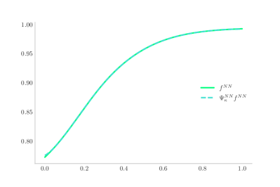
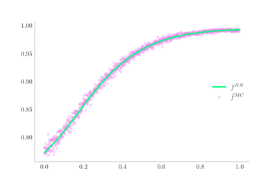
Figure 3: Left: Neural network approximation of the fixed point. Right: Scatter plot of the types of infected vertices. In both pictures, the axis horizontal marks the vertex types $\mathcal{S}=[0,1]$. In the plot on the left hand side, the functions $f^{NN}$ and $\Psi_{\kappa}^{NN}f^{NN}$ perfectly overlap. The perfect alignment of $f^{NN}$ and $\Psi_{\kappa}^{NN}f^{NN}$ implies that $f^{NN}$ is a fixed point of $\Psi_{\kappa}$, which shows that the fixed point algorithm works well. The scatter plot on the right shows the types of infected vertices based on the simulation together with the function $f^{NN}$ which for each type $s\in[0,1]$ by Theorem 2.8 provides the theoretical fraction of infected vertices of this type. The purple points lie closely along the green curve $f_{NN}$ which indicates that the simulation results match the theoretical result of Theorem 2.8 very well.

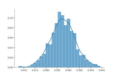
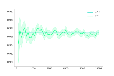
Figure 4: Left: Histogram and density of the final fraction of infected vertices. Right: Mean and confidence interval of the final fraction of infected vertices. The left picture shows the distribution of the final fraction of infected vertices as determined in $M=1000$ simulated random graphs of size $n=3000$. The x-axis marks the final fraction and the y-axis is the proportion. Each blue bar covers an interval and its height shows the proportion of times out of $1000$ simulations that the final fraction falls in this interval. The blue solid smooth curve is the kernel density estimation of the histogram. The right picture plots the mean and $95\%$ confidence interval of the final fraction of infected vertices with $n\in\{200,400,\dots,10000\}$. The number of simulations is $M=1000$. The horizontal blue line marks the theoretical value of the proportion of finally infected vertices as determined by $\hat{\tau}\approx\tau^{NN}\mathrel{\mathop{\ordinarycolon}}=\int_{\mathcal{S}}f^{NN}\mathrm{d}\mu=0.9273$. The green colored line and the band are the average value and the confidence band of the proportion of finally infected vertices. We can see that as $n$ increases, the samples are approaching the theoretical value $\hat{\tau}$ and the confidence interval gets narrower.

Appendix A Graph with A Finite Number of Vertex Types

In this section, we study the graph with finite vertex type introduced in Definition 2.14. We start with a setting with bounded thresholds. For this let $K\in\mathbb{N}$ and we assume that $k_{i}(n)\in[K]\cup\{0\}$ for all $i\in[n]$. We will later extend the model to allow for thresholds in $\mathbb{N}_{0}$. For this reason we will refer to the vertex sequence by $\mathcal{V}_{L,K}^{d}\mathrel{\mathop{\ordinarycolon}}=(\kappa^{d}_{L},\nu,(\bm{s}(n),\bm{k}(n))$ with $K$ explicit in the subscript and to the corresponding graph by $G(n,\mathcal{V}_{L,K}^{d})$.

Instead of exploring the final set of infected vertices $\mathbb{D}(G(n,\mathcal{V}_{L,K}^{d}))$ by generations as described in Section 2, we use a sequential process that results in the same set of infected vertices. The idea is that in each step we only explore the effect on the system triggered by one infected vertex.

For this, at the beginning of each iteration, we uniformly select an infected vertex from the set of unexplored infected vertices. Denote this vertex by $i$. We then explore all edges that vertex $i$ sends to uninfected vertices. We then reduce the threshold value of each receiving vertex by $1$. If the threshold of a receiving vertex reaches $0$, then this vertex is infected and we include it in the set of unexplored infected vertices. Then, after we have updated the threshold of all vertices that received an edge from vertex $i$, we remove the vertex $i$ from the set of unexplored infected vertices. The effect of this vertex has now been explored. We repeat the iteration until there are no more unexplored infected vertices left.

Sequential Exploration Process: To formulate the sequential process, we introduce a "time" index $t\in\mathbb{N}_{0}$ to denote the $t$-th iteration. We first define for $l\in[L]$ and $k\in[K]\cup\{0\}$ the sets

$$U_{k}^{l}(0)\mathrel{\mathop{\ordinarycolon}}=\{i\in\left[n\right]|l_{i}=l,k_{i}(0)=k\}, u_{k}^{l}(0)\mathrel{\mathop{\ordinarycolon}}=|U_{k}^{l}(0)|,$$ (A.1)

where $U_{k}^{l}(0)$ is the (initial) set of type $l$ vertices with threshold $k$. We further denote by $u_{k}^{l}(0)$ their size. Moreover, similar to the regularity condition (2.2), we shall assume the initial proportion $u_{k}^{l}(0)/n$ will converge to a limit $\nu_{k}^{l,*}$:

$$u_{k}^{l}(0)/n\stackrel{{\scriptstyle[}}{{n}}\rightarrow\infty]{p}{\longrightarrow}\nu_{k}^{l,*},$$ (A.2)

where $\sum_{l\in[L]}\sum_{k=0}^{K}\nu_{k}^{l,*}=1$.

Then we keep track of the evolution of the thresholds of the vertices throughout the iterations. For any vertex $i\in[n]$ at round $t$, its threshold $0\leq k_{i}(t)\leq k_{i}(0)$ equals to $k_{i}(0)$ minus the number of edges it has received from explored infected vertices. For each $t\geq 1$ we therefore group vertices by their types and (current) thresholds:

$$U_{k}^{l}(t)\mathrel{\mathop{\ordinarycolon}}=\{i\in\left[n\right]|l_{i}=l,k_{i}(t)=k\}, u_{k}^{l}(t)\mathrel{\mathop{\ordinarycolon}}=|U_{k}^{l}(t)|,$$ (A.3)

We also use $U_{k}(t)$ to denote all the vertices with threshold $k$ at time $t$, and $u_{k}(t)$ to denote their size:

$$U_{k}(t)=\cup_{l\in[L]}U_{k}^{l}(t), u_{k}(t)=\sum_{l\in[L]}u_{k}^{l}(t).$$ (A.4)

Note that after each iteration, we drop the selected and explored infected vertex from the set $U_{0}(t)$, i.e. if $i\in U_{0}(t)$ is selected, then $i\notin U_{0}(t^{\prime})$ for all $t^{\prime}>t$. It holds that $u_{0}(t+1)\geq u_{0}(t)-1$.

The last sets to be tracked are

$$\mathbb{D}(t,G(n,\mathcal{V}_{L,K}^{d})) \mathrel{\mathop{\ordinarycolon}}=\{\text{infected vertices explored up to time }t\},$$ (A.5)

$$\mathbb{D}(G(n,\mathcal{V}_{L,K}^{d})) \mathrel{\mathop{\ordinarycolon}}=\{\text{infected vertices at the end of the process}\}.$$ (A.6)

By the nature of the sequential process we know that $u_{0}(0)\leq|\mathbb{D}(G(n,\mathcal{V}_{L,K}^{d}))|\leq n$.

Therefore, the sequential process is explored in the following manner. At time $t$, we uniformly select an unexplored infected vertex from set $U_{0}(t)$, say vertex $i$, whose threshold is $k_{i}(t)=0$. The probability that the type $l_{i}$ of the uniformly selected vertex $i$ is equal to $l$ is given by $\tfrac{u_{0}^{l}(t)}{u_{0}(t)}$. Then, we explore all the vertices that receive an edge from $i$. If a vertex $j$ with type $l_{j}$ and threshold $k_{j}(t)>0$ receives an edge from $i$, which happens with probability $\kappa(l_{i},l_{j})/n$, then we set $k_{j}(t+1)\mathrel{\mathop{\ordinarycolon}}=k_{j}(t)-1$. Henceforth in the next time step $t+1$, $j$ moves to the set $U_{k_{j}(t)-1}^{l_{j}}(t+1)$ or, equivalently, $U_{k_{j}(t+1)}^{l_{j}}(t+1)$. After all other vertices receiving an edge from $i$ are examined, we consider the vertex $i$ as explored and add it to the set $\mathbb{D}(t,G(n,\mathcal{V}_{L,K}^{d}))=\mathbb{D}(t-1,G(n,\mathcal{V}_{L,K}^{d}))\cup\{i\}$ and remove it for future explorations: $i\notin U_{0}(t+1)$.

Let $h(t)\mathrel{\mathop{\ordinarycolon}}=\left(\{u_{k}^{l}(t)\}_{0\leq k\leq K,1\leq l\leq L}\right)$ describe the state of the entire percolation process at time $t$. According to the algorithm discussed above, for each type $l\in[L]$, we can write down the expected change of the sizes of the vertex sets by the following equations:

$$\mathds{E}[u_{0}^{l}(t+1)-u_{0}^{l}(t)|h(t)] =\left\{-\frac{u_{0}^{l}(t)}{u_{0}(t)}+\left(\sum_{l^{\prime}\in[L]}\frac{u_{0}^{l^{\prime}}(t)}{u_{0}(t)}\frac{\kappa(l^{\prime},l)}{n}\right)u_{1}^{l}(t)\right\},$$ (A.7)

$$\mathds{E}[u_{k}^{l}(t+1)-u_{k}^{l}(t)|h(t)] =\left\{\left(\sum_{l^{\prime}\in[L]}\frac{u_{0}^{l^{\prime}}(t)}{u_{0}(t)}\frac{\kappa(l^{\prime},l)}{n}\right)\left(u_{k+1}^{l}(t)-u_{k}^{l}(t)\right)\right\},\ \forall 1\leq k\leq K-1,$$ (A.8)

$$\mathds{E}[u_{K}^{l}(t+1)-u_{K}^{l}(t)|h(t)] =\left\{-\left(\sum_{l^{\prime}\in[L]}\frac{u_{0}^{l^{\prime}}(t)}{u_{0}(t)}\frac{\kappa(l^{\prime},l)}{n}\right)u_{K}^{l}(t)\right\},$$ (A.9)

and, consequently, the expected change of the sizes of the entire vertex sets across each threshold can be summarized by

$$\mathds{E}[u_{0}(t+1)-u_{0}(t)|h(t)] =\sum_{l\in[L]}\mathds{E}[u_{0}^{l}(t+1)-u_{0}^{l}(t)|h(t)],$$ (A.10)

$$\mathds{E}[u_{k}(t+1)-u_{k}(t)|h(t)] =\sum_{l\in[L]}\mathds{E}[u_{k}^{l}(t+1)-u_{k}^{l}(t)|h(t)],\ \forall 1\leq k\leq K-1,$$ (A.11)

$$\mathds{E}[u_{K}(t+1)-u_{K}(t)|h(t)] =\sum_{l\in[L]}\mathds{E}[u_{K}^{l}(t+1)-u_{K}^{l}(t)|h(t)].$$ (A.12)

To understand the system of equations (A.7), let’s focus on vertices of type $l\in[L]$ and the step from time $t$ to $t+1$. For the first equation, the expected change of the number of infected vertices of type $l$ consists of two parts. First, one already infected vertex is picked up for the sequential exploration with probability $\frac{u_{0}^{l}(t)}{u_{0}(t)}$. This vertex will then drop out and not be in the set $U_{0}^{l}(t+1)$, it will be "explored" in this step, which explains the term $-\frac{u_{0}^{l}(t)}{u_{0}(t)}$. The second, positive term accounts for the newly infected vertices in $U_{1}^{l}(t)$ with a threshold equal to $1$ at the beginning of the step and which get infected because they receive an edge from the currently explored vertex. Because our sequential process can only reduce thresholds by at most one in each time step, only the set $U_{1}^{l}(t)$ contributes to new infections. The probability to select a vertex of type $l^{\prime}$ for exploration in step $t+1$ is $\frac{u_{0}^{l^{\prime}}(t)}{u_{0}(t)}$. Conditioning on the type of the vertex selected being of type $l^{\prime}$, the probability for it to connect to a vertex in the set $U_{1}^{l}(t)$ is $\frac{\kappa(l^{\prime},l)}{n}$. Hence, by summarizing all vertices in $U_{1}^{l}(t)$ we obtain the second term. For threshold $1\leq k\leq K-1$, the change of the set $U_{k}^{l}(t)$ results from vertices in $U_{k+1}^{l}(t)$ which receive an edge from the explored infected vertex and are therefore added to $U_{k}^{l}(t+1)$. The negative term comes from those vertices in $U_{k}^{l}(t)$ that are added to $U_{k-1}^{l}(t+1)$ because they receive an edge from the currently explored vertex. Last, the number of vertices in $U_{K}(t)$ in expectation decreases by the number of vertices in $U_{K}(t)$ that receive an edge from the vertex that is currently being explored.

Approximation with ODEs: We will approximate the components of $h(t)/n$ in the system (A.7) using the well-known method proposed in Wormald [27] by the vector $\left(\{\nu_{k}^{l}(\tau)\}_{\begin{subarray}{c}0\leq k<\infty\\ 1\leq l\leq L\end{subarray}}\right)$, where $\nu_{k}^{l}(\tau)\mathrel{\mathop{\ordinarycolon}}[0,1]\rightarrow[0,1]$, that solves the following system of ordinary differential equations:

$$\frac{\mathrm{d}\nu_{0}^{l}(\tau)}{\mathrm{d}\tau} =-\frac{\nu_{0}^{l}(\tau)}{\nu_{0}(\tau)}+\left(\sum_{l^{\prime}\in[L]}\frac{\nu_{0}^{l^{\prime}}(\tau)}{\nu_{0}(\tau)}\kappa(l^{\prime},l)\right)\nu_{1}^{l}(\tau),$$ (A.13)

$$\frac{\mathrm{d}\nu_{k}^{l}(\tau)}{\mathrm{d}\tau} =\left(\sum_{l^{\prime}\in[L]}\frac{\nu_{0}^{l^{\prime}}(\tau)}{\nu_{0}(\tau)}\kappa(l^{\prime},l)\right)\left(\nu_{k+1}^{l}(\tau)-\nu_{k}^{l}(\tau)\right),\ \forall 1\leq k\leq K-1,$$ (A.14)

$$\frac{\mathrm{d}\nu_{K}^{l}(\tau)}{\mathrm{d}\tau} =-\left(\sum_{l^{\prime}\in[L]}\frac{\nu_{0}^{l^{\prime}}(\tau)}{\nu_{0}(\tau)}\kappa(l^{\prime},l)\right)\nu_{K}^{l}(\tau),$$ (A.15)

with initial condition

$$\nu_{k}^{l}(0)=u_{k}^{l}(0)/n,\ \forall k\in[K]\cup\{0\}.$$ (A.16)

The solution for the system (A.13) is given by

$$\nu_{0}^{l}(\tau) =-\beta^{l}(\tau)+\nu_{0}^{l}(0)+\sum_{k^{\prime}=1}^{K}\nu_{k^{\prime}}^{l}(0)\left(1-\sum_{k^{\prime\prime}=0}^{k^{\prime}-1}p(k^{\prime\prime},\lambda^{l}(\tau))\right),$$ (A.17)

$$\nu_{k}^{l}(\tau) =\sum_{k^{\prime}=k}^{K}\nu_{k^{\prime}}^{l}(0)p(k^{\prime}-k,\lambda^{l}(\tau)),\ \forall 1\leq k\leq K-1,$$ (A.18)

$$\nu_{K}^{l}(\tau) =\nu_{K}^{l}(0)p(0,\lambda^{l}(\tau)),$$ (A.19)

where

$$\beta^{l}(\tau)\mathrel{\mathop{\ordinarycolon}}=\int_{0}^{\tau}\frac{\nu_{0}^{l}(s)}{\nu_{0}(s)}\mathrm{d}s, \lambda^{l}(\tau)\mathrel{\mathop{\ordinarycolon}}=\sum_{l^{\prime}\in[L]}\kappa(l^{\prime},l)\beta^{l^{\prime}}(\tau), p(k,\lambda)\mathrel{\mathop{\ordinarycolon}}=\frac{\lambda^{k}}{k!}\mathrm{e}^{-\lambda}.$$ (A.20)

The following lemma asserts the condition for the differential equation system (A.13) to approximate the system (A.7).

Lemma A.1.

1. For $\delta>0$, the equation system (A.13) fulfills a Lipschitz condition on the domain

$$\mathcal{D}_{\delta}=\left\{\left(\tau,\{\nu_{k}^{l}\}_{0\leq k\leq K,1\leq l\leq L}\right)\in\mathcal{R}^{K+L+2}\mathrel{\mathop{\ordinarycolon}}0<\tau<1,0<\nu_{k}^{l}(\tau)<1,\sum_{l\in[L]}\nu_{0}^{l}(\tau)>\delta\right\}.$$ (A.21)

2. There exist functions $\omega=\omega(n)$ and $\gamma=\gamma(n)$ with $\gamma\rightarrow\infty$ as $n\rightarrow\infty$ and $\gamma^{4}\log n<\omega<n^{2/3}/\gamma$ such that

$$\mathds{P}\left(\mathinner{\!\left\lvert u_{k}^{l}(t+1)-u_{k}^{l}(t)\right\rvert}>\frac{\sqrt{\omega}}{\gamma^{2}\sqrt{\log n}}|h(t)\right)=o(n^{-3})$$ (A.22)

for all $k\in[K]\cup\{0\}$ and $l\in[L]$.

Proof.

For 1. Let $f_{k}^{l}\mathrel{\mathop{\ordinarycolon}}=f_{k}^{l}(\tau,\{\nu_{k}^{l}\}_{0\leq k\leq K,1\leq l\leq L})\mathrel{\mathop{\ordinarycolon}}=\frac{\mathrm{d}\nu_{0}^{l}}{\mathrm{d}\tau}$, we take partial derivatives of system (A.13) with respect to $\{\nu_{k}^{l}\}$:

$$\frac{\partial f_{0}^{l}}{\partial\nu_{0}^{l}} =-\frac{1}{\nu_{0}}(1-\alpha^{l})+\frac{\nu_{1}^{l}}{\nu_{0}^{l}}\left(\kappa(l,l)-\sum_{l^{\prime}\in[L]}\kappa(l^{\prime},l)\right),$$ (A.23)

$$\frac{\partial f_{0}^{l}}{\partial\nu_{0}^{l^{\prime}}} =-\frac{1}{\nu_{0}}\alpha^{l}+\frac{\nu_{1}^{l}}{\nu_{0}^{l}}\left(\kappa(l^{\prime},l)-\sum_{l^{\prime\prime}\in[L]}\kappa(l^{\prime\prime},l)\right),\ l\neq l^{\prime},$$ (A.24)

$$\frac{\partial f_{0}^{l}}{\partial\nu_{1}^{l}} =\sum_{l^{\prime}\in[L]}\alpha^{l^{\prime}}\kappa(l^{\prime},l),$$ (A.25)

$$\frac{\partial f_{k}^{l}}{\partial\nu_{1}^{l}} =\left(\frac{\nu_{k+1}^{l}}{\nu_{0}^{l}}-\frac{\nu_{k}^{l}}{\nu_{0}^{l}}\right)\left(\kappa(l^{\prime},l)-\sum_{l^{\prime\prime}\in[L]}\alpha^{l^{\prime\prime}}\kappa(l^{\prime\prime},l)\right),\ \forall 1\leq k\leq K-1,$$ (A.26)

$$\frac{\partial f_{k}^{l}}{\partial\nu_{k+1}^{l}} =\sum_{l^{\prime}\in[L]}\alpha^{l^{\prime}}\kappa(l^{\prime},l),\ \forall 1\leq k\leq K-1,$$ (A.27)

$$\frac{\partial f_{k}^{l}}{\partial\nu_{k}^{l}} =-\sum_{l^{\prime}\in[L]}\alpha^{l^{\prime}}\kappa(l^{\prime},l),\ \forall 1\leq k\leq K-1,$$ (A.28)

$$\frac{\partial f_{K}^{l}}{\partial\nu_{K}^{l}} =-\frac{\nu_{K}^{l}}{\nu_{0}^{l}}\left(\kappa(l^{\prime},l)-\sum_{l^{\prime\prime}\in[L]}\alpha^{l^{\prime\prime}}\kappa(l^{\prime\prime},l)\right),$$ (A.29)

$$\frac{\partial f_{K}^{l}}{\partial\nu_{K}^{l}} =-\sum_{l^{\prime}\in[L]}\alpha^{l^{\prime}}\kappa(l^{\prime},l).$$ (A.30)

Notice the fact that $\forall 1\leq l,l^{\prime}\leq L$, $0\leq\alpha^{l}\leq 1$ and $\kappa(l^{\prime},l)$ is finite, and that we only need to consider $0<\tau<1$ and $0<\nu_{k}^{l}<1$ for the system (A.13), another condition we need is just $\nu_{0}>\delta$.

For 2. As in Detering et al. [13], choose $\omega(n)=B^{2}n^{25/48}$ with $B>0$ constant and $\gamma(n)=n^{1/8}$, then

$$\frac{\sqrt{\omega}}{\gamma^{2}\sqrt{\log n}}=\frac{Bn^{1/96}}{\sqrt{\log n}}.$$ (A.31)

A rough bound can be found by

$$\mathds{P}\left(\mathinner{\!\left\lvert u_{k}^{l}(t+1)-u_{k}^{l}(t)\right\rvert}\geq d|h(t)\right)\leq n\binom{n-1}{d}\left(\frac{M}{n}\right)^{d}\leq n\frac{M^{2d}}{d!}$$ (A.32)

where $M\mathrel{\mathop{\ordinarycolon}}=\sup_{l\in[L]}\sum_{l^{\prime}\in[l]}\kappa(l^{\prime},l)$. Noting that $d!\geq n^{5}M^{2d}$ for $d\geq n^{1/100}$ and large $n$ completes the proof. ∎

Therefore by Wormald [27], we can approximate the system (A.7) by

$$u_{k}^{l}(t)=n\nu_{k}^{l}(t/n)+o(n),\ \forall 0\leq k\leq K,\ 1\leq l\leq L,$$ (A.33)

almost surely within the domain $\mathcal{D}_{\delta}$ where $0<t/n<1$ and $\sum_{l\in[L]}\nu_{0}^{l}(t/n)>\delta$.

A heuristic interpretation of the solution (A.17) is as follows: At the time $\tau$ of the percolation, for a vertex of type $l\in[L]$, its degree to the set of infected vertices is approximately Poisson distributed with parameter $\lambda^{l}(\tau)$. Note that $p(k,\lambda)$ is exactly defined in the form of the probability mass function of a Poisson random variable with parameter $\lambda$. In other words, for $0\leq k^{\prime}\leq k\leq K$, a vertex of type $l$ and initial threshold of $k$ has probability $p(k-k^{\prime},\lambda^{l}(\tau))$ to be translated to a threshold of $k^{\prime}$ at time $\tau$. Therefore, at time $\tau$, the fraction of vertices of type $l$ and threshold $k$ is summarized over the fractions of all other vertices with initially threshold $k^{\prime}\geq k$ that receive exactly $k^{\prime}-k$ infectious connections.

We are interested in the time $\hat{t}$ when the sequential exploration stops, i.e. $U(\hat{t})=\emptyset$ and $U(t)\neq\emptyset$ for $t<\hat{t}$. It is clear that $\hat{t}=|\mathbb{D}(G(n,\mathcal{V}_{L,K}^{d}))|$ by the nature of the exploration process. Because the approximation only holds in $\mathcal{D}_{\delta}$ and thus stops to hold before the sequential exploration comes to the end, we shall first study the time when the number of unexplored infected vertices reach a small proportion $\delta>0$ and show that this time converges as $\delta$ goes to $0$. Then, in the next step, we derive a condition that ensures that when the fraction of unexplored infected vertices reduces to zero, the actually process ends and it can not rebound and trigger new infections. That is, let $\hat{t}^{\delta}$ be the first time when $u_{0}(\hat{t}^{\delta})/n\leq\delta$, then we need to show that $\hat{t}/n$ converges and that $\hat{t}^{\delta}/n$ converges to $\hat{t}/n$ as $\delta$ goes to zero.

Thus, for the ODE system (A.33), we define the two corresponding times $\widehat{\tau}$ and $\widehat{\tau}^{\delta}$ as follows:

Definition A.2.

We denote by $\widehat{\tau}$ the first time when all the $\{\nu_{0}^{l}\}$, $l\in[L]$ in the solution to the ODE system (A.33) reach zero. In addition we denote by $\widehat{\tau}^{\delta}$ the first time when $\sum_{l=1}^{L}\nu_{0}^{l}$, $l\in[L]$ reaches a small positive $\delta$:

$$\widehat{\tau}\mathrel{\mathop{\ordinarycolon}}=\inf\left\{\tau\mathrel{\mathop{\ordinarycolon}}\left\{\nu_{0}^{l}(\tau)\right\}_{1\leq l\leq L}=\mathbf{0}\right\}, \widehat{\tau}^{\delta}\mathrel{\mathop{\ordinarycolon}}=\inf\left\{\tau\mathrel{\mathop{\ordinarycolon}}\sum_{l\in[L]}\nu_{0}^{l}(\tau)=\delta\right\}.$$ (A.34)

Note that the solution (A.17) is not explicit due to the integral term $\beta^{l}(\tau)$. Observe that $\beta^{l}(\tau)\in\left[0,1\right]$ and $\beta^{l}$ is monotonically increasing in $\tau\in[0,\widehat{\tau}]$ and that $\sum_{l\in[L]}\beta^{l}(\tau)=\tau$, which we will use later.

Now, with a little abuse of notation, define the functions $\nu\mathrel{\mathop{\ordinarycolon}}\mathbb{R}^{L}\rightarrow[0,1]$ and $\lambda\mathrel{\mathop{\ordinarycolon}}\mathbb{R}^{L}\rightarrow\mathbb{R}$ by

$$\nu_{0}^{l}(\mathbf{z}) =-z^{l}+\sum_{k^{\prime}=0}^{K}\nu_{k^{\prime}}^{l}(\mathbf{0})\left(1-\sum_{k^{\prime\prime}=0}^{k^{\prime}-1}p(k^{\prime\prime},\lambda^{l}(\mathbf{z}))\right),$$ (A.35)

$$\nu_{k}^{l}(\mathbf{z}) =\sum_{k^{\prime}=k}^{K}\nu_{k^{\prime}}^{l}(\mathbf{0})p(k^{\prime}-k,\lambda^{l}(\mathbf{z})),\ \forall 1\leq k\leq K-1,$$ (A.36)

$$\nu_{K}^{l}(\mathbf{z}) =\nu_{K}^{l}(\mathbf{0})p(0,\lambda^{l}(\mathbf{z})),$$ (A.37)

where

$$\mathbf{z}\mathrel{\mathop{\ordinarycolon}}=\left\{z^{l}\right\}_{1\leq l\leq L}\in\left[0,1\right]^{L}, \lambda^{l}(\mathbf{z})\mathrel{\mathop{\ordinarycolon}}=\sum_{l^{\prime}\in[L]}\kappa(l^{\prime},l)z^{l^{\prime}}.$$ (A.38)

The partial derivative of $\nu_{0}^{l}(\mathbf{z})$ is given by

$$\frac{\partial\nu_{0}^{l}(\mathbf{z})}{\partial z^{l^{\prime}}} =-\delta_{l,l^{\prime}}+\kappa(l^{\prime},l)\nu_{1}^{l}(\mathbf{z})$$ (A.39)

where $\delta_{l,l^{\prime}}$ is the Kronecker delta.

Define now

$$\mathcal{Z}_{0}\mathrel{\mathop{\ordinarycolon}}=\left\{\mathbf{z}\mathrel{\mathop{\ordinarycolon}}\bm{\nu_{0}}(\mathbf{z})=\mathbf{0}\right\}, \mathcal{Z}_{\delta}\mathrel{\mathop{\ordinarycolon}}=\left\{\mathbf{z}\mathrel{\mathop{\ordinarycolon}}\sum_{l\in[L]}\nu_{0}^{l}(\mathbf{z})=\delta\right\},$$ (A.40)

$$\widehat{\mathbf{z}}\mathrel{\mathop{\ordinarycolon}}=\min\left\{\mathcal{Z}_{0}\right\}, \widehat{\mathbf{z}}^{\delta}\mathrel{\mathop{\ordinarycolon}}=\min\left\{\mathcal{Z}_{\delta}\right\}.$$ (A.41)

It is easy to verify the existence of the last two component-wise minimal $\widehat{\mathbf{z}}$ and $\widehat{\mathbf{z}}^{\delta}$ by rewriting the first equation of (A.35) as a fixed point problem analogous to equation (2.4), using properties of functions $\nu^{l}_{0}$, and applying the Knaster-Tarski theorem. Therefore, it holds that

$$\sum_{l\in[L]}\widehat{z}^{l}=\min_{\mathbf{z}\in\mathcal{Z}_{0}}\left\{\sum_{l\in[L]}z^{l}\right\}, \sum_{l\in[L]}\widehat{z}^{\delta,l}=\min_{\mathbf{z}\in\mathcal{Z}_{\delta}}\left\{\sum_{l\in[L]}z^{l}\right\}.$$ (A.42)

Proposition A.3 (First joint zeros).

For $\widehat{\tau}$ and $\widehat{\tau}^{\delta}$ as defined in equation (A.34), and $\widehat{\mathbf{z}}$ and $\widehat{\mathbf{z}}^{\delta}$ defined in equation (A.40) the following holds true:

$$\bm{\beta}(\widehat{\tau})=\widehat{\mathbf{z}}, \widehat{\tau}=\sum_{l\in[L]}\widehat{z}^{l}, \bm{\beta}(\widehat{\tau}^{\delta})\geq\widehat{\mathbf{z}}^{\delta}, \widehat{\tau}^{\delta}\geq\sum_{l\in[L]}\widehat{z}^{\delta,l}.$$ (A.43)

Proof.

It is easy to see the last two inequalities that $\bm{\beta}(\widehat{\tau}^{\delta})\geq\widehat{\mathbf{z}}^{\delta}$ because $\bm{\beta}(\widehat{\tau}^{\delta})\in\mathcal{Z}_{\delta}$ and by the definition of $\widehat{\mathbf{z}}^{\delta}$. It follows that $\widehat{\tau}^{\delta}=\sum_{l\in[L]}\beta^{l}(\widehat{\tau}^{\delta})\geq\sum_{l\in[L]}\widehat{z}^{\delta,l}$. For the first two equalities, we have $\bm{\beta}(\widehat{\tau})\geq\widehat{\mathbf{z}}$ as $\bm{\beta}(\widehat{\tau})\in\mathcal{Z}_{0}$ and by the definition of $\widehat{\mathbf{z}}$. To show the equality by contradiction, suppose $\bm{\beta}(\widehat{\tau})>\widehat{\mathbf{z}}$. Since $\bm{\beta}$ is continuous and non-decreasing in $[0,\widehat{\tau}]$ and $\bm{\beta}(0)=\bm{0}$, there exists $\bar{\tau}<\widehat{\tau}$ when a certain type $l\in[L]$ first reaches $\beta^{l}(\bar{\tau})=\widehat{z}^{l}$ and we have $\bm{\beta}(\bar{\tau})\leq\mathbf{\widehat{z}}$. Then, if $\beta^{l^{\prime}}(\bar{\tau})=\widehat{z}^{l^{\prime}}$ for all $l^{\prime}\in[L]$ and $l^{\prime}\neq l$, then $\bm{\nu_{0}}(\bm{\beta}(\bar{\tau}))=\bm{\nu_{0}}(\mathbf{\widehat{z}})=\mathbf{0}$, which contradicts with the definition of the first zero $\widehat{\tau}$. Hence, there should exist at least one $l^{\prime}\in[L],\ l^{\prime}\neq l$ such that $\beta^{l^{\prime}}(\bar{\tau})<\widehat{z}^{l^{\prime}}$. However, with $\tfrac{\partial\nu_{0}^{l}(\mathbf{z})}{\partial z^{l^{\prime}}}>0$ for all $l^{\prime}\neq l$, we have that $\nu_{0}^{l}(\bm{\beta}(\bar{\tau}))<\nu_{0}^{l}(\mathbf{\widehat{z}})=0$, which contradicts with $\nu_{0}^{l}(\tau)\geq 0$ for $0<\tau<\widehat{\tau}$. Therefore, we conclude that $\bm{\beta}(\widehat{\tau})=\widehat{\mathbf{z}}$ and $\widehat{\tau}=\sum_{l\in[L]}\beta^{l}(\widehat{\tau})=\sum_{l\in[L]}\widehat{z}^{l}$. ∎

Remaining Process: The approximation system (A.35) works in the domain $\mathcal{D}_{\delta}$ before the process reaches $\widehat{\tau}^{\delta}$ at which point there is still a proportion $\delta$ of infected vertices left that is not yet explored. We want to know whether the percolation arising from these remaining $\delta n$ vertices comes to the end soon or whether they still trigger a large number of additional infections. Thus, we study now the process triggered by the remaining small proportion $\delta$ of infected vertices, which we call the remaining process. We explore the remaining process starting from the step $\lfloor\widehat{\tau}^{\delta}n\rfloor$ by generations instead of the sequential procedure used so far. Then, we show that, under an appropriate condition, the proportion of infected vertices in the remaining process will converge to zero.

For this we group the remaining uninfected vertices at step $\lfloor\widehat{\tau}^{\delta}n\rfloor$ into weak vertices and strong vertices by their threshold as follows: Let

$$W^{l}\mathrel{\mathop{\ordinarycolon}}=U_{1}^{l}(\lfloor\widehat{\tau}^{\delta}n\rfloor), W\mathrel{\mathop{\ordinarycolon}}=\bigcup_{l\in[L]}W^{l}$$ (A.44)

denote sets of weak type $l$ vertices which have threshold equal to $1$, and their union set of all weak vertices; and

$$S^{l}\mathrel{\mathop{\ordinarycolon}}=\bigcup_{k=2}^{K}U_{k}^{l}(\lfloor\widehat{\tau}^{\delta}n\rfloor), S\mathrel{\mathop{\ordinarycolon}}=\bigcup_{l\in[L]}S^{l}$$ (A.45)

denote sets of strong type $l$ vertices which have threshold greater or equal to $2$, and their union set of all "strong" vertices. To track the iterative exploration, we use subscript $j\in\mathbb{N}$ for the $j$-th round of iteration of our exploration process. Let $U_{0}^{l}\mathrel{\mathop{\ordinarycolon}}=U_{0}^{l}(\lfloor\widehat{\tau}^{\delta}n\rfloor)$ denote the "initial" set of infected vertices of type $l\in[L]$ in the remaining process; $W_{j}^{l}$ and $S_{j}^{l}$ denote the type $l$ "weak" vertices and "strong" vertices in the $j$-th round of exploration.

Our remaining process is explored as follows: in the first round, we examine all the "weak" vertices and "strong" vertices that are infected by vertices in $U_{0}$, hence we obtain corresponding sets $W_{1}^{l}$, $S_{1}^{l}$, $W_{1}\cup S_{1}$; in the second round, we examine the newly infected vertices $W_{2}^{l}$, $S_{2}^{l}$, $W_{2}\cup S_{2}$, which can only be infected by the previous sets $W_{1}^{l}$ and $S_{1}^{l}$; and so on. Iterating via such exploration, we obtain the set of all the infected vertices in the remaining process $\bigcup_{j=1}^{\infty}W_{j}\cup S_{j}$. Here we first state a lemma on the derivative condition at $\widehat{\mathbf{z}}$ which leads to the Proposition A.5 for $n^{-1}|\bigcup_{j=1}^{\infty}W_{j}\cup S_{j}|$ to converge to zero.

Lemma A.4.

Let $\widehat{\mathbf{z}}$ as defined in (A.40). If for some $\epsilon>0$ and some some direction $\{w^{l}\}_{1\leq l\leq L}\in\{w^{l}>0,\sum_{l\in[L]}w^{l}\leq 1\}$, we have

$$\sum_{l^{\prime}\in[L]}w^{l^{\prime}}\frac{\partial\nu_{0}^{l}(\widehat{\mathbf{z}})}{\partial z^{l^{\prime}}}<-\epsilon,\ \forall 1\leq l\leq L,$$ (A.46)

then there exists some $\delta^{*}>0$ and $0<\epsilon^{*}<\epsilon$ such that for all $0<\delta<\delta^{*}$ it holds that

$$\sum_{l^{\prime}\in[L]}w^{l^{\prime}}\frac{\partial\nu_{0}^{l}(\widehat{\mathbf{z}}^{\delta})}{\partial z^{l^{\prime}}}<-\epsilon^{*},\ \forall 1\leq l\leq L.$$ (A.47)

where $\widehat{\mathbf{z}}^{\delta}$ is as defined in (A.40).

Proof.

Note that $\mathbf{z}^{\delta}\leq\widehat{\mathbf{z}}$. For some positive $\bm{\delta}\in\mathbb{R}^{L}$, let $\mathbf{z}^{\delta}=\widehat{\mathbf{z}}-\bm{\delta}$, plug in the Derivative (A.39) into the l.h.s of the inequality (A.47), and insert $\lambda$ and $p(k,\lambda)$ defined in equation (A.17) and (A.35), we have

$$\sum_{l^{\prime}\in[L]}w^{l^{\prime}}\frac{\partial\nu_{0}^{l}(\widehat{\mathbf{z}})}{\partial z^{l^{\prime}}} =\sum_{l^{\prime}\in[L]}w^{l^{\prime}}\kappa(l^{\prime},l)\nu_{1}^{l}(\widehat{\mathbf{z}}-\bm{\delta})$$ (A.48)

$$=\sum_{l^{\prime}\in[L]}w^{l^{\prime}}\kappa(l^{\prime},l)\sum_{k^{\prime}=k}^{K}\nu_{k^{\prime}}^{l}(\mathbf{0})p(k^{\prime}-k,\lambda^{l}(\widehat{\mathbf{z}}-\bm{\delta}))$$ (A.49)

$$\leq\sum_{l^{\prime}\in[L]}w^{l^{\prime}}\kappa(l^{\prime},l)\sum_{k^{\prime}=k}^{K}\nu_{k^{\prime}}^{l}(\mathbf{0})p(k^{\prime}-k,\lambda^{l}(\widehat{\mathbf{z}}))\mathrm{e}^{-\lambda^{l}(\bm{\delta})}$$ (A.50)

$$\leq\sum_{l^{\prime}\in[L]}w^{l^{\prime}}\frac{\partial\nu_{0}^{l}(\widehat{\mathbf{z}})}{\partial z^{l^{\prime}}}\min_{l\in[L]}\mathrm{e}^{-\lambda^{l}(\bm{\delta})}$$ (A.51)

$$\leq-\epsilon\min_{l\in[L]}\mathrm{e}^{-\lambda^{l}(\bm{\delta})}$$ (A.52)

$$\leq-\epsilon\min_{l\in[L]}\mathrm{e}^{-\lambda^{l}(\bm{\delta}^{*})},$$ (A.53)

where $\mathbf{0}<\bm{\delta}<\bm{\delta}^{*}$. Let $\epsilon^{*}=-\epsilon\min_{l\in[L]}\mathrm{e}^{-\lambda^{l}(\bm{\delta}^{*})}$ and the result follows. ∎

Proposition A.5 (Convergence of remaining process).

If condition A.46 of Lemma A.4 holds, then

$$n^{-1}\mathinner{\!\left\lvert\bigcup_{j=1}^{\infty}W_{j}\cup S_{j}\right\rvert}\stackrel{{\scriptstyle[}}{{\delta}}\rightarrow 0]{p}{\rightarrow}0.$$ (A.54)

Proof.

Apply Lemma A.4, and choose a small $\delta^{*}>0$, then for any $0<\delta<\delta^{*}$, it holds

$$\sum_{l^{\prime}\in[L]}w^{l^{\prime}}\frac{\partial\nu_{0}^{l}(\widehat{\mathbf{z}}^{\delta})}{\partial z^{l^{\prime}}}<-\epsilon^{*},\ \forall 1\leq l\leq L,$$ (A.55)

for some small $0<\epsilon^{*}<\epsilon$. Then, for the fixed $\{w^{l}\}_{1\leq l\leq L}$, plugging the derivative (A.39) into the above inequality yields

$$\sum_{l^{\prime}\in[L]}w^{l^{\prime}}\kappa(l^{\prime},l)\nu_{1}^{l}(\widehat{\mathbf{z}}^{\delta})<c_{1}^{l}w^{l}<w^{l}-\epsilon^{*},$$ (A.56)

$$\sum_{l\in[L]}\sum_{l^{\prime}\in[L]}w^{l^{\prime}}\kappa(l^{\prime},l)\nu_{1}^{l}(\widehat{\mathbf{z}}^{\delta})<\sum_{l\in[L]}c_{1}^{l}w^{l}<c_{1}\sum_{l\in[L]}w^{l}\leq c_{1},$$ (A.57)

where $0<c_{1}^{l}<1$ and $c_{1}=\max_{l}c_{1}^{l}$ are constants not depending on $\delta$.

Next, for any other $0<\delta^{\prime}<\delta^{*}$ and the fixed direction $\mathbf{w}$, as $\nu_{0}^{l}$ decreases with $\delta$ we are able to choose $0<\delta<\delta^{\prime}$ such that

$$\nu_{1}^{l}(\widehat{\mathbf{z}}^{\delta})<w^{l}\delta^{\prime},\ \forall l\in[L].$$ (A.58)

Then, we use induction to show that

$$\mathds{E}\left[|W_{j}|\right]\leq c_{1}c^{j-1}\delta^{\prime}n, \mathds{E}\left[|S_{j}|\right]\leq c_{2}c^{j-1}\delta^{\prime}n,$$ (A.59)

where $0<c_{1}<c<1$, $c_{2}=c-c_{1}$. First, for $j=1$, fix an infected vertex $x\in U_{0}^{l^{\prime}}$ and a "weak" vertex $y\in W^{l}$, we write the connection probability as

$$p_{l^{\prime}l} \mathrel{\mathop{\ordinarycolon}}=\mathds{P}\left\{E_{xy}=1|x\in U_{0}^{l^{\prime}},y\in W^{l}\right\}=\frac{\kappa(l^{\prime},l)}{n}.$$ (A.60)

Then, the probability that the "weak" vertex $y$ is infected is

$$p_{l} \mathrel{\mathop{\ordinarycolon}}=\mathds{P}\left\{\cup_{l^{\prime}=1}^{L}\cup_{x\in U_{0}^{l^{\prime}}}\{E_{xy}=1\}|x\in U_{0},y\in W^{l}\right\}\leq\sum_{l^{\prime}\in[L]}\frac{\kappa(l^{\prime},l)}{n}|U_{0}^{l^{\prime}}|.$$ (A.61)

Recalling that the size of infected vertices at step $\lfloor\hat{\tau}^{\delta}n\rfloor$ is $|U_{0}|\leq\delta n$ and $|W^{l}|=|U_{1}^{l}(\lfloor\widehat{\tau}^{\delta}n\rfloor)|$, we obtain the following inequality for the expected size of "weak" vertices infected in the first round:

$$\mathds{E}\left[|W_{1}|\right] \leq\mathds{E}\left[\sum_{x,y}I_{\{E_{xy}=1\}}|x\in U_{0},y\in W\right]$$ (A.62)

$$\leq\sum_{l\in[L]}|W^{l}|p_{l}$$ (A.63)

$$=\sum_{l\in[L]}\sum_{l^{\prime}\in[L]}\frac{\kappa(l^{\prime},l)}{n}|W^{l}||U_{0}^{l^{\prime}}|$$ (A.64)

$$\leq n\delta^{\prime}\sum_{l\in[L]}c_{1}^{l}w^{l}$$ (A.65)

$$\leq c_{1}\delta^{\prime}n,$$ (A.66)

where we use inequalities (A.56) and (A.58).

For "strong" vertices, we first calculate the probability that a fixed vertex $y\in S$ receives edges from at least two infected vertices $x_{1}\in U_{0}^{l^{\prime}}$ and $x_{2}\in U_{0}^{l^{\prime\prime}}$ which is

$$p(x_{1},x_{2},y,l^{\prime},l^{\prime\prime})\mathrel{\mathop{\ordinarycolon}} =\mathds{P}\left\{\{E_{x_{1}y}=1,E_{x_{2}y}=1\}|x_{1}\in U_{0}^{l^{\prime}},x_{2}\in U_{0}^{l^{\prime\prime}},y\in S\right\}$$ (A.67)

$$=\sum_{l\in[L]}\frac{\kappa(l^{\prime},l)\kappa(l^{\prime\prime},l)}{n^{2}}|S^{l}|.$$ (A.68)

The expected number of "strong" vertices infected in the first round can be bounded as follows:

$$\mathds{E}\left[|S_{1}|\right] \leq\mathds{E}\left[I_{\{E_{x_{1}y}=1,E_{x_{2}y}=1\}}|x_{1}\in U_{0},x_{2}\in U_{0},y\in S\right]$$ (A.69)

$$\leq\frac{1}{2}\sum_{l^{\prime}\in[L]}|U_{0}^{l^{\prime}}|\sum_{l^{\prime\prime}\in[L]}|U_{0}^{l^{\prime\prime}}|p(x_{1},x_{2},y,l^{\prime},l^{\prime\prime})$$ (A.70)

$$\leq\frac{M^{2}}{2n^{2}}|U_{0}|^{2}|S|$$ (A.71)

$$\leq\frac{1}{2}M^{2}\delta^{\prime 2}n$$ (A.72)

$$\leq c_{2}\delta^{\prime}n,$$ (A.73)

where $M=\max_{l^{\prime}}\{\sum_{l\in[L]}\kappa(l^{\prime},l)\}$ by Assumption 2.2.

Next, by induction, assume inequality (A.59) holds for $j=i,i\geq 1$, then for $j=i+1$ we have

$$\mathds{E}\left[|W_{i+1}|\right] \leq\mathds{E}\left[I_{\{E_{xy}=1\}}|x\in W_{i}\cup S_{i},y\in W\backslash\cup_{j=1}^{i}W_{i}\right]$$ (A.74)

$$\leq\mathds{E}\left[I_{\{E_{xy}=1\}}|x\in W_{i}\cup S_{i},y\in W\right]$$ (A.75)

$$\leq\sum_{l\in[N(L)]}\sum_{l^{\prime}\in[L]}\frac{\kappa(l^{\prime},l)}{n}|W^{l}|\mathds{E}\left[|(W_{i}\cup S_{i})^{l^{\prime}}|\right]$$ (A.76)

$$\leq c_{1}c^{i}m\delta^{\prime}n,$$ (A.77)

$$\mathds{E}\left[|S_{i+1}|\right] \leq\mathds{E}\left[I_{\{E_{x_{1}y}=1,E_{x_{2}y}=1\}}|x_{1}\in W_{i}\cup S_{i},x_{2}\in W_{i}\cup S_{i},y\in\backslash\cup_{j=1}^{i}S_{i}\right]$$ (A.78)

$$\leq\frac{\kappa^{2}}{2n^{2}}\mathds{E}\left[|(W_{i}\cup S_{i})|\right]^{2}|S|$$ (A.79)

$$\leq\frac{1}{2}\kappa^{2}c^{2i}\delta^{\prime 2}n$$ (A.80)

$$\leq c_{2}c^{i}\delta^{\prime}n.$$ (A.81)

Applying inequalities (A.74) and recalling that $0<c=c_{1}+c_{2}<1$, for any $a>0$ we can use the Markov inequality which leads to the result (A.54):

$$\mathds{P}\left\{\frac{|\bigcup_{j=1}^{\infty}W_{j}\cup S_{j}|}{n}>a\right\} \leq a^{-1}\mathds{E}\left[\frac{|\bigcup_{j=1}^{\infty}W_{j}\cup S_{j}|}{n}\right]$$ (A.82)

$$\leq a^{-1}\sum_{j=1}^{\infty}\mathds{E}\left[\frac{|W_{j}\cup S_{j}|}{n}\right]$$ (A.83)

$$\leq a^{-1}\sum_{j=1}^{\infty}(c_{1}+c_{2})c^{j}\delta^{\prime}$$ (A.84)

$$\leq\frac{c\delta^{\prime}}{(1-c)a}.$$ (A.85)

∎

Theorem A.6 (Final fraction of infected vertices for graph with finite vertex type).

If the condition A.46 as in Lemma A.4 holds for the graph with finite vertex type $G(n,\mathcal{V}_{L}^{d})$ (A.7), then we have

$$n^{-1}|\mathbb{D}(G(n,\mathcal{V}_{L,K}^{d}))|\xrightarrow[n\rightarrow\infty]{p}\widehat{\tau}$$ (A.86)

where $\widehat{\tau}$ is the first zero defined in equation (A.34).

Remark A.7.

If condition (A.46) does not hold, we still have

$$n^{-1}\mathbb{D}(G(n,\mathcal{V}_{L,K}^{d}))|\geq\widehat{\tau}.$$ (A.87)

Proof.

The ODE approximation (A.13) applies in domain $\mathcal{D}_{\delta}$ until $\widehat{\tau}^{\delta}$ is reached. Thus, at $\widehat{\tau}^{\delta}$, the number of infected vertices which have been explored is $n\widehat{\tau}^{\delta}$; meanwhile, the number of unexplored infected vertices is $u_{0}(n\widehat{\tau}^{\delta})=n\delta+o(n)$ almost surely, by equation (A.33) and the definition of $\widehat{\tau}^{\delta}$. During the remaining process after $\widehat{\tau}^{\delta}$, the expected number of vertices to be infected is $\mathds{E}\left[|\bigcup_{j=1}^{\infty}W_{j}\cup S_{j}|\right]$. Thus, we have

$$n\widehat{\tau}^{\delta}+(n\delta+o(n))+\mathds{E}\left[|\bigcup_{j=1}^{\infty}W_{j}\cup S_{j}|\right] =\mathds{E}\left[|\mathbb{D}(G(n,\mathcal{V}_{L,K}^{d}))|\right],$$ (A.88)

$$\mathds{P}\left\{\mathinner{\!\left\lvert n^{-1}|\mathbb{D}(G(n,\mathcal{V}_{L,K}^{d}))|-(\widehat{\tau}^{\delta}+\delta+o(1))\right\rvert}>a\right\} \leq a^{-1}\mathds{E}\left[\mathinner{\!\left\lvert n^{-1}|\mathbb{D}(G(n,\mathcal{V}_{L,K}^{d}))|-(\widehat{\tau}^{\delta}+\delta+o(1))\right\rvert}\right]$$ (A.89)

$$=\epsilon^{-1}\mathds{E}\left[n^{-1}|\bigcup_{j=1}^{\infty}W_{j}\cup S_{j}|\right]$$ (A.90)

$$\leq\frac{c\delta}{(1-c)a},$$ (A.91)

for any $a>0$ as $\delta\rightarrow 0$, the last line of inequality is shown in Proposition A.5. Also, the derivatives (A.39) show that $\nu_{0}(\tau)$ is decreasing with $\tau\in[0,\widehat{\tau}]$, which implies $\widehat{\tau}^{\delta}\rightarrow\widehat{\tau}$. Therefore, the result follows. ∎

So far we studied graphs with a finite number of types and a finite maximal threshold. We conclude this appendix by Theorem A.8 which connects the finite-type random graphs with the continuous-type random graph with a finite maximal threshold. This will ultimately lead to our main Theorem 2.8 for continuous-type graphs with general threshold. Following the specification of $\mathcal{V}$ in Section 2, let $\mathcal{V}_{K}$ be the vector that describes the vertex sequence of a graph with thresholds less or equal than $K\in\mathbb{N}$. Let $G(n,\mathcal{V}_{K})$ be the corresponding random graph. Define the operator $\Psi_{K}$ for $G(n,\mathcal{V}_{K})$ in the same way as we defined the operator $\Psi$ for $G(n,\mathcal{V})$ in (2.4). The following theorem shows the convergence of the final fraction of infected vertices $|\mathbb{D}(G(n,\mathcal{V}_{K}))|$ and determines its limit. It is a "weaker" version of Theorem 2.8 that determines the convergence and the limit of $|\mathbb{D}(G(n,\mathcal{V}))|$:

Theorem A.8.

Let $\hat{f}_{K}$ be the minimal fixed point of $\Psi_{K}$. Assume that for some positive continuous function $h\in\mathcal{F}_{b}$ and small $\epsilon>0$, the following derivative condition holds:

$$D\Psi_{K}\hat{f}_{K}[h]-h<-\epsilon\mathbf{1}.$$ (A.92)

Then, the final fraction of infected vertices in $G(n,\mathcal{V}_{K})$ converges:

$$n^{-1}|\mathbb{D}(G(n,\mathcal{V}_{K}))|\xrightarrow[n\rightarrow\infty]{p}\int_{\mathcal{S}}\hat{f}_{K}\mathrm{d}\mu.$$ (A.93)

Proof.

For $G(n,\mathcal{V}_{K})$, build the coupling graphs $G(n,\mathcal{V}_{L,K}^{\pm})$ as specified in Definition 2.13, the final fraction of infected vertices $|\mathbb{D}(G(n,\mathcal{V}_{K}))|$ is then bounded by

$$|\mathbb{D}(G(n,\mathcal{V}_{L,K}^{-}))|\leq|\mathbb{D}(G(n,\mathcal{V}_{K}))|\leq|\mathbb{D}(G(n,\mathcal{V}_{L,K}^{+}))|.$$ (A.94)

Let $\hat{f}^{\pm}_{L,K}$ be the minimal fixed points of $G(n,\mathcal{V}_{L,K}^{\pm})$, which by Proposition 2.17 are step functions. Construct the corresponding embedded finite-type graphs $G(n,\mathcal{V}_{L,K}^{d,\pm})$ as in Definition 2.15 and let $\mathbf{\widehat{z}}^{\pm}_{L,K}$ be the corresponding first joint zeros (as explained in Proposition A.3). The relation between the operator of $G(n,\mathcal{V}_{L,K}^{\pm})$ and that of $G(n,\mathcal{V}_{L,K}^{d,\pm})$ is shown in equations (2.27) - (2.31) when we replace ($\kappa_{L}$, $f_{L}$, $\kappa^{d}_{L}$, $\mathbf{z}_{L}$) with ($\kappa^{\pm}_{L}$, $\hat{f}^{\pm}_{L,K}$, $\kappa^{d,\pm}_{L}$, $\mathbf{\widehat{z}}^{\pm}_{L,K}$). Note that we will use such replacement throughout this proof whenever we refer to those equations.

By Proposition 2.17, there exist a $L_{0}\in\mathbb{N}$ such that for $L\geq L_{0}$, $\mathinner{\!\left\lVert D\Psi_{\kappa^{\pm}_{L}}\hat{f}^{\pm}_{L,K}-D\Psi_{\kappa}\hat{f}_{K}\right\rVert}_{\infty}<\epsilon/2$. Then with inequality (A.92) we have

$$D\Psi_{\kappa^{\pm}_{L}}\hat{f}^{\pm}_{L,K}[h]-h=(D\Psi_{\kappa^{\pm}_{L}}\hat{f}^{\pm}_{L,K}[h]-D\Psi_{\kappa}\hat{f}_{K}[h])+(D\Psi_{\kappa}\hat{f}_{K}[h]-h)<(\frac{\epsilon}{2}-\epsilon)\mathbf{1}=-\frac{\epsilon}{2}\mathbf{1}.$$ (A.95)

Let $L\geq L_{0}$, combining equation (2.33) with equation (A.95) yields

$$\sum_{l^{\prime}\in[L]}w^{l^{\prime}}\frac{\partial\nu_{0}^{l}(\mathbf{\widehat{z}}^{\pm}_{L,K})}{\partial z^{l^{\prime}}}<-\frac{\epsilon}{2},\quad\forall l\in[L],$$ (A.96)

which is the condition that allows applying Theorem A.6 to $G(n,\mathcal{V}_{L,K}^{d,\pm})$. Therefore, the final fraction of infected vertices of the embedded graph with finite vertex types converges as

$$n^{-1}|\mathbb{D}(G(n,\mathcal{V}^{\pm}_{L,K}))|\xrightarrow[n\rightarrow\infty]{p}\sum_{l\in[L]}\widehat{z}^{\pm,l}_{L,K}=\int_{\mathcal{S}}\hat{f}^{\pm}_{L,K}\mathrm{d}\mu,$$ (A.97)

where we use Proposition A.3 and equation (2.31) on the right hand side. Finally, let $L\rightarrow\infty$ to squeeze $|\mathbb{D}(G(n,\mathcal{V}_{K}))|$ by $|\mathbb{D}(G(n,\mathcal{V}_{L,K}^{\pm}))|$ as in inequality (A.94), and apply the convergence Proposition 2.17 to (A.97), we obtain

$$n^{-1}|\mathbb{D}(G(n,\mathcal{V}_{K}))|\leq n^{-1}|\mathbb{D}(G(n,\mathcal{V}_{L,K}^{+}))|\xrightarrow[n\rightarrow\infty]{p}\int_{\mathcal{S}}\hat{f}^{+}_{L,K}\mathrm{d}\mu\xrightarrow[L\rightarrow\infty]{}\int_{\mathcal{S}}\hat{f}_{K}\mathrm{d}\mu,$$ (A.98)

$$n^{-1}|\mathbb{D}(G(n,\mathcal{V}_{K}))|\geq n^{-1}|\mathbb{D}(G(n,\mathcal{V}_{L,K}^{-}))|\xrightarrow[n\rightarrow\infty]{p}\int_{\mathcal{S}}\hat{f}^{-}_{L,K}\mathrm{d}\mu\xrightarrow[L\rightarrow\infty]{}\int_{\mathcal{S}}\hat{f}_{K}\mathrm{d}\mu,$$ (A.99)

and hence the result follows. ∎

Appendix B Proofs

Proof of Lemma 2.4.

The statement becomes obvious once we rewrite (2.4) as

$$\Psi_{\kappa}[\cdot](\cdot)=\sum_{k=0}^{\infty}\eta_{k}(\cdot)\mathds{P}\left\{\text{Poi}(\Lambda_{\kappa}[\cdot](\cdot))\geq k)\right\},$$

where $\text{Poi}(\lambda)$ is a Poisson random variable with parameter $\lambda>0$. Since $f\leq g$, it is easy to see $\Lambda_{\kappa}[f](\cdot)\leq\Lambda_{\kappa}[g](\cdot)$, then $\mathds{P}\left\{\text{Poi}(\Lambda_{\kappa}[f](\cdot))\geq k)\right\}\leq\mathds{P}\left\{\text{Poi}(\Lambda_{\kappa}[g](\cdot))\geq k)\right\}$, and the result follows. ∎

Proof of Lemma 2.5.

We prove the second case where $\kappa$ is Lipschitz. If $\kappa$ is only continuous, then by compactness of $\mathcal{S}\times\mathcal{S}$, it follows from the Heine–Cantor theorem that $\kappa$ is uniformly continuous on $\mathcal{S}\times\mathcal{S}$. It is then easy to see that one can adapt the following proof by replacing the Lipschitz constant $L_{\kappa}$ by an $\epsilon$-$\delta$ argument. Note that $\Lambda_{\kappa}[f]\leq M_{\kappa}$ as $f(s)\leq 1$, and that $\mathbf{0}\leq P_{\kappa}^{k}[f]\leq\mathbf{1}$, $\mathbf{0}\leq\Psi_{\kappa}[f]\leq\mathbf{1}$ as they are in the form of a Poisson probability. For the Lipschitz continuity, we examine each of the operators as follows:

$$|\Lambda_{\kappa}f(x)-\Lambda_{\kappa}f(y)| =\left|\int_{s\in\mathcal{S}}\kappa(s,x)f(s)\mathrm{d}\mu(s)-\int_{s\in\mathcal{S}}\kappa(s,y)f(s)\mathrm{d}\mu(s)\right|$$ (B.1)

$$\leq\int_{s\in\mathcal{S}}|\kappa(s,x)-\kappa(s,y)|f(s)\mathrm{d}\mu(s)$$ (B.2)

$$\leq L_{\kappa}|x-y|.$$ (B.3)

Next, for the $P_{\kappa}^{k}$ operators and $k\in\mathbb{N}_{0}$, it follows that

$$|P_{\kappa}^{k}f(x)-P_{\kappa}^{k}f(y)| =\left|\frac{\left(\Lambda_{\kappa}f(x)\right)^{k}}{k!}\mathrm{e}^{-\Lambda_{\kappa}f(x)}-\frac{\left(\Lambda_{\kappa}f(y)\right)^{k}}{k!}\mathrm{e}^{-\Lambda_{\kappa}f(y)}\right|$$ (B.5)

$$\leq\frac{\mathrm{e}^{-\Lambda_{\kappa}f(x)}}{k!}\left|\left(\Lambda_{\kappa}f(x)\right)^{k}-\left(\Lambda_{\kappa}f(y)\right)^{k}\right|+\frac{\left(\Lambda_{\kappa}f(y)\right)^{k}}{k!}\left|\mathrm{e}^{-\Lambda_{\kappa}f(x)}-\mathrm{e}^{-\Lambda_{\kappa}f(y)}\right|$$ (B.6)

$$=\frac{\mathrm{e}^{-\Lambda_{\kappa}f(x)}\sum_{i=0}^{k-1}\left(\Lambda_{\kappa}f(x)\right)^{i}\left(\Lambda_{\kappa}f(y)\right)^{k-1-i}}{k!}\left|\Lambda_{\kappa}f(x)-\Lambda_{\kappa}f(y)\right|+\frac{\left(\Lambda_{\kappa}f(y)\right)^{k}}{k!}\left|\Lambda_{\kappa}f(x)-\Lambda_{\kappa}f(y)\right|.$$ (B.7)

In the last line, the first term applies the equality $1-a^{k}=(1-a)(1+a+\dots+a^{k-1})$ with $a=\Lambda_{\kappa}f(y)/\Lambda_{\kappa}f(x)$, and the second term uses that $|\mathrm{e}^{-x}-\mathrm{e}^{-y}|\leq|x-y|$. Then, recalling the Lipchitz continuity of $\Lambda_{\kappa}$ and the upper bound of $\kappa$, we derive the following inequality:

$$|P_{\kappa}^{k}f(x)-P_{\kappa}^{k}f(y)| \leq\frac{M_{\kappa}^{k-1}}{(k-1)!}\left|\Lambda_{\kappa}f(x)-\Lambda_{\kappa}f(y)\right|+\frac{M_{\kappa}^{k}}{k!}\left|\Lambda_{\kappa}f(x)-\Lambda_{\kappa}f(y)\right|$$ (B.9)

$$=\frac{(1+M_{\kappa}/k)M_{\kappa}^{k-1}}{(k-1)!}\left|\Lambda_{\kappa}f(x)-\Lambda_{\kappa}f(y)\right|$$ (B.10)

$$\leq\frac{L_{\kappa}(1+M_{\kappa})M_{\kappa}^{k-1}}{(k-1)!}|x-y|.$$ (B.11)

We hitherto conclude the Lipschitz continuity of $\Psi_{\kappa}$ operator by

$$\left|\Psi_{\kappa}[f](x)-\Psi_{\kappa}[f](y)\right| =\left|\sum_{k=0}^{\infty}\eta_{k}(x)\left(1-\sum_{k^{\prime}=0}^{k-1}P_{\kappa}^{k^{\prime}}f(x)\right)-\sum_{k=0}^{\infty}\eta_{k}(y)\left(1-\sum_{k^{\prime}=0}^{k-1}P_{\kappa}^{k^{\prime}}f(y)\right)\right|$$ (B.12)

$$\leq\sum_{k=1}^{\infty}\sum_{k^{\prime}=0}^{k-1}\left|P_{\kappa}^{k^{\prime}}f(x)-P_{\kappa}^{k^{\prime}}f(y)\right|$$ (B.13)

$$\leq(1+M_{\kappa})\sum_{k=1}^{\infty}\sum_{k^{\prime}=0}^{k-1}\frac{L_{\kappa}M_{\kappa}^{k^{\prime}-1}}{(k^{\prime}-1)!}|x-y|$$ (B.14)

$$=L_{\kappa}(1+M_{\kappa})e^{M_{\kappa}}|x-y|\sum_{k=1}^{\infty}\sum_{k^{\prime}=k}^{\infty}\frac{M_{\kappa}^{k}}{k!}e^{-M_{\kappa}}$$ (B.15)

$$=L_{\kappa}(1+M_{\kappa})e^{M_{\kappa}}|x-y|\sum_{k=1}^{\infty}\mathds{P}\left(\text{Poi}(M_{\kappa})\geq k\right)$$ (B.16)

$$=L_{\kappa}(1+M_{\kappa})e^{M_{\kappa}}|x-y|\mathds{E}[\text{Poi}(M_{\kappa})]$$ (B.17)

$$=L_{\kappa}(1+M_{\kappa})M_{\kappa}e^{M_{\kappa}}|x-y|,$$ (B.18)

where $\text{Poi}(M_{\kappa})$ is some Poisson random variable with parameter $M_{\kappa}$. ∎

Proof of Lemma 2.6.

Because $\kappa$ is Lipschitz continuous on $\mathcal{S}\times\mathcal{S}$, it follows by Lemma 2.5 and the fixed point property that all fixed points, if any, are in $\mathcal{H}$.

It remains to show that $\mathcal{H}$ is not empty and the existence of a minimal fixed point. Notice that the set $\mathcal{F}_{1}^{Lip}$ is a partially ordered set with the partial order $\leq$ defined above as it satisfies: reflexibility, $f\leq f$ for $f\in\mathcal{F}_{1}^{Lip}$; transitivity, $f_{1}\leq f_{2}$ and $f_{2}\leq f_{3}$ implies $f_{1}\leq f_{3}$ for $f_{1},f_{2},f_{3}\in\mathcal{F}_{1}^{Lip}$; and anti-symmetricity, $f_{1}\leq f_{2}$ and $f_{2}\leq f_{1}$ implies that $f_{1}=f_{2}$ for $f_{1},f_{2}\in\mathcal{F}_{1}^{Lip}$. Let $L_{\Psi,\kappa}$ be the Lipschitz constant of functions in $\mathcal{F}_{1}^{Lip}$ as derived in Lemma 2.5. It holds for all functions $f\in\mathcal{H}$ that

$$f(x)\leq f(y)+L_{\Psi,\kappa}\mathinner{\!\left\lvert x-y\right\rvert}.$$ (B.19)

We now define the pointwise supremum $\bar{f}$ by $\bar{f}(x)=\sup_{f\in\mathcal{F}_{1}^{Lip}}f(x)$ for all $x\in\mathcal{S}$. It then holds for all $x\in\mathcal{S}$ that

$$f(x)\leq\bar{f}(y)+L_{\Psi,\kappa}\mathinner{\!\left\lvert x-y\right\rvert}$$ (B.20)

by taking the supremum over the right-hand side of (B.19). Then, by taking also the supremum over the left-hand side of (B.20), it follows that

$$\bar{f}(x)\leq\bar{f}(y)+L_{\Psi,\kappa}\mathinner{\!\left\lvert x-y\right\rvert}.$$ (B.21)

Reversing the role of $x$ and $y$ in the arguments leads to $\bar{f}(y)\leq\bar{f}(x)+L_{\Psi,\kappa}\mathinner{\!\left\lvert x-y\right\rvert}$, which together with (B.21) implies Lipschitz continuity of the function $\bar{f}$.

A similar argument shows that the infimum $\underline{f}$ defined by $\underline{f}(x)=\inf_{f\in\mathcal{F}_{1}^{Lip}}f(x)$ is Lipschitz continuous as well. It follows that $\bar{f}$ and $\underline{f}$ are in $\mathcal{H}$. We have shown that $(\mathcal{F}_{1}^{Lip},\leq)$ forms a complete lattice. Since the operator $\Psi_{\kappa}\mathrel{\mathop{\ordinarycolon}}\mathcal{F}_{1}^{Lip}\rightarrow\mathcal{F}_{1}^{Lip}$ is order-preserving by Lemma 2.4, it follows from the Knaster-Tarski theorem that $\Psi_{\kappa}$ has at least one fixed point and a minimal fixed point (with respect to the partial ordering) on $\mathcal{F}_{1}^{Lip}$, which we denote by $\hat{f}$. The lower bound holds because $\mathbf{0}\leq\eta_{0}=\Psi_{\kappa}\mathbf{0}\leq\Psi_{\kappa}\hat{f}=\hat{f}$. ∎

Proof of Lemma 2.7.

We show that

$$DP_{\kappa}^{k}f[\cdot]=-\Lambda_{\kappa}[\cdot]\left(P_{\kappa}^{k}f-P_{\kappa}^{k-1}f\right),$$ (B.22)

from which (2.9) follows immediately by the definition of $\Psi_{\kappa}$.

We need to find for every $f\in\mathcal{F}_{b}$ an operator $A\in L^{+}(\mathcal{F}_{b})$ such that

$$\lim_{\mathinner{\!\left\lVert h\right\rVert}_{\infty}\rightarrow 0}\frac{\mathinner{\!\left\lVert P_{\kappa}^{k}[f+h]-P_{\kappa}^{k}f-Ah\right\rVert}_{\infty}}{\mathinner{\!\left\lVert h\right\rVert}_{\infty}}=0.$$

First note that by linearity of the integral, the operator $\Lambda_{\kappa}$ is linear. Moreover, since $\mathinner{\!\left\lVert\kappa\right\rVert}$ is bounded, it follows that

$$\mathinner{\!\left\lVert\int_{s\in\mathcal{S}}\kappa(s,\cdot)f(s)\mathrm{d}\mu(s)\right\rVert}_{\infty}\leq\mathinner{\!\left\lVert\kappa\right\rVert}_{\infty}\mathinner{\!\left\lVert f\right\rVert}_{\infty}$$

and the operator is bounded. It follows that $D\Lambda_{\kappa}f=\Lambda_{\kappa}$. Next define the function $M_{k}\mathrel{\mathop{\ordinarycolon}}\mathcal{F}_{b}\rightarrow\mathcal{F}_{b}$ by $M_{k}f=\frac{f^{k}}{k\!!}e^{-f}$. In the definition, all operations are to be understood point-wise, i.e. $M_{k}f(x)=m(f(x))$ with the function $m\mathrel{\mathop{\ordinarycolon}}\mathbb{R}\rightarrow\mathbb{R}$ defined by $m(y)=\frac{y^{k}}{k\!!}e^{-y}$. Formally differentiating the function $M_{k}$ leads to the function $N_{k}\mathrel{\mathop{\ordinarycolon}}\mathcal{F}_{b}\rightarrow\mathcal{F}_{b}$ defined by $N_{k}f=\frac{f^{k-1}}{(k-1)\!!}e^{-f}-\frac{f^{k}}{k\!!}e^{-f}$. This is again meant in a point-wise manner, meaning that $(N_{k}f)(x)=n(f(x))$ with $n\mathrel{\mathop{\ordinarycolon}}\mathbb{R}\rightarrow\mathbb{R}$ defined by $n(y)=\frac{y^{k-1}}{(k-1)\!!}e^{-y}-\frac{y^{k}}{k\!!}e^{y}$. The multiplication operator defined by $h\mapsto(N_{k}f)\cdot h$ is an element of $L(\mathcal{F}_{b})$ and we will show that it is in fact the Fréchet derivative of $M_{k}$ at the point $f$. For this we calculate

$$\mathinner{\!\left\lVert M_{k}[f+h]-M_{k}f-(N_{k}f)\cdot h\right\rVert} =\sup_{x\in[0,1]}\mathinner{\!\left\lvert M_{k}[f+h](x)-M_{k}f(x)-N_{k}f(x)\cdot h(x)\right\rvert}$$ (B.23)

$$=\sup_{x\in[0,1]}\mathinner{\!\left\lvert m(f(x)+h(x))-m(f(x))-n(f(x))h(x)\right\rvert}$$ (B.24)

$$=\sup_{x\in[0,1]}\mathinner{\!\left\lvert n^{\prime}(\zeta_{x})(h(x))^{2}/2\right\rvert},$$ (B.25)

where the $0\leq\zeta_{x}\leq h(x)$ and $n^{\prime}(\zeta_{x})(h(x))^{2}/2$ is the remainder term of the Taylor approximation. Since $h(x)\leq 1$ and $n^{\prime}$ bounded on $[0,1]$, it follows that the term in the last line is bounded by $C\mathinner{\!\left\lVert h\right\rVert}^{2}$ for some $C$. Dividing by $\mathinner{\!\left\lVert h\right\rVert}$ shows that the operator defined by $h\mapsto(N_{k}f)\cdot h$ is in fact the Fréchet derivative of $M_{k}$.

Since $P_{\kappa}^{k}=M_{k}\circ\Lambda_{\kappa}$, it follows by the chain rule for the Fréchet derivative that

$$DP_{\kappa}^{k}f=(DM_{k}\circ\Lambda_{\kappa})[f]\circ D\Lambda_{\kappa}[f],$$

from which (B.22) follows immediately noting that $D\Lambda_{\kappa}f$ is constant in $f$. ∎

Proof of Lemma 2.12.

We construct a sequence of partitions indexed by $L$ with the properties 1. and 2. and such that $R(\mathcal{S}_{L}^{l})\leq 1/L$ for $l=1,\dots,N(L)$ and where $R(\cdot)$ is the diameter of a set. We start with $L=1$. For every point $s\in\mathcal{S}$, let $B_{1}(s)$ be the open ball around $s$ with diameter $1$. Because $\mathcal{S}$ is compact, there exists a finite number of sets $B_{1}(s^{1}_{1}),\dots,B_{1}(s^{1}_{N(1)})$ such that $\mathcal{S}=\cup_{i}^{N(1)}B_{1}(s^{1}_{i})$, and we set $\mathcal{S}^{1}_{1}=B_{1}(s^{1}_{1})$ and $\mathcal{S}^{l}_{1}=B_{1}(s^{1}_{l})\setminus\cup_{j<l}B_{1}(s^{1}_{j})$ for $l=2,\dots,N(1)$. Clearly, then the sets $\{\mathcal{S}^{l}_{1}\}_{l\in[N(1)]}$ form a partition of $\mathcal{S}$ and their diameter is bounded by $1$.

Let us assume that we have already partitions $\{\mathcal{S}_{k}^{l}\}_{l\in[N(k)]}$ constructed for $k=1,\dots,L$. To generate the partition $\{\mathcal{S}_{L+1}^{l}\}_{l\in[N(L+1)]}$, we start again with open balls $B_{1/(L+1)}(s)$ with diameter $1/(L+1)$ and use compactness of $\mathcal{S}$ to choose finitely many points $s^{L+1}_{1},\dots,s^{L+1}_{N^{\prime}(L+1)}$ such that

$$\mathcal{S}=\bigcup_{i=1}^{N^{\prime}(L+1)}B_{1/(L+1)}(s^{L+1}_{i}).$$

Now define again disjoint sets

$$\widetilde{B}_{1/(L+1)}(s^{L+1}_{i})=B_{1/(L+1)}(s^{L+1}_{i})\setminus\bigcup_{j<i}B_{1/(L+1)}(s^{L+1}_{j})$$

for $i=1,\dots,N^{\prime}(L+1)$. Clearly these sets form again a partition of $\mathcal{S}$ and still $R(\widetilde{B}_{1/(L+1)}(s^{L+1}_{i}))<1/(L+1)$ for all $i=1,\dots,N^{\prime}(L+1)$.

We now let $\{\mathcal{S}_{L+1}^{l}\}_{l\leq N(L+1)}$ consist of all the intersections of the sets $\widetilde{B}_{1/(L+1)}(s^{L+1}_{i})$ for $i=1,\dots,N^{\prime}(L+1)$ with the sets $\mathcal{S}_{L}^{k}$ for $k=1,\dots,N(L)$ where we define $N(L+1)$ to be the number of all resulting sets. In the entire process, we remove any empty set that appears. It is straightforward to see that all constructed sets are measurable as we start the construction with the open balls. We have thus derived a sequence of partitions with the required properties. ∎

Proof of Lemma 2.16.

We prove it for $\kappa_{L}^{+}$ and it is analogous for $\kappa_{L}^{-}$. We first show the uniform convergence of $\kappa_{L}^{+}$ to $\kappa$. Recall the construction of the partition $\{\mathcal{S}_{L}^{l}\}_{l\in[L]}$ and $\kappa_{L}^{+}$, we have

$$\mathinner{\!\left\lVert\kappa^{+}_{L}-\kappa\right\rVert}_{\infty} =\sup_{s,s^{\prime}\in\mathcal{S}}\mathinner{\!\left\lvert\kappa^{+}_{L}(s,s^{\prime})-\kappa(s,s^{\prime})\right\rvert}$$ (B.26)

$$=\sup_{s,s^{\prime}\in\mathcal{S}}\mathinner{\!\left\lvert\sum_{l,l^{\prime}\in[N(L)]}I_{\mathcal{S}_{L}^{l}}(s)I_{\mathcal{S}_{L}^{l^{\prime}}}(s^{\prime})\sup_{x\in\mathcal{S}^{l},y\in\mathcal{S}^{l^{\prime}}}\kappa(x,y)-\kappa(s,s^{\prime})\right\rvert}.$$ (B.27)

Let $(s_{a},s_{b})$ be a point where the supremum is reached, and $\mathcal{S}_{L}^{a}$, $\mathcal{S}_{L}^{b}$ be the corresponding subsets that each includes one of these two points, it follows

$$\mathinner{\!\left\lVert\kappa^{+}_{L}-\kappa\right\rVert}_{\infty}=\mathinner{\!\left\lvert\sup_{x\in\mathcal{S}_{L}^{a},y\in\mathcal{S}_{L}^{b}}\kappa(x,y)-\kappa(s_{1},s_{2})\right\rvert}\leq\sup_{x,x^{\prime}\in\mathcal{S}_{L}^{a},y,y^{\prime}\in\mathcal{S}_{L}^{b}}\mathinner{\!\left\lvert\kappa(x,y)-\kappa(x^{\prime},y^{\prime})\right\rvert}.$$ (B.29)

Then, by Assumption 2.2 on continuity of $\kappa$, for all $\epsilon>0$, there exists $\delta>0$ such that $\mathinner{\!\left\lvert\kappa(x,y)-\kappa(x^{\prime},y^{\prime})\right\rvert}<\epsilon$ for $\mathinner{\!\left\lvert x-x^{\prime}\right\rvert}<\delta$ and $\mathinner{\!\left\lvert y-y^{\prime}\right\rvert}<\delta$. According to Lemma 2.12, as $L\rightarrow\infty$, we have $\mu(\mathcal{S}_{L}^{a})\rightarrow 0$ and $\mu(\mathcal{S}_{L}^{b})\rightarrow 0$, so we can let $\delta\rightarrow 0$ and $\epsilon\rightarrow 0$. Therefore, uniform convergence $\mathinner{\!\left\lVert\kappa^{+}_{L}-\kappa\right\rVert}_{\infty}\rightarrow 0$ as $L\rightarrow\infty$ follows.

Therefore, as $L\rightarrow\infty$, we have the following inequalities and convergences:

$$\mathinner{\!\left\lVert\Lambda_{\kappa^{-}_{L}}f_{L}-\Lambda_{\kappa}f\right\rVert}_{\infty} =\mathinner{\!\left\lVert\Lambda_{\kappa^{-}_{L}}f_{L}-\Lambda_{\kappa}f_{L}+\Lambda_{\kappa}f_{L}-\Lambda_{\kappa}f\right\rVert}_{\infty}$$ (B.30)

$$\leq\mathinner{\!\left\lVert\Lambda_{\kappa^{-}_{L}}f_{L}-\Lambda_{\kappa}f_{L}\right\rVert}_{\infty}+\mathinner{\!\left\lVert\Lambda_{\kappa}f_{L}-\Lambda_{\kappa}f\right\rVert}_{\infty}$$ (B.31)

$$=\mathinner{\!\left\lVert\int_{s\in\mathcal{S}}\left(\kappa^{+}_{L}(s,\cdot)-\kappa(s,\cdot)\right)f_{L}(s)\mathrm{d}\mu(s)\right\rVert}_{\infty}+\mathinner{\!\left\lVert\int_{s\in\mathcal{S}}\kappa(s,\cdot)(f_{L}(s)-f(s))\mathrm{d}\mu(s)\right\rVert}_{\infty}$$ (B.32)

$$\leq\int_{s\in\mathcal{S}}\mathinner{\!\left\lVert\kappa^{+}_{L}-\kappa\right\rVert}_{\infty}f_{L}(s)\mathrm{d}\mu(s)+M_{\kappa}\mathinner{\!\left\lvert\int_{s\in\mathcal{S}}(f_{L}(s)-f(s))\mathrm{d}\mu(s)\right\rvert}$$ (B.33)

$$\rightarrow 0,$$ (B.34)

$$\mathinner{\!\left\lVert P_{\kappa^{+}_{L}}^{k}f_{L}-P_{\kappa}^{k}f\right\rVert}_{\infty} =\mathinner{\!\left\lVert\frac{(\Lambda_{\kappa^{+}_{L}}f_{L})^{k}}{k!}\mathrm{e}^{-\Lambda_{\kappa^{+}_{L}}f_{L}}-\frac{(\Lambda_{\kappa}f)^{k}}{k!}\mathrm{e}^{-\Lambda_{\kappa}f}\right\rVert}_{\infty}$$ (B.35)

$$\leq\mathrm{e}^{-\Lambda_{\kappa^{+}_{L}}f_{L}}\mathinner{\!\left\lVert\frac{(\Lambda_{\kappa^{+}_{L}}f_{L})^{k}}{k!}-\frac{(\Lambda_{\kappa}f)^{k}}{k!}\right\rVert}_{\infty}+\frac{(\Lambda_{\kappa}f)^{k}}{k!}\mathinner{\!\left\lVert\mathrm{e}^{-\Lambda_{\kappa^{+}_{L}}f_{L}}-\mathrm{e}^{-\Lambda_{\kappa}f}\right\rVert}_{\infty}$$ (B.36)

$$\leq\frac{(1+M_{\kappa})M_{\kappa}^{k-1}}{(k-1)!}\mathinner{\!\left\lVert\Lambda_{\kappa^{-}_{L}}f_{L}-\Lambda_{\kappa}f\right\rVert}_{\infty}$$ (B.37)

$$\rightarrow 0,$$ (B.38)

where the inequalities for $P_{\kappa}^{k}$ are constructed in the same fashion as in the proof of Lemma 2.5. Thus, the convergence of $\Psi_{\kappa}$ and its Fréchet derivative can be concluded as follow:

$$\mathinner{\!\left\lVert\Psi_{\kappa_{L}^{+}}f_{L}-\Psi_{\kappa}f\right\rVert}_{\infty} =\mathinner{\!\left\lVert\sum_{k=0}^{\infty}\eta_{k}(\cdot)\sum_{k^{\prime}=0}^{k-1}(P_{\kappa}^{k^{\prime}}f-P_{\kappa^{+}_{L}}^{k^{\prime}}f_{L})\right\rVert}_{\infty}$$ (B.39)

$$\leq\sum_{k=0}^{\infty}\sum_{k^{\prime}=0}^{k-1}\mathinner{\!\left\lVert P_{\kappa}^{k^{\prime}}f-P_{\kappa^{+}_{L}}^{k^{\prime}}f_{L}\right\rVert}_{\infty}$$ (B.40)

$$\leq(1+M_{\kappa})M_{\kappa}\mathrm{e}^{M_{\kappa}}\mathinner{\!\left\lVert\Lambda_{\kappa^{-}_{L}}f_{L}-\Lambda_{\kappa}f\right\rVert}_{\infty}$$ (B.41)

$$\rightarrow 0,$$ (B.42)

$$\mathinner{\!\left\lVert D\Psi_{\kappa_{L}^{+}}f_{L}[h]-D\Psi_{\kappa}f[h]\right\rVert}_{\infty} =\mathinner{\!\left\lVert\Lambda_{\kappa^{+}_{L}}[h]V[f_{L}]-\Lambda_{\kappa}[h]V[f]\right\rVert}_{\infty}$$ (B.43)

$$\leq V[f_{L}]\mathinner{\!\left\lVert\Lambda_{\kappa^{+}_{L}}[h]-\Lambda_{\kappa}[h]\right\rVert}_{\infty}+\Lambda_{\kappa}[h]\mathinner{\!\left\lVert V[f_{L}]-V[f]\right\rVert}_{\infty}$$ (B.44)

$$=V[f_{L}]\mathinner{\!\left\lVert\Lambda_{\kappa^{+}_{L}}[h]-\Lambda_{\kappa}[h]\right\rVert}_{\infty}+\Lambda_{\kappa}[h]\mathinner{\!\left\lVert\sum_{k=0}^{\infty}P_{\kappa}^{k}f_{L}-P_{\kappa}^{k}f\right\rVert}_{\infty}$$ (B.45)

$$\leq V[f_{L}]\mathinner{\!\left\lVert\Lambda_{\kappa^{-}_{L}}f_{L}-\Lambda_{\kappa}f\right\rVert}_{\infty}+\Lambda_{\kappa}[h]\mathinner{\!\left\lVert\Psi_{\kappa_{L}^{+}}f_{L}-\Psi_{\kappa}f\right\rVert}_{\infty}$$ (B.46)

$$\rightarrow 0.$$ (B.47)

∎

Proof of Proposition 2.17.

We carry out the proof for the fixed points $\{\hat{f}^{-}_{L}\}_{L\geq 1}$ but the same arguments hold true for $\{\hat{f}^{+}_{L}\}_{L\geq 1}$ as well. We first show the existence of minimal fixed points $\hat{f}_{L}^{-}$ of $\Psi_{\kappa^{-}_{L}}$. Let

$$\mathcal{H}^{L}\mathrel{\mathop{\ordinarycolon}}=\left\{f\mathrel{\mathop{\ordinarycolon}}\mathcal{S}\ni s\mapsto\sum_{l\in[N(L)]}c^{l}I_{\mathcal{S}_{L}^{l}}(s),c^{l}\in[0,1]\right\},$$

be the set of step functions based on the partition $\{\mathcal{S}_{L}^{l}\}_{l\in[N(L)]}$. It is easy to verify that $\Psi_{\kappa^{-}_{L}}$ actually maps functions from $\mathcal{F}_{b}$ to $\mathcal{H}^{L}$. Thus, the fixed points, if any, are elements in $\mathcal{H}^{L}$. We now use a similar argument as in the proof of Lemma 2.6. It is clear that $\mathcal{H}^{L}$ is partially ordered with the point-wise relation ”$\leq$”. For each subset of $\mathcal{H}^{L}$, by taking the infimum and the supremum of the step constants $c^{l}$ one observes that each subset of $\mathcal{H}^{L}$ has an infimum and supremum defined which is an element of $\mathcal{H}^{L}$. Thus, $(\mathcal{H}^{L},\leq)$ forms a complete lattice. Since the $\Psi_{\kappa^{\pm}_{L}}$ are order-preserving, by the Knaster-Tarski Theorem their minimal fixed point $\hat{f}_{L}^{\pm}$ exists in $\mathcal{H}^{L}$.

For the convergence of the fixed points, we will first show that $\{\hat{f}^{-}_{L}\}_{L\geq 1}$ is an increasing sequence. Note that for $\kappa_{1}\leq\kappa_{2}$ it holds that $\Psi_{\kappa_{1}}\leq\Psi_{\kappa_{2}}$ point wise, so it follows that $\{\Psi_{\kappa^{-}_{L}}\}_{L\geq 1}$ is increasing for the increasing kernel sequence $\{\kappa^{-}_{L}\}_{L\geq 1}$.

We now show that for a function $g_{L+1}\in\mathcal{H}^{L+1}$ which is a fixed point of $\Psi_{\kappa^{-}_{L+1}}$ it holds that $g_{L+1}\geq\hat{f}_{L}^{-}$. Recall that $\{\mathcal{S}_{L+1}^{l}\}_{l\in[N(L+1)]}$ is a refinement of $\{\mathcal{S}_{L}^{l}\}_{l\in[N(L)]}$, so for each subset $\mathcal{S}_{L}^{l}$ with $l\in[N(L)]$, we can find an index set $J(l)$ such that $\cup_{j\in J(l)}\mathcal{S}_{L+1}^{j}=\mathcal{S}_{L}^{l}$. Recall from above that the fixed point of $\Psi_{\kappa^{-}_{L}}$ is a step function and can therefore be expressed as $\hat{f}^{-}_{L}=\sum_{l\in[N(L)]}c_{f}^{l}I_{\mathcal{S}^{l}}(s)$ for constants $\{c_{f}^{l}\}_{l\in[N(L)]}$. Similarly,

$$g_{L+1}(s)=\sum_{l\in[N(L+1)]}c_{g}^{l}I_{\mathcal{S}_{L+1}^{l}}(s),$$

with constants $\{c_{g}^{l}\}_{l\in[N(L+1)]}$. Using the disjoint index sets $\{J(l)\}_{l\in N(L)}$ this sum can be rewritten as

$$g_{L+1}(s)=\sum_{l\in[N(L)]}\sum_{j\in J(l)}c_{g}^{j}I_{\mathcal{S}_{L+1}^{j}}(s).$$

Define now the function $\underline{g}\in\mathcal{H}^{L}$ by

$$\underline{g}\mathrel{\mathop{\ordinarycolon}}=\sum_{l\in[N(L)]}\min\{c_{f}^{l},\min_{j\in J(l)}\{c_{g}^{j}\}\}I_{\mathcal{S}_{L}^{l}}(s).$$

It follows that $\underline{g}\leq g_{L+1}$ and $\underline{g}\leq\hat{f}^{-}_{L}$.

Now let us assume that there exists $s^{*}\in\mathcal{S}$ such that $g_{L+1}(s^{*})<\hat{f}_{L}^{-}(s^{*})$. It follows then that $\underline{g}<\hat{f}_{L}^{-}$ and because $\hat{f}_{L}^{-}$ is the first fixed point of $\Psi_{\kappa^{-}_{L}}$ a similar reasoning as used in [8, Lem 3.5]) allows to conclude that there must exist an $j^{*}\in[N(L)]$ such that

$$\Psi_{\kappa^{-}_{L}}\underline{g}(s)-\underline{g}(s)>0$$ (B.48)

for $s\in\mathcal{S}_{L}^{j^{*}}$. Note that not necessarily $s^{*}\in\mathcal{S}_{L}^{j^{*}}$. In fact (B.48) implies that $\underline{g}(s)<\hat{f}_{L}^{-}(s)$ for $s\in\mathcal{S}_{L}^{j^{*}}$. To see this, let $I$ be the (possibly empty) set of indices $i\in[N(L+1)]$ such that $g_{L+1}(s)\geq\hat{f}_{L}^{-}(s)$ for $s\in\mathcal{S}_{L}^{i}$. Let $\mathcal{S}_{L}^{I}=\cup_{i\in I}\mathcal{S}_{L}^{i}$. For all $s\in\mathcal{S}_{L}^{I}$, it follows that $\underline{g}(s)=\hat{f}^{-}_{L}(s)\leq g_{L+1}(s)$ by construction of $\underline{g}$. It further holds that $\Psi_{\kappa^{-}_{L+1}}\underline{g}(s)-\underline{g}(s)\leq 0$ as otherwise increasing the value of $\underline{g}(s)$ to $\hat{f}_{L}^{-}(s)$ on $\mathcal{S}\backslash\mathcal{S}_{L}^{I}$ leads to $\Psi_{\kappa^{-}_{L+1}}\hat{f}_{L}^{-}(s)-\hat{f}_{L}^{-}(s)>0$ on $\mathcal{S}_{L}^{l}$ by the monotonicity properties of $\Psi_{\kappa^{-}_{L+1}}$ (see Lemma 2.4), which contradicts to the fixed point property of $\hat{f}_{L}^{-}$. Therefore $\underline{g}(s)\leq g_{L+1}(s)<\hat{f}_{L}^{-}(s)$ for $s\in\mathcal{S}_{L}^{j^{*}}$.

Now we can find an index $i^{*}\in J(j^{*})$ such that $\underline{g}(s)=g_{L+1}(s)$ for $s\in\mathcal{S}_{L+1}^{i^{*}}$. Combining this with the fact that $\{\Psi_{\kappa^{-}_{L}}\}_{L\geq 1}$ is increasing, we obtain

$$\Psi_{\kappa^{-}_{L+1}}g_{L+1}(s)-g_{L+1}(s)\geq\Psi_{\kappa^{-}_{L}}\underline{g}(s)-\underline{g}(s)>0\text{ for }s\in\mathcal{S}_{L}^{j^{*}}.$$ (B.49)

Hence, $g_{L+1}$ can only be a fixed point of $\Psi_{\kappa^{-}_{L+1}}$ if $\hat{f}^{-}_{L}\leq g_{L+1}$.

We conclude that $\{\hat{f}^{-}_{L}\}_{L\geq 1}$ is a bounded and increasing sequence. By the monotone convergence theorem, for all $s\in\mathcal{S}$ there exists the point-wise limit $\hat{f}^{-}(s)\mathrel{\mathop{\ordinarycolon}}=\lim_{L\rightarrow\infty}\hat{f}^{-}_{L}(s)$. Then by Lemma 2.16, we have that $\Psi_{\kappa_{L}^{\pm}}\hat{f}_{L}^{-}\rightarrow\Psi_{\kappa}\hat{f}^{-}$ uniformly.

Collecting what we have shown so far we get that

$$\hat{f}^{-}=\lim_{L\rightarrow\infty}\hat{f}_{L}^{-}=\lim_{L\rightarrow\infty}\Psi_{\kappa_{L}^{\pm}}\hat{f}_{L}^{-}=\Psi_{\kappa}\hat{f}^{-}$$

and hence $\hat{f}^{-}$ is a fixed point of $\Psi_{\kappa}$. Moreover, $\hat{f}^{-}$ is indeed the minimal fixed point, $\hat{f}^{-}\equiv\hat{f}$. It follows from the fact that the sequence $\{\hat{f}_{L}^{-}\}$ is bounded by $\hat{f}$. Too see this, assume there exists an $L^{*}$ such that $\hat{f}_{L^{*}}^{-}>\hat{f}$. Then it follows in particular that $\hat{f}_{L}^{-}\geq\hat{f}_{L^{*}}^{-}>\hat{f}$ for $L\geq L^{*}$. Let $g=\hat{f}+\varepsilon h<\hat{f}_{L^{*}}^{-}$ for a small enough $\varepsilon$. From the condition on the Fréchet derivative of $\Psi_{\kappa}$ it follows that $\Psi_{\kappa}g-g<0$. As $\kappa^{-}_{L}\leq\kappa$, we obtain that $\Psi_{\kappa^{-}_{L}}g-g<0$. Approximating $g$ with step functions $g_{L}$ on $\{\mathcal{S}^{l}_{L}\}_{l\in N(L)}$, it follows for $L$ large that also $\Psi_{\kappa^{-}_{L}}g_{L}-g_{L}<0$. This implies that $\hat{f}_{L}^{-}$ cannot be the minimal fixed point of $\Psi_{\kappa^{-}_{L}}$ (compare again [8, Lem 3.5]).

Revisiting the uniform convergence of the operator, we see that $\lim_{L\rightarrow\infty}\hat{f}_{L}^{-}=\lim_{L\rightarrow\infty}\Psi_{\kappa_{L}^{-}}\hat{f}_{L}^{-}=\Psi_{\kappa}\hat{f}=\hat{f}$, we obtain the uniform convergence of the minimal fixed points. Finally, It follows directly that $\int_{\mathcal{S}}\hat{f}^{-}_{L}\mathrm{d}\mu\rightarrow\int_{\mathcal{S}}\hat{f}\mathrm{d}\mu$ and again by Lemma 2.16 that $D\Psi_{\kappa^{-}_{L}}\hat{f}_{L}^{-}\rightarrow D\Psi_{\kappa}\hat{f}$. ∎

Proof of Lemma 2.19.

Assume there exist such a fixed point $g$ with $\Psi[g]=g$. Let $\hat{a}=\sup_{a\in[0,a_{0}]}\{ah(s)\leq g(s)\ \forall s\in\mathcal{S}\}$ and let $\hat{s}\in\mathcal{S}$ be one point where $\hat{a}h(\hat{s})=g(\hat{s})$. We obtain that $g(s)\geq\hat{a}h(s)$ for $s\in\mathcal{S}\backslash\{\hat{s}\}$. The order preserving property of $\Psi$ (Lemma 2.4) and the inequility (2.38) shows that $\Psi[g](\hat{s})-g(\hat{s})\geq\Psi[\hat{a}h](\hat{s})-\hat{a}h(\hat{s})>0$. This raises a contradiction against the fixed point assumption of $g$ because $\Psi[g]\neq g$ at the point $\hat{s}$. ∎

Proof of Theorem 2.8.

This proof follows the similar idea of building coupling graphs $G(n,\mathcal{V}_{L,K}^{\pm})$ for $G(n,\mathcal{V}_{K})$ as in the proof of Theorem A.8. For $G(n,\mathcal{V})$, we will build coupling graphs by clipping the thresholds and reduce to the random graphs $G(n,\mathcal{V}_{K})$ that we have already studied.
The regularity condition $\sum_{k=1}^{\infty}\nu(k,\mathcal{S})=1$ implies that the proportion of vertices with large thresholds is small, i.e. $\forall\epsilon>0$, $\exists K_{0}\in\mathcal{N}$ s.t. $\forall K\geq K_{0}$, $\sum_{k=K+1}^{\infty}\nu(k,\mathcal{S})<\epsilon$. Define $\epsilon_{K}(\cdot)\mathrel{\mathop{\ordinarycolon}}\mathcal{S}\rightarrow[0,1]$ by

$$\epsilon_{K}(\cdot)\mathrel{\mathop{\ordinarycolon}}=\sum_{k=K+1}^{\infty}\nu(k,\cdot), \epsilon_{K}\equiv\epsilon_{K}(\mathcal{S}).$$ (B.50)

We build an upper coupling graph $G(n,\overline{\mathcal{V}}_{K})$ and a lower coupling graph $G((1-\epsilon_{K})n,\underline{\mathcal{V}}_{K})$ with vertex sequence $\overline{\mathcal{V}}_{K}\mathrel{\mathop{\ordinarycolon}}=(\kappa,\overline{\nu}^{K},(\bm{s}(n),\bm{k}(n))$ and $\underline{\mathcal{V}}_{K}\mathrel{\mathop{\ordinarycolon}}=(\kappa,\underline{\nu}^{K},(\bm{s}((1-\epsilon_{K})n),\bm{k}((1-\epsilon_{K})n))$. Their vertex distributions are

$$\overline{\nu}^{K}(k,\cdot)=\begin{cases}\nu(k,\cdot),&0\leq k\leq K-1\\ \sum_{k^{\prime}=K}^{\infty}\nu(k^{\prime},\cdot),&k=K\end{cases}, \underline{\nu}^{K}(k,\cdot)=\frac{\nu(k,\cdot)}{1-\epsilon_{K}},\quad 0\leq k\leq K.$$ (B.51)

For $G(n,\overline{\mathcal{V}}_{K})$, we "clip" the large thresholds to $K$ by mapping all vertices in $G(n,\mathcal{V})$ with threshold $k\geq K$ into vertices with only threshold $K$ in $G(n,\overline{\mathcal{V}}_{K})$. Hence, $G(n,\overline{\mathcal{V}}_{K})$ is more vulnerable to infection than $G(n,\mathcal{V})$. For the $G((1-\epsilon_{K})n,\underline{\mathcal{V}}_{K})$, we exclude all the vertices in $G(n,\mathcal{V})$ with thresholds larger than $K$. Their proportion is $\epsilon_{K}$. Hence $G((1-\epsilon_{K})n,\underline{\mathcal{V}}_{K})$ only has $(1-\epsilon_{K})n$ vertices. However, we consider the fraction $n^{-1}|\mathbb{D}(G((1-\epsilon_{K})n,\underline{\mathcal{V}}_{K}))|$ instead of $((1-\epsilon_{K})n)^{-1}|\mathbb{D}(G((1-\epsilon_{K})n,\underline{\mathcal{V}}_{K}))|$. It is equivalent to considering graph with $n$ vertices in which the vertices with large threshold values are considered non-infectable. In this sense $G((1-\epsilon_{K})n,\underline{\mathcal{V}}_{K})$ is less vulnerable to infection than $G(n,\mathcal{V})$. Consequently, by such a construction, we have the following inequality:

$$n^{-1}|\mathbb{D}(G((1-\epsilon_{K})n,\underline{\mathcal{V}}_{K}))|\leq n^{-1}|\mathbb{D}(G(n,\mathcal{V}))|\leq n^{-1}|\mathbb{D}(G(n,\overline{\mathcal{V}}_{K}))|.$$ (B.52)

The operators for $G(n,\overline{\mathcal{V}}_{K})$ and $G((1-\epsilon_{K})n,\underline{\mathcal{V}}_{K})$ are given by

$$\overline{\Psi}_{K}[f](\cdot) \mathrel{\mathop{\ordinarycolon}}=\sum_{k=0}^{K}\frac{\mathrm{d}\overline{\nu}^{K}(k,\cdot)}{\mathrm{d}\overline{\mu}^{K}(\cdot)}\left(1-\sum_{k^{\prime}=0}^{k-1}P^{k^{\prime}}[f](\cdot)\right),$$ (B.53)

$$\underline{\Psi}_{K}[f](\cdot) \mathrel{\mathop{\ordinarycolon}}=\sum_{k=0}^{K}\frac{\mathrm{d}\underline{\nu}^{K}(k,\cdot)}{\mathrm{d}\underline{\mu}^{K}(\cdot)}\left(1-\sum_{k^{\prime}=0}^{k-1}P^{k^{\prime}}[f](\cdot)\right).$$ (B.54)

Applying again the coupling graph method explained in Section 2 to the graph $G(n,\overline{\mathcal{V}}_{K})$ (resp. $G((1-\epsilon_{K})n,\underline{\mathcal{V}}_{K})$), we build sequences of coupling graphs, denoted by $G(n,\overline{\mathcal{V}}_{K,L}^{\pm})$ (reps. $G((1-\epsilon_{K})n,\underline{\mathcal{V}}_{K,L}^{\pm})$) with $L\in\mathbb{N}$. Let $\{\overline{\Psi}_{K,L}^{\pm}\}_{L\in\mathbb{N}}$ (resp. $\{\underline{\Psi}_{K,L}^{\pm}\}_{L\in\mathbb{N}}$) be the corresponding sequence of operators. Working through essentially the same techniques as used in Lemma 2.16 and Proposition 2.17, we can easily show the existence of the minimal fixed points $\overline{f}_{K}$ (resp. $\underline{f}_{K}$) for $\overline{\Psi}_{K}$ (resp. $\underline{\Psi}_{K}$), and further prove the following:

$$\overline{f}_{K},\underline{f}_{K}\rightarrow\hat{f}\text{ uniformly}, D\overline{\Psi}_{K}\overline{f}_{K},D\underline{\Psi}_{K}\underline{f}_{K}\rightarrow D\Psi_{\kappa}\hat{f}\text{ uniformly}, \int_{\mathcal{S}}\overline{f}_{K},\int_{\mathcal{S}}\underline{f}_{K}\rightarrow\int_{\mathcal{S}}\hat{f}.$$ (B.55)

Finally, due to the condition (2.11) on the derivative $D\Psi_{\kappa}$, the second convergence in (B.55) implies that $D\overline{\Psi}_{K}$ and $D\underline{\Psi}_{K}$ satisfy such derivative condition for $K$ large. Therefore, applying Theorem A.8, we obtain

$$\frac{|\mathbb{D}(G((1-\epsilon_{K})n,\underline{\mathcal{V}}_{K}))|}{(1-\epsilon_{K})n}\xrightarrow[n\rightarrow\infty]{p}\int_{\mathcal{S}}\underline{f}_{K}\xrightarrow[K\rightarrow\infty]{\text{unif}}\int_{\mathcal{S}}\hat{f}\xleftarrow[K\rightarrow\infty]{\text{unif}}\int_{\mathcal{S}}\overline{f}_{K}\xleftarrow[n\rightarrow\infty]{p}\frac{|\mathbb{D}(G(n,\overline{\mathcal{V}}_{K}))|}{n}.$$ (B.56)

Then, squeezing the inequality (B.52), we have

$$n^{-1}|\mathbb{D}(G(n,\mathcal{V}))|\xrightarrow[n\rightarrow\infty]{p}\int_{\mathcal{S}}\hat{f}.$$ (B.57)

∎

Proof of Theorem 2.10.

Note that $\mathbf{0}$ is a fixed point of $\widetilde{\Psi}$. First, for part (1), we will show that, given the inequality condition, there exists another fixed point $\widetilde{f}\in\mathcal{F}_{b}$ of $\widetilde{\Psi}$ with $\widetilde{f}>\mathbf{0}$, which provides the lower bound of the total infected proportion for $G(n,\mathcal{V})$. For such $h$, we can take a small $\epsilon>0$ such that

$$D\widetilde{\Psi}\mathbf{0}h(\cdot)=\Lambda_{\kappa}h(\cdot)\sum_{k=1}^{\infty}\widetilde{\eta}_{k}(\cdot)P_{\kappa}^{k-1}\mathbf{0}(\cdot)=\Lambda_{\kappa}h(\cdot)\widetilde{\eta}_{1}(\cdot)>(1-\epsilon)\Lambda_{\kappa}h(\cdot)\widetilde{\eta}_{1}(\cdot)>h(\cdot).$$ (B.58)

Then, take $a\in(0,1)$, by the Mean Value Theorem, there exists a $\xi\in(0,1)$ such that

$$\widetilde{\Psi}[\mathbf{0}+ah]-\widetilde{\Psi}\mathbf{0} =D\widetilde{\Psi}[\xi ah][ah]$$ (B.59)

$$=\Lambda_{\kappa}[ah]\sum_{k=1}^{\infty}\widetilde{\eta}_{k}P_{\kappa}^{k-1}[\xi ah]$$ (B.60)

$$=a\Lambda_{\kappa}[h]\widetilde{\eta}_{1}\sum_{k=1}^{\infty}\frac{\widetilde{\eta}_{k}}{\widetilde{\eta}_{1}}P_{\kappa}^{k-1}[\xi ah]$$ (B.61)

$$\geq a\Lambda_{\kappa}[h]\widetilde{\eta}_{1}P_{\kappa}^{0}[\xi ah]$$ (B.62)

$$=a\Lambda_{\kappa}[h]\widetilde{\eta}_{1}\mathrm{e}^{-\xi a\Lambda_{\kappa}h}.$$ (B.63)

Since $\mathrm{e}^{-\xi a\Lambda_{\kappa}h}\leq\mathbf{1}$ and is decreasing with $a$, there exist a small neighborhood $(0,a_{\epsilon}]\in(0,1)$ such that $\mathrm{e}^{-\xi a\Lambda_{\kappa}h(s)}\geq 1-\epsilon$ for all $a\in(0,a_{\epsilon}]$ and $s\in\mathcal{S}$. Therefore, with inequality (B.58) we have

$$\widetilde{\Psi}[ah]>a\Lambda_{\kappa}[h]\widetilde{\eta}_{1}(\cdot)(1-\epsilon)>ah,\quad\forall a\in(0,a_{\epsilon}].$$ (B.64)

Then, expanding the expression of $\Psi[ah]$ and using the relation of $\eta_{k}$ and $\widetilde{\eta}_{k}$ indicated by (2.15), we derive the following inequality:

$$\Psi[ah] =\sum_{k=0}^{\infty}\eta_{k}\left(1-\sum_{k^{\prime}=0}^{k-1}P_{\kappa}^{k^{\prime}}[ah]\right)$$ (B.65)

$$=\sum_{k=0}^{\infty}(\eta_{k}-\widetilde{\eta}_{k})\left(1-\sum_{k^{\prime}=0}^{k-1}P_{\kappa}^{k^{\prime}}[ah]\right)+\sum_{k=0}^{\infty}\widetilde{\eta}_{k}\left(1-\sum_{k^{\prime}=0}^{k-1}P_{\kappa}^{k^{\prime}}[ah]\right)$$ (B.66)

$$=\eta_{0}+\sum_{k=1}^{\infty}(\eta_{k}-\widetilde{\eta}_{k})\left(1-\sum_{k^{\prime}=0}^{k-1}P_{\kappa}^{k^{\prime}}[ah]\right)+\widetilde{\Psi}[ah]$$ (B.67)

$$=\sum_{k=1}^{\infty}(\widetilde{\eta}_{k}-\eta_{k})+\sum_{k=1}^{\infty}(\eta_{k}-\widetilde{\eta}_{k})\left(1-\sum_{k^{\prime}=0}^{k-1}P_{\kappa}^{k^{\prime}}[ah]\right)+\widetilde{\Psi}[ah]$$ (B.68)

$$=\sum_{k=1}^{\infty}(\widetilde{\eta}_{k}-\eta_{k})\sum_{k^{\prime}=0}^{k-1}P_{\kappa}^{k^{\prime}}[ah]+\widetilde{\Psi}[ah]$$ (B.69)

$$\geq\widetilde{\Psi}[ah]$$ (B.70)

$$>ah.$$ (B.71)

By Lemma 2.19, we know that $\Psi$ does not have a fixed point taking values between $\mathbf{0}$ and $a_{\epsilon}h$. Therefore, by Theorem 2.8, the final fraction of infected vertices of $G(n,\mathcal{V})$ must be greater than $\alpha\mathrel{\mathop{\ordinarycolon}}=\int_{\mathcal{S}}a_{\epsilon}h\mathrm{d}\mu$, where $\alpha$ is independent of the ex-post initial infection fraction $\nu_{0}$. Hence, we have shown the non-resilient case (1).

For the resilient case (2), we can take a small $\epsilon>0$ such that

$$D\widetilde{\Psi}\mathbf{0}h=\Lambda_{\kappa}h\widetilde{\eta}_{1}<\Lambda_{\kappa}h\widetilde{\eta}_{1}(1+\epsilon)<h.$$ (B.72)

We have

$$D\Psi\eta_{0}[h] =\Lambda_{\kappa}[h]\sum_{k=1}^{\infty}\eta_{k}P_{\kappa}^{k-1}[\eta_{0}]$$ (B.73)

$$=\Lambda_{\kappa}[h]\sum_{k=1}^{\infty}(\widetilde{\eta}_{k}-\eta^{0}_{k})P_{\kappa}^{k-1}[\eta_{0}]$$ (B.74)

$$<\Lambda_{\kappa}[h]\widetilde{\eta}_{1}\sum_{k=1}^{\infty}\widetilde{\eta}_{k}P_{\kappa}^{k-1}[\eta_{0}]$$ (B.75)

$$=\Lambda_{\kappa}[h]\widetilde{\eta}_{1}\left(1+\sum_{k=2}^{\infty}\frac{\widetilde{\eta}_{k}}{\widetilde{\eta}_{1}}P_{\kappa}^{k}[\eta_{0}]\right)$$ (B.76)

$$<\Lambda_{\kappa}[h]\widetilde{\eta}_{1}\left(1+\sum_{k=2}^{\infty}\frac{\widetilde{\eta}_{k}}{\widetilde{\eta}_{1}}\frac{(\Lambda_{\kappa}[\eta_{0}])^{k}}{k!}\right).$$ (B.77)

As $\Lambda_{\kappa}[\eta_{0}]$ increases with $\eta_{0}$, there exists a $\delta^{*}>0$ such that $\sum_{k=1}^{K}\frac{\widetilde{\eta}_{k}}{\widetilde{\eta}_{1}}P_{\kappa}^{k-1}[\eta_{0}]<1+\epsilon$ for $0<\nu_{0}(\mathcal{S})=\delta<\delta^{*}$. Thus, we have $D\Psi\eta_{0}h<(1+\epsilon)D\widetilde{\Psi}\mathbf{0}h<h$, which can be rewritten as

$$D\Psi\eta_{0}h-h<-\epsilon^{*},$$ (B.78)

for some $\epsilon^{*}>0$. Observe that inequality (B.78) is a continuous analog of inequality (A.47) which was essential for the convergence of the remaining process. Indeed, we will take a similar trick as how we proved Theorem A.8 on a coupling system’s remaining process. Consider the coupling kernel $\kappa^{+}_{L}$, and let

$$\nu^{+}_{0,L}(s)=\sum_{l\in[L]}I_{\mathcal{S}_{L}^{l}}(s)\sup_{x\in\mathcal{S}_{L}^{l}}\nu_{0}(x), \eta^{+}_{0,L}=\frac{\mathrm{d}\nu^{+}_{0,L}}{\mathrm{d}\mu}.$$ (B.79)

Then, by construction, the number of infected vertices follows

$$|\mathbb{D}(G(n,\mathcal{V}))|\leq|\mathbb{D}(G(n,\mathcal{V}_{L}^{+}))|.$$ (B.80)

Next, by Lemma 2.16, as $L\rightarrow\infty$, we have $D\Psi_{\kappa^{+}_{L}}\eta^{+}_{0,L}[h]-h\rightarrow D\Psi\eta_{0}h-h$ uniformly. Then, there exist a $L_{0}\in\mathbb{N}$ such that for $L\geq L_{0}$, $\mathinner{\!\left\lVert D\Psi_{\kappa^{+}_{L}}\eta^{+}_{0,L}[h]-D\Psi\eta_{0}h\right\rVert}_{\infty}<\frac{\epsilon^{*}}{2}$ and $\mathinner{\!\left\lVert\nu^{+}_{0,L}-\nu_{0}\right\rVert}_{\infty}<\frac{\delta^{*}}{2}$, which leads to

$$D\Psi_{\kappa^{+}_{L}}\eta^{+}_{0,L}[h]-h\leq-\frac{\epsilon^{*}}{2},\quad\forall 0<\nu^{+}_{0,L}(\mathcal{S})<\frac{3\delta^{*}}{2}.$$ (B.81)

Applying equation (2.33) and using the inequality (B.81) yields inequality (A.47). Therefore, by Proposition A.5 we have, for $L\leq L_{0}$,

$$0\leq n^{-1}|\mathbb{D}(G(n,\mathcal{V}))|\leq n^{-1}|\mathbb{D}(G(n,\mathcal{V}_{L}^{+}))|\xrightarrow[\delta^{*}\rightarrow 0]{p}0.$$ (B.82)

Therefore, the result follows from

$$n^{-1}|\mathbb{D}(G(n,\mathcal{V}))|\xrightarrow[\nu_{0}(\mathcal{S})\rightarrow 0]{p}0.$$ (B.83)

∎

References

- Amini [2010] Amini, H. (2010). Bootstrap percolation in living neural networks. Journal of Statistical Physics 141(3), 459–475.
- Amini et al. [2016] Amini, H., R. Cont, and A. Minca (2016). Resilience to contagion in financial networks. Mathematical finance 26(2), 329–365.
- Amini and Fountoulakis [2014] Amini, H. and N. Fountoulakis (2014). Bootstrap percolation in power-law random graphs. Journal of Statistical Physics 155(1), 72–92.
- Amini et al. [2014] Amini, H., N. Fountoulakis, and K. Panagiotou (2014). Bootstrap percolation in inhomogeneous random graphs. arXiv preprint arXiv:1402.2815.
- Balogh and Pittel [2007] Balogh, J. and B. G. Pittel (2007). Bootstrap percolation on the random regular graph. Random Structures & Algorithms 30(1-2), 257–286.
- Baxter et al. [2010] Baxter, G. J., S. N. Dorogovtsev, A. V. Goltsev, and J. F. Mendes (2010). Bootstrap percolation on complex networks. Physical Review E 82(1), 011103.
- Baydin et al. [2018] Baydin, A. G., B. A. Pearlmutter, A. A. Radul, and J. M. Siskind (2018). Automatic differentiation in machine learning: a survey. Journal of Machine Learning Research 18, 1–43.
- Bichuch and Detering [2022] Bichuch, M. and N. Detering (2022). When do you stop supporting your bankrupt subsidiary? a systemic risk perspective. arXiv preprint arXiv:2201.12731.
- Bollobás et al. [2007] Bollobás, B., S. Janson, and O. Riordan (2007, August). The phase transition in inhomogeneous random graphs. Random Structures & Algorithms 31(1), 3–122.
- Bradonjić and Saniee [2014] Bradonjić, M. and I. Saniee (2014). Bootstrap percolation on random geometric graphs. Probability in the Engineering and Informational Sciences 28(2), 169–181.
- Chalupa et al. [1979] Chalupa, J., P. L. Leath, and G. R. Reich (1979). Bootstrap percolation on a bethe lattice. Journal of Physics C: Solid State Physics 12(1), L31.
- Cybenko [1989] Cybenko, G. (1989). Approximation by superpositions of a sigmoidal function. Mathematics of control, signals and systems 2(4), 303–314.
- Detering et al. [2019] Detering, N., T. Meyer-Brandis, and K. Panagiotou (2019). Bootstrap percolation in directed inhomogeneous random graphs. The Electronic Journal of Combinatorics 26(3), 3–12.
- Detering et al. [2019] Detering, N., T. Meyer-Brandis, K. Panagiotou, and D. Ritter (2019). Managing default contagion in inhomogeneous financial networks. SIAM Journal on Financial Mathematics 10(2), 578–614.
- Detering et al. [2020] Detering, N., T. Meyer-Brandis, K. Panagiotou, and D. Ritter (2020). Financial contagion in a stochastic block model. International Journal of Theoretical and Applied Finance 23(08), 2050053.
- Einarsson et al. [2019] Einarsson, H., J. Lengler, F. Mousset, K. Panagiotou, and A. Steger (2019). Bootstrap percolation with inhibition. Random Structures & Algorithms 55(4), 881–925.
- Fontes and Schonmann [2008] Fontes, L. R. and R. H. Schonmann (2008). Bootstrap percolation on homogeneous trees has 2 phase transitions. Journal of Statistical Physics 132(5), 839–861.
- Goltsev et al. [2010] Goltsev, A., F. De Abreu, S. Dorogovtsev, and J. Mendes (2010). Stochastic cellular automata model of neural networks. Physical Review E 81(6), 061921.
- Hurd [2021] Hurd, T. (2021). Covid-19: Analytics of contagion on inhomogeneous random social networks. Infectious Disease Modelling 6, 75–90.
- Janson et al. [2019] Janson, S., R. Kozma, M. Ruszinkó, and Y. Sokolov (2019, April). A modified bootstrap percolation on a random graph coupled with a lattice. Discrete Applied Mathematics 258, 152–165.
- Janson et al. [2012] Janson, S., T. Łuczak, T. Turova, and T. Vallier (2012). Bootstrap percolation on the random graph . The Annals of Applied Probability 22(5), 1989–2047.
- Kingma and Ba [2014] Kingma, D. P. and J. Ba (2014). Adam: A method for stochastic optimization. arXiv preprint arXiv:1412.6980.
- Kirkpatrick et al. [2002] Kirkpatrick, S., W. W. Wilcke, R. B. Garner, and H. Huels (2002, November). Percolation in dense storage arrays. Physica A: Statistical Mechanics and its Applications 314(1), 220–229.
- Koch and Lengler [2016] Koch, C. and J. Lengler (2016). Bootstrap percolation on geometric inhomogeneous random graphs. In ICALP.
- Tlusty and Eckmann [2009] Tlusty, T. and J.-P. Eckmann (2009). Remarks on bootstrap percolation in metric networks. Journal of Physics A: Mathematical and Theoretical 42(20), 205004.
- Turova and Vallier [2015] Turova, T. S. and T. Vallier (2015). Bootstrap percolation on a graph with random and local connections. Journal of Statistical Physics 160(5), 1249–1276.
- Wormald [1995] Wormald, N. C. (1995). Differential equations for random processes and random graphs. The Annals of Applied Probability 5(4), 1217–1235.