Magnetisation moment of a bounded 3D sample: asymptotic recovery from planar measurements on a large disk using Fourier analysis
Abstract.
We consider the problem of reconstruction of the overall magnetisation vector (net moment) of a sample from partial data of the magnetic field. Namely, motivated by a concrete experimental set-up, we deal with a situation when the magnetic field is measured on a portion of the plane in vicinity of the sample and only one (normal to the plane) component of the field is available. Under assumption that the measurement area is a sufficiently large disk (lying in a horizontal plane above the sample), we obtain a set of estimates for the components of the net moment vector with the accuracy which improves asymptotically with the increase of the measurement disk radius. Compared to our previous preliminary results, the asymptotic formulas are now rigorously justified and higher-order estimates are derived. Moreover, the presented approach, based on an appropriate splitting in Fourier domain and estimates of oscillatory integrals (having both a large and a small parameter), elucidates the derivation of asymptotic estimates of an arbitrary order, a possibility that was previously unclear. The obtained results are illustrated numerically and their robustness with respect to noise is discussed.
1. Introduction
11footnotetext: FACTAS team, Centre Inria d’Université Côte d’Azur, France22footnotetext: St. Petersburg Department of Steklov Mathematical Institute of Russian Academy of Sciences, Russia33footnotetext: Contact: dmitry.ponomarev@inria.frConstant advances in magnetometry allow measurements of magnetic fields of very low intensities with high spatial resolution. In particular, this opens new horizons in paleomagnetic contexts. Ancient rocks and meteorites possess remanent magnetisation and thus might preserve valuable records of a past magnetic activity on Earth and other planets, asteroids and satellites. Extraction of this relict magnetic information is a lucrative but challenging task. Deducing magnetisation of a geosample hinges on effective processing of the measurements of the magnetic field available in a nearest neighbourhood of the sample since the informative part of the field further away is very weak and significantly deteriorated by noise. In particular set-ups of scanning SQUID (Superconducting Quantum Interference Device) magnetometer or QDM (Quantum Diamond Microscope), measurements are available in a planar area above the sample, in a close vicinity of it, and such measurements typically feature only one component of the magnetic field. This is in contrast with more common settings that deal with magnetic fields of higher intensity and hence could, on a methodological level, rely on the classical dipole approximation of a sample valid in a far-away region.
In the present work, we are concerned with recovery of the overall magnetisation (the so-called net moment) of a sample rather than dealing with reconstruction of the entire magnetisation distribution. The latter is known to be an ill-posed problem, in particular, due to the presence of “silent” sources, i.e. magnetisations that do not produce magnetic field, see [3]. However, as it was shown in [1] for planar (thin-plate) magnetisation distributions, compactly supported silent sources do not contribute to the net moment. This statement fixes the non-uniqueness issue and makes the problem of net moment recovery a feasible task. In theory, this problem is even solvable in a closed form when measurements are available on the entire plane above the sample. In reality, however, the measurements are very limited and corrupted by the presence of noise which dominates the signal in distant regions. Therefore, we arrive at the problem of estimating the net moment of a sample from a magnetic field component available on some portion of the plane in proximity of the sample. Assuming that available measurements are available on (or restricted to) a disk, we establish a set of estimates of the net moment components in terms of the size of the measurement area (disk) under condition that the radius of the disk is sufficiently large.
We do not intend here to provide neither physical nor mathematical description of the problem in any detailed fashion. Instead, we refer the reader to the set of previous publications [3, 7, 1, 5, 9, 6, 15, 8] and briefly introduce basic concepts that allow us to be more specific in formulating our main result and comparing it with relevant works.
We assume that the magnetic sample is described by a compactly supported vector distribution
with some compact set .
The relation between the unknown magnetisation distribution and the vertical component of the produced magnetic field is
| (1.1) |
This latter quantity is experimentally measured on a portion of the horizontal plane at height (for some constant ) and can be equivalently written as
| (1.2) |
Here (and onwards), we employ bold symbols to denote vectors, e.g. . Also, the choice of the origin was assumed such that corresponds to the horizontal center of a minimal rectangular parallelipiped embedding , and corresponds to the (vertically) lowest point of . When is a distribution, the integral on the right-hand side of (1.2) should be understood as a sum of three terms, each is a pairing of a compactly supported scalar distribution , or with an appropriate smooth function on (note that since the denominator is bounded away from zero, no singularities arise).
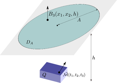
The geometry of the described setting is schematically shown in Figure 1.1. This corresponds, up to a truncation of rectangular magnetic field map, to an experimental set-up of the Paleomagnetism lab at Earth, Atmospheric and Planetary Sciences Department (EAPS), Massachusetts Insitute of Technology, involving a SQUID magnetometer, see [15]. Moreover, with an extra preprocessing step of the field data, this also extends to the QDM magnetometer set-up used in the Paleomagnetism lab at Harvard University [6].
A quantity of basic physical interest is the net magnetisation moment:
| (1.3) |
As discussed above, this is a constant vector equal to the overall magnetisation of the sample which can be determined uniquely (unlike the full magnetisation distribution which essentially enters only in the divergence form, see (1.1) and discussions in [3]). In what follows, we may use slightly different names for this quantity interchangeably: net moment, net magnetisation, zeroth-order algebraic moment of a magnetisation distribution. When is not a regular function but a distribution, the integral in (1.3) should be understood componentwise as the pairing of a compactly supported distribution with the constant function on .
Denote , the (horizontal) disk of radius centered at the origin .
The main result of this work is summarised in the following theorem.
Theorem 1.1.
Assume that (a compactly supported vector distribution) whose support is contained in some bounded set and which produces a magnetic field with vertical component given by (1.2) for . Suppose that the measurement area disk is sufficiently large so that the following condition holds
| (1.4) |
Then, the components of the net moment (1.3) can be asymptotically
estimated, with different orders of accuracy, using the following formulas.
First-order estimates:
| (1.5) |
Second-order estimates:
| (1.6) |
| (1.7) |
Third-order estimates:
| (1.8) |
| (1.9) |
Fourth-order estimates:
| (1.10) |
| (1.11) |
Fifth-order estimates:
| (1.12) |
Remark 1.2.
It is not difficult to see that condition (1.4) can be replaced with
| (1.13) |
Indeed, (1.4) was obtained from
Here, the validity of the left inequality is trivial since
whereas the right inequality can be rewritten as
By the symmetry of the area , we can change the signs in front of and . Recognising the complete square on the left-hand side and dividing over the expression from the right-hand side, we arrive exactly at the fraction appearing in (1.13).
Finally, we note that inequality (1.13) can be ensured by imposing a stricter but geometrically simpler condition
| (1.14) |
where is the orthogonal projection of onto the plane (i.e., the largest horizontal section of ), is the diameter of this set and is the distance between the boundary of the measurement area and .
Remark 1.3.
Here and onwards (except numerics in Section 3), for the sake of simplicity, we have assumed the system of physical units such that the constant of magnetic permeability of vacuum is . In general, the right-hand sides of expression (1.2) should have the factor , and, in Si units, N / A2. Consequently, the right-hand sides of all the formulas (1.5)–(1.12) should, in principle, have the factor .
The most relevant papers to the result of Theorem 1.1 are [1, 2] as well as preliminary works [12, Part 3], [4]. Namely, the current work is an extension of one of the methods introduced in [12, Part 3] and briefly summarised in [4]. There, the second-order asymptotic estimates given by (1.6)–(1.7) have already appeared, but have not been rigorously justified. The case of the leading-order asymptotic estimates (in particular, analogs of (1.5) and (1.7)) and their justification were considered for the case of a rectangular measurement area. The roots of the Fourier analysis of the magnetic field aimed to recover the net moment of a planar magnetisation (i.e. when support set is two-dimensional and parallel to the measurement plane) can already be found in [8, 3, 7]. In [1], the authors considered a more general problem of finding linear net moment estimators (analogs of polynomials appearing in the integrals of (1.5)–(1.12)), without resorting to the asymptotic analysis (hence with no assumption on the largeness of the measurement area), but under restriction that the magnetisation distribution is planar and regular (square-integrable). Ill-posedness of the problem (due to sensitivity of the result to the magnetic field data) was recognised and its regularised version was proposed and dealt with numerically. Finally, in a very recent work [10], the authors adapted high-order multipole expansion to the planar field data for improved recovery of the dipolar coefficients (and hence the net moment) of a volumetric sample. This has generalised the previous work on the dipolar fit methodology [9] which was already efficient for samples with a localised magnetisation distribution.
It should be mentioned that even though recovery of the net moment of a sample, our primary concern, is an important practical problem on its own right, it can also serve, under appropriate assumptions, as a preliminary step for finding a magnetisation distribution. Indeed, while it is unrealistic to retrieve 3 magnetisation components (functions or, more generally, distributions), , , , from the partial knowledge of only one function (see (1.2)), the problem simplifies significantly for a class of samples which are unidirectionally magnetised. Since quantifying the net moment of a sample implies a definite magnetisation direction, it is thus an essential element in this complete reconstruction procedure, see [7].
The structure of the paper is as follows. Section 2 has a twofold goal. First, it is meant to show how one idea based on straightforward Fourier analysis can yield the simplest version of asymptotic net moment estimates for both tangential and normal components. Second, this section illustrates that, by means of a careful asymptotic analysis, the explicit estimates can be not only proved rigorously but also extended to higher orders. Hence, this material exactly constitutes the proof of Theorem 1.1. Then, in Section 3, we illustrate the results numerically on the case where the magnetisation has a singular support (a collection of dipoles is modelled by magnetisation distribution that is a sum of Dirac delta functions) and deal with some practical aspects of the obtained estimates. Finally, we conclude with Section 4 summarising the work, discussing the results and outlining further research directions.
2. Proof of Theorem 1.1
2.1. Some notation and preparatory transformations
Before we proceed with deriving rigorously formulas (1.5)–(1.12) and thus proving Theorem 1.1, let us introduce some useful notations. We shall use the following notational shortcut for the integral of the magnetisation distribution against monomials
| (2.1) |
where we denoted , the set of natural numbers including zero. Following this convention, for the sake of brevity, we may also write, for example,
Note that, when magnetisation is not a function but merely a distribution, the integrals above should be understood as distributional pairing between a compactly supported distribution and smooth monomials on with , , .
Let us denote the two-dimensional Fourier transform which, by our convention, is defined as
where stands for the imaginary unit, and is the Euclidean inner product. With this definition, the differentiation and convolution properties of Fourier transform have the form
| (2.2) |
| (2.3) |
We also note that the Fourier transform of the two-dimensional Poisson kernel is well-known (see e.g. [14, Sect. 4.2]), that is, for any , we have
| (2.4) |
Let us now rewrite (1.2) as
| (2.5) | ||||
Taking Fourier transform of (2.5) in both and variables, we use (2.2), (2.3) and employ (2.4) twice: with in the first line of (2.5), and with in the second one. We thus arrive at
| (2.6) |
where denotes the vertical projection of the set .
We note that even though (1.5)–(1.6), (1.8), (1.10), (1.12) give estimates for tangential net moment components , , we shall restrict ourselves to dealing only with . The situation with is completely analogous.
First, we are going to illustrate our strategy of the derivation of asymptotic estimates of the net magnetisation moment. Here, we shall be only concerned with the low-order formulas of Theorem 1.1 and we shall omit a rigorous justification step. Then, we shall proceed with formal justification and extension of the result to higher orders.
2.2. Illustration of the basic idea of the derivation of the net moment estimates
We are going to focus on deriving (1.5).
We take in expression (2.6) to obtain
| (2.7) |
Since the magnetisation distribution is compactly supported, the Fourier transforms , , are entire functions in , for each , according to the Paley-Wiener theory (see e.g. [13, Thm 4.1]). In particular, power-series expansion of , , about the origin of the complex plane gives
Combining this expansion with the straightforward identities
and the Taylor expansion in of the exponential factor in (2.7)
we obtain
| (2.8) |
| (2.9) |
Here, the remainder term is uniformly small for all due to the boundedness of the set .
On the other hand, we can write
| (2.10) |
We note that in the first term on the right-hand side of (2.10), the integration range is finite and hence an expansion in powers of simply follows from that of the exponential factor:
| (2.11) | ||||
and hence
| (2.12) |
| (2.13) |
Producing an expansion in powers of of the second term in (2.10) is much less straightforward and requires a preliminary simplification. More precisely, we expand the field for large and, assuming largeness of the region , retain only first few terms of this expansion. Namely, from (1.2), we have
| (2.14) |
Consequently, passing to the polar coordinates using , , , we can write
where the residue term is expected to be for sufficiently small values of .
Furthermore, taking real and imaginary parts of both sides, we obtain, respectively,
| (2.15) |
| (2.16) |
where we took into account that
according to the results of Lemma A.4.
Next, as it turns out (see Subsection 2.3 for more details), the integrals on the right-hand sides of (2.15)–(2.16) can be evaluated explicitly in terms of some cylindrical functions. Known representations of these special functions lead to the desired asymptotic expansions in powers of . In particular, for small , we can deduce that
| (2.17) | ||||
| (2.18) | ||||
where the notation also hides the terms of powers of higher than regardless of the presence of the factors such as .
Therefore, by taking the real part of (2.10) and using (2.12), (2.15) and (2.17), we obtain
Comparing this with (2.8) and, in particular, evaluating both expressions at , we arrive at the following identity:
| (2.19) |
where we took into account that .
Similarly, taking the imaginary part of (2.10), we combine (2.13), (2.16) and (2.18) to deduce that
Comparison of this expression with (2.9) and matching the coefficients of the terms yields
| (2.20) |
where we assumed that, for sufficiently small , we have .
While (2.19), (2.20) imply estimates (1.7), (1.5), respectively, the derivation given above was not rigorous and required additional assumptions on the residue term which was reasonably deemed to be sufficiently small for large but was not estimated uniformly in . We shall now proceed with rigorous analysis which will also make it possible to derive higher-order analogs of estimates (1.5), (1.7).
2.3. Rigorous analysis and higher-order asymptotic estimates
Let us start by improving estimate (2.14). To this effect, we use the following elementary Taylor expansions, convergent for ,
to obtain, for , , , , ,
| (2.21) | ||||
| (2.22) | ||||
where , , , are of a sufficiently large magnitude so that
| (2.23) |
Expansions (2.21)–(2.22) imply that, for , (1.2) can be written as
| (2.24) |
with
| (2.25) | ||||
| (2.26) |
| (2.27) |
| (2.28) | ||||
| (2.29) | ||||
| (2.30) |
| (2.31) | ||||
| (2.32) | ||||
| (2.33) | ||||
| (2.34) | ||||
and condition (2.23), for our particular context, rewrites as (1.4).
We are going to pursue the idea outlined in the previous subsection. Namely, comparing a series expansion of (2.7) about with that of (2.10), we shall deduce a set of identities which relate magnetisation moments to the integrals of the measured data on . More precisely, using compactness of the support of the magnetisation , it follows from (2.7) that is a convergent series in powers of whereas is a power series in multiplied by . To facilitate the situation of matching the coefficients of different representations, we shall focus on the region . Consequently, in what follows, evaluation at will mean the limiting value at taken from the positive semiaxis ().
2.3.1. Tangential components of the net moment
Expanding the integrand in (2.7) in power series in a positive neighborhood of and taking the imaginary part, we deduce:
| (2.35) |
| (2.36) | ||||
| (2.37) | ||||
| (2.38) | ||||
| (2.39) | ||||
| (2.40) | ||||
On the other hand, from (2.10), we have, for ,
| (2.41) | ||||
We shall proceed in 3 steps. First, we evaluate the integral
| (2.42) |
and compute its derivatives appearing on the second line of (2.41), hence obtaining a set of valuable identities. Second, we estimate the derivatives of the remainder
| (2.43) |
in order to show that the contribution of the term in the third line of (2.41) is not significant for large (for the chosen order of the asymptotic expansion). Finally, at the last step, we combine the obtained identities and derive asymptotic formulas (1.5)–(1.6), (1.8), (1.10), (1.12) in a rigorously justified fashion.
Step 1: Derivation of the set of identities
Using (2.25) and passing to the polar coordinates using , , , we obtain from (2.42)
| (2.44) |
where
| (2.45) |
| (2.46) |
| (2.47) |
Here, we used results (A.42)–(A.43) of Lemma A.4 multiple times to deduce vanishing of the integrals associated with the terms which involve , , , , , , .
We now employ the integral representation of Bessel functions, given in (A.5), to rewrite, for ,
| (2.48) |
| (2.49) | ||||
| (2.50) | ||||
Note that, in (2.49)–(2.50), we employed integration by parts twice using the asymptotic behavior of given in (A.6).
Using the results of Lemmas A.2–A.3, we have
| (2.51) | ||||
| (2.52) | ||||
| (2.53) | ||||
Therefore, (2.44) together with (2.51)–(2.53) furnishes an explicit form of (2.42). In particular, using (A.2), (A.11), we can compute
| (2.54) |
| (2.55) |
| (2.56) |
| (2.57) |
| (2.58) |
| (2.59) |
Taking into account (2.42), (2.43), we use (2.35)–(2.40) and (2.54)–(2.59) in (2.41) with , respectively, and thus arrive at the following set of identities:
| (2.60) |
| (2.61) |
| (2.62) |
| (2.63) |
| (2.64) |
| (2.65) |
Step 2: Analysis of the remainder terms for
We shall now show that the remainder terms with given by (2.43) (with , as assumed before), can be estimated, for , as follows
| (2.66) |
Proceeding with higher-order terms in the expansions in (2.21)–(2.22), and hence also in (2.24), we notice that we can write, for ,
| (2.67) |
with some constants for , . Consequently, we consider, for ,
| (2.68) | ||||
First of all, we deal with the term on the second line. The integrand is regular and, for , it decays at infinity sufficiently fast so that the differential operator with can be passed under the integral sign. We can thus estimate
for some constant such that
and such a bound is possible due to the remainder estimate in (2.67). Here, in the third line of the estimates, we used the fact that the integral in converges for , , which is true for . For such , the obtained estimate of order is clearly even better than was aimed for (recall (2.66)).
We now fix and proceed with estimating the term in the first line of (2.68). Upon substitution of (2.67) in (2.43) and use of polar coordinates (with , , as before), let us observe that, due to Lemma A.4 (namely, identities (A.42)–(A.43)), the only non-vanishing terms stemming from the part are those proportional to
| (2.69) |
Since we can write
with denoting a binomial coefficient, we deduce that, to estimate , it suffices only to consider the quantities
| (2.70) |
and, in particular, their derivatives evaluated at from the right: , .
Note that the relation between (2.69)–(2.70)
and in (2.67) is , . In other words,
in the asymptotic expansion of the field at infinity, not
every term contributes to , but only the
terms of every second order in , i.e. ,
and so on.
Therefore, we can consider only for ,
where designates the integer part
of .
To sum up, we need to show that, for all , and , we are able to produce an estimate
| (2.71) |
For , we have
and hence
where the convergence of the last integral is due to . The obtained estimate is in agreement with (2.71) since .
To treat the case , a more careful estimate is needed. To this end, it is convenient to make use of the integral representation of the Bessel function given by (A.5) and rewrite (2.70) as
We then evaluate
| (2.72) | ||||
where, in passing the differential operator under the integral sign, we took into account the asymptotic behavior at infinity of given by (A.6) and, on the second line, employed the following identity valid for :
Now, recalling the analytic character of the function (see beginning of Appendix) and, more precisely, its series representation given by (A.2), it is clear that every derivative of of even order is also analytic and vanishes at zero. This implies analyticity of the function and, consequently, a bound on its every derivative at the origin. Therefore, from (2.72), we deduce that
for some constant , and hence (2.71) follows due to the fact that .
Step 3: Asymptotic estimates for the net moment components
Recalling that (according to (2.35)) and using (2.66), we obtain from (2.60)
| (2.73) |
Similarly, using (2.66), we rewrite (2.61)–(2.65), respectively, as
| (2.74) | ||||
| (2.75) | ||||
| (2.76) | ||||
| (2.77) | ||||
| (2.78) | ||||
While the first-order estimate for given in (1.5) follows immediately from rigorously justified (2.73), the higher-order estimates require more work. Namely, we wish to combine (2.74)–(2.78) in order to eliminate in (2.73) the terms with
| (2.79) |
and, at the same time, would not commit a larger error (in order of ) than that of the eliminated term.
Expressing in terms of quantities from (2.74) and inserting it into (2.73), we deduce the second-order estimate for given by (1.6). We note, however, that, for third or higher order estimates, identity (2.74) is not useful due to the fact that its right-hand side has an unknown quantity appearing of order which will block any further effort to increase the accuracy of estimates.
Derivation of the third-order estimate given by (1.8) is analogous to the previous one with the only difference that is expressed (now in terms of quantities) from (2.75) rather than from (2.74).
To proceed with derivation of estimates (1.10) and (1.12), it is convenient first to rewrite (2.75)–(2.78), respectively, as
| (2.80) |
| (2.81) |
| (2.82) |
| (2.83) |
It is easy to see that
| (2.84) |
To obtain the fourth-order estimate for given in (1.10),
we shall use (2.80)–(2.82).
We start by using the first equation of (2.84) (together
with definitions (2.80)–(2.82)) to express
up
to order , namely,
| (2.85) |
Second, we observe that the quantity appearing in (2.73) is related to (2.80)–(2.82) as follows:
| (2.86) | ||||
Finally, substitution of (2.86) in (2.73) followed by the use of (2.85) furnishes (1.10).
2.3.2. Normal component of the net moment
Similarly to the case of tangential net moment components, we expand the integrand in (2.7) in power series in a positive neighborhood of , but, in contrast to that previous situation, the attention will now be on the real part. This yields
| (2.89) |
| (2.90) | ||||
| (2.91) | ||||
| (2.92) | ||||
| (2.93) | ||||
| (2.94) | ||||
On the other hand, (2.10) implies that, for ,
| (2.95) | ||||
As before, we continue in 3 steps. First, we evaluate explicitly
| (2.96) |
that allow us to obtain from (2.95), a set of useful identities involving remainder terms. Second, we estimate the remainder terms, namely,
| (2.97) |
for large . At last, we rigorously derive asymptotic formulas (1.7), (1.9), (1.11) from the obtained set of identities.
Step 1: Derivation of the set of identities
Using (2.25) and passing to the polar coordinates using , , , we obtain from (2.96)
| (2.98) |
where
| (2.99) |
| (2.100) |
| (2.101) |
Here, we used results (A.40)–(A.41) of Lemma A.4 multiple times to deduce vanishing of the integrals associated with the terms which involve , , , , , , .
Using the integral representation of Bessel functions (due to (A.4)), integration by parts, the asymptotics of given by (A.6), and the relation (see (A.10)), we can write, for ,
| (2.102) | ||||
| (2.103) | ||||
| (2.104) | ||||
Inserting here the results of Lemmas A.2–A.3, namely, (A.22), (A.34)–(A.35), we arrive at
| (2.105) | ||||
| (2.106) | ||||
| (2.107) | ||||
Substitution of (2.105)–(2.107) into (2.98), we employ (A.2) and (A.11) to compute
| (2.108) |
| (2.109) |
| (2.110) |
| (2.111) |
| (2.112) |
| (2.113) |
Taking into account (2.96), (2.97), we use (2.89)–(2.94) and (2.108)–(2.113) in (2.95) with , respectively, and thus arrive at the following set of identities:
| (2.114) |
| (2.115) |
| (2.116) |
| (2.117) |
| (2.118) |
| (2.119) |
Step 2: Analysis of the remainder terms for
We shall show that
| (2.120) |
The reasoning will we identical to that of Step 2 of Subsection 2.3.1, therefore, we omit repetition of some details.
Using previously introduced notation (see (2.67)), we can write
| (2.121) | ||||
We now fix and proceed with estimating the term on the first line of (2.120). Identities (A.40)–(A.41) of Lemma A.4 entail that the only non-vanishing terms are those of the form
| (2.122) |
and hence it is sufficient to only deal with the quantities
| (2.123) |
As before, in (2.122)–(2.123) is related to from (2.67) as , : only the terms , , …, in (2.67) contribute to . Hence, we consider only for .
We are intending to show that the following estimate holds for all , , :
| (2.124) |
For , we have
and hence
where the convergence of the last integral is due to . The obtained estimate satisfies (2.124) due to .
For , we use (A.4) to rewrite (2.123) as
We then evaluate
| (2.125) | ||||
where the following identity, for , was used:
Due to analyticity (see beginning of Appendix), we see from (A.2) that its every derivative of odd order is also analytic and vanishes at zero. Hence, is analytic as well, and, in particular, has bounded derivatives at the origin. Therefore, (2.125) entails that
for some constant , and hence (2.124) follows due to the fact that .
Step 3: Asymptotic estimates for the net moment component
Since, according to (2.26), we have , and hence using (2.120), it follows from (2.114) that
| (2.126) |
Employing (2.66), we rewrite (2.61)–(2.65), respectively, as
| (2.127) | ||||
| (2.128) | ||||
| (2.129) | ||||
| (2.130) | ||||
| (2.131) | ||||
We see that (2.126) already provides the second-order estimate of given in (1.7). The higher-order estimates given by (1.9) and (1.11) can be obtained by combining (2.128)–(2.130). Note that elimination of using either (2.127) would incur a rather large error , reducing the final estimate to the first order. Similarly, any use of (2.131) would result in an estimate of order , but such an estimate could already be deduced using the other listed above relations.
For the sake of simplification, let us set
| (2.132) |
and rewrite (2.126) and (2.128)–(2.130), respectively, as
| (2.133) |
| (2.134) |
| (2.135) |
| (2.136) |
| (2.137) |
There are multiple ways to combine equations (2.133)–(2.137) to eliminate and . In particular, we should use the following two relations which are straightforward to verify:
| (2.138) |
3. Numerical validation and practical considerations
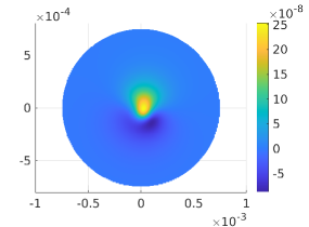
We demonstrate results by performing a numerical simulation on a synthetic example. In this example, we choose magnetisation distribution to consist of 4 magnetic dipoles: with denoting Dirac delta function. The positions and the components of dipolar moments of each dipole are given in Table 1.
| m | m | m | m | |
| m | m | m | m | |
| m | m | m | m | |
The net moment of this magnetisation distribution is equal to
| (3.1) |
The produced magnetic field is given by
| (3.2) |
and is measured on the disk at the height m. Since we now work in Si units, we should recall Remark 1.3 and take into account the previously omitted factor N / A2.
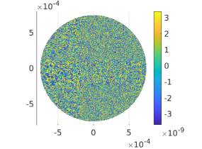
In order to check robustness of the moment estimates obtained in Theorem 1.1, we also perform simulations on data with a synthetic noise. Namely, we modify using additive Gaussian white noise with the amplitude , where SNR is the signal-to-noise ratio (in decibels) and is the variance of on . For our simulations, we choose dB which corresponds to the noise level.
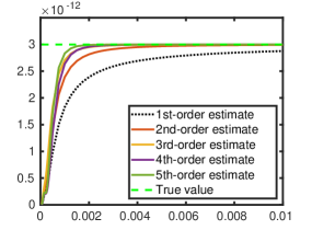
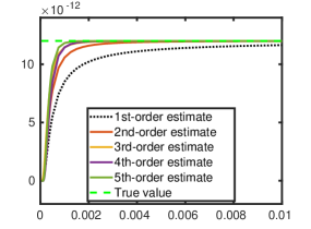
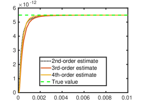
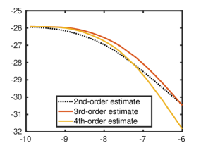
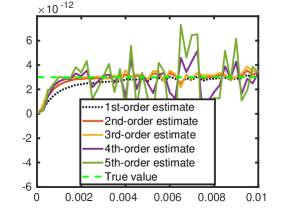
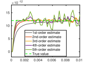
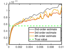
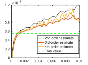
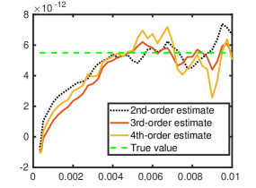
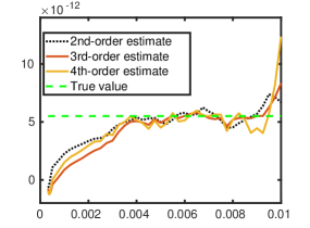
We shall now compute the integrals on the right-hand sides of (1.5)–(1.12) for different values of . According to our asymptotic result for large , we expect to see that, as grows, the values of each of these integrals converge, with a different rate, to the value of a component of the net moment given by (3.1). Figures 3.2–3.3 show exactly that for the tangential and normal net moment components, respectively. We note that in Figure 3.3 and further figures involving the normal net moment component , a pair of the estimates are used: one with in (1.9), (1.11) and the other with .
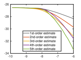
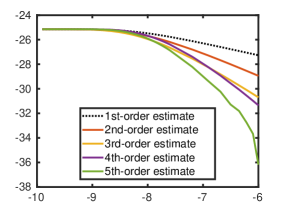
To illustrate the different convergence rates better, in Figures 3.4–3.5, we plot the differences , , against . This, in general, shows agreement with the estimates of the remainder term given in (1.5)–(1.12).
Finally, in Figure 3.6, we directly test the estimates of the net moment components when the magnetic field is contaminated by noise (with the noise model discussed above). We observe the persistence of the estimates for the tangential net moment components , , even though higher-order estimates perform worse. The situation is different for the estimates for the normal component in that the estimates of any order clearly have a growing trend with the increase of , see Figure 3.7. This is deemed to be due to the presence of the factor in all estimates (1.7), (1.9), (1.11) resulting in the noise amplification for large . The issue, however, can be dealt with. One of possible remedies is demonstrated in Figure 3.8. There, a simple -point linear backward regression was used: namely, for each fixed value , (nearest) points with smaller values of (hence lying within the same original measurement disk ) were used to establish and subtract a linear trend in .
Let us now briefly comment on the fact that we chose to illustrate the results on a magnetisation distribution with a singular support. Besides its simplicity, this choice is physically motivated as any magnetisation can be thought of a combination of dipole sources. From mathematical (numerical) viewpoint, a magnetic field produced by continuous magnetisation distribution is given by the integral whose numerical approximation (quadrature rule) is nothing but a weighted sum of dipoles. Consequently, we do not expect results for continuous magnetisation distributions to be of any drastical difference. On the other hand, this highlights the applicability of our methodology to the magnetisations that could be much more singular than smooth or square-integrable functions.


4. Discussion and conclusion
Motivated by a concrete experimental set-up, we considered a problem of estimating net magnetisation of a sample from one component of the magnetic field available in the limited measurement area in the plane above the sample. We approached this problem asymptotically, assuming the size of the measurement area to be large. We derived a set of explicit formulas for the asymptotic estimates of all three components of the net moment. For simplicity, we considered only the case of the circular geometry, i.e. where the measurement area is a disk. Analogous results to those in Theorem 1.1 could be deduced by our method also for the rectangular geometry which technically is even closer to what is used in Paleomagnetism lab at EAPS department of MIT, USA. The main difference in obtaining such results with the present approach would be a technique of the asymptotic estimation of Fourier integrals (such as the second term in the right-hand side of (2.10)) which involve both a large and a small parameter (and hence must likely rely on a partial availability of explicit integration formulas).
In this paper, we have obtained and proved asymptotic estimates up to order for the tangential net moment components , and up to order for the normal component . The main purpose was, however, to introduce a machinery that can generate asymptotic estimates of an arbitrary order. It is clear from the proof of Theorem 1.1 and auxiliary computations in Appendix that the asymptotic order of the estimates can be upgraded by proceeding in an established manner. This would require integration of the field against polynomials of a higher order. Practical advantages of it, however, are not yet obvious. First, such estimates are expected to be sensitive to any noise in : it was demonstrated in Section 3 that while lower- and middle-order estimates lead to expected results, estimates of higher orders are much more prone to the noise. Second, when pursuing an estimate of a higher order, one should not forget that the obtained result is of only asymptotic nature: while a high-order estimate would be advantageous for very large values of , it may not be so for a smaller due to a potentially large value of a multiplicative constant (in ) in the remainder term. In particular, while Figure 3.2 shows a significant improvement due to the use of the second-order estimates compared to those of the first-order, the same figure together with Figure 3.3 demonstrate that, even without any noise, a higher-order estimate may be suboptimal for mid-range values of . A relevant issue to bear in mind is that, apart from the basic asymptoticness condition given by (1.4) (see also (1.14)), proceeding to higher-order estimates assumes implicitly (but it is evident from the form of the remainder terms) that the magnetisation is sufficiently localised so that its higher algebraic moments , , (see (2.1)) do not grow too fast with respect to their order , namely, that the quantities are not large for the value of in question. A conclusion to draw from these observations is that the middle-order estimates (e.g. those of orders -) are perhaps the best: both from practical prospective of proximity to the true value of the net moment and from the viewpoint of the robustness to imperfect measurements. One can also consider a possibility of choosing an estimate which is best possible for a given magnitude of . This is pertinent to the problem of finding an optimal truncation of asymptotic series.
In future works, we should study relation of our asymptotic results to the stable estimates of the net moment using constrained optimisation approach, in particular those obtained in [1] for the planar and regular (square-integrable) magnetisation. The strength of that approach is in its generality (potentially giving more than just a net moment estimate) and, in particular, that the result does not require any largeness of the measurement area size. However, it does not furnish explicit formulas for the net moment estimates: the obtained estimators (i.e. functions that the field needs to be integrated against in order to estimate a net moment component; in our case these are polynomials) could only be computed numerically by solving an integral-partial-differential equation. Moreover, these estimators, despite being a solution of a regularised version of the problem, could be seen to have rather irregular behavior with a rapid growth near the end of the measurement area and, as the authors noted, this feature is not the most practical factor of their result. Studying other ways of stabilisation of the estimates and regularisation is also important. In this respect, it is natural to ask a question: what is the best way of using redundancy of a set of the asymptotic formulas for the net moment components to arrive at an estimate with the minimal effect of noise or to have the fastest (non-asymptotic) convergence to the true value of a net moment? For example, in the present approach, we have a natural redundancy for all estimates of of order and higher due to the freedom of choice and in formulas (1.9), (1.11) and so on. In Figure 3.3, these estimates give almost indistinguishable results (it can be checked that the difference between the two is not zero but very small), and hence may not look directly useful. However, since having more relations than unknown quantities is always better when dealing with noise, this is still an advantage. Also, it is clear from Step 3 of the proof of Theorem 1.1 that, upon involving higher order polynomials, a richer set of lower-order estimates could be obtained.
Another path for a possible future work is to explore the possibility of obtaining asymptotic expansions analogous to those given in Theorem 1.1 but relying on the smallness of a slghtly different asymptotic parameter. Namely, if, instead of and in (2.21) and (2.22), respectively, one factored out and and proceeded with appropriate modifications, the final asymptotic results would have a larger area of validity than that described by (1.4). In particular, this would cover a reduction to a dipolar case when the measurement area is not necessarily large but the constant is. Since in the mentioned experimental set-up, the height is small, this modification would yield a little practical benefit but would complicate analysis of Fourier integrals.
Finally, the results of this work naturally connect to the issue of the asymptotic field extension. Indeed, the asymptotic field expansion at infinity (2.24) is seen to feature at the leading order and quantities , at the next order. While the estimates of are given, to a different order, in (1.7), (1.9) and (1.11), it is evident from the proof of Theorem 1.1, that the quantities , can also be asymptotically estimated, see e.g. (2.85) and (2.87) (and their versions with replaced by , as well as their lower-order analogs). Thus, this furnishes an explicit -term expansion of at infinity which, in general, when solving inverse magnetisation problems, should serve as a better alternative to a simple prolongation of the field by zero outside of the measurement area. Such a strategy can also potentially be used in setting up an iterative scheme. Of course, all of this is meaningful only when the actual measurement area is already sufficiently large so that the asymptotic estimates for , , are sufficiently accurate.
Acknowledgements
The author acknowledges inspiring discussions on the topic of inverse magnetisation problems with L. Baratchart, S. Chevillard, J. Leblond, C. Villalobos-Guillen (Centre Inria d’Université Côte d’Azur, France), D. Hardin (Vanderbilt University, USA) and E. A. Lima (MIT, USA).
Appendix A
We collect here several useful results about cylindrical functions and some relevant integrals. In what follows we will use the notation to denote natural numbers, , and the notation for integer numbers.
Basic facts about Bessel, Neumann and Struve functions
The Bessel function of order is an entire function satisfying the differential equation [11, (10.2.1)]
| (A.1) |
We have the following series expansion [11, (10.2.2)]
| (A.2) |
which, due to the entire character of , is absolutely convergent
for every . Here, denotes the Euler gamma
function, for which we have, in particular,
for . Moreover, it is worth noting that
for , which implies vanishing
of negative powers of in expansion (A.2) even
for negative orders .
The following integral representation holds [11, (10.9.1)]
| (A.3) |
In particular,
| (A.4) |
| (A.5) |
For , , the leading order asymptotics reads [11, (10.17.2)]
| (A.6) |
where the estimate of the remainder term is due to the discussion
in [11, Sect. 10.17(iii)].
The Bessel functions , satisfy the connection
formula [11, (10.4.1)]
| (A.7) |
as well as simple recurrence relations [11, (10.6.1)]
| (A.8) |
| (A.9) |
In particular, (A.7) and (A.9) entail that
| (A.10) |
The Struve function of order is an entire function defined by the absolutely convergent power series [11, (11.2.1)]
| (A.11) |
The companion Struve function of order is defined [11, (11.2.5)] as
| (A.12) |
where is the Neumann function.
For , , the following asymptotics hold
true [11, (11.6.1)]
| (A.13) |
| (A.14) |
and the remainder terms are discussed in [11, Sect. 11.6(i)] and [11, Sect. 10.17(iii)], respectively. The asymptotic behavior of for , , hence follows from (A.12)–(A.14). In particular, for ,
| (A.15) |
| (A.16) |
Moreover, we have the following connection formula
| (A.17) |
Some useful integrals pertinent to the cylindrical functions
The following lemmas establish several integral relations which are also crucial for the proof in Section 2.
Lemma A.1.
For , , the following identity holds
| (A.18) |
Proof.
First, upon integration by parts (using the asymptotic behavior at infinity of given by (A.6)), we have
| (A.19) |
Then, if we employ (A.1) to express in terms of and , we obtain
and hence
| (A.20) |
On the other hand, returning to (A.19) and integrating it by parts again, we arrive at
| (A.21) | ||||
Here, in the second line, we eliminated the intergral term involving using (A.20).
Lemma A.2.
For , we have
| (A.22) |
Proof.
Note that using (A.8), we have
| (A.23) |
Let us start by transforming the first term in (A.23), namely,
| (A.24) | ||||
Here, in the first line, we employed integration by parts (together with the asymptotic behavior at infinity of given by (A.6)). To arrive at the second line, we used the identity
implied by (A.1).
Expressions (A.24) and (A.25) imply that the integral on the left-hand side of (A.23) is expressible in terms of two integral quantities: and . Let us now show that these quantities are simply related:
| (A.26) |
and, moreover,
| (A.27) |
Recalling asymptotics (A.6), we note that the integrals on the left-hand sides of (A.26), (A.27) are not absolutely convergent, and hence an additional care with technical manipulations is needed. Namely, we shall first replace the integration range with for arbitrary finite , and then pass to the limit as . We shall proceed in several steps.
Step 1: Establishing (A.26)
We start with (A.26) and use integral representation (A.3):
Consequently, exchanging the order of integration (permissible due to the regularity of the integrand and finiteness of the integration limits), we obtain
| (A.28) | ||||
where we used the identities
and, except for the last one, also their analogs with instead
of . The first two of these identities are purely trigonometrical
whereas the last two are due to (A.4)–(A.5).
Passing to the limit in (A.28)
using asymptotics (A.6), we thus conclude with
(A.26).
Step 2: Establishing (A.27)
To deduce relation (A.27), we use [11, (10.22.2)] to write
| (A.29) | ||||
where we used (A.7), (A.17) in passing
to the second line.
Note that, employing asymptotics (A.6), (A.15)–(A.16),
we have, for ,
Therefore, by passing to the limit as in (A.29), we obtain (A.27).
Step 3: Conclusion of the proof
Lemma A.3.
Proof.
Application of Lemma A.1 with yields
| (A.38) |
Lemma A.4.
For , , , we have the following identities
| (A.40) |
| (A.41) |
| (A.42) |
| (A.43) |
Proof.
Using periodicity of the integrand, we can shift the interval from to and further split it in two:
| (A.44) | ||||
Performing the change of variable , in each of the integrals on the second line of (A.44), we have
Here, we used the fact that for and for which makes both integral quantities on the second line of (A.44) opposite to each other in sign and thus entails (A.40).
To show (A.41), a useful change of variable is , . This, upon splitting the integration range to into and , leads to
Finally, to show (A.43), we use the fact that identity (A.40) holds, in particular, for any with arbitrary . Integrating it in over this interval and interchanging the order of integration (permissible by the regularity of the integrand and the finite integration range), we obtain
Since the same reasoning also works by working with an interval , identity (A.43) is thus proved up to a change of the notation to . ∎
References
- [1] Baratchart, L., Chevillard, S., Hardin, D., Leblond, J., Lima, E., Marmorat, J. P., “Magnetic moment estimation and bounded extremal problems”, Inverse Problems and Imaging, 13 (1), 2019.
- [2] Baratchart, L., Chevillard, S., Leblond, J., Lima, E., Ponomarev, D., “Asymptotic method for estimating magnetic moments from field measurements on a planar grid” (preprint), HAL Id: hal-01421157, 2018.
- [3] Baratchart, L., Hardin, D. P., Lima, E. A., Saff, E. B., Weiss, B. P., “Characterizing kernels of operators related to thin-plate magnetizations via generalizations of Hodge decompositions”, Inverse Problems, 29 (1), 2013.
- [4] Baratchart, L., Leblond, J., Lima, E., Ponomarev, D., "Magnetization moment recovery using Kelvin transformation and Fourier analysis", J. Phys. Conf. Ser., 904, 2017.
- [5] Baratchart, L., Villalobos-Guillen, C., Hardin, D. P., Northington, M. C., Saff, E. B., “Inverse potential problems for divergence of measures with total variation regularization”, Foundations of Computational Mathematics, 20 (5), 1273–1307, 2020.
- [6] Fu, R. R., Lima, E. A., Volk, M. W., Trubko, R., “High-sensitivity moment magnetometry with the quantum diamond microscope”, Geochemistry, Geophysics, Geosystems, 21 (8), 2020.
- [7] Lima, E. A., Weiss, B. P., Baratchart, L., Hardin, D. P., Saff, E. B., “Fast inversion of magnetic field maps of unidirectional planar geological magnetization”, J. Geophys. Res.: Solid Earth, 118 (6), 2723–2752, 2013.
- [8] Lima, E. A., Weiss, B. P., “Obtaining vector magnetic field maps from single-component measurements of geological samples”, Journal of Geophysical Research: Solid Earth, 114 (B6), 2009.
- [9] Lima, E. A., Weiss, B. P., “Ultra-high sensitivity moment magnetometry of geological samples using magnetic microscopy”, Geochemistry, Geophysics, Geosystems, 17 (9), 3754–3774, 2016.
- [10] Lima, E. A., Weiss, B. P., Borlina, C. S., Baratchart, L., Hardin, D. P., “Estimating the net magnetic moment of geological samples from planar field maps using multipoles”, Geochemistry, Geophysics, Geosystems, 24, 2023.
- [11] Olver, F. W. J., Lozier, D. W., Boisvert, R. F., Clark, C. W., “NIST Handbook of Mathematical Functions”, Cambridge University Press, 2010.
- [12] Ponomarev, D., “Some inverse problems with partial data”, Doctoral thesis, Université de Nice - Sophia Antipolis (University of Côte d’Azur), 2016.
- [13] Stein, E. M., Weiss, G., “Introduction to Fourier Analysis on Euclidean Spaces”, Princeton University Press, 2016.
- [14] Strichartz, R., “Guide to Distribution Theory and Fourier Transforms”, CRC Press, 1994.
- [15] Weiss, B. P., Lima, E. A., Fong, L. E., Baudenbacher, F. J., “Paleomagnetic analysis using SQUID microscopy”, Journal of Geophysical Research: Solid Earth, 112 (B9), 2007.