Unfooling Perturbation-Based Post Hoc Explainers

Abstract

Monumental advancements in artificial intelligence (AI) have lured the interest of doctors, lenders, judges, and other professionals. While these high-stakes decision-makers are optimistic about the technology, those familiar with AI systems are wary about the lack of transparency of its decision-making processes. Perturbation-based post hoc explainers offer a model agnostic means of interpreting these systems while only requiring query-level access. However, recent work demonstrates that these explainers can be fooled adversarially. This discovery has adverse implications for auditors, regulators, and other sentinels. With this in mind, several natural questions arise – how can we audit these black box systems? And how can we ascertain that the auditee is complying with the audit in good faith? In this work, we rigorously formalize this problem and devise a defense against adversarial attacks on perturbation-based explainers. We propose algorithms for the detection (CAD-Detect) and defense (CAD-Defend) of these attacks, which are aided by our novel conditional anomaly detection approach, KNN-CAD. We demonstrate that our approach successfully detects whether a black box system adversarially conceals its decision-making process and mitigates the adversarial attack on real-world data for the prevalent explainers, LIME and SHAP.

1 Introduction

As a result of the many recent advancements in artificial intelligence (AI), a significant interest in the technology has developed from high-stakes decision-makers in industries such as medicine, finance, and the legal system (Lipton 2018; Miller and Brown 2018; Rudin 2019). However, many modern AI systems are black boxes, obscuring undesirable biases and hiding their deficiencies (Szegedy et al. 2014; Hendrycks et al. 2021; Lipton 2018). This has resulted in unexpected consequences when these systems are deployed in the real world (O’Neil 2016; Buolamwini and Gebru 2018; McGregor 2021). Accordingly, regulatory and legal ordinance has been proposed and implemented (EU and Parliament 2016; U.S.-EU TTC 2022; European Commission 2021).

All of this naturally leads to the question: how can we audit opaque algorithms? Post hoc explanation methods offer a way of understanding black box decision-making processes by estimating the influence of each variable on the decision value. Unfortunately, there is a medley of incentives that may motivate an organization to withhold this information, whether it is financial, political, personal, or otherwise. Indeed, these explainers are demonstrably deceivable (Slack et al. 2020; Baniecki 2022) — if an organization is aware that its algorithms are under scrutiny, it is capable of falsifying how its algorithms operate. This begs the question — how do we know that the auditee is complying faithfully?

In this work, we explore the problem of employing perturbation-based post hoc explainers to audit black box algorithms. To the best of our knowledge, this is the first paper to address the aforementioned questions and provide a solution. We explore a multi-faceted problem setting in which the auditor needs to ascertain that the algorithms of an organization: 1) do not violate regulations or laws in their decision-making processes and 2) do not adversarially mask said processes. Our contributions are as follows:

• We formalize real-world adversarial attack and defense models for the auditing of black box algorithms with perturbation-based post hoc explainers. We then formalize the general defense problem against adversarial attacks on explainers, as well as against the pragmatic scaffolding-based adversarial attack on explainers (Slack et al. 2020).

• We propose a novel unsupervised conditional anomaly detection algorithm based on k-nearest neighbors: KNN-CAD.

• We propose adversarial detection and defense algorithms for perturbation-based explainers based on any conditional anomaly detector: CAD-Detect and CAD-Defend, respectively.

• Our approach is evaluated on several high-stakes real-world data sets for the popular perturbation-based explainers, LIME (Ribeiro, Singh, and Guestrin 2016) and SHAP (Lundberg and Lee 2017). We demonstrate that the detection and defense approaches using KNN-CAD are capable of detecting whether black box models are adversarially concealing the features used in their decision-making processes. Furthermore, we show that our method exposes the features that the adversaries attempted to mask, mitigating the scaffolding-based attack.

• We introduce several new metrics to evaluate the fidelity of attacks and defenses with respect to explanations and the black box model.

• We conduct analyses of the explanation fidelity, hyperparameters, and sample-efficiency of our approach.

2 Background

Local Black Box Post Hoc Explainers

Of particular relevance to auditing an algorithm is in understanding individual decisions. Explainable AI (XAI) approaches afford transparency of otherwise uninterpretable algorithms (Barredo Arrieta et al. 2020) and are conducive to auditing (Akpinar et al. 2022; Zhang, Cho, and Vasarhelyi 2022). Local post hoc explainers, notably LIME and SHAP, do so by estimating the contribution of each feature to a decision value. These particular explainers are classified as model agnostic and black box, which satisfies the conditions of an audit — the auditor has no a priori knowledge of the model class and has only query-level access. Both approaches produce explanations by fitting linear models to a dataset generated by perturbing the neighborhood about a sample. Let $\bm{\mathcal{D}}=(\bm{\mathcal{X}}\times\bm{\mathcal{Y}})=\{(\mathbf{x}_{1},{y}_{1}),(\mathbf{x}_{2},{y}_{2}),\dots,(\mathbf{x}_{N},{y}_{N})\}$ be the data set where each data sample $\mathbf{x}_{i}\in\mathbb{R}^{F}$ has $F$ features and each label ${y}_{i}\in\mathbb{N}_{0}$ represents one of $C$ classes encoded as an integer in the range $[0..C)$. We denote the black box classifier as $f:\bm{\mathcal{X}}\rightarrow\bm{\mathcal{Y}}$ and the explainer as $g$. The general problem these explainers solve in order to explain an instance $\mathbf{x}_{i}$ is given by Eq. (1)

$$\operatorname*{argmin}_{g_{\mathbf{x}_{i}}\in\mathcal{G}}\sum_{\mathbf{x}^{(g)}_{j}\in\bm{\mathcal{X}}_{i}^{(g)}}\left(f(\mathbf{x}^{(g)}_{j})-g_{\mathbf{x}_{i}}(\mathbf{x}^{(g)}_{j})\right)^{2}\pi_{\mathbf{x}_{i}}(\mathbf{x}^{(g)}_{j})\,+\,\Omega(g_{\mathbf{x}_{i}})$$ (1)

The minimization objective is a function of the linear model $g_{\mathbf{x}_{i}}$ from the set of all linear models $\mathcal{G}$, the neighborhood function $\pi_{\mathbf{x}_{i}}$, and the regularization function $\Omega$. With a slight abuse of notation, $\pi_{\mathbf{x}_{i}}$ both generates the neighborhood of $\mathbf{x}_{i}$ ($\bm{\mathcal{X}}_{i}^{\text{(}g\text{)}{}}$) and gives the proximity of each $\mathbf{x}^{\text{(}g\text{)}{}}_{j}$ to $\mathbf{x}_{i}$. The latter two functions are defined using game-theoretic means for SHAP and empirical means for LIME. Both explainers produce explanations as a set of feature contributions $\mathcal{E}_{i}=\{a_{ij}\}_{j=1}^{F}$ that describes the contribution, or importance, of each feature to the decision value $y_{i}$. In our notation, $a_{ij}$ indicates the explained contribution of the $j^{\text{th}}$ feature to $y_{i}$.

Adversarial Attacks on Explainers

Szegedy et al. were the first to discover the phenomena of adversarial examples (Szegedy et al. 2014) — human-indistinguishable manipulation of the input space that results in misclassification. It is worth noting that naturally-occurring adversarial examples have been shown to exist (Hendrycks et al. 2021), though the focus of this work concerns human adversaries. In contrast to the literature on neural network adversarial attacks (Ren et al. 2020), attacks on explainers are comparatively less explored, especially those that are perturbation-based (Baniecki 2022). Slack et al. were the first to propose an adversarial attack on black box post hoc explainers (Slack et al. 2020). The motivation for the attack arose from the observation that explainer perturbations are often off of the data manifold. In the attack, the adversary aims to detect whether some $\mathbf{x}_{i}$ originates from $\bm{\mathcal{X}}$ or from the explainer-generated samples, $\bm{\mathcal{X}}^{\text{(}g\text{)}{}}$, using a scaffolding classifier. $\bm{\mathcal{X}}^{\text{(}g\text{)}{}}$ is generated by perturbing each $\mathbf{x}_{i}\in\bm{\mathcal{X}}$, creating a set of new instances $\bm{\mathcal{X}}_{i}^{\text{(}g\text{)}{}}$. The union of each $\bm{\mathcal{X}}_{i}^{\text{(}g\text{)}{}}$ yields the complete set, i.e., $\bm{\mathcal{X}}^{\text{(}g\text{)}{}}=\bigcup_{i}\bm{\mathcal{X}}^{\text{(}g\text{)}{}}_{i}$. If the adversary determines that the query originates from an explainer, then it can elect to predict using an unbiased model. In effect, the adversary lies to the explainer about how it uses the features. Formally, given a biased predictor $f_{\text{biased}}$ and an unbiased predictor $f_{\text{unbiased}}$, the adversary can toggle between predictors using an out-of-distribution (ood) detector $d{}$ according to Eq. (2).

$$f(\mathbf{x}_{i})=\begin{cases}f_{\text{biased}}(\mathbf{x}_{i})&\text{if }d{}(\mathbf{x}_{i})=1\\ f_{\text{unbiased}}(\mathbf{x}_{i})&\text{otherwise}\end{cases}$$ (2)

The detector $d{}$ is trained on the samples $\bm{\mathcal{X}}\cup\bm{\mathcal{X}}^{\text{(}g\text{)}{}}$ with a corresponding label of ‘0’ if the sample is ood (from $\bm{\mathcal{X}}^{\text{(}g\text{)}{}}$) and ‘1’ otherwise (from $\bm{\mathcal{X}}$). Put simply, the detector $d{}$ determines if the input sample originated from real data or is an explainer-generated perturbation. If the sample origin is predicted to be an explainer, the unbiased predictor $f_{\text{unbiased}}$ makes predictions in an innocuous manner, e.g., independent of sensitive features such as race. The authors demonstrate that the attack obscures the biased use of features, such as making predictions based on race, from LIME and SHAP while maintaining near-perfect prediction fidelity on in-distribution samples.

In related but tangential works, attacks have been developed on the model and explainer simultaneously. Abdukhamidov et al. introduce a gradient-free black box attack on XAI systems that manipulates model predictions without significantly altering the explanations by post hoc explainers (Abdukhamidov et al. 2022). Closely related, Zhan et al. develop a joint attack with the same implications (Zhan et al. 2022). Both works consider explainers that require gradient-level access to the model and are unsuitable for auditing. Noppel et al. propose a trigger-based neural backdoor attack on XAI systems that simultaneously manipulates the prediction and explanation of gradient-based explainers (Noppel, Peter, and Wressnegger 2022). Again, the attack scenario in our work deviates from this model.

Adversarial Defense for Explainers

In a similar fashion, defense against adversarial attacks is well explored in the literature (Ren et al. 2020). However, there is relatively scarce work in defending against adversarial attacks on explainers. Ghalebikesabi et al. address the problems with the locality of generated samples by perturbation-based post hoc explainers (Ghalebikesabi et al. 2021a). They propose two variants of SHAP, the most relevant being Neighborhood SHAP which considers local reference populations to improve on-manifold sampling. Their approach is able to mitigate the scaffolding attack (Slack et al. 2020). While this is a notable achievement, it is unclear how the approach compares to baseline SHAP with respect to quantitative and qualitative measures of explanation quality, whether it still upholds the properties of SHAP explanations, and other concerns (Ghalebikesabi et al. 2021b). Also related is a constraint-driven variant of LIME, CLIME (Shrotri et al. 2022). CLIME has been demonstrated to mitigate the scaffolding attack, but requires hand-crafted constraints based on domain expert knowledge and for data to be discrete.

A step forward in explainer defense, Schneider et al. propose two approaches to detect manipulated Grad-CAM explanations (Schneider, Meske, and Vlachos 2022). The first is a supervised approach that determines if there is (in)consistency between the explanations of an ensemble of models and explanations that are labeled as manipulated or not. The second is an unsupervised approach that determines if the explanations of $f$ are as sufficient to reproduce its predictions as those from an ensemble of models. They conclude that detection without domain knowledge is difficult. Aside from the deviant attack model in their work, we do not require that deceptive explanations be labeled (an expensive and error-prone process) and we require that only a single model be learned (the authors use 35 CNNs as the ensemble in experiments).

Recently, a perturbation-based explainer coined EMaP was introduced that also helps to mitigate the scaffolding attack (Vu, Mai, and Thai 2022). Similar to Neighborhood SHAP, it improves upon its perturbation strategy to create more in-distribution samples. This is accomplished by perturbing along orthogonal directions of the input manifold, which is demonstrated to maintain the data topology more faithfully.

Conditional Anomaly Detection

Vanilla anomaly detection aims to discover observations that deviate from a notion of normality, typically in an unsupervised paradigm (Ruff et al. 2021). Of interest in this work is conditional, also referred to as contextual, anomaly detection. This type of anomaly is an observation that is abnormal in a particular context, e.g., in time or space. Formally, a set of conditional anomalies $\mathcal{A}$ is given by Eq. (3)

$$\mathcal{A}=\{(\mathbf{x}_{i},\mathbf{y}_{i})\in(\bm{\mathcal{X}}\times\bm{\mathcal{Y}})\mid\mathbb{P}(\mathbf{y}_{i}\mid\mathbf{x}_{i})\leq\tau\},~{}\tau\geq 0$$ (3)

where $\mathbb{P}$ is the probability measure of some probability density function (pdf) that characterizes normality and $\tau$ is a low-probability threshold separating normal and abnormal observations. Following the terminology in (Song et al. 2007), $\bm{\mathcal{X}}$ is the set of environmental variables that the set of observed variables $\bm{\mathcal{Y}}$ is conditioned on.

Song et al. proposed the first conditional anomaly detector using Gaussian mixture models — two sets of Gaussians model the environmental and observed variables, respectively, while a learned probability mapping function determines how the Gaussians in each set map to one another (Song et al. 2007). Since, several approaches have been proposed based on classical and deep learning techniques — we point to this comprehensive survey for further reading (Ruff et al. 2021). In this work, we propose a new conditional anomaly detection method as 1) the deep learning techniques are data-hungry and 2) most techniques do not consider or fair well with categorical data, which is plentiful in real-world high-stakes data: credit scoring (FICO 2018), recidivism risk scoring (Angwin et al. 2016), etc.

3 The Problem and a Solution

Figure 1: An overview of the adversarial attack and defense scenario. The top panel mirrors the bottom panel formalism on a higher level. Our defense approach provides defense to auditors from potential adversarial behavior of the auditee, ACME. Given the explainer $g$-generated samples $\bm{\mathcal{X}}^{\text{(}g\text{)}{}}$ and reference samples $\bm{\mathcal{X}}$, the defense $h$ queries the black box $f$. With the results, $h$ gives the auditor the defended explanations $\mathcal{E}$ and a measure of adversarial behavior $D(\cdot,\cdot)$.

The Attack and Defense Models

In the attack scenario, an organization algorithmically makes decisions on behalf of users (customers, patients, employees, etc.) using a black box predictor $f$. Note that $f$ can be a black box due to it being either uninterpretable or proprietary (or both) (Rudin 2019). We will refer to the organization as the ACME (Corporation) for the remainder of the paper. We recommend referring back to Figure 1 as a guide on how elements of the scenario relate. The attacker only provides query-level access to $f$, e.g., via an API, a web form, or even a social media app facial filter. In the case of $f$ being a classifier, only the final decision value is available, not the class-wise probabilities. Moreover, the class of model that $f$ belongs to is assumed to be unknown. Thus, to ensure that ACME meets legal or regulatory compliance, an auditor uses a local post hoc explainer, $g$, to determine how features are used to make individual decisions. Due to a variety of incentives (financial, political, personal, etc.), an adversary within ACME desires to conceal the behavior of $f$. The adversary does not know what explainer is employed but may exploit weaknesses that are shared among common black box post hoc explanation algorithms. Furthermore, the adversary is unaware of when the audit occurs and is only aware of the information contained within the queries made to $f$. The general attack objective is to minimize the multi-objective problem given by Eq. (4)

$$\begin{split}\min_{\mathbf{x}_{i}\in\bm{\mathcal{X}}^{(g)}\cup\bm{\mathcal{X}}}\Big{(}&L_{f}\left(f(\mathbf{x}_{i}),y_{i}\right),|\{j\mid a_{ij}{\in}\mathcal{E}_{i}^{\text{sensitive}},\\ &r(\mathcal{E}_{i}^{-},a_{ij}){<}r(\mathcal{E}_{i}^{-},a_{ik}),\forall a_{ik}{\in}\mathcal{E}_{i}^{\text{harmless}}\}|,\\ &\max(\mathcal{E}_{i}^{\text{sensitive}})\Big{)}\end{split}$$ (4)

where $\mathcal{E}_{i}^{-}{=}\mathcal{E}_{i}^{\text{sensitive}}\cup\mathcal{E}_{i}^{\text{harmless}}{=}g(\mathbf{x}_{i};f)$ is an ordered set of feature contributions for the $i^{\text{th}}$ sample, $\mathcal{E}_{i}^{\text{sensitive}}$ and $\mathcal{E}_{i}^{\text{harmless}}$ are the contributions for the sensitive and harmless features, respectively, $L_{f}$ is some metric that measures the error between its two scalar arguments, and $r$ gives the index of its second argument within its first argument. $\mathcal{E}_{i}^{-}$ is ordered by decreasing value of the contribution magnitude to the negative (adverse) outcome. Put simply, the first objective quantifies the error between the predictor and the ground truth, the second objective is the number of feature contributions for sensitive features that are greater than those of harmless features, and the third objective quantifies the magnitude of the feature contributions for sensitive features. The advantage of this formulation is that it applies to any type of attack that intends to manipulate the attribution of features during an audit. I.e., it is not tied to just the scaffolding attack.

In this work, the scaffolding attack is employed by ACME as described in Section 2. This attack is multi-objective and aims to minimize Eq. (4) by finding some $d{}\in\mathcal{D}_{\text{ood}}$ that minimizes Eq. (5)

$$\begin{split}\min_{(\mathbf{x}_{i},t_{i})\in(\bm{\mathcal{X}}^{(g)}\cup\bm{\mathcal{X}},\mathcal{T})}\Big{(}&\llbracket t_{i}{=}0\rrbracket L_{f}\left(f_{\text{biased}}(\mathbf{x}_{i}),f(\mathbf{x}_{i})\right),\\ &\llbracket t_{i}{=}1\rrbracket L_{a}\left(g(\mathbf{x}_{i};f_{\text{unbiased}}),g(\mathbf{x}_{i};f)\right)\Big{)}\end{split}$$ (5)

where $\llbracket\cdot\rrbracket$ are Iverson brackets, $\mathcal{D}_{\text{ood}}$ is the set of all out-of-distribution detectors, $\mathcal{T}$ is a set of flags indicating whether $\mathbf{x}_{i}\in\bm{\mathcal{X}}^{\text{(}g\text{)}{}}$, and $L_{a}$ is some metric that measures the error between its two scalar arguments. Naturally, there is a trade-off between prediction fidelity (objective one) and unbiased explanation to an auditor (objective two). Section 4 describes how $f_{\text{biased}}$ and $f_{\text{unbiased}}$ are selected.

We now formulate the detection and defense objectives — here, the goal of detection is to determine whether $f$ is using the scaffolding attack, whereas the goal of defense is to ascertain whether the scaffolding attack is used for individual samples. As we will detail in the next section, the latter can be used to “unfool” the explainers. Formally, the general sample-wise defense objective is given by Eq. (6)

$$\operatorname*{argmin}_{h\in\mathcal{H}}L_{h}\left(h(\mathbf{x}_{i};f),\mathbb{P}\left(f(\mathbf{x}_{i})\mid\mathbf{x}_{i}\right)\right)\text{ s.t. }\mathbf{x}_{i}\in\bm{\mathcal{X}}^{(g)}{\cup}\bm{\mathcal{X}}$$ (6)

where $\mathcal{H}$ is the class of conditional distribution estimators, $h$ is the detector that estimates the conditional pmf $p$ with support $\{0,1\}$, and $\mathbb{P}$ is a probability measure of $p$. The pmf $p$ is the distribution of normality for $f$. Here, $L_{h}$ is some metric that measures the error between its two scalar arguments. The role of $h$ is to determine the likelihood of a prediction by $f$ given a sample. The threshold-based detection is in turn used to classify anomalies for individual samples as in Eq. (3).

To globally detect an attack, the same objective should be minimized as for defense. However, discriminating an attack instead is determined by having $h$ estimate Eq. (7)

$$\left\llbracket D\left(p(f(\mathbf{x}_{i})\mid\mathbf{x}_{i}),p(f(\mathbf{x}^{(g)}_{i})\mid\mathbf{x}^{(g)}_{i})\right)\geq\tau_{\text{global}}\right\rrbracket$$ (7)

where $\tau_{\text{global}}\geq 0$ is a threshold, $\mathbf{x}_{i}^{\text{(}g\text{)}{}}{\in}\bm{\mathcal{X}}^{\text{(}g\text{)}{}}$, $\mathbf{x}_{i}{\in}\bm{\mathcal{X}}$, and $D$ is an asymmetric measure of statistical distance between the two distributions that is permitted to take on negative values and maintains the identity of indiscernibles (i.e., $D(x,y){=}0\text{ iff }x{=}y$). With a properly calibrated $h$ and sufficient samples to represent the distribution of normality, $D(\cdot,\cdot)>0$ if $d{}(\mathbf{x}_{i}){=}1$ (or if $f$ is not adversarial) and $D(\cdot,\cdot)\leq 0$ otherwise.

Detection, Defense and KNN-CAD

In this section, we describe a non-parametric approach to detect conditional anomalies based on k-nearest neighbors: k-nearest neighbors conditional anomaly detector (KNN-CAD). We then describe general algorithms for the detection (CAD-Detect) and defense (CAD-Defend) of adversarial attacks on $g$ for any given $h$. For simplicity, we treat $f$ as a classifier in describing KNN-CAD — in the case that $f$ is a regressor, we cast it to a classifier by binning its output. Since $f$ does not return class-wise probabilities in the problem setting, we exploit the fact that we have a single discrete observed variable $y_{i}$. On a high level, the main idea of KNN-CAD is to compare the labels of the neighbors of some $\mathbf{x}_{i}$ to $f(\mathbf{x}_{i})$ — the disagreement of the labels of its neighbors determines the degree of abnormality. Algorithms 1 (KNN-CAD.fit) and 2 (KNN-CAD.score_samples) formalize this process. With samples representing normality $\bm{\mathcal{X}}$, the standard k-nearest neighbors algorithm is fit to the data in KNN-CAD.fit. These samples are collected by the auditor and are very unlikely to overlap with data that $f$ (and $d{}$, if applicable) were trained on. After the fit is made, each $\mathbf{x}_{i}\in\bm{\mathcal{X}}$ is scored by KNN-CAD.score_samples, which gives the scored samples $\mathcal{S}$ (lower is more abnormal). Subsequently, the threshold $\tau$ is set to the percentile $\epsilon$ of $\mathcal{S}$. The rounding operator used in computing the percentile is denoted as $\text{round}({\cdot})$.

In KNN-CAD.score_samples (Algorithm 2), the pmf $p(f(\mathbf{x}_{i})\mid\mathbf{x}_{i})$ is estimated. To do so, the $k$-nearest neighbors of, and distances from, each $\mathbf{x}_{i}$ are computed. For each $\mathbf{x}_{i}$, the labels of its neighbors are retrieved. For the neighbors belonging to each class, the corresponding distances are gathered (denoted by, e.g., $\mathbf{d}_{0}$ for each $y_{i}=0$) and then aggregated by the function $\phi$. The aggregator $\phi$ estimates the statistical distance between $\mathbf{x}_{i}$ and its neighbors by computing, e.g., the median, mean, or maximum value. If the vector argument of $\phi$ is empty, then the output of the function is $\infty$. In the final step, we are interested in measuring the dynamic range between the aggregate distances corresponding to the label of the queried sample, $d_{y_{j}}$, and to the alternative label(s), $d_{\neg{}y_{j}}$. The dynamic range is defined as the ratio between two values on the logarithmic scale as in Eq. (8).

$$\texttt{dynamic\_range}(a,b)=\log\left(\frac{a}{b}\right)$$ (8)

The values given by the dynamic range of such distances are treated as logits, so we apply the standard logistic function $\sigma$ to map the values to probabilities as in Eq. (9)

$$\begin{split}\zeta(d_{\neg{}y_{j}},d_{y_{j}})&=\sigma(\texttt{dynamic\_range}(d_{\neg{}y_{j}},d_{y_{j}}))\\ &=\frac{1}{1+\exp(-\log\left(\frac{d_{\neg{}y_{j}}}{d_{y_{j}}}\right))}\\ &=\frac{1}{1+\frac{d_{y_{j}}}{d_{\neg{}y_{j}}}}=\frac{d_{\neg{}y_{j}}}{d_{\neg{}y_{j}}+d_{y_{j}}}.\end{split}$$ (9)

We denote this probability mapping function as $\zeta$. The algorithm KNN-CAD.score_samples is written for the case of $f$ being a binary classifier, but it is easily generalizable to multi-class by taking the expected value of the comparison of $d_{y_{j}}$ to every other ${d}_{\neg{}y_{j}}$, i.e., $\mathbb{E}_{d_{\neg{}y_{j}}\in\mathbf{d}_{\neg{}y_{j}}}[\zeta(d_{\neg{}y_{j}},d_{y_{j}})]$.

Input: $f$, $\bm{\mathcal{X}}$, $k$, $\phi$, $\epsilon$

Output: $h$, the KNN-CAD object

// Fit the distribution of normality

1 $h\leftarrow\texttt{KNN}(\bm{\mathcal{X}})$;

2 $\mathcal{S}\leftarrow h.\texttt{score\_samples}(f,\bm{\mathcal{X}},k,\phi)$;

$\mathcal{S}^{\prime}\leftarrow\texttt{sort}(\mathcal{S})$;

  // sort ascending

$h.\tau\leftarrow\mathcal{S}^{\prime}[\text{round}({\epsilon\cdot|\mathcal{S}^{\prime}|})]$;

  // set threshold

3 $h.\bm{\mathcal{X}}_{\text{train}}\leftarrow\bm{\mathcal{X}};~{}~{}h.\bm{\mathcal{Y}}_{\text{train}}\leftarrow f(\bm{\mathcal{X}})$;

return $h$

Algorithm 1 KNN-CAD.fit($f,\bm{\mathcal{X}},k,\phi,\epsilon$)

Input: $h$, $f$, $\bm{\mathcal{X}}$, $k$, $\phi$

Output: $\mathcal{S}$, the scored samples

1 $\bm{\mathcal{Y}}\leftarrow f(\bm{\mathcal{X}})$;

// Get the $k$-nearest neighbor distances and indices

2 $\mathcal{D},\,\mathcal{I}\leftarrow h\texttt{.neighbors}(\bm{\mathcal{X}},k)$;

3 $\mathcal{S}\leftarrow\texttt{new array}$;

4 for $(\mathbf{d},\mathbf{i},y_{j})\in(\mathcal{D},\mathcal{I},\bm{\mathcal{Y}})$ do

       $\mathbf{y}_{i}\leftarrow h.\bm{\mathcal{Y}}_{\text{train}}[\mathbf{i}]$;

        // Gather neighbor labels

5       $\mathbf{d}_{0}\leftarrow\mathbf{d}[\llbracket\mathbf{y}_{i}=0\rrbracket];~{}~{}\mathbf{d}_{1}\leftarrow\mathbf{d}[\llbracket\mathbf{y}_{i}=1\rrbracket]$;

6       $d_{0}\leftarrow\phi(\mathbf{d}_{0});~{}~{}d_{1}\leftarrow\phi(\mathbf{d}_{1})$;

7       if $y_{j}=1$ then

8             $d_{y_{j}}\leftarrow d_{1};~{}~{}d_{\neg{}y_{j}}\leftarrow d_{0}$;

9            

10      else

11             $d_{y_{j}}\leftarrow d_{0};~{}~{}d_{\neg{}y_{j}}\leftarrow d_{1}$;

12            

13      $s\leftarrow\zeta(d_{\neg{}y_{j}},d_{y_{j}})$;

14       $\mathcal{S}\texttt{.append}(s)$;

15      

return $\mathcal{S}$

Algorithm 2 KNN-CAD.score_samples($h,f,\bm{\mathcal{X}},k,\phi$)

Input: $f$, $g$, $h$, $\Theta_{h}$, $\bm{\mathcal{X}}$, $n_{\text{train}}$, $\tau_{\text{global}}$

Output: Whether $f$ is behaving adversarially toward $g$

1 $\bm{\mathcal{X}}_{\text{train}},\bm{\mathcal{X}}_{\text{test}}\leftarrow\bm{\mathcal{X}}[{:}n_{\text{train}}],\bm{\mathcal{X}}[n_{\text{train}}{:}]$;

2 $h\texttt{.fit}(f,\bm{\mathcal{X}}_{\text{train}},\Theta_{h})$;

3 $\mathcal{S}_{\text{test}}\leftarrow h\texttt{.score\_samples}(f,\bm{\mathcal{X}}_{\text{test}},\Theta_{h})$;

4 $\bm{\mathcal{X}}^{(g)}_{\text{test}}\leftarrow\{\}$;

5 for $\mathbf{x}_{i}\in\bm{\mathcal{X}}_{\textup{test}}$ do

6       $\bm{\mathcal{X}}^{(g)}_{\text{test}}\leftarrow\bm{\mathcal{X}}^{(g)}_{\text{test}}\cup\pi^{(g)}_{\mathbf{x}_{i}}(\mathbf{x}_{i})$;

7      

8$\mathcal{S}_{\text{test}}^{(g)}\leftarrow h\texttt{.score\_samples}(f,\bm{\mathcal{X}}_{\text{test}}^{(g)},\Theta_{h})$;

9 $a_{\text{test}}\leftarrow\texttt{AUC}(\texttt{ECDF}(\mathcal{S}_{\text{test}}))$;

10 $a_{\text{test}}^{(g)}\leftarrow\texttt{AUC}(\texttt{ECDF}(\mathcal{S}_{\text{test}}^{(g)}))$;

return $\llbracket(a_{\textup{test}}^{(g)}-a_{\textup{test}})\geq\tau_{\textup{global}}\rrbracket$

Algorithm 3 CAD-Detect($f,g,h,\Theta_{h},\bm{\mathcal{X}},n_{\textup{train}},\tau_{\textup{global}}$)

Input: $f$, $g$, $h$, $\mathbf{x}_{i}$, $\Theta_{h}$, $n_{p}$

Output: $\bm{\mathcal{X}}^{(g)}_{i}$, (more) in-distribution perturbations

1 $\bm{\mathcal{X}}^{(g)}_{i}\leftarrow\pi^{(g)}_{\mathbf{x}_{i}}(\mathbf{x}_{i})$;

2 $\mathcal{S}^{(g)}_{i}\leftarrow h\texttt{.score\_samples}(f,\bm{\mathcal{X}}^{(g)}_{i},\Theta_{h})$;

// Remove abnormal samples

3 $\bm{\mathcal{X}}^{(g)}_{i}\leftarrow\bm{\mathcal{X}}^{(g)}_{i}[\llbracket\mathcal{S}^{(g)}_{i}>h.\tau\rrbracket]$;

4 $n^{\prime}_{p}\leftarrow n_{p}-|\bm{\mathcal{X}}^{(g)}_{i}|$;

5 if $n^{\prime}_{p}\neq 0$ then

6       $\bm{\mathcal{X}}^{\prime(g)}_{i}\leftarrow{\texttt{CAD-Defend}}{}(f,g,h,\mathbf{x}_{i},\Theta_{h},n^{\prime}_{p})$;

7       $\bm{\mathcal{X}}^{(g)}_{i}\leftarrow\bm{\mathcal{X}}^{(g)}_{i}\cup\bm{\mathcal{X}}^{\prime(g)}_{i}$;

8      

return $\bm{\mathcal{X}}^{(g)}_{i}$

Algorithm 4 CAD-Defend($f,g,h,\mathbf{x}_{i},\Theta_{h},n_{p}$)

In Algorithm 3, the procedure for adversarial attack detection, CAD-Detect, is detailed. First, the samples $\bm{\mathcal{X}}$ representing normality are partitioned into $\bm{\mathcal{X}}_{\text{train}}$ ($n_{\text{train}}$ samples) and $\bm{\mathcal{X}}_{\text{test}}$ ($|\bm{\mathcal{X}}|{-}n_{\text{train}}$ samples). Thereafter, $h$ is fit using $\bm{\mathcal{X}}_{\text{train}}$ and the (hyper-)parameters pertinent to $h$, $\Theta_{h}$. After $\bm{\mathcal{X}}^{\text{(}g\text{)}{}}_{\text{test}}$ is collected, $h$ estimates $p(f(\mathbf{x}_{i})\mid\mathbf{x}_{i})$ and $p(f(\mathbf{x}^{\text{(}g\text{)}{}}_{i})\mid\mathbf{x}^{\text{(}g\text{)}{}}_{i})$ for $\bm{\mathcal{X}}_{\text{test}}$ and $\bm{\mathcal{X}}^{\text{(}g\text{)}{}}_{\text{test}}$, respectively. The statistical distance $D$ between these two conditional distributions is estimated by comparing the areas under the empirical cumulative distributions of $\mathcal{S}_{\text{test}}$ and $\mathcal{S}_{\text{test}}^{\text{(}g\text{)}{}}$. We denote these areas as $a_{\text{test}}$ and $a_{\text{test}}^{\text{(}g\text{)}{}}$, respectively. In the algorithm, we denote the empirical cumulative distribution function as ECDF and the function that computes the area under a curve using the trapezoidal rule as AUC. Intuitively, a greater difference between $a_{\text{test}}^{\text{(}g\text{)}{}}$ and $a_{\text{test}}$ indicates a concentrated region of low-probability samples (likely adversary behavior of $f$), whereas a smaller difference indicates that an attack was likely not carried out. In practice, the number of perturbed samples generated around each sample, $n_{p}$, is relatively large — fewer samples are necessary to accurately estimate $p$. We explore the sample-efficiency of $h$ in Section 4.

The algorithm for defending against adversarial attacks, CAD-Defend, is detailed in Algorithm 4. The approach is a fairly straightforward modification to the neighborhood generation function $\pi_{\mathbf{x}_{i}}^{\text{(}g\text{)}{}}$. For each sample $\mathbf{x}_{i}$ to be explained by $g$, the perturbed samples $\bm{\mathcal{X}}^{\text{(}g\text{)}{}}_{i}$ generated by $\pi_{\mathbf{x}_{i}}^{\text{(}g\text{)}{}}$ are scored by $h$. The samples with scores below the threshold $h.\tau$ are discarded and CAD-Defend recursively builds the remaining samples until $|\bm{\mathcal{X}}^{\text{(}g\text{)}{}}_{i}|=n_{p}$. In practice, the recursive depth can be limited with either an explicit limit or by reducing $h.\tau$. However, an auditor will prioritize faithful scrutiny of ACME’s algorithms over the speed of the explainer.

On a final note, neither CAD-Detect nor CAD-Defend is tied to KNN-CAD — rather, they are compatible with any $h\in\mathcal{H}$ (any conditional anomaly detector).

Time and Space Complexity

Alg.	Type	Complexity	Practical Complexity
1	Time	$\mathcal{O}(N((F+k)\log N+T_{f}(F)))$	$\mathcal{O}(NT_{f}(F))$
	Space	$\mathcal{O}(N(F+k+S_{f}(F)))$	$\mathcal{O}(NS_{f}(F))$
2	Time	$\mathcal{O}(N(k\log N+T_{f}(F)))$	$\mathcal{O}(NT_{f}(F))$
	Space	$\mathcal{O}(N(k+S_{f}(F)))$	$\mathcal{O}(NS_{f}(F))$
3	Time	$\mathcal{O}(Nn_{p}(k\log(Nn_{p})+T_{f}(F)))$	$\mathcal{O}(Nn_{p}T_{f}(F))$
	Space	$\mathcal{O}(Nn_{p}(k+S_{f}(F)))$	$\mathcal{O}(Nn_{p}S_{f}(F))$
4	Time	$\mathcal{O}(Rn_{p}(k\log n_{p}+T_{f}(F)))$	$\mathcal{O}(Rn_{p}T_{f}(F))$
	Space	$\mathcal{O}(n_{p}(k+S_{f}(F)))$	$\mathcal{O}(n_{p}S_{f}(F))$

Table 1: The time and space complexity of each algorithm introduced in this paper: Algorithms 1 (KNN-CAD.fit), 2 (KNN-CAD.score_samples), 3 (CAD-Detect), and 4 (CAD-Defend). With practical complexity, it is assumed that $T_{f}(F)\gg(k+F)\log N$ and $S_{f}(F)\gg k+F$, e.g., as is the case with DNNs and most decision trees.

The time and space complexity of every introduced algorithm are listed in Table 1 and derived in detail in Appendix I. We assume that KNN-CAD is used as $h$ in Algorithms 3 and 4. Note that KNN-CAD uses the ball tree algorithm in computing nearest neighbors. We let $T_{f}(\cdot)$ and $S_{f}(\cdot)$ be the functions that give the time and space complexity of $f$, respectively, and $R$ be the number of recursions in Algorithm 4. In practice, the time and space complexity of each algorithm are dominated by that of the model to audit, $f$. Hence, reducing the number of queries is desirable. We explore the sample-efficiency of our approach in Section 4. If the queries are pre-computed, then our algorithms using KNN-CAD take linearithmic time and linear space.

4 Experiments

We consider three real-world high-stakes data sets to evaluate our approach:

• The Correctional Offender Management Profiling for Alternative Sanctions (COMPAS) dataset was collected by ProPublica in 2016 for defendants from Broward County, Florida (Angwin et al. 2016). The attributes of individuals are used by the COMPAS algorithm to assign recidivism risk scores provided to relevant decision-makers.

• The German Credit data set, donated to the University of California Irvine (UCI) machine learning repository in 1994, comprises a set of attributes for German individuals and the corresponding lender risk (Dua and Graff 2017).

• The Communities and Crime data set combines socio-economic US census data (1990), US Law Enforcement Management and Administrative Statistics (LEMAS) survey data (1990), and US FBI Uniform Crime Reporting (UCR) data (1995) (Redmond and Baveja 2002). Covariates describing individual communities are posited to be predictive of the crime rate.

Each data set contains at least one protected attribute that should not be used to make a decision in order to meet regulatory compliance. We follow the attacks as proposed in (Slack et al. 2020) and recall them here. See Table 2 for the sensitive features that each $f_{\text{biased}}$ uses and the harmless features that each $f_{\text{unbiased}}$ uses to make decisions for each experiment. As in (Slack et al. 2020), the OOD detector $d{}$ is selected to be a random forest. Uncorrelated features are generated from the discrete uniform distribution $\mathcal{U}\{0,1\}$, and two different $f_{\text{unbiased}}$ are considered for each experiment when uncorrelated features are considered: one with one uncorrelated feature and another with two uncorrelated features. The two classifiers, $f_{\text{biased}}$ and $f_{\text{unbiased}}$, are rule-based and return the target listed in Table 2 as a function of the selected features(s). See Appendix A for further details.

Data Set	Sensitive Feature	Harmless Feature(s)	Target
COMPAS	African- American	Uncorrelated	High Risk of Recidivism
German Credit	Gender	Income % Toward Loan	Good Customer
CC	Count of White Population	Uncorrelated	Violent Crime Rate

Table 2: Data sets on which the attack and defense approaches are evaluated. The Communities & Crime data set is abbreviated as CC. In each experiment, $f_{\text{biased}}$ makes decisions based on sensitive features and $f_{\text{unbiased}}$ makes decisions based on harmless features.

For each task, we consider both cases in which ACME elects to and not to employ the attack. Each data set contains a train and test partition, $\bm{\mathcal{D}}_{\text{train}}$ and $\bm{\mathcal{D}}_{\text{test}}$, respectively — both are considered to be representative of normality (as defined in Section 3). $f$ is trained on $\bm{\mathcal{D}}_{\text{train}}$ and scrutinized by the auditor on $\bm{\mathcal{D}}_{\text{test}}$ using $g$. Recall that $f$ is a function of both $f_{\text{biased}}$ and $f_{\text{unbiased}}$ as defined in Eq. (2). Our defense approach aided by $h$ employs the algorithms CAD-Detect and CAD-Defend. The defense is evaluated using $\bm{\mathcal{D}}_{\text{test}}$ as the auditor does not have access to $\bm{\mathcal{D}}_{\text{train}}$. The results across all tasks are shown in Table 3. Appendix B specifies all reproducibility details. In the proceeding sections, we propose and employ several fidelity metrics to evaluate the quality of both the attack and defense.

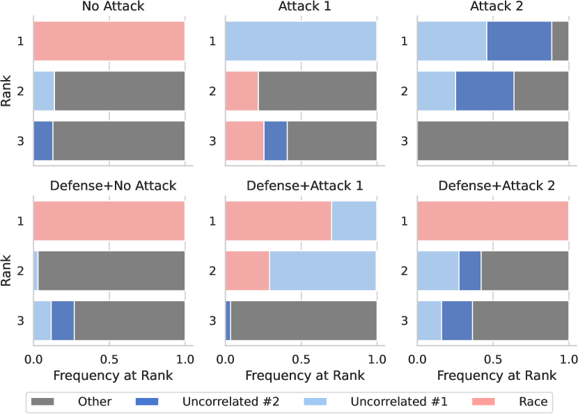
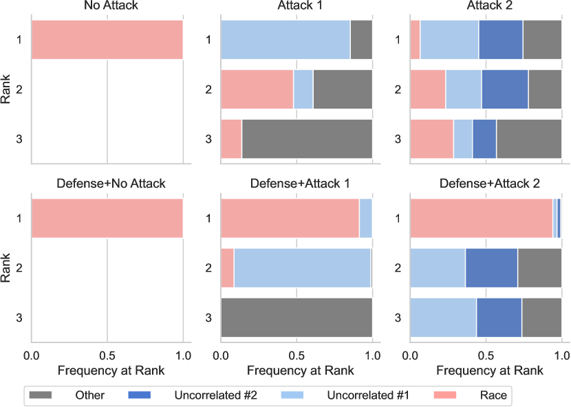
Figure 2: The top-3 most important features identified by LIME (left) and SHAP (right) with and without the defense on the COMPAS task. Our defense mitigates the attack and demonstrates that ACME attempted to conceal that race is an important factor in deciding the risk of recidivism. In the legend, “Other” represents any other COMPAS feature that is not “Race” or an “Uncorrelated” feature.

How effective is the attack?

We evaluate the efficacy of the attack with several metrics, expanding on its original evaluation (Slack et al. 2020). The classifier $f$ should be accurate on in-distribution data ($\text{fidelity}_{f}$) as given by Eq. (10)

$$\text{fidelity}_{f}(\bm{\mathcal{X}})=\frac{1}{|\bm{\mathcal{X}}|}\sum_{\mathbf{x}_{i}\in\bm{\mathcal{X}}}\llbracket f(\mathbf{x}_{i})=f_{\text{actual}}(\mathbf{x}_{i})\rrbracket$$ (10)

where

$$f_{\text{actual}}(\mathbf{x}_{i})=\begin{cases}f_{\text{biased}}(\mathbf{x}_{i})&\text{if attack is deployed}\\ f(\mathbf{x}_{i})&\text{otherwise}\end{cases}$$ (11)

When the attack is deployed, we can evaluate the quality of $d{}$ ($\text{fidelity}_{d{}}$) as the balanced accuracy between samples from $\bm{\mathcal{X}}$ and $\bm{\mathcal{X}}^{\text{(}g\text{)}{}}$ as in Eq. (12)

$$\begin{split}&\text{fidelity}_{d{}}(\bm{\mathcal{X}}\cup\bm{\mathcal{X}}^{(g)})=\\ &\frac{1}{2}\bigg{(}\frac{1}{|\bm{\mathcal{X}}|}\sum_{\mathbf{x}_{i}\in\bm{\mathcal{X}}}\llbracket d{}(\mathbf{x}_{i}){=}1\rrbracket{+}\frac{1}{|\bm{\mathcal{X}}^{(g)}|}\sum_{\mathbf{x}_{i}\in\bm{\mathcal{X}}^{(g)}}\llbracket d{}(\mathbf{x}_{i}){=}0\rrbracket\bigg{)}.\end{split}$$ (12)

To quantify the degree that $g$ is “fooled,” we compare the feature contributions to the features used by $f_{\text{actual}}$ from a feature-selectivity perspective. The features used by $f_{\text{actual}}$ can be split into selected ($\mathcal{F}_{\text{selected}}$) and unselected ($\mathcal{F}_{\neg{}\text{selected}}$) features. In turn, we can estimate the fidelity of $g$ as Eq. (13)

$$\begin{split}\text{fidelity}_{g}(\bm{\mathcal{X}}){=}\frac{1}{F{\cdot}|\bm{\mathcal{X}}|}\sum_{\mathbf{x}_{i}{\in}\bm{\mathcal{X}}}\rho\big{(}&\{F{-}1{\mid}j{\in}\mathcal{F}_{\text{selected}}\}{\cup}\\ &\{0{\mid}j{\in}\mathcal{F}_{\neg{}\text{selected}}\},\\ &\{r(\mathcal{E}_{i}^{-},a_{ij}){\mid}j{\in}\mathcal{F}\}\big{)}\end{split}$$ (13)

where $\mathcal{F}=\mathcal{F}_{\text{selected}}\cup\mathcal{F}_{\neg{}\text{selected}}$, $|\mathcal{F}|{=}F$, and $\rho$ gives the Spearman rank correlation coefficient between its two ordered arguments. Put simply, the correlation increases when features in $\mathcal{F}_{\text{selected}}$ are ranked higher than those in $\mathcal{F}_{\neg{}\text{selected}}$ by an explainer, i.e., explanations are more faithful.

As shown in Table 3, the attack is quite effective — fidelity_f remains high when the attack is active while fidelity_g decreases. This indicates that $d{}$ successfully toggles between $f_{\text{biased}}$ and $f_{\text{unbiased}}$, which is supported by the fidelity_d scores. Figure 2 qualitatively shows the efficacy of the attack on the COMPAS data set by visualizing the top-3 most frequent features in explanations.

Data Set	Attack	${N_{hl}}$	$g=$ LIME							$g=$ SHAP
			Fidelity				CAD- Detect	CAD- Defend		Fidelity				CAD- Detect	CAD- Defend
			${f}$	${d{}}$	${g}$	${h}$	$\Delta_{\text{cdf}}$	$\text{inf}_{g}$	$\text{fid}_{f}$	${f}$	${d{}}$	${g}$	${h}$	$\Delta_{\text{cdf}}$	$\text{inf}_{g}$	$\text{fid}_{f}$
COMPAS	✗	–	1.00	–	0.31	0.93	0.11	0.00	0.31	1.00	–	0.29	0.99	-0.02	0.00	0.29
	✓	1	0.99	0.99	0.23	0.81	0.30	0.05	0.30	0.93	0.82	0.24	0.77	0.20	0.02	0.28
	✓	2	0.99	0.99	0.10	0.80	0.30	0.00	0.31	0.91	0.82	0.24	0.77	0.25	0.01	0.26
German Credit	✗	–	1.00	–	0.27	0.78	0.07	0.00	0.27	1.00	–	0.24	0.86	-0.05	0.00	0.27
	✓	1	1.00	0.99	0.18	0.70	0.18	0.00	0.27	0.83	0.71	0.12	0.61	0.12	0.00	0.27
CC	✗	–	1.00	–	0.21	0.80	0.09	0.00	0.16	1.00	–	0.08	0.85	0.00	0.00	0.20
	✓	1	1.00	0.99	0.16	0.79	0.12	0.01	0.20	0.97	0.85	0.07	0.79	0.13	0.01	0.19
	✓	2	1.00	0.99	0.17	0.79	0.12	0.00	0.31	0.99	0.85	0.07	0.77	0.12	0.00	0.30

Table 3: The (in)fidelity and $\Delta_{\text{cdf}}$ scores of the attack and defense across the real-world data sets when KNN-CAD is used as $h$. $N_{hl}$ is the number of harmless features used by $f_{\text{unbiased}}$ and is unspecified when no attack is deployed. See the text for the differing definitions of fidelity for each algorithm. We abbreviate $\text{infidelity}_{{\texttt{CAD-Defend}}{},g}$ as $\text{inf}_{g}$ and $\text{fidelity}_{{\texttt{CAD-Defend}}{},f}$ as $\text{fid}_{f}$. Our approach successfully detects the scaffolding attack while maintaining explanation fidelity for both explainers.

Can we detect the attack?

We introduce metrics to evaluate $h$ and CAD-Detect in their ability to detect attacks. Here, $d_{\text{actual}}$ is $d{}$ when a scaffolding attack is deployed and a dummy function that returns ‘1’ otherwise. The ability of $h$ to model $\mathbb{P}(f(\mathbf{x}_{i}){\mid}\mathbf{x}_{i})$ is given by the weighted mean-square-error of $h$ and $d_{\text{actual}}$ (fidelity_h) as in Eq. (14)

$$\begin{split}\text{fidelity}_{h}&(\bm{\mathcal{X}}{\cup}\bm{\mathcal{X}}^{(g)})=\\ 1-\frac{1}{2}\bigg{(}&\frac{1}{|\bm{\mathcal{X}}|}\sum_{\mathbf{x}_{i}\in\bm{\mathcal{X}}}\left(d_{\text{actual}}(\mathbf{x}_{i}){-}h(\mathbf{x}_{i})\right)^{2}+\\ &\frac{1}{|\bm{\mathcal{X}}^{(g)}|}\sum_{\mathbf{x}_{i}\in\bm{\mathcal{X}}^{(g)}}\left(d_{\text{actual}}(\mathbf{x}^{(g)}_{i}){-}h(\mathbf{x}^{(g)}_{i})\right)^{2}\bigg{)}\end{split}$$ (14)

where $h(\cdot)$ is shorthand for $h$.score_samples$(\{\cdot\})$. Since $h$ gives probabilities, the error term is bounded to the range $[0,1]$ which we subtract from ‘1’ in order for the score to be interpreted as fidelity. To evaluate the quality of CAD-Detect, we compare the areas between the cumulative distributions of scores derived from $\bm{\mathcal{X}}^{\text{(}g\text{)}{}}$ and $\bm{\mathcal{X}}$ as described in Algorithm 3: $\Delta_{\text{cdf}}:=a_{\text{test}}^{\text{(}g\text{)}{}}-a_{\text{test}}$. This score should be higher if there is an attack deployed and lower otherwise.

Across all experiments, we use KNN-CAD as $h$. Our approach is able to detect every attack without false positives when $\tau_{\text{global}}\in[0.00,0.12]$ for SHAP and $\tau_{\text{global}}\in[0.11,0.12]$ for LIME. There is a trade-off in fidelity_h and fidelity_d — the more off-manifold the perturbations are, the harder it is to fit $\mathbb{P}(f(\mathbf{x}_{i})\mid\mathbf{x}_{i})$ (without an attack), whereas it is harder to fit $d{}$ when the perturbations are more on-manifold. The more principled game-theoretic perturbation scheme of SHAP demonstrably improves on that of LIME, yet it still can be gamed adversarially. Furthermore, a higher $\Delta_{\text{cdf}}$ without an attack deployed is indicative of more perturbed samples being off-manifold — discriminating attacks using SHAP has a far greater margin between $\Delta_{\text{cdf}}$ scores than LIME.

Can we “unfool” explainers?

In order for an explainer to be “unfooled,” it should produce explanations that 1) agree with its own explanations without an attack present and 2) agree with the feature selection by the black box algorithm. We propose $\text{infidelity}_{{\texttt{CAD-Defend}}{},g}$ to quantify how well CAD-Defend accomplishes the former goal. This metric measures the disagreement of the explanations when using CAD-Defend to those only using $g$ as in Eq. (15)

$$\begin{split}\text{infi}&\text{delity}_{{\texttt{CAD-Defend}}{},g}(\bm{\mathcal{X}})=\\ &\frac{1}{F\cdot|\bm{\mathcal{X}}|}\sum_{\mathbf{x}_{i}\in\bm{\mathcal{X}}}\sum_{(a^{(g)}_{ij},a^{(h)}_{ij})\in(\mathcal{E}^{(g)}_{i},\mathcal{E}^{(h)}_{i})}(a^{(g)}_{ij}-a^{(h)}_{ij})^{2}\end{split}$$ (15)

where $\mathcal{E}^{\text{(}g\text{)}{}}_{i}$ is the explanation from $g$ without an attack, $\mathcal{E}^{\text{(}h\text{)}{}}_{i}$ is the explanation when $h$ is used for defense during an attack, and $a_{ij}^{(*)}$ is as defined in Section 2. To evaluate against the true feature selection of $f_{\text{actual}}$, we use the same metric definition as $\text{fidelity}_{g}$ and refer to it as $\text{fidelity}_{{\texttt{CAD-Defend}}{},f}$.

The infidelity scores in Table 3 are near-zero across all tasks, demonstrating that our defense has very little disagreement with the explainer $g$ when $g$ is not under attack. In addition, the $\text{fidelity}_{{\texttt{CAD-Defend}}{},f}$ scores exceed those of $\text{fidelity}_{g}$ for all experiments when an attack is deployed and are close to $\text{fidelity}_{g}$ without an attack. A final piece of evidence that our defense mitigates the attack is shown in Figure 2 — comparing the top-3 most important features with and without the defense confirms that the defense is highly successful. See Appendix E for the same figure with the remaining explainers and data sets.

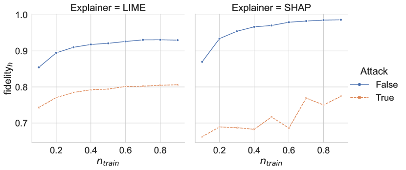
Figure 3: Sample-efficiency of KNN-CAD on the COMPAS data set when using LIME and SHAP as $g$ — fidelity_h is plotted as a function of the training proportion of the COMPAS data ($n_{\text{train}}$).

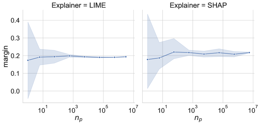
Figure 4: Sample-efficiency of CAD-Detect on the COMPAS data set when using LIME and SHAP as $g$ — the margin between the $\Delta_{cdf}$ scores with and without an attack is plotted as a function of the number of explainer perturbations ($n_{p}$).

Sample Efficiency

We evaluate the training sample-efficiency of our approach. Figure 3 plots fidelity_h as a function of the training proportion of the COMPAS data when using LIME and SHAP as $g$. Because of the strong inductive bias and nonparametric nature of KNN-CAD, the algorithm hardly degrades in performance even when 10% of the data is in use. This in part indicates the sample-efficiency of the CAD-Detect and CAD-Defend algorithms when KNN-CAD is used. We also evaluate the sample-efficiency of CAD-Detect on the COMPAS data set when using LIME and SHAP as $g$. The margin between the $\Delta_{\text{cdf}}$ scores with and without an attack is plotted as a function of the number of explainer perturbations, $n_{p}$. The main benefit of increasing $n_{p}$ is to increase the consistency of the detection score. When $n_{p}>1,000$ the variance tapers off for both explainers, which is just a small percentage of the millions of explainer-generated perturbations when all test set samples are explained. These findings are quite notable as the complexity bottleneck is due to querying $f$ as discussed in Section 3.

Additional Analyses

We include analyses of the hyperparameters of the three core algorithms, KNN-CAD, CAD-Detect and CAD-Defend, in Appendix F.

5 Discussion

In this work, we introduced several novel algorithms to defend against adversarial attacks on perturbation-based post hoc explainers: KNN-CAD for conditional anomaly detection, CAD-Detect for attack detection, and CAD-Defend to improve the fidelity of explanations when under attack. We rigorously formalized the attack and defense models, as well as introduced new quantitative metrics to evaluate the quality of the attack and defense. Our approach demonstrably mitigated the scaffolding attack across several real-world high-stakes data sets. The results indicate that the defense of SHAP is easier than LIME due to its more realistic data perturbations.

A limitation to consider is that the realistic samples used in the training set for the defense algorithm can be expensive or difficult to collect. Moreover, in realistic scenarios, an API to a black box may be costly to query with the perturbed samples generated by explainers. In practice, explainer queries should be rate-limited so as to not arise suspicion from the auditee. On this note, we do not consider the case when the adversary irregularly deploys the attack. We point to (Schneider, Meske, and Vlachos 2022) which characterizes this attack and demonstrates that explanations that are infrequently manipulated can be difficult to detect. In addition, we considered the case of an adversary masking malicious behavior. However, the motivation for such behavior could arise for privacy reasons or to protect intellectual property from model extraction attacks (Tramèr et al. 2016).

We analyze and alleviate a single shortcoming of post hoc explainers. However, the explainers we consider have also been shown to be inconsistent, unfaithful, and intractable (Krishna et al. 2022; Bordt et al. 2022; den Broeck et al. 2021; Garreau and von Luxburg 2020; Carmichael and Scheirer 2021a, b). Consequently, a potential source of negative societal impact in this work arises from practitioners overtrusting post hoc explainers (Kaur et al. 2020). Nevertheless, our study demonstrates that the explainers backed with our proposed defense not only detect adversarial behavior but also faithfully identify the most important features in decisions. Moreover, if an explainer is not to be trusted, our approach can at least exploit it to identify misbehaving algorithms. In future work, the ramifications of an adversarial organization caught red-handed should be explored in the context of existing regulatory guidelines.

Supplemental Material

We highly recommend that this supplemental material be viewed digitally.

Appendix A Selection of $f_{\text{biased}}$ and $f_{\text{unbiased}}$

The following details the specifics of the rule-based $f_{\text{biased}}$ and $f_{\text{unbiased}}$ classifiers across the real-world data sets.

• COMPAS

  1. $f_{\text{biased}}$: high-risk if race is African American, otherwise low-risk. $f_{\text{unbiased}}$: high-risk if uncorrelated_feature_1 is 1, otherwise low-risk.

  2. $f_{\text{biased}}$: high-risk if race is African American. $f_{\text{unbiased}}$: high-risk if uncorrelated_feature_1 XOR uncorrelated_feature_2 is 1, otherwise low-risk.

• German Credit

  1. $f_{\text{biased}}$: good customer if gender is male, otherwise bad customer. $f_{\text{unbiased}}$: good customer if LoanRateAsPercentOfIncome is greater than the mean of LoanRateAsPercentOfIncome in the training set, otherwise bad customer.

• Communities & Crime

  1. $f_{\text{biased}}$: low violent crime rate if racePctWhite is above average, otherwise high. $f_{\text{unbiased}}$: low violent crime rate if uncorrelated_feature_1, otherwise high.

  2. $f_{\text{biased}}$: low violent crime rate if racePctWhite is above average, otherwise high. $f_{\text{unbiased}}$: low violent crime rate if (uncorrelated_feature_1 is greater than 0.5) XOR (uncorrelated_feature_2 is greater than -0.5), otherwise high.

Appendix B Reproducibility

The following details the hyperparameters, hardware and software used across all experiments. See Appendix D for a discussion of nondeterminism in experiments and results with error bars over multiple trials. The code is available at the public repository listed in the manuscript.

Hyperparameters

The hyperparameters used for the $d{}$, explainers, and defense algorithms are shown in Table 5, Table 7, and Table B3, respectively. All data is normalized using standard z-score normalization based on the mean and standard deviation of the training split of data.

Hyperparameter	Value
n_estimators	100
criterion	gini
min_samples_split	None
min_samples_leaf	2
min_weight_fraction_leaf	1
max_features	auto
max_leaf_nodes	None
min_impurity_decrease	0.0
bootstrap	True
oob_score	False
max_samples	None

Table B1: Hyperparameters of $d{}$ used across all experiments. In general, the default scikit-learn hyperparameter values are selected. See the scikit-learn documentation of RandomForestClassifier for details of each hyperparameter.

Explainer	Hyperparameter	Value
LIME	kernel_width	$F\times 0.75$
	kernel	exponential
	feature_selection	auto
	num_features	10
	num_samples	5000
	discretize_continuous	False
SHAP	background_distribution	k-means ($k=20$)
	nsamples	auto
	l1_reg	auto

Table B2: Explainer hyperparameters used across all experiments. In general, the default explainer hyperparameters are used. See the documentation of LIME and SHAP for the meaning of each hyperparameter.

Algorithm	Hyperparameter	Value
KNN-CAD	$k$	15
	$\phi$	max
	$\epsilon$	0.1
	distance	minkowski
	$p$	1
CAD-Detect	$\tau_{\text{global}}$	$[0.11,0.12]$
	$n_{\text{train}}$	$0.9\times|\bm{\mathcal{D}}|$
	$n_{p}$	$\min(|\bm{\mathcal{X}}^{(g)}|,|\bm{\mathcal{D}}_{\text{train}}|\times 10)$
CAD-Defend	$\tau$	0.75

Table B3: Defense algorithm hyperparameters used for each experiment unless otherwise specified.

Hardware and Software

All experiments were run on a machine with the following relevant hardware and software specifications:

• Hardware

  • AMD Ryzen 9 5950X (code is CPU only)

  • 64 GiB DDR4 RAM

• Software

  • Manjaro Linux 21.2.6 (Qonos)

  • Python 3.9.13

    • ipykernel==6.7.0

    • jupyter-client==7.1.2

    • jupyter-core==4.9.1

    • lime==0.2.0.1

    • matplotlib==3.5.1

    • numpy==1.21.0

    • pandas==1.4.0

    • scikit-learn==1.0.2

    • scipy==1.7.3

    • seaborn==0.11.2

    • shap==0.40.0

Appendix C Data

COMPAS

The COMPAS data set is available for download on the ProPublica GitHub repository. The data set is provided by ProPublica without a listed license but external analysis of the data is encouraged. The data set does not contain offensive content and does not contain personally identifiable information — all data is collected from public records of the defendants in Broward County, Florida.

https://github.com/propublica/compas-analysis

German Credit

The German Credit data set is available through the UCI machine learning repository. UCI-donated data sets are licensed under the Creative Commons Attribution 4.0 International license (CC BY 4.0). UCI-donated data sets also do not have personally-identifiable information. The data set does not contain offensive content.

https://archive.ics.uci.edu/ml/datasets/statlog+(german+credit+data)

Communities & Crime

The Communities & Crime data set is available through the UCI machine learning repository. UCI-donated data sets are licensed under the Creative Commons Attribution 4.0 International license (CC BY 4.0). UCI-donated data sets also do not have personally-identifiable information. The data set does not contain offensive content.

https://archive.ics.uci.edu/ml/datasets/communities+and+crime

Appendix D Error Bars

While our core algorithm, KNN-CAD, is deterministic, there is randomness in experiments owing to the perturbation processes of LIME and SHAP. $f_{\text{biased}}$ is deterministic as it is rule-based and operates on feature values that do not change between trials. While $f_{\text{unbiased}}$ is deterministic, its predictions are nondeterministic due to the random generation process of the uncorrelated features used in the COMPAS and Communities & Crime tasks. Furthermore, $f$ is not deterministic as $d{}$ is a function of a random forest. In turn, both CAD-Detect and CAD-Defend are nondeterministic. We report the results with standard deviations across 10 trials in Table D4.

$g$	Data Set	$N_{hl}$	Fidelity				CAD- Detect	CAD- Defend
			${f}$	${d{}}$	${g}$	${h}$	$\Delta_{\text{cdf}}$	$\text{inf}_{g}$	$\text{fid}_{f}$
LIME	CO	–	1.00${\pm}$0.00	–	0.31${\pm}$0.01	0.93${\pm}$0.01	0.11${\pm}$0.01	0.00${\pm}$0.00	0.31${\pm}$0.01
		1	0.99${\pm}$0.01	0.99${\pm}$0.01	0.23${\pm}$0.01	0.81${\pm}$0.01	0.30${\pm}$0.02	0.05${\pm}$0.01	0.30${\pm}$0.01
		2	0.99${\pm}$0.01	0.99${\pm}$0.01	0.10${\pm}$0.01	0.80${\pm}$0.01	0.30${\pm}$0.01	0.00${\pm}$0.00	0.31${\pm}$0.01
	GC	–	1.00${\pm}$0.00	–	0.27${\pm}$0.01	0.78${\pm}$0.01	0.07${\pm}$0.02	0.00${\pm}$0.00	0.27${\pm}$0.01
		1	1.00${\pm}$0.00	0.99${\pm}$0.01	0.18${\pm}$0.01	0.70${\pm}$0.02	0.18${\pm}$0.02	0.00${\pm}$0.00	0.27${\pm}$0.01
	CC	–	1.00${\pm}$0.00	–	0.21${\pm}$0.01	0.80${\pm}$0.01	0.09${\pm}$0.01	0.00${\pm}$0.00	0.16${\pm}$0.01
		1	1.00${\pm}$0.00	0.99${\pm}$0.01	0.16${\pm}$0.01	0.79${\pm}$0.02	0.12${\pm}$0.01	0.01${\pm}$0.00	0.20${\pm}$0.01
		2	1.00${\pm}$0.00	0.99${\pm}$0.01	0.17${\pm}$0.02	0.79${\pm}$0.03	0.12${\pm}$0.01	0.00${\pm}$0.00	0.31${\pm}$0.01
SHAP	CO	–	1.00${\pm}$0.00	–	0.29${\pm}$0.01	0.99${\pm}$0.01	-0.02${\pm}$0.01	0.00${\pm}$0.00	0.29${\pm}$0.01
		1	0.93${\pm}$0.01	0.82${\pm}$0.02	0.24${\pm}$0.01	0.77${\pm}$0.02	0.20${\pm}$0.01	0.02${\pm}$0.00	0.28${\pm}$0.01
		2	0.91${\pm}$0.01	0.82${\pm}$0.02	0.24${\pm}$0.01	0.77${\pm}$0.02	0.25${\pm}$0.01	0.01${\pm}$0.00	0.26${\pm}$0.02
	GC	–	1.00${\pm}$0.00	–	0.24${\pm}$0.01	0.86${\pm}$0.01	-0.05${\pm}$0.00	0.00${\pm}$0.00	0.27${\pm}$0.02
		1	0.83${\pm}$0.02	0.71${\pm}$0.02	0.12${\pm}$0.01	0.61${\pm}$0.02	0.12${\pm}$0.01	0.00${\pm}$0.00	0.27${\pm}$0.02
	CC	–	1.00${\pm}$0.00	–	0.08${\pm}$0.01	0.85${\pm}$0.01	0.00${\pm}$0.01	0.00${\pm}$0.00	0.20${\pm}$0.01
		1	0.97${\pm}$0.01	0.85${\pm}$0.02	0.07${\pm}$0.00	0.79${\pm}$0.01	0.13${\pm}$0.01	0.01${\pm}$0.00	0.19${\pm}$0.01
		2	0.99${\pm}$0.01	0.85${\pm}$0.02	0.07${\pm}$0.00	0.77${\pm}$0.02	0.12${\pm}$0.01	0.00${\pm}$0.00	0.30${\pm}$0.01

Table D4: The (in)fidelity and $\Delta_{\text{cdf}}$ scores of the attack and defense across the real-world data sets when KNN-CAD is used as $h$. The scores are reported across 10 trials with standard deviations. The data sets are abbreviated as follows: COMPAS (CO), German Credit (GC), Communities & Crime (CC). $N_{hl}$ is the number of harmless features used by $f_{\text{unbiased}}$ and is unspecified when no attack is deployed. See the text for the differing definitions of fidelity for each algorithm. We abbreviate $\text{infidelity}_{{\texttt{CAD-Defend}}{},g}$ as $\text{inf}_{g}$ and $\text{fidelity}_{{\texttt{CAD-Defend}}{},f}$ as $\text{fid}_{f}$. Our approach successfully detects the scaffolding attack while maintaining explanation fidelity for both explainers.

Appendix E Additional Top-3 Feature Plots

The following figures show the top-3 most important features as identified by LIME and SHAP with and without the defense across all attack scenarios: Figures E1-E4. For the Communities and Crime attack with LIME and $N_{hl}=1$, our method is able to increase the importance of the sensitive feature in the second rank, but not the first. However, CAD-Detect is still able to detect that $f$ is acting adversarially as shown in Table D4. Otherwise, our approach is successful.

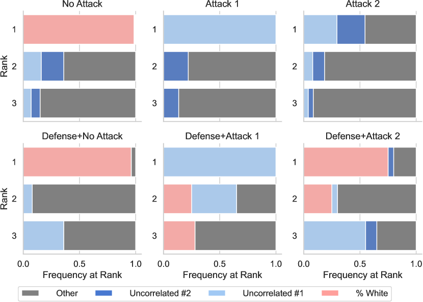
Figure E1: The top-3 most important features identified by LIME with and without the defense on the Communities & Crime task. Our defense improves upon the first attack and mitigates the second attack and demonstrates that ACME likely attempted to conceal that race is frequently factored into violent crime prediction.

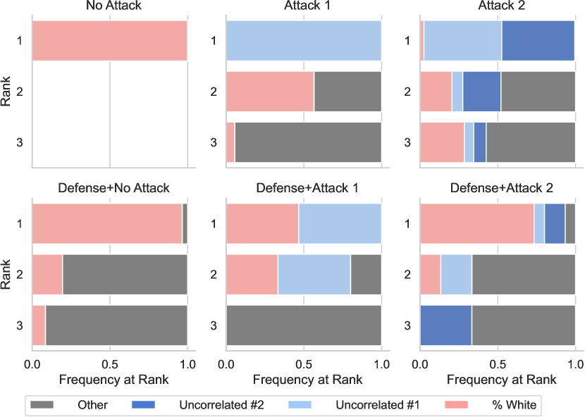
Figure E2: The top-3 most important features identified by SHAP with and without the defense on the Communities & Crime task. Our defense improves upon the first attack and mitigates the second attack and demonstrates that ACME likely attempted to conceal that race is frequently factored into violent crime prediction.

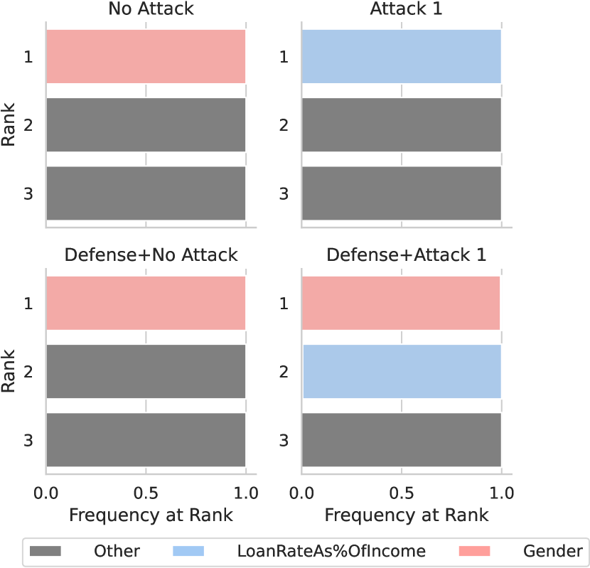
Figure E3: The top-3 most important features identified by LIME with and without the defense on the Boston Credit task. Our defense mitigates the attack and demonstrates that ACME attempted to conceal that gender is frequently factored into credit risk.

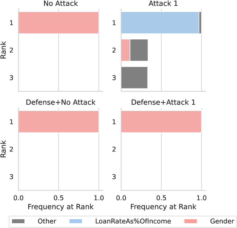
Figure E4: The top-3 most important features identified by SHAP with and without the defense on the Boston Credit task. Our defense mitigates the attack and demonstrates that ACME attempted to conceal that gender is frequently factored into credit risk.

Appendix F Additional Analyses

Hyperparameter Analysis

Here, we conduct an analysis of the KNN-CAD hyperparameters $\phi$, $k$, and Minkowski distance $p$ on the Communities & Crime data set — see Figures F5 and F6. Ideally, KNN-CAD maximizes the difference between $\Delta_{cdf}$ when the attack is deployed and $\Delta_{cdf}$ when no attack is present. We refer to this difference as the margin. The margin is visualized as a function of the same hyperparameters in Figures F7 and F8. The $\Delta_{cdf}$ scores in both cases decrease as $k$ increases. Irrespective of $\phi$, $\Delta_{cdf}$ is the same when $k=1$. However, $\Delta_{cdf}$ scores peak when $k>1$. There is very little difference in $\Delta_{cdf}$ or the margin for different values of $p$ (although $p=1$ results in a slightly higher peak margin). The margin is maximized with lower values of $k$. The selection of $\phi$ generally has the affect of modulating the mean value of $\Delta_{cdf}$. With the train split, $\phi=\texttt{min}$ results in a abnormally low mean $\Delta_{cdf}$ simply because the neighbors are of the same split. All values of $\phi$ result in a similar margin, but $\phi=\texttt{min}$ performs best across all values of $k$, $p$, and split. An oddity is that $\phi=\texttt{min}$ begins to fail for SHAP on the train split with $p=2$ and $k>50$ – we presume this occurs because $\phi=\texttt{min}$ is a brittle estimator compared to the mean or median. All of these observations hold between both the train and test splits used to estimate $\Delta_{cdf}$ in the CAD-Detect algorithm. Owing to its more principled perturbation scheme, the margin when using SHAP is ${\sim}5{\times}$ greater than that of LIME in general.

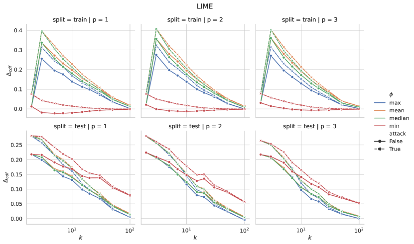
Figure F5: Analysis of hyperparameters of KNN-CAD when performing detection (CAD-Detect) with the LIME explainer. The $\Delta_{cdf}$ score is reported as a function of $k$ on the Communities & Crime dataset. The ideal hyperparameters maximize the difference between $\Delta_{cdf}$ when the attack is deployed and is not.

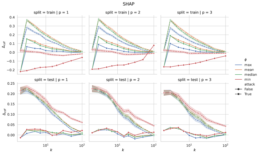
Figure F6: Analysis of hyperparameters of KNN-CAD when performing detection (CAD-Detect) with the SHAP explainer. The $\Delta_{cdf}$ score is reported as a function of $k$ on the Communities & Crime dataset. The ideal hyperparameters maximize the difference between $\Delta_{cdf}$ when the attack is deployed and is not.

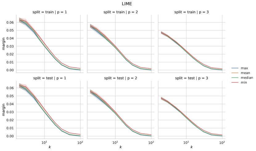
Figure F7: Analysis of hyperparameters of KNN-CAD when performing detection (CAD-Detect) with the LIME explainer. The margin is reported as a function of $k$ on the Communities & Crime dataset.

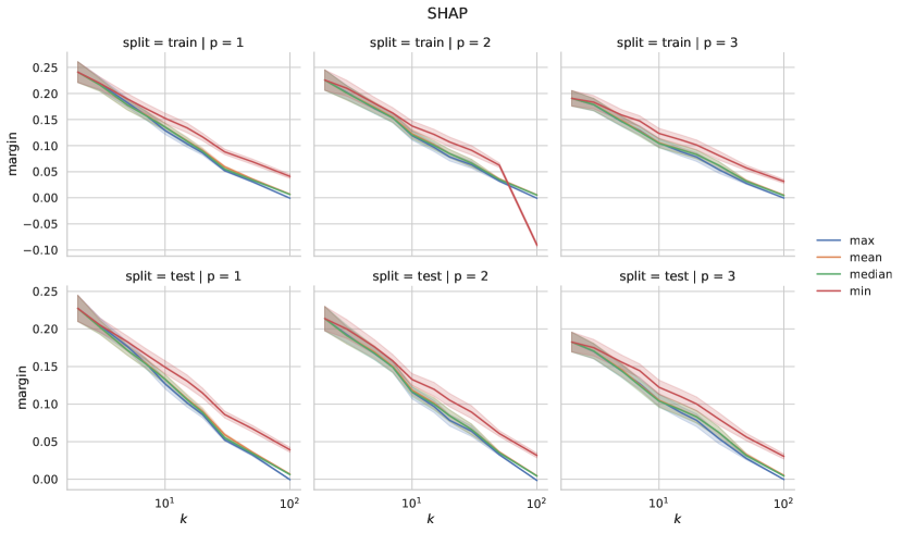
Figure F8: Analysis of hyperparameters of KNN-CAD when performing detection (CAD-Detect) with the SHAP explainer. The margin is reported as a function of $k$ on the Communities & Crime dataset.

Appendix G Further Delineating the Problem Scenario Formalism

In this appendix, we elucidate our formalization of the attack and defense scenarios using a rolling example. Please refer back to Figure 1 in the main text for a visual aid of the scenario.

The potential adversary, ACME Corporation, has an automated decision-making system $f$. The system $f$ makes decisions on behalf of its users in potentially high-stakes applications and is a black box. The data (denoted by $\bm{\mathcal{X}}$) comprises $F$ features, some of which may be protected (or sensitive) according to regulation or law. To ensure that each algorithm $f$ deployed by ACME meets regulatory compliance, an auditor devises a strategy to understand the decision-making process of $f$.

In this work, it is considered that $f$ fails to meet compliance if it uses a protected feature to make high-stakes decisions, and if $f$ behaves adversarially depending on whether it is being audited. To verify that ACME meets such compliance, the auditor uses an explainer, $g$, that provides a set of feature contributions $\{a_{ij}\}_{j}^{F}$ for the $i^{\text{th}}$ data sample $\mathbf{x}_{i}$. Each contribution $a_{ij}$ provides the additive contribution of feature $j$ to the prediction value of $f(\mathbf{x}_{i})$. In the main text, the explainer $g$ produces explanations by optimizing the objective defined in Eq. (1). Since the explainers are perturbation-based, a set of perturbed data samples are generated when explaining data. We denote this set of perturbations as $\bm{\mathcal{X}}^{(g)}$ and note that it is derived from $\bm{\mathcal{X}}$. The auditor thereafter can determine if ACME met compliance if the features were not used in a way that violates regulations.

Unfortunately, ACME may act in an adversarial manner and attempt to hide the decision-making process of its algorithm $f$. For instance, a scaffolding attack may be employed as described in Section 2 and Eq. (2) – if ACME detects that an explainer $g$ is querying $f$, it can toggle from its biased model to one that is unbiased, thwarting the audit. The general objective of an attack is laid out in Eq. (4). In the equation, recall that $\mathcal{E}_{i}^{-}=\mathcal{E}_{i}^{\text{sensitive}}\cup\mathcal{E}_{i}^{\text{harmless}}=g(\mathbf{x}_{i};f)$ is an ordered set of feature contributions for the $i^{\text{th}}$ data sample, and $\mathcal{E}_{i}^{\text{sensitive}}$ and $\mathcal{E}_{i}^{\text{harmless}}$ are the subsets of $\mathcal{E}_{i}^{-}$ corresponding to the sensitive and harmless features, respectively. With that established, the objective is to simultaneously minimize the error between the ground truth, $y_{i}$, and the predictions of $f$ (as is done in normal supervised learning), but to also minimize the number of highly-ranked contributions of sensitive features. Put even simpler, an adversarial ACME wants to retain the fidelity of its algorithm $f$ while hiding the fact that sensitive features are important to the decision-making process.

In this work, we consider that an adversarial ACME employs the scaffolding attack. The objective of the attack is defined in Eq. (5). Let us assume that we, as an oracle, know whether a data sample originated from normal data ($\bm{\mathcal{X}}$) or from the perturbations of an explainer $g$ ($\bm{\mathcal{X}}^{(g)}$). Let $t_{i}\in\mathcal{T}$ denote this information, i.e., $t_{i}=1$ if $\mathbf{x}_{i}\in\bm{\mathcal{X}}^{(g)}$ and $t_{i}=0$ otherwise. With this established, ACME desires to use a biased algorithm $f_{\text{biased}}$ whenever $t_{i}=0$ and an unbiased algorithm $f_{\text{unbiased}}$ when $t_{i}=0$. In the scaffolding approach, this is solved by selecting the out-of-distribution detector, $d{}$, that minimizes Eq. (5). In short, the adversary aims to use an unbiased predictor when it is audited in order to meet regulatory compliance.

As discussed, the auditor can use $g$ to provide explanations of the decisions of $f$ to see if the way features were used violates regulatory compliance. However, we did not establish how the auditor can verify that $f$ does not change its decision-making process when being audited. Without a defense approach, ACME can hide their decision-making processes from the auditor as-is. We provide an approach to the detection and defense of the scaffolding attack, the former detecting whether the attack is deployed and the latter mitigating the attack so that explanations are not altered. The problem can be understood by considering the conditional probability mass function $p(f(\mathbf{x}_{i})\mid\mathbf{x}_{i})$. The distribution indicates the likelihood of $f$ predicting some outcome given that the input is $\mathbf{x}_{i}$, which is necessary because the attacker changes its prediction (e.g., biased or unbiased) based on the input (e.g., on- or off-manifold). Based on the probability measure of individual samples, i.e., $\mathbb{P}(f(\mathbf{x}_{i})\mid\mathbf{x}_{i})$, we can determine if the behavior of $f$ has changed – low-likelihood samples indicate that $f$ is likely behaving adversarially. In the defense approach, $p$ is estimated by a conditional anomaly detector $h$ that should optimize for the objective given by Eq. (6). Put simply, the goal of the defense is to learn the distribution of normal behavior of $f$. If $f$ is not acting normally (the conditional likelihood of predictions is below a threshold as in Eq. (3)), then we can perform both detection and explanation defense. Detection is performed as in Eq. (7) where we measure the distance between the distributions $p(f(\mathbf{x}_{i})\mid\mathbf{x}_{i})$ and $p(f(\mathbf{x}^{(g)}_{i})\mid\mathbf{x}^{(g)}_{i})$ – if the distribution of perturbed samples differs significantly from natural samples, then $f$ is likely acting adversarially for the explainer $g$. At this point, the auditor can determine whether ACME is complying with the audit and whether to trust the explanations of $g$ before further scrutiny.

For descriptions of the KNN-CAD and explanation defense approaches, please see “Detection, Defense and KNN-CAD” and Algorithms 1–4 in Section 3 of the main text.

Appendix H Additional Attack Vectors

It is possible that the attacker can detect whether multiple queries come from the same neighborhood consecutively. If so, the attacker can then exploit this information to always use the unbiased model. We can easily devise a solution to mitigate this attack that follows the defense approach. Simply, the queries that are made to $f$ can be reordered to alternate between neighborhoods. Since there are multiple samples that are being explained, there is in turn a neighborhood for each sample. By switching between multiple neighborhoods, this makes detecting neighborhoods a substantially more difficult problem. Naturally, since the number of explainer perturbations outnumber the samples representing normality, one might wonder if there is a tractable number of samples in order for the defense to be undetected in this attack vector. In Appendix F, we demonstrate that our approach is extremely sample-efficient – a small percentage of the neighborhood samples are required to be confident in whether $f$ is behaving adversarially. To realize the defense against this attack vector, we modify Algorithms 3 and 4 to perform a shuffle stratified among the neighborhoods.

Appendix I Time and Space Complexities

Algorithm KNN-CAD.fit

Time: $\mathcal{O}(FN\log N)$ (construction of a ball tree) + $\mathcal{O}(N(k\log N+T_{f}(F)))$ (KNN-CAD.score_samples) + $\mathcal{O}(N\log N)$ (sorting the scores) = $\mathcal{O}(N(F\log N+k\log N+T_{f}(F)))$.

Space: $\mathcal{O}(FN)$ (construction of a ball tree) + $\mathcal{O}(N(k+S_{f}(F)))$ (KNN-CAD.score_samples) + $\mathcal{O}(N)$ (the scores) = $\mathcal{O}(N(F+k+S_{f}(F)))$.

Algorithm KNN-CAD.score_samples

Time: $\mathcal{O}(N\,T_{f}(F))$ (calling $f$ for each sample) + $\mathcal{O}(kN\log N)$ (querying the $k$ nearest neighbors for each sample) + $\mathcal{O}(Nk)$ (computing scores from neighbors and classes for each sample) = $\mathcal{O}(N(k\log N+T_{f}(F)))$. In practice where $T_{f}(F)\gg k\log N$ is likely, e.g., with DNNs, the time complexity is $\mathcal{O}(NT_{f}(F))$. If we are provided with pre-computed predictions, the time complexity is $\mathcal{O}(kN\log N)$.

Space: $\mathcal{O}(N\,S_{f}(F))$ (calling $f$ for each sample) + $\mathcal{O}(kN)$ (querying the $k$ nearest neighbors for each sample) + $\mathcal{O}(N)$ (computing scores from neighbors and classes for each sample) = $\mathcal{O}(N(k+S_{f}(F)))$. In practice where $S_{f}(F)\gg k$ is likely, the space complexity is $\mathcal{O}(NS_{f}(F))$. If we are provided with pre-computed predictions, the space complexity is $\mathcal{O}(kN)$.

Algorithm CAD-Detect

Time: $\mathcal{O}(N(F\log N+k\log N+T_{f}(F)))$ (fitting KNN-CAD) + $\mathcal{O}(N(k\log N+T_{f}(F)))$ (scoring the test samples) + $\mathcal{O}(Nn_{p}(k\log(Nn_{p})+T_{f}(F)))$ (scoring the $n_{p}$ perturbations per test sample) + $\mathcal{O}(Nn_{p})$ (computing areas) = $\mathcal{O}(Nn_{p}(k\log(Nn_{p})+T_{f}(F)))$.

Space: $\mathcal{O}(N(F+k+S_{f}(F)))$ (fitting KNN-CAD) + $\mathcal{O}(N(k+S_{f}(F)))$ (scoring the test samples) + $\mathcal{O}(Nn_{p}(k+S_{f}(F)))$ (scoring the $n_{p}$ perturbations per test sample) + $\mathcal{O}(Nn_{p})$ (computing areas) = $\mathcal{O}(Nn_{p}(k+S_{f}(F)))$.

Algorithm CAD-Defend

Time: $\mathcal{O}(n_{p}(k\log n_{p}+T_{f}(F)))$ (scoring the $n_{p}$ perturbations for the test sample) + $\mathcal{O}(n_{p})$ (filtering and set operations) + $\mathcal{O}(R\,T_{{\texttt{CAD-Defend}}{}}(n_{p},k,F))$ (the algorithm is executed in $R$ recursions, with the same input size in the worst case) = $\mathcal{O}(Rn_{p}(k\log n_{p}+T_{f}(F)))$. In the worst case, all generated samples are abnormal and filtered, e.g., if the threshold is set too high or $h$ is fit poorly. In practice, fewer than $n_{p}$ samples are required at each recursion.

Space: $\mathcal{O}(n_{p}(k+S_{f}(F)))$ (scoring the $n_{p}$ perturbations for the test sample) + $\mathcal{O}(n_{p})$ (filtering and set operations) = $\mathcal{O}(n_{p}(k+S_{f}(F)))$. The space of only one recursion is necessary to consider.

References

- Abdukhamidov et al. (2022) Abdukhamidov, E.; Juraev, F.; Abuhamad, M.; and Abuhmed, T. 2022. Black-box and Target-specific Attack Against Interpretable Deep Learning Systems. In Asia Conference on Computer and Communications Security. ACM.
- Akpinar et al. (2022) Akpinar, N.-J.; Leqi, L.; Hadfield-Menell, D.; and Lipton, Z. 2022. Counterfactual Metrics for Auditing Black-Box Recommender Systems for Ethical Concerns. In Workshop on Responsible Decision Making in Dynamic Environments, International Conference on Machine Learning, ICML, volume 162 of Proceedings of Machine Learning Research. PMLR.
- Angwin et al. (2016) Angwin, J.; Larson, J.; Mattu, S.; and Kirchner, L. 2016. Machine bias: there’s software used across the country to predict future criminals. And it’s biased against blacks. https://www.propublica.org/article/machine-bias-risk-assessments-in-criminal-sentencing.
- Baniecki (2022) Baniecki, H. 2022. Adversarial Explainable AI. https://hbaniecki.com/adversarial-explainable-ai/. Accessed: 2022-11-29.
- Barredo Arrieta et al. (2020) Barredo Arrieta, A.; Díaz-Rodríguez, N.; Del Ser, J.; Bennetot, A.; Tabik, S.; Barbado, A.; Garcia, S.; Gil-Lopez, S.; Molina, D.; Benjamins, R.; Chatila, R.; and Herrera, F. 2020. Explainable Artificial Intelligence (XAI): Concepts, taxonomies, opportunities and challenges toward responsible AI. Information Fusion, 58: 82–115.
- Bordt et al. (2022) Bordt, S.; Finck, M.; Raidl, E.; and von Luxburg, U. 2022. Post-Hoc Explanations Fail to Achieve their Purpose in Adversarial Contexts. ACM Conference on Fairness, Accountability, and Transparency, 5.
- Buolamwini and Gebru (2018) Buolamwini, J.; and Gebru, T. 2018. Gender Shades: Intersectional Accuracy Disparities in Commercial Gender Classification. In Conference on Fairness, Accountability and Transparency, 77–91. PMLR.
- Carmichael and Scheirer (2021a) Carmichael, Z.; and Scheirer, W. J. 2021a. A Framework for Evaluating Post Hoc Feature-Additive Explainers. arXiv:2106.08376.
- Carmichael and Scheirer (2021b) Carmichael, Z.; and Scheirer, W. J. 2021b. On the Objective Evaluation of Post Hoc Explainers. arXiv:2106.08376.
- den Broeck et al. (2021) den Broeck, G. V.; Lykov, A.; Schleich, M.; and Suciu, D. 2021. On the Tractability of SHAP Explanations. In AAAI Conference on Innovative Applications of Artificial Intelligence, IAAI, 6505–6513. AAAI Press.
- Dua and Graff (2017) Dua, D.; and Graff, C. 2017. UCI Machine Learning Repository. http://archive.ics.uci.edu/ml. University of California, Irvine, School of Information and Computer Sciences.
- EU and Parliament (2016) EU, C. o. t.; and Parliament, E. 2016. Regulation (EU) 2016/679 of the European Parliament and of the Council of 27 April 2016 on the protection of natural persons with regard to the processing of personal data and on the free movement of such data, and repealing Directive 95/46/EC (General Data Protection Regulation). Official Journal of the European Union, L 119: 1–88.
- European Commission (2021) European Commission. 2021. Proposal for a regulation of the European Parliament and the Council: Laying down harmonised rules on Artificial Intelligence (Artificial Intelligence Act) and amending certain Union legislative acts. https://eur-lex.europa.eu/legal-content/EN/TXT/?uri=CELEX:52021PC0206.
- FICO (2018) FICO, F. I. C. 2018. FICO Explainable Machine Learning Challenge: Home Equity Line of Credit (HELOC) Dataset. https://community.fico.com/s/explainable-machine-learning-challenge.
- Garreau and von Luxburg (2020) Garreau, D.; and von Luxburg, U. 2020. Explaining the Explainer: A First Theoretical Analysis of LIME. In Chiappa, S.; and Calandra, R., eds., International Conference on Artificial Intelligence and Statistics, volume 108 of Proceedings of Machine Learning Research, 1287–1296. PMLR.
- Ghalebikesabi et al. (2021a) Ghalebikesabi, S.; Ter-Minassian, L.; DiazOrdaz, K.; and Holmes, C. C. 2021a. On locality of local explanation models. Advances in Neural Information Processing Systems, 34.
- Ghalebikesabi et al. (2021b) Ghalebikesabi, S.; Ter-Minassian, L.; DiazOrdaz, K.; and Holmes, C. C. 2021b. [OpenReview Discussion] On Locality of Local Explanation Models. In Beygelzimer, A.; Dauphin, Y.; Liang, P.; and Vaughan, J. W., eds., Advances in Neural Information Processing Systems.
- Hendrycks et al. (2021) Hendrycks, D.; Zhao, K.; Basart, S.; Steinhardt, J.; and Song, D. 2021. Natural Adversarial Examples. In Conference on Computer Vision and Pattern Recognition, 15262–15271. IEEE/Computer Vision Foundation.
- Kaur et al. (2020) Kaur, H.; Nori, H.; Jenkins, S.; Caruana, R.; Wallach, H.; and Wortman Vaughan, J. 2020. Interpreting Interpretability: Understanding Data Scientists’ Use of Interpretability Tools for Machine Learning. In Bernhaupt, R.; Mueller, F. F.; Verweij, D.; Andres, J.; McGrenere, J.; Cockburn, A.; Avellino, I.; Goguey, A.; Bjøn, P.; Zhao, S.; Samson, B. P.; and Kocielnik, R., eds., Conference on Human Factors in Computing Systems, 1–14. ACM.
- Krishna et al. (2022) Krishna, S.; Han, T.; Gu, A.; Pombra, J.; Jabbari, S.; Wu, S.; and Lakkaraju, H. 2022. The Disagreement Problem in Explainable Machine Learning: A Practitioner’s Perspective. arXiv:2202.01602.
- Lipton (2018) Lipton, Z. C. 2018. The Mythos of Model Interpretability. ACM Queue, 16(3): 30.
- Lundberg and Lee (2017) Lundberg, S. M.; and Lee, S.-I. 2017. A Unified Approach to Interpreting Model Predictions. In Guyon, I.; von Luxburg, U.; Bengio, S.; Wallach, H. M.; Fergus, R.; Vishwanathan, S. V. N.; and Garnett, R., eds., Conference on Neural Information Processing Systems, 4765–4774.
- McGregor (2021) McGregor, S. 2021. Preventing Repeated Real World AI Failures by Cataloging Incidents: The AI Incident Database. In AAAI Conference on Innovative Applications of Artificial Intelligence, IAAI, 15458–15463. AAAI Press.
- Miller and Brown (2018) Miller, D. D.; and Brown, E. W. 2018. Artificial Intelligence in Medical Practice: The Question to the Answer? The American Journal of Medicine, 131(2): 129–133.
- Noppel, Peter, and Wressnegger (2022) Noppel, M.; Peter, L.; and Wressnegger, C. 2022. Backdooring Explainable Machine Learning. arXiv:2204.09498.
- O’Neil (2016) O’Neil, C. 2016. Weapons of Math Destruction: How Big Data Increases Inequality and Threatens Democracy. Crown. ISBN 978-0-553-41883-5.
- Redmond and Baveja (2002) Redmond, M.; and Baveja, A. 2002. A data-driven software tool for enabling cooperative information sharing among police departments. European Journal of Operational Research, 141(3): 660–678.
- Ren et al. (2020) Ren, K.; Zheng, T.; Qin, Z.; and Liu, X. 2020. Adversarial Attacks and Defenses in Deep Learning. Engineering, 6(3): 346–360.
- Ribeiro, Singh, and Guestrin (2016) Ribeiro, M. T.; Singh, S.; and Guestrin, C. 2016. “Why Should I Trust You?”: Explaining the Predictions of Any Classifier. In SIGKDD International Conference on Knowledge Discovery & Data Mining, 1135–1144. ACM.
- Rudin (2019) Rudin, C. 2019. Stop explaining black box machine learning models for high stakes decisions and use interpretable models instead. Nature Machine Intelligence, 1(5): 206–215.
- Ruff et al. (2021) Ruff, L.; Kauffmann, J. R.; Vandermeulen, R. A.; Montavon, G.; Samek, W.; Kloft, M.; Dietterich, T. G.; and Müller, K. 2021. A Unifying Review of Deep and Shallow Anomaly Detection. Proc. IEEE, 109(5): 756–795.
- Schneider, Meske, and Vlachos (2022) Schneider, J.; Meske, C.; and Vlachos, M. 2022. Deceptive AI Explanations: Creation and Detection. In Rocha, A. P.; Steels, L.; and van den Herik, H. J., eds., International Conference on Agents and Artificial Intelligence, ICAART, 44–55. SciTePress.
- Shrotri et al. (2022) Shrotri, A. A.; Narodytska, N.; Ignatiev, A.; Meel, K. S.; Marques-Silva, J.; and Vardi, M. Y. 2022. Constraint-Driven Explanations for Black-Box ML Models. Proceedings of the AAAI Conference on Artificial Intelligence, 36(8): 8304–8314.
- Slack et al. (2020) Slack, D.; Hilgard, S.; Jia, E.; Singh, S.; and Lakkaraju, H. 2020. Fooling LIME and SHAP: Adversarial Attacks on Post hoc Explanation Methods. In Markham, A. N.; Powles, J.; Walsh, T.; and Washington, A. L., eds., AAAI/ACM Conference on AI, Ethics, and Society (AIES), 180–186. ACM.
- Song et al. (2007) Song, X.; Wu, M.; Jermaine, C. M.; and Ranka, S. 2007. Conditional Anomaly Detection. IEEE Trans. Knowl. Data Eng., 19(5): 631–645.
- Szegedy et al. (2014) Szegedy, C.; Zaremba, W.; Sutskever, I.; Bruna, J.; Erhan, D.; Goodfellow, I. J.; and Fergus, R. 2014. Intriguing properties of neural networks. In Bengio, Y.; and LeCun, Y., eds., International Conference on Learning Representations, 1–10.
- Tramèr et al. (2016) Tramèr, F.; Zhang, F.; Juels, A.; Reiter, M. K.; and Ristenpart, T. 2016. Stealing Machine Learning Models via Prediction APIs. In 25th USENIX Security Symposium (USENIX Security 16), 601–618. Austin, TX: USENIX Association. ISBN 978-1-931971-32-4.
- U.S.-EU TTC (2022) U.S.-EU TTC. 2022. U.S.-EU Joint Statement of the Trade and Technology Council. https://www.commerce.gov/news/press-releases/2022/05/us-eu-joint-statement-trade-and-technology-council.
- Vu, Mai, and Thai (2022) Vu, M. N.; Mai, H. Q.; and Thai, M. T. 2022. EMaP: Explainable AI with Manifold-based Perturbations. arXiv:2209.08453.
- Zhan et al. (2022) Zhan, Y.; Zheng, B.; Wang, Q.; Mou, N.; Guo, B.; Li, Q.; Shen, C.; and Wang, C. 2022. Towards Black-Box Adversarial Attacks on Interpretable Deep Learning Systems. In 2022 IEEE International Conference on Multimedia and Expo (ICME), 1–6.
- Zhang, Cho, and Vasarhelyi (2022) Zhang, C. A.; Cho, S.; and Vasarhelyi, M. 2022. Explainable Artificial Intelligence (XAI) in auditing. International Journal of Accounting Information Systems, 100572.