Phase space transport in a symmetric Caldera potential with three index-1 saddles and no minima

Abstract

We apply the method of Lagrangian Descriptors (LDs) to a symmetric Caldera-type potential energy surface which has three index-1 saddles surrounding a relatively flat region that contains no minimum. Using this method we show the phase space transport mechanism that is responsible for the existence and non-existence of the phenomenon of dynamical matching for this form of Caldera potential energy surface.

1 Introduction

In Carpenter [1985] Carpenter introduced a two dimensional (2D) potential energy surface (PES) which has been referred to as the ‘’Caldera” due to its topography resembling a collapsed volcano. In terms of its critical points the original Carpenter model was characterized by one central minimum surrounded by four index-1 saddles that control the exit and entrance to the Caldera region or to infinity Collins et al. [2014]. These types of potentials can be encountered in many organic chemical reactions (see, for example, the introduction of Collins et al. [2014]; Katsanikas & Wiggins [2018]) and PESs describing four-armed barred galaxies Athanassoula et al. [2009]. The dynamical properties associated with Caldera-type potentials have been studied in many papers, such as Katsanikas & Wiggins [2018, 2019]; Katsanikas et al. [2020c, b]; Geng et al. [2021a, b]; Katsanikas & Wiggins [2022].

In this paper we study the dynamics associated with a Caldera PES with a different critical point configuration. It has only three index-1 saddles surrounding the Caldera region which contains a minimum. Two of the saddles are upper saddles, much like the original Caldera, and the remaining saddle is a lower saddle located in the center of the region. Nevertheless, the lower saddle still controls the exit of trajectories from the lower part of the Caldera region, as we will show. This form of the Caldera potential arises from the original Caldera PES when the critical points undergo a pitchfork bifurcation, as described in Geng et al. [2021a, b].

Dynamical matching is an important phenomenon in organic chemical reactions Collins et al. [2014]; Katsanikas & Wiggins [2018]. This phenomenon is encountered in the classical form of Caldera potential energy surface (i.e., with one central minimum and four index-1 saddles). What dynamical matching means in this case is that trajectories that are initiated in the region of the upper index-1 saddles, go straight across the caldera and exit through the region of the opposite lower saddle (see for example Katsanikas & Wiggins [2018]). In this paper we will study this phenomenon for the Caldera potential energy surface with three index-1 saddles Geng et al. [2021a, b].

This paper is outlined as follows. In section 2 we describe the model that we use in this paper. In section 3 we analyze the phase space mechanism that is responsible for the existence and non-existence of dynamical matching in the case of a Caldera potential energy surface with three index-1 saddles (see section 3). We present our conclusions in section 4. The method of Lagrangian descriptors plays an essential role in our analysis of phase space structure and the aspects of this method that we require are described in Appendix A.

2 Model

The model that we consider is the two dimensional (2D) symmetric Caldera potential energy surface (PES) introduced in Collins et al. [2014]:

$$V(x,y) =c_{1}r^{2}+c_{2}y-c_{3}r^{4}\cos(4\theta)$$ (1)

$$=c_{1}(x^{2}+y^{2})+c_{2}y-c_{3}(x^{4}+y^{4}-6x^{2}y^{2}),$$

where $(x,y)$, $(r,\theta)$ describe the position in Cartesian and polar coordinates, respectively, and $c_{1},c_{2},c_{3}$ are parameters.

The corresponding 2 degree-of-freedom (2 DoF) Hamiltonian is:

$$H(x,y,p_{x},p_{y})=\frac{p_{x}^{2}}{2m}+\frac{p_{y}^{2}}{2m}+V(x,y),$$ (2)

where $p_{x}$ denotes the conjugate momentum corresponding to $x$ and $p_{y}$ denotes the conjugate momentum corresponding to $y$. Moreover, we will assume that $m$ is $1$. Therefore, the equations of motion are:

$$\dot{x}=\frac{\partial H}{\partial p_{x}}=\frac{p_{x}}{m},$$ (3)

$$\dot{y}=\frac{\partial H}{\partial p_{y}}=\frac{p_{y}}{m},$$

$$\dot{p_{x}}=-\frac{\partial V}{\partial x}(x,y)=-(2c_{1}x-4c_{3}x^{3}+12c_{3}xy^{2}),$$

$$\dot{p_{y}}=-\frac{\partial V}{\partial y}(x,y)=-(2c_{1}y-4c_{3}y^{3}+12c_{3}x^{2}y+c_{2}).$$

In this paper we will study the case where $c_{1}=0.4,c_{2}=3,c_{3}=-0.3$. For these parameter values there are three index-1 saddles. Two upper saddles, that we will refer to as upper left hand (LH) saddle and upper right hand (RH) saddle, with value of energy 2.321, and one lower, that we will refer to as the lower saddle, with value of energy -2.402. The positions of the equilibrium points and the corresponding values of energy are given in table 2.

Stationary points of the Caldera potential for $c_{1}=0.4,c_{2}=3$ and $c_{3}=-0.3$ (”RH” and ”LH” are the abbreviations for right hand and left hand respectively). Critical point x y E Lower saddle 0.000 -1.194 -2.402 Upper LH saddle -1.204 0.840 2.321 Upper RH saddle 1.204 0.840 2.321

The potential energy surface (PES) of our model is depicted in Fig. 1:

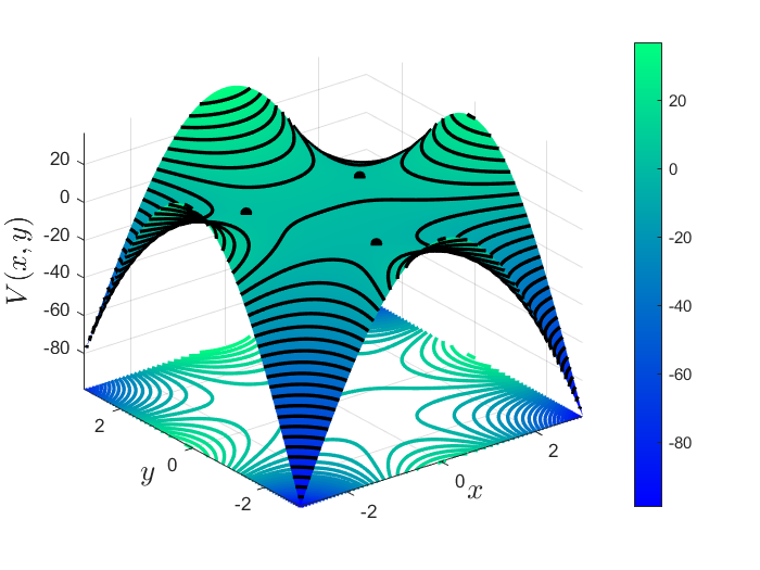
Figure 1: The 3D representation of the PES for $c_{1}=0.4,c_{2}=3,c_{3}=-0.3$

The dynamical significance of the index-1 saddles is that for energies above that of the saddles, there exist unstable periodic orbits (UPOs) in phase space. This is a consequence of the Lyapunov subcenter theorem Moser [1958]; Kelley [1967]. These UPOs, and their stable and unstable manifolds, are the essential phase space structures for understanding dynamical matching.

3 Phase Space Mechanism For the Existence and Non-existence of Dynamical Matching

We begin by explaining what we mean by dynamical matching in this potential energy surface with three index-1 saddles. In the ‘’usual” Caldera potential energy surfaces with two upper saddles and two lower saddles dynamical matching means that trajectories entering the Caldera region from the upper right saddle (resp. upper left saddle) move directly across the Caldera and exit by crossing the lower left saddle (resp. lower right saddle). For the Caldera potential energy surface with three index-1 saddles there is only a single lower index-1 saddle in the center of the lower regions. However, one can see from Fig. 1 that there is an exit region to the left (left exit region, LER) of the saddle and an exit region to the right (right exit region, RER) of the saddle. In this case, dynamical matching corresponds to trajectories that enter the Caldera from the upper right saddle (resp. upper left saddle), move directly across the Caldera, and exit from the LER (resp. RER).

Both the existence and non-existence of dynamical matching in this model can be explained by heteroclinic connections between the unstable manifolds of the upper UPOs and the stable manifold of the UPO associated with the lower saddle (lower UPO) and the geometry of the unstable manifold of the lower UPO.

We will study the geometry of these manifolds by using the method of Lagrangian descriptors (LDs), described in Appendix A. In order to study the manifolds near the upper saddles we apply the method of LDs in the 2D slice $y=0.84$ with $p_{y}>0$ (for a value of energy $E=2.821$) since this is the $y$-coordinate of the upper index-1 saddles (see the panels A and B of Fig. 2).

This the geometric structures on this slice reveal the unstable manifolds of the unstable periodic orbits of the upper index-1 saddles. We will focus on the right hand side of this slice (see panels C and D of Fig. 2) in order to study in detail the invariant manifolds that emanate from the unstable periodic orbits of the right upper index-1 saddle. In particular, we will describe the phase space mechanism for the case of the upper right index-1 saddle since for the case of the upper left saddle we have similar mechanism as a result of the symmetry of the potential.

Next we extract the invariant manifolds of the panels C and D of Fig. 2 using the gradient of LDs (see details in Katsanikas et al. [2020b]). We can see the result in Fig. 3. In this figure, we see many lobes between unstable and stable invariant manifolds. This is the unstable manifold of the UPO associated with the upper right saddle and the stable manifold associated the UPO of the lower saddle. We can verify this as follows. In the right corner of this figure we depict a position of a trajectory inside a lobe. If we integrate this trajectory backwards and forwards, the result will be the exit of this trajectory from the caldera through the region of the upper right index-1 saddle and the region of the lower right exit (see Fig. 4), respectively. This means that this lobe corresponds to a lobe between intersections of the unstable invariant manifold of the unstable periodic orbits of the UPO of the upper right index-1 saddle with the stable invariant manifold of the UPO family of the lower index-1 saddle (that is located at the center). The trajectories that are initially at the region of the right upper saddle follow the unstable invariant manifolds of the UPO associated with the right upper saddle until they are trapped in the lobes between the heteroclinic intersections of the unstable invariant manifolds of the right upper index-1 saddle with the stable invariant manifolds of the UPO of the lower index-1 saddle. Then the trajectories follow the stable invariant manifolds to the area of these unstable periodic orbits (the central area of the Caldera). This is the reason that the trajectory that corresponds to the black point of Fig. 3, moves towards the central area forward in time (as indicated from the arrows in Fig. 4). This explains the first part of the mechanism, the transport of the trajectories from the region of the upper index-1 saddle to the central area of the caldera.

The second part of the mechanism explains the transport of the trajectories from the area of the lower index-1 saddle (central area of the caldera) to one of the lower exits from the Caldera (for example the lower right exit from the Caldera for the trajectory of Fig. 4). In order to see this we use the method of LDs in the slice $y=0$ with $p_{y}>0$ to detect the invariant manifolds emanating from the central area of the caldera and, in particular, the invariant manifolds of the lower index-1 saddle. In Fig. 5, we depict, using LDs, the unstable and stable invariant manifolds of the central area. The next step is to extract the invariant manifolds of the panels A and B of Fig. 5 using the gradient of LDs (see details in Katsanikas et al. [2020b]). We can see the result in Fig. 6. In this Figure, we see the unstable and stable manifolds start from the point of the periodic orbit of the lower index-1 saddle (that is located at the center). The trajectories that approach the periodic orbit are on the stable manifolds (the motion of these trajectories is indicated by the violet arrows in Fig. 6). The trajectories that move away from the periodic orbit are on the unstable manifolds (the motion of these trajectories is indicated by the green arrows in Fig. 6. This means that the trajectories in the first part of the mechanism approach the neighborhood of the periodic orbit of the lower index-1 saddle (that is located in the central area of the caldera) will leave from this neighborhood following the unstable manifolds in one of the two directions that are indicated by the green arrows in Fig. 6. In each of these two directions, we take one initial condition (see the black points in Fig. 6) and we integrate it forward in time. In this way, we want to check the fate of the trajectories that will follow the one or the other direction of the unstable manifolds. When we integrate these initial conditions, we observe in the panel A of Fig. 7 that the trajectory that corresponds to the black point on the right side from the center (where the periodic orbit of the lower index-1 saddle is located) exits through the region of the lower right exit. On the contrary, when we integrate the other initial condition (the black point on the left side from the center of Fig. 6) the corresponding trajectory exits through the region of the lower left exit (see panel B of Fig. 7). We see that the two directions of the unstable manifolds that are emanated from the unstable periodic orbit of the lower index-1 saddle guide the trajectories directly to different exit regions. This means that the trajectories that are in the neighborhood of the unstable periodic orbits of the lower index-1 saddles in the central area of the caldera leave this area following the unstable invariant manifolds of these periodic orbits. If they follow the one direction of the unstable invariant manifolds exit through the one lower exit region and if they follow the other direction, they exit through the other lower exit region. This indicates the important role of the periodic orbits of the lower index-1 saddle that control through the direction of the unstable invariant manifolds the exit of the trajectories that come from the region of the upper index-1 saddles to the central area of the caldera.

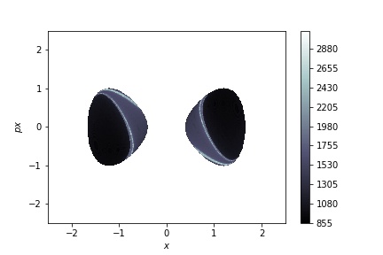
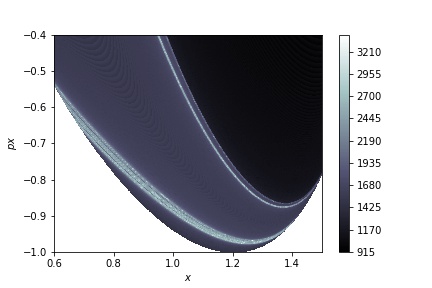
A) B)
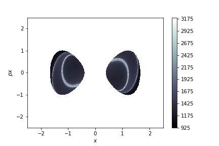
C) D)

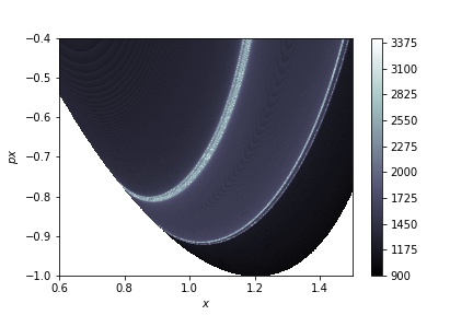
Figure 2: Computation of variable-time LDs in the 2D slide $y=0.84$ using $\tau=8$ and p = 1/2 for value of energy $E=2.821$. A) Forward integration LDs; B) Backward integration LDs; C) Forward integration for the interval $0.6<x<1.5$ and $-1<p_{x}<-0.4$ . D) Backward integration for the interval $0.6<x<1.5$ and $-1<p_{x}<-0.4$.

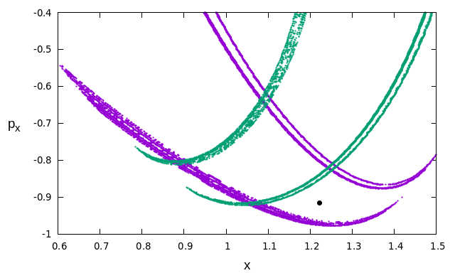
Figure 3: The stable (violet) and unstable (green) invariant manifolds extracted (in the 2D slice $y=0.84$ with $p_{y}>0$) from the gradient of the Lagrangian descriptors for the interval $0.6<x<1.5$ and $-1<p_{x}<-0.4$. We depict using black color the initial condition of a trajectory.

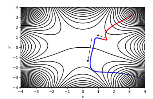
Figure 4: The contours of the Caldera potential and a trajectory in the configuration space forward (with blue color) and backward (with red color) in time (the initial condition of this trajectory is depicted by a black point in Fig. 3). The arrows denote the direction of the trajectory forward in time.

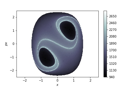
A) B)

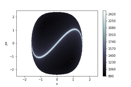
Figure 5: Computation of variable-time LDs in the 2D slice $y=0$ using $\tau=5$ and p = 1/2 for value of energy $E=2.821$. A) Forward integration LDs; B) Backward integration LDs;

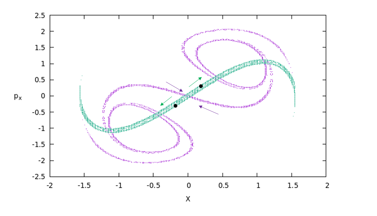
Figure 6: The stable (violet) and unstable (green) invariant manifolds extracted (in the 2D slice $y=0$ with $p_{y}>0$) from the gradient of the Lagrangian descriptors for the interval $-2.5<x<2.5$ and $-2.5<p_{x}<2.5$. We depict using black color the initial conditions of two trajectories on the unstable manifold. The green and violet arrows present the directions of the unstable and stable invariant manifolds respectively that are emanated from the unstable periodic orbit of the lower index-1, that is located at the center.

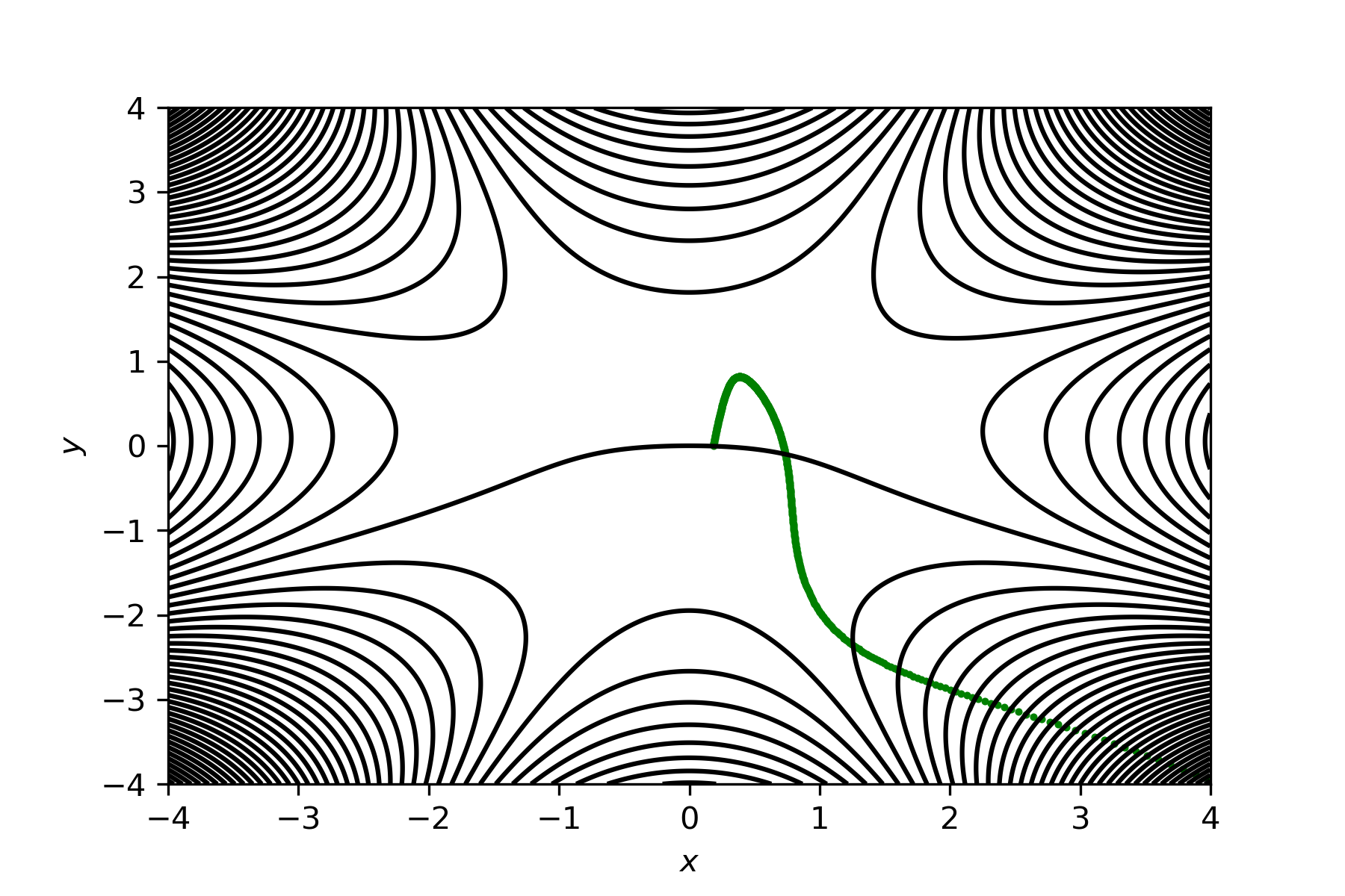
A) B)

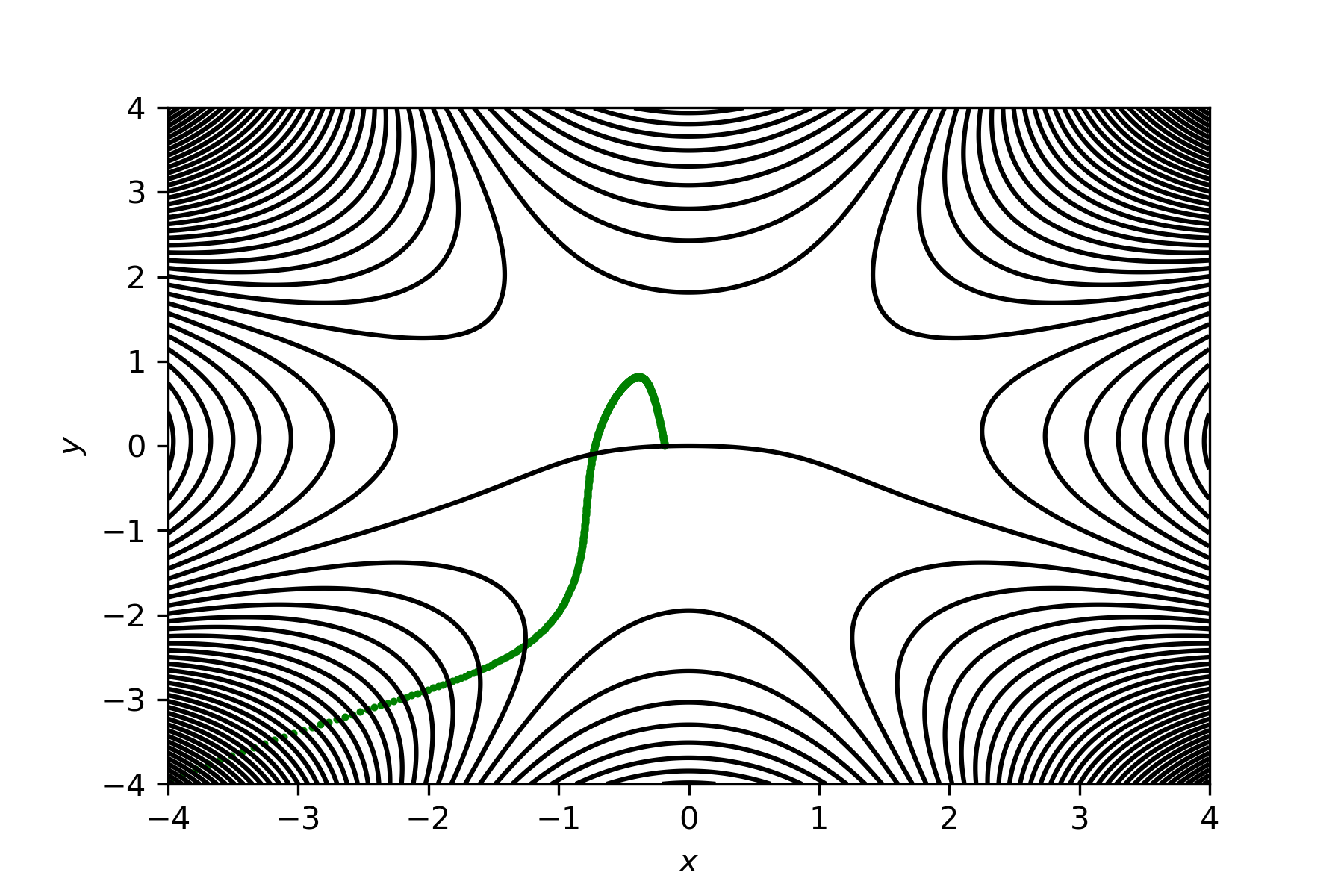
Figure 7: The contours of the caldera potential and two trajectories in the configuration space forward in time (with green color). The initial conditions of these trajectories correspond to the two black points in the right side from the center in Fig. 6 (for panel A) and in the left side from the center in Fig. 6 (for panel B).

4 Conclusions

In this paper, we investigated the phase space mechanism of transport that is responsible for the creating and breaking the phenomenon of dynamical matching (that was observed in Geng et al. [2021a, b]) for the form of a Caldera potential energy surface with only three index-1 saddles and no minimum. The first part of the mechanism is based on heteroclinic intersections of the unstable invariant manifolds of the unstable periodic orbits of the upper index-1 saddles and the stable invariant manifolds of the unstable periodic orbits of the lower index-1 saddle. This explains the transport from the region of the upper index-1 saddles to the region of the lower index-1 saddle. The second part of the mechanism is based on the direction of the unstable invariant manifolds of the unstable periodic orbits of the lower index-1 saddle. The trajectories leave the central area of the caldera following the unstable invariant manifolds of the unstable periodic orbits of the lower index-1 saddle. This happens in two directions. One direction guides the trajectories to the region of the lower left exit region and the other to the region of the lower right exit region. The unstable periodic orbits of the lower index-1 saddle control the transport from the central region of the caldera to the lower exit regions.

AcknowledgmentsThe authors acknowledge the financial support provided by the EPSRC Grant No. EP/P021123/1 and MA acknowledges support from the grant CEX2019-000904-S and IJC2019-040168-I funded by: MCIN/AEI/ 10.13039/501100011033.

5 appendix

The Lagrangian Descriptors is a diagnostic tool that can reveal the phase space structures. The first time that this technique was used was in the paper Madrid & Mancho [2009], were was aiming to study transport and mixing in geophysical flows. In the last years this technique has been broadly used not only in fluid mechanics Lopesino et al. [2015]; Balibrea-Iniesta et al. [2016]; Mendoza & Mancho [2010]; Mancho et al. [2013]; García-Garrido et al. [2018]; Balibrea-Iniesta et al. [2019]; Lopesino et al. [2017] but also in the area of chemical reaction dynamics Agaoglou et al. [2019, 2020, 2019]; Katsanikas et al. [2020a]; Crossley et al. [2021]. The LDs method works in the following way: In order to reveal the phase space structures in a given slice using the method of LDs the steps that we need to follow are very simple. First we choose the slice and we define in this slice a grid of initial conditions. Then we integrate this initial conditions forward and backward in time for a given integration time $\tau$ and while we are integrating we accumulate along these trajectories a positive quantity defined from the vector field that determines the dynamical system that we are studying. If you integrate trajectories forwards in time, the LD function is going to detect the stable manifolds while the backwards in time integration will detect the unstable manifolds. The scalar output obtained from the method will highlight the location of the invariant stable and unstable manifolds intersecting this slice, which are detected at points where the values of LDs display an abrupt change.

There are several definitions for the M function. In this work we are using the p-norm definition of the method that relies on variable time integration, where $p\in(0,1]$ (the reader can find more information about the application of variable time LDs to Caldera potentials in Katsanikas et al. [2020b]). We have fixed the value of p to be $p=1/2$. This definition of the M function is preferable here due to the nature of the Caldera’s potential energy surface (PES), that is an open potential. That can lead to an increasingly fast pace escape of the trajectories.

Let’s consider the following dynamical system with time dependence:

$$\dfrac{d\mathbf{x}}{dt}=\mathbf{v}(\mathbf{x},t)\;,\quad\mathbf{x}\in\mathbb{R}^{n}\;,\;t\in\mathbb{R}\;$$ (4)

where $\mathbf{v}(\mathbf{x},t)\in C^{r}(r\geq 1)$ in $\mathbf{x}$ and it is continuous in time. Given an initial condition $x_{0}$ at time $t_{0}$, take a fixed integration time $\tau>0$ and $p\in(0,1]$. The method of LDs in the p-norm definition is as follows:

$$M_{p}(\mathbf{x}_{0},t_{0},\tau)=\sum_{k=1}^{n}\bigg{[}\int^{t_{0}+\tau}_{t_{0}-\tau}|v_{k}(\mathbf{x}(t;\mathbf{x}_{0}),t)|^{p}\;dt\bigg{]}=M_{p}^{(b)}(\mathbf{x}_{0},t_{0},\tau)+M_{p}^{(f)}(\mathbf{x}_{0},t_{0},\tau)\;,$$ (5)

where $M_{p}^{(b)}$ and $M_{p}^{(f)}$ its backward and forward integration parts:

$$\begin{split}M_{p}^{(b)}(\mathbf{x}_{0},t_{0},\tau)&=\sum_{k=1}^{n}\bigg{[}\int^{t_{0}}_{t_{0}-\tau}|v_{k}(\mathbf{x}(t;\mathbf{x}_{0}),t)|^{p}\;dt\bigg{]}\;,\\[5.69046pt] M_{p}^{(f)}(\mathbf{x}_{0},t_{0},\tau)&=\sum_{k=1}^{n}\bigg{[}\int^{t_{0}+\tau}_{t_{0}}|v_{k}(\mathbf{x}(t;\mathbf{x}_{0}),t)|^{p}\;dt\bigg{]}\;,\end{split}$$ (6)

The formulation of the p-norm definition that we apply to this model is the following:

$$M_{p}(\mathbf{x}_{0},t_{0},\tau)=\sum_{k=1}^{n}\bigg{[}\int^{t_{0}+\tau_{x_{0}}^{+}}_{t_{0}-\tau_{x_{0}}^{-}}|v_{k}(\mathbf{x}(t;\mathbf{x}_{0}),t)|^{p}\;dt\bigg{]}$$ (7)

where

$$\tau_{x_{0}}^{\pm}=min\{\tau_{0},|t^{\pm}|_{|x(t^{\pm};x_{0}\notin R)}\}$$

Note that the integration time $\tau_{0}$ is fixed and that $t^{+}$ is the time that the trajectory exits the interaction region $R$ in forward time whereas $t^{-}$ is for backward time.

References

- Agaoglou et al. [2019] Agaoglou, M., Aguilar-Sanjuan, B., García-Garrido, V. J., García-Meseguer, R., González-Montoya, F., Katsanikas, M., Krajňák, V., Naik, S. & Wiggins, S. [2019] Chemical Reactions: A Journey into Phase Space (Bristol, UK, Zenodo), 10.5281/zenodo.3568210.
- Agaoglou et al. [2020] Agaoglou, M., Aguilar-Sanjuan, B., García-Garrido, V. J., González-Montoya, F., Katsanikas, M., Krajňák, V., Naik, S. & Wiggins, S. [2020] Lagrangian Descriptors: Discovery and Quantification of Phase Space Structure and Transport (zenodo: 10.5281/zenodo.3958985), 10.5281/zenodo.3958985.
- Athanassoula et al. [2009] Athanassoula, E., Romero-Gómez, M., Bosma, A. & Masdemont, J. [2009] “Rings and spirals in barred galaxies–ii. ring and spiral morphology,” Monthly Notices of the Royal Astronomical Society 400, 1706–1720.
- Balibrea-Iniesta et al. [2016] Balibrea-Iniesta, F., Lopesino, C., Wiggins, S. & Mancho, A. M. [2016] “Lagrangian descriptors for stochastic differential equations: A tool for revealing the phase portrait of stochastic dynamical systems,” International Journal of Bifurcation and Chaos 26, 1630036, 10.1142/S0218127416300366.
- Balibrea-Iniesta et al. [2019] Balibrea-Iniesta, F., Xie, J., García-Garrido, V. J., Bertino, L., Mancho, A. M. & Wiggins, S. [2019] “Lagrangian transport across the upper arctic waters in the canada basin,” Quarterly Journal of the Royal Meteorological Society 145, 76–91, 10.1002/qj.3404.
- Carpenter [1985] Carpenter, B. K. [1985] “Trajectories through an intermediate at a fourfold branch point. implications for the stereochemistry of biradical reactions,” Journal of the American Chemical Society 107, 5730–5732, 10.1021/ja00306a021.
- Collins et al. [2014] Collins, P., Kramer, Z., Carpenter, B., Ezra, G. & Wiggins, S. [2014] “Nonstatistical dynamics on the caldera,” Journal of Chemical Physics 141.
- Crossley et al. [2021] Crossley, R., Agaoglou, M., Katsanikas, M. & Wiggins, S. [2021] “From poincaré maps to lagrangian descriptors: The case of the valley ridge inflection point potential,” Regular and Chaotic Dynamics 26, 147–164.
- García-Garrido et al. [2018] García-Garrido, V. J., Curbelo, J., Mancho, A. M., Wiggins, S. & Mechoso, C. R. [2018] “The application of lagrangian descriptors to 3d vector fields,” Regul Chaotic Dyn 23, 551–568, 10.1134/S1560354718050052.
- Geng et al. [2021a] Geng, Y., Katsanikas, M., Agaoglou, M. & Wiggins, S. [2021a] “The bifurcations of the critical points and the role of the depth in a symmetric caldera potential energy surface,” Int. J. Bifurcation Chaos 31.
- Geng et al. [2021b] Geng, Y., Katsanikas, M., Agaoglou, M. & Wiggins, S. [2021b] “The influence of a pitchfork bifurcation of the critical points of a symmetric caldera potential energy surface on dynamical matching,” Chemical Physics Letters 768, 138397.
- Katsanikas et al. [2020a] Katsanikas, M., García-Garrido, V. J., Agaoglou, M. & Wiggins, S. [2020a] “Phase space analysis of the dynamics on a potential energy surface with an entrance channel and two potential wells,” Physical Review E 102, 012215.
- Katsanikas et al. [2020b] Katsanikas, M., García-Garrido, V. J. & Wiggins, S. [2020b] “Detection of dynamical matching in a caldera hamiltonian system using lagrangian descriptors,” Int. J. Bifurcation Chaos 30, 2030026.
- Katsanikas et al. [2020c] Katsanikas, M., García-Garrido, V. J. & Wiggins, S. [2020c] “The dynamical matching mechanism in phase space for caldera-type potential energy surfaces,” Chemical Physics Letters 743, 137199, https://doi.org/10.1016/j.cplett.2020.137199.
- Katsanikas & Wiggins [2018] Katsanikas, M. & Wiggins, S. [2018] “Phase space structure and transport in a caldera potential energy surface,” International Journal of Bifurcation and Chaos 28, 1830042.
- Katsanikas & Wiggins [2019] Katsanikas, M. & Wiggins, S. [2019] “Phase space analysis of the nonexistence of dynamical matching in a stretched caldera potential energy surface,” International Journal of Bifurcation and Chaos 29, 1950057.
- Katsanikas & Wiggins [2022] Katsanikas, M. & Wiggins, S. [2022] “The nature of reactive and non-reactive trajectories for a three dimensional caldera potential energy surface,” Physica D: Nonlinear Phenomena , 133293.
- Kelley [1967] Kelley, A. [1967] “On the Liapounov subcenter manifold,” Journal of mathematical analysis and applications 18, 472–478.
- Lopesino et al. [2017] Lopesino, C., Balibrea-Iniesta, F., García-Garrido, V. J., Wiggins, S. & Mancho, A. M. [2017] “A theoretical Framework for Lagrangian Descriptors,” Int J Bifurc Chaos 27, 1730001, 10.1142/S0218127417300014.
- Lopesino et al. [2015] Lopesino, C., Balibrea-Iniesta, F., Wiggins, S. & Mancho, A. M. [2015] “Lagrangian descriptors for two dimensional, area preserving, autonomous and nonautonomous maps,” Communications in Nonlinear Science and Numerical Simulation 27, 40–51, https://doi.org/10.1016/j.cnsns.2015.02.022.
- Madrid & Mancho [2009] Madrid, J. A. J. & Mancho, A. M. [2009] “Distinguished trajectories in time dependent vector fields,” Chaos 19, 013111, 10.1063/1.3056050.
- Mancho et al. [2013] Mancho, A. M., Wiggins, S., Curbelo, J. & Mendoza, C. [2013] “Lagrangian descriptors: A method for revealing phase space structures of general time dependent dynamical systems,” Commun. Nonlinear Sci. Numer. Simul. 18, 3530–3557, https://doi.org/10.1016/j.cnsns.2013.05.002.
- Mendoza & Mancho [2010] Mendoza, C. & Mancho, A. M. [2010] “The hidden geometry of ocean flows,” Phys. Rev. Lett. 105, 038501, https://journals.aps.org/prl/abstract/10.1103/PhysRevLett.105.038501.
- Moser [1958] Moser, J. [1958] “On the generalization of a theorem of A. Liapounoff,” Communications on Pure and Applied Mathematics 11, 257–271.