Similarity reductions of peakon equations: integrable cubic equations

Abstract

We consider the scaling similarity solutions of two integrable cubically nonlinear partial differential equations (PDEs) that admit peaked soliton (peakon) solutions, namely the modified Camassa-Holm (mCH) equation and Novikov’s equation. By making use of suitable reciprocal transformations, which map the mCH equation and Novikov’s equation to a negative mKdV flow and a negative Sawada-Kotera flow, respectively, we show that each of these scaling similarity reductions is related via a hodograph transformation to an equation of Painlevé type: for the mCH equation, its reduction is of second order and second degree, while for Novikov’s equation the reduction is a particular case of Painlevé V. Furthermore, we show that each of these two different Painlevé-type equations is related to the particular cases of Painlevé III that arise from analogous similarity reductions of the Camassa-Holm and the Degasperis-Procesi equation, respectively. For each of the cubically nonlinear PDEs considered, we also give explicit parametric forms of their periodic travelling wave solutions in terms of elliptic functions. We present some parametric plots of the latter, and, by using explicit algebraic solutions of Painlevé III, we do the same for some of the simplest examples of scaling similarity solutions, together with descriptions of their leading order asymptotic behaviour.

1 Introduction

1.1 Background and motivation

Painlevé transcendents can naturally be regarded as nonlinear analogues of the classical special functions. Classical special functions, such as Legendre polynomials, Hermite polynomials, or Bessel functions, which satisfy linear ordinary differential equations (ODEs), arise in the solution of linear partial differential equations (PDEs) by the method of separation of variables. In a similar way, Painlevé transcendents, which satisfy nonlinear ODEs, provide similarity solutions of soliton-bearing PDEs that are solvable by the inverse scattering transform [1, 16], and are now known to describe universal features of critical behaviour in such nonlinear PDEs (see e.g. [13]), as well as appearing in the treatment of scaling phenomena and other aspects of random matrices, statistical mechanics and quantum field theories (see [26] and chapter 32 in [36] for references to these and various other applications). The aim of this paper is to explain how, in a somewhat indirect way, Painlevé equations appear in the analysis of scaling similarity reductions of certain integrable nonlinear PDEs that admit peaked soliton solutions (peakons).

The cubically nonlinear PDE given by

$$u_{t}-u_{xxt}+3u^{2}u_{x}+2u_{x}u_{xx}^{2}+u_{x}^{2}u_{xxx}=u_{x}^{3}+4uu_{x}u_{xx}+u^{2}u_{xxx}$$ (1.1)

is commonly known as the modified Camassa-Holm (mCH) equation (see e.g. [23], or [10, 41]), because it is related via a reciprocal transformation to a negative flow in the modified KdV hierarchy, while the Camassa-Holm equation [5], that is

$$u_{t}-u_{xxt}+3uu_{x}=2u_{x}u_{xx}+uu_{xxx},$$ (1.2)

has an analogous relationship with a corresponding negative flow in the KdV hierarchy. These and similar equations arise as truncations of asymptotic series approximations in shallow water theory [6, 9, 14, 15, 29], as bi-Hamiltonian equations admitting infinitely many commuting symmetries generated by a recursion operator [17, 32, 35], and as compatibility conditions coming from a Lax pair [18, 38]. In these various contexts, the equation (1.2) can appear with additional linear dispersion ($u_{x}$ and $u_{xxx}$) terms, while (1.1) can have suitable linear and quadratic nonlinear terms included, but such terms can always be removed by a combination of a Galilean transformation and a shift $u\to u+\,$const, which changes the boundary conditions. However, such transformations are irrelevant from the point of view of integrability, which is determined by the underlying algebraic structure of the equations and their symmetries, so here we will always work with the pure dispersionless versions of these equations.

Aside from their connections with shallow water models and bi-Hamiltonian theory, perhaps the most remarkable feature of the dispersionless forms of these equations, as discovered in [5] for (1.2), is the fact that they admit weak solutions in the form of peaked solitons with discontinuous derivatives at the peaks, given by

$$u(x,t)=\sum_{j=1}^{N}p_{j}(t)\exp\big{(}-|x-q_{j}(t)|\big{)},$$ (1.3)

where $q_{j}(t)$ are the positions of the peaks and $p_{j}(t)$ are the amplitudes, which satisfy a finite-dimensional Hamiltonian system of ODEs. Due to this feature, we refer to these PDEs as peakon equations. The characteristic shape of the peakons can be understood by introducing the momentum density $m$, given by the 1D Helmholtz operator acting on the velocity field $u$, that is

$$m=(1-D_{x}^{2})u.$$ (1.4)

The introduction of $m$ allows the dispersionless versions of the PDEs to be rewritten in a very compact form: the Camassa-Holm equation (1.2) is equivalent to

$$m_{t}+um_{x}+2u_{x}m=0,$$ (1.5)

while the modified equation (1.1) is rewritten in the simple form

$$m_{t}+\big{(}m(u^{2}-u_{x}^{2})\big{)}_{x}=0.$$ (1.6)

Then since $\tfrac{1}{2}e^{-|x|}$ is the Green’s function for the Helmholtz operator, the momentum density (1.4) for the peakon solutions (1.3) is a sum of Dirac delta functions with support at the peak positions $q_{j}(t)$, $j=1,\ldots,N$. For more details of peakons and their connections with approximation theory, see the recent review [31] and references therein.

The other cubically nonlinear PDE we will be concerned with here is the equation

$$u_{t}-u_{xxt}+4u^{2}u_{x}=u^{2}u_{xxx}+3uu_{x}u_{xx},$$ (1.7)

which was found by Novikov in a classification of quadratic/cubic peakon-type equations admitting infinitely many symmetries [33]. Novikov’s equation can be written more concisely as

$$m_{t}+u^{2}m_{x}+3uu_{x}m=0,$$ (1.8)

with the same momentum variable as in (1.4). As shown in [28], it is related by a reciprocal transformation to a negative flow in the Sawada-Kotera hierarchy; so its relationship with the Degasperis-Procesi equation [12]

$$m_{t}+um_{x}+3u_{x}m=0,$$ (1.9)

which has a reciprocal transformation to a negative Kaup-Kupershmidt flow [11], is somewhat similar to the relationship between (1.1) and (1.2), because the Sawada-Kotera and Kaup-Kupershmidt hierarchies are related to the same modified hierarchy (see [19, 21] and references).

In this paper we are concerned with scaling similarity solutions of the cubic peakon equations (1.1) and (1.7). It is a surprising feature of all the peakon equations described so far that, despite being fundamentally nonlinear, they admit separable solutions of the form

$$u(x,t)=Y(t)U(x),$$

which are typically only a feature of linear PDEs. It turns out that (up to the trivial freedom to shift $t$ by a constant, which henceforth we will ignore) the function $Y$ is just a power of $t$, corresponding to a simple symmetry of each of these equations under scaling $u$ and $t$. For the cubic peakon equations being considered here, the separable solutions take the form

$$u(x,t)=t^{-1/2}U(x),$$ (1.10)

while for the quadratically nonlinear equations (1.2) and (1.9) these solutions have the form

$$u(x,t)=t^{-1}U(x)$$ (1.11)

instead.

Solutions of the form (1.11) for the Camassa-Holm equation (1.2) were discussed in [20], where it was shown that the ODE satisfied by $U(x)$ fails the Painlevé test. From this point of view, it would appear that such solutions are a counterexample to an assertion of Ablowitz, Ramani and Segur [1], which says that all ODEs obtained from similarity reductions of PDEs that are integrable (in the sense of admitting a Lax pair, so that they can be solved by the inverse scattering method) should be free of movable critical points. However, it has long been known that this assertion cannot be true in its most naive form, and the Camassa-Holm equation is a case in point: the expansion of the solutions of the PDE (1.2) itself in the neighbourhood of a movable singularity manifold displays algebraic branching [26], and this movable branching is inherited by the ODEs obtained from it via a similarity reduction, such as the equation for $U(x)$. Nevertheless, the solutions (1.11) belong to a one-parameter family of similarity reductions, found in [25], which can be solved in terms of certain Painlevé III transcendents, meaning that the assertion of [1] can be salvaged in this case. Although this would appear to contradict the result of [20], there is in fact no contradiction: the Painlevé property, and more specifically the third Painlevé equation

$$\frac{\mathrm{d}^{2}w}{\mathrm{d}{\zeta}^{2}}=\frac{1}{w}\left(\frac{\mathrm{d}w}{\mathrm{d}{\zeta}}\right)^{2}-\frac{1}{{\zeta}}\left(\frac{\mathrm{d}w}{\mathrm{d}{\zeta}}\right)+\frac{1}{{\zeta}}\big{(}\tilde{{\alpha}}w^{2}+\tilde{{\beta}}\big{)}+\tilde{{\gamma}}w^{3}+\frac{\tilde{\delta}}{w}$$ (1.12)

(for some particular values of the parameters $\tilde{{\alpha}},\tilde{{\beta}},\tilde{{\gamma}},\tilde{\delta}$), only appears after making certain precise changes of the dependent and independent variables, including a hodograph-type transformation, which completely changes the singularity structure. Thus movable poles of $w$ in the complex ${\zeta}$ plane arise from movable algebraic branch points in terms of the original variables, i.e. $U$ and $x$ in (1.11).

In recent work [3], we studied similarity reductions of the so-called $b$-family of equations, given by

$$m_{t}+um_{x}+bu_{x}m=0,\qquad m=u-u_{xx},$$ (1.13)

with a constant coefficient $b$. It is known that the cases $b=2,3$, namely (1.2) and (1.9), are the only members of this family that are integrable in the sense of admitting infinitely many commuting local symmetries [32], and the only cases for which the prolongation algebra method provides a Lax pair of zero curvature type [27]. For any $b$, the equation (1.13) admits a one-parameter family of scaling similarity reductions which includes the separable solutions (1.11), and in particular the ramp profile

$$u(x,t)=\frac{x}{(b+1)t}$$ (1.14)

for $b\neq-1$. Beginning with [24], Holm and Staley did extensive studies on numerical solutions of (1.13), and revealed bifurcation phenomena controlled by the parameter $b$. Their results included numerically stable “ramp-cliff” solutions for $-1<b<1$, looking like the ramp (1.14) in a compact region, joined to a rapidly decaying cliff. The results in [3] show that the scaling similarity reductions of (1.13) are related via a transformation of hodograph type to a non-autonomous ODE of second order; but this ODE only has the Painlevé property in the integrable cases $b=2,3$, when it is equivalent to two different versions of the Painlevé III equation (1.12): the reduction already found for the Camassa-Holm equation in [25], and another set of values of $\tilde{{\alpha}},\tilde{{\beta}},\tilde{{\gamma}},\tilde{\delta}$ for the reduction of the Degasperis-Procesi equation.

1.2 Outline of the paper

An outline of the rest of the paper is as follows.

The next section is devoted to similarity reductions of the mCH equation (1.1). We begin by briefly reviewing the link between the Camassa-Holm equation and the first negative KdV flow via a reciprocal transformation, as well as the reciprocal transformation between (1.1) and the first negative mKdV flow, before presenting a precise formulation of the Miura map between these two negative flows (Proposition 2.1). Our main goal is then to describe the scaling similarity solutions of (1.1), but to pave the way towards this it is helpful to consider the travelling wave solutions beforehand. The latter are related to corresponding travelling waves of the first negative mKdV flow via a transformation of hodograph type, which is obtained by applying the travelling wave reduction to the reciprocal transformation. By reduction of the associated Miura map, these solutions are then connected to explicit elliptic function formulae for the travelling waves of the negative KdV equation, as found in [25]. This leads to an exact parametric solution for the smooth travelling waves of (1.1), in terms of Weierstrass functions, given in Theorem 2.2 below, and illustrated with plots of a particular solution (see Example 2.3). The same template is followed for the scaling similarity solutions of (1.1): the similarity reduction of the reciprocal transformation provides a hodograph-type link between these solutions and a Painlevé-type ODE of second order and second degree for corresponding solutions of the first negative mKdV equation; and the reduction of the Miura map gives a one-to-one correspondence between the second degree equation and the particular case of Painlevé III that is associated with the scaling similarity solutions of the negative KdV flow (Lemma 2.4). The main result of the section is the parametric form of the scaling similarity solutions of (1.1), given in terms of a solution of the second degree equation and a pair of tau functions for Painlevé III (Theorem 2.6). An explicit illustration of this result, together with the leading order asymptotics of two real branches in a particular similarity solution, is provided in Example 2.7, which is based on a simple algebraic solution of Painlevé III.

Section 3 is concerned with similarity reductions of Novikov’s equation (1.7). Initially, we review the two different Miura maps that relate the Kaup-Kupershmidt hierarchy and the Sawada-Kotera hierarchy to the same modified hierarchy, as well as the negative flows in each of these hierarchies which are linked via a reciprocal transformation to the Degasperis-Procesi equation (1.9), and to Novikov’s equation, respectively. Once again, to lay the groundwork for the subsequent results on scaling similarity solutions, it is helpful to first make a detailed analysis of the travelling waves for (1.7). By reduction of the reciprocal transformation connecting it to the negative Sawada-Kotera equation, these are related to the travelling wave solutions of the latter, which are given explicitly in terms of elliptic functions; hence the exact parametric form of the smooth travelling waves in Novikov’s equation is derived (Theorem 3.2), and a particular numerical example is plotted (Example 3.3). The analysis of the scaling similarity solutions follows a similar pattern: in this case, the reciprocal transformation reduces to a hodograph link with the solutions of a non-autonomous ODE of second order, which describes the corresponding scaling similarity reduction of the negative Sawada-Kotera flow. After a simple change of variables, this ODE is shown to be equivalent to a case of the fifth Painlevé equation, that is

$$\frac{\mathrm{d}^{2}w}{\mathrm{d}{\zeta}^{2}}=\left(\frac{1}{2w}+\frac{1}{w-1}\right)\left(\frac{\mathrm{d}w}{\mathrm{d}{\zeta}}\right)^{2}-\frac{1}{{\zeta}}\left(\frac{\mathrm{d}w}{\mathrm{d}{\zeta}}\right)+\frac{(w-1)^{2}}{{\zeta}^{2}}\Big{(}\tilde{{\alpha}}w+\frac{\tilde{{\beta}}}{w}\Big{)}+\frac{\tilde{{\gamma}}w}{{\zeta}}+\frac{\tilde{\delta}w(w+1)}{w-1},$$ (1.15)

with a particular restriction on the parameters, including the requirement that $\tilde{\delta}=0$. By a result due to Gromak [22], when this requirement holds, the Painlevé V equation (1.15) is solved with Painlevé III transcendents, and we use this to give a one-to-one correspondence between the ODEs for the scaling similarity solutions of the negative Sawada-Kotera and Kaup-Kupershmidt flows (Proposition 3.7). These ODEs have Bäcklund transformations, which can be deduced from the action of certain discrete symmetries that are inherited from the Miura maps for the two PDE hierarchies (see Corollary 3.8). The general scaling similarity solution of Novikov’s equation is then given parametrically in terms of a solution of the aforementioned ODE that is equivalent to a case of Painlevé V, together with two different tau functions related by a Bäcklund transformation (Theorem 3.9). As in the case of the reductions of the mCH equation, an illustration of the latter result is provided by starting from an elementary algebraic solution of Painlevé III (Example 3.10), for which we plot the corresponding scaling similarity solution of (1.7), and determine its leading order asymptotics for large positive/negative real values of the independent variable. To conclude the section, we consider the special case of the separable solutions of the form (1.10) in Novikov’s equation, which turn out to be given parametrically in terms of two different quadratures involving Bessel functions of order zero (Theorem 3.11).

The fourth and final section of the paper contains our conclusions.

Preliminary versions of some of these results on scaling similarity reductions of cubic peakon equations were presented in the thesis [2].

2 Reductions of the mCH equation

In this section, we consider reductions of the modified Camassa-Holm (mCH) equation (1.1). To begin with, we explain why the latter nomenclature is appropriate, by describing the relationship with the Camassa-Holm equation (1.2), which becomes apparent when suitable reciprocal transformations are applied to these two equations. In order to clearly distinguish between the two equations, we start from the Camassa-Holm equation in the form (1.5), and write the associated conservation law for the field $p=\sqrt{m}$, while at the same time replacing the other dependent/independent variables $u,x,t$ by $\bar{u},\bar{x},\bar{t}$, so that it becomes the system

$$\frac{\partial p}{\partial\bar{t}}+\frac{\partial}{\partial\bar{x}}(\bar{u}p)=0,\qquad p^{2}=(1-D_{\bar{x}}^{2})\bar{u}.$$ (2.1)

Henceforth in this section we reserve $m,u,x,t$ for the corresponding dependent/independent variables in the modified equation (1.6).

2.1 Miura map between negative flows

The first equation in (2.1) is a conservation law for the Camassa-Holm equation, which leads to the introduction of new independent variables $X,T$ via the reciprocal transformation

$$\mathrm{d}X=p\,\mathrm{d}\bar{x}-\bar{u}p\,\mathrm{d}\bar{t},\qquad\mathrm{d}T=\mathrm{d}\bar{t}.$$ (2.2)

By applying a reciprocal transformation to a PDE system, any conservation law in the original independent variables is transformed to another conservation law in terms of the new variables. For the Camassa-Holm equation, the result of applying the reciprocal transformation (2.2) is a PDE of third order for $p=p(X,T)$, which can be written in conservation form as

$$\frac{\partial}{\partial T}(p^{-1})+\frac{\partial}{\partial X}\big{(}p(\log p)_{XT}-p^{2}\big{)}=0.$$ (2.3)

(Here and throughout the rest of the paper, we abuse notation by using the same letter to denote a field variable as a function of both old and new independent variables, so $p(x,t)\to p(X,T)$.) An alternative way to express the equation (2.3) in conservation form, which makes the connection with the KdV hierarchy apparent, is

$$\frac{\partial V}{\partial T}+\frac{\partial p}{\partial X}=0,$$ (2.4)

where the quantity $V$ is defined in terms of $p$ by

$$pp_{XX}-\tfrac{1}{2}p_{X}^{2}+2Vp^{2}+\tfrac{1}{2}=0.$$ (2.5)

The quantity $V$ is the usual KdV field variable, which (up to scale) appears in the Lax pair as the potential in a Schrödinger operator, and it follows from (2.4) and (2.5) that ${\cal R}V_{T}=0$, where ${\cal R}=D_{X}^{2}+4V+2V_{X}D_{X}^{-1}$ is the recursion operator for the KdV hierarchy. Hence the PDE (2.3) obtained by applying the above reciprocal transformation to the Camassa-Holm equation corresponds to the first negative KdV flow (see [27] and references therein for further discussion).

An analogous reciprocal transformation for the modified equation (1.6) is defined by

$$\mathrm{d}X=\tfrac{1}{2}m\,\mathrm{d}x-\tfrac{1}{2}fm\,\mathrm{d}t,\qquad\mathrm{d}T=4\,\mathrm{d}t,$$ (2.6)

with

$$f=u^{2}-u_{x}^{2}.$$ (2.7)

The latter transformation (with $T$ rescaled) was presented in [28], where the connection with the modified KdV (mKdV) hierarchy was obtained by deriving the standard Miura map formula from the reciprocal transformation applied to the mCH Lax pair in the form given by Qiao [38]. Here we make this connection more explicit, and we shall see that the choice of scale factor 4 in the definition of $T$ is important in what follows.

Direct application of the transformation (2.6) to the modified Camassa-Holm equation (1.6) results in the conservation law

$$v_{T}=\tfrac{1}{8}f_{X},$$ (2.8)

where it is convenient to introduce the field

$$v=m^{-1}.$$ (2.9)

In order to obtain a single PDE for $v=v(X,T)$, it is necessary to make use of the definitions (2.7) and (1.4). These yield

$$f_{x}=2u_{x}m\implies vf_{X}=2u_{X}$$ (2.10)

and

$$m=u-u_{xx}\implies v^{-1}=u-\tfrac{1}{4}\big{(}v^{-1}D_{X}\big{)}^{2}u=u-\tfrac{1}{8}v^{-1}D_{X}(f_{X})=u-v^{-1}v_{XT},$$

where (2.8) was used to obtain the last equality, which rearranges to produce

$$u=v^{-1}(v_{XT}+1).$$ (2.11)

Then from (2.10) and (2.8) we have another conservation law, that is

$$\frac{\partial}{\partial T}(v^{2})=\tfrac{1}{2}u_{X},$$ (2.12)

and by substituting for $u$ from (2.11) in the right-hand side above, this gives a PDE of third order for $v$, namely

$$\frac{\partial}{\partial X}\Big{(}v^{-1}(v_{XT}+1)\Big{)}=4vv_{T}.$$ (2.13)

The equation (2.13) was not explicitly given in [28], where the result of the reciprocal transformation applied to (1.6) was instead written as a system, while the interpretation of this as a negative mKdV flow was inferred from the transformation of the Lax pair, revealing that the KdV field $V$ in (2.4) is given in terms of $v$ by the standard Miura relation

$$V=v_{X}-v^{2}.$$ (2.14)

We now describe the relation between (2.3) and (2.13) more precisely.

Proposition 2.1.

The first negative mKdV flow, given by (2.13), is mapped to the first negative KdV flow (2.3) by the Miura transformation

$$p=\tfrac{1}{2}v^{-1}(v_{XT}+1)-v_{T},$$ (2.15)

which has the Miura map (2.14) for the KdV field $V$ as a consequence. Conversely, if $p=p(X,T)$ is a solution of the PDE (2.3), then $v=v(X,T)$ defined by

$$v=-\tfrac{1}{2}p^{-1}(p_{X}-1),$$ (2.16)

satisfies the PDE (2.13).

• Using (2.11), the formula (2.15) can be rewritten as

  $$p=\tfrac{1}{2}u-v_{T},$$

  so if $v=v(X,T)$ is a solution of the equation (2.13) then

  $$p_{X}=\tfrac{1}{2}u_{X}-v_{XT}=2vv_{T}-v_{XT},$$ (2.17)

  by (2.12). Then upon rearranging (2.15), we find

  $$2vp-1=v_{XT}-2vv_{T},$$ (2.18)

  which means that applying the identity (2.17) yields

  $$2vp-1=-p_{X},$$

  and hence $v$ can be written in terms of $p$, in the form (2.16). This expression for $v$ then gives

  $$\begin{array}[]{rcl}v_{X}-v^{2}&=&\tfrac{\partial}{\partial X}\big{(}-\genfrac{}{}{}{2}{1}{2}p^{-1}(p_{X}-1)\big{)}-\genfrac{}{}{}{2}{1}{4}p^{-2}(p_{X}-1)^{2}\\ &=&-\genfrac{}{}{}{2}{1}{2}p^{-1}p_{XX}+\genfrac{}{}{}{2}{1}{4}p^{-2}(p_{X}^{2}-1),\end{array}$$ (2.19)

  where the expression on the last line is the definition of the KdV field $V$ in terms of $p$, according to (2.5); thus $V$ is given in terms of $v$ by the standard Miura formula (2.14). Differentiating the latter formula with respect to $T$ produces

  $$V_{T}=v_{XT}-2vv_{T},$$ (2.20)

  which implies $V_{T}=-p_{X}$, by using (2.17) once more. Thus $p=p(X,T)$ defined by (2.15) satisfies (2.4), which is equivalent to the PDE (2.3). For the converse, if $v$ is given in terms of a solution of (2.3) by (2.16), then the calculation (2.19) giving the Miura formula for $V$ in terms of $v$ holds, and its $T$ derivative yields the equality (2.20). Hence, by applying (2.3), $v_{XT}-2vv_{T}=-p_{X}$, or equivalently

  $$p_{X}+v_{XT}=2vv_{T},$$ (2.21)

  and then from (2.16) this implies that (2.18) holds, which in turn means that $p$ can be written in terms of $v$ according to (2.15). Finally, differentiating both sides of (2.15) with respect to $X$ and using this to substitute for $p_{X}$ in (2.21), the PDE (2.13) for $v$ follows. ∎

The preceding result shows exactly why “modified Camassa-Holm equation” is a suitable name for (1.6), since under a reciprocal transformation it is connected to (1.5) by a Miura map.

2.2 Travelling waves

Before treating the scaling similarity solutions, we first consider travelling waves of the mCH equation (1.6), setting

$$u(x,t)=U(z),\qquad m(x,t)=M(z),\qquad z=x-ct,$$ (2.22)

where $c$ is the wave velocity, and we will also write $F(z)$ for the quantity $U^{2}-U_{z}^{2}$ obtained from (2.7). As it is already in the form of a conservation law, (1.6) becomes a total $z$ derivative, so integrating this we obtain

$$(F-c)M+k=0,$$ (2.23)

where $k$ is an integration constant. Henceforth we will assume that $k\neq 0$, since if we are considering smooth solutions, then the case $k=0$ implies that either $F=c$, or $M=0$, both of which lead to unbounded solutions given in terms of exponential/hyperbolic functions; but the 1-peakon solution with $M$ being given by a delta function can be viewed as a weak limit of strong (analytic) solutions with $k=0$ [30]. In terms of $z$ derivatives, the first equality in (2.10) implies $M=\tfrac{1}{2}F_{z}/U_{z}$, which means that (2.23) integrates to yield

$$\tfrac{1}{4}(F-c)^{2}+kU=\ell,$$

for another integration constant $\ell$, which corresponds to an ODE of first order for $U(z)$, namely

$$U_{z}^{2}-U^{2}\pm 2\sqrt{\ell-kU}+c=0.$$ (2.24)

The latter equation is easily reduced to a quadrature, but a more useful approach is to employ the reciprocal transformation (2.6), which leads to an explicit parametric form for the general solution.

If we take the reciprocally transformed equation (2.8), written in the form

$$(m^{-1})_{T}=\tfrac{1}{8}f_{X},$$

then reducing to travelling waves with velocity $\tilde{c}$ we have dependent variables $U(Z)$, $M(Z)$, $F(Z)$, considered as functions of

$$Z=X-\tilde{c}T,$$ (2.25)

and the conservation law (2.8) reduces to a total $Z$ derivative, which integrates to give

$$-\tilde{c}M^{-1}=\tfrac{1}{8}F+\mathrm{const}.$$

The above equation is equivalent to (2.23) if we identify the integration constant with $-\tfrac{1}{8}c$, and $k=8\tilde{c}\neq 0$, so that

$$M(F-c)+8\tilde{c}=0,$$ (2.26)

Thus we see that the travelling wave reduction of the mCH equation (1.6) corresponds to the travelling wave reduction of the PDE (i.e., the first negative mKdV flow) that is obtained from it via the reciprocal transformation (2.6), provided that the parameters $c,\tilde{c}$ are appropriately identified as velocities/integration constants, with their roles interchanged in passing between the two equations. Furthermore, it turns out that (2.6) reduces to a hodograph transformation between the ODEs obtained from these reductions, since

$$\begin{array}[]{rcl}\mathrm{d}Z&=&\mathrm{d}X-\tilde{c}\,\mathrm{d}T\\ &=&\genfrac{}{}{}{2}{1}{2}m\,\mathrm{d}x-\genfrac{}{}{}{2}{1}{2}fm\,\mathrm{d}t-4\tilde{c}\,\mathrm{d}t\\ &=&\genfrac{}{}{}{2}{1}{2}M\,\mathrm{d}x-\genfrac{}{}{}{2}{1}{2}MF\,\mathrm{d}t+\genfrac{}{}{}{2}{1}{2}M(F-c)\,\mathrm{d}t\\ &=&\genfrac{}{}{}{2}{1}{2}M\,(\mathrm{d}x-c\,\mathrm{d}t)\\ &=&\genfrac{}{}{}{2}{1}{2}M\,\mathrm{d}z.\end{array}$$ (2.27)

There are two ways to make use of the equation (2.26), viewed as the travelling wave reduction of the reciprocally transformed conservation law (2.8). First of all, the reductions of (2.10) and (1.4), transformed into expressions involving $Z$ derivatives, give

$$F_{Z}=2MU_{Z},$$ (2.28)

and

$$M=U-\tfrac{1}{4}M\frac{\mathrm{d}}{\mathrm{d}Z}(MU_{Z}),$$

while (2.7) becomes

$$F=U^{2}-\tfrac{1}{4}(MU_{Z})^{2}.$$

Using (2.28) to eliminate $U_{Z}$ from the latter two equations, we find that

$$U=M\big{(}\tfrac{1}{8}F_{ZZ}+1\big{)}=-\frac{8\tilde{c}}{F-c}\left(\frac{1}{8}F_{ZZ}+1\right),$$ (2.29)

where (2.26) was used to obtain the last equality, by substituting for $M$, and also

$$U^{2}=\tfrac{1}{16}F_{Z}^{2}+F.$$ (2.30)

Upon comparing the two expressions (2.29) and (2.30) for $U$, an ODE of second order and second degree for $F=F(Z)$ results, namely

$$\frac{64\tilde{c}^{2}}{(F-c)^{2}}\big{(}\tfrac{1}{8}F_{ZZ}+1\big{)}^{2}=\tfrac{1}{16}F_{Z}^{2}+F.$$ (2.31)

However, a second way to view this reduction is to consider the quantity $\tilde{v}(Z)$ obtained by reducing $v(X,T)$ to a travelling wave, so that

$$\tilde{v}(Z)=\frac{1}{M(Z)}=\frac{c-F(Z)}{8\tilde{c}}.$$ (2.32)

Applying the travelling wave reduction directly to the PDE (2.13), it is clear that each side is a total $Z$ derivative, so upon integrating and rearranging, an ODE of second order for $\tilde{v}$ arises, that is

$$\tilde{c}\frac{\mathrm{d}^{2}\tilde{v}}{\mathrm{d}Z^{2}}-2\tilde{c}\tilde{v}^{3}+\tilde{k}\tilde{v}-1=0,$$ (2.33)

where $\tilde{k}$ is an integration constant.

The equation (2.33) is solved in terms of elliptic functions. A shortcut to deriving the explicit form of these solutions is provided by Proposition 2.1: there is a Miura map between the solutions of (2.33) and the travelling wave solutions of (2.3), as presented in [3] (see also [25]). Identifying $\tilde{c}$ with the wave velocity $d$ in [3], the travelling waves of (2.3) correspond to a KdV field $V(Z)=-2\wp(Z)-\wp(W)$ (up to the freedom to replace $Z\to Z+\,$const), where $W$ is an arbitrary constant, so that the Miura formula (2.14) requires that

$$\frac{\mathrm{d}\tilde{v}}{\mathrm{d}Z}-\tilde{v}^{2}=-2\wp(Z)-\wp(W).$$ (2.34)

This implies that $\tilde{v}=-\tfrac{\mathrm{d}}{\mathrm{d}Z}\log\psi$, where $\psi$ satisfies the Schrödinger equation

$$\frac{\mathrm{d}^{2}\psi}{\mathrm{d}Z^{2}}-2\wp(Z)\psi=\wp(W)\psi,$$ (2.35)

equivalent to the simplest case of Lamé’s equation. A direct calculation then shows that taking

$$\psi(Z)=\frac{{\sigma}(Z+W)}{{\sigma}(Z)}\exp\big{(}-{\zeta}(W)Z\big{)},$$ (2.36)

with ${\sigma}$ and $\zeta$ denoting the Weierstrass sigma and zeta functions, respectively, gives the general solution of (2.33) in the form

$$\tilde{v}(Z)=-\frac{1}{2}\left(\frac{\wp^{\prime}(Z)-\wp^{\prime}(W)}{\wp(Z)-\wp(W)}\right),$$ (2.37)

up to the freedom to shift $Z\to Z-Z_{0}$, for an arbitrary constant $Z_{0}$ (since the ODE for $\tilde{v}$ is autonomous), provided that the parameters are given by

$$\tilde{c}=-\frac{1}{2\wp^{\prime}(W)},\qquad\tilde{k}=6\tilde{c}\wp(W).$$ (2.38)

The solution (2.37) can also be obtained more directly from the travelling wave reduction of (2.3), which is given by $p(X,T)=P(Z)$ with

$$P(Z)=\frac{\wp(Z)-\wp(W)}{\wp^{\prime}(W)}$$

(cf. equation (2.14) in [3]), by applying this reduction to the formula (2.16). This gives

$$\tilde{v}=-\frac{\Big{(}\tfrac{\mathrm{d}P}{\mathrm{d}Z}-1\Big{)}}{2P},$$

and then substituting the explicit form of $P$ as above yields the required expression for $\tilde{v}$. Observe that the resulting solution (2.37) depends on three parameters, namely $W$ and the invariants $g_{2},g_{3}$ of the Weierstrass $\wp$ function, so together with the arbitrary shift $Z_{0}$ this makes a total of four free parameters, corresponding to the two coefficients $\tilde{c},\tilde{k}$ plus two initial data required to specify the initial value problem for (2.33).

The relation (2.32) shows that the solution of the second degree equation (2.31) for $F$ should be given by

$$F(Z)=c-8\tilde{c}\tilde{v}(Z),$$ (2.39)

with $\tilde{v}$ specified according to (2.37), and a direct calculation shows that indeed this is the case, provided that the parameter $c$ is taken as

$$c=\frac{2\wp^{\prime\prime}(W)}{\wp^{\prime}(W)^{2}}.$$ (2.40)

Finally, comparing (2.29) with (2.39) and (2.33), we find that the quantity $U$ can be expressed in terms of $\tilde{v}$ as

$$U(Z)=-2\tilde{c}\tilde{v}(Z)^{2}+\tilde{k}.$$ (2.41)

This allows the travelling wave solutions of the mCH equation to be expressed in parametric form.

Theorem 2.2.

The smooth travelling wave solutions (2.22) of the mCH equation (1.1) are given parametrically by $U=U(Z)$, $z=z(Z)$, where $U(Z)$ is defined by (2.41) with $\tilde{v}(Z)$ as in (2.37) (up to the freedom to shift $Z\to Z+\,$const), and

$$z(Z)=2\log{\sigma}(Z)-2\log{\sigma}(Z+W)+2{\zeta}(W)Z+\mathrm{const},$$ (2.42)

with the parameters being specified by (2.38) and (2.40).

• The formula for $U(Z)$ has already been derived above, so it remains to calculate $z(Z)$. From (2.27) it follows that $\mathrm{d}z=2M(Z)^{-1}\mathrm{d}Z=2\tilde{v}(Z)\,\mathrm{d}Z$, and using $\tilde{v}=-\genfrac{}{}{}{2}{\mathrm{d}}{\mathrm{d}Z}\log\psi$ with $\psi$ as in (3.90), the formula (2.42) follows. ∎

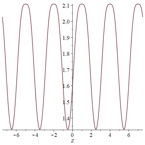
(a) $U(Z)$ for $-5{\omega}_{1}\leq Z\leq 5{\omega}_{1}$.

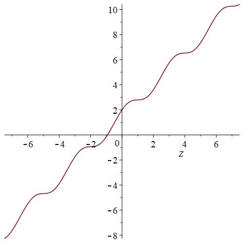
(b) $z(Z)$ for $-5{\omega}_{1}\leq Z\leq 5{\omega}_{1}$.

Figure 1: Parametric form of mCH travelling waves for real $Z$.

Example 2.3.

To illustrate the preceding theorem, we use it to plot a particular travelling wave solution of (1.1) which is bounded and real for $x,t\in{\mathbb{R}}$. We choose a Weierstrass cubic defined by fixing the values of the invariants, and also make a choice of the parameter $W$, taking

$$g_{2}=4,\qquad g_{3}=-1,\qquad W=1.$$

From (2.40) and (2.38) this gives the value of the velocity of the travelling wave and the other constants appearing in the solution as

$$c\approx 4.494929942,\qquad\tilde{c}\approx 0.298653316,\qquad\tilde{k}\approx 2.107492133.$$

In this case, the Weierstrass $\wp$ function has real/imaginary half-periods given by

$${\omega}_{1}\approx 1.496729323,\qquad{\omega}_{2}\approx 1.225694691\mathrm{i},$$

respectively, so taking the third half-period ${\omega}_{3}={\omega}_{1}+{\omega}_{2}$, the function $\wp(Z+{\omega}_{3})$ is real-valued, bounded and periodic with real period $2{\omega}_{1}$ for $Z\in{\mathbb{R}}$. Thus, to avoid poles for real values of $Z$, we can exploit the freedom to shift $Z$ and $z$ in Theorem 2.2, replacing $Z\to Z+{\omega}_{3}$ in (2.37) and (2.42), and choosing the arbitrary constant in the latter so that $z$ is real for all $Z\in{\mathbb{R}}$. This guarantees that $U$ given by (2.41) is a bounded periodic function for real argument $Z$, and the corresponding function $U(z)$ defined parametrically by $z(Z)$ is a bounded periodic solution of (2.24). Indeed, from the quasiperiodicity of the Weierstrass sigma function, which in particular means that ${\sigma}(Z+2{\omega}_{1})=-e^{2(Z+{\omega}_{1}){\zeta}({\omega}_{1})}{\sigma}(Z)$, it follows from (2.42) that the period of $U(z)$ is given by

$$z(Z+2{\omega}_{1})-z(Z)=4\big{(}{\omega}_{1}{\zeta}(W)-W{\zeta}({\omega}_{1})\big{)}\approx 3.734925095$$

in this particular numerical example.

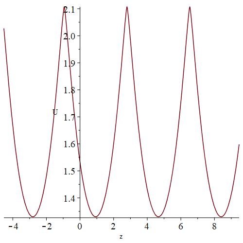
Figure 2: Periodic travelling wave solution of the mCH equation.

Moreover, in this case we find that $\tilde{v}(Z)$ is positive for all real $Z$, so $\genfrac{}{}{}{2}{\mathrm{d}z}{\mathrm{d}Z}=2\tilde{v}>0$ and $z(Z)$ is a monotone increasing function of its argument, as is visible from the right-hand panel of Fig.1. We have also plotted $U$ against $Z$ in the left-hand panel of the latter figure, where both plots are for $-5{\omega}_{1}\leq Z\leq 5{\omega}_{1}$, while in Fig.2 we have plotted $U$ against $z$, in the range $-3{\omega}_{1}\leq Z\leq 4{\omega}_{1}$, corresponding to the travelling wave profile for the mCH equation. Although the periodic peaks in this figure appear somewhat sharp, a closer look reveals that the solution is smooth for all real $z$. However, by suitably adapting the technique used in [30], it should be possible to obtain a single (weak) peakon solution from this family of periodic solutions, by taking a double scaling limit where the real period $2{\omega}_{1}\to\infty$ and the background (minimum) value of $U$ tends to zero.

2.3 Scaling similarity solutions

The mCH equation (1.1) has a one-parameter family of similarity solutions given by taking

$$u(x,t)=t^{-\genfrac{}{}{}{2}{1}{2}}U(z),\qquad m(x,t)=t^{-\genfrac{}{}{}{2}{1}{2}}M(z),\qquad z=x+{\alpha}\log t.$$ (2.43)

These solutions generalize the separable solutions (1.10), which arise when the parameter ${\alpha}=0$. Upon substituting the expressions (2.43) into the mCH equation (1.1), or equivalently into (1.6), we find

$$({\alpha}+U^{2}-U_{z}^{2})M_{z}+(2U_{z}M-\genfrac{}{}{}{2}{1}{2})M=0,\qquad M=U-U_{zz},$$ (2.44)

where the latter is a compact way of writing the corresponding autonomous ODE of third order for $U(z)$, that is

$$(U_{z}^{2}-U^{2}-{\alpha})(U_{zzz}-U_{z})+2U_{z}(U_{zz}-U)^{2}+\genfrac{}{}{}{2}{1}{2}(U_{zz}-U)=0.$$ (2.45)

In order to obtain parametric formulae for the solutions of (2.45), we proceed to apply the reciprocal transformation (2.6) to the similarity solutions (2.43). Without loss of generality we can fix

$$T=4t\implies\mathrm{d}\log T=\mathrm{d}\log t,$$ (2.46)

and then we find that, under the reciprocal transformation, the reductions (2.43) correspond to scaling similarity reductions of the first negative mKdV flow, obtained by taking

$$u=2T^{-\genfrac{}{}{}{2}{1}{2}}U(Z),\quad m=2T^{-\genfrac{}{}{}{2}{1}{2}}M(Z),\quad f=4T^{-1}F(Z),\quad Z=XT^{\genfrac{}{}{}{2}{1}{2}}.$$ (2.47)

Indeed, applying the reduction (2.47) directly to the conservation law (2.8) with $v=m^{-1}$ produces

$$\frac{\mathrm{d}}{\mathrm{d}Z}\big{(}\genfrac{}{}{}{2}{1}{2}ZM^{-1}\big{)}=\frac{\mathrm{d}F}{\mathrm{d}Z}\implies\genfrac{}{}{}{2}{1}{2}ZM^{-1}-F=\mathrm{const},$$

and if we identify the integration constant above with the parameter ${\alpha}$ then this yields the relation

$$M(F+{\alpha})=\genfrac{}{}{}{2}{1}{2}Z.$$ (2.48)

To see that this is consistent with applying the reciprocal transformation to the solutions (2.43), note that from (2.48) and the relation (2.46) between $t$ and $T$ we have

$$\begin{array}[]{rcl}\mathrm{d}Z&=&T^{\genfrac{}{}{}{2}{1}{2}}\mathrm{d}X+\genfrac{}{}{}{2}{1}{2}T^{-\genfrac{}{}{}{2}{1}{2}}X\mathrm{d}T\\ &=&T^{\genfrac{}{}{}{2}{1}{2}}\mathrm{d}X+\genfrac{}{}{}{2}{1}{2}Z\,\mathrm{d}\log T\\ &=&T^{\genfrac{}{}{}{2}{1}{2}}(\genfrac{}{}{}{2}{1}{2}m\,\mathrm{d}x-\genfrac{}{}{}{2}{1}{2}mf\,\mathrm{d}t)+M(F+{\alpha})\,\mathrm{d}\log t\\ &=&T^{\genfrac{}{}{}{2}{1}{2}}(T^{-\genfrac{}{}{}{2}{1}{2}}M\,\mathrm{d}x-4T^{-\genfrac{}{}{}{2}{3}{2}}MF\,\mathrm{d}t)+M(F+{\alpha})\,\mathrm{d}\log t\\ &=&M(\mathrm{d}x+{\alpha}\,\mathrm{d}\log t)\\ &=&M\,\mathrm{d}z.\end{array}$$ (2.49)

As shown previously, the reduction (2.43) produces the ODE (2.44) with independent variable $z$, which can be rewritten in terms of $M$ and $F=U^{2}-U_{z}^{2}$ in the form

$$\frac{\mathrm{d}}{\mathrm{d}z}\Big{(}M(F+{\alpha})\Big{)}=\genfrac{}{}{}{2}{1}{2}M.$$

Then using the result of (2.49) to transform the derivatives according to $\genfrac{}{}{}{2}{\mathrm{d}}{\mathrm{d}z}=M\genfrac{}{}{}{2}{\mathrm{d}}{\mathrm{d}Z}$, the latter ODE becomes

$$\frac{\mathrm{d}}{\mathrm{d}Z}\Big{(}M(F+{\alpha})\Big{)}=\frac{1}{2},$$

that is precisely the outcome of differentiating each side of (2.48) with respect to $Z$.

Now from the definitions (2.7) and (1.4), we can write down corresponding relations for the similarity solutions (2.47), involving $Z$ derivatives, namely

$$F=U^{2}-\left(M\frac{\mathrm{d}U}{\mathrm{d}Z}\right)^{2},\qquad M=U-\left(M\frac{\mathrm{d}}{\mathrm{d}Z}\right)^{2}U,$$

and then from (2.10) we obtain

$$\frac{\mathrm{d}F}{\mathrm{d}Z}=2M\frac{\mathrm{d}U}{\mathrm{d}Z},$$ (2.50)

so we can eliminate derivatives of $U$ from the previous identities, to find

$$U^{2}=\tfrac{1}{4}F_{Z}^{2}+F,\qquad U=M\big{(}\genfrac{}{}{}{2}{1}{2}F_{ZZ}+1\big{)}.$$ (2.51)

Upon comparing the two equations for $U$ above, and using (2.48) to write $M$ in terms of $F$, we obtain a single ODE of second order and second degree satisfied by $F$, that is

$$\left(\frac{1}{2}\frac{\mathrm{d}^{2}F}{\mathrm{d}Z^{2}}+1\right)^{2}=\frac{(F+{\alpha})^{2}}{Z^{2}}\left(\Big{(}\frac{\mathrm{d}F}{\mathrm{d}Z}\Big{)}^{2}+4F\right),$$ (2.52)

which is a non-autonomous analogue of (2.31).

If we introduce $\tilde{v}=\tilde{v}(Z)$ according to

$$\tilde{v}=M^{-1}=2Z^{-1}(F+{\alpha}),$$ (2.53)

so that

$$v(X,T)=\tfrac{1}{2}T^{\genfrac{}{}{}{2}{1}{2}}\tilde{v}(Z),$$ (2.54)

then the direct similarity reduction of (2.13) is an ODE of third order for $\tilde{v}$, given by

$$\frac{\mathrm{d}}{\mathrm{d}Z}\left(\tilde{v}^{-1}\Big{(}\frac{\mathrm{d}^{2}}{\mathrm{d}Z^{2}}(Z\tilde{v})+4\Big{)}\right)=\tilde{v}\frac{\mathrm{d}}{\mathrm{d}Z}\big{(}Z\tilde{v}\big{)}.$$ (2.55)

However, unlike the case of travelling waves, the above equation cannot be integrated to yield an analogue of (2.33) that is first degree in $\tilde{v}_{ZZ}$; instead, $\tilde{v}$ satisfies a non-autonomous equation of second order and second degree, obtained from (2.52) by replacing $F$ and its derivatives, using

$$F=\tfrac{1}{2}Z\tilde{v}-{\alpha},$$ (2.56)

which follows from (2.53).

We now proceed to show how $F(Z)$ satisfying (2.52), or equivalently $\tilde{v}(Z)$, is given in terms of a solution of a particular case of Painlevé III, that is

$$\frac{\mathrm{d}^{2}P}{\mathrm{d}Z^{2}}=\frac{1}{P}\left(\frac{\mathrm{d}P}{\mathrm{d}Z}\right)^{2}-\frac{1}{Z}\left(\frac{\mathrm{d}P}{\mathrm{d}Z}\right)+\frac{1}{Z}\big{(}2P^{2}+a)-\frac{1}{P},$$ (2.57)

for a suitable choice of the parameter $a$. If we identify $P\to w$ and $Z\to{\zeta}$, then this is equation (1.12) with parameters

$$\tilde{{\alpha}}=2,\quad\tilde{{\beta}}=a,\quad\tilde{{\gamma}}=0,\quad\tilde{\delta}=-1.$$

The main point is that, as described in [3] (and originally derived in [25]), the ODE (2.57) arises as the equation for scaling similarity reductions of the negative KdV flow (2.3), so by applying the result of Proposition 2.1 to these reductions, a link with (2.52) follows. Under the reduction (2.43) applied to (2.15) with $v(X,T)=\genfrac{}{}{}{2}{1}{2}T^{\genfrac{}{}{}{2}{1}{2}}M^{-1}=\genfrac{}{}{}{2}{1}{2}T^{\genfrac{}{}{}{2}{1}{2}}\tilde{v}$, we find

$$p(X,T)=T^{-\genfrac{}{}{}{2}{1}{2}}P(Z),$$ (2.58)

where $P=P(Z)$ is given in terms of $\tilde{v}$ by

$$P=\frac{1}{\tilde{v}}\left(\frac{1}{4}\frac{\mathrm{d}^{2}}{\mathrm{d}Z^{2}}\big{(}Z\tilde{v}\big{)}+1\right)-\frac{1}{4}\frac{\mathrm{d}}{\mathrm{d}Z}\big{(}Z\tilde{v}\big{)},$$ (2.59)

or equivalently, using (2.53), it can be rewritten in terms of $F$ as

$$P=\frac{Z}{2(F+{\alpha})}\left(\frac{1}{2}\frac{\mathrm{d}^{2}F}{\mathrm{d}Z^{2}}+1\right)-\frac{1}{2}\frac{\mathrm{d}F}{\mathrm{d}Z}.$$ (2.60)

Since we know from [3] that if $p(X,T)$ satisfying (2.3) has the form (2.58) then $P(Z)$ is a solution of (2.57) for some $a$, the question is how to determine this parameter. It is convenient to note that (2.59) or (2.60) can be expressed in the form

$$P=U-\tfrac{1}{2}F_{Z},$$ (2.61)

and also observe that (2.50) is equivalent to the formula

$$U_{Z}=\tfrac{1}{2}\tilde{v}F_{Z}.$$

Then applying $\genfrac{}{}{}{2}{\mathrm{d}}{\mathrm{d}Z}$ to (2.61) together with the second equation in (2.51) implies that

$$P_{Z}=U_{Z}-\tfrac{1}{2}F_{ZZ}=\tfrac{1}{2}\tilde{v}F_{Z}+1-\tilde{v}U\implies P_{Z}-1=\tilde{v}\big{(}\tfrac{1}{2}F_{Z}-U\big{)}=-\tilde{v}P.$$

Hence we obtain the following expression for $\tilde{v}$ in terms of $P$:

$$\tilde{v}=-\frac{(P_{Z}-1)}{P}.$$ (2.62)

This also follows directly by applying the similarity reduction to the formula (2.16), taking the scaling (2.54) into account, and it leads to the relation between the solutions of (2.52) and (2.57).

Lemma 2.4.

There is a one-to-one correspondence between solutions of (2.52) and (2.57), with the parameters related by

$$a=2{\alpha}+1,$$ (2.63)

where $P$ is given in terms of $F$ by (2.60), and $F$ is given in terms of $P$ by

$$F=-\frac{Z}{2P}\left(\frac{\mathrm{d}P}{\mathrm{d}Z}-1\right)-{\alpha}.$$ (2.64)

• The relation (2.64) for $F$ is an immediate consequence of (2.62) and (2.56), and can be rewritten as

  $$F=-\tfrac{1}{2}Z{\Lambda}_{Z}+\tfrac{Z}{2}P^{-1}-{\alpha},\qquad\mathrm{with}\quad{\Lambda}_{Z}=\tfrac{\mathrm{d}}{\mathrm{d}Z}\log P,$$

  where the latter notation allows the Painlevé III equation (2.57) to be expressed as

  $$\frac{\mathrm{d}}{\mathrm{d}Z}\big{(}Z{\Lambda}_{Z}\big{)}=2P+aP^{-1}-ZP^{-2}.$$

  Using this form of the ODE for $P$ to eliminate terms in ${\Lambda}_{ZZ}=\genfrac{}{}{}{2}{\mathrm{d}^{2}}{\mathrm{d}Z^{2}}\log P$, the derivatives of $F$ can be written as

  $$F_{Z}=-\tfrac{Z}{2}P^{-1}{\Lambda}_{Z}-P+\tfrac{1}{2}(1-a)P^{-1}+\tfrac{Z}{2}P^{-2},$$

  $$F_{ZZ}=\tfrac{Z}{2}P^{-1}{\Lambda}_{Z}^{2}-\big{(}P+\tfrac{1}{2}(1-a)P^{-1}+ZP^{-2}\big{)}{\Lambda}_{Z}-1+\tfrac{1}{2}(1-a)P^{-2}+\tfrac{Z}{2}P^{-3}.$$

  Upon substituting these expressions for $F$ and its derivatives into (2.52), almost all the terms cancel, and all that remains is

  $$\frac{1}{2}\big{(}{\Lambda}_{Z}-P^{-1}\big{)}^{2}(2{\alpha}+1-a)=0,$$

  from which (3.59) follows. ∎

In the description of the solutions of (2.45) in parametric form, it is convenient to make use of solutions of the ODE (2.57) connected via a Bäcklund transformation. For this case of the Painlevé III equation, given a solution $P=P(Z)$ with parameter value $a$, the quantities

$$P_{\pm}=\frac{Z\big{(}\pm P_{Z}+1\big{)}}{2P^{2}}+\frac{\big{(}\mp 1-a\big{)}}{2P}$$ (2.65)

are solutions of the same equation but with the parameter replaced by $a\pm 2$, respectively. It is also helpful to consider the form of the corresponding KdV field $V$ under the scaling similarity reduction (2.58), which takes the form

$$V(X,T)=T\bar{V}(Z),\qquad\bar{V}=-\frac{1}{4P^{2}}\left(\Big{(}\frac{\mathrm{d}P}{\mathrm{d}Z}\Big{)}^{2}-1\right)+\frac{1}{2ZP}\left(\frac{\mathrm{d}P}{\mathrm{d}Z}-2P^{2}-a\right),$$ (2.66)

where the above expression for $\bar{V}$ in terms of $P$ is found by applying the similarity reduction to the formula (2.5), and then using (2.57) to eliminate the $P_{ZZ}$ term. Then we introduce a tau function ${\sigma}_{a}(Z)$, in terms of which the scaled KdV field $\bar{V}$ is given by the standard KdV tau function relation

$$\bar{V}(Z)=2\frac{\mathrm{d}^{2}}{\mathrm{d}Z^{2}}\log{\sigma}_{a}(Z)$$ (2.67)

(invariant under gauge transformations of the form ${\sigma}_{a}(Z)\to\exp(AZ+B){\sigma}_{a}(Z)$). The index $a$ denotes the parameter value in the equation (2.57), so if we replace $P\to P_{\pm}$ and $a\to a\pm 2$ in the formula (2.66) for $\bar{V}$ then we obtain corresponding (scaled) KdV fields $\bar{V}_{\pm}$ and their associated tau functions, related by

$$\bar{V}_{\pm}(Z)=2\frac{\mathrm{d}^{2}}{\mathrm{d}Z^{2}}\log{\sigma}_{a\pm 2}(Z).$$

Remark 2.5.

In addition to a fixed singularity at $Z=0$, where solutions can have branching (see Example 2.7 below), there are two kinds of movable singularities that occur in (2.57) at points $Z_{0}\in{\mathbb{C}}$ with $Z_{0}\neq 0$: movable zeros, where $P$ has a local expansion

$$P(Z)=\pm(Z-Z_{0})+\frac{\pm 1-a}{2Z_{0}}(Z-Z_{0})^{2}+c_{3}(Z-Z_{0})^{3}+O\big{(}(Z-Z_{0})^{4}\big{)},\quad c_{3}\,\,\mathrm{arbitrary},$$

and movable poles, in the neighbourhood of which $P$ has the Laurent series

$$P(Z)=Z_{0}(Z-Z_{0})^{-2}+c_{0}-\frac{c_{0}}{Z_{0}}(Z-Z_{0})+O\big{(}(Z-Z_{0})^{2}\big{)},\quad c_{0}\,\,\mathrm{arbitrary}.$$

The reduced KdV field $\bar{V}$, given in terms of $P$ by (2.66), is regular at points where $P$ has movable zeros, since $\bar{V}(Z)=\mp\genfrac{}{}{}{2}{3}{2}c_{3}+O\big{(}(Z-Z_{0})\big{)}$ in the neighbourhood of such points; but at points where $P$ has double poles, $\bar{V}$ does also, having the local expansion

$$\bar{V}(Z)=-2(Z-Z_{0})^{-2}+\frac{c_{0}}{Z_{0}}+O\big{(}(Z-Z_{0})^{2}\big{)},$$

so from (2.67) the tau function vanishes at these points, being given by

$${\sigma}_{a}(Z)=C(Z-Z_{0})\Big{(}1+O\big{(}(Z-Z_{0})\big{)}\Big{)},\qquad C\neq 0,$$

where the constant $C$ depends on the choice of gauge.

Using loop group methods, Schiff constructed a Bäcklund transformation for the PDE (2.3) [39], and in [25] it was remarked that this arises naturally from the standard Darboux transformation for the Schrödinger operator. Furthermore, in the case of the scaling similarity solutions of (2.3) it corresponds to a Darboux transformation with zero eigenvalue, which is associated with the operator refactorization

$$D_{X}^{2}+V=(D_{X}-v)(D_{X}+v)\longrightarrow D_{X}^{2}+V^{*}=(D_{X}+v)(D_{X}-v),$$

and this reduces to the Bäcklund transformation (2.65) for the Painlevé III equation (2.57). In terms of the standard Miura formula (2.14), the latter transformation is achieved by replacing $v\to-v$; but more precisely, at the level of the scaling similarity reduction, taking into account the factors of 2 that appear in (2.47), a direct calculation shows that this transformation gives

$$\bar{V}=\tfrac{1}{2}\tilde{v}_{Z}-\tfrac{1}{4}\tilde{v}^{2}\longrightarrow\bar{V}_{-}=-\tfrac{1}{2}\tilde{v}_{Z}-\tfrac{1}{4}\tilde{v}^{2},\qquad a\to a-2.$$ (2.68)

Subtracting the expressions for $\bar{V}$ and $\bar{V}_{-}$ produces

$$\tilde{v}_{Z}=\bar{V}-\bar{V}_{-},$$

which leads to the usual expression for an mKdV field as the logarithmic derivative of a ratio of two tau functions: the scaled field $\tilde{v}$ is given by

$$\tilde{v}(Z)=2\frac{\mathrm{d}}{\mathrm{d}Z}\log\left(\frac{{\sigma}_{a}(Z)}{{\sigma}_{a-2}(Z)}\right)$$ (2.69)

(with an appropriate choice of gauge). This allows us to state the main result of this section.

Theorem 2.6.

The solutions of the ODE (2.45) for the similarity reduction (2.43) of the mCH equation (1.1) are given parametrically by $U=U(Z)$, $z=z(Z)$, where $U$ is defined by

$$U=\frac{Z}{2(F+{\alpha})}\left(\frac{1}{2}\frac{\mathrm{d}^{2}F}{\mathrm{d}Z^{2}}+1\right),$$ (2.70)

with $F(Z)$ being a solution of the ODE (2.52), related to a solution of the Painlevé III equation (2.57) with parameter $a=2{\alpha}+1$ by (2.64), and

$$z(Z)=2\log{\sigma}_{a}(Z)-2\log{\sigma}_{a-2}(Z)+\mathrm{const},$$ (2.71)

in terms of two Painlevé III tau functions ${\sigma}_{a}$, ${\sigma}_{a-2}$ connected via a Bäcklund transformation.

• The formula (2.70) follows from the second relation in (2.51) together with (2.53), while (2.71) comes from rearranging (2.49) as $\mathrm{d}z=M^{-1}\mathrm{d}Z=\tilde{v}\,\mathrm{d}Z$ and using (2.69) to integrate this. ∎

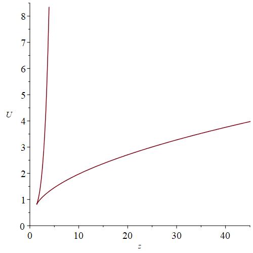
Figure 3: Plot of $U$ against $z$ for the parametric solution (2.76) with $0.02\leq{\zeta}\leq 4$.

Example 2.7.

It is instructive to consider an explicit example of the parametrization in Theorem 2.6. The equation (2.57) has a family of algebraic solutions for even integer values of the parameter $a$ (see [8] and references). The simplest such solution is given by

$$P=(Z/2)^{\genfrac{}{}{}{2}{1}{3}},\qquad a=0.$$ (2.72)

It is convenient to write all formulae in terms of ${\zeta}=(Z/2)^{\genfrac{}{}{}{2}{1}{3}}$, so that from (2.66) we have

$$P={\zeta}\implies\bar{V}=\tfrac{5}{144}{\zeta}^{-6}-\tfrac{1}{4}{\zeta}^{-2}.$$ (2.73)

The tau functions for some of these algebraic solutions are listed in Table 1 of [3], the relevant ones here being

$${\sigma}_{0}={\zeta}^{-\tfrac{5}{24}}\exp\big{(}-\tfrac{9}{8}{\zeta}^{4}\big{)},\qquad{\sigma}_{-2}={\zeta}^{\tfrac{7}{24}}\exp\big{(}-\tfrac{9}{8}{\zeta}^{4}-\tfrac{3}{2}{\zeta}^{2}\big{)}.$$ (2.74)

These generate the reduced mKdV field according to

$$\tilde{v}=\frac{\mathrm{d}}{\mathrm{d}Z}\log\left(\frac{{\sigma}_{0}}{{\sigma}_{-2}}\right)=\frac{1}{6}{\zeta}^{-2}\frac{\mathrm{d}}{\mathrm{d}{\zeta}}\log\left(\frac{{\sigma}_{0}}{{\sigma}_{-2}}\right)=-\frac{1}{6}{\zeta}^{-3}+{\zeta}^{-1},$$

so that the reduced KdV field as in (2.73) is given by

$$\bar{V}=\tfrac{1}{2}\tilde{v}_{Z}-\tfrac{1}{4}\tilde{v}^{2}=\tfrac{1}{12}{\zeta}^{-2}\tilde{v}_{\zeta}-\tfrac{1}{4}\tilde{v}^{2},$$

and from (2.56) the corresponding solution of (2.52) is found to be

$$F={\zeta}^{2}+\frac{1}{3},\qquad{\alpha}=-\frac{1}{2}.$$ (2.75)

Then from (2.70) and (2.71), using the form of $F$ in (2.75) above and the specific tau functions (2.74), the parametric form of the associated solution $U=U(z)$ of the ODE (2.45) with ${\alpha}=-\genfrac{}{}{}{2}{1}{2}$ is

$$U={\zeta}+\tfrac{1}{6}{\zeta}^{-1},\qquad z=3{\zeta}^{2}-\log{\zeta},$$ (2.76)

where here the solution is parametrized by ${\zeta}$ instead of $Z$, and a choice of arbitrary constant in $z$ has been set to zero. If we consider this solution for real ${\zeta}>0$, then it is clear that this similarity reduction of the mCH equation (1.1) has (at least) two real branches: in the limit of small positive ${\zeta}$, we have

$${\zeta}\to 0+\implies z\to\infty,\quad U\to\infty,$$

with asymptotics

$$U\sim\frac{1}{6}{\zeta}^{-1},\quad z\sim-\log{\zeta}\implies U\sim\frac{1}{6}e^{z},$$ (2.77)

while for large ${\zeta}$, we find

$${\zeta}\to\infty\implies z\to\infty,\quad U\to\infty,$$

but the asymptotic behaviour is completely different, namely

$$U\sim{\zeta},\quad z\sim 3{\zeta}^{2}\implies U\sim\sqrt{\frac{z}{3}}.$$

From the tangent vector

$$\left(\begin{array}[]{c}\genfrac{}{}{}{2}{\mathrm{d}z}{\mathrm{d}{\zeta}}\\ \genfrac{}{}{}{2}{\mathrm{d}U}{\mathrm{d}{\zeta}}\end{array}\right)=\left(\begin{array}[]{c}6{\zeta}-{\zeta}^{-1}\\ 1-\genfrac{}{}{}{2}{1}{6}{\zeta}^{-2}\end{array}\right)$$

we see that $\genfrac{}{}{}{2}{\mathrm{d}z}{\mathrm{d}{\zeta}}=0=\genfrac{}{}{}{2}{\mathrm{d}U}{\mathrm{d}{\zeta}}$ when ${\zeta}=1/\sqrt{6}$, corresponding to $(z,U)=\big{(}\genfrac{}{}{}{2}{1}{2}(1+\log 6),2/\sqrt{6}\big{)}$, where the two branches of the solution separate at a cusp, clearly visible in Fig.3. Note that the exponential asymptotics in (2.77) can be regarded as the leading term in an expansion $U\sim\genfrac{}{}{}{2}{1}{6}e^{z}+\sum_{n\geq 0}c_{n}e^{-nz}$ as $z\to\infty$, which is the sort of exponential series considered for Camassa-Holm type equations in [37].

3 Reductions of Novikov’s equation

This section is devoted to similarity reductions of Novikov’s equation (1.7), or equivalently (1.8). In due course we will need to compare its scaling similarity reductions to analogous reductions of the Degasperis-Procesi equation, so it will be convenient to rewrite (1.9) in the form of an associated conservation law for the field $p=m^{1/3}$, given by the system

$$\frac{\partial p}{\partial\bar{t}}+\frac{\partial}{\partial\bar{x}}(\bar{u}p)=0,\qquad p^{3}=(1-D_{\bar{x}}^{2})\bar{u},$$ (3.1)

where the other dependent/independent variables $u,x,t$ have been replaced by $\bar{u},\bar{x},\bar{t}$. In the rest of this section we reserve $m,u,x,t$ for the corresponding dependent/independent variables in Novikov’s equation (1.8).

3.1 Negative Kaup-Kupershmidt and Sawada-Kotera flows

As is well known [19], each of the flows in the Kaup-Kupershmidt hierarchy (with dependent variable $V$) and in the Sawada-Kotera hierarchy (with dependent variable $\hat{V}$) arises as the compatibility condition of a linear system, whose $X$ part is given by the eigenvalue problem for a third order Lax operator, that is

$$D_{X}^{3}+4VD_{X}+2V_{X}=(D_{X}+v)D_{X}(D_{X}-v)\quad\mathrm{and}\quad D_{X}^{3}+\hat{V}D_{X}=(D_{X}-v)(D_{X}+v)D_{X},$$ (3.2)

respectively, where the operator factorizations above produce the Miura maps

$$V=-\tfrac{1}{2}v_{X}-\tfrac{1}{4}v^{2},\qquad\hat{V}=v_{X}-v^{2},$$ (3.3)

which relate each of these hierarchies to the same modified hierarchy with dependent variable $v$. (The choice of scale for the Kaup-Kupershmidt field $V$ in (3.2) differs by a factor of 2 from [19], but is taken for consistency with the form of the Lax pair derived in [11], and the results in [3].)

In terms of the field $p$, the reciprocal transformation associated with the Degasperis-Procesi conservation law (3.1) is identical to that for the Camassa-Holm case, that is

$$\mathrm{d}X=p\,\mathrm{d}\bar{x}-\bar{u}p\,\mathrm{d}\bar{t},\qquad\mathrm{d}T=\mathrm{d}\bar{t},$$ (3.4)

apart from the fact that $p$ has a different meaning. The result of applying this transformation (2.2) is a PDE of third order for $p=p(X,T)$ as a function of the new independent variables $X,T$, given in conservation form as

$$\frac{\partial}{\partial T}(p^{-1})+\frac{\partial}{\partial X}\big{(}p(\log p)_{XT}-p^{3}\big{)}=0.$$ (3.5)

The connection with the Kaup-Kupershmidt hierarchy is made manifest by rewriting (3.5) in the alternative form

$$\frac{\partial V}{\partial T}+\frac{3}{4}\frac{\partial}{\partial X}\big{(}p^{2}\big{)}=0,$$ (3.6)

where the quantity $V$ is defined in terms of $p$ by the same formula as in (2.5) above, and corresponds to the dependent variable appearing in the first of the third order Lax operators in (3.2); this is how (3.6) was first derived in [11]. The PDE (3.6) is a flow of weight $-1$ in the Kaup-Kupershmidt hierarchy.

As for Novikov’s equation (1.8), if we introduce the dependent variables

$$q=m^{2/3},\qquad r=um^{1/3},$$ (3.7)

then it has a conservation law with density $m^{\genfrac{}{}{}{2}{2}{3}}$, which can be written as

$$q_{t}+(r^{2})_{x}=0,\qquad q^{2}=r-q^{\genfrac{}{}{}{2}{1}{2}}\frac{\partial^{2}}{\partial x^{2}}\big{(}q^{-\genfrac{}{}{}{2}{1}{2}}r\big{)},$$ (3.8)

with the latter equation being (1.4) expressed in terms of $q$ and $r$. This conservation law is discussed in the context of the prolongation structure of the PDE in [40]. In order to relate this to the Sawada-Kotera hierarchy, it is necessary to introduce the reciprocal transformation

$$\mathrm{d}X=q\,\mathrm{d}{x}-r^{2}\,\mathrm{d}t,\qquad\mathrm{d}T=\mathrm{d}{t},$$ (3.9)

which produces the transformed system

$$\frac{\partial}{\partial T}(q^{-1})=\frac{\partial}{\partial X}\big{(}q^{-1}r^{2}\big{)},\qquad r_{XX}+\hat{V}r+1=0,$$ (3.10)

where

$$\hat{V}=-\frac{\big{(}\sqrt{q}\big{)}_{XX}}{\sqrt{q}}-\frac{1}{q^{2}}$$ (3.11)

corresponds to the dependent variable for the Sawada-Kotera hierarchy. As shown in [28], the system (3.10) is a flow of weight $-1$ in this hierarchy, arising as the compatibility condition for a Lax pair whose $X$ part is the eigenvalue problem for the second operator in (3.2). For the discussion that follows, it will sometimes be convenient to refer to a potential $\Phi$ associated with the conservation law in (3.10), so that

$$q^{-1}=\Phi_{X},\qquad r=\sqrt{\frac{\Phi_{T}}{\Phi_{X}}}.$$ (3.12)

Remark 3.1.

The second Miura formula in (3.3) defines $\hat{V}$ in terms of $v$, but the solution of the inverse problem of finding $v$ given $\hat{V}$ is not unique, because it involves the solution of a Riccati equation. However, if $\hat{V}$ is specified in terms of $q$ by the formula (3.11), then taking

$$v=-\frac{1}{2}\big{(}\log q\big{)}_{X}\pm\frac{1}{q}$$ (3.13)

gives a particular solution for $v$, valid with either choice of sign above.

3.2 Travelling waves

The travelling wave solutions of the Degasperis-Procesi equation (1.9) were described in parametric form in [3]. They are given in terms of a parameter $Z$ which corresponds to the similarity variable for travelling waves of the PDE (3.5) with velocity $d$, which take the form $p(X,T)=P(Z)$, where $Z=X-dT$ and (up to the freedom to shift $Z\to Z+\,$const)

$$P=\frac{1}{{\alpha}\wp^{\prime}(W_{1})}\left(\frac{\wp(Z)-\wp(W_{1})}{\wp(Z)-\wp(W_{2})}\right),\qquad d=-\frac{16\wp^{\prime}(W_{2})^{6}}{\wp^{\prime}(W_{1})^{2}\wp^{\prime\prime}(W_{2})^{4}},$$ (3.14)

with constant parameters $W_{1},W_{2}$ related via

$${\alpha}=-\genfrac{}{}{}{2}{1}{2}\wp^{\prime\prime}(W_{2})/\wp^{\prime}(W_{2})^{2}=\big{(}\wp(W_{1})-\wp(W_{2})\big{)}^{-1}.$$ (3.15)

The corresponding velocity for the travelling waves of (1.9) is also given by an expression in terms of the Weierstrass $\wp$ function and its derivatives with these constants as arguments; see [3] for details.

The travelling waves for Novikov’s equation (1.8) were reduced to a quadrature in [28], given as a sum of two elliptic integrals of the third kind. Here we derive an explicit parametric form of these travelling wave solutions, which are found by imposing the reduction

$$u(x,t)=U(z),\qquad m(x,t)=M(z),\qquad z=x-ct$$ (3.16)

in (1.8), and noting that with

$$q(x,t)=Q(z),\qquad r(x,t)=R(z),$$

the conservation law in (3.8) integrates to yield

$$-cQ+R^{2}=\mathrm{const}.$$

Then, in a similar way to the case of mCH travelling waves treated in the previous section, we can relate these solutions with corresponding travelling waves of the reciprocally transformed system (3.10) with velocity $\tilde{c}$, which we can identify (up to a sign) with the integration constant above, to find

$$cQ=R^{2}+\tilde{c},$$ (3.17)

in terms of $Z=X-\tilde{c}T$, with $Q=Q(Z)$ and $R=R(Z)$ related by

$$\frac{R_{ZZ}+1}{R}=\frac{\big{(}\sqrt{Q}\big{)}_{ZZ}}{\sqrt{Q}}+\frac{1}{Q^{2}},$$ (3.18)

using the reduction of (3.11) with $\hat{V}\to\hat{V}(Z)$. To see this, note that for the travelling wave solutions of the negative Sawada-Kotera flow, the first equation in (3.10) becomes

$$-\tilde{c}\frac{\mathrm{d}}{\mathrm{d}Z}\big{(}Q^{-1}\big{)}=\frac{\mathrm{d}}{\mathrm{d}Z}\big{(}Q^{-1}R^{2}\big{)},$$

which integrates to give (3.17), with $c$ now playing the role of an integration constant. Upon using (3.17) with the assumption $c\neq 0$ to eliminate $Q$ from (3.18), an ODE of second order for $R(Z)$ is obtained, that is

$$\tilde{c}\left(\frac{R_{ZZ}}{R^{2}+\tilde{c}}-\frac{RR_{Z}^{2}}{(R^{2}+\tilde{c})^{2}}\right)=\frac{c^{2}R}{(R^{2}+\tilde{c})^{2}}-1,$$

and this can be integrated to produce the first order equation

$$\tilde{c}\left(\frac{\mathrm{d}R}{\mathrm{d}Z}\right)^{2}+2(R-e)(R^{2}+\tilde{c})+c^{2}=0,$$ (3.19)

with $e$ being another constant. The travelling wave reduction of (3.10) corresponds to the potential in (3.12) being of the form $\Phi(X,T)=\varphi(Z)+cT$.

Up to the freedom to shift $Z$ by an arbitrary amount $Z_{0}$, so that $Z\to Z-Z_{0}$, the general solution of (3.19) for $\tilde{c}\neq 0$ is an elliptic function of $Z$ given by

$$R(Z)=-2\tilde{c}\big{(}\wp(Z)-\wp(W)\big{)},$$ (3.20)

where $W$ is a constant such that

$$\tilde{c}=\frac{1}{2\wp^{\prime\prime}(W)},\qquad\frac{e}{\tilde{c}}=6\wp(W),$$ (3.21)

and the other constant appearing in the ODE satisfies

$$\frac{c^{2}}{4\tilde{c}^{3}}=6\wp(W)\wp^{\prime\prime}(W)-\wp^{\prime}(W)^{2}.$$ (3.22)

Hence, up to shifting the argument by $Z_{0}$, the solution $R(Z)$ is completely specified by the value of the parameter $W$ and the two invariants $g_{2},g_{3}$ of the Weierstrass $\wp$ function.

By applying the reciprocal transformation (3.9) to the travelling waves of (1.8), and using the relation (3.17), a short calculation analogous to (2.27) shows that these are related to the travelling wave reduction of (3.10) by the hodograph transformation

$$\mathrm{d}Z=Q\,\mathrm{d}z,$$ (3.23)

where each of the parameters $c,\tilde{c}$ has a complementary role as a wave velocity/integration constant, which switches according to whether the reduction of (1.8) or (3.10) is being considered. For further analysis of (3.23), we will also need to write the reciprocal of $Q$ in the form

$$\frac{1}{Q(Z)}=\frac{1}{2}\left(\frac{\wp^{\prime}(W_{+})}{\wp(Z)-\wp(W_{+})}+\frac{\wp^{\prime}(W_{-})}{\wp(Z)-\wp(W_{-})}\right),$$ (3.24)

where from (3.17) and (3.20) it follows that $1/Q(Z)$ has simple poles at values of $Z$ congruent to $\pm W_{\pm}\bmod{\Lambda}$ (with ${\Lambda}$ denoting the period lattice of the $\wp$ function), which are determined from the requirements

$$\wp(W_{+})+\wp(W_{-})=2\wp(W),\qquad\wp(W_{+})\wp(W_{-})=\wp(W)^{2}+\frac{1}{4\tilde{c}}.$$ (3.25)

These two equations for $\wp(W_{\pm})$ together imply that

$$\big{(}\wp(W_{+})-\wp(W_{-})\big{)}^{2}=-\frac{1}{\tilde{c}}.$$ (3.26)

Then from evaluating $\genfrac{}{}{}{2}{\mathrm{d}R}{\mathrm{d}Z}$ at $Z=W_{\pm}$ and using (3.19) together with the fact that $R^{2}+\tilde{c}=0$ at these points, we find that

$$\wp^{\prime}(W_{+})^{2}=\wp^{\prime}(W_{-})^{2}=-\frac{c^{2}}{4\tilde{c}^{3}};$$

thus from (3.26) we can fix signs so that

$$\wp^{\prime}(W_{+})=-\wp^{\prime}(W_{-})=\frac{c}{2\tilde{c}^{2}}\big{(}\wp(W_{+})-\wp(W_{-})\big{)}^{-1},$$ (3.27)

which ensures that $1/Q(Z)$ has residue $1/2$ at points congruent to $W_{\pm}\bmod{\Lambda}$, and residue $-1/2$ at points congruent to $-W_{\pm}\bmod{\Lambda}$, as in the formula (3.24).

Theorem 3.2.

The smooth travelling wave solutions (3.16) of Novikov’s equation (1.7) are given parametrically by $U=U(Z)$, $z=z(Z)$, where

$$U(Z)=\frac{\pm\sqrt{c}\,R(Z)}{\sqrt{R(Z)^{2}+\tilde{c}}}$$ (3.28)

with $R(Z)$ defined by (3.20) (up to the freedom to shift $Z\to Z+\,$const), and

$$z(Z)=\tfrac{1}{2}\log\left(\frac{{\sigma}(Z-W_{+}){\sigma}(Z-W_{-})}{{\sigma}(Z+W_{+}){\sigma}(Z+W_{-})}\right)+\big{(}{\zeta}(W_{+})+{\zeta}(W_{-})\big{)}Z+\mathrm{const},$$ (3.29)

with the parameters being specified by (3.21) and (3.22), together with (3.25) and (3.27).

• The definition of $q$ and $r$ in (3.7) implies that $u^{2}=r^{2}/q$, so reducing to the travelling wave solutions and taking a square root produces

  $$U=\pm\frac{R}{\sqrt{Q}},$$

  where either choice of sign is valid. (The PDE (1.7) is invariant under $u\to-u$.) Upon using (3.17) to replace $Q$ in terms of $R$, the expression (3.28) results. As for the formula (3.29), this follows from (3.23), using (3.24) and standard identities for Weierstrass functions to perform the integral $z=\int Q(Z)^{-1}\,\mathrm{d}Z+\,$const. ∎

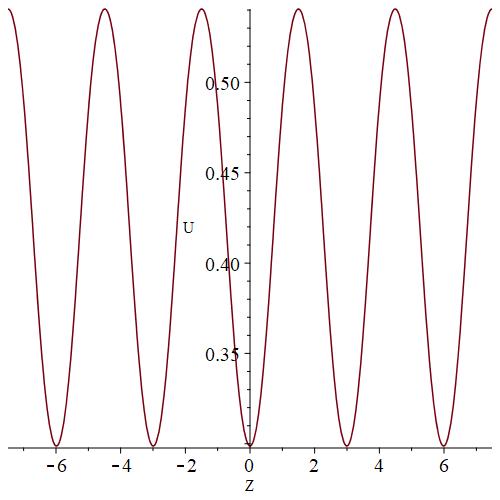
(a) $U(Z)$ for $-5{\omega}_{1}\leq Z\leq 5{\omega}_{1}$.

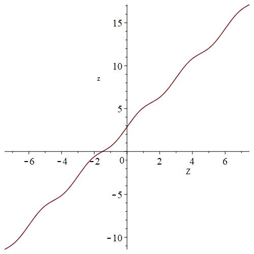
(b) $z(Z)$ for $-5{\omega}_{1}\leq Z\leq 5{\omega}_{1}$.

Figure 4: Parametric form of travelling waves for Novikov’s equation with real $Z$.

Example 3.3.

For illustration of the above theorem, we use it to plot a particular travelling wave solution of (1.7) which is bounded and real for $x,t\in{\mathbb{R}}$. We choose the same Weierstrass cubic as in Example 2.3 by fixing the values of the invariants as before, but make a different choice of the parameter $W$, with an exact value of $\wp(W)$, namely

$$g_{2}=4,\qquad g_{3}=-1,\qquad\wp(W)=1,$$

which arises from taking $W\approx 1.134273216$. In this case, $\wp^{\prime}(W)=-1$ and $\wp^{\prime\prime}(W)=4$, so from (3.21) and (3.22) this gives the value of the velocity of the travelling wave and the other constants appearing in the solution as

$$c=\frac{\sqrt{23}}{8\sqrt{2}},\qquad\tilde{c}=\frac{1}{8},\qquad e=\frac{3}{4}.$$

As before, we take three half-periods for the Weierstrass $\wp$ function given by

$${\omega}_{1}\approx 1.496729323,\qquad{\omega}_{2}\approx 1.225694691\mathrm{i},\qquad{\omega}_{3}={\omega}_{1}+{\omega}_{2},$$

and avoid poles for real values of $Z$, by exploiting the freedom to shift $Z$ and $z$ by constants in Theorem 3.2, replacing $Z\to Z+{\omega}_{3}$ in (3.20) and (3.29), and ensuring that $z$ is real for all $Z\in{\mathbb{R}}$ by an appropriate choice of constant in (3.29). Note that in this case we have

$$\wp(W_{\pm})=1\pm\sqrt{2}\mathrm{i},$$

and we can choose $W_{\pm}$ to be complex conjugates of one another, so that

$$W_{+}=\overline{W}_{-}\approx 0.6575861671-0.3645241628\mathrm{i},$$

and $\wp^{\prime}(W_{+})=-\sqrt{23}\mathrm{i}$ in accordance with (3.27). Then $U$ given by (3.28) is a bounded periodic function for real argument $Z$, and the corresponding function $U(z)$ defined parametrically by $z(Z)$ is a bounded periodic travelling wave profile for (1.7). Indeed, using the quasiperiodicity of the Weierstrass sigma function, the formula (3.29) shows that the period of $U(z)$ is

$$z(Z+2{\omega}_{1})-z(Z)=2\Big{(}{\omega}_{1}\big{(}{\zeta}(W_{+})+{\zeta}(W_{-})\big{)}-(W_{+}+W_{-}){\zeta}({\omega}_{1})\Big{)}\approx 5.708708303$$

in this numerical example.

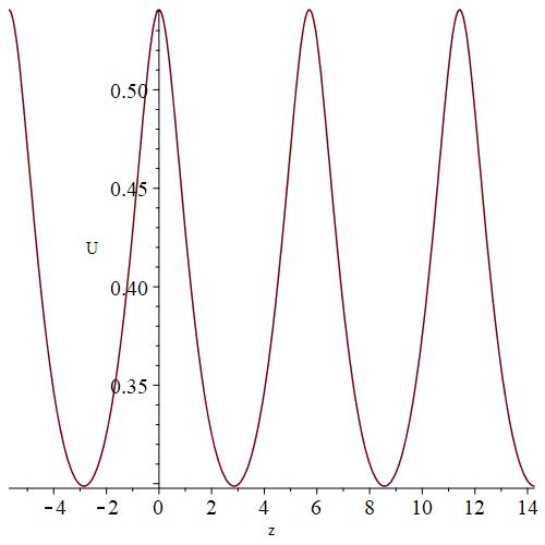
Figure 5: Periodic travelling wave solution of Novikov’s equation.

Clearly, in this case we have $Q(Z)=c^{-1}\big{(}R(Z)^{2}+\tilde{c}\big{)}>0$ for all real $Z$, so $\genfrac{}{}{}{2}{\mathrm{d}z}{\mathrm{d}Z}=1/Q>0$ and $z(Z)$ is a monotone increasing function of its argument, as is visible from the right-hand panel of Fig.4. The left-hand panel of the latter figure shows $U$ plotted against $Z$, where both plots are for $-5{\omega}_{1}\leq Z\leq 5{\omega}_{1}$, while in Fig.5 we have plotted $U$ against $z$, in the range $-3{\omega}_{1}\leq Z\leq 4{\omega}_{1}$, corresponding to the travelling wave profile for Novikov’s equation.

Remark 3.4.

Thus far we have not discussed how the result of Theorem 3.2, which describes the travelling waves of Novikov’s equation (1.7), is related to the travelling waves of the Degasperis-Procesi equation (1.9). The connection between them is somewhat indirect, arising from the two reciprocal transformations (3.4) and (3.9), together with the two Miura maps (3.3), and their reductions to the travelling wave solutions. On the one hand, as shown in [3], for the travelling wave solution (3.14) of (3.5), or equivalently (3.6), there is a corresponding Kaup-Kupershmidt field $V=V(Z)=\genfrac{}{}{}{2}{3}{4}d^{-1}P(Z)^{2}+\,$const. From the formulae (3.15) together with (3.14), it is apparent that $V$ is an elliptic function of $Z$ with double poles only at points congruent to $\pm W_{2}$, with the leading order in the Laurent expansion at these points being $V(Z)=-\genfrac{}{}{}{2}{3}{4}(Z\mp W_{2})^{-2}+O(1)$, so fixing the value at $Z=0$ we find that it can be written in the form

$$V(Z)=-\genfrac{}{}{}{2}{3}{4}\wp(Z+W_{2})-\genfrac{}{}{}{2}{3}{4}\wp(Z-W_{2})-\genfrac{}{}{}{2}{3}{2}\wp(W_{2})+\genfrac{}{}{}{2}{3}{4}{\alpha}^{2}\wp^{\prime}(W_{2})^{2}$$ (3.30)

(but see equation (2.21) in [3] for another equivalent expression). On the other hand, from the formula (3.24) we can use (3.13) to produce a (reduced) modified field variable $v=v(Z)$ given by

$$\begin{array}[]{rcl}v(Z)&=&\frac{1}{2}\frac{\mathrm{d}}{\mathrm{d}Z}\log Q(Z)^{-1}+\frac{1}{Q(Z)}\\ &=&-\frac{1}{2}\left(\frac{\wp^{\prime}(Z)-\wp^{\prime}(W_{+})}{\wp(Z)-\wp(W_{+})}+\frac{\wp^{\prime}(Z)-\wp^{\prime}(W_{-})}{\wp(Z)-\wp(W_{-})}\right)\\ &=&2{\zeta}(Z)-{\zeta}(Z+W_{+})+{\zeta}(W_{+})-{\zeta}(Z+W_{-})+{\zeta}(W_{-}).\end{array}$$ (3.31)

(The latter form of $v(Z)$ arises from choosing the second term in (3.13) with a plus sign, and applying suitable elliptic function identities; choosing the minus sign instead just replaces $W_{\pm}\to-W_{\pm}$ in the above expression.) So to the solution (3.20) of the ODE (3.19) for travelling waves of the system (3.10) there corresponds a Sawada-Kotera field $\hat{V}=\hat{V}(Z)$ given by

$$\hat{V}(Z)=\frac{\mathrm{d}v}{\mathrm{d}Z}-v^{2}=-6\wp(Z)-6\wp(W),$$ (3.32)

where the preceding explicit formula is obtained by considering the leading terms in the Laurent expansions of $v(Z)$ around its simple poles at points congruent to $Z=0,-W_{+},-W_{-}\bmod{\Lambda}$, where it has residues $2,-1,-1$ respectively; then noting that consequently $\hat{V}(Z)$ has only double poles at points congruent to $Z=0$, with leading order $\hat{V}(Z)\sim-6Z^{-2}-3\big{(}\wp(W_{+})+\wp(W_{-})\big{)}$, and using (3.25), the final expression in (3.32) follows. Now by reducing the first Miura map in (3.3) to these travelling waves, there should be an associated Kaup-Kaupershmidt field $V(Z)$, which is found from

$$V(Z)=-\tfrac{1}{2}\frac{\mathrm{d}v}{\mathrm{d}Z}-\tfrac{1}{4}v^{2}=\tfrac{1}{4}\hat{V}(Z)-\tfrac{3}{4}\frac{\mathrm{d}v}{\mathrm{d}Z},$$

so inserting the expressions (3.31) and (3.32) this yields

$$V(Z)=-\genfrac{}{}{}{2}{3}{4}\wp(Z+W_{+})-\genfrac{}{}{}{2}{3}{4}\wp(Z+W_{-})-\genfrac{}{}{}{2}{3}{2}\wp(W).$$ (3.33)

The connection between the Degasperis-Procesi/Novikov travelling wave solutions is now established by showing that it is consistent to identify the two different formulae (3.30) and (3.33) for a Kaup-Kupershmidt field $V$. First of all, the precise form of these travelling waves is specified up to the freedom to shift the independent variable $Z$ by an arbitrary constant, so if we replace $Z\to Z-\genfrac{}{}{}{2}{1}{2}(W_{+}+W_{-})$ in (3.33), then the double poles in the solution are at points congruent to $\pm\genfrac{}{}{}{2}{1}{2}(W_{+}-W_{-})\in{\mathbb{C}}/{\Lambda}$. Hence, comparing with (3.30), we can identify

$$W_{2}=\tfrac{1}{2}(W_{+}-W_{-}).$$ (3.34)

As a consequence of the duplication formula for the $\wp$ function, doubling (3.34) gives

$$\wp(W_{+}-W_{-})=\wp(2W_{2})=-2\wp(W_{2})+\tfrac{1}{4}\left(\frac{\wp^{\prime\prime}(W_{2})}{\wp^{\prime}(W_{2})}\right)^{2},$$

while at the same time, the addition formula for $\wp$ together with (3.27) implies that

$$\wp(W_{+}-W_{-})=-\wp(W_{+})-\wp(W_{-}).$$

So combining the latter two results with (3.25) and the first expression for ${\alpha}$ in (3.15), we obtain the equality

$$\wp(W)=\wp(W_{2})-\tfrac{1}{2}{\alpha}^{2}\wp^{\prime}(W_{2})^{2},$$ (3.35)

which implies that we can identify the constant terms in the two formulae (3.30) and (3.33). Finally, for these two different expressions for $V$ to be compatible, we require that the independent variable $Z$ should be the same in each case: in (3.30) it is given by $X-dT$, while in (3.33) it is $X-\tilde{c}T$, so (assuming that $X,T$ are the same in both cases) this means that the two wave velocities should coincide. Then from (3.21) we may make use of (3.35) to write

$$\tilde{c}^{-1}=2\wp^{\prime\prime}(W)=12\wp(W)^{2}-g_{2}=12\big{(}\wp(W_{2})-\tfrac{1}{2}{\alpha}^{2}\wp^{\prime}(W_{2})^{2}\big{)}^{2}-g_{2},$$

so that

$$\tilde{c}^{-1}=2\wp^{\prime\prime}(W_{2})-12{\alpha}^{2}\wp(W_{2})\wp^{\prime}(W_{2})^{2}+3{\alpha}^{4}\wp^{\prime}(W_{2})^{4},$$ (3.36)

whereas from (3.14) and (3.15) we have

$$\begin{array}[]{rcl}d^{-1}&=&-{\alpha}^{4}\wp^{\prime}(W_{2})^{2}\wp^{\prime}(W_{1})^{2}\\ &=&-{\alpha}^{4}\wp^{\prime}(W_{2})^{2}\Big{(}\wp^{\prime}(W_{2})^{2}+4\big{(}\wp(W_{1})^{3}-\wp(W_{2})^{3}\big{)}-g_{2}\big{(}\wp(W_{1})-\wp(W_{2})\big{)}\Big{)},\end{array}$$ (3.37)

using the first order ODE for the $\wp$ function. Finally, the second expression for ${\alpha}$ in (3.15) allows us to substitute $\wp(W_{1})=\wp(W_{2})+{\alpha}^{-1}$ in (3.37), and then eliminate $g_{2}=12\wp(W_{2})^{2}-2\wp^{\prime\prime}(W_{2})$, followed by replacing $\wp^{\prime\prime}(W_{2})=-2{\alpha}\wp^{\prime}(W_{2})^{2}$ in the resulting formula for $d^{-1}$ and doing the same in (3.36), which results in

$$d^{-1}=-4{\alpha}\wp^{\prime}(W_{2})^{2}-12{\alpha}^{2}\wp(W_{2})\wp^{\prime}(W_{2})^{2}+3{\alpha}^{4}\wp^{\prime}(W_{2})^{4}=\tilde{c}^{-1};$$

so the wave velocities are the same, as required.

We have already briefly commented on the discrete symmetry associated with the choice of sign in (3.13), which at the level of the travelling wave reduction of (3.10) produces two different modified variables

$$v_{\pm}=-\genfrac{}{}{}{2}{1}{2}(\log Q)_{Z}\pm Q^{-1},$$ (3.38)

where $v_{+}$ is given by (3.31), and $v_{-}$ is given by the same formula but with $W_{+}\to-W_{+}$, $W_{-}\to-W_{-}$ throughout. The Miura map $\genfrac{}{}{}{2}{\mathrm{d}v_{\pm}}{\mathrm{d}Z}-v_{\pm}^{2}$ gives the same (reduced) Sawada-Kotera field $\hat{V}(Z)$, as can be observed directly from the elliptic function expression on the far right-hand side of (3.32): this is invariant under changing the signs of $W_{\pm}$. However, applying the other Miura map to $v_{\pm}$ produces two different reduced Kaup-Kupershmidt fields, namely

$$V_{\pm}(Z)=-\genfrac{}{}{}{2}{1}{2}\tfrac{\mathrm{d}v_{\pm}}{\mathrm{d}Z}-\genfrac{}{}{}{2}{1}{4}v_{\pm}^{2}=-\genfrac{}{}{}{2}{3}{4}\wp(Z\pm W_{+})-\genfrac{}{}{}{2}{3}{4}\wp(Z\pm W_{-})-\genfrac{}{}{}{2}{3}{2}\wp(W)$$ (3.39)

(with (3.33) just being the first of these). So far, in order to derive the results on parametric travelling waves in Theorem 3.2, we have not needed to make use of this discrete symmetry, but in the case of the scaling similarity solutions considered in the next subsection it will be a more vital ingredient.

3.3 Scaling similarity solutions

Novikov’s equation (1.7) has a one-parameter family of similarity solutions, for which both $u$ and the momentum density $m$ in (1.8) scale the same way, given by the same form of reduction as in the case of the mCH equation (1.1), that is

$$u(x,t)=t^{-\genfrac{}{}{}{2}{1}{2}}U(z),\qquad m(x,t)=t^{-\genfrac{}{}{}{2}{1}{2}}M(z),\qquad z=x+{\alpha}\log t.$$ (3.40)

This reduction results in an autonomous ODE of third order for $U(z)$, namely

$$(U^{2}+{\alpha})(U_{zzz}-U_{z})+(3UU_{z}-\genfrac{}{}{}{2}{1}{2})(U_{zz}-U)=0.$$ (3.41)

To obtain solutions of the latter ODE in parametric form, we will consider corresponding similarity solutions of the negative Sawada-Kotera flow (3.10), related via the reciprocal transformation (3.9). Under the reduction (3.40), the quantities $q,r$ given by (3.7), that appear in the associated conservation law (3.8), take the form

$$q(x,t)=t^{-\genfrac{}{}{}{2}{1}{3}}Q(z),\qquad r(x,t)=t^{-\genfrac{}{}{}{2}{2}{3}}R(z).$$ (3.42)

The system (3.10) has scaling similarity solutions given by taking

$$q(X,T)=T^{-\genfrac{}{}{}{2}{1}{3}}Q(Z),\qquad r(X,T)=T^{-\genfrac{}{}{}{2}{2}{3}}R(Z),\qquad Z=XT^{\genfrac{}{}{}{2}{1}{3}}.$$ (3.43)

Applying this similarity reduction means that the first equation in the system produces

$$\frac{1}{3}\frac{\mathrm{d}}{\mathrm{d}Z}\big{(}ZQ^{-1}\big{)}=\frac{\mathrm{d}}{\mathrm{d}Z}\big{(}R^{2}Q^{-1}\big{)},$$ (3.44)

while, using the definition of $\hat{V}$ in (3.11), the second equation becomes

$$\frac{(Q^{1/2})_{ZZ}}{Q^{1/2}}+\frac{1}{Q^{2}}=\frac{R_{ZZ}+1}{R}.$$ (3.45)

The equation (3.44) integrates to give

$$Q^{-1}\big{(}\genfrac{}{}{}{2}{1}{3}Z-R^{2}\big{)}=\mathrm{const}.$$

If we let ${\alpha}$ denote the integration constant above, then this gives

$${\alpha}Q=\frac{Z}{3}-R^{2},$$ (3.46)

and we find that this corresponds precisely to the image under the reciprocal transformation (3.9) of the similarity solutions (3.40) of Novikov’s equation (1.8), where (without loss of generality) we can set $t=T$ and perform a calculation analogous to (2.49) to find the hodograph transformation

$$\mathrm{d}Z=Q\,\mathrm{d}z,$$ (3.47)

so that the system consisting of (3.46) and (3.45) is a consequence of replacing the $z$ derivatives in (3.41) with $\genfrac{}{}{}{2}{\mathrm{d}}{\mathrm{d}z}=Q\genfrac{}{}{}{2}{\mathrm{d}}{\mathrm{d}Z}$ and rewriting suitable combinations of $U$ and its derivatives in terms of the quantities $Q$ and $R$.

Remark 3.5.

The form of the scaling similarity reduction (3.43) and the equation (3.46) arise from (3.12) by choosing a potential of the form

$$\Phi(X,T)=\varphi(Z)-{\alpha}\log T,\qquad Z=XT^{\genfrac{}{}{}{2}{1}{3}},$$

with $1/Q(Z)=\genfrac{}{}{}{2}{\mathrm{d}}{\mathrm{d}Z}\varphi(Z)$, so that integrating (3.47) gives $z=\varphi(Z)$, but in due course we will obtain a slightly more explicit formula for the potential $\varphi$ in terms of tau functions.

Guided by the results on travelling waves in the preceding subsection, we next use (3.46) with ${\alpha}\neq 0$ to substitute for $Q$ and $Q_{Z}={\alpha}^{-1}(\genfrac{}{}{}{2}{1}{3}-2RR_{Z})$, $Q_{ZZ}=-2{\alpha}^{-1}(RR_{ZZ}+R_{Z}^{2})$ in (3.45), to find a single ODE of second order for $R(Z)$, that is

$$\frac{\mathrm{d}^{2}R}{\mathrm{d}Z^{2}}=\frac{1}{R^{2}-\genfrac{}{}{}{2}{1}{3}Z}\left(R\left(\frac{\mathrm{d}R}{\mathrm{d}Z}\right)^{2}-\frac{R^{2}}{Z}\left(\frac{\mathrm{d}R}{\mathrm{d}Z}\right)+\frac{3}{Z}R^{4}-2R^{2}+\frac{(\genfrac{}{}{}{2}{1}{12}-3{\alpha}^{2})}{Z}R+\genfrac{}{}{}{2}{1}{3}Z\right).$$ (3.48)

The above equation is very similar in form to the Painlevé V equation (1.15), and indeed it is related to it by a simple change of dependent and independent variables.

Lemma 3.6.

The solutions $R=R(Z)$ of the ODE (3.48) are given by

$$R=\sqrt{\frac{Z}{3}}\left(\frac{1+w}{1-w}\right),$$ (3.49)

where $w=w({\zeta})$ is a solution of the Painlevé V equation (1.15) with parameters

$$\tilde{{\alpha}}=\genfrac{}{}{}{2}{1}{2}{\alpha}^{2},\quad\tilde{{\beta}}=-\genfrac{}{}{}{2}{1}{2}{\alpha}^{2},\quad\tilde{{\gamma}}=1,\quad\tilde{\delta}=0,$$ (3.50)

and

$${\zeta}=(4Z/3)^{\genfrac{}{}{}{2}{3}{2}}.$$ (3.51)

• To see this, note that the coefficient of $\big{(}\genfrac{}{}{}{2}{\mathrm{d}R}{\mathrm{d}Z}\big{)}^{2}$ in (3.48) is a rational function of $R$ of degree 2, with poles at $R=\pm\sqrt{\genfrac{}{}{}{2}{Z}{3}}$, so the ODE has fixed singularities at these points and at $R=\infty$, while the coefficient of $\big{(}\genfrac{}{}{}{2}{\mathrm{d}w}{\mathrm{d}{\zeta}}\big{)}^{2}$ in (1.15) is

  $$\frac{1}{2w}+\frac{1}{w-1}=\frac{3w-1}{2w(w-1)},$$ (3.52)

  which suggests transforming the dependent variable with the Möbius transformation (3.49). in order to move the fixed singularities to $w=0,1,\infty$. This transformation indeed produces the correct coefficient (3.52), transforming (3.48) to an equation with leading terms

  $$\frac{\mathrm{d}^{2}w}{\mathrm{d}Z^{2}}=\left(\frac{1}{2w}+\frac{1}{w-1}\right)\left(\frac{\mathrm{d}w}{\mathrm{d}Z}\right)^{2}+\cdots,$$

  and then to obtain the precise form of Painlevé V further requires a change of independent variables, namely the replacement

  $$Z=\frac{3}{4}{\zeta}^{\genfrac{}{}{}{2}{2}{3}},$$

  with inverse (3.51), which produces the equation (1.15) with the particular choice of coefficients (3.50). ∎

It is a result due to Gromak that Painlevé V with $\tilde{\delta}=0$ can be solved in terms of Painlevé III transcendents [22] (see also $\S 32.7$(vi) in [36]). If we replace the set of parameters in (1.12) with $(\hat{{\alpha}},\hat{{\beta}},\hat{{\gamma}},\hat{\delta})$, and denote the dependent and independent variables by $\hat{w},\eta$, respectively, then a more exact statement is that, if $\hat{w}=\hat{w}(\eta)$ is a solution of Painlevé III with parameters $(\hat{{\alpha}},\hat{{\beta}},1,-1)$, then $w=w({\zeta})$ with

$$w={\cal F}\Big{(}\hat{w},\tfrac{\mathrm{d}\hat{w}}{\mathrm{d}\eta},\eta,{\alpha}\Big{)},\qquad\eta=\sqrt{2{\zeta}},$$ (3.53)

satisfies Painlevé V with parameters given by

$$(\tilde{{\alpha}},\tilde{{\beta}},\tilde{{\gamma}},\tilde{\delta})=\Big{(}\genfrac{}{}{}{2}{1}{32}(\hat{{\beta}}-\varepsilon\hat{{\alpha}}+2)^{2},-\genfrac{}{}{}{2}{1}{32}(\hat{{\beta}}+\varepsilon\hat{{\alpha}}-2)^{2},-\varepsilon,0\Big{)},$$ (3.54)

where $\varepsilon=\pm 1$ and ${\cal F}$ is a certain rational function of its arguments (see $\S 32.7$(vi) in [36] for full details). We now wish to use Gromak’s result in order to show that the solutions of the ODE (3.48) are related to the scaling similarity solutions of the negative Kaup-Kupershmidt flow (3.6), which in turn correspond to solutions of the Degasperis-Procesi equation (1.9) via the reciprocal transformation (3.4). In [3] it was explained how the scaling similarity reduction of (3.6), or rather (3.5), results in an ODE which is equivalent to Painlevé III with parameter values

$$(\hat{{\alpha}},\hat{{\beta}},\hat{{\gamma}},\hat{\delta})=(0,\genfrac{}{}{}{2}{4}{3}a,1,-1),$$ (3.55)

where $a$ is arbitrary. However, applying the transformation (3.53) directly to the latter solutions with $\hat{{\alpha}}=0$ does not lead to solutions of Painlevé V with $\tilde{{\alpha}}=-\tilde{{\beta}}$, which is what we require from (3.50). Thus, in order to obtain the required connection, we can apply one of the Bäcklund transformations for Painlevé III (see e.g. [4]), which sends

$$(\hat{{\alpha}},\hat{{\beta}},1,-1)\longrightarrow(\hat{{\alpha}}-2,\hat{{\beta}}+2,1,-1).$$ (3.56)

Then starting from the parameter values (3.55) and applying (3.56) followed by the transformation (3.53) in the case $\varepsilon=-1$, a solution of Painlevé V with the appropriate parameters arises.

For the similarity reductions of Novikov’s equation, it is more convenient to describe these connections directly in terms of the solutions of the ODE

$$\frac{\mathrm{d}^{2}P}{\mathrm{d}Z^{2}}=\frac{1}{P}\left(\frac{\mathrm{d}P}{\mathrm{d}Z}\right)^{2}-\frac{1}{Z}\left(\frac{\mathrm{d}P}{\mathrm{d}Z}\right)+\frac{1}{Z}\big{(}3P^{3}+a)-\frac{1}{P},$$ (3.57)

which was derived in [3] by taking scaling similarity solutions of (3.5), of the form

$$p(X,T)=T^{-1/3}P(Z),\qquad Z=XT^{1/3}.$$ (3.58)

Proposition 3.7.

Each solution $P=P(Z)$ of the ODE (3.57) with parameter

$$a=-\tfrac{3}{2}\pm 3{\alpha}$$ (3.59)

provides a solution $R=R(Z)$ of (3.48) with parameter ${\alpha}$, via the formula

$$R=\frac{Z(P_{Z}+1)}{3P^{2}}-\frac{(a+1)}{3P},$$ (3.60)

and conversely, each solution of (3.48) provides a solution of (3.57) with parameter $a$ given by (3.59), according to the formula

$$P=-\frac{ZR_{Z}+(\pm 3{\alpha}-\genfrac{}{}{}{2}{1}{2})R}{3R^{2}-Z}.$$ (3.61)

• The ODE (3.57) corresponds to Painlevé III with parameter values (3.55), via the transformation

  $$\hat{w}(\eta)=(Z/3)^{-\genfrac{}{}{}{2}{1}{4}}P(Z),\qquad\eta=4(Z/3)^{\genfrac{}{}{}{2}{3}{4}},$$ (3.62)

  as given (with slightly different notation) in equation (3.21) in [3]. Starting from a solution $\hat{w}$ of Painlevé III with these values of parameters, the shift (3.56) is achieved by the transformation

  $$w^{*}=-\frac{1}{\hat{w}}+\frac{\hat{{\beta}}+2}{\eta(\hat{w}_{\eta}-\hat{w}^{2}+1)+\hat{w}}$$ (3.63)

  (cf. [4] and equation (3.23) in [3]), producing a new solution $w^{*}(\eta)$ for parameter values $(-2,\hat{{\beta}}+2,1,-1)$. Then the corresponding solution of Painlevé V is obtained by applying the transformation (3.53) to $w^{*}$, which gives

  $$w={\cal F}\Big{(}w^{*},\tfrac{\mathrm{d}w^{*}}{\mathrm{d}\eta},\eta,-2\Big{)}=\frac{v^{*}-1}{v^{*}+1},$$ (3.64)

  where (from $\S 32.7$(vi) in [36])

  $$v^{*}=w^{*}_{\eta}+(w^{*})^{2}-\eta^{-1}w^{*},$$ (3.65)

  so that $w=w({\zeta})$ satisfies (1.15) with parameters

  $$(\tilde{{\alpha}},\tilde{{\beta}},\tilde{{\gamma}},\tilde{\delta})=\Big{(}\genfrac{}{}{}{2}{1}{32}({\beta}+2)^{2},-\genfrac{}{}{}{2}{1}{32}({\beta}+2)^{2},1,0\Big{)},$$ (3.66)

  as found by replacing $\hat{{\alpha}}\to-2$, $\hat{{\beta}}\to\hat{{\beta}+2}$ and $\varepsilon\to-1$ in (3.54). The transformation rule $\eta=\sqrt{2{\zeta}}$ for the independent variables is consistent with the expressions for $\zeta,\eta$ in terms of $Z$, as presented in (3.51) and (3.62), respectively. Thus we can rewrite the expression on the far right-hand side of (3.64) in terms of $\hat{w}$ and its first derivative $\hat{w}_{\eta}$, by using the Bäcklund transformation (3.63) together with the ODE (1.12) for $\hat{w}$, to eliminate the second derivative, and then use the formulae (3.49) and (3.62) to write the left- and right-hand sides in terms of $Z$ and $R,P$ respectively. An immediate simplification can be made by noting that the Möbius transformation of $w$ in (3.49) is just the inverse of the Möbius transformation of $v^{*}$ in (3.64), which implies that $R=\sqrt{\genfrac{}{}{}{2}{Z}{3}}\,v^{*}$, so it is only necessary to rewrite $v^{*}$ given by (3.65) as a rational function of $\hat{w}$ and $\hat{w}_{\eta}$, before applying (3.62) to obtain (3.60). The relationship between the parameters in (3.57) and (3.48) arises by comparing (3.66) with (3.50), which gives $(\hat{{\beta}}+2)^{2}=16{\alpha}^{2}$; then setting $\hat{{\beta}}=\genfrac{}{}{}{2}{4}{3}a$ from (3.55) and taking a square root, (3.59) follows. For the converse, one can differentiate both sides (3.60) with respect to $Z$ and use (3.57) to eliminate the $P_{ZZ}$ term, which produces a pair of equations for $R$ and $R_{Z}$ as rational functions of $P$ and $P_{Z}$. After eliminating $P_{Z}$ from these two equations, the expression (3.61) for $P$ in terms of $R$ and $R_{Z}$ results by replacing $a$ from (3.59), with either choice of sign. ∎

In addition to the shift (3.56), Painlevé III with $\hat{{\gamma}}=-\hat{\delta}=1$ admits another elementary Bäcklund transformation which sends $\hat{{\alpha}}\to\hat{{\alpha}}+2$, $\hat{{\beta}}\to\hat{{\beta}}+2$ [4]. We remarked in [3] that it is necessary to take the composition of these two transformations, sending $\hat{{\beta}}\to\hat{{\beta}}+4$ and leaving $\hat{{\alpha}}$ fixed, in order to preserve the condition $\hat{{\alpha}}=0$ required for the parameter values (3.55) associated with (3.57). Furthermore, in [3] (see Table 2 therein) we also applied this composition of two Painlevé III Bäcklund transformations, which has the effect of sending $a\to a+3$, to generate the first few members of a sequence of algebraic solutions of (3.57) for parameter values $a=3n$, $n\in{\mathbb{Z}}$. Here we now show how Proposition 3.7 leads to a direct derivation of the corresponding Bäcklund transformation for (3.57). To present these results, it will be convenient to denote a solution of (3.57) with parameter value $a$ by $P_{a}=P_{a}(Z)$.

Corollary 3.8.

The equation (3.57) admits two elementary Bäcklund transformations, given by

$$P_{-a}=-P_{a}$$ (3.67)

and

$$P_{a+3}=-P_{a}-\frac{(2a+3)R_{a}}{3R_{a}^{2}-Z},$$ (3.68)

where

$$R_{a}=\frac{Z\left(\tfrac{\mathrm{d}P_{a}}{\mathrm{d}Z}+1\right)}{3P_{a}^{2}}-\frac{(a+1)}{3P_{a}}.$$ (3.69)

• The first transformation (3.67) is an immediate consequence of the invariance of the ODE under $P\to-P$, $a\to-a$. As for the second one, note that there is an arbitrary choice of sign in (3.59), because (3.48) depends only on the square of ${\alpha}$, and without loss of generality we can fix

  $${\alpha}=\genfrac{}{}{}{2}{1}{3}a+\genfrac{}{}{}{2}{1}{2}$$ (3.70)

  Then from the fact that the symmetry $a\to-a-3$ sends ${\alpha}\to-{\alpha}$, we see that

  $$R_{-a-3}=R_{a},$$ (3.71)

  or in other words, there are two solutions of (3.57) that produce the same solution of (3.48), namely (for the same $R$) we have $P_{a}$ given by taking the plus sign in (3.61), and $P_{-a-3}$ given by taking the minus sign. If we subtract these two expressions then we obtain

  $$P_{a}-P_{-a-3}=-\frac{6{\alpha}R}{3R^{2}-Z}\qquad\mathrm{with}\,\,\,R=R_{a},$$

  and then applying the transformation (3.67) to the second term on the left-hand side and substituting for ${\alpha}$ with (3.70), the result (3.68) follows. ∎

We now explain how the discrete symmetry (3.71) of the ODE (3.48), given by sending $a\to-a-3$, or equivalently ${\alpha}\to-{\alpha}$, corresponds to changing the sign of the second term in (3.13), at the level of the scaling similarity solutions of (3.10). From applying the reduction (3.43) to the latter system, we can remove a factor of $T^{1/3}$ to obtain reduced modified variables $v_{\pm}=v_{\pm}(Z)$ that are expressed in terms of $Q$ by the same formula (3.38) as in the travelling wave case. Then on the one hand, (by an abuse of notation) we can replace the Sawada-Kotera field $\hat{V}(X,T)\to T^{2/3}\hat{V}(Z)$, where the reduced field is given by the Miura formula

$$\hat{V}(Z)=\frac{\mathrm{d}v_{+}}{\mathrm{d}Z}-v_{+}^{2}=\frac{\mathrm{d}v_{-}}{\mathrm{d}Z}-v_{-}^{2};$$ (3.72)

while on the other hand, applying the same scaling $V(X,T)\to T^{2/3}V(Z)$ to the Kaup-Kupershmidt field, the other Miura map gives two different reduced fields, namely

$$V_{\pm}(Z)=-\tfrac{1}{2}\frac{\mathrm{d}v_{\pm}}{\mathrm{d}Z}-\tfrac{1}{4}v_{\pm}^{2}.$$ (3.73)

From (3.38), the above formula defines each of $V_{\pm}$ as a rational function of $Q$ and its derivatives, which in turn can be written as a rational function of $R$ and its first derivative, by using (3.46) to substitute $Q=(\genfrac{}{}{}{2}{1}{3}Z-R^{2})/{\alpha}$, and using (3.48) to eliminate the second derivative of $R$; the resulting expression is somewhat unwieldy and is omitted here. (Some of these calculations are best verified with computer algebra.) However, a further calculation, using (3.60) to replace $R$ and $R_{Z}$ in terms of $P$ and $P_{Z}$ and ${\alpha}$ by (3.70), with (3.57) used to replace $P_{ZZ}$ terms, produces the much more compact formula

$$V_{+}=-\frac{1}{4P^{2}}\left(\Big{(}\frac{\mathrm{d}P}{\mathrm{d}Z}\Big{)}^{2}-1\right)+\frac{1}{2ZP}\left(\frac{\mathrm{d}P}{\mathrm{d}Z}-3P^{3}-a\right),$$ (3.74)

where $P=P_{a}$ above.

The right-hand side of the expression (3.74) for the (reduced) Kaup-Kupershmidt field $V_{+}$ coincides with the case $b=3$ of equation (3.12) in [3], where it was derived by applying the scaling similarity reduction (3.58) to the equation (2.5) - recall that this same relation defines $V$ in terms of $p$ in both the negative KdV and Kaup-Kupershmidt flows. Similarly, the same calculation for $V_{-}$ begins by replacing every occurrence of ${\alpha}$ by $-{\alpha}$, and results in the same expression as (3.74) but with $P\to P_{-a-3}$, $a\to-a-3$. Thus we can write

$$V_{+}=V_{a},\qquad V_{-}=V_{-a-3},$$

where

$$V_{a}=-\frac{1}{4P_{a}^{2}}\left(\Big{(}\frac{\mathrm{d}P_{a}}{\mathrm{d}Z}\Big{)}^{2}-1\right)+\frac{1}{2ZP_{a}}\left(\frac{\mathrm{d}P_{a}}{\mathrm{d}Z}-3P_{a}^{3}-a\right).$$ (3.75)

Analogously, for a fixed value of the parameter $a$ we can also express the Sawada-Kotera field $\hat{V}$ in terms of $P=P_{a}$, and denote the result by $\hat{V}_{a}$, that is

$$\hat{V}_{a}=-\frac{1}{P_{a}^{2}}\left(\frac{\mathrm{d}P_{a}}{\mathrm{d}Z}+2\right)\left(\frac{\mathrm{d}P_{a}}{\mathrm{d}Z}+1\right)+\frac{1}{ZP_{a}}\left(-\frac{\mathrm{d}P_{a}}{\mathrm{d}Z}+3P_{a}^{3}+a\right);$$

but then due to the equality of the two different Miura expressions in (3.72), we have that

$$\hat{V}_{a}=\hat{V}_{-a-3},\qquad\mathrm{and}\qquad V_{a}=V_{-a},$$ (3.76)

where the latter identity follows from the invariance of (3.75) under $P_{a}\to P_{-a}=-P_{a}$, $a\to-a$.

For what follows, we also need to introduce tau functions $\tau_{a}(Z),\hat{\tau}_{a}(Z)$ associated with the reduced Kaup-Kupershmidt/Sawada-Kotera fields, respectively, which are defined by

$$V_{a}(Z)=\tfrac{3}{4}\frac{\mathrm{d}^{2}}{\mathrm{d}Z^{2}}\log\tau_{a}(Z),\qquad\hat{V}_{a}(Z)=6\frac{\mathrm{d}^{2}}{\mathrm{d}Z^{2}}\log\hat{\tau}_{a}(Z).$$ (3.77)

The above definition implies that $\tau_{a}(Z)$ has a movable simple zero at any point $Z=Z_{0}\neq 0$ where $V_{a}(Z)$ has a movable double pole (with the local Laurent expansion being $V_{a}(Z)=-\genfrac{}{}{}{2}{3}{4}(Z-Z_{0})^{-2}+O(1)$ there), and an analogous relationship holds between $\hat{\tau}_{a}(Z)$ and $\hat{V}(Z)$. From the above definition, together with the identity

$$V_{\pm}=\tfrac{1}{4}\hat{V}-\tfrac{3}{4}\frac{\mathrm{d}v_{\pm}}{\mathrm{d}Z}$$ (3.78)

(which we made use of before, as part of the discussion of travelling waves in Remark 3.4), for a suitable choice of gauge we can also express the two modified fields $v_{\pm}$ in terms of these tau functions as

$$v_{+}(Z)=\frac{\mathrm{d}}{\mathrm{d}Z}\log\left(\frac{\hat{\tau}_{a}(Z)^{2}}{\tau_{a}(Z)}\right),\qquad v_{-}(Z)=\frac{\mathrm{d}}{\mathrm{d}Z}\log\left(\frac{\hat{\tau}_{-a-3}(Z)^{2}}{\tau_{-a-3}(Z)}\right),$$ (3.79)

and from (3.76) we can identify

$$\hat{\tau}_{a}(Z)=\hat{\tau}_{-a-3}(Z),\qquad\tau_{a}(Z)=\tau_{-a}(Z).$$ (3.80)

All the ingredients required to state the main result on scaling similarity solutions are now in place.

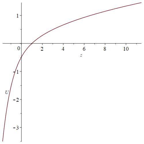
Figure 6: Plot of $U$ against $z$ for the parametric solution (3.83) with $0.505\leq\eta\leq 10$.

Theorem 3.9.

The solutions of the ODE (3.41) for the similarity reduction (3.40) of Novikov’s equation (1.7), with ${\alpha}\neq 0$, are given parametrically by $U=U(Z)$, $z=z(Z)$, where $U$ is defined by

$$U(Z)=\frac{\pm\sqrt{{\alpha}}\,R(Z)}{\sqrt{\genfrac{}{}{}{2}{Z}{3}-R(Z)^{2}}},$$ (3.81)

with $R(Z)$ being a solution of the ODE (3.48), and

$$z(Z)=\tfrac{1}{2}\log\tau_{a+3}(Z)-\tfrac{1}{2}\log\tau_{a}(Z)+\mathrm{const},$$ (3.82)

in terms of two reduced Kaup-Kupershmidt tau functions $\tau_{a}$, $\tau_{a+3}$ connected via the Bäcklund transformation (3.68) for (3.57), and $a=3\big{(}{\alpha}-\genfrac{}{}{}{2}{1}{2}\big{)}$.

• By (3.7), (3.40) and (3.42), we have $U(z)=\pm R(z)/\sqrt{Q(z)}$, so to give the solutions in parametric form we consider $z=z(Z)$ and (by the usual abuse of notation) denote the associated functions with argument $Z$ by the same letters, so that (3.81) follows directly from (3.46) after taking a square root. Then from combining (3.38) and (3.79) we find

  $$\tfrac{1}{2}(v_{+}-v_{-})=\frac{1}{Q}=\tfrac{1}{2}\frac{\mathrm{d}}{\mathrm{d}Z}\left(\log\left(\frac{\hat{\tau}_{a}(Z)^{2}}{\tau_{a}(Z)}\right)-\log\left(\frac{\hat{\tau}_{-a-3}(Z)^{2}}{\tau_{-a-3}(Z)}\right)\right),$$

  and then using (3.80) together with (3.47) this gives

  $$\mathrm{d}z=Q^{-1}\,\mathrm{d}Z=\tfrac{1}{2}\mathrm{d}\,\log\left(\frac{\tau_{a+3}(Z)}{\tau_{a}(Z)}\right),$$

  whence (3.82) follows by integrating, with $a$ fixed in terms of ${\alpha}$ by (3.70). ∎

Example 3.10.

As already mentioned, the ODE (3.57) has a sequence of particular solutions that are algebraic in $Z$, at the parameter values $a=3n$ with $n\in{\mathbb{Z}}$; the first few are presented in Table 2 of [3]. For illustration of the preceding theorem, we consider the simplest of these, which is given by $P=P_{0}(Z)$ with

$$P_{0}=(Z/3)^{1/4},\qquad a=0.$$

Putting this into (3.69) and (3.70) produces a corresponding solution $R=R_{0}(Z)$ of (3.48), where

$$R_{0}=\left(\tfrac{Z}{3}\right)^{-1/4}\left(\Big{(}\tfrac{Z}{3}\Big{)}^{3/4}-\tfrac{1}{4}\right),\qquad{\alpha}=\tfrac{1}{2},$$

which in turn leads to $Q=Q_{0}(Z)$ obtained from (3.46) as

$$Q_{0}=\left(\tfrac{Z}{3}\right)^{-1/2}\left(\Big{(}\tfrac{Z}{3}\Big{)}^{3/4}-\tfrac{1}{8}\right).$$

Upon applying the formula (3.81), we take the plus sign, so that $U=R_{0}/\sqrt{Q_{0}}$; and, rather than computing the tau functions in (3.82), we can directly calculate $z(Z)$ as the integral $z=\int Q_{0}(Z)^{-1}\,\mathrm{d}Z+\,$const. The resulting parametric solution of (3.40) is more conveniently expressed by replacing $Z$ with the parameter $\eta=4(Z/3)^{\genfrac{}{}{}{2}{3}{4}}$, corresponding to the independent variable for Painlevé III, as in (3.62), so that (up to an arbitrary choice of constant in $z$) it takes the form

$$U=\tfrac{1}{\sqrt{2}}\left(\frac{\eta-1}{\sqrt{2\eta-1}}\right),\qquad z=\eta+\tfrac{1}{2}\log(2\eta-1).$$ (3.83)

To check that this agrees with the formula for $z$ in the above theorem, we can use the first two entries in Table 2 of [3] (replacing ${\zeta}\to\eta$ therein), to read off the first two algebraic solutions of (3.57) in terms of $\eta$ as

$$P_{0}=(\eta/4)^{1/3},\qquad P_{3}=(\eta/4)^{1/3}\left(\frac{2\eta-3}{2\eta-1}\right).$$

Then substituting the above into (3.75) for $a=0,3$, and rewriting everything in terms of $\eta$ instead of $Z$, the two reduced Kaup-Kupershmidt fields are found as

$$V_{0}=2^{\genfrac{}{}{}{2}{1}{3}}\eta^{-\genfrac{}{}{}{2}{8}{3}}\Big{(}\tfrac{7}{18}-\tfrac{1}{2}\eta^{2}\Big{)},\qquad V_{3}=-2^{\genfrac{}{}{}{2}{1}{3}}\eta^{-\genfrac{}{}{}{2}{8}{3}}\frac{\Big{(}2\eta^{4}+2\eta^{3}+\tfrac{53}{18}\eta^{2}+\tfrac{14}{9}\eta-\tfrac{7}{18}\Big{)}}{(2\eta-1)^{2}},$$

and then integrating twice with respect to $Z$ and using (3.77), the corresponding tau functions are also written conveniently in terms of the same independent variable for Painlevé III, up to a choice of gauge, as

$$\tau_{0}=\eta^{-\genfrac{}{}{}{2}{7}{36}}\exp\Big{(}-\tfrac{1}{4}\eta^{2}\Big{)},\qquad\tau_{3}=\eta^{-\genfrac{}{}{}{2}{7}{36}}(2\eta-1)\exp\Big{(}-\tfrac{1}{4}\eta^{2}+2\eta\Big{)},$$

so that calculating $\genfrac{}{}{}{2}{1}{2}(\log\tau_{3}-\log\tau_{0})$ from (3.82) indeed reproduces the expression for $z$ in (3.83).

Taking real $\eta>\genfrac{}{}{}{2}{1}{2}$ ensures that $U(z)$ is real-valued. A plot of this solution appears in Fig.6. The behaviour as $\eta$ approaches $\genfrac{}{}{}{2}{1}{2}$ from above is

$$\eta\rightarrow\tfrac{1}{2}+\implies z\to-\infty,\quad U\to-\infty,$$

with leading order asymptotics described by

$$U\sim-\frac{1}{2\sqrt{2}}\,\frac{1}{\sqrt{2\eta-1}},\quad z\sim\tfrac{1}{2}\log(2\eta-1)+\tfrac{1}{2}\implies U\sim-\frac{1}{2\sqrt{2}}\,e^{-\big{(}z-\genfrac{}{}{}{2}{1}{2}\big{)}}.$$ (3.84)

For large $\eta$ the behaviour is

$$\eta\rightarrow\infty\implies z\to\infty,\quad U\to\infty,$$

with leading order asymptotics

$$U\sim\tfrac{1}{2}\sqrt{\eta},\quad z\sim\eta\implies U\sim\tfrac{1}{2}\sqrt{z}.$$

However, the latter does not provide a particularly accurate approximation to the solution. Much greater accuracy can be achieved by reverting the equation for $z$ in (3.83) as $\eta=z-\genfrac{}{}{}{2}{1}{2}\log(2\eta-1)$, using this to generate an expansion

$$\eta=z-\tfrac{1}{2}\log z-\tfrac{1}{2}\log 2+o(1)$$

where the omitted terms above are a double series in powers of $\log(z)$ and $z^{-1}$, and substituting into the formula for $U$ in terms of $\eta$ then gives

$$U\sim\tfrac{1}{2}\sqrt{z}\Big{(}1-\tfrac{1}{4}z^{-1}\log z-\tfrac{1}{4}(3+\log 2)z^{-1}\Big{)},\qquad z\to\infty,$$ (3.85)

omitting terms inside the big brackets above that are $o(z^{-1})$. In Fig.7 we have overlaid plots of the asymptotic approximations (3.84 (blue) and (3.85) (red) on top of part of the plot from Fig.6, which show quite good agreement even for relatively modest magnitudes of $z$ when it is negative/positive, respectively.

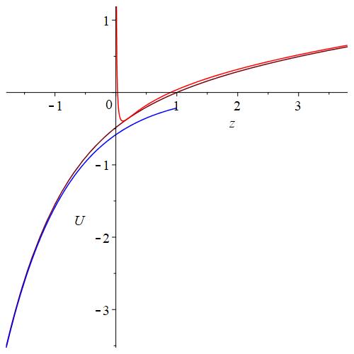
Figure 7: Plot of $U(z)$ compared with asymptotic formulae for the parametric solution (3.83).

In most of our analysis we have made the implicit assumption that ${\alpha}\neq 0$, which was used in the derivation of the ODE (3.48) for $R$. The case ${\alpha}=0$ (separable solutions of Novikov’s equation) corresponds to integrating (3.44) with the integration constant in (3.46) being zero. This implies that $R^{2}-Z/3=0$, which can be regarded as a singular solution of the ODE with ${\alpha}=0$, because both the denominator and the numerator inside the large brackets on the right-hand side of (3.48) vanish. Then $Q(Z)$ satisfies the second order ODE

$$\frac{(Q^{1/2})_{ZZ}}{Q^{1/2}}+\frac{1}{Q^{2}}=-\frac{1}{4Z^{2}}\pm\frac{1}{\sqrt{\tfrac{Z}{3}}},$$ (3.86)

obtained from substituting $R=\pm\sqrt{\genfrac{}{}{}{2}{Z}{3}}$ into the right-hand side of (3.45). The above equation reduces to a Riccati equation for $v$ defined by (3.38), taking $v=v_{+}$ without loss of generality, namely

$$\frac{\mathrm{d}v}{\mathrm{d}Z}-v^{2}=\frac{1}{4Z^{2}}\mp\frac{1}{\sqrt{\tfrac{Z}{3}}},$$ (3.87)

and given the solution $v(Z)$ of the latter, $Q$ is then found from the solution of the inhomogeneous linear equation

$$\tfrac{1}{2}\frac{\mathrm{d}Q}{\mathrm{d}Z}+vQ=1.$$ (3.88)

The other solutions of the ODE with ${\alpha}=0$ are not directly relevant to the scaling similarity solutions of Novikov’s equation, but they have an indirect relevance via the connection to the solutions at parameter values ${\alpha}=3n$ for non-zero integers $n$, corresponding to the solutions of (3.57) for $a=3\big{(}n+\genfrac{}{}{}{2}{1}{2}\big{)}$ that are related to one another by the Bäcklund transformation (3.68).

In order to describe the solutions with ${\alpha}=0$ more explicitly, we set

$$v=-\frac{\mathrm{d}}{\mathrm{d}Z}\log\psi,$$

in the Riccati equation (3.87), which transforms it to the Schrödinger equation

$$\frac{\mathrm{d}^{2}\psi}{\mathrm{d}Z^{2}}+\left(\frac{1}{4Z^{2}}\mp\frac{1}{\sqrt{\tfrac{Z}{3}}}\right)\psi=0.$$ (3.89)

Then, upon changing variables according to

$$\psi(Z)=Z^{\genfrac{}{}{}{2}{1}{2}}\phi(\eta),\qquad\eta=4(Z/3)^{\genfrac{}{}{}{2}{3}{4}},$$

once again using the independent variable $\eta$ for Painlevé III, the equation (3.89) becomes

$$\eta^{2}\frac{\mathrm{d}^{2}\phi}{\mathrm{d}\eta^{2}}+\eta\frac{\mathrm{d}\phi}{\mathrm{d}\eta}\mp\eta^{2}\phi=0,$$

which is solved in terms of Bessel/modified Bessel functions of order 0, depending on the sign. In particular, with the plus sign above, which corresponds to the case $R=-\sqrt{Z/3}$, this implies that the general solution of (3.89) can be written as

$$\psi(Z)=AZ^{1/2}J_{0}\Big{(}4(\tfrac{Z}{3})^{\genfrac{}{}{}{2}{3}{4}}\Big{)}+BZ^{1/2}Y_{0}\Big{(}4(\tfrac{Z}{3})^{\genfrac{}{}{}{2}{3}{4}}\Big{)},$$ (3.90)

for arbitrary constants $A,B$. By replacing $v$ in (3.88) in terms of $\psi$, this reduces to a quadrature for $Q$, namely

$$Q(Z)=2\psi(Z)^{2}\left(\int^{Z}\frac{\mathrm{d}s}{\psi(s)^{2}}+C\right),$$ (3.91)

for another arbitrary constant $C$. (Observe that the formula (3.91) only depends on the ratio $A/B$, so overall this gives two arbitrary constants in the general solution of (3.86), as required.)

For completeness, the case ${\alpha}=0$ is summarized as follows.

Theorem 3.11.

The solutions of the ODE (3.41) with ${\alpha}=0$, which for $z=x$ correspond to the separable solutions (1.10) of Novikov’s equation (1.7), are given parametrically in the form $U=U(Z)$, $z=z(Z)$, with

$$U(Z)=\pm\sqrt{\frac{Z}{3Q(Z)}},\qquad z(Z)=\int^{Z}\frac{\mathrm{d}s}{Q(s)}+\mathrm{const},$$ (3.92)

where $Q(Z)$ is a solution of the ODE (3.86), given by the quadrature (3.91) with $\psi$ specified as in (3.90), or by an analogous formula with modified Bessel functions of order 0.

4 Conclusions

In this paper we have found parametric formulae for the scaling similarity solutions of two integrable peakon equations with cubic nonlinearity, namely (1.1) and (1.7). In both cases, by applying the similarity reduction to suitable reciprocal transformations, and using Miura maps between negative flows of appropriate integrable hierarchies, we have shown that these parametric solutions are related to Painlevé III transcendents, for specific values of the parameters $\tilde{{\alpha}},\tilde{{\beta}},\tilde{{\gamma}},\tilde{\delta}$ in (1.12). More precisely, the scaling similarity solutions of the mCH equation (1.1) are related to the same case of Painlevé III that arises from the Camassa-Holm equation (1.2), while for Novikov’s equation (1.7) such solutions are related to the case of Painlevé III that is associated with an analogous reduction of the Degasperis-Procesi equation (1.9).

The scaling similarity solutions of the mCH equation (1.1) have been written parametrically in terms of solutions of the ODE (2.52), which is of second order and second degree. The systematic study of such equations was initiated in [10], although to the best of our knowledge there is still no complete classification of second order, second degree equations with the Painlevé property. Certain particular equations of this type, the so-called sigma forms of the Painlevé equations, which are the equations satisfied by Okamoto’s Hamiltonians [34], play an important role in both theory and applications. However, the ODE (2.52) is of a different kind, since the Hamiltonians are quadratic functions of the first derivatives of the solution of the corresponding Painlevé equation, whereas the transformation (2.64) is linear in $\genfrac{}{}{}{2}{\mathrm{d}P}{\mathrm{d}Z}$, with $P(Z)$ being a solution of Painlevé III.

For the case of Novikov’s equation (1.7), the scaling similarity solutions are expressed parametrically in terms of solutions of the ODE (3.48), which is equivalent to the Painlevé V equation with a particular choice of parameters, and arises via reduction of the negative Sawada-Kotera flow (3.10). The equation (3.48) has a one-to-one correspondence with the ODE (3.57) obtained via the scaling similarity reduction for the negative Kaup-Kupershmidt flow (3.6), which in turn is equivalent to another particular case of Painlevé III. The correspondences and Bäcklund transformations between the solutions of (3.57) and (3.48) have been constructed using properties of these solutions that are naturally inherited from the two Miura maps in (3.3), which relate the Kaup-Kupershmidt and Sawada-Kotera PDE hierarchies to the same underlying modified hierarchy. However, implicit in our construction is the fact that there is a negative flow in the latter hierarchy, which should be given by a PDE of third order for the modified field $v=v(X,T)$, while at the level of the scaling similarity reductions there must be an ODE of second order for the reduced variable $v(Z)$. It has not been necessary to write them down here, but computer algebra calculations show that these equations are somewhat unwieldy: the modified PDE for $v(X,T)$ is of second degree in the highest derivative that appears, namely $v_{XXT}$, while the reduced ODE for $v(Z)$ is of third degree in its second derivative $v_{ZZ}$, so we have thought it best to leave a more detailed discussion of these matters for elsewhere.

Acknowledgments: LEB was supported by a PhD studentship from SMSAS, Kent. The research of ANWH was funded in 2014-2021 by Fellowship EP/M004333/1 from the Engineering & Physical Sciences Research Council, UK, with a UKRI COVID-19 Grant Extension, and is currently supported by grant IEC\R3\193024 from the Royal Society. The inception of this research project was made possible thanks to support from the Royal Society and the Department of Science & Technology (India) going back to 2005, which allowed Senthilvelan to visit Hone under the India-UK Science Network and Scientific Seminar schemes. Conflict of Interest: The authors declare that they have no conflicts of interest.

References

- [1] M.J. Ablowitz, A. Ramani and H. Segur. Lettere al Nuovo Cimento 23 (1978) 333–338.
- [2] L.E. Barnes. Integrable and non-integrable equations with peaked soliton solutions. PhD thesis, University of Kent, 2020.
- [3] L.E. Barnes and A.N.W. Hone, Theor. Math. Phys. (2022), at press; arXiv:2201.00265
- [4] A.P. Bassom, P.A. Clarkson and A.E. Milne, Stud. Appl. Math. 98 (1997) 139–194.
- [5] R. Camassa and D.D. Holm. Phys. Rev. Lett. 71 (1993) 1661–4.
- [6] R. Camassa, D.D. Holm and J.M. Hyman. Advances in Applied Mechanics 31 (1994) 1–33.
- [7] X.K. Chang and J. Szmigielski. J. Nonlinear Math. Phys. 23 (2016) 563–72.
- [8] P.A. Clarkson, J. Phys. A: Math. Gen. 36 (2003) 9507.
- [9] A. Constantin and D. Lannes. Archive for Rational Mechanics and Analysis 192 (2009) 165–186.
- [10] C.M. Cosgrove and G. Scoufis. Stud. Appl. Math. 88 (1993) 25–87.
- [11] A. Degasperis, D.D. Holm and A.N.W. Hone. Theor. Math. Phys. 133 (2002) 1461–72.
- [12] A. Degasperis and M. Procesi. Asymptotic integrability. Symmetry and Perturbation Theory, eds. A. Degasperis and G. Gaeta. World Scientific (1999) pp. 23–37.
- [13] B. Dubrovin, T.Grava and C. Klein. J. Nonlinear Sci. 19 (2009) 57–94.
- [14] H.R. Dullin, G.A. Gottwald and D.D. Holm. Fluid Dynamics Research 33 (2003) 73–95.
- [15] H.R. Dullin, G.A. Gottwald and D.D. Holm. Physica D 190 (2004) 1–14
- [16] H. Flaschka and A.C. Newell. Commun. Math. Phys. 76 (1980) 65–116.
- [17] A.S. Fokas and B. Fuchssteiner. Physica D 4 (1981) 47–66.
- [18] A.S. Fokas. Physica D 87 (1995) 145–150.
- [19] A.P. Fordy and J. Gibbons. J. Math. Phys. 21 (1980) 2508–2510.
- [20] C. Gilson and A. Pickering. J. Phys. A: Math. Gen. 28 (1995) 2871.
- [21] P.R. Gordoa and A. Pickering. J. Math. Phys. 40 (1999) 5749.
- [22] V.I. Gromak. Differ. Uravn. 11 (1975) 373–376 (Russian).
- [23] G.L. Gui, Y. Liu, P.J. Olver and C.Z. Qu. Commun. Math. Phys. 319 (2013) 731–59.
- [24] D.D. Holm and M. Staley, Phys. Lett. A 308 (2003) 437–444.
- [25] A.N.W. Hone. J. Phys. A 32 (1999) L307–L314
- [26] A.N.W. Hone. Painlevé Tests, Singularity Structure and Integrability. Integrability, ed. A.V. Mikhailov. Lect. Notes Phys. 767, Springer, Berlin, Heidelberg (2009) pp. 245–277.
- [27] A.N.W. Hone and J.P. Wang. Inverse Problems 19 (2003) 129–145.
- [28] A.N.W. Hone and J.P. Wang. J. Phys. A: Math. Theor. 41 (2008) 372002.
- [29] R.I. Ivanov. Phil. Trans. R. Soc. A 365 (2007) 2267–2280.
- [30] Y.A. Li and P.J. Olver. Discrete & Continuous Dynamical Systems 3 (1997) 419–432.
- [31] H. Lundmark and J. Szmigielski. arXiv:2203.12954v1
- [32] A.V. Mikhailov and V.S. Novikov. J. Phys. A: Math. Gen. 35 (2002) 4775–90.
- [33] V. Novikov. J. Phys. A: Math. Theor. 42 (2009) 342002.
- [34] K. Okamoto. Physica D 2 (1981) 525–535.
- [35] P.J. Olver and P. Rosenau. Phys. Rev. E 53 (1996) 1900–1906.
- [36] NIST Digital Library of Mathematical Functions. http://dlmf.nist.gov/, Release 1.1.5 of 2022-03-15. F.W.J. Olver, A.B. Olde Daalhuis, D.W. Lozier, B.I. Schneider, R.F. Boisvert, C.W. Clark, B.R. Miller, B.V. Saunders, H.S. Cohl, and M.A. McClain, eds.
- [37] A. Pickering. Theor. Math. Phys. 135 (2003) 638–641.
- [38] Z. Qiao. J. Math. Phys. 47 (2006) 112701–9.
- [39] J. Schiff. Physica D 121 (1998) 24–43.
- [40] S. Stalin and M. Senthilvelan. Phys. Lett. A 375 (2011) 3786–3788.
- [41] G. Wang, Q.P. Liu and H. Mao. J. Phys. A: Math. Theor. 53 (2020) 294003.