Scalable almost-linear dynamical Ising machines

Abstract

The past decade has seen the emergence of Ising machines targeting hard combinatorial optimization problems by minimizing the Ising Hamiltonian with spins represented by continuous dynamical variables. However, capabilities of these machines at larger scales are yet to be fully explored. We investigate an Ising machine based on a network of almost-linearly coupled analog spins. We show that such networks leverage the computational resource similar to that of the semidefinite positive relaxation of the Ising model. We estimate the expected performance of the almost-linear machine and benchmark it on a set of $\left\{0,1\right\}$-weighted graphs. We show that the running time of the investigated machine scales polynomially (linearly with the number of edges in the connectivity graph). As an example of the physical realization of the machine, we present a CMOS-compatible implementation comprising an array of vertices efficiently storing the continuous spins on charged capacitors and communicating externally via analog current.

1 Introduction

Many existing practical optimization problems such as resource allocation, traffic control, cell placement and interconnection routing within in a very large-scale integrated (VLSI) chip, as well as emerging problems like polymer modelling Babbush2014ConstructionAnnealing , protein folding Fraenkel1993ComplexityFolding and medical image segmenting ref_imag are NP hard, that is, as the problem scales in size, they require exponentially more computing resources to obtain an exact solution. As the growth of the problem size outpaces scaling of commercial processors, alternative faster computing techniques are being actively sought.

One such alternative is based on classical spin systems on graphs. The computational significance of these systems lies in a tight connection between the distribution of spins delivering the lowest energy and the maximal cut of the graph barahona_computational_1982 . In turn, the maximal cut problem is NP-complete miller_reducibility_1972 ; gareySimplified1976 and therefore finding the ground state of the Ising model can be employed for solving other NP-hard problems. This principle was explicated in Lucas2014IsingProblems , where it was shown that all Karp’s original NP-complete problems can be solved by finding the ground state of Ising models with specially crafted Hamiltonians.

The computational capabilities of spin systems are known for several decades. Based on analogy with the thermal relaxation to the ground state, a well-known class of algorithms with wide area of applications, simulated annealing, was invented in Kirkpatrick1983OptimizationAnnealing . The success of simulated annealing motivated several digital annealing processors Yamaoka201520k-spinAnnealing ; Takemoto2020AProblems ; su312020 ; takemoto144Kb2021 ; okuyamaComputing2016 ; Yamamoto2017AFPGAs , which utilized the direct analogy between binary states of classical spins in the Ising model and binary devices. To emulate the thermal effect helping to traverse the configuration space of the spin system, randomized spin-flips were implemented using on-chip random bit-sequence generators.

Recently, a new generation of Ising machines based on continuous dynamics has emerged Ahmed2021AProblems ; Bashar2020ExperimentalProblem ; Parihar2017VertexNetworks ; Raychowdhury2019ComputingSystems ; Marandi2014NetworkMachine ; McMahon2016AConnections ; Bohm2019AProblems ; Leleu2017CombinatorialSystems ; Molnar2018APerformance ; afoakwaBRIM2021 . These machines do not attempt to represent the binary states of the classical spin. Instead, they leverage the emergent capability of selected dynamical systems to deliver the ground state of the Ising Hamiltonian.

The continuous dynamical Ising machines are demonstrated the ability to achieve good quality solutions on benchmark problems, such as GSet gset . At the same time, the problem of scaling of the computational budget, for instance, running time, drew much less attention. The scaling problem is important in the context of NP-complete problem, especially considering the APX-hardness of the max-cut problem papadimitriou_optimization_1991 ; khot_optimal_2004 . This means that the approximation achievable in time scaling polynomially with the problem size is limited if $\mathrm{P}\neq\mathrm{NP}$. The existing data on scaling of dynamical Ising machines hamerlyExperimental2019 ; leleuScaling2021a demonstrate super-polynomial scaling: the best result reported in leleuScaling2021a is $\mathcal{O}\left(e^{\sqrt{N}}\right)$, where $N$ is the number of graph nodes. Such scaling effectively puts large NP-hard problem out of the reach.

In erementchoukComputational2022 , we have shown that Ising machines based on oscillator networks realizing the Kuramoto model of synchronization can demonstrate the polynomial scaling, while delivering solutions of good quality. This is related to the fact that the equations of motion of the Kuramoto model in the synchronized regime implement the gradient-descent solution of the rank-2 semidefinite programming relaxation. It should be noted in this regard that large scale physical realizations of Ising machines must resolve fundamental challenges associated with the high degree of integration. The dynamical model governing the Ising machine must be simple enough to admit a straightforward realization and robust to withstand unavoidable imperfections and variations. At the same time, this must be achieved without sacrificing computational capabilities.

In this work, we investigate an approach of realizing dynamical Ising machines that overcomes the challenges associated with oscillatory systems while retaining their computational capabilities. We consider an almost-linear dissipative dynamical system on a graph. We show that this model presents an approximation of the rank-$2$ semidefinite positive (SDP) relaxation of the Ising model. As a result, the model is capable of providing a good approximation in time, which scales polynomially with the number of edges. We show that the machine is characterized by the integrality gap close to that of the SDP relaxation and demonstrates the core performance comparable with the state-of-the-art solves.

As a proof-of-concept, we present a CMOS-compatible combinatorial optimizer that implements the investigated almost-linear Ising machine. The analog-digital mixed mode computing system is based on fully integrated components using a 130 nm CMOS technology.

This paper is organized as follows. In Section 2, we present the necessary theoretical background and find the integrality gap of the almost-linear Ising machine. In Section 3, we consider a software simulation of the machine, and investigate its performance on benchmark tests and its scaling properties. In Section 4, we describe the CMOS computing system implementing the almost-linear dynamical Ising machine.

2 Dynamical Ising machines

2.1 Ising model and NP-hard problems

Let $\mathcal{G}=\{\mathcal{V},\mathcal{E}\}$ be a graph with $N$ vertices and $M$ edges given by sets $\mathcal{V}$ and $\mathcal{E}$, respectively. The Ising model on $\mathcal{G}$ deals with binary (taking values $\pm 1$) functions on the set of graph vertices, $\boldsymbol{\sigma}:\mathcal{V}\to\{-1,1\}$. Alternatively, such functions can be understood as assigning a binary variable $\sigma_{i}$ to the $i$-th vertex resulting in configuration $\boldsymbol{\sigma}=\{\sigma_{i}\}$. The sets of nodes where $\boldsymbol{\sigma}$ takes positive and negative values define partitioning of the graph nodes $\mathcal{V}=\mathcal{V}_{+}\cup\mathcal{V}_{-}$. Finding the partitioning with the maximal number of edges connecting nodes in $\mathcal{V}_{+}$ and $\mathcal{V}_{-}$ is the maximal cut problem. This problem is NP-complete miller_reducibility_1972 ; gareySimplified1976 and, therefore, finding its solution provides ways to solve other NP-complete problems Lucas2014IsingProblems .

The Ising model is defined by assigning the energy to configurations

$${H}_{I}(\boldsymbol{\sigma})=\frac{1}{2}\sum_{m,n=1}^{N}A_{m,n}\sigma_{m}\sigma_{n},$$ (1)

where $A_{m,n}$ is the graph adjacency matrix. It is straightforward to show that finding the ground state ($\boldsymbol{\sigma}$ yielding the lowest ${H}_{I}(\boldsymbol{\sigma})$) of the Ising model is equivalent to solving the max-cut problem barahona_computational_1982 . The function taking values $1$ on edges connecting $\mathcal{V}_{+}$ and $\mathcal{V}_{-}$ and $0$ elsewhere can be written in terms of $\boldsymbol{\sigma}$ as $(1-\sigma_{m}\sigma_{n})/2$. Thus, the total number of cut edges is

$$C_{\mathcal{G}}\left(\boldsymbol{\sigma}\right)=\frac{1}{4}\sum_{m,n}A_{m,n}\left(1-\sigma_{m}\sigma_{n}\right)=\frac{M}{2}-\frac{1}{2}{H}_{I}\left(\boldsymbol{\sigma}\right).$$ (2)

2.2 Ising machines based on the Kuramoto model

The operational principles of the presented architecture are based on a proper adaptation of the principles enabling Ising machines based on synchronizing oscillator networks. Therefore, we first review the computational capabilities of such machines, and then we abstract them from the oscillatory dynamics to formulate the dynamical model of our main interest.

The Kuramoto model was originally introduced to study the synchronization phenomenon in networks with inhomogeneous natural frequencies. However, in the computing context, where the informational content is associated with relative phases of the oscillators, the frequency variation can be expected to play a detrimental role. Therefore, we consider a network of oscillators with identical natural frequencies. In this case, the relative phases obey the equations of motion

$$\frac{1}{K}\dot{\theta}_{m}=\sum_{n}A_{m,n}\sin(\theta_{n}-\theta_{m})+\frac{\widetilde{K}_{s}}{K}\sin(2\theta_{m}).$$ (3)

Here, $\theta$ is the phase of the $m$-th oscillator in the rotating frame (with subtracted common linear in time contribution), $K$ is the coupling parameter, matrix $\widehat{A}$ with matrix elements $A_{m,n}$ is the network adjacency matrix, and $\widetilde{K}_{s}$ is the strength of the phase injection adler_StudyLocking_1946 ; bhansaliGenAdler2009 . By rescaling time, one can always choose $K=1$. Since the analysis below does not depend on the time scale, we simplify formulas by denoting $K_{s}=\widetilde{K}_{s}/K$ and taking $K=1$.

The equations of motion can be presented as induced by the Lyapunov function

$$H_{K}=\frac{1}{2}\sum_{m,n}A_{m,n}\cos(\theta_{m}-\theta_{n})-\frac{K_{s}}{2}\sum_{m}\cos^{2}(\theta_{m}).$$ (4)

Indeed, one can see that $\dot{\theta}_{m}=-\partial H_{K}/\partial\theta_{m}$, implying that $dH_{K}/dt\leq 0$. Thus, the system evolves in such a way that $H_{K}$ monotonously decreases, unless the system is in an equilibrium state, where $\dot{\theta}_{m}=0$.

The extremal spectral properties of the Kuramoto model, the global minimum of $H_{K}$ and the minimizing configurations, are tightly related to the extremal properties of the Ising Hamiltonian $H_{I}$. This is the relation between an integer program and its relaxations, as identified in the theory of combinatorial optimization. To make this connection more straightforward, we will consider it from the perspective of the max-cut problem.

First, we observe that $H_{K}$ is equivalent to the Hamiltonian of the $XY$ model, which deals with unit vector distributions given by functions $\mathbf{s}:\mathcal{V}\to\mathbb{S}^{1}$, where $\mathbb{S}^{1}$ is the set of unit 2D vectors:

$$H^{(XY)}(\mathbf{s})=\frac{1}{2}\sum_{m.n}A_{m,n}\vec{s}_{m}\cdot\vec{s}_{n}-\frac{1}{2}\sum_{m}{\left(\vec{l}\cdot\vec{s}_{m}\right)}^{2},$$ (5)

where $\vec{s}_{m}$ are unit vectors confined to a 2D plane, and $\vec{l}$ is the anisotropy axis. Defining the orientation of $\vec{s}_{m}$ in terms of angle $\theta_{m}$ with respect to $\vec{l}$, so that we can write $\vec{s}_{m}={\left(\cos(\theta_{m}),\sin(\theta_{m})\right)}^{T}$ in (5), we obtain (3).

Representing $H^{(K)}$ as a Hamiltonian of the XY model reveals the connection between the dynamics of the Ising machine based on the synchronizing oscillator network and the Ising model. The max-cut problem can be presented as an integer program korte_CombinatorialOptimization_2018

$$\overline{C}_{\mathcal{G}}=\max_{\Xi}\left[\frac{M}{2}-\frac{1}{4}\mathrm{Tr}\left(\widehat{A}\widehat{\Xi}\right)\right],$$ (6)

where matrix $\widehat{\Xi}$ is subject to constraints $\Xi_{i,i}=1$ and $\mathrm{rank}(\widehat{\Xi})=1$. It is easy to check that $\widehat{\Xi}$ satisfies these constraints if and only if $\Xi_{i,j}=\sigma_{i}\sigma_{j}$ with binary $\sigma_{i}$. Thus, (6) is equivalent to the original formulation.

Let $C_{\mathcal{G}}^{(XY)}(\mathbf{s})=M/2-H^{(XY)}(\mathbf{s})/2$ be a formal analog of cut for the XY model defined by using $H^{(XY)}$ instead of the Ising Hamiltonian in Eq. (2) or, equivalently, by using $\widehat{\Xi}^{(XY)}$ with $\Xi_{i,j}^{(XY)}=\vec{s}_{i}\cdot\vec{s}_{j}$ instead of $\widehat{\Xi}$. One can see that the maximal value of $C_{\mathcal{G}}^{(XY)}$ is found by solving Eq. (6) with the relaxed rank constraint, $\mathrm{rank}(\widehat{\Xi})=2$, and requirement that $\widehat{\Xi}^{(XY)}$ is positive semidefinite. Thus, the isotropic XY model, and, hence, the isotropic Kuramoto model implement the rank-$2$ semidefinite programming (SDP) relaxation of the max-cut problem goemans_ImprovedApproximation_1995 ; alon_BipartiteSubgraphs_2000 ; deza_GeometryCuts_1997 ; Burer2002Rank-twoPrograms .

One of the key elements of SDP relaxations is obtaining the binary state of the Ising model, since finding the solution of the SDP relaxation does not reduce the complexity of the max-cut problem laurent_positive_1995 . Let the relaxed problem be solved by configuration $\mathbf{s}^{(0)}$ yielding $\overline{\mathcal{C}}_{\mathcal{G}}^{(XY)}=C_{\mathcal{G}}^{(XY)}\left(\mathbf{s}^{(0)}\right)$. Generally, vectors $\vec{s}^{(0)}_{i}$ are not oriented along the same line, and, to reconstruct an Ising configuration, the XY configuration must be rounded. This can be done by choosing unit vector $\vec{t}$ and mapping vectors $\vec{s}^{(0)}_{i}$ to $\left\{-1,1\right\}$ according to $\sigma_{i}\left(\vec{t}\right)=\mathrm{sign}\left(\vec{s}^{(0)}_{i}\cdot\vec{t}\right)$, as illustrated by Fig. 1(a).

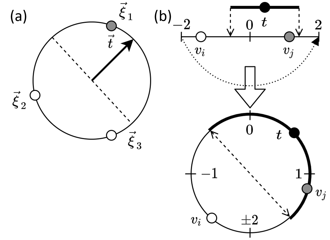
Figure 1: The rounding rules. (a) The rank-$2$ relaxation: vectors making positive dot product with $\vec{t}$ are rounded to $1$ ($\vec{\xi}_{1}$, filled circles), and the rest are rounded to $-1$ ($\vec{\xi}_{2}$ and $\vec{\xi}_{3}$, hollow circles). (b) The triangular model: the rounding center $t$ defines the center of the interval for mapping to $1$ ($v_{j}$ shaded circle), the rest of the variables are mapped to $-1$.

Averaging obtained cut over orientations of $\vec{t}$ yields goemans_ImprovedApproximation_1995

$$\left\langle C_{\mathcal{G}}\left(\boldsymbol{\sigma}(\vec{t})\right)\right\rangle_{\vec{t}}\geq\alpha_{\text{G-W}}\overline{C}_{\mathcal{G}},$$ (7)

where $\alpha_{\text{G-W}}=\min_{\theta>0}\frac{\theta}{\pi\sin^{2}(\theta/2)}\approx 0.877\ldots$.

Inequality (7) guarantees that rounding the found solution of the relaxed problem yields the cut at least within $13\%$ of the maximal cut. This is the best, assuming that $\mathrm{P}\neq\mathrm{NP}$, performance of an approximation to the max-cut problem running in polynomial time.

Taking into account that $\mathcal{C}_{\mathcal{G}}\left(\boldsymbol{\sigma}(\vec{t})\right)$ cannot exceed the maximum cut, we obtain an important inequality estimating the integrality gap, the mismatch between the solutions of the relaxed and the original problems:

$$\overline{C}_{\mathcal{G}}\geq\alpha C_{\mathcal{G}}^{(XY)}\left(\mathbf{s}^{(0)}\right).$$ (8)

Equations (7)–(8) remain valid for arbitrary non-negatively weighted adjacency matrices. The case, when both, positive and negative, weights are allowed, is more complex. However, the performance ratio and the integrality gap can be estimated in this case as well charikar_MaximizingQuadratic_2004 ; alon_ApproximatingCutnorm_2004 ; anjos_StrengthenedSemidefinite_2002 .

This consideration explains why dynamic Ising machines based on the Kuramoto model can solve the max-cut problem and indicates that such machines solvers can be quantitatively described by the target performance guarantee. This is important because dynamical Ising machines that do not converge to the Kuramoto model may leverage different computational resources. Correctly identifying the origin of the computational power allows recognizing the best area of applications, potential weaknesses and challenges, and how to address them.

We conclude by noting that the gradient descent, generally, does not reach the global minimum of $H^{(XY)}$ Burer2002Rank-twoPrograms ; erementchoukComputational2022 . At present, the common approach to address this problem is to rerun the machine multiple times. Alternative strategies for improving convergence can be explored but are beyond the scope of the present paper.

2.3 Almost-linear Ising machine

The consideration above shows the natural connection between the SDP relaxation and the dynamics of coupled phase oscillators with linear coupling. Once the origin of the computational capabilities of oscillatory IMs is established, one may reproduce it in a non-oscillatory dynamical environment.

We consider an approach utilizing continuous unbounded dynamical variables, which, for instance, can be represented by the electric charge. To make such system behaving similarly to the XY model (and, hence, reproducing SDP relaxations), one needs to emulate a cosine-like coupling between individual variables. In the present paper, we avoid implementing such a costly emulation by departing from the SDP approach in favor of a significantly simplified model of coupling between the dynamical variables.

In the present paper, we explore a piece-wise linear approximation of the coupling and the anisotropy functions in Eq. (3). Using the same conventions, $K_{s}=\widetilde{K}_{s}/K$ and $K=1$, the general equations of motion are of the form

$$\dot{v}_{i}=-\sum_{j}A_{i,j}\phi(v_{i}-v_{j})+K_{s}\phi(2v_{i}),$$ (9)

where $v_{i}$ are dynamical variables with unrestricted values. The coupling function, $\phi(v)$, is a piece-wise linear periodic function consistent with a relaxation of the max-cut problem. We will slightly reduce the generality of our consideration by requiring that $\phi(v)$ is an odd function.

To find $\phi(v)$, we consider the equations of motion as induced by the Lyapunov function

$$H^{(\Phi)}(\mathbf{v})=\frac{1}{2}\sum_{i,j}A_{i,j}\Phi(v_{i}-v_{j})-\frac{K_{s}}{2}\sum_{i}\Phi(2v_{i}),$$ (10)

where $\Phi(v)$ is an even periodic function related to the coupling function by $d\Phi(v)/dv=\phi(v)$, and satisfying $\Phi(0)=1$ and $\Phi(\pm 2)=-1$.

Next, we define

$$C_{\mathcal{G}}^{(\Phi)}\left(\mathbf{v}\right)=\frac{M}{2}-\frac{1}{4}\mathrm{Tr}\left(\widehat{A}\widehat{\Xi}^{(\Phi)}\right),$$ (11)

where ${\Xi}^{(\Phi)}_{i,j}=\Phi(v_{i}-v_{j})$. On feasible ($v_{i}=\pm 1$) Ising configurations, $C_{\mathcal{G}}^{(\Phi)}$ coincides with the cut. Thus, the problem

$$\overline{C}_{\mathcal{G}}^{(\Phi)}=\max_{\mathbf{v}}C_{\mathcal{G}}^{(\Phi)}\left(\mathbf{v}\right)$$ (12)

is a proper relaxation of the max-cut problem and $\overline{C}_{\mathcal{G}}^{(\Phi)}\geq\overline{C}_{\mathcal{G}}$.

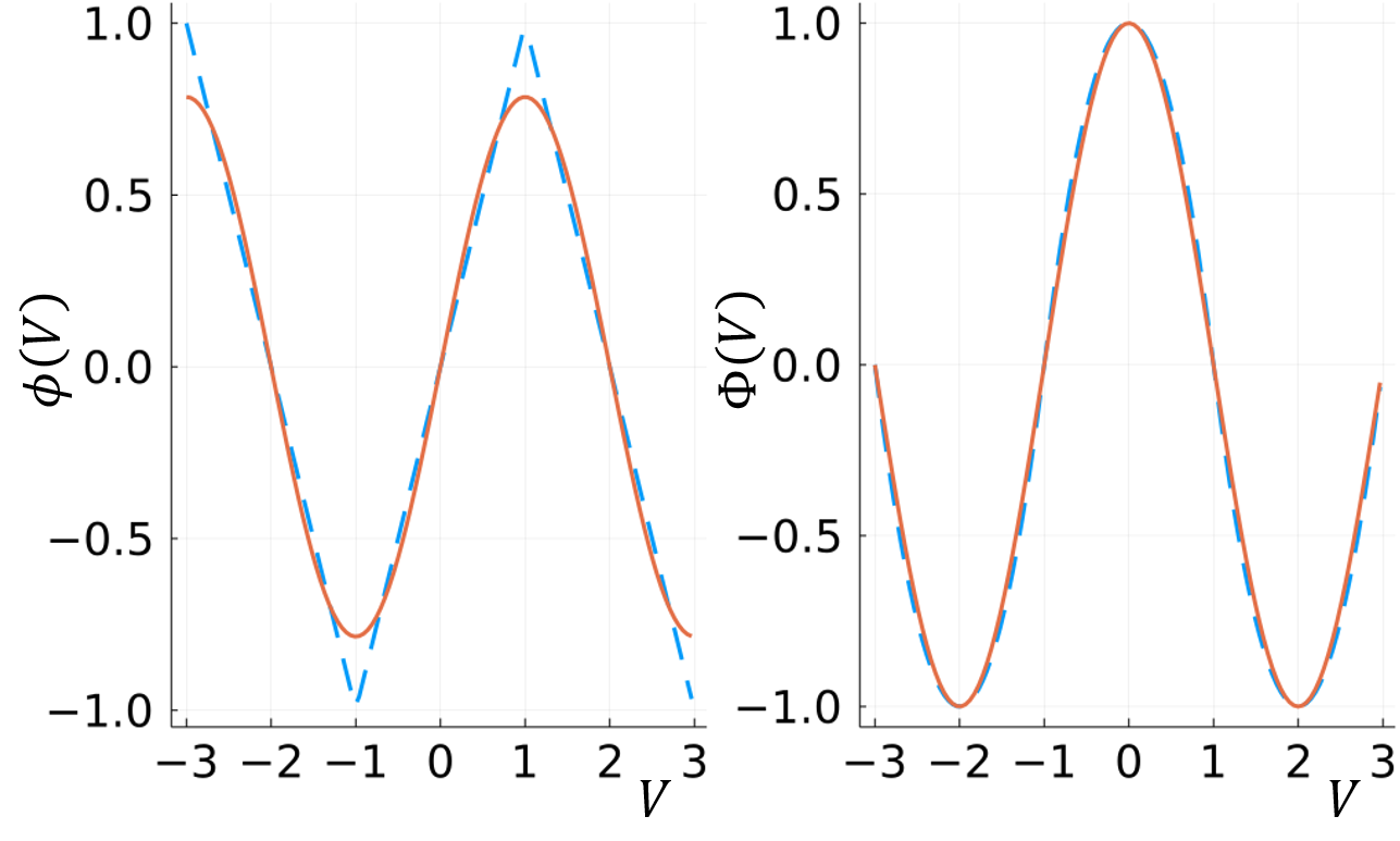
Figure 2: Comparison of the dynamic coupling function $\phi(v)$ and the Hamiltonian kernel $\Phi(v)$ for the rank-2 relaxation (solid line) and the triangular model (dashed line)

The simplest form of continuous with its derivative $\Phi(v)$ yielding a piece-wise linear $\phi(v)$ is a function with the period $P=4$ and defined within one period by

$$\Phi(v)=\begin{cases}1-v^{2},&-1\leq v\leq 1,\\ {(v-2)}^{2}-1,&1\leq v\leq 3.\end{cases}$$ (13)

This corresponds to

$$\phi(v)=2\begin{cases}-v,&-1\leq v\leq 1,\\ v-2,&1\leq v\leq 3.\end{cases}$$ (14)

We will call this relaxation the triangular model. Figures 1(c,d) compare the coupling functions of the XY and the triangular models showing the relationship between them.

The rounding procedure for the triangular model can be defined as follows. Let $\mathbf{v}^{(0)}$ be a maximizing configuration so that $\overline{C}_{\mathcal{G}}^{(\Phi)}=C_{\mathcal{G}}^{(\Phi)}\left(\mathbf{v}^{(0)}\right)$. Because of the periodicity of $\Phi(v)$, we can take $v_{i}^{(0)}$ modulo $P$ and restrict them to the single period, say, $\left[-2,2\right]$, with identified ends. Such mapping of $v_{i}^{(0)}$ makes the rounding procedure for the triangular model essentially the same as for the XY model as illustrated by Fig. 1(a). For the chosen rounding center $t$, those $v_{i}$ that fall inside the interval $\left[t-P/2,t+P/2\right)$ are mapped to $+1$, while the rest are mapped to $-1$. We denote the rounding mapping for the given rounding center $t$ by $\boldsymbol{\sigma}=\widehat{R}\left[\mathbf{v}^{(0)}\mathchar 24635\relax\;t\right]$.

Moreover, the performance and the integrality gap can also be estimated using the same argument as for the SDP relaxations. Let $\boldsymbol{\sigma}(t)$ is the Ising configuration obtained by mapping $\mathbf{v}^{(0)}$ to $\left\{-1,1\right\}^{N}$ with the given the rounding center $t$. Averaging the resultant cut over the random choices of $t$, we find

$$\left\langle C_{\mathcal{G}}\left(\boldsymbol{\sigma}(t)\right)\right\rangle_{t}=\sum_{i,j}A_{i,j}\mathcal{P}\left(v_{i}^{(0)},v_{j}^{(0)}\right),$$ (15)

where $\mathcal{P}\left(v_{i}^{(0)},v_{j}^{(0)}\right)$ is the probability that $v_{i}^{(0)}$ and $v_{j}^{(0)}$ fall into different intervals and, hence, edge $(i,j)$ contributes to the cut. Because of the rotational symmetry of the rounding, this probability may depend only on the mutual arrangement of $v_{i}^{(0)}$ and $v_{j}^{(0)}$. Thus, we have the usual geometric probability situation and can write

$$\mathcal{P}\left(v_{i}^{(0)},v_{j}^{(0)}\right)=\frac{2}{P}\left|v_{i}^{(0)}-v_{j}^{(0)}\right|_{P},$$ (16)

where $\left|v_{i}^{(0)}-v_{j}^{(0)}\right|_{P}$ is the distance between $v_{i}^{(0)}$ and $v_{j}^{(0)}$ along the circumference in Fig. 1(a) (the length of the shortest path).

Thus, we have

$$\begin{split}\left\langle C_{\mathcal{G}}\left(\boldsymbol{\sigma}(t)\right)\right\rangle_{t}&=\sum_{i,j}A_{i,j}\frac{2}{P}|v_{i}^{(0)}-v_{j}^{(0)}|_{P}\\ &\geq\alpha_{T}\sum_{i,j}A_{i,j}\frac{1}{2}\left[1-\Phi\left(v_{i}^{(0)}-v_{j}^{(0)}\right)\right]\\ &\geq\alpha_{T}\overline{C}_{\mathcal{G}}^{(\Phi)}\geq\alpha_{T}\overline{C}_{\mathcal{G}},\end{split}$$ (17)

where

$$\alpha_{T}=\frac{4}{P}\min_{|v|\leq 2}\frac{|v|}{1-\Phi(v)}\approx\frac{4}{P}0.85\ldots.$$ (18)

This estimates the integrality gap of the triangular model and its enabling max-cut performance.

Above, we kept explicitly period $P$ of the coupling function to show that $P=4$ is, in a sense, optimal. Such an optimization, of course, is trivial from the perspective of various nonlinear relaxations. Even when restricted to translationally invariant $\Phi(v)$ yielding piece-wise linear $\phi(v)$, the family of these relaxations is very rich from the perspective of enabled dynamics and performance consequences. The respective family of dynamical Ising machines based on different coupling functions $\Phi(v,v^{\prime})$ is yet to be explored. In the present paper, we limit ourselves to the triangular model as a particular representative of the extended family.

3 Software simulation of the almost-linear Ising machine

In this section, we present the software simulation of the Ising machine based on the triangular model. It should be noted that there are various ways of improving the practical performance of the Ising machine. For example, the adaptive dynamics can be used for speeding up the convergence of the machine to a steady state, restarting the machine from a slight perturbation of the previously found the best configuration and special schedules for time varying anisotropy constant, $K_{s}$, can improve the search for more optimal solutions, and so on. A detailed analysis of such techniques, however, is beyond the scope of the present paper, and we focus on studying the core performance of the Ising machine based on the triangular model.

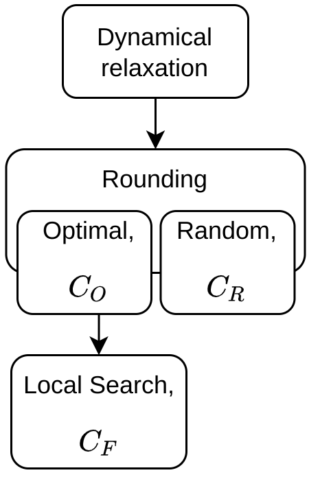
Figure 3: Three setups testing the basic performance of the Ising machine based on the triangular model

The general structure of simulations is shown in Fig. 3. Testing consists of three stages. During the first stage, the Ising machine evolves freely according to the equations of motion solved using the Euler approximation. During the second stage, the machine state established after the fixed number of time steps is rounded to construct a binary state of the Ising model. As has been discussed above, rounding is one of the key elements of finding the maximal cut using the SDP relaxation. Therefore, we compare two approaches to rounding based on mapping $\widehat{R}$ defined above.

One approach leverages the observation that averaging cut over randomly chosen rounding centers is sufficient for getting the best performance assuming that $\text{P}\neq\text{NP}$ khot_optimal_2004 . Within this approach, the rounding center is sampled $n_{R}$ times from the uniform distribution over the interval $\left[-1,1\right]$. The configuration is rounded according to the chosen values of the rounding center and the best value of cut out of $n_{R}$ is kept.

procedure Random-Rounding(input $\mathcal{G}$, $\mathbf{v}$, $n_{R}$; output $C_{R}$, $\boldsymbol{\sigma}_{R}$)

     $C_{R}\leftarrow-1$

     Let $\left\{t_{1},\ldots,t_{n_{R}}\right\}$ be a sample of the uniform distribution on $\left[-1,1\right]$

     for all $t_{i}\in\left\{t_{1},\dots,t_{n_{R}}\right\}$ do

         $\boldsymbol{\sigma}(t_{i})\leftarrow\widehat{R}[\mathbf{v}\mathchar 24635\relax\;t_{i}]$

         $C(t_{i})\leftarrow C_{\mathcal{G}}\left(\boldsymbol{\sigma}(t_{i})\right)$

         if $C(t_{i})>C_{R}$ then

              $C_{R}\leftarrow C(t_{i})$

              $\boldsymbol{\sigma}_{R}\leftarrow\boldsymbol{\sigma}(t_{i})$

         end if

     end for

end procedure

The second approach evaluates all non-equivalent binary states that can be obtained by varying the rounding center. This can be achieved by monotonously traversing the interval $[-1,1)$. Ordering coinciding $v^{(0)}_{i}$ according to the nodes enumeration, one can ensure that the recovered partitions change by a single node as illustrated by Fig. 4.

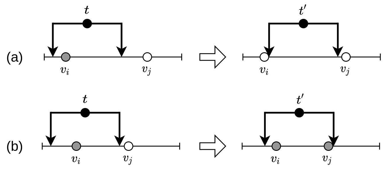
Figure 4: The rounding center can be shifted in a way ensuring that only one spin in the rounded configuration is reverted. This happens when either (a) the left boundary encounters the node previously mapped to $+1$, or (b) the right boundary reaches the node previously mapped to $-1$.

Let the index of the reversed spin be $p$, so that its state changes from $-\sigma_{p}$ to $\sigma_{p}$ after displacing $t$. The change of cut is then

$$\Delta C_{p}=C(\left\{\sigma_{p}\right\})-C(\left\{-\sigma_{p}\right\})=F_{p}(\boldsymbol{\sigma}),$$ (19)

where

$$F_{p}(\boldsymbol{\sigma})=-\sum_{n}A_{p,n}\sigma_{p}\sigma_{n}$$ (20)

is the imbalance between cut and uncut edges incident to node $p$. Thus, when $t$ reaches $t^{\prime}$, the total cut variation is

$$\Delta C(t^{\prime})=\sum_{k=1}^{n(t^{\prime})}\Delta C_{p_{k}},$$ (21)

where $p_{1},\ldots,p_{n(t^{\prime})}$ is the sequence of spins inverted while $t$ was traversing from $-1$ to $t^{\prime}$. The optimal rounding is determined by the position of the rounding center $t_{O}$, at which $\Delta C(t)$ takes the maximal value for $-1\leq t<1$.

procedure Optimal-Rounding(input $\mathcal{G}$, $\mathbf{v}$; output $C_{O}$, $\boldsymbol{\sigma}_{O}$)

     $t\leftarrow\max\left(-1,\min_{i}(v_{i}-1)\right)$

     $t_{O}\leftarrow t$, $\Delta C_{\text{max}}\leftarrow-1$, $\Delta C\leftarrow 0$

     $\boldsymbol{\sigma}\leftarrow\widehat{R}[\mathbf{v}\mathchar 24635\relax\;t_{O}]$

     while $t<1$ do

         $a\leftarrow\min\left(-1,\arg\min\left(v_{i}:t-1\leq v_{i}<t+1\right)\right)$

         $b\leftarrow\min\left(1,\arg\min\left(v_{i}:t+1\leq v_{i}\right)\right)$

         if $v_{a}+1\leq v_{b}-1$ then

              $p\leftarrow a$

         else

              $p\leftarrow b$

         end if

         $t\leftarrow v_{p}$, $\sigma_{p}\leftarrow-\sigma_{p}$

         $\Delta C\leftarrow\Delta C+F_{p}(\boldsymbol{\sigma})$

         if $\Delta C>\Delta C_{\text{max}}$ then

              $\Delta C_{\text{max}}\leftarrow\Delta C$

              $t_{O}\leftarrow t$

         end if

     end while

     $\boldsymbol{\sigma}_{O}\leftarrow\widehat{R}[\mathbf{v}\mathchar 24635\relax\;t_{O}]$

     $C_{O}\leftarrow C_{\mathcal{G}}\left(\boldsymbol{\sigma}_{O}\right)$

end procedure

Figure 5 compares optimal and random roundings for the example of graph $\mathrm{G}1$ from Gset gset . This figure shows the triangular model evolving freely with snapshots of its configuration taken after $600K/N$ long time intervals. The time evolution has the characteristic form: fast initial growth followed by very slow dynamics signifying that the machine is near a steady state. The diminishing returns in increasing the machine running time and the significant variation of the cuts between individual runs suggest that efficient dynamics control are advantageous to the machine practical performance as has been mentioned above.

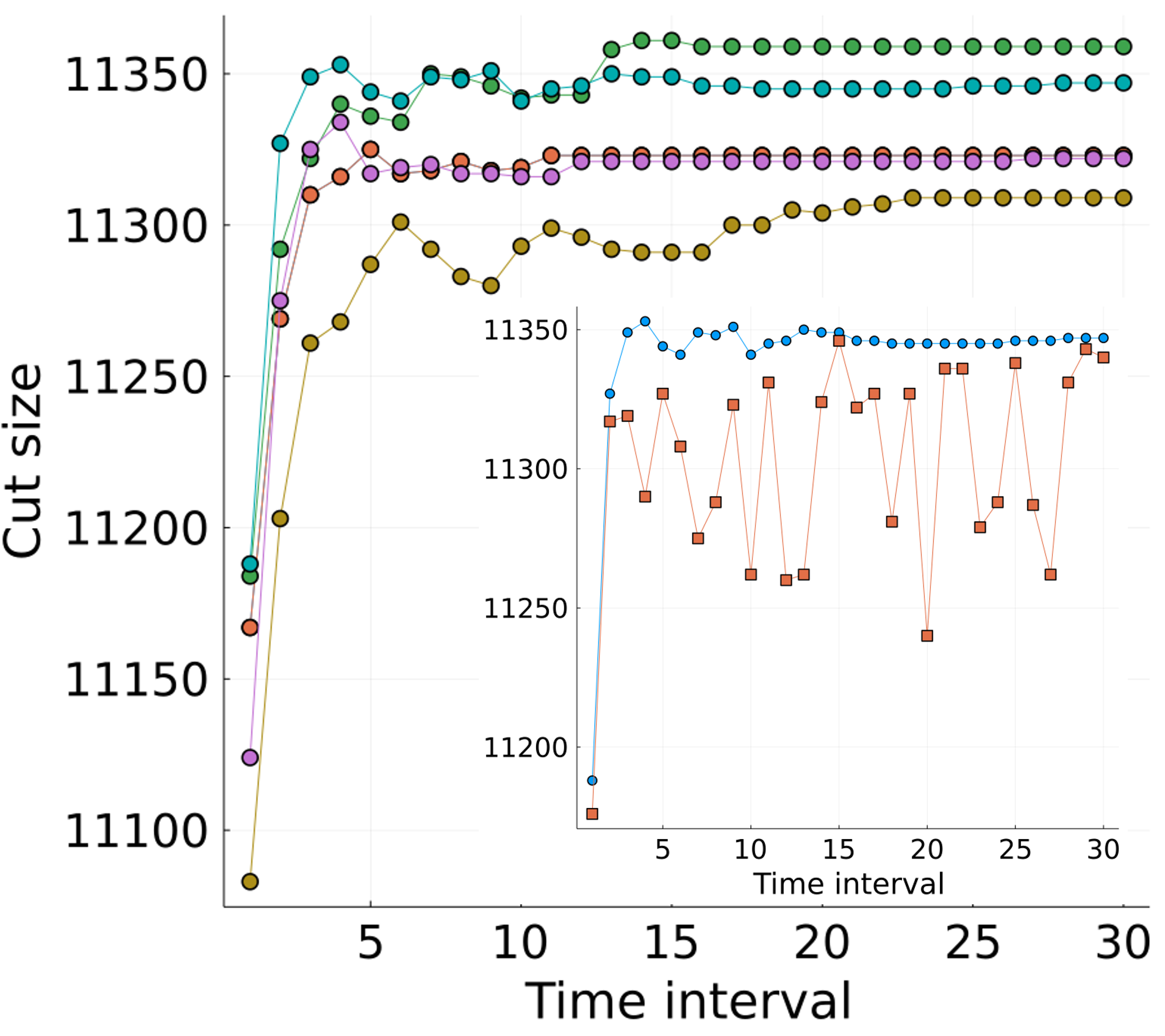
Figure 5: The time evolution of the cut of graph $\mathrm{G}1$. The main panel shows the results of the evolution starting from five random initial configurations. The inset compares the optimal rounding (marked by circles) with the random rounding (marked by squares).

In the simulation outlined in Fig. 3, the Ising machine runs freely for $250$ time steps, each $140K/N$ long. The binary state obtained after optimal rounding are processed further using the local search. First, it is ensured that all nodes satisfy the node majority rule (NMR), that is $F_{m}\geq 0$ for all $m\in\mathcal{V}$. Then, it is ensured that cut edges obey the edge majority rule (EMR), which emerges while applying NMR to the pairs of nodes incident to a cut edge. Let edge $(i,j)$ be cut. Then, the number of cut edges adjacent to $(i,j)$ must exceed the number of uncut edges at least by $2$. Otherwise, reverting $\sigma_{i}$ and $\sigma_{j}$ will increase cut. We denote the finally obtained cut by $C_{F}$. The whole procedure is repeated $100$ times and the best results are kept.

The results of the simulation on $\left\{0,1\right\}$-weighted graphs from Gset gset are presented in Table 1, where they are compared with solutions of the max-cut problem found by optimizer Circut Burer2002Rank-twoPrograms implementing rank-$2$ SDP followed by the local search (the same as described above). While not all Circut numbers are the best among known for GSet (see, for example, benlic_BreakoutLocal_2013 ), the deviations are sufficiently small.

Table 1: The performance of the Ising machine based on triangular model compared to Circut Burer2002Rank-twoPrograms

Test graph ($N$ : $M$)	Triangular model machine			Circut
	Random, $C_{R}$	Optimal, $C_{O}$	Processed, $C_{F}$
G1 (800 : 19176)	10052	10113	11524	11624
G2 (800 : 19176)	9984	9993	11534	11620
G3 (800 : 19176)	10010	10034	11447	11622
G4 (800 : 19176)	10308	10379	11582	11646
G5 (800 : 19176)	10088	10146	11522	11631
G22 (2000 : 19990)	13066	13092	13249	13353
G23 (2000 : 19990)	13068	13084	13202	13332
G24 (2000 : 19990)	13038	13061	13207	13324
G25 (2000 : 19990)	13042	13046	13239	13329
G26 (2000 : 19990)	13044	13054	13225	13321
G43 (1000 : 9990)	6334	6348	6604	6659
G44 (1000 : 9990)	6312	6321	6591	6648
G45 (1000 : 9990)	6343	6347	6594	6653
G46 (1000 : 9990)	6341	6358	6585	6645
G47 (1000 : 9990)	6343	6391	6573	6656
G48 (3000 : 6000)	5722	5728	5746	6000
G49 (3000 : 6000)	5750	5752	5774	6000
G50 (3000 : 6000)	5690	5694	5736	5880
G51 (1000 : 5909)	3640	3659	3786	3846
G52 (1000 : 5916)	3650	3666	3792	3847
G53 (1000 : 5914)	3660	3672	3793	3846
G54 (1000 : 5916)	3773	3667	3788	3850

To estimate how the running time of the machine scales with the size of the problem and how the processing techniques affect the practical machine performance, we apply the machine to a series of random Erdős-Rényi graphs $\mathcal{G}_{N,p}$, where $N$ is the number of graph nodes, and $p$ is the edge presence probability. The ensemble was obtained by sampling five graph for each $N$ in $\left(200,400,600,\ldots,4000\right)$ and $p$ in $\left(0.05,0.1,\ldots,0.35\right)\cup\left(0.12,0.17,\ldots,0.32\right)$. In each simulation, the machine ran freely from a weak perturbation of the best configuration found so far (for the first run of each graph, the best configuration was taken with all spins up). The machine ran $50$ time-steps, each $50\ K/N$ long. The resultant state was optimally rounded and then further post-processed. The found cut is compared to the best found. For each graph, the procedure was repeated $30$ times. The results of the simulation are shown in Fig. 6 depicting the running time and the deviation of the obtained cut values from the Circut’s results versus the number of edges in the graphs.

The dynamical part of looking for the maximal cut requires the fixed number of steps with the number of arithmetic operations determined by the number of edges and, therefore, scales as $\mathcal{O}(M)$. The optimal rounding procedure evaluates the variation of cut while reverting $N-1$ spins and thus also scales as $\mathcal{O}(M)$.

The main contribution of the post-processing procedures to the running time scaling is due to enforcing the EMR, which evaluates the vicinities of cut edges, whose number scales as $M$, and, consequently, has the-worst-case-scenario scaling $\mathcal{O}(M^{5/2})$. To estimate the effect of enforcing the EMR for Erdős-Rényi graphs, we compare in Fig. 6 implementations including both post-processing procedures and enforcing EMR only. The numerical data shows the transition to the faster running time growth (from $\mathcal{O}(M)$ to $\mathcal{O}(M^{2})$). It must be emphasized that for graphs of moderate size ($M>10^{6}$) abandoning the last step in post-processing speeds up the machine by more than the order of magnitude while leading to a fraction of percent loss of accuracy.

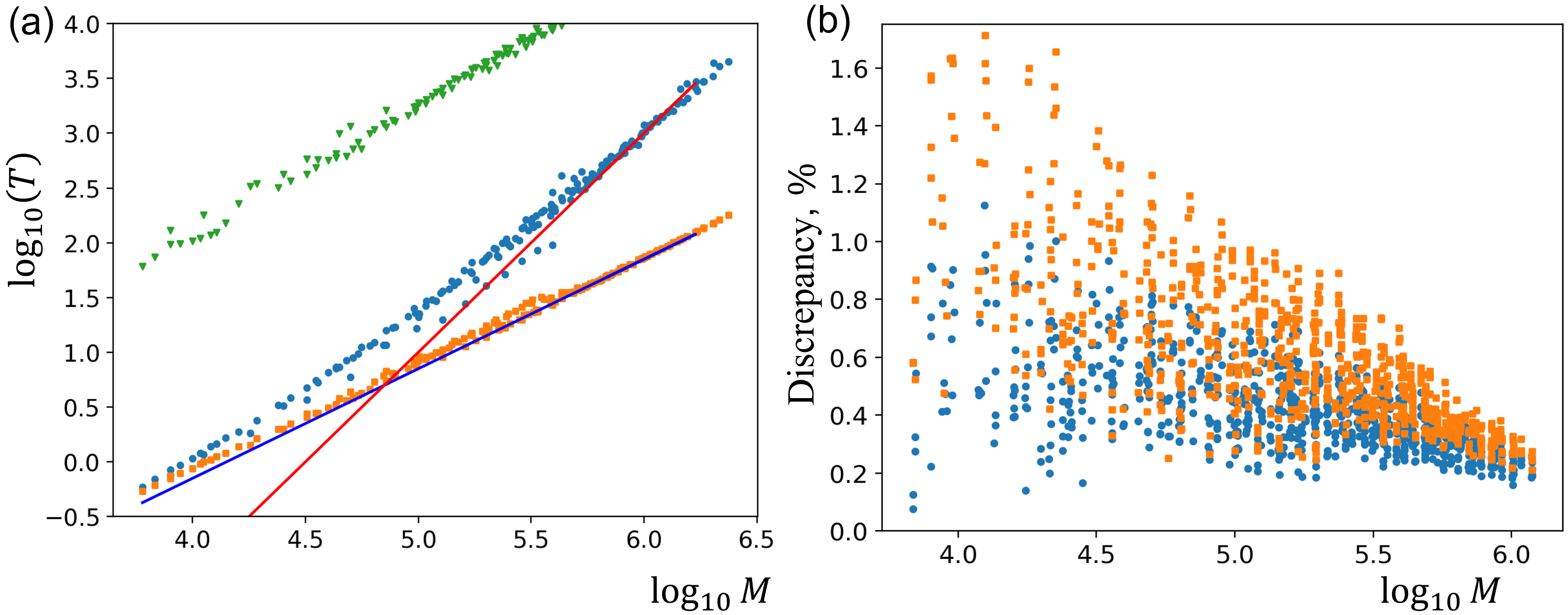
Figure 6: (a) The variation of the running time (the wall-time measured in seconds) with increasing of the size for an ensemble of random Erdős-Rényi graphs $\mathcal{G}_{N,p}$: (circles) full, NMR and EMR, post-processing, (squares) reduced, NMR only, post-processing, (triangles) Circut’s results. The straight lines show scaling $T\propto M^{2}$ and $T\propto M$. (b) The discrepancy between the results using the almost-linear Ising machine with (circles) full and (squares) reduced post-processing.

4 CMOS implementation of the almost-linear Ising machine

The almost-linear character of the dynamics of the Ising machine significantly simplifies a circuit implementation, which can be based on the Euler approximation of the almost-linear Ising machine described by Eq. (9):

$$\Delta v_{i}\left[n+1\right]=-K\sum_{j=1}^{N}w_{ij}\phi\left(v_{i}[n]-v_{j}[n]\right)+K_{s}\phi\left(2v_{i}[n]\right).$$ (22)

Here, $v_{i}$ and $v_{j}$ are dynamical variables, $w_{ij}$ is the weight parameter, $n$ is the time-step number, and $\phi(v)$ is the triangular coupling function defined in Eq. (14).

4.1 Architectural overview

The essential components of the circuit implementation of the almost-linear Ising machine are the vertex elements, a shared (periodic) coupler and the adjacency memory. Their interconnection is shown in Fig. 7(a).

Inside each vertex, a capacitor is employed as the analog spin memory functioning as an analog accumulator. We use a differential current-mode read of the vertices because the majority of operations in Eq. (22) can be broken down into several summations and sign-inversions of analog signals. The first key operation in Eq. (22) is the pairwise subtraction of states. Currents from a pair of vertices are easily subtract if the sinking node is held at a nearly fixed voltage. The second key operation is the piece-wise linear triangular coupling function ($\phi$). A current-mode read enables a straightforward realization of $\phi$, as it may be described as a sum of uniformly spaced currents followed by sign-inversions.

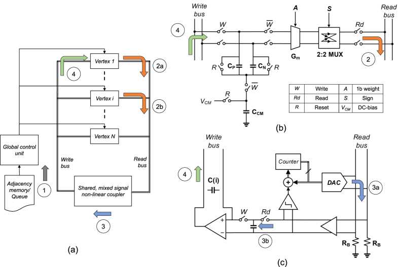
Figure 7: The proof-of-concept implementation of the almost linear Ising machine. (a) Top-level block-diagram of the solver and enumerated signal-flows. (b) Vertex schematic, with the signals of (a) identified. Circuit elements are labeled in bold and binary control-signals in italics. The table lists the signals’ names. Any control signal’s ON state closes the corresponding switch. (c) Non-linear coupler’s block-diagram, with the signal-flows of (a) identified. Step 3 is split into two sub-steps, 3a and 3b. 3a is the application of current components and 3b is the buffering of bus-voltage into the input capacitor.

A current-bus runs next to all vertices, (i) to carry the current originating from the vertices towards the coupler, and (ii) to carry the state increments ($\Delta v_{ij}$) from the coupler to the vertices. As shown in Fig. 7(a), the bus is split into a write-bus and read-bus for simplifying the decoding logic in the spin cell. To realize the triangular coupling ($\phi$), the coupler senses the net current on the bus and alters it by generating and superposing its own current. Additional circuit components, discussed later, translate the net bus-current to state increments. The adjacency memory stores weights from the weighted adjacency matrix ($w_{ij}$) of the graph.

The key operations, depicted in Fig. 7(a–c), are:

1. [(i)]

2. reading the adjacency memory to get $\{i,j\}$ pair for each $w_{ij}=1$,

3. enabling the reading of vertices $i$ and $j$, by enabling the corresponding trans-conductance (Gm) cells,

4. application of the coupling current and reading the steady-state current on the bus,

5. updating the state capacitor’s charge of vertex $i$.

The circuit-level details of each of the components are discussed next.

4.2 Design methodology and details

4.2.1 Vertex

The schematic along with the operational signals of the vertex — read, write, reset, labelled as R, W, and Rd are shown in Fig. 7(b), next to the corresponding switches. The vertex comprises:

1. [(i)]

2. State capacitors: Three capacitors, arranged in a T, are used to store the analog states. $C_{P}$ and $C_{N}$ store charge/voltage in a differential form. $C_{CM}$ stores the common-mode voltage that provides a steady bias for the Gm-cell. Reset switches reset $C_{P}$ and $C_{N}$ to have zero charge and $C_{CM}$ to $V_{CM}$. A switch blocks the charge/discharge of $C_{CM}$ during the update-phase and is enabled only during the read-phase.

3. 1-bit differential Gm-cell: The cell reads the state voltage and supplies a proportional current onto the bus. To conserve area, we use a basic differential-pair with a tail source (Fig. 8). The input transistor pair is biased by the common-mode capacitor. The tail-source is biased externally, with a global biasing voltage. Two identical differential pairs are used, where the second pair, when enabled, allows pre-multiplication with a factor two of the anisotropy term of Eq. (22).

4. Sign-inverter: The opposite signs of $v_{i}$ and $v_{j}$ in Eq. (22) necessitates means to invert the sign/direction of vertex current. For inverting the currents, a 2-way in and 2-way out MUX was used which swaps the current into the bus.

5. Vertex read-enable switch: This switch enables/disables the vertex current onto the bus.

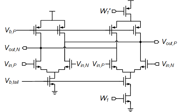
Figure 8: $1$-bit Gm-cell’s transistor-level schematic. $V_{in,P}$ and $V_{in,N}$ are the differential inputs, $V_{out,P}$ and $V_{out,N}$ the differential outputs, $W_{1}$ the digital input, $V_{b,P}$ and $V_{b,tail}$ the global bias-voltages. The left branch is active regardless of digital input. The second branch is active for $W_{1}=1$.

Assuming DRAM capacitor size of 10$\lambda^{2}$ requires refresh time of 1 $\mu$s, where $\lambda$ is the minimum feature size, we use capacitors with size at least $10^{3}\times$ bigger than DRAM size, so that it works without refreshing as it operates for the worst-case time-scale of $1$ ms. For a commercial $130$ nm technology, this is equivalent to a capacitor of about $10$ fF and an area of at least $10^{4}\lambda^{2}$.

4.2.2 Spin-coupler

It consists of three components: digital counter, comparator, and sign-inverter. The counter, depending on the comparator output, changes its state to execute the following operation:

$$\min_{m}\left|I_{i}-I_{j}-mI_{0}\right|,$$ (23)

where, $m$ is an integer denoting the counter’s state, $I_{i}$ and $I_{j}$ denote the currents from the vertices and $I_{0}$ denotes the smallest positive zero of the coupling function. Instead of linear search, faster search methods may be used. As shown in the Fig. 7(c), counter value is converted to an analog current and added to the net branch-current. An additional current inverter is enabled when $m$ is an even number to invert the slope of the linear segments in the coupling function.

The number of segments in the coupling function determines the number of bits required by the counter and by the DAC. It can be shown that if the function is to be composed of $n$ periods, then $\lceil{\log_{2}{4n}}\rceil$ bits are required. If charge increment at each time-step is sufficiently small, limited number of periods (or, peaks) in the non-linear coupling function are required. For our demonstration, we used 3 periods, or a 4-bit DAC.

4.2.3 Switched capacitor based accumulator

To implement the accumulation of Eq. (22), we use a simplified switched capacitor setup Razavi2002DesignCircuits — an operational amplifier with single-ended output, a buffer/input capacitor and the state-capacitor as the accumulator (Fig. 7(c)). At each sampling-instant, an input capacitor stores the amplified output of the current-bus (step 3b in Fig. 7(c)). This is followed by a writing-instant, wherein the same charge is pushed up into the state-capacitor (step 4 in Fig. 7(c)).

To implement different charge increments for the coupling and anisotropy term ($K$ and $K_{s}$ terms in Eq. (22), respectively), two different capacitors must serve at the input of the op-amp. For this reason, we use a programmable capacitor combination (Fig. 8). Since $K_{s}$ is typically smaller than $K$, for anisotropy increments, a smaller input capacitor in series with the branch is activated so that a relatively small charge is pushed into the vertex. Similarly, the overall scale of the increments may be decreased for larger graphs by activating even smaller capacitors in series with the branch.

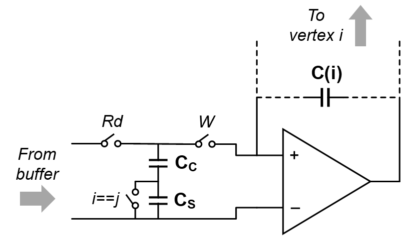
Figure 9: Switched capacitor arrangement for realizing accumulation. ‘Rd’ pulse mirrors the bus voltage as a charge. ‘W’ pulse pushes the entire charge into the state-capacitor. For anisotropic increments ($i=j$), the input capacitance is adjusted appropriately.

4.2.4 State-initializer

In the vertex element presented above, the initial charge on the state capacitor is set to zero which, according to Eq. 22, may prevent the system from ever evolving. For this reason and to facilitate a better exploration of the energy landscape, the state-voltages must be set to random values. We use a 4-bit pseudo-random bit sequence generator (PRBSG) to generate a random bit sequence. A shared DAC converts PRBSG output to the state-capacitor’s voltage. Since the output sequence of PRBSG consists of equi-probable 1 and 0, the initial charge on the state-capacitor is uniformly distributed. It suffices for the initial capacitor voltage to be within the first linear segment of the signed-modulo coupling function. Therefore, all of the bits input to DAC are of lower significance than the bits used in the periodic coupler.

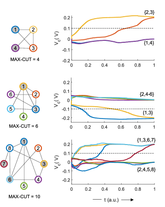
Figure 10: Max-cut results obtained for the three graphs shown on the left. The time variation of state variables corresponding to each vertex is shown on the right by curves of matching colors. The shaded and hollow vertices belong to different sets in the max-cut partition. The dashed lines show the threshold capacitor voltage separating vertices between the partitions.

4.3 Software-equivalence test

We used the IM for solving max-cut problem on randomly connected graphs. Due to long simulation times, we simulated up to 8 nodes, each with a random initial state. Figure 10 plots the evolution of analog spins ($V_{C}$) corresponding to each vertex. On reaching the zeros of the coupling function (200 mV), state-voltages did not change significantly. The partition corresponding to the maximal-cut was found using thresholds of $\pm 100$ mV. With $K_{s}/K$ in Eq. (22) set to 1, one run was enough for finding the maximal cut for the selected graphs. Correct determination of the max-cut values for the graphs verifies the software-equivalence for the proposed hardware.

The proposed design can be further refined to facilitate large node integration. For instance, the current bus can be segmented to improve coupling between on-chip distant nodes. Another refinement could involve the use of alternative methodologies to activate vertices. The current design uses de-multiplexers to enable/disable vertex reads, and, as a result, only one vertex can be read at a time. A serial communication scheme may be employed to enable reading multiple vertices at a time and activating only relevant bus segments. The segmentation would also pave the way for parallel and independent coupling calculations, and speeding up the dynamics. These additions would not significantly affect the area-per-spin, which is dominated by the area of the state-capacitors.

5 Conclusion

The Ising model of computation reformulates computing tasks as set partitioning problems and, subsequently, as the Ising model ground state problem. It presents a promising way to find and implement efficient heuristics to NP-hard combinatorial optimization problems. To compete with solving these problems on general-purpose computers, however, the prospective architectures based on the Ising model of computation must support a large number, billions and more, of spins. Achieving such a high degree of integration encounters not only technological but also fundamental challenges. For example, the underlying dynamical model must be, on the one hand, sufficiently simple to reduce sensitivity to unavoidable variations of components characteristics. On the other hand, the model should not sacrifice computational capabilities. To tackle the problems posed by large architectures, the present paper explores engineering the dynamical model governing the Ising machine.

We show that Ising machines based on Kuramoto networks of nonlinear oscillators implement the dynamics of the XY model, which, in turn, corresponds to the gradient-descent solution of the rank- $\ignorespaces 2$ semidefinite programming (SDP) relaxation of the Ising model. This chain of equivalences puts developing Ising machines into the context of the combinatorial optimization theory and highlights the dynamical elements enabling the computational resource.

Building on these findings, we consider an approximation of the XY model by unconstrained dynamical variables with piece-wise linear coupling (almost-linear Ising machine). We show that the introduced dynamical model, which we call the triangular model, is characterized by the integrality gap close to the canonical Goemans-Williamson ratio. Thus, the binary configuration recovered from the ground state of the triangular model is close to the ground state of the Ising model. Comparison on a set of benchmark problems showed that the Ising solver based on the triangular model provides solutions with the quality on par with Circut, one of the best max-cut heuristic solvers dunningWhat2018 , even when the machine runs unsupervised (without any preprocessing and intermediate controls).

We study the scaling properties of the almost-linear Ising machine on an ensemble of random Erdős-Rényi graphs $\mathcal{G}_{N,p}$ with $200\leq N\leq 4000$ and $0.05\leq p\leq 0.35$ and compare its performance with Circut. We show that the running time of the machine scales polynomially with the size of the problem. On moderately sized problems (with the number of edges exceeding $10^{5}$), the almost-linear Ising machine showed orders of magnitude speed up compared to Circut with below one percent solution discrepancy.

To demonstrate opportunities provided by the almost-linear dynamical models for hardware realizations, we investigate a proof-of-concept circuit implementation and verify it using the device-level simulation. Thanks to the simplicity of the dynamics, the designed architecture demonstrates small area per spin, increased state programmability, and flexibility to simulate all-to-all connected graphs.

Acknowledgments

The work has been supported by the US National Science Foundation (NSF) under Grant No. 1710940 and by the US Air Force Office of Scientific Research (AFOSR) under Grant No. FA9550-16-1-0363.

References

- \bibcommenthead
- (1) Babbush, R., Perdomo-Ortiz, A., O’Gorman, B., Macready, W., Aspuru-Guzik, A.: Construction of Energy Functions for Lattice Heteropolymer Models: Efficient Encodings for Constraint Satisfaction Programming and Quantum Annealing, pp. 201–244 (2014). https://doi.org/%****␣main.tex␣Line␣1125␣****10.1002/9781118755815.ch05. https://onlinelibrary.wiley.com/doi/10.1002/9781118755815.ch05
- (2) Fraenkel, A.S.: Complexity of protein folding. Bulletin of Mathematical Biology 55(6), 1199–1210 (1993). https://doi.org/10.1007/BF02460704
- (3) Wang, J., MacKenzie, J.D., Ramachandran, R., Zhang, Y., Wang, H., Chen, D.Z.: Segmenting Subcellular Structures in Histology Tissue Images, pp. 556–559 (2015). https://doi.org/10.1109/ISBI.2015.7163934
- (4) Barahona, F.: On the computational complexity of Ising spin glass models. J. Phys.A: Math. Gen. 15(10), 3241–3253 (1982). https://doi.org/10.1088/0305-4470/15/10/028
- (5) Karp, R.M.: Reducibility among Combinatorial Problems. In: Miller, R.E., Thatcher, J.W., Bohlinger, J.D. (eds.) Complexity of Computer Computations, pp. 85–103. Springer, Boston, MA (1972). https://doi.org/10.1007/978-1-4684-2001-2_9
- (6) Garey, M.R., Johnson, D.S., Stockmeyer, L.: Some simplified NP-complete graph problems. Theoretical Computer Science 1(3), 237–267 (1976). https://doi.org/%****␣main.tex␣Line␣1200␣****10.1016/0304-3975(76)90059-1
- (7) Lucas, A.: Ising formulations of many NP problems. Frontiers in Physics 2(February), 1–14 (2014). https://doi.org/10.3389/fphy.2014.00005
- (8) Kirkpatrick, S., Gelatt, C.D., Vecchi, M.P.: Optimization by Simulated Annealing. Science 220(4598), 671–680 (1983). https://doi.org/10.1126/science.220.4598.671
- (9) Yamaoka, M., Yoshimura, C., Hayashi, M., Okuyama, T., Aoki, H., Mizuno, H.: 20k-spin Ising chip for combinational optimization problem with CMOS annealing. Digest of Technical Papers - IEEE International Solid-State Circuits Conference 58, 432–433 (2015). https://doi.org/10.1109/ISSCC.2015.7063111
- (10) Takemoto, T., Hayashi, M., Yoshimura, C., Yamaoka, M.: A 2 x 30k-Spin Multi-Chip Scalable CMOS Annealing Processor Based on a Processing-in-Memory Approach for Solving Large-Scale Combinatorial Optimization Problems. IEEE Journal of Solid-State Circuits 55(1), 145–156 (2020). https://doi.org/10.1109/JSSC.2019.2949230
- (11) Su, Y., Kim, H., Kim, B.: 31.2 CIM-Spin: A 0.5-to-1.2V scalable annealing processor using digital compute-in-memory spin operators and register-based spins for combinatorial optimization problems. In: 2020 IEEE International Solid-State Circuits Conference - (ISSCC), pp. 480–482 (2020). https://doi.org/10.1109/ISSCC19947.2020.9062938
- (12) Takemoto, T., Yamamoto, K., Yoshimura, C., Hayashi, M., Tada, M., Saito, H., Mashimo, M., Yamaoka, M.: 4.6 A 144kb annealing system composed of 9×16Kb annealing processor chips with scalable chip-to-chip connections for large-scale combinatorial optimization problems. In: 2021 IEEE International Solid- State Circuits Conference (ISSCC), vol. 64, pp. 64–66 (2021). https://doi.org/10.1109/ISSCC42613.2021.9365748
- (13) Okuyama, T., Yoshimura, C., Hayashi, M., Yamaoka, M.: Computing architecture to perform approximated simulated annealing for Ising models. In: 2016 IEEE International Conference on Rebooting Computing (ICRC), pp. 1–8 (2016). https://doi.org/10.1109/ICRC.2016.7738673
- (14) Yamamoto, K., Huang, W., Takamaeda-Yamazaki, S., Ikebe, M., Asai, T., Motomura, M.: A Time-Division Multiplexing Ising Machine on FPGAs. ACM International Conference Proceeding Series (2017). https://doi.org/10.1145/3120895.3120905
- (15) Ahmed, I., Chiu, P.W., Moy, W., Kim, C.H.: A Probabilistic Compute Fabric Based on Coupled Ring Oscillators for Solving Combinatorial Optimization Problems. IEEE Journal of Solid-State Circuits, 1–11 (2021). https://doi.org/10.1109/JSSC.2021.3062821
- (16) Bashar, M.K., Mallick, A., Truesdell, D.S., Calhoun, B.H., Joshi, S., Shukla, N.: Experimental Demonstration of a Reconfigurable Coupled Oscillator Platform to Solve the Max-Cut Problem. IEEE Journal on Exploratory Solid-State Computational Devices and Circuits 6(2), 116–121 (2020). https://doi.org/%****␣main.tex␣Line␣1375␣****10.1109/JXCDC.2020.3025994
- (17) Parihar, A., Shukla, N., Jerry, M., Datta, S., Raychowdhury, A.: Vertex coloring of graphs via phase dynamics of coupled oscillatory networks. Scientific Reports 7(1), 911 (2017). https://doi.org/10.1038/s41598-017-00825-1
- (18) Raychowdhury, A., Parihar, A., Smith, G.H., Narayanan, V., Csaba, G., Jerry, M., Porod, W., Datta, S.: Computing With Networks of Oscillatory Dynamical Systems. Proceedings of the IEEE 107(1), 73–89 (2019). https://doi.org/10.1109/JPROC.2018.2878854
- (19) Marandi, A., Wang, Z., Takata, K., Byer, R.L., Yamamoto, Y.: Network of time-multiplexed optical parametric oscillators as a coherent Ising machine. Nature Photonics 8(12), 937–942 (2014). https://doi.org/10.1038/nphoton.2014.249
- (20) McMahon, P.L., Marandi, A., Haribara, Y., Hamerly, R., Langrock, C., Tamate, S., Inagaki, T., Takesue, H., Utsunomiya, S., Aihara, K., Byer, R.L., Fejer, M.M., Mabuchi, H., Yamamoto, Y.: A fully programmable 100-spin coherent Ising machine with all-to-all connections. Science 354(6312), 614–617 (2016). https://doi.org/10.1126/science.aah5178
- (21) Böhm, F., Verschaffelt, G., Van der Sande, G.: A poor man’s coherent Ising machine based on opto-electronic feedback systems for solving optimization problems. Nature Communications 10(1), 3538 (2019). https://doi.org/10.1038/s41467-019-11484-3
- (22) Leleu, T., Yamamoto, Y., Utsunomiya, S., Aihara, K.: Combinatorial optimization using dynamical phase transitions in driven-dissipative systems. Physical Review E 95(2), 4–6 (2017). https://doi.org/10.1103/PhysRevE.95.022118
- (23) Molnár, B., Molnár, F., Varga, M., Toroczkai, Z., Ercsey-Ravasz, M.: A continuous-time MaxSAT solver with high analog performance. Nature Communications 9(1), 1–12 (2018). https://doi.org/10.1038/s41467-018-07327-2
- (24) Afoakwa, R., Zhang, Y., Vengalam, U.K.R., Ignjatovic, Z., Huang, M.: BRIM: Bistable resistively-coupled ising machine. In: 2021 IEEE International Symposium on High-Performance Computer Architecture (HPCA), pp. 749–760. IEEE, Seoul, Korea (South) (2021). https://doi.org/10.1109/HPCA51647.2021.00068
- (25) Gset: Group of Random Graphs. https://sparse.tamu.edu/Gset
- (26) Papadimitriou, C.H., Yannakakis, M.: Optimization, approximation, and complexity classes. Journal of Computer and System Sciences 43(3), 425–440 (1991). https://doi.org/10.1016/0022-0000(91)90023-X
- (27) Khot, S., Kindler, G., Mossel, E., O’Donnell, R.: Optimal Inapproximability Results for Max-Cut and Other 2-Variable CSPs? In: 45th Annual IEEE Symposium on Foundations of Computer Science, pp. 146–154. IEEE, Rome, Italy (2004). https://doi.org/10.1109/FOCS.2004.49
- (28) Hamerly, R., Inagaki, T., McMahon, P.L., Venturelli, D., Marandi, A., Onodera, T., Ng, E., Langrock, C., Inaba, K., Honjo, T., Enbutsu, K., Umeki, T., Kasahara, R., Utsunomiya, S., Kako, S., Kawarabayashi, K.-i., Byer, R.L., Fejer, M.M., Mabuchi, H., Englund, D., Rieffel, E., Takesue, H., Yamamoto, Y.: Experimental investigation of performance differences between coherent Ising machines and a quantum annealer. Science Advances 5(5), 0823 (2019). https://doi.org/10.1126/sciadv.aau0823
- (29) Leleu, T., Khoyratee, F., Levi, T., Hamerly, R., Kohno, T., Aihara, K.: Scaling advantage of chaotic amplitude control for high-performance combinatorial optimization. Communications Physics 4(1), 266 (2021). https://doi.org/10.1038/s42005-021-00768-0
- (30) Erementchouk, M., Shukla, A., Mazumder, P.: On computational capabilities of Ising machines based on nonlinear oscillators. Physica D: Nonlinear Phenomena 437, 133334 (2022). https://doi.org/10.1016/j.physd.2022.133334
- (31) Adler, R.: A Study of Locking Phenomena in Oscillators. Proceedings of the IRE 34(6), 351–357 (1946). https://doi.org/10.1109/JRPROC.1946.229930
- (32) Bhansali, P., Roychowdhury, J.: Gen-Adler: The generalized Adler’s equation for injection locking analysis in oscillators. In: 2009 Asia and South Pacific Design Automation Conference, pp. 522–527. IEEE, Yokohama, Japan (2009). https://doi.org/10.1109/ASPDAC.2009.4796533
- (33) Korte, B., Vygen, J.: Combinatorial Optimization. Algorithms and Combinatorics, vol. 21. Springer Berlin Heidelberg, Berlin, Heidelberg (2018). https://doi.org/10.1007/978-3-662-56039-6
- (34) Goemans, M.X., Williamson, D.P.: Improved approximation algorithms for maximum cut and satisfiability problems using semidefinite programming. Journal of the ACM 42(6), 1115–1145 (1995). https://doi.org/10.1145/227683.227684
- (35) Alon, N., Sudakov, B.: Bipartite Subgraphs and the Smallest Eigenvalue. Combinatorics, Probability and Computing 9(1), 1–12 (2000). https://doi.org/10.1017/S0963548399004071
- (36) Deza, M.M., Laurent, M.: Geometry of Cuts and Metrics. Algorithms and Combinatorics, vol. 15. Springer Berlin Heidelberg, Berlin, Heidelberg (1997). https://doi.org/10.1007/978-3-642-04295-9
- (37) Burer, S., Monteiro, R.D.C., Zhang, Y.: Rank-two relaxation heuristics for MAX-CUT and other binary quadratic programs. SIAM Journal on Optimization 12(2), 503–521 (2002). https://doi.org/10.1137/S1052623400382467
- (38) Laurent, M., Poljak, S.: On a positive semidefinite relaxation of the cut polytope. Linear Algebra and its Applications 223-224, 439–461 (1995). https://doi.org/10.1016/0024-3795(95)00271-R
- (39) Charikar, M., Wirth, A.: Maximizing quadratic programs: Extending grothendieck’s inequality. In: 45th Annual IEEE Symposium on Foundations of Computer Science, pp. 54–60. IEEE, Rome, Italy (2004). https://doi.org/10.1109/FOCS.2004.39
- (40) Alon, N., Naor, A.: Approximating the cut-norm via Grothendieck’s inequality. In: Proceedings of the Thirty-Sixth Annual ACM Symposium on Theory of Computing - STOC ’04, p. 72. ACM Press, Chicago, IL, USA (2004). https://doi.org/10.1145/1007352.1007371
- (41) Anjos, M.F., Wolkowicz, H.: Strengthened semidefinite relaxations via a second lifting for the Max-Cut problem. Discrete Applied Mathematics 119(1-2), 79–106 (2002). https://doi.org/10.1016/S0166-218X(01)00266-9
- (42) Benlic, U., Hao, J.-K.: Breakout Local Search for the Max-Cutproblem. Engineering Applications of Artificial Intelligence 26(3), 1162–1173 (2013). https://doi.org/10.1016/j.engappai.2012.09.001
- (43) Razavi, B.: Design of Analog CMOS Integrated Circuits, p. 684. Tata McGraw-Hill, USA (2002)
- (44) Dunning, I., Gupta, S., Silberholz, J.: What Works Best When? A Systematic Evaluation of Heuristics for Max-Cut and QUBO. INFORMS Journal on Computing 30(3), 608–624 (2018). https://doi.org/10.1287/ijoc.2017.0798