Superdiffusion in random two dimensional system with time-reversal symmetry and long-range hopping

Abstract

Although it is recognized that Anderson localization takes place for all states at a dimension $d$ less or equal $2$, while delocalization is expected for hopping $V(r)$ decreasing with the distance slower or as $r^{-d}$, the localization problem in the crossover regime for the dimension $d=2$ and hopping $V(r)\propto r^{-2}$ is not resolved yet. Following earlier suggestions we show that for the hopping determined by two-dimensional anisotropic dipole-dipole interactions in the presence of time-reversal symmetry there exist two distinguishable phases at weak and strong disorder. The first phase is characterized by ergodic dynamics and superdiffusive transport, while the second phase is characterized by diffusive transport and delocalized eigenstates with fractal dimension less than $2$. The transition between phases is resolved analytically using the extension of scaling theory of localization and verified numerically using an exact numerical diagonalization.

I Introduction.

Low dimensional systems with a dimension $d\leq 2$ possessing the time-reversal symmetry are critical in the Anderson localization problem [1]. All states there must be exponentially localized at arbitrarily small disorder strength as was shown using the scaling theory of localization [2], analysis of conductivity [3] and extensive numerical simulations [4; 5] (see also reviews [6; 7; 8]). This localization is originated from the singular backscattering due to random potential dramatically enhanced in low dimension $d\leq 2$ where random paths inevitably return to the origin [7].

The scaling theory of localization suggests the single parameter scaling for the dimensionless conductance $C=G/(e^{2}/\hbar)$ dependence on the size $L$ in the form [2; 3] ($G$ is the conductance)

$$\frac{d\ln(C)}{d\ln(L)}=\beta(C),$$

$$\beta(C)=-\frac{c_{loc}}{C}+O(C^{-4}),~{}c_{loc}=\frac{1}{2\pi^{2}},$$ (1)

where the $\beta$-function has been evaluated using expansion of the equivalent non-linear sigma-model [9; 8] valid at $C\gg c_{loc}$. Eq. (1) predicts the reduction of conductance with the system size $L$ as $C(L)=C_{0}-c_{loc}\ln(L)$ where $C_{0}$ is the conductance at the lower cutoff $L=1$. Logarithmic reduction of conductance with the system size results in the inevitable localization at large sizes $L$.

This universal scaling is limited to systems with a short-range hopping, while the hopping decreasing with the distance as $V(\mathbf{r})\propto r^{-d}$ or slower leads to delocalization of all states [1; 10; 11; 12; 13; 14] except for the marginal case of diverging Fourier transform of a hopping amplitude [15; 16; 17; 18; 19; 20; 21; 22; 23; 24; 25; 26]. If disorder is strong, eigenstates of the problem with the long-range hopping $V(\mathbf{r})\propto r^{-d}$ possess a multifractal structure and the time dependent displacement of the particle $r$ obeys the law $r\propto t^{1/d}$, which is subdiffusive in $3D$ [11], diffusive in $2D$ and superdiffusive in $1D$ [12]. The long-range hopping $V(\mathbf{r})\propto r^{-2}$ is ubiquitous in pure two-dimensional systems [27], where it can be originated from the virtual exchange by two dimensional photons leading to the $2D$ dipole-dipole interaction [28] or indirect exchange by $2D$ electron-hole pairs leading to $2D$ RKKY interaction [29]. Power-law distant dependent hopping is crucial for the many-body localization problem [30; 31; 32; 33; 34; 35; 36; 37; 38; 39; 40; 41; 42; 43; 44; 45; 46; 47; 48; 49; 50; 51; 52; 53], where long-range interaction can result in localization breakdown at arbitrary disorder.

For the hopping under consideration $r^{-d}$ and weak disorder there is the transition in $3D$ to the standard delocalized phase characterized by the diffusive transport and ergodic dynamics [54], while in $1D$ eigenstates turns out to be multifractals with the dimension smaller than $1$ [12]. $2D$ systems are more complicated, because for the hopping $V(\mathbf{r})\propto r^{-d}$ the dimensionless Drude conductance diverges logarithmically with the system size as $C_{0}(L)=c_{*}\ln(L)$ [28]. Considering the balance of this logarithmic raise of conductance and its logarithmic suppression by coherent back scattering $c_{loc}\ln(L)$ Eq. (1), it was suggested in Ref. [28] that two delocalized phases can exist including the superdiffusive (fast) phase at $c_{*}>c_{loc}$ and the slow phase with diffusive transport at $c_{*}<c_{loc}$ and the phase boundary realized at $c_{*}=c_{loc}$. Yet it turns out that in systems, possessing time-reversal symmetry, for isotropic dipoles considered in Ref. [28] $c_{*}<c_{loc}$ for an arbitrarily disorder strength so the fast phase does not exist. This is in contrast with the systems with a broken time-reversal symmetry, possessing the transition between fast and slow phases, characterized by the unstable fixed point [28].

These achievements motivated us to search for the superdiffusive, fast phase using different hopping interaction including anisotropic dipole-dipole interaction with identically oriented dipoles. Our preliminary estimates also show emergence of a superdiffusive phase for the $2D$ RKKY interaction at sufficiently weak disorder that needs a separate consideration. These interactions differ from the isotropic dipole model of Ref. [28] by the presence of dispersive modes with the mean free path increasing unlimitedly with decreasing disorder with similar increase of the logarithmic growth parameter $c_{*}$. This makes the appearance of the fast phase with $c_{*}>c_{loc}$ unavoidable. similarly the anisotropy-mediated localization investigated in Ref. [20] where the number of such modes is extensive, though measure zero.

The transition between phases occurring at $c_{*}=c_{loc}$ differs qualitatively from the typical localization transition since in the present case the renormalization group equation for the conductance possesses the stable fixed point. Consequently, conductance approaches infinity with decreasing disorder strength in a continuous manner and the transition point can be expressed analytically through the single-particle green function. Consequently, we can find the transition point analytically for the model with the Lorentzian distribution of disorder where Green functions can be evaluated exactly, which is unprecendental for the localization problem.

This is in a sharp contrast with the standard localization transition in 3D systems with the short-range hopping [55; 6] and the transition in the system similar to the present one but with a violated time-reversal symmetry [28]. For those models conductance instantaneously jumps from a critical value to infinity at the transition point, that can can be approached only numerically.

Recent experimental realizations of $2D$ Anderson localization [56] and long-range hopping [57] represent the steps towards generating the settings targeted in the present work. Consequently, we believe that its experimental realization is possible and it is strongly encouraged.

We investigate two phases for two-dimensional Anderson model, described in Sec. II with a long-range hopping, formulated below, using the extension of scaling theory of localization for the long-range hopping developed in Sec. III, IV and exact numerical diagonalization in Sec. V. The Lloyd model with the Lorentzian distribution of random site potentials is used since the Green functions can be evaluated exactly in this model [58], and using them we can find analytically the transition between fast and slow phases.

The phase boundary $c_{*}=c_{loc}$ is identified analytically in Secs. III, IV and verified numerically (see Sec. V and Fig. 1 there). Both phases are characterized by level statistics, that is of Wigner-Dyson for the fast phase and intermediate between Poisson and Wigner-Dyson otherwise (see Fig. 2), eigenstate dimension ($2$ for the fast phase and less than $2$ otherwise, as depicted in Fig. 3) and particle transport (superdiffusive or diffusive, see Fig. 4).

II Model

Anderson model in $2D$ is investigated. The Hamiltonian of the model has the form

$$\widehat{H}=\sum_{i,j}V_{ij}c_{i}^{\dagger}c_{j}+\sum_{i}\phi_{i}c_{i}^{\dagger}c_{i},$$ (2)

where the summation is performed over $N=L^{2}$ lattice sites enumerated by indices $i$ with coordinates $\mathbf{r}_{i}=(x_{i},y_{i})$ occupying the periodic square lattice with a period equal to unity placed onto the surface of torus characterized by the radii $R=L/(2\pi)$. Independent random energies $\phi_{i}$ obey the Lorentzian distribution

$$P(\phi)=\frac{1}{\pi}\frac{W}{W^{2}+\phi^{2}},$$ (3)

having the width $W$ characterizing the disorder strength, while hopping amplitudes are given by the exchange of the dipolar excitations between interacting dipoles, oriented along the $x$-axis, via the interaction [28]

$$V(\mathbf{r}_{ij})=V_{0}\frac{x_{ij}^{2}-y_{ij}^{2}}{r_{ij}^{4}},\quad r_{ij}=(x_{ij},y_{ij}).$$ (4)

These hopping terms are formed similarly to the interaction $(3x^{2}-r^{2})/r^{5}$ in three dimensions [59].

For the Lorentzian distribution of random potentials the Green’s functions, averaged over the random potnetial realizations, can be evaluated exactly [58] in the momentum representation as

$$G(E,\mathbf{q})=\frac{1}{E-V(\mathbf{q})-iW},$$

$$V(\mathbf{q})=\sum_{k}V_{jk}e^{i\mathbf{qr}_{jk}},$$ (5)

where $V(\mathbf{q})$ expresses the Fourier transform of the hopping $V_{ik}$. For small wavevectors $q\ll 1$ it is given by the continuous approach that has the form

$$V(\mathbf{q})\approx 2\pi V_{0}\frac{q_{y}^{2}-q_{x}^{2}}{q^{2}}.$$ (6)

as verified in Appendix A numerically, see also Ref. [20]. The Green functions are needed for the calculation of a zeroth order conductance given below. Below we set $V_{0}=1$ and use the effective disorder strength parameter $W$ to distinguish different phases.

III Zeroth order conductance

One can express the zeroth order dimensionless conductance tensor at given energy $E$ using the Kubo formula as [3; 7; 28]

$$C^{(0)}_{ab}=\int\frac{d\mathbf{q}}{\pi(2\pi)^{d}}\left(\frac{\partial V(\mathbf{q})}{\partial q_{a}}\right)\left(\frac{\partial V(\mathbf{q})}{\partial q_{b}}\right)|{\rm Im}G(E,\mathbf{q})|^{2},$$ (7)

where $G(E,\mathbf{q})$ is the retarded Green function at energy $E$ and wavevector $\mathbf{q}$ defined in Eq. (5).

The conductance in Eq. (7) diverges logarithmically at small wavevectors $q\rightarrow 0$ corresponding to the long distances. This divergence is caused by the divergence of the mean squared displacement $\int d^{2}\mathbf{r}V(r)^{2}r^{2}$ within the Fermi-Golden rule approach. At long distances the Fourier transform continuous representation becomes exact so the use of the hopping amplitude Fourier transform in the form of Eq. (6) is completely justified. Below we evaluate the diverging part needed for the characterization of the phase transition for the dipole - dipole interaction.

For the dipole-dipole hopping Eqs. (4), (6) the integral for the zeroth order conductance Eq. (7) diverges logarithmically at $q=0$. For the finite size $L$ the integral should be cutoff at the minimum value $q=\eta/L$, with the parameter $\eta=O(1)$ depending on the specific boundary conditions. Then the conductance tensor diverging components in Eq. (7) can be evaluated with the logarithmic accuracy as $C_{xx}=c_{x}\ln(L)$, $C_{yy}=c_{y}\ln(L)$, $c_{xy}=c_{yx}=0$, where

$$c_{x}=\frac{\partial C^{(0)}_{xx}}{\partial\ln(L)}=\frac{4}{\pi}\int_{0}^{2\pi}d\phi\frac{\cos(\phi)^{2}\sin(\phi)^{4}W^{2}}{\left[(E-\pi\cos(2\phi))^{2}+W^{2}\right]^{2}}$$

$$=\frac{(\pi^{2}-W^{2}-E^{2}){\rm Im}(\sqrt{E^{2}-(\pi-iW)^{2}})+\pi W{\rm Re}(\sqrt{E^{2}-(\pi-iW)^{2}})}{4\pi^{3}\sqrt{(E+\pi)^{2}+W^{2}}},$$

$$c_{y}=\frac{\partial C^{(0)}_{yy}}{\partial\ln(L)}=\frac{4^{2}}{\pi}\int_{0}^{2\pi}d\phi\frac{\cos(\phi)^{4}\sin(\phi)^{2}W^{2}}{\left[(E-\pi\cos(2\phi))^{2}+W^{2}\right]^{2}}$$

$$=\frac{(\pi^{2}-W^{2}-E^{2}){\rm Im}(\sqrt{E^{2}-(\pi-iW)^{2}})+\pi W{\rm Re}(\sqrt{E^{2}-(\pi-iW)^{2}})}{4\pi^{3}\sqrt{(-E+\pi)^{2}+W^{2}}}.$$ (8)

In the middle of the band $E=0$ the conductance is isotropic, $C_{xx}=C_{yy}=c_{*}\ln(L)$, and the logarithmic growth rate $c_{*}$ is given by

$$c_{*}=\frac{1}{2W\sqrt{\pi^{2}+W^{2}}}.$$ (9)

It is noticeable, that in the weak disorder limit ($W\rightarrow 0$) the rate parameter $c_{*}$ in Eq. (9) approaches infinity, so the transition to the superdiffusive regime should take place at a finite disorder strength $W$ where $c_{*}(W)=c_{loc}=1/(2\pi^{2})$ in contrast with the isotropic dipole-dipole hopping [28].

The generalization to the arbitrary distribution of random potentials can be made by the replacements $E\rightarrow E-{\rm Re}\Sigma(E,0)$ and $W\rightarrow-{\rm Im}\Sigma(E,0)$ in Eqs. (8), (9), where $\Sigma(E,0)$ is the self-energy evaluated at energy $E$ and wavevector $q=0$. One should notice that $\Sigma(0,0)=0$. Finding the self-energy for arbitrary distribution of random potentials remains a challenge; yet this problem is much easier compared to the localization problem itself. The zeroth order conductance serves as an input parameter to the renormalization group equation for the conductance derived below.

IV Renormalization group equation.

Here we derive the $\beta$-function determining the size dependence of conductance in Eq. (1) within the one-loop order. The derivation below is given for the isotropic regime of symmetric conductances $c_{xx}=c_{yy}$ while for the anisotropic regime we give the results in the end of the present section. The isotropic regime is approximately valid for the system under consideration at zero energy (see Eq. (9) in Sec. III).

We examine the renormalization of conductance $C(q,p_{1})$ for the orthogonal (possessing the time-reversal symmetry) sigma model within the one-loop order assuming that the conductance is much greater than one, which is true near the transition point, where it approaches infinity. Here $q$ is the current momentum and $p_{1}$ is the maximum momentum [9] reduced during renormalization procedure. The renormalization of the conductance is associated with the reduction of the maximum momentum to the new value $p_{2}\ll p_{1}$. This renormalization can be expressed as [9; 12] ($q\ll p$)

$$q^{2}(C(q,p_{2})-C(q,p_{1}))\approx-\int^{\prime}\frac{d\mathbf{k}}{\pi(2\pi)^{2}}\frac{C(|\mathbf{k}+\mathbf{q}|,p_{1})(\mathbf{k+q})^{2}-C(k,p_{1})k^{2}}{C(k,p_{1})k^{2}},$$ (10)

where integration $\int^{\prime}$ is taken over the domain of momenta $p_{2}<p<p_{1}$ that is getting excluded during the renormalization procedure. This is the one-loop order correction to the conductance similar to Eq. (25) in Ref. [12], where it was considered for a one dimensional model with the long-range hopping. The terms $C(k,p_{1})k^{2}$, $C(|\mathbf{k}+\mathbf{q}|,p_{1})(\mathbf{k+q})^{2}$ in the denominators are identical to the terms $|q+k|^{\sigma}$ and $|k|^{\sigma}$ in Ref. [12].

The initial conditions to Eq. (10) at large $p_{1}=O(1)$ are set using the zeroth order conductance as

$$C(q,1)=c_{*}\ln(1/q),$$ (11)

where the inverse wavevector $q$ serves as the cutoff radius in the definition of the conductance. The long-range interaction enters into the consideration through this initial condition.

In the limit $q\ll p_{1}$ one can expand the expression in the numerator to the second order in $q$ as (the first order disappears because of the integration over angles)

$$C(q,p_{2})-C(q,p_{1})\approx-\sum_{\alpha,\beta=x,y}\frac{q_{\alpha}q_{\beta}}{2q^{2}}\int^{\prime}\frac{d\mathbf{p}}{\pi(2\pi)^{2}}\frac{\partial^{2}(C(p,p_{1})p^{2})}{\partial p_{\alpha}\partial p_{\beta}}\frac{1}{C(p,p_{1})p^{2}}.$$ (12)

Evaluating derivatives and averaging over angles of vector $\mathbf{p}$ we get

$$C(q,p_{2})-C(q,p_{1})=-\int^{\prime}\frac{d\mathbf{p}}{\pi(2\pi)^{2}}\left[C(p,p_{1})+\frac{\partial C(p,p_{1})}{\partial\ln(p)}+\frac{1}{4}\frac{\partial^{2}C(p,p_{1})}{\partial\ln(p)^{2}}\right]\frac{1}{C(p,p_{1})p^{2}}.$$ (13)

Assuming that the logarithmic derivatives of the conductance are smooth functions (this is justified by the logarithmic size dependence of conductance in the initial condition Eq. (11) and can be verified using the solution of the equation) one can perform logarithmic integration in the right hand side of Eq. (13) and express this equation in the standard differential form similarly to Ref. [9]

$$\frac{\partial C(q,p)}{\partial\ln(p)}=\frac{1}{2\pi^{2}}\left[1+\frac{1}{C(p,p)}\frac{\partial C(p_{1},p)}{\partial\ln(p_{1})}\bigg{\rvert}_{p_{1}=p}+\frac{1}{4C(p,p)}\frac{\partial^{2}C(p_{1},p)}{\partial\ln(p_{1})^{2}}\bigg{\rvert}_{p_{1}=p}\right].$$ (14)

Since the right hand side of Eq. (14) is independent of the wavevector $q$ one can evaluate logarithmic derivatives using the initial condition Eq. (11) as

$$\frac{\partial C(p_{1},p)}{\partial\ln(p_{1})}\bigg{\rvert}_{p_{1}=p}=-c_{*},~{}\frac{\partial^{2}C(p_{1},p)}{\partial^{2}\ln(p_{1})}\bigg{\rvert}_{p_{1}=p}=0.$$

Then Eq. (14) takes the form

$$\frac{\partial C(q,p)}{\partial\ln(p)}=\frac{1}{2\pi^{2}}\left[1-\frac{c_{*}}{C(p,p)}\right].$$ (15)

The renormalized conductance at the given momentum $p$ can be determined with the logarithmic accuracy as $C(p,p)$ and it can be denoted as $C(p)$ for the convenience. Using the initial condition Eq. (11) for the derivative with respect to the first argument we end up with the renormalization group equation in the form

$$\frac{dC(p)}{d\ln(p)}=-c_{*}+\frac{1}{2\pi^{2}}\left[1-\frac{c_{*}}{C(p)}\right].$$ (16)

For the size $L$ dependent conductance one can express the relevant wavevector $p$ as $\eta_{1}/L$ for $\eta_{1}=O(1)$. This leads to the renormalization group equation for the size dependent conductance in the form

$$\frac{dC}{d\ln(L)}=c_{*}-c_{loc}+\frac{c_{*}c_{loc}}{C}+O(C^{-2}),$$

$$c_{loc}=\frac{1}{2\pi^{2}}.$$ (17)

Assuming that $C\gg c_{loc}$ we can ignore higher order terms. Then for $c_{loc}>c_{*}$ the steady state solution reads

$$C=\frac{c_{*}c_{loc}}{c_{loc}-c_{*}}.$$ (18)

It is a stable fixed point. This solution is applicable in the infinite-size limit and for $c_{loc}-c_{*}\ll c_{loc}$ where higher order terms in $1/C$ can be neglected. In the opposite case $c_{*}>c_{loc}$ the solution approaches infinity for $L\rightarrow\infty$.

Formally Eq. (17) goes beyond the one-loop order expansion since the term inversely proportional to the conductance is comparable to the two-loop order contributions. However, since there is no contributions to the conductance up to four-loop order [9], we believe that we do not need to go beyond the one-loop order.

The renormalization group equation for the anisotropic conductance can be derived similarly to the isotropic regime. In the one-loop order we got

$$\frac{dC_{x}}{d\ln(L)}=c_{x}^{*}-c_{loc}\frac{C_{x}}{\sqrt{C_{x}C_{y}}}+\frac{2c_{x}^{*}}{\sqrt{C_{x}}(\sqrt{C_{x}}+\sqrt{C_{y}})}+\frac{C_{y}c_{x}^{*}-C_{x}c_{y}^{*}}{4\sqrt{C_{x}C_{y}}(\sqrt{C_{x}}+\sqrt{C_{y}})^{2}}+O(C^{-2}),$$

$$\frac{dC_{y}}{d\ln(L)}=c_{y}^{*}-c_{loc}\frac{C_{y}}{\sqrt{C_{x}C_{y}}}+\frac{2c_{y}^{*}}{\sqrt{C_{y}}(\sqrt{C_{x}}+\sqrt{C_{y}})}+\frac{C_{x}c_{y}^{*}-C_{y}c_{x}^{*}}{4\sqrt{C_{x}C_{y}}(\sqrt{C_{x}}+\sqrt{C_{y}})^{2}}+O(C^{-2}).$$ (19)

Similarly to the isotropic case Eq. (18) this equation has a stable fixed point at $c_{x}^{*}c_{y}^{*}<c_{loc}^{2}$. In the infinite size limit the steady state solution for conductance at that point can be approximated by

$$\begin{pmatrix}C_{x}\\ C_{y}\end{pmatrix}=\frac{2c_{loc}^{2}}{c_{loc}^{2}-c_{x}^{*}c_{y}^{*}}\begin{pmatrix}c_{x}^{*}\\ c_{y}^{*}\end{pmatrix}$$ (20)

Conductance approaches infinity in the infinite size limit for $c_{x}^{*}c_{y}^{*}\geq c_{loc}^{2}$. Consequently, the transition to the superdiffusive regime is defined as

$$c_{loc}^{2}=c_{x}^{*}c_{y}^{*}.$$ (21)

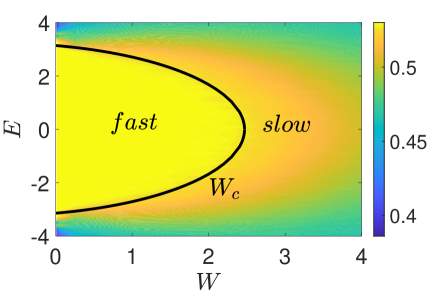
Figure 1: Phase diagram of the 2D interacting dipoles model and the color code shows the average level-spacing ratio $\langle r\rangle$, Eq. (22) characterizing the level statistics [60], evaluated for the system size $L=201$ and averaged over $1000$ realizations.

According to Eq. (17) conductance diverges logarithmically for $L\rightarrow\infty$ under the condition $c_{*}>c_{loc}$ (the fast phase), while it remains finite otherwise (the slow phase). Setting $c_{*}=c_{loc}$ one can find critical disorder separating phases.

For the dipole-dipole interaction the isotropic regime is realized only for the band center $E=0$, where the critical disorder is given by $W_{c}=\pi/\sqrt{(1+\sqrt{5})/2}\approx 2.47$. With decreasing disorder the fast phase emerges first at that energy. For the anisotropic regime realized at $E\neq 0$ the transition emerges at $c^{*}_{x}c^{*}_{y}=c_{loc}^{2}$, Eq. (21). Using the analytical results, Eq. (8), for the logarithmic growing rates $c^{*}_{x}$ and $c^{*}_{y}$ we determine the phase diagram depicted in Fig. 1, where solid lines indicate boundaries between slow and fast phases.

V Numerical results

Fast and slow phases should be distinguishable numerically and below we investigate the transition between them using exact diagonalization and considering the level statistics (Sec. V.1), fractal dimension (Sec. V.2) and transport kinetics (Sec. V.3). Since the Hamiltonian matrix is not sparse, i. e. most of its elements are different from zero, the recently developed advanced diagonalization methods of large matrices [61] are not applicable to our problem of interest and the maximum size of the system is limited to $300\times 300$. Yet our results are quite consistent with the expectations of the analytical renormalization group theory.

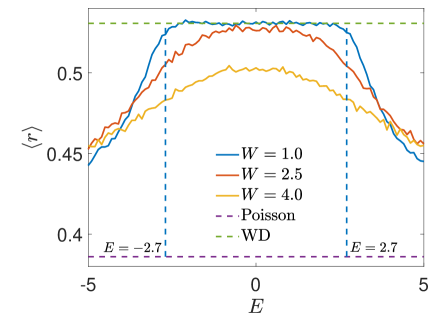
Figure 2: Level-spacing-ratio $r$-statistics vs. energy for different disorder strengths $W$. The vertical dashed lines at $E=\pm 2.7$ ($V_{0}=1$) indicate the fast phase borders for the smallest disorder strength $W=1$.

V.1 Level Statistics

Energy level statistics is different for localized and delocalized states [62]. For delocalized states it approaches the Wigner-Dyson random matrix energy level statistics due to energy level repulsion, while energies of localized states are independent of each other and can be characterized by a Poisson statistics. Usually, Wigner-Dyson level statistics indicates ergodic behavior [60; 63], see, however, Ref. .

Eigenstates in the slow phase, characterized by a finite conductance, are expected to have a fractal dimension $D$ reduced compared to a system dimension $d=2$ [11; 12]. Consequently, the level repulsion should be reduced and we do not expect Wigner - Dyson statistics and, consequently, ergodic behavior in the slow phase. However, one can expect it to appear in the fast phase similarly to the counterpart transition in $3D$ [54]. This expectation turns out to be consistent with the numerical studies reported below.

The level statistics is represented in terms of the average ratio of the minimum to maximum of adjacent energy level splittings defined as [60]

$$\langle r\rangle=\left\langle\frac{{\rm min}(\delta_{n},\delta_{n+1})}{{\rm max}(\delta_{n},\delta_{n+1})}\right\rangle,~{}\delta_{n}=E_{n+1}-E_{n},$$ (22)

where $E_{n}$ represent energies of eigenstates arranged in the ascending order. In the localized phase one has $\langle r\rangle=2\ln(2)-1\approx 0.386$, while in the delocalized, ergodic phase characterized by the Wigner-Dyson statistics $\langle r\rangle\approx 0.531$ [63].

In Fig. 2 we show the level statistics for the system of the size $L=291$ with the anisotropic dipole-dipole hopping Eq. (4) and different disorder strengths averaged over $200$ realizations.with the energy resolution $\delta E=0.1$. For the minimum disorder strength $W=1$, a substantial fraction of states with energies $|E|<2.7V_{0}$ indicated by the dashed line should belong to the fast phase (in all graphs we set $V_{0}=1$). The average level spacing ratio parameter $\langle r\rangle$ approaches the Wigner-Dyson limit $0.53$ in this domain as we expected for the fast phase. The intermediate disorder strength $W=2.5$ approximately corresponds to the last moment when the fast phase is present at $E=0$. For the strongest disorder $W=4$ all states suppose to belong to the slow phase. It is visually clear in Fig. 2 that our numerical findings are consistent with the assumption of ergodic behavior in the fast phase and its lack in the slow phase. The data for the level statistics are also presented in the phase diagram Fig. 1. They are consistent with the analytical results shown by the solid line.

V.2 Fractal dimension

We define the fractal dimension using the informational dimension $D_{1}$ [65; 66] that can be expressed in terms of the average eigenstate wavefunction Shannon entropy $\xi(L)=-\langle\sum_{i}|c_{i}|^{2}\ln(|c_{i}|^{2})\rangle$, where the amplitudes $c_{i}$ represent eigenstate coefficients of the problem in the real-coordinate basis of sites $i$ with the energy $E$ close to zero ($-0.1<E<0.1$) and averaging is performed over all such states and different realizations of random potentials. Then the informational dimension is defined as $D_{1}=d\xi/d\ln(L)$, cf. Ref. [67]. We used this definition for numerical estimates of size-dependent fractal dimension calculating the functions $\xi$ for the sequence of lengths $L_{1}$, $L_{2}$, … $L_{n}$ arranged in ascending order and then numerically differentiating them. This yields $n-1$ estimates for fractal dimensions $D_{1}(l_{k})=(\xi(L_{k+1})-\xi(L_{k}))/\ln(L_{k+1}/L_{k})$ assigned to geometrically average sizes $l_{k}=\sqrt{L_{k}L_{k+1}}$ for $k=1,2...n-1$.

Numerical results should be compared with analytical estimates for fractal dimensions obtained using the generalized theory Eq. (17) and the connection between the dimension and the system conductance. established within the non-linear sigma model in Refs. [68; 69; 70; 8]. It was shown there that the informational dimension $D_{1}$ of a two-dimensional system with a finite conductance is smaller than the system dimension $2$. The difference of dimensions is inversely proportional to the dimensionless conductance at large conductances. Consequently, the fractal (informational) dimension can be expressed as $D_{1}=2-\eta_{d}c_{loc}/C$ at $C\gg c_{loc}$. Theory suggests [70; 8] $\eta_{d}=1$ for the non-linear sigma model with a short-range hopping.

We were unable to fit the numerical data using the analytical expression with $\eta_{d}=1$ (see Appendix B), but obtained an excellent agreement between analytical and numerical results setting $\eta_{d}=1.3$ ($D_{1}=2-1.3c_{loc}/C$). In Fig. 3 we present analytical results for the fractal dimension (solid line) together with its numerical estimate for the zero energy states of the system with the hopping due to the anisotropic dipole-dipole interaction. The conductance was evaluated integrating Eq. (17) and solving numerically the resulting transcendental equation that expresses size-dependent conductance as

$$C+C_{\infty}\ln\left(1-\frac{C}{C_{\infty}}\right)=(c_{*}-c_{loc})\ln\left(\frac{L}{L_{0}}\right).$$ (23)

Here $C_{\infty}=c_{*}c_{loc}/(c_{loc}-c_{*})$ represents the infinite size limit of conductance in the slow phase $c_{*}<c_{loc}$ and $L_{0}$ is the unknown integration constant. We define this constant for each line shown in Fig. 3 minimizing the deviation of analytical ($2-1.3c_{loc}/C$) and numerical estimates of fractal dimensions. at largest sizes where the theory is most relevant.

The failure of the expression for $D_{1}$ with $\eta_{d}=1$ in the present model can be due to the long-range character of hopping.

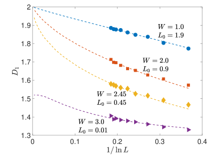
Figure 3: Finite size scaling of the fractal dimension vs. the predictions of the modified scaling theory of localization (see the text). The number of realizations is $40000$ for the minimum size $L=11$ decreasing with increasing the size to $2000$ for the maximum size $L=251$.

V.3 Transport

Finally, we consider the particle transport that is the main distinction of two phases. As we explained earlier it is expected to be superdiffusive in the fast phase and diffusive in the slow phase. For the initially localized particle its typical displacement $R$ increases with the time following a sort of diffusion law $R^{2}\propto C(R)t$ since conductance and diffusion coefficient are synonyms in two dimensions. In the fast phase a conductance $C(R)$ increases logarithmically with the size $R$ leading to a superdiffusive behavior in contrast to the linear dependence expected in the slow phase where conductance remains finite. This expectation is consistent with Ref. [11], where the behavior $R\propto t^{1/d}$ was predicted for the slow phase in a $d$- dimensional system. For $d=2$ this is equivalent to the diffusive behavior in contrast to the subdiffusive behavior for $d=3$ [11] or the superdiffusive behavior for $d=1$ [12].

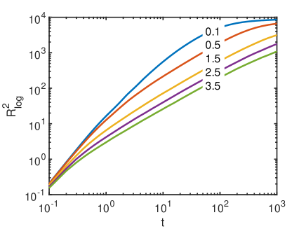
Figure 4: Time dependence of typical squared displacement at different disorder strengths $W$ indicated near each graph for the system size $L=251$, averaged over $300$ realizations.

To verify these expectations we investigate the time evolution of the state $c_{i}$ initially ($t=0$) localized in the origin $i=0$ ($c_{i}(0)=\delta_{i0}$, where $\delta_{i0}$ is the Kronecker symbol). We set a random potential in the origin to zero ($\phi_{0}=0$, see Eq. (2)) to have the average energy of the state of interest equal to zero $0$, where delocalization emerges in the maximum extent. Different strengths of random potentials were investigated including $W=0.1$, $0.5$ and $1.5$ for the fast phase, $W=2.5$ for the transition point and $W=3.5$ for the slow phase. For $W=0.1$, $0.5$ or $1.5$ the fast phase is realized for the majority of the states, except for a small fraction of the “slow” states in the tails of the spectrum that don’t affect the particle transport. The choice of a zero random potential in the origin where the particle was placed at $t=0$ reduces the contribution of slow tail states to the wavefunction evolution.

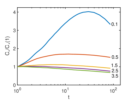
Figure 5: Time dependence of relative conductance $C_{*}/C_{*}(1)$ ($C_{*}(t)=R_{\rm log}^{2}(t)/t$) at different disorder strengths $W$ indicated on the right of each graph for the same conditions as in Fig. 4.

The particle transport has been characterized using the logarithmically average displacement $R_{\rm log}(t)$ (excluding the origin), defined as

$$\ln\left(R_{\rm log}(t)^{2}\right)=\sum_{i\neq 0}|c_{i}(t)|^{2}\ln(R_{i}^{2}).$$ (24)

We do not consider the most often used root mean square displacement because the power-law tails of the wavefunction can lead to the overestimate of the actual move. Indeed, the wavefunction asymptotic behavior $\psi(R)\propto R^{-2}$ emerges in the first order perturbation theory approach to the present problem if hopping is treated as a perturbation. Although such behavior suggests the particle localization nearby the origin $R=0$, the average squared displacement for that asymptotic behavior diverges logarithmically with the system size, while logarithmic averaging does not lead to any divergence.

The results of the calculations for $R_{\rm log}(t)^{2}$ vs. $t$ are shown in Fig. 4. Based on these results it is still difficult to characterize the transport because at very short times $t<1$, $1/W$ one has $|c_{i}(t)|\approx V_{i}t$ ($V_{i}$ is the coupling strength of the initial site and the site $i$) leading to $R_{\rm log}(t)\propto t$ , while the saturation at around the system size takes place at long times $t>100$. To focus on the relevant time domain for the superdiffusive transport we restrict our consideration to times $t_{min}<t<t_{max}$ with $t_{min}=1$ and $t_{max}=100$. The time dependence of the relative conductance $C_{*}(t)/C_{*}(1)$ ($C_{*}(t)=R_{\rm log}(t)^{2}/t$ in that time domain in shown in Fig. 5 for various disorder strengths. Relative conductance is used since we are interested in the time dependence of the diffusion coefficient (conductance) rather than its absolute value. If the transport is superdiffusive this effective conductance should increase with the time. logarithmically, saturating at long times due to a finite size effects.

According to Fig. 5 the superdiffusive transport, indeed, emerges for the weakest disorder at $W\leq 1.5$ in accord with the theoretical expectations. At short times the conductance time dependence is consistent with the expected logarithmic growing for $W=0.1$ and $W=0.5$, while for $W=1.5$ the growing domain is too narrow to make any conclusions possibly due to finite size effects. For stronger disorder the conductance slowly decreases with the time. At the transition point $W\approx 2.5$ corresponding to the zero energy, Eq. (17) predicts the superdiffusive behavior $C\propto\sqrt{\ln(L)}$, that we do not see, possibly because of dominating contributions of slow states with energies different from $0$. The reduction of the diffusion coefficient (conductance) with the time (size) for $W>1.5$ can be due to the renormalization of coupling constant occurring for the dipolar hopping and dipoles oriented within the same direction for strong disorder [71]. Although disorder is not strong, some reduction of the effective coupling constant can still take place.

VI Conclusions

We show the emergence of a superdiffusive fast phase in two-dimensional Anderson model with long-range hopping $V(r)\propto r^{-2}$, possessing the time-reversal symmetry, at sufficiently small disorder. The fast phase is characterized by delocalized, ergodic eigenstates occupying the whole space and fostering the superdiffusive transport. The complementary slow phase is non-ergodic. In this phase eigenstates are delocalized, while their fractal dimension is less than $2$. The transport there is expected to be diffusive but restricted to the maximum displacement substantially smaller than the system size.

The conductance of the system is finite in the slow phase and infinite in the fast phase. It continuously approaches infinity in the transition point in contrast to the other known localization-delocalization transitions [6; 28]. The boundary between two phases is determined analytically, which is unprecedented for Anderson localization problem with the only exception of the celebrated self-consistent theory of localization valid for the Bethe lattice [72].

Appendix A Fourier transforms of hopping amplitudes

The anisotropic dipole-dipole interaction, responsible for the hopping in the model under consideration, is defined by Eq. (4). Here we calculate numerically its Fourier transform $V(\mathbf{q})=\sum_{j}V_{ij}e^{i\mathbf{qr}_{ij}}$ needed to evaluate the zeroth order conductance, Eq. (8).

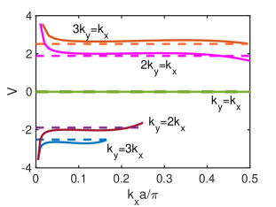
Figure 6: Comparison of analytical and numerical Fourier transforms for dipole-dipole interaction (at fixed ratios $k_{y}/k_{x}$). Numerical Fourier transform is evaluated for the system of the size $L=100$. Analytical results is shown by dashed lines and numerical results are shown by solid lines.

It turns out that dipole-dipole interaction Fourier transform can be well represented by its continuous limit given by

$$V(\mathbf{q})=V_{0}\pi\frac{-q_{x}^{2}+q_{y}^{2}}{q^{2}},$$ (25)

This approximation works reasonably well for the periodic square lattice of the size $L=100$ as illustrated in Fig. 6. It becomes exact for the system size approaching infinity since the logarithmic divergence of the zeroth order conductance emerges at $q\rightarrow 0$ corresponding to long distances. In this limit the regular correction to Eq. (25) disappears because the sum of all dipole-dipole interactions is zero.

Appendix B Connection of conductance and informational dimension.

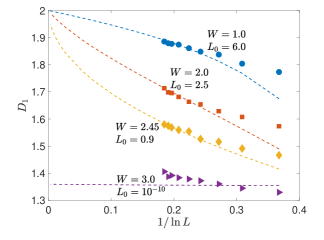
Figure 7: Comparison of the numerical estimate of eigenstate fractal dimensions with the analytical theory of Ref. [28]. The only exception is the case of $W=3$ for the present graph, where we cannot fit those data even choosing the minimum possible value of $L_{0}\rightarrow 0$, corresponding to the infinite length limit of the fractal dimension., as shown by the dashed line..

Here we show that the numerically calculated fractal dimension $D_{1}$ cannot be fitted by the analytical theory [70] predicting the dependence of this dimension on the conductance in the form $D_{1}=2-\frac{c_{loc}}{C}$ in contrast with the dependence $D_{1}=2-1.3\frac{c_{loc}}{C}$ used in the main text. We evaluated a conductance using the scaling equations derived in the present work and in Ref. [28], which can be both written in the form

$$\frac{d\ln(C)}{d\ln(L)}=\frac{c_{*}-c_{loc}}{C}+\zeta\frac{c_{*}c_{loc}}{C^{2}},$$ (26)

with $\zeta=1$ for the present work and $\zeta=1/2$ for Ref. [28].

The conductance $C$ is found integrating Eq. (26) as (see Eq. (23) in the main text)

$$C+C_{\infty}\ln\left(1-\frac{C}{C_{\infty}}\right)=(c_{*}-c_{loc})\ln\left(\frac{L}{L_{0}}\right),$$ (27)

$$C_{\infty}=\zeta\frac{c_{*}c_{loc}}{c_{loc}-c_{*}}.$$

We choose the optimum parameter $L_{0}$ in Eq. (27) as in the main text minimizing the deviation of analytical and numerical results at largest sizes.

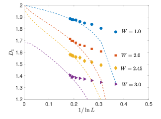
Figure 8: Comparison of the numerical estimate of eigenstate fractal dimensions with the analytical theory of the present work. We always used $L_{0}=10$.

In Figs. 7, 8 we show the comparison of the numerical results for the dimension $D_{1}$ (the numbers of realizations are as in Fig. 3) and the analytical theory $2-c_{loc}/C$ for two choices of the parameter $\zeta=1/2$ and $1$, respectively. It is clear from Figs. 7, 8 that in both cases the analytical theory does not provide an acceptable fit of the data. However, if we set $D_{1}=2-1.3c_{loc}/C$, and employ Eq. (26) with the parameter $\zeta=1$, then we get an almost perfect agreement of numerical and analytical results as reported in the main text, Fig. 3.