Nonequilibrium dynamics of suppression, revival, and loss of charge order
in a laser pumped electron-phonon system

Abstract

An electron-phonon system at commensurate filling often displays charge order (CO) in the ground state. Such a system subject to a laser pulse shows a wide variety of behaviour. A weak pulse sets up low amplitude oscillations in the order parameter, with slow decay to a slightly suppressed value. A strong pulse leads to destruction of the charge order with the order parameter showing rapid, oscillatory, decay to zero. The regime in between, separating the weak pulse CO sustained state from the strong pulse CO destroyed state, shows complex dynamics characterised by multiple, pulse strength dependent, time scales. It involves an initial rapid decay of the order parameter, followed by a low amplitude quiescent state, and the power law rise to a steady state over a timescale $\tau_{cr}$. We provide a complete characterisation of the dynamics in this nonequilibrium problem for varying electron-phonon coupling and pulse strength, examine the possibility of an effective “thermal” description of the long time state, and present results on the multiple insulator-metal transitions that show up.

I Introduction

The presence of electron-phonon (EP) interaction leads to a wide variety of effects. The most common are electron scattering leading to resistivity [1], and phonon induced electron pairing leading to superconductivity [2]. While these effects are well understood, strong EP interaction leads to the formation an electron-phonon bound state - the lattice polaron - which serves as the basic degree of freedom at strong coupling [3, 4, 5, 6]. At commensurate electron filling the polarons can order into a ‘charge ordered’ (CO) state, involving periodic modulation of the bond lengths and electron density [7, 8].

The equilibrium physics of such CO systems is well understood [9, 10, 11, 12]. Recent advances in experimental techniques allow strong perturbation of the CO state by application of a laser pulse (the ‘pump’) [13, 14, 15, 16, 17] and probe the resulting electron-phonon dynamics via time and angle resolved photoemission spectroscopy (trARPES) [18, 19, 20, 21] or resonant inelastic x-ray scattering (RIXS) [22, 23]. The dynamics in response to a weak pump pulse can be understood via linear response theory [24, 25] but the strongly perturbed system displays dynamics that requires solution of the full time dependent problem.

The pump adds excess energy to the electronic degrees of freedom. Due to the presence of EP interaction the excess energy gets redistributed among phonons and electrons. As a result, suppression and eventually melting of charge order can be observed. Such experiments have been done on 1T-TaS₂, RTe₃ and the cuprates in their charge ordered phases. Depending on the strength of the photo-excitation the following features are observed. (i) Weak photo-excitation leads to a damped periodic modulation of the electronic gap as well as the ‘electronic temperature’ [23, 26, 16]. (ii) With increasing photo-excitation one sees dynamics where the charge order vanishes at short times and then recovers slowly to a suppressed value. This is accompanied by insulator-metal-insulator transitions as a function of time [17, 29]. (iii) At strong photo-excitation the CO melts rapidly resulting in an insulator-metal transition [27, 13].

The theoretical description of melting of the charge ordered state due to photo-excitation is often phenomenologically approached via time-dependent Ginzburg-Landau theory [28, 29]. For microscopic approaches the problem is in handling widely different electron and phonon timescales at strong coupling. The associated numerics is time intensive. Methods like exact diagonalization (ED) [30] and dynamical mean field theory (DMFT) [31, 32] provide accurate results upto initial electronic timescales but cannot access the slow phonon oscillations. ED calculations are also limited by system size. The problem with a having a large number of local phonon states can be avoided by dealing with the phonons classically if the temperature and the Peierls gap is larger than the bare phonon frequency. Recent attempts have been made using Monte Carlo methods to explain the ringing in the EP system on photoexcitation [33]. The method still requires iterative diagonalization to evolve the system. Near the I-M transition the time scales of of the system diverge and with a increasing system size diagonalization even for ‘non interacting’ electrons become too costly to capture the rich dynamics of the order parameter. It is also necessary to compute the ‘two time’ Green’s function to accurately access the photoemission spectra. Our method, below, allows access to ‘long times’ at modest computational cost and captures all the key features of order parameter dynamics in a charge ordered systems.

In this paper we use a simple “mean field dynamics” (MFD) scheme to study the dynamics of the CO state in the half-filled (spinless) Holstein model in two dimensions. We set up coupled equations of motion for the expectation values of the phonon displacement operator ${\hat{x}}_{i}(t)$ and the electron bilinear ${\hat{\rho}}_{ij}(t)=c^{\dagger}_{i}(t)c_{j}(t)$ simultaneously. The equations close when one factorises the electron-phonon interaction term. Despite its apparent simplicity the method captures the effect of strong EP coupling and spatial correlations accurately. The approach goes beyond the ‘static phonon’ (or adiabatic) approximation, that has been widely used before. An approach similar to ours has been used recently to study the double exchange model [34].

We work at intermediate EP coupling (below the single polaron threshold) and probe the pulse strength $(E_{0})$ dependence of the dynamics. Our primary indicator is the phonon structure factor $S_{\bf Q}^{x}(t)$, and the charge density structure factor $S_{\bf Q}^{n}(t)$, where ${\bf Q}=(\pi/a_{0},\pi/a_{0})$ on our square lattice with spacing $a_{0}$. Our main results are the following:

• The long term state of the system shows a transition from charge ordered to charge disordered at a critical value of pulse amplitude, $E_{0}^{c}$, for fixed pulse width and frequency. At the intermediate EP coupling where we study the problem $E_{0}^{c}$ also demarcates an insulator-metal transition (IMT) in the long time electronic state.

• There are three regimes in terms of pulse strength: (i) For $E_{0}\ll E_{0}^{c}$ the structure factors $S^{x}_{\bf Q}$ and $S^{n}_{\bf Q}$ show oscillatory decay towards a suppressed long time value. (ii) For $E_{0}\rightarrow E_{0}^{c}$, the $S_{\bf Q}$ first show a drop towards zero over a timescale of few phonon oscillations, remain there for some time, and then slowly rise - recovering a finite steady state value over a timescale $\tau_{cr}$. (iii) For $E_{0}>E_{0}^{c}$, the $S_{\bf Q}$ decay monotonically to zero over a timescale that increases with $E_{0}$.

• For $E_{0}\rightarrow E_{0}^{c}$ from below, $\tau_{cr}\rightarrow\infty$, and both $S^{x}_{\bf Q}(t\rightarrow\infty)$ and $S^{n}_{\bf Q}(t\rightarrow\infty)\rightarrow 0$. For our choice of EP coupling $E_{0}^{c}\sim 0.41$.

• Probed through the density of states the electronic system remains insulating at all times when $E_{0}\ll E_{0}^{c}$, and shows an IMT when $E_{0}>E_{0}^{c}$. For $E_{0}\rightarrow E_{0}^{c}$ however it shows an insulator-metal-insulator transition as a function of time due to gap closure and revival.

• By varying the pulse strength and pulse width, at a given EP coupling, we have checked whether the long time state in our isolated system depends only on the “excess energy” $\Delta E$, imparted by the pulse. Within our method the long time state is not dependent only on $\Delta E$, suggesting the absence of thermalisation. The $E_{0}$ driven transition we observe occurs in a prethermal state.

II Model and Method

II.1 Model and evolution equation

The Holstein model is given by:

$$H~{}~{} = H_{e}+H_{ph}+H_{ep}$$ (1)

$$H_{e}~{} = \sum_{ij}t_{ij}\hat{c}_{i}^{\dagger}\hat{c}_{j}$$ (3)

$$H_{ph} = \sum_{i}(\frac{\hat{p}_{i}^{2}}{2m}+\frac{K\hat{x}_{i}^{2}}{2})$$ (4)

$$H_{ep} = -g\sum_{i}{\hat{n}}_{i}\hat{x}_{i}$$

For the $t_{ij}$ we consider nearest neighbour hopping on a square lattice. We start by writing the Heisenberg equation for ${\hat{x}}_{i}$, leading to the family below. Setting $\hbar=1$,

$${{d{\hat{x}}_{i}}\over{dt}}~{} = -i[{\hat{x}}_{i},H]={{\hat{p}}_{i}\over{m}}$$ (5)

$${{d{\hat{p}}_{i}}\over{dt}}~{} = -i[{\hat{p}}_{i},H]=-K{\hat{x}}_{i}-g{\hat{n}}_{i}$$

Now there are different options. (i) One can take an average on the left and right hand side of the equations and replace $\langle{\hat{n}}_{i}(t)\rangle$ by its expectation in the instantaneous phonon background $x_{i}(t)$. This is the ‘adiabatic evolution’ (AE) scheme, and involves iterative diagonalisation of the electron problem in ‘classical’ phonon backgrounds $\{x_{i}\}$ to compute the force on the phonons. Alternately, (ii) one can go beyond the adiabatic scheme and write an equation of motion for the ${\hat{n}}_{i}(t)$ itself, and so on, and close the hierarchy at some order. Following this route:

$${{d{\hat{n}}_{i}}\over{dt}}~{} = -i[{\hat{n}}_{i},H]=-i\sum_{mn}t_{mn}[c^{\dagger}_{i}c_{i},c^{\dagger}_{m}c_{n}]$$ (7)

$$= -i\sum_{\alpha}t_{i\alpha}(c^{\dagger}_{\alpha}c_{i}-c^{\dagger}_{i}c_{\alpha})=\sum_{\alpha}{\hat{J}}_{i\alpha}$$ (8)

$${{d{\hat{J}}_{i\alpha}}\over{dt}} = -i\sum_{mn}t_{mn}[{\hat{J}}_{i\alpha},c^{\dagger}_{m}c_{n}]-ig\sum_{j}{\hat{x}}_{j}[{\hat{J}}_{i\alpha},c^{\dagger}_{j}c_{j}]$$

Using $[c^{\dagger}_{\alpha}c_{\beta},c^{\dagger}_{m}c_{n}]=\delta_{n\alpha}c^{\dagger}_{m}c_{\beta}-\delta_{m\beta}c^{\dagger}_{\alpha}c_{n}$ and simplifying the commutators, we obtain:

$${{d{\hat{J}}_{i\alpha}}\over{dt}}=-t_{i\alpha}\sum_{mn}t_{mn}{\hat{f}}^{i\alpha}_{mn}-gt_{i\alpha}\sum_{j}{\hat{x}}_{j}{\hat{h}}^{i\alpha}_{j}$$

where the $f$ and $h$ are fermion bilinears. The first term comes purely from the hopping, the second term however involves a cross coupling between electron and phonon variables. The equations are not closed and now we need to know the dynamics of mixed objects like ${\hat{x}}_{j}{\hat{h}}^{i\alpha}_{j}$, etc. This leads to the Bogolyubov-Born-Green-Kirkwood-Yvon (BBGKY) hierarchy. We truncate the hierarchy by taking the expectation value of the LHS and RHS and approximating:

$$\langle{\hat{x}}_{j}{\hat{h}}^{i\alpha}_{j}\rangle\approx\langle{\hat{x}}_{j}\rangle\langle{\hat{h}}^{i\alpha}_{j}\rangle$$

The factorisation leads to a closed family of equations. This ‘non adiabatic evolution’ (NAE) scheme involves two processes: (i) The phonons are “driven” by $-Kx_{i}-gn_{i}$, with $n_{i}=\rho_{ii}$, where $\rho$ is the one body “density operator”, and (ii) the density operator $\rho_{ij}$ is non locally correlated and driven by the $x_{j}$.

Instead of writing a two step equation for $n_{i}$ and current we could have directly written an equation for $\rho_{ij}$, factorised it as above, and used the local component $\rho_{ii}$ in the phonon equation. The coupled equations would be:

$$m{{d^{2}{\hat{x}}_{i}}\over{dt^{2}}}~{} = -K{\hat{x}}_{i}-g{\hat{\rho}}_{ii}$$ (10)

$${{d{\hat{\rho}}_{ij}}\over{dt}}~{} = -i[{\hat{\rho}}_{ij},\tilde{H}]=-i([{\hat{\rho}}_{ij},H_{e}]+[{\hat{\rho}}_{ij},H_{ep}])$$

$$= -i[{\hat{\rho}}_{ij},H_{e}]+ig\sum_{m}[{\hat{\rho}}_{ij},{\hat{n}}_{m}]{\hat{x}}_{m}$$

From which, on taking the expectation value and factorising:

$$m{{d^{2}x_{i}}\over{dt^{2}}}~{} = -Kx_{i}-g\rho_{ii}$$ (13)

$${{d\rho_{ij}}\over{dt}} = -i\langle[{\hat{\rho}}_{ij},H_{e}]\rangle+ig\sum_{m}\langle[{\hat{\rho}}_{ij},{\hat{n}}_{m}]\rangle x_{m}$$

The two commutators can be written in terms of ${\hat{\rho}}$ itself and the $x$ is an expectation value now - a classical variable.

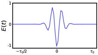
Figure 1: Laser pulse: We set the pulse width to $\tau_{p}=\tau_{0}/10$, the pulse frequency $\Omega_{p}=5\Omega_{0}$, and vary the magnitude of the electric field $E_{0}$ from $0.01-1$. We plot the time dependence of the electric field, normalized by $E_{0}$.

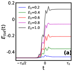
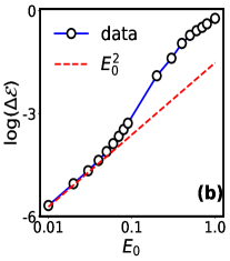
Figure 2: (a) The time dependence of the total energy $E_{tot}(t)$. The energy of the unperturbed system is $E(0)$ and pumping injects an amount of energy $\Delta E$. Since the post pulse dynamics is conservative $E_{tot}=E(0)+\Delta E$ should be constant for $t\gg\tau_{p}$. The panel confirms this and also quantifies $\Delta E(E_{0})$. (b). The dependence of $\Delta E$ on $E_{0}$, showing the ‘linear response’ regime, $\Delta E\propto E_{0}^{2}$, and beyond.

II.2 Generating the initial configuration

We consider the equilibrium system to be in its ground state. At half filling, $n=0.5$, the Holstein model with nearest neighbour hopping has a charge ordered ground state at all $g$. The CO is driven by a Fermi surface instability at small $g$ and the virtual hopping of polarons at large $g$. We obtain the reference CO state by minimising the total energy with respect to a periodic $x_{i}$ field. At the minimum, $\{x_{i}^{0}\}$, say, we use the the eigenvectors of $H\{x_{i}^{0}\}$ to compute the averages $\rho_{ij}^{0}=\langle c^{\dagger}_{i}c_{j}\rangle_{0}$.

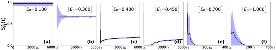
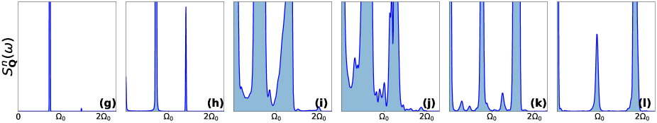
Figure 3: Overview of time dependence of the $S^{x}_{\bf Q}(t)$ at different $E_{0}$ on system size $16\times 16$. Upper row: panels (a-f) shows real time dynamics of $S^{x}_{\bf Q}(t)$. Upper row: (a)-(b): Weak pulse regime, roughly $E_{0}=0-0.35$. In this regime $x_{\bf Q}(t)$ oscillates with a single frequency and decays to a suppressed CO state. (c)-(d): Critical pulse regime, roughly $E_{0}=0.35-0.50$4. In this window $x_{\bf Q}(t)$ is rapidly suppressed, stays small for a time window, and then has a power law rise to a low amplitude long time state. (e)-(f): Strong pulse regime: for $E_{0}>0.5$ the CO gets destroyed with a few $\tau_{0}$ (not shown here) while the phonon ringing continues for a much longer time. Lower row: $S^{x}_{\bf Q}(\omega)$, the Fourier transform of $S^{x}_{\bf Q}(t)$ over the whole time range. (g)-(h): The weak pulse $S^{x}_{\bf Q}(\omega)$ has primary feature at the electronically renormalised phonon frequency $\Omega_{\bf Q}$. There is weak second harmonic, and small broadening of the lines due to mode coupling induced decay. (i)-(j): In the critical pulse regime the spectra has two broad finite frequency features, centred on a fundamental and its second harmonic, and a broad feature around $\omega=0$. (k)-(l): Shows the transform in the strong pulse window, where the real time behaviour is an oscillatory decay.

II.3 Modeling the laser pulse

We include the laser field via Peierls substituion. This leads to the time dependent hopping term:

$$H_{e}(t)=\sum_{ij}t_{ij}e^{i\phi_{ij}(t)}c_{i}^{\dagger}c_{j}$$

where $\phi_{ij}=\int_{\vec{r_{j}}}^{\vec{r_{i}}}\vec{A}(t)\cdot\vec{dr}$ and ${\vec{E}}(t)=-\frac{d\vec{A}(t)}{dt}$. For the electric field of the pulse we use the form:

$$\vec{E}(t)=\vec{E_{0}}exp[-({{t-t_{0}}\over{\tau_{p}}})^{2}]cos(\Omega_{p}t)$$

$E_{0}$ is the strength of the field, $\tau_{p}$ and the $\Omega_{p}$ are the width of the pulse and frequency of the incident wave respectively. The electric field is taken in ($\vec{x}+\vec{y}$) direction. We set $t_{0}=0$.

II.4 Parameter space

In the rest of the paper we will use $t$ as the time variable and denote the hopping $t_{ij}$ as $t_{hop}$ for nearest neighbours, and set $t_{hop}=1$.

We set $K=1$ and the oscillator mass to $m=25$ so that the local phonon frequency is $\Omega_{0}=\sqrt{K/m}=0.2$. As a result the “adiabaticity” parameter $\gamma=\Omega_{0}/t_{hop}=0.2$, small but not negligible. We measure time in units of $\tau_{0}={2\pi}/\Omega_{0}$. We focus on the half-filled case $n=0.5$.

In the adiabatic regime the energy of a polaron is $E_{p}\sim-g^{2}/{2K}$. A polaron forms when this equals the band bottom energy $-4t_{hop}$ (in two dimensions). This leads to the definition of a dimensionless EP coupling strength: $\lambda={g^{2}}/{8Kt_{hop}}$. Single polaron formation, in the adiabatic limit, corresponds to $\lambda\sim 1$. In the paper we work mainly with $\lambda=0.38$, intermediate coupling but well below the single polaron threshold.

We set $\Omega_{p}/\Omega_{0}=5$ and $\tau_{p}=\tau_{0}/10$. Having fixed $n$, $t_{hop}$, $\Omega_{0}$, $\lambda$, and the pulse parameters $\tau_{p}$ and $\Omega_{p}$, we study the response of the half filled CO state to a laser pulse for varying pulse amplitude $E_{0}$.

II.5 Numerical techniques

Most of our data are on system size N = $16\times 16$. We use the Runge-Kutta 4 (RK4) method to solve $N\times(N+2)$ coupled first order differential equations for $x_{i}$, $p_{i}$ and $\rho_{ij}$. The method scales as $\mathcal{O}(N^{2})$. Our step parameter is set to $\delta t=\tau_{0}/1500$ our total run length is $\tau_{max}=6000\tau_{0}$ at the minimum. In the critical pulse regime, where the system undergoes a transition from the CO state to a charge disordered state, simulation timescales needed to access the steady state grow rapidly. There we have used $\tau_{max}\sim 10^{5}\tau_{0}$ (on system size $12\times 12$).

II.6 Indicators

Our basic output is the time series for $x_{i}(t)$. Based on this we can compute various correlation functions of the phonon variables. We also have access to the equal time correlation $\rho_{ij}(t)=\langle c^{\dagger}_{i}(t)c_{j}(t)\rangle$, and compute the instantaneous electronic density of states (DOS) as described below.

The instantaneous structure factors related to the phonon distortions and density are, respectively:

$$S^{x}_{\bf q}(t) = {1\over N^{2}}\sum_{ij}e^{i{\bf q}.({\bf r}_{i}-{\bf r}_{j})}x_{i}(t)x_{j}(t)$$ (14)

$$S^{n}_{\bf q}(t) = {1\over N^{2}}\sum_{ij}e^{i{\bf q}.({\bf r}_{i}-{\bf r}_{j})}n_{i}(t)n_{j}(t)$$

where $n_{i}(t)=\rho_{ii}(t)$. There are the corresponding Fourier transforms to frequency, sometimes done over a finite window $t_{1}$ to $t_{2}$ (to highlight a specific dynamical feature). Such an object is

$$S^{x}_{\bf q}(\omega,t_{1},t_{2})=\int_{t_{1}}^{t_{2}}dte^{-i\omega t}S_{\bf q}^{x}(t)$$

When the transform is done over the entire time window we just call it $S^{x}_{\bf q}(\omega)$. The energy $\langle H_{e}+H_{ep}\rangle=Tr[\rho(t)H_{el}]$ where $H_{el}=t_{ij}-gx_{i}\delta_{ij}$

Finally we calculate the instantaneous electronic DOS by binning the electronic eigenvalues $\epsilon_{n}(t)$ of the electronic Hamiltonian in the background $x_{i}(t)$.

$$D(\omega,t)={1\over N}\sum_{n}\delta(\omega-\epsilon_{n}(t))$$

This is the expression one would use in the $\Omega_{0}/t_{hop}\rightarrow 0$ limit and we use it as an approximation for the DOS that should be extracted from the two time Greens function of the theory.

III Global behaviour

Before entering into the detailed characterisation of the dynamics we attempt a broad classification of regimes that occur for varying $E_{0}$. In Fig.3 we show data for $\lambda=0.38$, the results have a similar trend at other $\lambda$.

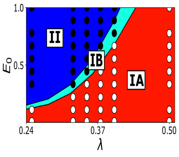
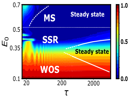
Figure 4: Top: Global phase diagram in the $\lambda-E_{0}$ plane highlighting the long time state and the rough dynamics that arises in response to a pulse. In the green region (regions I and II) the long time state has charge order. At a fixed $\lambda$ the value is monotonically suppressed with increasing $E_{0}$. In region IA, $S_{\bf Q}$ shows an oscillatory decay towards its long time CO state. In region IB, $S_{\bf Q}$ shows an initial decay to zero and then revives towards a low amplitude CO state at long times. The boundary between regions IB and II denote the quantum phase transition between CO and non CO phases. In region II, $S_{\bf Q}$ shows monotonic decay to zero with no revival. Bottom: Characterising the dynamics for various $E_{0}$ at $\lambda=0.38$. The color bar represents the strength of the normalised order parameter. We mark the “steady states” based on the data extracted from the real time dynamics.

The charge ordered state corresponds to $O(1)$ value of the Fourier transform $x_{\bf Q}=(1/N)\sum_{i}x_{i}e^{i{\bf Q}.{\bf r}_{i}}$, the order parameter of the CO state. The structure factor $S^{x}_{\bf Q}$ is simply $|x_{\bf Q}|^{2}$. The upper row in Fig.3 shows the time dependence of $S^{x}_{\bf Q}(t)$. Panels (a)-(b) are in the ‘weak pulse’ regime where we mainly see the oscillatory decay of $S^{x}_{\bf Q}(t)$ to a long time value that is suppressed with respect to the pre-pulse (equilibrium) value. We will call this response “weak oscillatory suppression” (WOS). The pre-pulse value has been set to $1$ here for convenience. Panels (c)-(d) show results in the ‘critical pulse’ regime where $S^{x}_{\bf Q}(t)$ initially drops almost to zero, stays there for some time, and then ‘revives’ heading towards a finite long time value. We call this “strong suppression and revival” (SSR) dynamics. Panels (e)-(f) show $S^{x}_{\bf Q}(t)$ in the strong pulse regime where we see a monotonic decay of the oscillation envelop to zero and there is no revival. This is simply “monotonic suppression” (MS) dynamics.

The lower row in Fig.3 shows the time Fourier transform of the corresponding upper panels, taken over the interval $0-6000\tau_{0}$. The analysis of $S^{x}_{\bf Q}(\omega)$ is best approached in terms of the behaviour of $x_{\bf Q}(t)$. If the energy added by the pulse is very small it would lead to undamped oscillation of the various normal modes, $x^{0}_{\bf q}$, of the CO state. The oscillation frequency would be $\Omega^{0}_{\bf q}$, the electronically renormalised phonon frequencies of the CO state (discussed later). The amplitude of oscillation of the modes will depend on the specific nature of the perturbation. The order parameter mode will have a response of the form $x_{\bf Q}\sim A+Bcos(\Omega^{0}_{\bf Q}t)$, where we have ignored a possible phase factor in the cosine, and $S_{\bf Q}=|x_{\bf Q}|^{2}$ will show sharp peaks at $\omega=\Omega^{0}_{\bf Q}$ and $2\Omega^{0}_{\bf Q}$ (apart from a dc component). With this as reference we now examine panels (g)-(l) in Fig.3

The response at finite but small $E_{0}$ involves some damping of the order parameter mode due anharmonicity induced coupling to other ${\bf q}$ modes. Panels (g)-(h) show the response in this regime, with $x_{\bf Q}\sim A+Be^{-t/\tau_{w}}cos(\Omega_{\bf Q}t)$. We denote the decay time in the weak pulse regime as $\tau_{w}$, and $\Omega_{\bf Q}$ is the oscillation frequency now renormalised by $E_{0}$. The damping rate $\Gamma_{w}=\tau_{w}^{-1}$ increases with $E_{0}$. However, $\tau_{w}\gg\tau_{0}$ so the damping $\Gamma_{w}\ll\Omega_{\bf Q}\sim\Omega_{0}$. As a result the spectra consists of two sharp lines at $\Omega_{\bf Q}$ and $2\Omega_{\bf Q}$. In panel (g) the oscillation amplitude is small so the feature at $2\Omega^{0}_{\bf Q}$, of $O(B^{2})$, is very weak.

For pulse strength in the critical window the general feature of $x_{\bf Q}(t)$ is rapid suppression at small times, a seeming quiescent period, and then a revival. The behaviour is accompanied by weak oscillation about the mean curve. Ignoring the sharp drop at small times, the longer time behaviour can be described roughly by $x_{\bf Q}(t)\sim Ae^{-(\tau_{cr}/t)^{\beta}}+Bcos(\Omega_{\bf Q}t)$. The ‘rise time’ to the steady state is decided by $\sim\tau_{cr}$. The mean behaviour of $S^{x}_{\bf Q}(t)$ has $e^{-(2\tau_{cr}/t)^{\beta}}$ dependence, and there are first and second harmonics of $\Omega_{\bf Q}$. Note that the $e^{-2(\tau_{cr}/t)^{\beta}}$ dependence implies a power law approach to the steady state, with $S^{x}_{\bf Q}(t)\sim 1-2(\tau_{cr}/t)^{\beta}$. The Fourier transform involves a low energy feature of width $\sim(\tau_{max}-\tau_{cr})^{-1}$ and two broadened lines around $\Omega_{\bf Q}$ and $2\Omega_{\bf Q}$.

In the strong pulse regime, (k)-(l), there appears to be stable oscillation amplitude at short times followed by a monotonic decay to zero. A simple analytic form for $x_{\bf Q}(t)$ is $A(1-e^{-(\tau_{s}/t)^{\gamma}})cos(\Omega_{\bf Q}t)$. The low frequency feature quickly vanishes as $E_{0}$ increases in this regime.

For convenience we collect together the expressions for $x_{\bf Q}(t)$ that seem to reasonably describe $S^{x}_{\bf Q}(t)=|x_{\bf Q}(t)|^{2}$ in the three regimes:

$$x_{\bf Q}(t) \sim A+Be^{-t/\tau_{w}}cos(\Omega_{\bf Q}t)~{}~{}~{}~{}~{}~{}~{}~{}~{}~{}~{}~{}~{}~{}(weak)$$ (15)

$$\sim Ae^{-(\tau_{cr}/t)^{\beta}}+Bcos(\Omega_{\bf Q}t)~{}~{}~{}~{}~{}~{}~{}~{}~{}~{}(critical)$$

$$\sim A(1-e^{-(\tau_{s}/t)^{\gamma}})cos(\Omega_{\bf Q}t)~{}~{}~{}~{}~{}~{}~{}~{}~{}~{}(strong)$$

Fig.4(a) shows the global phase diagram in the $\lambda-E_{0}$ plane, highlighting both the long time state and the rough dynamical regimes. It is based on analysis of the kind shown in Fig.3, now carried out for several $\lambda$. The bottom right region corresponds to surviving CO, while the top left corresponds to a state with CO destroyed in response to the pulse. In the ordered region regime I-A corresponds to the weak oscillatory suppression defined earlier, while I-B corresponds to strong suppression and revival. Regime II is charge disordered, where the dynamics is of monotonic suppression, and is separated from regime I-B by a nonequilibrium phase transition. A true phase transition, with $S_{\bf Q}(t\rightarrow\infty)\rightarrow 0$, as $E_{0}$ tends to some $E_{0}^{c}$, can be seen only as $L\rightarrow\infty$ and $t_{max}\rightarrow\infty$. The boundary in Fig.4(a) is drawn via extrapolation of $L$ dependent data at a few sizes, $12\times 12$ to $20\times 20$.

Fig.4(b) shows the time dependence of $S^{x}_{\bf Q}$ at $\lambda=0.38$ for different $E_{0}$. From the dynamics we classify the temporal regimes as (a) transient state: weak suppression with a decay in $S_{\bf{Q}}^{x}(t)$, (b) steady state: after initial decay the $S_{\bf{Q}}^{x}(t)$ flattens out, and (c) CO Revival: loss and slow revival of $S_{\bf{Q}}^{x}(t)$.

IV Dynamics of the CO order parameter

IV.1 Weak pulse regime

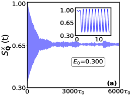
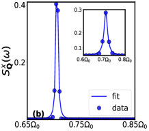
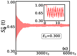
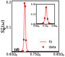
Figure 5: Weak pulse regime: (a) shows $S^{x}_{\bf Q}(t)$ with the inset highlighting the very short time behaviour. (b) Shows $S^{x}_{\bf Q}(\omega)$, obtained by Fourier transform over the entire time window, while the inset shows the transform of data over the interval $t\sim[0-15]\tau_{0}$. (c) and (d) show corresponding data for $S^{n}_{\bf Q}(t)$ and $S^{n}_{\bf Q}(\omega)$. Note the quick drop in $S^{n}_{\bf{Q}}(t)$ at very short time.

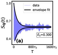
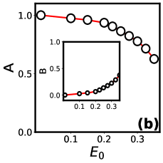
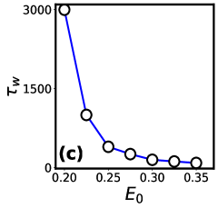
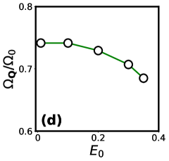
Figure 6: Characterising dynamics in the weak pulse regime. We fit the instantaneous phonon structure factor to the form given in the text. (a) Shows the fit to the envelop. (b) Shows the amplitude $A(E_{0})$, with $A^{2}$ being the steady state structure factor at the ordering wave vector. Note the sharp downward trend already apparent at $E_{0}\sim 0.35$. (c) Shows the timescale $\tau_{w}$ over which the main oscillations decay. It diverges as $E_{0}\rightarrow 0$ when the dynamics reduces to decoupled normal modes. (d) Shows the oscillation frequency $\Omega_{\bf Q}$ which shows a downward trend, akin to what one observes on raising temperature. $\Omega_{\bf Q}$ has electronic renormalisation effects built into it even at $E_{0}=0$.

Fig.5 shows in detail the phonon and charge density dynamics at a weak pulse point, $E_{0}=0.30$, at momentum ${\bf Q}$, alongwith the associated spectra. There is an initial drop, on the scale of a few $\tau_{0}$, in both $S^{x}_{\bf Q}$ and $S^{n}_{\bf Q}$, with the drop being more prominent in $S^{n}_{\bf Q}$. This is followed by an oscillatory decay to a long time state. Panels (a) and (c) show $S^{x}_{\bf Q}$ and $S^{n}_{\bf Q}$, respectively, over the whole run, while the insets show the time dependence at short times $\sim 15\tau_{0}$. As we have argued, the structure factor follows:

$$S^{x}_{\bf Q}(t)\sim[A+Be^{-t/\tau_{w}}cos(\Omega_{\bf Q}t)]^{2}$$

This simple function does not capture the oscillations (and the ‘beating pattern’) at long times but seems adequate for an overall description. Panels (b) and (d) show the respective Fourier transforms, the main panel showing the transform of the full time series and the inset showing the transform of the short time response. The panels focus on the primary harmonic and attempt to highlight the width of the line. We do not show the $2\Omega_{\bf Q}$ feature.

Panel (a) in Fig.6 shows the fit to the envelop using the fitting function above. Note that while $x_{\bf Q}$ has symmetric oscillations about amplitude $A$, $|x_{\bf Q}|^{2}$ has an asymmetry, as does the data itself. According to the fitting function, the $t\rightarrow\infty$ value of $S_{\bf Q}$ is $A^{2}$ and there will be finite frequency peaks in the spectra at frequencies $\Omega_{\bf Q}$ and $2\Omega_{\bf Q}$ with widths $\tau_{w}^{-1}$ and $2\tau_{w}^{-1}$, respectively. Panel (b) shows the $E_{0}$ dependence of $A$, which falls from $1$ at $E_{0}=0$ to $\sim 0.6$ at $E_{0}\sim 0.35$, and also $B$, which has a complementary character.

Panel (c) shows $\tau_{w}(E_{0})$, which has a remarkable decrease with increasing $E_{0}$. As $E_{0}\rightarrow 0$ the weakly perturbed lattice has only undamped normal mode oscillations, and $\tau_{w}\rightarrow\infty$. Since $\tau_{w}^{-1}$ emerges from anharmonicity, in the weak pulse limit we expect it to vary as a power $B^{\alpha}$. A plot of $log($B$)$ versus log($\tau^{-1}_{w}$) suggests that $\tau^{-1}_{w}\sim B^{2}$.

Finally, the primary oscillation frequency, $\Omega_{\bf Q}$, shows only weak $E_{0}$ dependence. The frequency for low amplitude oscillations on the CO state is given by $\Omega_{\bf Q}=\sqrt{\Omega_{0}^{2}-(g^{2}/m)\chi_{\bf Q}}$, where $\chi_{\bf Q}$ is the density response function of the CO state at momentum ${\bf Q}$. Electron-phonon coupling gives a dispersion to the phonons, and also lowers the frequency from the bare value $\Omega_{0}$. The effect of the added energy due to $E_{0}$ is to additionally reduce $\Omega_{\bf Q}$, akin to what one observes in the effect of temperature.

IV.2 Critical pulse strength regime

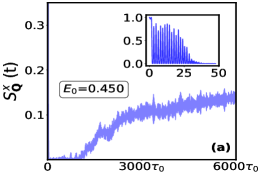
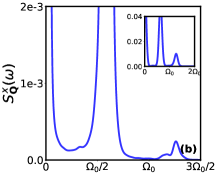
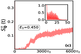
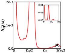
Figure 7: Critical pulse strength regime: (a) and (c) shows real time behaviour of $S_{\bf{Q}}(t)$ for the phonons and the electron density, respectively. Corresponding insets show the behaviour at short times, $t\lesssim 50\tau_{0}$. At short time the ordering amplitude in both phonons and electrons decay to zero. Then there is a very low amplitude quiescent state, followed by a ‘revival’ - rising to the long time value as $S_{\bf{Q}}(t)\sim e^{-(\tau/t)^{\beta}}$. The respective lineshapes, (b) and (d), show a peak near zero as well as broad finite frequency features at $\Omega_{\bf Q}$ and $2\Omega_{\bf Q}$.

 

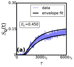
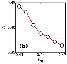
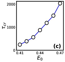
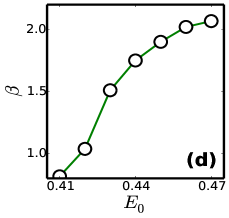
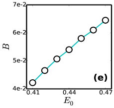
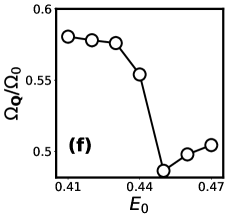
Figure 8: Characterising dynamics in the critical pulse regime. We fit $S_{x}({\bf Q},t)$ to the form $[A+Be^{-t/\tau_{w}}cos(\Omega_{\bf Q}t)]^{2}$. (a) Comparison of the envelop of the fit function with the actual data at $E_{0}=0.45$. (b) The amplitude $A$ that decides the steady state value of $S^{x}_{\bf Q}$. $A(E_{0})\rightarrow 0$ denotes the critical point. On a small lattice size we see only a limited suppression. (c) The increase in $\tau_{cr}$ by more than an order of magnitude while $E_{0}$ varies only from $0.41$ to $0.47$. The $\tau_{cr}$ should diverge at the critical point. (d) The exponent $\beta$ in the exponential rise. It varies smoothly from $\sim 1$ to $\sim 2+$ as $E_{0}$ increases. (e) The amplitude $B$ that decides the size of oscillations. Note that $B$ is one order of magnitude smaller than $A$ for the system size we have studied here. (f) The frequency $\Omega_{\bf Q}$ shows non-monotonic behaviour as it drops and rises after with $E_{0}$.

For $E_{0}\gtrsim 0.4$ the nature of $S_{\bf Q}(t)$ changes. Beyond a few cycles of oscillatory response both the phonon and charge structure factors are suppressed to roughly $\sim 1-2\%$ of their pre-pulse value, and persist in this state - with small oscillations - for a timescale that we call $\tau_{cr}$. Beyond this both $S^{x}_{\bf Q}(t)$ and $S^{n}_{\bf Q}(t)$ ‘revive’, reaching a finite but low amplitude long time state. Fig.7.(a) and (c) show the time dependence of the two structure factors at $E_{0}=0.45$, the main panels show the overall time dependence while the inset shows the initial drop that occurs over $\sim 25\tau_{0}$. Remarkably, a description of the form

$$S^{x}_{\bf Q}(t)\sim[Ae^{-(\tau_{cr}/t)^{\beta}}+Bcos(\Omega_{\bf Q}t)]^{2}$$

captures multiple features of the complex dynamics. Beyond the initial drop the function above captures the following features of the data:

• The low amplitude quiescent state, at $t\lesssim\tau_{cr}$, is described by exponentially small contribution from the first term, and small oscillations of the form $B^{2}cos^{2}(\Omega_{\bf Q}t)$, where $B\ll 1$.

• As $t$ goes beyond $\tau_{cr}$ the $A$ term makes a significant contribution, seen in the rise of the mean curve, but the oscillation amplitude also increases as $ABe^{-(\tau_{cr}/t)^{\beta}}$ due to the cross term. Since the exponential saturates for $t\gg\tau_{cr}$, the long term oscillations have a magnitude $\sim AB$ and not $B^{2}$.

• Finally, the mean value of $S^{x}_{\bf Q}$ rises as $1-(\tau_{cr}/t)^{\beta}$ at long times, a power law rather than exponential rise to the steady state.

Panels (b) and (d) show $S^{x}_{\bf Q}(\omega)$ and $S^{n}_{\bf Q}(\omega)$, respectively. There are the usual features around $\Omega_{\bf Q}$ and $2\Omega_{\bf Q}$, with the amplitude of the second term being much smaller than the first since it is proportional to $B^{2}$. There is also an interesting low energy feature, whose width we think is $\sim(\tau_{max}-\tau_{cr})^{-1}$.

Fig.8 panel (a) compares the actual data to a fit of the form assumed. We have shown only the envelop since showing the oscillations is not feasible over $6000\tau_{0}$. As we have stated the single scale $\tau_{cr}$ describes both the low amplitude quiescent state as well as the power law rise to the steady state. Panel (b) shows the amplitude $A(E_{0})$. In a later figure we will show the size dependence of this result, allowing us to extract the critical behaviour. Panel (c) shows the rapid rise of the ‘delay time’ $\tau_{cr}$ that is needed for revival of the CO state. (d) Shows the exponent $\beta$ that controls the power law approach to the steady state. (e) and (f) show the amplitude $B$, controlling the oscillations, and the primary frequency $\Omega_{\bf Q}$.

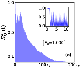
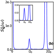
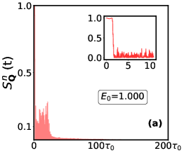
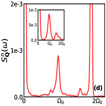
Figure 9: Strong pulse regime: (a) The relatively slow decay of $S_{x}({\bf Q})$ contrasted with (c) the rapid suppression of $S_{n}({\bf Q})$. (b) and (d) show the Fourier transforms of $S_{x}({\bf Q},t)$ and $S_{n}({\bf Q},t)$, respectively.

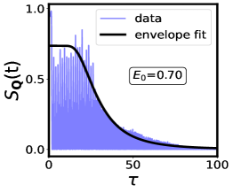
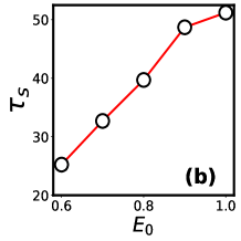
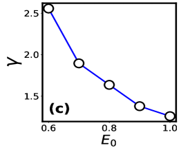
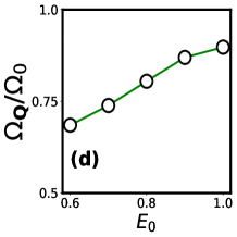
Figure 10: Strong pulse regime: fit to $S^{x}_{\bf Q}(t)$, and fitting parameters. (a) Shows the fit to the envelop, capturing both the initial flat part and the longer term decay using the same timescale $\tau_{s}$. (b) and (c) Shows monotonic increase of $\tau_{s}$ and decrease of the exponent $\gamma$ with $E_{0}$. (d) Shows the increase in the oscillation frequency towards $\Omega_{0}$ as $E_{0}$ increases. We are not showing the amplitude $A$, which stays almost constant at $A\sim 0.88$.

IV.3 Strong pulse regime

Fig.9 shows the detailed dynamics at $E_{0}=1.0$, which is in the strong pulse regime. Panel (a) shows $S^{x}_{\bf Q}(t)$, it has a modest drop one the scale of $\tau_{0}$, then a period of roughly constant oscillation for about $25\tau_{0}$, and finally a decay to zero that seems to be fit by a power law. From our fitting function:

$$S^{x}_{\bf Q}(t)\sim[A(1-e^{-(\tau_{s}/t)^{\gamma}})cos(\Omega_{\bf Q}t)]^{2}$$

the $t\ll\tau_{s}$ regime is of fixed amplitude oscillation, while for $t\gg\tau_{s}$ we get a behaviour $A^{2}(\tau_{s}/t)^{2\gamma}cos^{2}(\Omega_{\bf Q}t)$.

The responses in the charge sector, panel (c), is very different. $S^{n}_{\bf Q}$ falls sharply from $1$ to $\sim 0.15$ within $t\sim\tau_{0}$, then has roughly fixed amplitude oscillations for $t\lesssim\tau_{s}$, and then abruptly collapses. We do not see any prominent power law tail (at least at this value of $E_{0}$) unlike in $S^{x}_{\bf Q}$.

Panels (b) and (d) show the corresponding Fourier transforms. Both of these have the usual peaks at $\Omega_{\bf Q}$ and $2\Omega_{\bf Q}$, with the $2\Omega_{\bf Q}$ feature being more prominent.

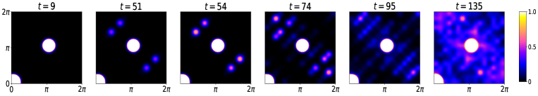
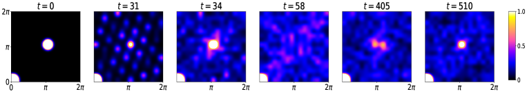
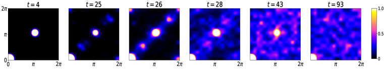
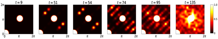
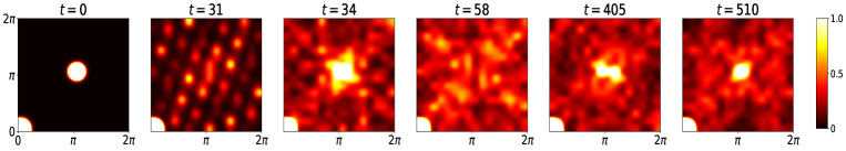
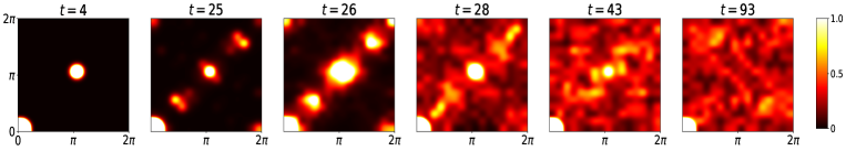
Figure 11: The full momentum dependence of $S^{x}_{\bf q}$ and $S^{n}_{\bf q}$ as a function of time in the three pulse regimes. Top three rows show $S^{x}_{\bf q}$ in the $q_{x},q_{y}$ plane for different $t$ marked on the panels. Top row: weak pulse ($E_{0}=0.2$). With increasing $t$ first the intensity of ${\bf q}$ modes along the diagonal increase and finally all ${\bf q}$ modes seem active. However the ${\bf q}={\bf Q}$ mode retains its dominant position. Middle row: critical regime ($E_{0}=0.43$). There appears to be a quick transfer of energy to ${\bf q}$ modes all over the Brillouin zone (BZ) and at $(t/\tau_{0}=58,405)$ there is no peak at ${\bf q}={\bf Q}$. There is however a recovery and in the last panel $(t/\tau_{0}=510)$ one observes high intensity at ${\bf Q}$. Bottom row: strong pulse ($E_{0}=0.7$). The timescales here are shorter than in the upper rows. The mode at ${\bf Q}$ initially transfers energy along the diagonal of the BZ, which then cascades to the rest of the BZ. By $t\sim 90\tau_{0}$ the energy has been distributed almost evenly over the BZ and there is no peak at ${\bf q}={\bf Q}$. Lower three rows show the corresponding results for $S^{n}_{\bf q}(t)$. The main difference with respect to $S^{x}_{\bf q}(t)$ is the quicker loss of order for a strong pulse.

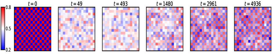
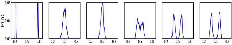
Figure 12: Top row: The spatial map of instantaneous density $n_{i}$ in the critical pulse regime for increasing time. Bottom row: the corresponding distribution of charge density $P(n,t)=(1/N)\sum_{i}\delta(n-n_{i}(t))$. At $t=0$ we have perfect checkerboard order $n_{i}$ taking values $\sim 0.2$ and $0.8$ at alternate sites. The $P(n)$ is sharply bimodal. At $t=49\tau_{0}$ the $n_{i}$ map suggests that charge modulations have essentially vanished, and $P(n)$ shows a distribution peaked around $n=0.5$. This continues at $493\tau_{0}$, and at $t=1480\tau_{0}$ we again see the emergence of charge modulations, checkerboard structures, and a bimodal tendency in $P(n)$. The last two panels show the ‘revival’ stage, with the charge density now varying roughly between $0.4$ and $0.6$. This is roughly $1/3$ the charge modulation in the $t=0$ state. The upper panel shows that the ‘phase’ of the order parameter is still well correlated, there are no obvious ‘defects’ in the structure.

Fig.10 shows the fit to the strong pulse data and the variation of the fit parameters with $E_{0}$. Panel (a) shows the fit to the actual data using the assumed functional form. Both the fixed amplitude part and the “power law” decay in $S^{x}_{\bf Q}$ are captured reasonably by the fit function. Panel (b) shows the timescale $\tau_{s}$ which increases initially with increasing $E_{0}$ (past $E_{0}^{c}$) and then tends to saturate. Panel (c) shows the exponent $\gamma$, which reduces from $\sim 2.5$ to $\sim 1.5$ as $E_{0}$ increases from $0.6$ to $1.0$. In (d) $\Omega_{\bf Q}$ increases with $E_{0}$ tending to the bare $\Omega_{0}$ (independent local oscillators) at large $E_{0}$. The amplitude $A$ is almost flat in this regime at $A=0.88$.

V Non critical modes

Till now the entire focus has been on the order parameter mode at ${\bf q}=(\pi,\pi)\equiv{\bf Q}$. While the energy of the system as a whole is conserved the energy of the lattice mode with momentum ${\bf Q}$ is not a conserved quantity. To understand the decay, or decay and revival, of this mode we need to pay attention to the other ${\bf q}$ modes to which energy is transferred via mode coupling.

While the differential equation is in terms of $x_{i}(t)$, the dynamics at weak pulse amplitude is best thought of in terms of $x_{\bf q}(t)$. The $x_{i}(t)$ is ‘driven’ by the density variable $n_{i}(t)$ which. When the $x_{i}$ and the corresponding density deviate only slightly from the ideal value we obtain normal mode vibrations at frequencies given by:

$$\Omega_{\bf q}=\sqrt{\Omega_{0}^{2}-(g^{2}/m)\Pi({\bf q})}$$

where $\Pi$ is the density response of the CO state to a change in $x$. We derive this more systematically in the Discussion section, and also show how one goes beyond the ‘independent mode’ approximation.

This undamped oscillatory behavior however works only at very weak pumping, as we have seen in Fig.3(a). It does not capture mode coupling, that leads to damping, or to the loss and revival phenomena that we observe in the critical regime. To capture these effects we need to look at the energy distribution over all ${\bf q}$ as a function of time. An analytic scheme for approaching this requires us to go beyond the linearised theory above. We will take this up in the Discussion section. For the moment we focus on the ‘activity’ in ${\bf q}$ space as revealed by our results.

       

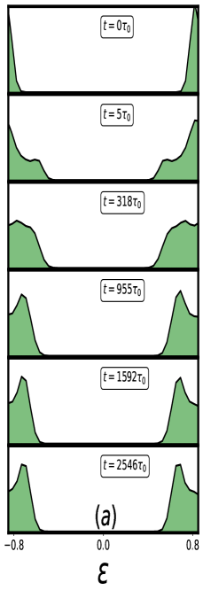
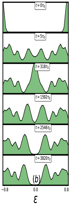
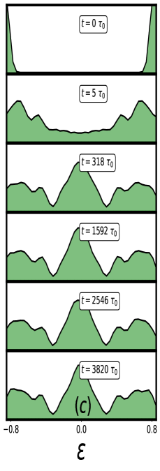
Figure 13: Electronic DOS computed on instantaneous phonon backgrounds at $\lambda=0.38$. Left column: weak pulse, $E_{0}=0.3$ showing a short time $t\sim 5\tau_{0}$ suppression of the gap and then an increase to a steady state value which is smaller than the equilibrium value. Center: critical pulse regime, $E_{0}=0.45$. Here the gap closes at $t\sim 5\tau_{0}$, stays closed (with a dip near $\omega=0$ till $t\sim 1600\tau_{0}$, and then reopens at $t\sim 2500\tau_{0}$, correlating with the loss and revival of CO. Right: strong pulse, $E_{0}=1.0$. The gap closes at $t\sim 5\tau_{0}$ and remains closed.

Fig.11 shows ${\bf q}$ maps of $S^{x}_{\bf q}$ (upper three rows) and $S^{n}_{\bf q}$ (lower three rows) as a function of time in the three pulse regimes. The principal observation from these is the following:

• At $t=0$ (pre-pulse) the only ‘bright’ feature is at ${\bf q}={\bf Q}$ and at ${\bf q}=(0,0)$ (the mean density, etc). Other modes are inert.

• At short time $\sim 10\tau_{0}$, after the pulse passes, the first additional features show up along the diagonal of the Brillouin zone (BZ). The peak at ${\bf Q}$ still remains the most prominent.

• By $t\sim 100\tau_{0}$ the disturbance has spread to the entire BZ, except at weak coupling where it is still mainly along the diagonal. In the critical and strong pulse regimes the peak at ${\bf Q}$ is hard to distinguish from the background.

• At the longest time shown in the panels, there are excitations at all ${\bf q}$ at all pulse strengths shown in the figure. However, the weak pulse panel shows a prominent peak at ${\bf Q}$, the critical pulse panel shows a weak revived peak, while the strong pulse panel shows order destroyed.

The ${\bf q}$ space picture reveals how energy is distributed over the BZ as a function of time. It does not explain whether the destruction of CO, either at intermediate time at in the critical regime or at long times in the strong pulse regime, occur due to imperfect ‘phase correlations’ between ordered domains, or due to the destruction of charge modulations itself. That requires examination of the spatial density $n_{i}$ as a function of time.

Fig.12 shows maps of $n_{i}$ in the critical window. For the EP coupling and pulse strength chosen, the main effect at intermediate time, $\sim(10^{2}-10^{3})\tau_{0}$, is the homogenisation of the charge density. We can call it ‘amplitude disordering’, in contrast to ‘phase disordering’ where modulations remain but domain structures suppress order. For $t\gtrsim 1500\tau_{0}$ the density modulations reappear, though much weaker than before, and spatially organise. At the longest time shown in this figure the $n_{i}$ field has almost perfect alternating pattern, though the modulations about $n=0.5$ are only $1/3$ of the $t=0$ value, and there is some amplitude inhomogeneity. Within our scheme, and for the lattice and parameter point that we study, the disordering and revival seems to be an amplitude effect rather than a domain interference effect.

VI Time resolved electronic spectrum

The indicators we have described till now can be probed via structure factor measurements as a function of delay time after the pulse is applied. There is also a directly measurable impact on the electronic spectrum and the associated conductivity.

Fig.13 shows the time dependence of the instantaneous DOS obtained by binning the eigenvalues $\epsilon_{n}(t)$ of the electronic Hamiltonian in the background $x_{i}(t)$. $D(\epsilon)=(1/N)\sum_{n}\delta(\epsilon-\epsilon_{n}(t))$. All data are at EP coupling $\lambda=0.38$. The left column shows data for a weak pulse, $E_{0}=0.3$, the middle column is for the critical regime $E_{0}=0.45$, and the right column is for strong pulse, $E_{0}=1.0$. At $t=0$ all the DOS have the same gap, with vanishing spectral weight over a window $\omega\sim\pm 0.7t$.

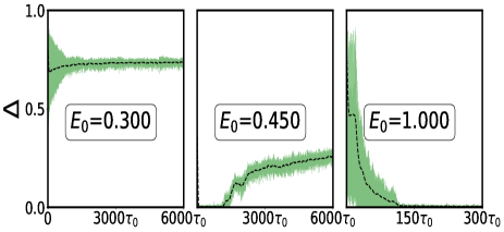
Figure 14: Gap energy ($\Delta$): The time dependence of the difference between ($N/2+1$)-th and ($N/2$)-th eigen-energy of the instantaneous Hamiltonian is plotted for three different regimes.

In the weak pulse case at very short times, $\sim 5\tau_{0}$, there is a suppression of the gap to $\sim\pm 0.5t$ and a smearing of the gap edge van Hove features. With increasing time the gap increases and the gap edge features re-form (although somewhat suppressed) and by $t\sim 2500\tau_{0}$ the gap has stabilised to $\sim\pm 0.6t$. The DOS suggests that the system remains insulating throughout.

In the critical pulse regime at $t\sim\tau_{0}$ the gap has vanished, to be repalced by a weak dip around $\epsilon=0$. At $t\sim 300\tau_{0}$, where the periodic lattice modulation is strongly suppressed, the DOS shows a prominent peak at $\epsilon=0$. Beyond this, with increasing $t$, as the lattice distortions increase and organise in the $(\pi,\pi)$ pattern again, spectral weight is lost at low energy. In the last two panels a small gap shows up in the spectrum, with width $\sim 1/3$ of the $t=0$ value. Due to the dynamics of the lattice background the electronic system shows an insulator-metal-insulator transition at this parameter point.

At strong coupling, right column, the process is monotonic. The gap closes by $t\sim 5\tau_{0}$ and for the panels at $t\gtrsim 300\tau_{0}$ we see an asymptotic metallic state with a large peak in the DOS at $\epsilon=0$. This system just shows an insulator-metal transition as a function of time.

Fig.14 quantifies the time dependence of the gap, tracked as the difference between the $N/2+1$ and $N/2$ th eigenvalue in the instantaneous spectrum. We will present optical conductivity results on this problem in the near future.

VII Discussion

In this paper we have used a conceptually simple scheme to address the dynamics in an intermediate coupling electron-phonon system, with a charge ordered ground state, subject to a laser pulse. While the static mean field theory of the CO state is elementary since it leads to a periodic potential problem, the dynamics based on mean field factorisation is technically far more complex and physically rich. In the absence of translation invariance the electronic correlator $\langle c^{\dagger}_{i}(t)c_{j}(t)\rangle$ in the background $x_{i}$ has to be evaluated by exactly solving the one body Schrodinger equation. This serves as a ‘source term’ driving the $x_{i}$ itself. The effective equation that emerges, governing the dynamics of the $x_{i}$ is highly nonlinear and spatially correlated. There are however computational and conceptual issues that we need to address.

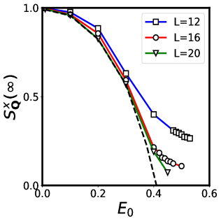
Figure 15: The dependence of $S^{x}_{\bf Q}(t\rightarrow\infty)$, obtained via the critical regime fit, on $E_{0}$ and system size $L$.

VII.1 Size effects: locating the critical point

Despite the spinless one orbital per site model for the electrons the computations are fairly expensive, scaling as $N^{2}N_{\tau}$, where $N$ is the number of lattice sites and $N_{\tau}$ is the number of integration timesteps in the interval $[0-\tau_{max}]$. Within reasonable computation time we could access $N\sim 400$ and $N_{\tau}\sim 10^{6}$ (involving about $10^{4}-10^{5}$ phonon oscillations). While this was adequate in the weak and strong pulse regimes, accessing the critical regime, where the recovery time $\tau_{cr}$ diverges as $E_{0}\rightarrow E_{0}^{c}$, was difficult. We had to extract the $t\rightarrow\infty$ value of $S^{x}_{\bf Q}$ by fitting. Fig.15 shows the result on $S^{x}_{\bf Q}(t\rightarrow\infty)$ as a function of $E_{0}$ for different $L$. It suggests a critical value $E_{0}^{c}\sim 0.41$.

VII.2 The issue of thermalisation

We are dealing with an isolated system subject to a pulse, leading to an increase in energy, and then left to evolve on its own. There is no thermal bath, however weakly coupled, and the long time property of the system will not be defined by an external temperature. Does the system thermalise internally, generating a temperature $T_{eff}$ in terms of which the long time electron and phonon state can be consistently described?

Our method made no assumption about the electrons and phonons being at some temperatures $T_{el}$ and $T_{ph}$, say, which at long times evolve towards a common $T_{eff}$. We just conserved the total energy, as shown in Fig.2(a). However, if the system did thermalise then a necessary condition is that the long time should depend on the ‘excess energy’ $\Delta E$ and not on the pulse parameters $E_{0}$, $\tau_{p}$ and $\Omega_{p}$. A preliminary check suggests that this is not the case. Keeping $\Omega_{p}$ fixed we mapped out the excess energy imparted at $\lambda=0.38$ as a function of $E_{0}$ and $\tau_{p}$. We mapped ‘equipotentials’ on the $\Delta E(E_{0},\tau_{p})$ map, and selected a set of points $\{E_{0},\tau_{p}\}_{\alpha}$, where $\alpha$ took nine values. The energy fluctuation between these points was $\sim 1-2\%$. The points are marked as $A-I$ in Fig.16(a). In Fig.16(b) we show the ‘steady state’ value of $S^{x}_{\bf Q}$ at fixed EP coupling, in response to pulses with these parameters. The $S^{x}_{\bf Q}$ vary by about $20\%$, far beyond the fluctuation we would have expected from the $\Delta E$ dispersion.

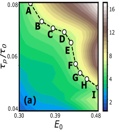
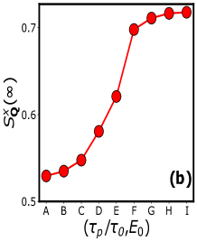
Figure 16: The left panel shows a map of the excess energy imparted to the system by a pulse of amplitude $E_{0}$ and width $\tau_{p}$, for a fixed $\Omega_{p}$ and electron-phonon coupling $\lambda$. We mark a set of points A-I at which the energy imparted to the system is the same. The right panel shows the long time lattice structure factor $S^{x}_{\bf Q}(\infty)$ after the application of pulses with these parameters. It appears that $S^{x}_{\bf Q}(\infty)$ is not a function of $\Delta E$ only - which would have led to a flat curve.

VII.3 An analytic framework

The phonons in our problem are driven by the electron density, and the electronic correlators in turn are determined by the phonon background. We can try focusing on the phonons and attempt to set up an equation for the $x_{i}$ by tracing order by order over the electrons. This is not an exact method, but a sufficiently high order expansion in $x_{i}$, and hence $x_{\bf q}$, would lead to an equation that can be compared to the time dependent Ginzburg-Landau (TDGL) equations that are used to study order parameter dynamics. Setting up such an expansion is straightforward. We have seen the lowest order version of this when discussing the non critical modes.

We rewrite the $x_{i}$ equation, at the cost of repetition:

$$m{{d^{2}{\hat{x}}_{i}}\over{dt^{2}}}=-K{\hat{x}}_{i}-g{\hat{\rho}}_{ii}$$

where $\rho_{ii}(t)=\langle c^{\dagger}_{i}(t)c_{i}(t)\rangle$. This is just the local (in space and time) projection of the Greens function $G_{ij}(t,t^{\prime})$. We can write an expansion for $G_{ij}(t,t^{\prime})$ for electrons subjected to an arbitrary time dependent $x_{i}(t)$. This takes the form:

$$G_{ii}(t,t)={\cal G}_{ii}(t,t)-g\sum_{\alpha}\int dt_{1}{\cal G}_{i\alpha}(t,t_{1})x_{\alpha}(t_{1}){\cal G}_{\alpha i}(t_{1},t)+g^{2}\sum_{\alpha\beta}\int dt_{1}dt_{2}{\cal G}_{i\alpha}(t,t_{1})x_{\alpha}(t_{1}){\cal G}_{\alpha\beta}(t_{1},t_{2})x_{\beta}(t_{2}){\cal G}_{\beta i}(t_{2},t)+O(x^{3})$$

where ${\cal G}$ is the Greens function in the reference charge ordered state. Here, $x_{i}$ is actually $\delta x_{i}=x_{i}-x_{i}^{0}$, and the effect of $x_{i}^{0}$ is incorporated in the ”bare” greens’ function ${\cal G}$. Note that while $G_{ii}(t,t)$ can depend on $i$ and $t$, the ${\cal G}$ has time and spatial translation invariance (modulo the periodic background).

To $O(x)$ the right hand side leads to a simple equation on Fourier transforming all quantities to frequency.

$${\cal G}_{i\alpha}(t,t_{1})=\int d\omega_{1}e^{i\omega_{1}(t-t_{1})}{\cal G}_{i\alpha}(\omega_{1})$$

etc. On simplification this leads to the effective linear equation of motion:

$$m\omega^{2}x_{i}(\omega)-Kx_{i}(\omega)-g^{2}\sum_{\alpha}\Pi_{i\alpha}(\omega)x_{\alpha}(\omega)=gn_{i}^{0}$$ (19)

$$(\omega^{2}-\Omega_{0}^{2}-(g^{2}/m)\Pi_{\bf q}(\omega))x_{\bf q}(\omega)=({g\over m})n^{0}_{\bf q}\delta(\omega)$$ (20)

$$\Pi_{\bf q}(\omega)=\sum_{i\alpha}\int dtdt_{1}e^{i{\bf q}.{({\bf r}_{i}-{\bf r}_{\alpha}})}e^{i\omega(t-t_{1})}{\cal G}_{i\alpha}(\omega_{1}){\cal G}_{\alpha i}(\omega-\omega_{1})$$

$n_{i}^{0}$ being the mean-field background charge density. For a given ${\bf q}$ the oscillation frequencies are roots of $(\omega^{2}-\Omega_{0}^{2}-(g^{2}/m)\Pi_{\bf q}(\omega))=0$. Note that $\Pi$ complex and if it has low frequency weight then the roots can be complex.

Going to the next surviving order, $x^{2}$ or $x^{3}$, we can write a non trivial mode coupled equation for the $x_{\bf q}(\omega)$. From this an effective damping can be extracted, as demonstrated earlier in the equilibrium CO problem [35]. The other, more complex effort, is to compare the equation to the TDGL equation. The equation here will have an integro-differential form, and would be completely deterministic in contrast to the stochastic-dissipative form assumed in the TDGL framework. We are not aware of any work following this route, and believe it can create a connection between microscopics and phenomenology, and also explore the presence or absence of thermalisation.

VII.4 Beyond $T=0$ mean field dynamics

It is usual to use the time dependent Ginzburg-Landau (TDGL) scheme to study nonequilibrium response of ordered systems. It is known that theories for $O(N)$ models, studied to leading order in $1/N$ do not show thermalisation [28]. The connection of our approach to TDGL is not obvious. Ours is overall a conservative system, with no thermal bath and no mechanism to dissipate the added energy. We do obtain a wide range of dynamical behaviour, and a pulse intensity driven phase transition, but the apparent lack of universality (in terms of the final state depending only on $\Delta E$) is puzzling. Apart from the expansion in $x_{i}$ there are two approaches that we plan to use to further probe this model.

I. We can introduce a thermal bath by explicitly coupling bath oscillators linearly to the $x_{i}$ degrees of freedom. When the bath oscillators are traced out this would lead to equations for the $x_{i}$ with an additional damping term $\gamma{\dot{x}}_{i}$ (in the Ohmic limit) and a thermal noise. One can then explore equilibriation timescales and compare with experiments.

II. We can solve the Holstein model numerically exactly on few site clusters with somewhat larger values of $\Omega_{0}/t$ to see how spatial order responds to a pulse. The local Hilbert space of the spinless Holstein model has dimension $N_{ph}\times 2$, where $N_{ph}$ is the number of phonon states retained per site. Even with $\Omega/t\sim 0.5$ we would need to retain $4-5$ phonon states per site, limiting the overall number of sites to $\sim 4-6$. While severely size limited the results can be tested against our present method on accessible sizes.

VIII Conclusions

We have studied the effect of a short laser pulse on a charge ordered system, realised in the two dimensional half filled spinless Holstein model. We work at intermediate electron-phonon coupling, at $\sim 40\%$ of the coupling needed for single polaron formation, and study the coupled dynamics of the lattice variables $(x_{i})$ and the electronic correlator $\rho_{ij}(t)=\langle c^{\dagger}_{i}(t)c_{j}(t)\rangle$ within a mean field dynamics scheme. The method is non perturbative in electron-phonon coupling and handles spatial correlations exactly. The dynamics can be categorised into three regimes with increasing pulse strength. At weak pulse strength we find a small oscillatory suppression of the order parameter to a finite long time value. At intermediate pulse strength (which we label as the critical regime) the dynamics shows strong suppression and revival of the order parameter. This involves a rapid drop of the order parameter to almost zero, where the system stays for a time $\sim\tau_{cr}$, and then a power law rise to a finite long time value. We find that $\tau_{cr}\rightarrow\infty$ and the long time value $\rightarrow 0$, as the pulse strength $E_{0}$ tends to a critical value $E_{0}^{c}$. This defines a nonequilibrium phase transition. We have established the transition by studying the system on accessible lattice size (upto $20\times 20$) and time windows. For a strong pulse the CO order parameter decays monotonically to zero. Associated with the CO order parameter behaviour is an insulator-metal-insulator transition in the critical regime, and an insulator-metal transition in the strong pulse regime. We suggest an analytic framework for addressing the results.

Acknowledgment: We acknowledge use of the HPC clusters at HRI.

References

- [1] J. M. Ziman, Electrons and phonons, Oxford University Press (2001).
- [2] See article by D. J. Scalapino in Superconductivity, Ed. R. D. Parks, Vol I, CRC Press (2019).
- [3] T. Holstein, Studies of polaron motion: Part II. The “small” polaron, Ann. Phys. (Leipzig) 8, 325 (1959).
- [4] H. Frohlich, Electrons in lattice fields, Adv. Phys. 3, 325 (1954).
- [5] E. K. H. Salje, A. S. Alexandrov, and W. Y. Liang, Polarons and Bipolarons in High Temperature Superconductors and Related Materials, Cambridge University Press (1995).
- [6] C. Franchini,, M. Reticcioli, M. Setvin, et al. Polarons in materials, Nat Rev Mater 6, 560–586 (2021).
- [7] C. P. Adams, J. W. Lynn, Y. M. Mukovskii, A. A. Arsenov, and D. A. Shulyatev, Charge Ordering and Polaron Formation in the Magnetoresistive Oxide La0.7Ca0.3MnO3, Phys. Rev. Lett. 85, 3954 (2000).
- [8] O. Bradley, G. Batrouni and R. Scalettar, Superconductivity and charge density wave order in the two-dimensional Holstein model, Phys. Rev. B. 103, 235104 (2021).
- [9] R. McKenzie, C. Hamer, and D. Murray, Quantum Monte Carlo study of the one-dimensional Holstein model of spinless fermions, Phys. Rev. B 53, 9676-9687 (1996).
- [10] S. Pradhan and G. V. Pai, Holstein-Hubbard model at half filling: A static auxiliary field study. Phys. Rev. B 92, 165124 (2015).
- [11] C. W. Chen, J. Choe, & E. Morosan, Charge density waves in strongly correlated electron systems, Rep. Prog. Phys. 79, 084505 (2016).
- [12] N. C. Costa, K. Seki, S. Yunoki & S. Sorella, Phase diagram of the two-dimensional Hubbard-Holstein model, Communications Physics, 3, 80 (2020).
- [13] Han, T., Zhou, F., Malliakas, C., Duxbury, P., Mahanti, S., Kanatzidis, M. & Chong-Yu Ruan, Exploration of metastability and hidden phases in correlated electron crystals visualized by femtosecond optical doping and electron crystallography, Science Advances, 1, e1400173 (2015).
- [14] D. Cho, S. Cheon, K. Kim, S. H. Lee, Y. H. Cho, S. W. Cheong & H. W. Yeom, Nanoscale manipulation of the Mott insulating state coupled to charge order in 1T-TaS2, Nat. Comm, 7:10453, DOI: 10.1038/ncomms10453.
- [15] M. Chávez-Cervantes, G. E. Topp, S. Aeschlimann, R. Krause, S. A. Sato, M. A. Sentef, and I. Gierz, Charge Density Wave Melting in One-Dimensional Wires with Femtosecond Subgap Excitation, Phys. Rev. Lett. 123, 036405 (2019).
- [16] Y. Zhang, X. Shi, W. You, Z. Tao, Y. Zhong, F. Kabeer, P. Maldonado, P. Oppeneer, M. Bauer, K. Rossnagel, H.Kapteyn, & M. Murnane, Coherent modulation of the electron temperature and electron-phonon couplings in a 2D material, Proceedings Of The National Academy Of Sciences, 117, 8788-8793 (2020).
- [17] J. Maklar, Y. W. Windsor, C. W. Nicholson, et al, Nonequilibrium charge-density-wave order beyond the thermal limit, Nat Commun 12, 2499 (2021).
- [18] J. Sobota, Y. He, & Z. Shen, Angle-resolved photoemission studies of quantum materials, Rev. Mod. Phys. 93, 025006 (2021).
- [19] S. Eich, A. Stange, A.V. Carr, J. Urbancic, T. Popmintchev, M. Wiesenmayer, K. Jansen, A. Ruffing, S. Jakobs, T. Rohwer, S. Hellmann, C. Chen, P. Matyba, L. Kipp, K. Rossnagel, M. Bauer, M.M. Murnane, H.C. Kapteyn, S. Mathias, M. Aeschlimann, Time- and angle-resolved photoemission spectroscopy with optimized high-harmonic pulses using frequency-doubled Ti:Sapphire lasers, Journal of Electron Spectroscopy and Related Phenomena, Volume 195, 231 (2014).
- [20] F. Schmitt, P. Kirchmann, U. Bovensiepen, R. Moore, J. Chu, D. Lu, L. Rettig, M. Wolf, I. Fisher, & Z. Shen, Ultrafast electron dynamics in the charge density wave material TbTe3, New J. Phys 13, 063022 (2011).
- [21] N. Gedik, I. Vishik, Photoemission of quantum materials, Nature Phys 13, 1029–1033 (2017).
- [22] C. Jia, K. Wohlfeld, Y. Wang, B. Moritz, & T. Devereaux, Using RIXS to Uncover Elementary Charge and Spin Excitations, Phys. Rev. X 6, 021020 (2016).
- [23] M. Mitrano, Y. Wang, Probing light-driven quantum materials with ultrafast resonant inelastic X-ray scattering, Commun Phys 3, 184 (2020).
- [24] A. Vernes, & P. Weinberger, Formally linear response theory of pump-probe experiments, Phys. Rev. B. 71, 165108 (2005).
- [25] J. Bunemann, & G. Seibold, Charge and pairing dynamics in the attractive Hubbard model: Mode coupling and the validity of linear-response theory, Phys. Rev. B. 96, 245139 (2017).
- [26] L. Rettig, J. Chu, I. Fisher, U. Bovensiepen, & M. Wolf, Coherent dynamics of the charge density wave gap in tritellurides. Faraday Discuss., 171 pp. 299-310 (2014).
- [27] S. Hellmann, M. Beye, C. Sohrt, T. Rohwer, F. Sorgenfrei, H. Redlin, M. Kallane, M. Marczynski-Buhlow, F. Hennies, M. Bauer, A. Fohlisch, L. Kipp, W. Wurth, & K. Rossnagel, Ultrafast Melting of a Charge-Density Wave in the Mott Insulator 1T-TaS2, Phys. Rev. Lett. 105, 187401 (2010).
- [28] P. Dolgirev, A. Rozhkov, A. Zong, A. Kogar, N. Gedik, & B. Fine, Amplitude dynamics of the charge density wave in : Theoretical description of pump-probe experiments, Phys. Rev. B. 101, 054203 (2020).
- [29] P. Dolgirev, M. Michael, A. Zong, N. Gedik, & E. Demler, Self-similar dynamics of order parameter fluctuations in pump-probe experiments, Phys. Rev. B. 101, 174306 (2020).
- [30] J. Okamota, Time-dependent spectral properties of a photoexcited one-dimensional ionic Hubbard model: an exact diagonalization study, New J. Phys. 21, 123040 (2019).
- [31] B. Moritz, T. P. Devereaux, and J. K. Freericks, Time-resolved photoemission of correlated electrons driven out of equilibrium, Phys. Rev. B 81, 165112 (2010).
- [32] O. P. Matveev, A. M. Shvaika, T. P. Devereaux, and J. K. Freericks, Time-domain pumping a quantum-critical charge density wave ordered material, Phys. Rev. B 94, 115167 (2016).
- [33] M. D. Petrovic, M. Weber, J. K. Freericks, Theoretical description of time-resolved photoemission in charge-density-wave materials out to long times, https://arxiv.org/abs/2203.11880
- [34] J. Luo, & G. W. Chern, Dynamics of electronically phase-separated states in the double exchange model. Phys. Rev. B. 103, 115137 (2021).
- [35] S. Bhattacharyya, S. S. Bakshi, S. Kadge, and P. Majumdar, Langevin approach to lattice dynamics in a charge-ordered polaronic system, Phys. Rev. B 99, 165150 (2019).