The impact of memory on learning sequence-to-sequence tasks

Abstract

The recent success of neural networks in natural language processing has drawn renewed attention to learning sequence-to-sequence (seq2seq) tasks. While there exists a rich literature that studies classification and regression tasks using solvable models of neural networks, seq2seq tasks have not yet been studied from this perspective. Here, we propose a simple model for a seq2seq task that has the advantage of providing explicit control over the degree of memory, or non-Markovianity, in the sequences – the stochastic switching-Ornstein-Uhlenbeck (SSOU) model. We introduce a measure of non-Markovianity to quantify the amount of memory in the sequences. For a minimal auto-regressive (AR) learning model trained on this task, we identify two learning regimes corresponding to distinct phases in the stationary state of the SSOU process. These phases emerge from the interplay between two different time scales that govern the sequence statistics. Moreover, we observe that while increasing the integration window of the AR model always improves performance, albeit with diminishing returns, increasing the non-Markovianity of the input sequences can improve or degrade its performance. Finally, we perform experiments with recurrent and convolutional neural networks that show that our observations carry over to more complicated neural network architectures.

1 Introduction

The recent success of neural networks on problems in natural language processing [1, 2, 3, 4, 5] has rekindled interest in tasks that require transforming a sequence of inputs into another sequence (seq2seq). These problems also appear in many branches of science, often in the form of time series analysis [6, 7]. Despite their ubiquity in science, there has been little work analysing learning of seq2seq tasks from a theoretical point of view in simple toy models. Meanwhile, a large body of work emanating from the statistical physics community [8, 9, 10, 11, 12] has studied the performance of simple neural networks on toy problems to develop a theory of supervised learning, where a high-dimensional input such as an image is mapped into a low-dimensional label, like its class.

An important recent insight from the study of supervised learning was the importance of data structure for the success of learning. The challenge of explaining the succes of neural networks on computer vision tasks [13, 14, 15, 16] inspired a new generation of data models that take the effective low-dimensionality of images [17] into account, such as object manifolds [18], the hidden manifold [19, 20], spiked covariates [21, 22], or low-dimensional mixture models embedded in high dimensions [23, 24, 25]. By deriving learning curves for neural networks on these and other data models [26, 27, 28, 29], the importance of data structure for the success of neural networks compared to other machine learning methods was clarified [30, 21, 23, 24].

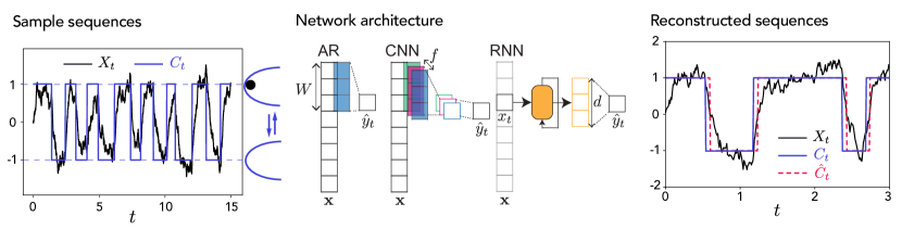
Figure 1: A flexible, minimal model for sequence-to-sequence learning tasks with varying degrees of memory along the sequence. Left: The motion of a Brownian particle (black filled circle) in a switching parabolic potential “trap” yields dynamics as given by the SSOU (stochastic switching Ornstein Uhlenbeck) model given by eq. 1. Example trajectories for sequences of the particle’s position $X_{t}$ (black line) and the trap center $C_{t}$ (blue line) as shown as a function of time $t$. The blue dashed line is set at the trap centers $C_{0}=\pm 1$. Middle: We train three types of models to reconstruct the trap positions $C_{t}$ from the particle trajectories $X_{t}$: auto-regressive models (AR) that makes predictions of the trap position based on the past $W$ observations of the particles position, as well as 1D convolutional neural networks (CNN) that acts as a set of $f$ parallel AR models with added nonlinearity in the output, and recurrent neural networks (RNN) that use feedback loops with a $d$ dimensional internal state to capture dependencies across time steps.Right: Sample reconstruction of the particle trap positions $\hat{y}_{t}$ (red dashed line) for one example input sequence ($X_{t}$, black solid line) compared with the actual hidden trap position ($C_{t}$, blue solid line). The sequence is a zoomed-in view of the sample sequence in the left panel. Parameters: $\kappa=10$, $k=1$, $D=0.5$, simulation time step $\Delta t=0.02$, AR model window size $W=2$. For this example, we used 5000 training samples, evaluated them over 5000 test samples, a mini-batch size 32 and 5 epochs.

The aforementioned breakthroughs on seq2seq tasks make it an important challenge to extend the approach of studying learning in toy models to cover the realm seq2seq tasks. What are key properties of sequences, akin to the low intrinsic dimension of images, that need to be modelled? How do these properties interact with different machine learning methods like auto-regressive models and neural networks?

Here, we make a first step in this direction by proposing to use a minimal, solvable latent variable model for time-series data that we call the stochastic switching Ornstein-Uhlenbeck process (SSOU). The input data consists of a sequence $\mathbf{x}=(x_{t})_{t=0}^{T}$, which depends on a latent, unobserved stochastic process $\mathbf{c}=(c_{t})_{t=0}^{T}$. The learning task is to reconstruct the unobserved sequence $\mathbf{c}$ from the input sequence $\mathbf{x}$, cf. fig. 1. The key data property we aim to describe and control is the memory within the input sequence $\mathbf{x}$. In the simplest scenario, the sequence $x_{t}$ is memoryless: given the value of the present token $x_{t}$, the value of the next token $x_{t+1}$ is statistically dependent solely on $x_{t}$ but not on previous tokens $x_{t^{\prime}<t}$. Such a sequence can be described by a Markov process. By tuning the dynamics of the latent process $c_{t}$, we can control the memory of the sequence, i.e. we can increase the statistical dependence of future tokens on their full history $x_{t^{\prime}<t}$ (we introduce a precise, quantitative measure for the memory below). Adding memory thus makes the process non-Markovian and allows us to model richer statistical dependencies between tokens. At the same time, the presence of memory in a process makes the mathematical analysis generally harder. Our goal is to analyse how different neural network architectures – auto-regressive (AR), convolutional (CNN), and recurrent (RNN) – handle the memory when solving the seq2seq task $\mathbf{x}\to\mathbf{c}$.

Our main contributions can be summarised as follows:

1. We introduce the stochastic switching Ornstein-Uhlenbeck (SSOU) process as a latent variable model for seq2seq tasks (section 2)

2. We introduce a measure of non-Markovianity that quantifies the memory of the sequences, and we describe how to tune the memory of the input and target sequences (section 4.1)

3. We use analytical [31] and numerical evidence to identify two regimes in the performance of the AR model in the Markovian and non-Markovian case, respectively. These regimes emerge from the interplay of two different time scales that govern the sequence statistics (section 4.2)

4. We show that the task difficulty is non-monotonic in the sequence memory for all three architectures: the task is easy with strong memory or no memory, and hardest when there is a weak amount of memory. We explain this effect using the sequence statistics (section 4.3)

5. We finally find that increasing the integration window of auto-regressive models and the kernel size of CNN improves their performance, while increasing the dimension of the hidden state of gated RNN achieves only minimal improvements (section 4.3)

Reproducibility

We provide code to sample from the SSOU model and reproduce our experiments at https://github.com/anon/nonmarkovian_learning.

2 A model for sequence-to-sequence tasks

We first describe a latent variable model for seq2seq tasks, which we call the Stochastic Switching-Ornstein-Uhlenbeck (SSOU) model. This model was introduced recently in biophysics to describe experimental recordings of the spontaneous oscillations of the tip of hair-cell bundles in the ear of the bullfrog [31]. Furthermore, a simplified variant of the model with exponential waiting times has also been fruitfully explored in the experimental context to describe the relaxation oscillations of colloidal particles in switching optical traps [32, 33].

We consider observable sequences $\mathbf{X}=(X_{t})$ which are described by a one-dimensional stochastic process whose dynamics is driven by an autonomous latent stochastic process $\mathbf{C}=(C_{t})$ and a Gaussian white noise that is independent to $C_{t}$. Here and in the following we index sequences by a time variable $t\geq 0$, and use bold letters such as $\mathbf{X}$ to denote sequences, or trajectories. A sequence of length $T$ can be sampled from the stochastic differential equation

$$X_{t+\mathrm{d}t}-X_{t}=-\kappa(X_{t}-C_{t})\mathrm{d}t+\sqrt{2D}\mathrm{d}B_{t},$$ (1)

with $t\in[0,T-1]$. Here, $\mathrm{d}B_{t}$ is the increment of the Wiener process in $[t,t+\mathrm{d}t]$, with $\langle\mathrm{d}B_{t}\rangle=0$ and $\left\langle(\mathrm{d}B_{t})(\mathrm{d}B_{t^{\prime}})\right\rangle=\delta(t-t^{\prime})\mathrm{d}t$. The angled brackets $\langle\cdot\rangle$ indicate an average over the noise process. We denote the parameters $D>0$ and $\kappa>0$ as diffusion coefficient and trap stiffness for reasons described below.

We employ this setup as a seq2seq learning task where we aim to reconstruct the hidden sequence of trap positions $\mathbf{C}$ given a sequence of particle positions $\mathbf{X}$, see fig. 1 for an illustration. The key idea in our model is to let the location of the potential $C_{t}$ alternate in a stochastic manner between the two positions $C_{0}=\{-1,1\}$. The waiting time $\tau$ spent in each of these two positions is drawn from the waiting-time distribution $\psi_{k}(\tau)$. For a generic choice of $\psi_{k}(\tau)$, the process $C_{t}$ – and hence $X_{t}$ – is non-Markovian and has a memory. Here, we use a one-parameter family of gamma distributions (defined in eq. 6 below), which allows us to quantitatively control the degree of memory in the sequence of tokens $\mathbf{C}$ in a simple manner; we discuss this in detail in section 4.1.

2.1 Physical interpretation of the SSOU model

A well-known application of eq. 1 in statistical physics is to describe the trajectories of a small particle (e.g. a colloid) in an aqueous solution undergoing Brownian motion [34] in a parabolic potential with time-dependent center $C_{t}$. Such physical model is often realized with microscopic particles immersed in water and trapped with optical tweezers [35, 32, 36]. When $\kappa=0$, the particle is driven only by the noise term $\mathrm{d}W_{t}$ and performs a one-dimensional free diffusion along the real line with diffusion coefficient $D$. By choosing $\kappa$ positive, the particle experiences a restoring force $-\kappa(X_{t}-C_{t})$ towards the instantaneous center of the potential. Such force $F(X_{t},C_{t})=-\left.\partial_{X}V(X,C)\right|_{X=X_{t},\,C=C_{t}}$ tends to confine the particle to the vicinity of the point $C_{t}$, and is therefore often called a particle trap, which is modelled by a harmonic potential centred on $C_{t}$

$$V(X_{t},C_{t})=\frac{\kappa}{2}{(X_{t}-C_{t})}^{2}.$$ (2)

This motivates the name “stiffness” for $\kappa$; the higher $\kappa$, the stronger the restoring force that confines the particle to the origin of the trap $C_{t}$. From a physical point of view, the dynamics of $X_{t}$ consists of the alternate relaxation towards the two minima of the potential between consecutive switches, cf. fig. 1.

3 Architectures and training

Auto-regressive model

We first consider the arguably simplest machine-learning model that can be trained on sequential data, an auto-regressive model of order $W$, AR($W$), see fig. 1. The output $\hat{\mathbf{y}}=(\hat{y}_{t})$ of the model for the trap position given the sequence $\mathbf{x}$ is given by

$$\hat{y}_{t}=\sigma\left(\sum_{\tau=1}^{W}w_{\tau}x_{t-\tau+1}+b\right)$$ (3)

where $\sigma(x)=1/(1+e^{-x})$ is the sigmoidal activation function, and the weights $w_{\tau}$ and the bias $b$ are trained. Its basic structure – one layer of weights followed by a non-linear activation function – makes the AR model the seq2seq analogue of the famous perceptron that has been the object of a large literature in the theory of neural networks focused on classification [8, 9, 10, 12]. Note that the window size $W\geq 1$ governs the number of tokens accessible to the model. We do not pad the input sequence, so the output sequence is shorter than the input sequence by $W-1$ steps.

Convolutional two-layer network

The auto-regressive model can also be thought of as a single layer 1D convolutional neural network [37, 38] with a single filter and a kernel of size $W$ with sigmoid activation. We also consider the natural extension of this model, CNN($W$), a 1D convolutional neural network with two layers (see fig. 1). The first layer has the same kernel size ($W$), but contains $f$ filters with rectified linear activation [39]. In the second layer, we apply another convolution with a single filter and a kernel size of 1 with sigmoid activation. In this way, we can compare a CNN and an AR model whose “integration window” are of the same length $W$. This allows us to investigate the effect of additional nonlinearities of the second layer of the CNN on the prediction error.

Recurrent neural network

We also apply a recurrent network to this task that takes $x_{t}$ as the input at step $t$, followed by a layer of Gated Recurrent Units [40] with a $d$-dimensional hidden state, followed by a fully connected layer with a single output and the sigmoid activation function (see fig. 1). We refer to this family of models by GRU($d$).

Generating the data set

We train all the models on a training set with $N$ sequences $\{\mathbf{x}^{(n)}\}_{n=1}^{N}$, which can in principle be of different lengths. To obtain a sequence, we first generate a trajectory $\mathbf{C}$ for the latent variable by choosing an initial condition at random from $C_{0}\in\{-1,1\}$ and then drawing a sequence of waiting times from the distribution $\psi_{k}(\tau)$. Using the sampled trap positions, $\mathbf{C}$, we then sample the trajectory $\mathbf{X}$ from eq. 1. Since in practice we do not have access to the full trajectory, as any experiment has a finite sampling rate, we subsample the process $X_{t}$ by taking every $s$th element of the sequence. That is, for a given sequence $\{X_{t}^{\prime}\}_{t^{\prime}=0}^{T^{\prime}}$ of length $T^{\prime}$, we construct a new sequence $\mathbf{x}={(x_{t})}_{t=1}^{T}$, where $x_{t}=X_{s\times t}$ and $T=\lfloor T^{\prime}/s\rfloor$. The subsampled sequence $\mathbf{x}$ is then used as an input sequence. We verified that the finite time step for the integration of the SDE and the subsampling preserve the statistics of the continuum description that we use to derive our theoretical results, cf. section B.2.2. For convenience, we also introduce $\mathbf{y}=(1+\mathbf{c})/2$ to shift the trap position to 0 or 1. We then use this subsampled and shifted sequence of trap positions as the target.

Training and evaluation

We train the models by minimising the mean squared loss function using Adam [41] with standard hyperparameters. For each sample sequence, the loss is defined as

$$\ell(\mathbf{y}_{t},\hat{\mathbf{y}}_{t})=\frac{1}{T-\tau_{0}}\sum_{\tau=\tau_{0}}^{T}(y_{\tau}-\hat{y}_{\tau})^{2},$$ (4)

where the offset $\tau_{0}$ in the lower limit of the sum is necessary for the AR and CNN models since their output has a different length than the input sequence. For those models we choose $\tau_{0}=W-1$. For RNN models, however, we use $\tau_{0}=1$ as the input and out sequence lengths are the same. We assess the performance of the trained models by first thresholding their outputs $\hat{y}_{t}$ at 0.5 to obtain the sequence $\hat{c}_{t}\in\{\pm 1\}$, since the location of the centre of the potential has two possible values $\pm 1$. We then use the misclassification error $\epsilon$ defined as

$$\epsilon=\frac{1}{N_{\rm{samples}}N_{\tau}}\sum_{{\rm{samples}},\tau>\tau_{h}}\delta(c_{\tau}\neq\hat{c}_{\tau}),$$ (5)

where $N_{\tau}$ is the length of the test sequence and $\delta(x)=1$ if the condition $x$ is true and it is 0 otherwise, as the figure of merit throughout this work. Unless otherwise specified, we used 50000 training samples with mini-batch size 32 to train the models, and we evaluated them over 10000 test samples. To consistently compare different models with different output lengths and to reduce the boundary effects we only consider the predictions after an initial time offset $\tau_{h}$.

4 Results

4.1 The waiting time distribution of the trap controls the memory of the sequence

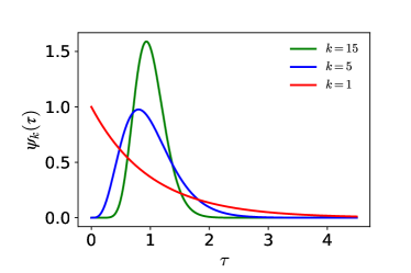
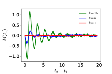
Figure 2: Quantifying the memory of non-Markovian input sequences. Left: waiting-time distribution $\psi_{k}(\tau)$ given by eq. 6 for three choices of $k$. Right: measure ${M}(t)$ (see eq. 8) associated with the parameters in the left panel, which quantifies the memory of the past time $t_{1}$ in the sequence. We obtain a memoryless sequence $X_{t}$ with ${M}(t)=0$ by choosing ${k}=1$ which creates an exponential waiting-time distribution, eq. 6 (red curves). As the value of $k$ increases, the memory becomes stronger (blue and green curves). Parameters: $D=0.5$, $\kappa=2$, $\Omega_{1}=\Omega_{2}=[0.5,1.5]$, $t_{3}-t_{2}=0.5$, by generating $N=10^{5}$ trajectories via the Euler–Maruyama method [42] with simulation time step $\Delta t=5\times 10^{-3}$.

The key data property we would like to control is the memory of the sequence $\mathbf{X}$. In our SSOU model, the memory is controlled by tuning the memory in the latent sequence $\mathbf{C}$, which in turn depends on the distribution of the waiting time $\tau$. To fix ideas, we choose gamma-distributed waiting times,

$$\psi_{k}(\tau)=\frac{1}{\tau}\frac{(\tau k)^{k}e^{-k\tau}}{\Gamma({k})},$$ (6)

where we set ${k}\geq 1$, while $\Gamma(k)=\int_{0}^{\infty}\mathrm{d}x\,x^{k-1}e^{-x}$ denotes the Gamma function. Note that for any choice of $k$, the normalization condition is $\int_{0}^{\infty}\psi_{k}(\tau)\mathrm{d}\tau=1$ and the average waiting time between two consecutive switches is $\langle\tau\rangle_{k}=\int_{0}^{\infty}\tau\psi_{k}(\tau)\,\mathrm{d}\tau=1$. We can control the shape of the distribution by changing the value of $k$: the variance of the waiting time for example is $k$-dependent, $\langle\tau^{2}\rangle_{k}-\langle\tau\rangle_{k}^{2}=1/k$ (cf. fig. 2). Furthermore, $k$ also controls the “degree of non-Markovianity” of the latent sequence $\mathbf{C}$ as follows.

For the choice ${k}=1$, the waiting-time distribution is exponential, making the process $C_{t}$ Markovian. This result, together with the fact that eq. 1 is linear, implies that the observable process $X_{t}$ is Markovian, too. Thus the probability distribution for the tokens $x_{t}$ obeys the Markov identity [34]

$$p_{1|2}(x_{t_{3}}|x_{t_{2}};x_{t_{1}})=p_{1|1}(x_{t_{3}}|x_{t_{2}}),$$ (7)

for any $t_{1}<t_{2}<t_{3}$, which represent different instants in time, and $p_{1|m}$ denotes the conditional probability density (at one time instant) with $m$ conditions (at $m$ previous time instants). Equation 7 is the mathematical expression of the intuitive argument that we gave earlier: in a Markovian process, the future state $x_{t_{3}}$ at some time $t_{3}$ given the state $x_{2}$ at some earlier time $t_{2}<t_{3}$ is conditionally independent of the previous tokens $x_{1}$ for all times $t_{1}<t_{2}$.

However, most of the sequences analysed in machine learning are non-Markovian: in written language for example, the next word does not just depend on the previous word, but instead on a large number of preceding words. We can generate non-Markovian sequences by choosing ${k}>1$. To systematically investigate the impact of sequence memory on the learning task, it is crucial to quantify the degree of non-Markovianity of the sequence for a given value of $k$ beyond the binary distinction between Markovian and non-Markovian. Yet defining a practical measure that quantifies conclusively the degree of non-Markovianity is a non-trivial task [43, 44] and subject of ongoing research mainly done in the field of open quantum systems [45, 46, 47, 48, 49].

Here, we introduce a simple quantitative measure of the degree of non-Markovianity of the input sequence motivated directly by the defining property of Markovianity given in eq. 7, which reads

$$\begin{split}M(t_{1},t_{2},t_{3})&\equiv\frac{\left\langle x_{t_{3}}|\leavevmode\nobreak\ x_{t_{2}}\!\in{\Omega_{2}},x_{t_{1}}\!\in{\Omega_{1}}\right\rangle}{\left\langle x_{t_{3}}|\leavevmode\nobreak\ x_{t_{2}}\in{\Omega_{2}}\right\rangle}-1\\ &=\frac{\int_{\mathcal{X}}x_{t_{3}}\;p_{1|2}(x_{t_{3}}|\leavevmode\nobreak\ x_{t_{2}}\!\in{\Omega_{2}},x_{t_{1}}\!\in{\Omega_{1}})\mathrm{d}x_{t_{3}}}{\int_{\mathcal{X}}x_{t_{3}}\;p_{1|1}(x_{t_{3}}|\leavevmode\nobreak\ x_{t_{2}}\!\in{\Omega_{2}})\mathrm{d}x_{t_{3}}}-1.\end{split}$$ (8)

Equation 8 involves crucially conditional expectations, where the expectation of the future system state (at time $t_{3}$) is conditioned on the present state (at time $t_{2}$), or on the present and past state (at times $t_{2}$ and $t_{1}$). We have further introduced the notion of state space regions $\Omega_{1}\subseteq\mathcal{X}$ and $\Omega_{2}\subseteq\mathcal{X}$ which are subsets of the entire state space $\mathcal{X}=\mathbb{R}$ that is accessible by the process $\mathbf{X}$. The measure ${M}$ defined in eq. 8 quantifies the drop in uncertainty about the future mean values, when knowledge about the past ($x_{t_{1}}$) is given in addition to the knowledge of the present state. Because of noise, this generally depends on how far from the past the additional data point is, $t_{2}-t_{1}$, where the decay of ${M}$ with $t_{2}-t_{1}$ quantifies the “memory decay” with increasing elapsed time. From eq. 7 it directly follows that for any Markovian process, the measure ${M}$ defined in eq. 8 vanishes at all times, whereas ${M}\neq 0$ reveals the presence of non-Markovianity in the form of memory of the past time $t_{1}$. In a stationary process, $M$ generally depends on the two time differences $t_{3}-t_{2}$ and $t_{2}-t_{1}$, and on the choices of $\Omega_{1}$ and $\Omega_{2}$. To spot the non-Markovianity, $t_{3}-t_{2}$ should be comparable to (or smaller than) the dynamical time scales of the process, which can be defined by the decay of correlation functions, which we show in fig. 6 in the appendix (namely, if $t_{3}-t_{2}$ is so large that $x_{t_{3}}$ and $x_{t_{2}}$ are fully uncorrelated, $M$ trivially vanishes even for non-Markovian processes). The choice of $\Omega_{1}$ and $\Omega_{2}$ is in principle arbitrary, but, for practical purposes, they should correspond to regions in the state space that are frequently visited.

We plot ${M}$ in fig. 2 for three different values of ${k}$ obtained from numerical simulations of the SSOU. Here, we fix $t_{2,3},\Omega_{1,2}$, and vary $t_{1}$. As expected, for a Markovian switching process with ${k}=1$, ${M}(t_{1})$ vanishes at all times $t_{1}$, while for ${k}>1$, ${M}(t_{1})$ displays non-zero values. The non-Markovianity measure $M(t_{1})$ defined in eq. 8 generally captures different facets of non-Markovianity. On the one hand, the decay with $t_{2}-t_{1}$ measures how far the memory reaches into the past. On the other hand, the magnitude of $M(t_{1})$ tells us how much the predictability of the future given the present state profits from additionally knowing the past state at time $t_{1}$. For the SSOU model, we observe in fig. 2 that increasing ${k}$ increases both the decay time and the amplitude of ${M}$, showing that that the parameter ${k}$ controls conclusively the degree of non-Markovianity. We further note that ${M}(t_{1})$ displays oscillations for ${k}>1$, reflecting the oscillatory behaviour of $\mathbf{C}$ and $\mathbf{X}$, and that ${M}(t_{1})$ always decays to zero for sufficiently large values of $t_{2}-t_{1}$, indicating the finite persistence time of the memory in the system. We note that these observations are robust with respect to the details of the non-Markovianity measure. For example, we numerically confirmed that when we change $t_{3}-t_{2}$, or $\Omega_{1,2}$, the essential features of $M$ and its dependence on $k$ remain unchanged.

In conclusion of this analysis, we can in the following simply use ${k}$ as control parameter of the degree of non-Markovianity of $\mathbf{X}$.

4.2 The performance of auto-regressive models

4.2.1 The interplay between two time scales determines prediction error

To gain some intuition, we first consider the simplest possible students, namely auto-regressive models AR(2) from eq. 3 with window size $W=2$. The student predicts the value of $c_{t}$ only using information about the present and the previous tokens $x_{t}$ and $x_{t-1}$, giving it access to the current particle position and allowing it in principle also to estimate the velocity of the particle. We show the performance of this model obtained numerically in fig. 3. The error of AR(2) varies significantly from less than $5\%$ to essentially random guessing at $50\%$ error as we vary the two time scales that influence the sequence statistics,

$$t_{\kappa}=1/\kappa\qquad\mathrm{and}\qquad t_{\rm diff}=C_{0}^{2}/2D=1/2D$$ (9)

the relaxation time and the diffusive time scale. The relaxation time $t_{\kappa}$ determines how quickly the average position of the particle is restored to the centre of the trap when the the average waiting time $\langle\tau\rangle_{k}=1$. A faster relaxation time means that the particle responds more quickly to a change in $c_{t}$, making reconstruction easier. The diffusive time scale $t_{\rm diff}$ sets the typical time that the system elapses to randomly diffuse a distance $\sim|C_{0}|$. The larger this time scale, the slower the particle moves randomly, as opposed to movement that follows the particle trap, hence improving the error.

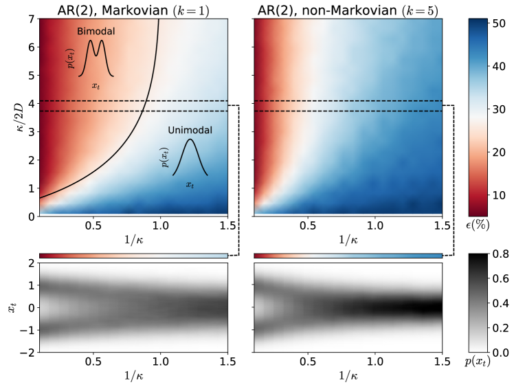
Figure 3: Performance of auto-regressive AR(2) models for Markovian and non-Markovian sequences of the SSOU model across its “learnability phase diagram”. Reconstruction error of the AR(2) model (in % of correctly predicted trap positions) for different values of the diffusive time scale $t_{\rm diff}=1/2D$ and the relaxation time $t_{\kappa}=1/\kappa$, see eq. 9. We show these “phase diagrams” for (Left) Markovian sequences ($k=1$) and for (Right) non-Markovian sequences ($k=5$). In these diagrams, the two axes represent ratios of time scales, $t_{\rm diff}/t_{\kappa}$ (vertical axis) vs $t_{\kappa}/\langle\tau\rangle_{k}=1/\kappa$ (horizontal axis), since $\langle\tau\rangle_{k}=1$ for all $k$. The bottom row depicts the distribution of particle’s position $p(x_{t})$ across the dashed line superimposed with the error heat map. The density shows a clear transition from a bimodal distribution to a unimodal one. Parameters: total simulation time for each parameter value $\tau=30$, simulation time step $\Delta t$=0.01, AR($W$) window size $W=2$, $\kappa$ varying from 0.1 to 0.6, $\tau_{h}=2$, remaining training parameters as in fig. 1.

4.2.2 A “phase diagram” for learnability

For memoryless sequences ($k=1$), we can explain this performance more quantitatively by solving for the data distribution $p(x_{t})$. Interestingly, we observe that along the “phase boundary” between unimodal and bimodal particle distribution $p(x_{t})$, the error is roughly homogeneous and approximately equal to $25\%$. The presence of two “phases” in terms of the bimodality/unimodality of the distribution $p(x_{t})$ is rationalised using recent analytical results for the loci of the phase boundary in the the case $k=1$ [31], which is given by

$$\frac{t_{\rm diff}}{t_{\kappa}}=\frac{(t_{\kappa}+1/2)\,\,{}_{1}F_{1}\left(1/2,t_{\kappa}+1/2,-t_{\rm diff}/t_{\kappa}\right)}{{}_{1}F_{1}\left(3/2,t_{\kappa}+3/2,-t_{\rm diff}/t_{\kappa}\right)}.$$ (10)

This analytical result is obtained by finding the parameter values at which the derivative of $p(x_{t})$ at $x_{t}=0$ changes sign, which corresponds to a transition between unimodal and bimodal (see section A.1 for a detailed derivation). The line separating the two phases is drawn in black in the density plot of fig. 3. In particular, we observe that reconstructing the trap position is simplified when the marginal distribution of the particle distribution $p(x_{t})$ is bimodal, i.e. when it presents two well defined peaks around the trap centres $\pm C_{0}$ (see fig. 3 top left). On the contrary, when the distribution $p(x_{t})$ is unimodal (corresponding to the case of fast relaxation times $t_{\kappa}$) the learning performance worsens as the data is not sufficiently informative about the latent state $\mathbf{C}$.

If we add memory to the sequence by choosing $k>1$, an analytical solution for the phase boundary is challenging, as it requires knowledge of the steady-state distribution of the joint system. For $k=1$, the system is Markovian and we can solve the Fokker-Planck equation for the steady-state distribution. For $k\neq 1$, the steady-state distribution is the solution of an integro-differential equation which is not solvable analytically. However, we can verify whether the same mechanism – a transition from a unimodal to a bimodal distribution for the particle distribution $p(x_{t})$ – drives the error also in the non-Markovian case by means of numerical simulations. Interestingly, when increasing the degree of memory to $k=5$ (top right of fig. 3), we find that the AR(2) model yields a larger error than for $k=1$ Markovian sequences for all the parameter values explored in the learnability phase diagram. This means that not only that AR(2) is not able to extract all the available information from the sequence, but that the task has become harder by increasing $k$. A look at the density plots for the particle distribution $p(x_{t})$ explains this finding: the transition to unimodality happens for a smaller value of the relaxation time $t_{\kappa}$ in the non-Markovian case (bottom right of fig. 3). We go into detail on how the degree of non-Markovianity makes the task harder by quantifying this transition in the probability distribution in the next section.

Further statistical characterisation of the error

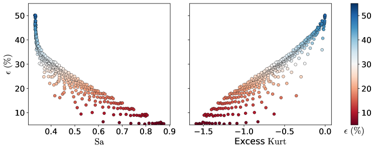
Figure 4: Statistical characterisation of the error (Left) Scatter plot of the error of several AR(2) models trained on Markovian sequences versus the Sarle coefficient, a measure of the bimodality of the distribution $p(x_{t})$, eq. 11. (Right) Scatter plot of the error of several AR(2) models trained on Markovian sequences versus the excess kurtosis, eq. 12, another measure of the bimodality of the distribution. Parameters: Similar to those used in the right panel of fig. 3

We can quantify the degree of bimodality of the particle distribution $p(x_{t})$, which drives the error of the auto-regressive model, by using the Sarle coefficient [50],

$$\mathrm{Sa}=(\sigma^{2}+1)/\mathcal{K}$$ (11)

with $\sigma$ and $\mathcal{K}$ the skewness and kurtosis of $x_{t}$, respectively. The Sarle coefficient takes values from 0 to 1 and is equal to 5/9 for the uniform distribution. Higher values may indicate bimodality. We can see a clear correlation between the Sarle coefficient and the error ($\epsilon$) of the AR(2) model from the scatter plot on the right of fig. 3. Indeed, there appears to exist an upper bound on the error in terms for the Sarle coefficient. Another measure we can compute is the excess kurtosis, which for a zero-mean random variable reads

$$\mathcal{K}_{\rm ex}=\frac{\langle x^{4}\rangle}{\left(\langle x^{2}\rangle\right)^{2}}-3,$$ (12)

where the average is over $p(x_{t})$ and we have used the fact that $\langle x_{t}\rangle=0$ by symmetry. The excess kurtosis vanishes for a Gaussian distribution and is positive or negative for non-Gaussian distributions, depending on the behaviour of the tails of the distribution (hence the name excess kurtosis). A negative value of the excess kurtosis instead indicates that the distribution is sub-Gaussian or platykurtic, i.e. having narrower tails than the Gaussian distribution. In our case, we obtain negative values of excess kurtosis whose magnitude gets larger when the distribution looks more bimodal. Furthermore, we find that the larger the more negative is the excess kurtosis, the lower is the prediction error of the AR(2) model (right of fig. 4). Taken together, this analysis shows that the prediction error becomes large when the peaks of the distribution become less distinguishable and/or in the presence of fat tails.

4.3 The interplay between sequence memory and model architecture

4.3.1 The statistical properties of the input sequence $\mathbf{x}$ with memory

We saw in fig. 3 that increasing the sequence memory by increasing the control parameter $k$ of the waiting time distribution, eq. 6, makes the problem harder: the error of the same student increased. We can understand the root of this difficulty by studying the variance of the distribution $p(x_{t},c_{t})$. Using the tools introduced by [31], we can calculate these correlations analytically for any integer $k$. As we describe in more detail in section A.2, we find that

$$\mathrm{Var}\;(x_{t}) =\langle x_{t}^{2}\rangle=\frac{D}{\kappa}\,+C_{0}^{2}\kappa\sum_{n=0}^{{k}-1}\,\frac{Q_{n}}{{k}\,q_{n}+\kappa},$$ (13a)

$$\mathrm{Cov}\;(x_{t},c_{t}) =\langle x_{t}c_{t}\rangle=1-\frac{2}{\kappa}\frac{(1+\kappa/k)^{k}-1}{(1+\kappa/k)^{k}+1},$$ (13b)

where $Q_{n}\equiv-4(1-q_{n})/({k}\,q_{n})^{2}$, and $q_{n}\equiv 1-e^{i\pi(1+2n)/{k}}$ with $n=0,\dots,{k}-1$; we recall that $\langle x_{t}\rangle=\langle c_{t}\rangle=0$. We plot both correlation functions as we vary $k$ on the right of fig. 5. First, we note that the variance of the particle distribution decreases with $k$ (red line). In other words, as we increase the memory of the sequence, the particle spends on average more time around the origin, making reconstruction harder. This is also born out by a decrease in the correlation between $x_{t}$ and $c_{t}$ (blue line). This loss in correlations is closely related to the error of the simplest reconstruction algorithm, where we estimate the particle positions $\mathbf{c}$ by thresholding the particle position, $c_{t}=\mathrm{sign}(x_{t})$, and $|C_{0}|$ identifies the amplitude of the $C_{t}$ process. As shown by a light blue line in the right panel of fig. 5, the error of this parameter-free, memoryless algorithm increases monotonically with $k$.

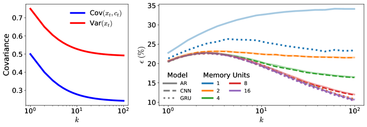
Figure 5: The impact of sequence memory on recurrent and convolutional neural networks. (Left) Analytical predictions for the covariance of the particle and trap position, eq. 13, in the non-Markovian case as a function of $k$. As we increase the non-Markovianity, correlations between $x_{t}$ and $c_{t}$ decay, complicating the reconstruction task. (Right) Prediction error $\epsilon$ for students with different architectures: auto-regressive (AR), convolutional (CNN) and gated recurrent neural network (GRU). The “memory units” of the architectures correspond to the size of the kernel ($W$) in the AR and the first layer of CNN models, and the number of units ($d$) in the hidden state of GRU models. The CNN models all have $f=10$ filters in their first layer. Parameters: Similar to fig. 3 with $\kappa=2$.

4.3.2 Increasing the integration window of autoregressive and convolutional neural networks

The existence of memory in the sequences suggests choosing student architectures that can exploit these additional statistical dependencies. We first studied the performance of AR($W$) models with varying $W$. As shown in fig. 5, we observed that for a fixed $k$ increasing $W$ generally helps with reducing the error $\epsilon$ (solid lines), so models with larger integration window can take advantage of the additional temporal correlations in the sequence and make better predictions in the large $k$ limit. For the convolutional networks described in section 3 with $f=10$ filters (dashed lines), we observe that the additional filters and non-linearities in the CNN do not help with the predictions compared to the AR($W$) models. We conclude that it is truly the size of the integration window that makes a difference on this data set and that even a simple AR model can completely take advantage of the information in a given time window.

4.3.3 Recurrent neural networks

We numerically studied the performance of a gated recurrent unit GRU($d$) [40] with hidden state size $d$, which can be thought of as a slightly more streamlined variant of the classic long short-term memory [51]. Although such an RNN reads in the input sequence one token at a time, it can exploit long-range correlations by continuously updating its internal state $\mathbf{h}\in\mathbb{R}^{d}$, cf. fig. 1. We show the test performance of GRU models with various internal state sizes $d$ in fig. 5. The GRUs display a good performance: as soon as the GRU($d$) has a hidden state with dimension $d=2$, it captures all the memory of the sequence at all $k$, achieving the limiting performance of AR($W$) models with the largest window size. Indeed, the error curves for GRUs with $d\geq 2$ all coincide. This observation, together with the limited performance gain from increasing $W$ in the AR($W$) and CNN($W$) models, suggest that the error is approaching the Bayes limit. Note that the rate of this convergence depends on $k$, since the size of the integration window required to achieve the optimal performance depends on the degree of non-Markovianity of the sequence (see fig. 5). While we focused on comparing the performance of the models here, it is important to accurately compare the computational cost of these models as well. For a detailed comparison of the complexity we refer the reader to section A.3.

4.4 The interplay between sequence memory and model architecture

Finally, we found that for all three architectures – AR, CNN and GRU – there is a peak in the reconstruction error, usually around $k\approx 5$. This peak can be understood by noting that the tokens $x_{t}$ get more concentrated around the origin as $k$ is increased, as we have shown in eq. 13. Therefore, $x_{t}$ is less correlated with $c_{t}$ in the highly non-Markovian limit. However, as the degree of non-Markovianity is increased through increasing $k$, the history of the tokens position $x_{t}$ can help with predicting the trap’s position $c_{t}$ more accurately. The trade-off between these two phenomena is evident in the non-monotonic dependency of the error as a function of $k$ for models with larger integration window in fig. 5. For small $k$, the correlation between different times in the sequence is not strong enough to compensate the loss of information about the trap’s position in the signal, but for larger $k$ the trap’s position is more regular and the history of $x_{t}$ can be used to infer the $c_{t}$ more efficiently.

5 Concluding perspectives

We have applied the stochastically switching Ornstein-Uhlenbeck process (SSOU) to model seq2seq machine learning tasks. This model gives us precise control over the memory of the generated sequences, which we used to study the interaction between this memory and various neural network architectures trained on this data, ranging from simple auto-regressive models to convolutional and recurrent neural networks. We found that the accuracy of these models is governed by the interaction of the different time scales of the data, and we discovered an intriguing, non-trivial interplay between the architecture of the students and the sequence which leads to non-monotonic error curves.

An important limitation of the SSOU model considered here is that it only allows one to study correlations that decay exponentially fast. As a next step it would be interesting to explicitly consider the impact of long-range memory in the data sequence. This could be implemented in the SSOU model e.g. by choosing a long-ranged waiting time distribution, such as a power law. Another limitation concerns the linearity of the model analysed here. We speculate that a nonlinear model could provide insights into the different ways AR and CNN utilise the data. In our model, one could implement a tunable nonlinearity by considering e.g. a double-well potential with increasing amplitude of the potential barrier. Similarly, to enrich the statistical dependencies within the sequence, one could generate non-symmetric sequences with respect to a $x\to-x$ sign inversion, by implementing two different waiting-time distributions. It would also be interesting to analyse the impact of sequence memory on the dynamics of simple RNN models [52, 53], such as those with low-rank connectivity [54, 55].

Another exciting avenue would be to apply neural networks to noisy non-Markovian signals extracted from experiments in physical or biological systems [56, 57, 58, 59, 60, 61, 62]. Examples include the recent application of the SSOU to infer the mitigation of the effects of non-Markovian noise [63, 64] and the underlying heat dissipation of spontaneous oscillations of the hair-cell bundles in the ear of the bullfrog [31]. Applying our techniques to such a biological system could be fruitful to decipher the hidden mechanisms and statistics of switching in hearing and infer thermodynamic quantities beyond energy dissipation.

Appendix A Analytical details

A.1 Details on the calculation of the phase diagram

As anticipated in section 4.1, the process $C_{t}$ becomes Markovian in the case of exponentially distributed waiting time distribution; in our units this coincides with $\psi_{k=1}(\tau)=e^{-\tau}$. For this simple case, one can characterise analytically the mono–bistable transition of the stationary density $p(x_{t})$. This can be done by looking at the behaviour of $p(x_{t})$ at the origin: if $x_{t}=0$ is a point of maximum, $p(x_{t})$ is unimodal, bimodal otherwise. We report from [31] the explicit expression of $p(x_{t})$, which reads

$$p(x_{t})=\frac{1}{\sqrt{\pi}}\frac{\Gamma\left(\zeta+\frac{1}{2}\right)}{\Gamma\left(\zeta\right)}\int_{-1}^{+1}\mathrm{d}z\,\frac{e^{-\chi(x_{t}-z)^{2}}}{\sqrt{\pi/\chi}}(1-z^{2})^{\zeta-1},$$ (A.1)

where we have set $C_{0}=1$, and we have defined the dimensionless parameters $\zeta=t_{\kappa}/\langle\tau\rangle_{k}=1/\kappa$ and $\chi=t_{\rm diff}/t_{\kappa}=\kappa/(2D)$. One finds that $x_{t}=0$ is an extremum point for $p(x_{t})$, coinciding with the condition $p^{\prime}(0)=0$. The nature of $x_{t}=0$ is understood by looking at the second derivative of $p(x_{t})$, that is

$$p^{\prime\prime}(0)=\frac{2}{\sqrt{\pi/\chi^{3}}}\left[\frac{\chi}{\zeta+1/2}\,\,{}_{1}F_{1}\left(\frac{3}{2},\zeta+\frac{3}{2},-\chi\right)-{}_{1}F_{1}\left(\frac{1}{2},\zeta+\frac{1}{2},-\chi\right)\right],$$ (A.2)

where ${}_{1}F_{1}$ denotes the confluent hypergeometric function. The mono-bimodal transition occurs upon crossing the critical value $\chi^{*}$ satisfying the condition $p^{\prime\prime}(0)=0$, or equivalently, eq. (10). For $\chi<\chi^{*}$, the second derivative $p^{\prime\prime}(0)$ is negative and $p(x)$ is unimodal, while it is bimodal otherwise.

When waiting times do not follow an exponential distribution, the system ceases to be Markovian. As far as our understanding goes, it becomes impossible to precisely compute the stationary probability density $p(x_{t})$. Nevertheless, in the upcoming section, we will demonstrate that when $k>1$, it remains feasible to derive a complete expression for the two-point time correlators.

A.2 Computation of the correlation functions in the non-Markovian case

In this section, we report the analytical expression for the (stationary) auto-correlation function $\mathcal{C}_{X}(t)$ of the process $X_{t}$ in eq. (1), and its Fourier transform, i.e., the power spectral density (PSD) $S_{X}(\omega)$. For Gamma-distributed waiting-time $\psi_{k}(\tau)$ as given in eq. (6), the PSD $S_{X}(\omega)$ of the process $X_{t}$ is given by [31]

$$S_{X}(\omega)=\frac{2D+\kappa^{2}S_{C}(\omega)}{\kappa^{2}+\omega^{2}},$$ (A.3)

where $S_{C}(\omega)$ denotes the PSD of the process $C_{t}$, whose explicit expression reads

$$S_{C}(\omega)=\frac{4C_{0}^{2}}{\omega^{2}}\frac{R^{2}(\omega)-1}{R^{2}(\omega)+1+2R(\omega)\cos\phi(\omega)},$$ (A.4)

with $R(\omega)=\left[1+(\omega/{k})^{2}\right]^{{k}/2}$, and $\phi(\omega)={k}\arctan(\omega/{k})$. According to the Wiener-Khinchin theorem [34], the inverse Fourier transform of $S_{C}(\omega)$ and $S_{X}(\omega)$ coincides with the auto-correlation functions $\mathcal{C}_{C}(t)\equiv\lim_{\tau\to\infty}\langle C_{t+\tau}\,C_{\tau}\rangle$ and $\mathcal{C}_{X}(t)\equiv\lim_{\tau\to\infty}\langle X_{t+\tau}\,X_{\tau}\rangle$. In the case of integer ${k}$, their expressions can be calculated explicitly according to

$$\mathcal{C}_{C}(t)=C_{0}^{2}\sum_{n=0}^{{k}-1}Q_{n}\,e^{-t\,{k}\,q_{n}},$$ (A.5)

$$\mathcal{C}_{X}(t)=\frac{D}{\kappa}\,e^{-\kappa\,t}+C_{0}^{2}\,\kappa\sum_{n=0}^{{k}-1}Q_{n}\,\frac{{k}\,q_{n}\,e^{-\kappa\,t}-\kappa\,e^{-{k}\,q_{n}\,t}}{({k}\,q_{n})^{2}-\kappa^{2}},$$ (A.6)

where $Q_{n}\equiv-4(1-q_{n})/({k}\,q_{n})^{2}$, and $q_{n}\equiv 1-e^{i\pi(1+2n)/{k}}$ with $n=0,\dots,{k}-1$; in fig. 6, we compare eq. (A.6) with the numerical estimate of $\mathcal{C}_{X}$ for three different choices of $k$. Note that the value of the sum $\sum_{n=0}^{{k}-1}Q_{n}=1$ implies the correct initial condition $C_{c}(0)=C_{0}^{2}$. Moreover, one can deduce the stationary expression of the stationary variance $\langle x_{t}^{2}\rangle$ of the process $X_{t}$ from the initial value $\mathcal{C}_{X}(0)$. We conclude this section by reporting the value of the covariance $\langle x_{t}c_{t}\rangle$, which we derive here using similar methods as those in ref. [31], and is given by

$$\langle x_{t}c_{t}\rangle=1-\frac{2}{\kappa}\frac{(1+\kappa/k)^{k}-1}{(1+\kappa/k)^{k}+1}.$$ (A.7)

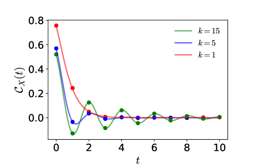
Figure 6: Autocorrelation function of the process $C_{t}$. We compare the analytical formula of $\mathcal{C}_{X}(t)$ in eq. (A.5) (solid line) with its numerical prediction (circles), calculated by generating $N=5\times 10^{4}$ trajectories via Euler–Maruyama method with $\Delta t=0.01$, $\kappa=2$, $D=0.5$ and various values of $k$.

A.3 Complexity of the models

In this section we analyse the size and computational complexity of the models used in this study. We note that the exact complexity depends on the specific implementation of the models. Therefore, we first analyse the scaling of the model complexity with respect to the number of model’s memory units and then characterise the number of floating-point operations (FLOPs) in our particular implementation.

In this scaling analysis we do not consider the scaling with the sequence size it is the same for all of the models. The auto-regressive (AR) models we examine feature a 1D kernel of size $W$. Both the model’s parameter count and computational complexity for its forward pass increase linearly with $W$. Similarly, 1D convolutional neural networks (CNN) comprise $f$ kernels of size $W$. For these models, the number of parameters and computational cost scale primarily as $Wf$. The gated recurrent units (GRU) have a hidden state of size $d$. The number of parameters and the computational cost of these model scale with $d^{2}$.

We employ software profiling to accurately compare the size and computational cost of the models used to produce fig. 5. As demonstrated in fig. 7, our analysis agrees with the numerical results. The AR models exhibit the smallest size and computational cost, followed by CNNs, and finally RNNs. Additionally, our simple analysis correctly predicts linear scaling of cost with the number of parameters.

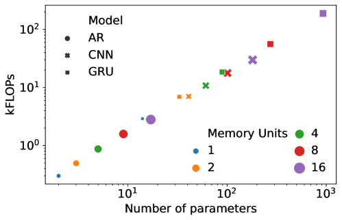
Figure 7: Complexity of the models. We analyze the size and computational complexity of the models used to generate fig. 5, i.e., auto-regressive (AR), convolutional (CNN), and gated recurrent neural network (GRU) architectures. Computational complexity is measured in terms of floating-point operations (FLOPs). The ’memory units’ in these architectures correspond to the kernel size ($W$) in AR and the GRU hidden state size ($d$). Notably, all CNN models employ 10 filters in their first layer.

Appendix B Additional experimental results

We use a fixed number of 40 epochs and do not perform any hyperparameter tuning (with the exception of the GRU(1) model as detailed in Appendix B) as the models are rather simple and varying these parameters have negligible effects on the results.

B.1 Additional details on creating the figures

In this section, we provide additional details on the generation of some of the figures of the main text.

Figure 3

The parameter sweep in the top left and top right panels was done by inspecting the intervals $\kappa\in[2/3,10]$ and $D\in[1/21,50]$ in a regular grid of size 20$\times$20. We used a finite-sample estimate for Sarle’s coefficient given by $(\sigma^{2}+1)/(3+\omega\mathcal{K})$, with $\sigma$ the skewness and $\mathcal{K}$ the kurtosis of the sequence $\mathbf{X}$, and $\omega=(T-1)^{2}/(T-2)(T-3)$ and $T=\tau/\Delta t=3\times 10^{3}$.

B.2 Ensuring the consistency between continuous-time theory and sampled sequences

Here we discuss how we ensured that our theory that is based on the continuous-time description of the stochastic processes $X_{t}$ and $C_{t}$ (cf. section 2) and the sequences we find into the machine learning models are consistent. If the sequence is sampled with a very small time step, the student almost never sees a jump of the trap, and effectively samples from an (equilibrium) distribution in one trap. On the other hand, in the limit of very large time steps, the temporal correlations in the sequence is not visible, e.g., recall that the non-Markovianity parameter eventually decays to zero for infinitely large time differences. Thus, it is crucial to sample with a time step that is smaller but comparable to the characteristic time scales of the data sequence. In practice, one would thus need to estimate those time scales in a preceding data analysis step, before feeding the data into the network. For this purpose, a suitable method is to compute the autocorrelation function of the input sequence data which reveals the time scales. For the SSOU model, we provide the analytical expression for the correlation function in eq. 13. For the SSOU, the characteristic time scales are given by the oscillation period and the decay time of the autocorrelation function, which are of order of magnitude 1 for our parameter choice (see fig. 6 ).

B.2.1 Correlations function and integration time step

To generate trajectories with correct statistics we vary the time differences $\Delta t$, which corresponds to the discrete version of $\mathrm{d}t$ in numerically integrating eq. (1). We find that $\Delta t=0.005$ reproduces the correct statistics in fig. 6.

B.2.2 The role of subsampling

As mentioned earlier the trajectories are first generated by numerically integrating eq. (1) by choosing a sufficiently small $\mathrm{d}t$ such that the statistical properties of the trajectories match their theoretical values, which we verified by checking the correlation functions estimated analytically match our theoretical result (see fig. 6).

As we discuss in the main text, we subsample the full trajectories before training the machine learning models. This subsampling also simplifies the optimization and accelerates the training. However, in doing so, we need to make sure that the qualitative properties of the model remain unchanged. Therefore, we compare AR models trained on the original trajectories with those trained on subsampled trajectories. We observe that the key properties of the problem, namely the strictly increasing errors with $k$ in the memoryless learning ($W=1$), and non-monotonic behaviour of errors due to the trade-off between the memory ($W$) and the non-Markovianity ($k$) in more complicated models are preserved.

As mentioned in the main text we subsample the sequences by taking every $s$th element of the original sequence in the dataset when training the models in Sec. 4.3. To investigate the effect of this subsampling we compare AR models trained on original dataset with those trained on subsampled sequences with $s=30$, and show the results in fig. 8. The qualitative features of the error curves as a function of non-Markovianity $k$ are preserved. The monotonicity of errors for memoryless models and the trade-off between improvements by memory and the difficulty of correlating the particle’s position $x_{t}$ to the trap’s position $c_{t}$, the two main features of fig. 5, are present in both the original and the subsampled cases.

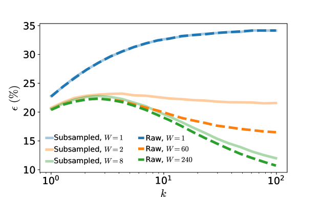
Figure 8: Subsampling effects. We compare the error of AR models trained on original raw dataset and the subsampled one with a subsampling factor of $s=30$. The key qualitative features of the error curves as function of the non-Markovianity $k$ are not affected by subsampling.

B.3 The thresholding algorithm

As a baseline benchmark, we consider a simple thresholding algorithm, where $\hat{c}_{t}=\mathrm{sgn}(x_{t})$. Put simply, this algorithm infers the potential’s location by only considering the position of the particle at a single point $x_{t}$ and choose the closest configuration of potential $c_{t}$ to that position. In fig. 9 we compare the performance of the AR(1) model with the thresholding algorithm and observe that AR(1) matches the performance of the the thresholding algorithm.

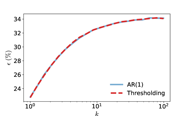
Figure 9: Comparing the AR(1) and the thresholding algorithm. Both the AR(1) model and the thresholding algorithm only have access to the position of the particle at a single point. As a consistency check we compare the performance of the two and observe that they match.

B.4 Selecting the best GRU(1) model

To find the best performing GRU(1) we train model for all $k$ values shown in fig. 5 we train five different instance of the network initialized randomly using as suggested in Ref. [65]. We choose the best performing model over 10000 samples for each $k$, and report the accuracy on a new set of 10000 samples. As shown in fig. 10 the test and cross validation accuracy are in excellent agreement.

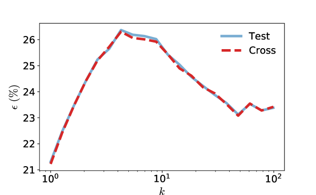
Figure 10: Validating the GRU(1) model. The accuracy of the best performing GRU(1) models over the cross validation and test sets match.

References

- [1] Jacob Devlin, Ming-Wei Chang, Kenton Lee and Kristina Toutanova “BERT: Pre-training of Deep Bidirectional Transformers for Language Understanding”, 2019 arXiv:1810.04805
- [2] Jeremy Howard and Sebastian Ruder, 2018 arXiv:1801.06146
- [3] Alec Radford and Karthik Narasimhan “Improving language understanding by generative pre-training”, 2018
- [4] Tom Brown and Benjamin Mann “Language Models are Few-Shot Learners” In Advances in Neural Information Processing Systems 33 Curran Associates, Inc., 2020, pp. 1877–1901 URL: https://proceedings.neurips.cc/paper_files/paper/2020/file/1457c0d6bfcb4967418bfb8ac142f64a-Paper.pdf
- [5] OpenAI “GPT-4 Technical Report” In arXiv preprint arXiv:2303.08774v2, 2023
- [6] Holger Kantz and Thomas Schreiber “Nonlinear time series analysis” Cambridge university press, 2004
- [7] George EP Box, Gwilym M Jenkins, Gregory C Reinsel and Greta M Ljung “Time series analysis: forecasting and control” John Wiley & Sons, 2015
- [8] Elizabeth Gardner and Bernard Derrida “Three unfinished works on the optimal storage capacity of networks” In Journal of Physics A: Mathematical and General 22.12 IOP Publishing, 1989, pp. 1983
- [9] Hyunjune Sebastian Seung, Haim Sompolinsky and Naftali Tishby “Statistical mechanics of learning from examples” In Physical review A 45.8 APS, 1992, pp. 6056
- [10] Andreas Engel and Christian Van den Broeck “Statistical mechanics of learning” Cambridge University Press, 2001
- [11] Marc Mezard and Andrea Montanari “Information, physics, and computation” Oxford University Press, 2009
- [12] Giuseppe Carleo et al. “Machine learning and the physical sciences” In Reviews of Modern Physics 91.4 APS, 2019, pp. 045002
- [13] A. Krizhevsky, I. Sutskever and G.E. Hinton “Imagenet classification with deep convolutional neural networks” In Advances in neural information processing systems, 2012, pp. 1097–1105
- [14] K. Simonyan and A. Zisserman “Very Deep Convolutional Networks for Large-Scale Image Recognition” In International Conference on Learning Representations, 2015
- [15] Kaiming He, Xiangyu Zhang, Shaoqing Ren and Jian Sun “Deep residual learning for image recognition” In Proceedings of the IEEE conference on computer vision and pattern recognition, 2016, pp. 770–778
- [16] Alexey Dosovitskiy et al. “An Image is Worth 16x16 Words: Transformers for Image Recognition at Scale” In International Conference on Learning Representations, 2021 URL: https://openreview.net/forum?id=YicbFdNTTy
- [17] Phil Pope et al. “The Intrinsic Dimension of Images and Its Impact on Learning” In International Conference on Learning Representations, 2021 URL: https://openreview.net/forum?id=XJk19XzGq2J
- [18] SueYeon Chung, Daniel D. Lee and Haim Sompolinsky “Classification and Geometry of General Perceptual Manifolds” In Phys. Rev. X 8 American Physical Society, 2018, pp. 031003 DOI: 10.1103/PhysRevX.8.031003
- [19] S. Goldt, M. Mézard, F. Krzakala and L. Zdeborová “Modeling the influence of data structure on learning in neural networks: The hidden manifold model” In Phys. Rev. X 10.4, 2020, pp. 041044
- [20] Sebastian Goldt et al. “The Gaussian equivalence of generative models for learning with shallow neural networks” In Proceedings of the 2nd Mathematical and Scientific Machine Learning Conference 145, Proceedings of Machine Learning Research PMLR, 2022, pp. 426–471 URL: https://proceedings.mlr.press/v145/goldt22a.html
- [21] Behrooz Ghorbani, Song Mei, Theodor Misiakiewicz and Andrea Montanari “When do neural networks outperform kernel methods?” In Advances in Neural Information Processing Systems 33, 2020
- [22] Dominic Richards, Jaouad Mourtada and Lorenzo Rosasco “Asymptotics of Ridge(less) Regression under General Source Condition” In Proceedings of The 24th International Conference on Artificial Intelligence and Statistics 130, Proceedings of Machine Learning Research PMLR, 2021, pp. 3889–3897 URL: https://proceedings.mlr.press/v130/richards21b.html
- [23] Lenaic Chizat and Francis Bach “Implicit bias of gradient descent for wide two-layer neural networks trained with the logistic loss” In Conference on Learning Theory, 2020, pp. 1305–1338 PMLR
- [24] Maria Refinetti, Sebastian Goldt, Florent Krzakala and Lenka Zdeborová “Classifying high-dimensional Gaussian mixtures: Where kernel methods fail and neural networks succeed” In Proceedings of the 38th International Conference on Machine Learning 139, Proceedings of Machine Learning Research PMLR, 2021, pp. 8936–8947 URL: https://proceedings.mlr.press/v139/refinetti21b.html
- [25] Bruno Loureiro et al. “Learning Gaussian Mixtures with Generalized Linear Models: Precise Asymptotics in High-dimensions” In Advances in Neural Information Processing Systems 34, 2021
- [26] Stefano Spigler, Mario Geiger and Matthieu Wyart “Asymptotic learning curves of kernel methods: empirical data versus teacher–student paradigm” In Journal of Statistical Mechanics: Theory and Experiment 2020.12 IOP Publishing, 2020, pp. 124001
- [27] Stéphane d’Ascoli, Marylou Gabrié, Levent Sagun and Giulio Biroli “On the interplay between data structure and loss function in classification problems” In Advances in Neural Information Processing Systems 34 Curran Associates, Inc., 2021, pp. 8506–8517 URL: https://proceedings.neurips.cc/paper/2021/file/47a5feca4ce02883a5643e295c7ce6cd-Paper.pdf
- [28] Marcus K. Benna and Stefano Fusi “Place cells may simply be memory cells: Memory compression leads to spatial tuning and history dependence” In Proceedings of the National Academy of Sciences 118.51, 2021, pp. e2018422118 DOI: 10.1073/pnas.2018422118
- [29] Federica Gerace et al. “Probing transfer learning with a model of synthetic correlated datasets” In Machine Learning: Science and Technology 3.1 IOP Publishing, 2022, pp. 015030 DOI: 10.1088/2632-2153/ac4f3f
- [30] Behrooz Ghorbani, Song Mei, Theodor Misiakiewicz and Andrea Montanari “Limitations of Lazy Training of Two-layers Neural Network” In Advances in Neural Information Processing Systems 32, 2019, pp. 9111–9121
- [31] Gennaro Tucci et al. “Modeling active non-Markovian oscillations” In Physical Review Letters 129.3 APS, 2022, pp. 030603
- [32] Patrick Pietzonka, Felix Ritort and Udo Seifert “Finite-time generalization of the thermodynamic uncertainty relation” In Physical Review E 96.1 APS, 2017, pp. 012101
- [33] I Di Terlizzi et al. “Variance sum rule for entropy production” In arXiv preprint arXiv:2302.08565, 2023
- [34] N.. Van Kampen “Stochastic processes in physics and chemistry” Elsevier, 1992
- [35] Ignacio A Martinez and Dmitri Petrov “Force mapping of an optical trap using an acousto-optical deflector in a time-sharing regime” In Applied optics 51.22 Optical Society of America, 2012, pp. 5522–5526
- [36] Ignacio A Martínez, Edgar Roldán, Juan MR Parrondo and Dmitri Petrov “Effective heating to several thousand kelvins of an optically trapped sphere in a liquid” In Physical Review E 87.3 APS, 2013, pp. 032159
- [37] Y. LeCun et al. “Backpropagation Applied to Handwritten Zip Code Recognition” In Neural Computation 1.4, 1989, pp. 541–551 DOI: 10.1162/neco.1989.1.4.541
- [38] Ian Goodfellow, Yoshua Bengio and Aaron Courville “Deep learning” MIT press, 2016
- [39] Kunihiko Fukushima “Visual Feature Extraction by a Multilayered Network of Analog Threshold Elements” In IEEE Transactions on Systems Science and Cybernetics 5.4, 1969, pp. 322–333 DOI: 10.1109/TSSC.1969.300225
- [40] Kyunghyun Cho, Bart Merriënboer, Dzmitry Bahdanau and Yoshua Bengio “On the Properties of Neural Machine Translation: Encoder–Decoder Approaches” In Proceedings of SSST-8, Eighth Workshop on Syntax, Semantics and Structure in Statistical Translation, 2014, pp. 103–111
- [41] Diederik P Kingma and Jimmy Ba “Adam: A method for stochastic optimization” In arXiv preprint arXiv:1412.6980, 2014
- [42] Peter E Kloeden and Eckhard Platen “Stochastic differential equations” In Numerical Solution of Stochastic Differential Equations Springer, 1992, pp. 103–160
- [43] Alessio Lapolla and Aljaz Godec “Toolbox for quantifying memory in dynamics along reaction coordinates” In Physical Review Research 3.2 APS, 2021, pp. L022018
- [44] Alessio Lapolla and Aljaz Godec “Manifestations of projection-induced memory: General theory and the tilted single file” In Frontiers in Physics 7 Frontiers, 2019, pp. 182
- [45] Elsi-Mari Laine, Jyrki Piilo and Heinz-Peter Breuer “Measure for the non-Markovianity of quantum processes” In Physical Review A 81.6 APS, 2010, pp. 062115
- [46] Michael JW Hall, James D Cresser, Li Li and Erika Andersson “Canonical form of master equations and characterization of non-Markovianity” In Physical Review A 89.4 APS, 2014, pp. 042120
- [47] Ángel Rivas, Susana F Huelga and Martin B Plenio “Entanglement and non-Markovianity of quantum evolutions” In Physical review letters 105.5 APS, 2010, pp. 050403
- [48] Zhiqiang Huang and Xiao-Kan Guo “Quantifying non-Markovianity via conditional mutual information” In Physical Review A 104.3 APS, 2021, pp. 032212
- [49] Philipp Strasberg and Massimiliano Esposito “Response functions as quantifiers of non-Markovianity” In Physical review letters 121.4 APS, 2018, pp. 040601
- [50] Aaron M Ellison “Effect of seed dimorphism on the density-dependent dynamics of experimental populations of Atriplex triangularis (Chenopodiaceae)” In American Journal of Botany 74.8 Wiley Online Library, 1987, pp. 1280–1288
- [51] Sepp Hochreiter and Jürgen Schmidhuber “Long short-term memory” In Neural computation 9.8 MIT Press, 1997, pp. 1735–1780
- [52] Haim Sompolinsky, Andrea Crisanti and Hans-Jurgen Sommers “Chaos in random neural networks” In Physical review letters 61.3 APS, 1988, pp. 259
- [53] David Sussillo and Larry F Abbott “Generating coherent patterns of activity from chaotic neural networks” In Neuron 63.4 Elsevier, 2009, pp. 544–557
- [54] Francesca Mastrogiuseppe and Srdjan Ostojic “Linking connectivity, dynamics, and computations in low-rank recurrent neural networks” In Neuron 99.3 Elsevier, 2018, pp. 609–623
- [55] Friedrich Schuessler et al. “The interplay between randomness and structure during learning in RNNs” In Advances in neural information processing systems 33, 2020, pp. 13352–13362
- [56] Gabriel B Mindlin “Nonlinear dynamics in the study of birdsong” In Chaos 27.9 AIP Publishing LLC, 2017, pp. 092101
- [57] Guido Vettoretti and W Richard Peltier “Fast physics and slow physics in the nonlinear Dansgaard–Oeschger relaxation oscillation” In J. Clim. 31.9, 2018, pp. 3423
- [58] Massimo Cavallaro and Rosemary J Harris “Effective bandwidth of non-Markovian packet traffic” In Journal of Statistical Mechanics: Theory and Experiment 2019.8 IOP Publishing, 2019, pp. 083404
- [59] Édgar Roldán et al. “Quantifying entropy production in active fluctuations of the hair-cell bundle from time irreversibility and uncertainty relations” In New Journal of Physics 23.8 IOP Publishing, 2021, pp. 083013
- [60] Roman Belousov, Florian Berger and AJ Hudspeth “Volterra-series approach to stochastic nonlinear dynamics: Linear response of the Van der Pol oscillator driven by white noise” In Phys. Rev. E 102.3 APS, 2020, pp. 032209
- [61] David B Brückner et al. “Stochastic nonlinear dynamics of confined cell migration in two-state systems” In Nat. Phys. 15.6 Nature Publishing Group, 2019, pp. 595
- [62] Dominic J. Skinner and Jörn Dunkel “Estimating Entropy Production from Waiting Time Distributions” In Phys. Rev. Lett. 127 APS, 2021, pp. 198101
- [63] Sandeep Mavadia et al. “Prediction and real-time compensation of qubit decoherence via machine learning” In Nature communications 8.1 Nature Publishing Group, 2017, pp. 1–6
- [64] Swarnadeep Majumder, Leonardo Andreta de Castro and Kenneth R Brown “Real-time calibration with spectator qubits” In npj Quantum Information 6.1 Nature Publishing Group, 2020, pp. 1–9
- [65] Xavier Glorot and Yoshua Bengio “Understanding the difficulty of training deep feedforward neural networks” In Proceedings of the thirteenth international conference on artificial intelligence and statistics, 2010, pp. 249–256 JMLR WorkshopConference Proceedings