Time Evolution of a Decaying Quantum State:
Evaluation and Onset of Non-Exponential Decay

Abstract

The method developed by van Dijk, Nogami and Toyama [1, 2, 3, 4] for obtaining the time-evolved wave function of a decaying quantum system is generalized to potentials and initial wave functions of non-compact support. The long time asymptotic behavior is extracted and employed to predict the timescale for the onset of non-exponential decay. The method is illustrated with a Gaussian initial wave function leaking through Eckart’s potential barrier on the halfline.

I Introduction

Quantum tunneling, the phenomenon of a particle traversing a potential barrier higher than its kinetic energy, has received a great deal of attention since the early works of Gamow [5]. Despite the time and effort spent on this issue (see [6, 7, 8, 9] for important contributions to the discussion and reviews and [10] for a recent experiment), there still remain open questions about tunneling. One reason for this is that while tunneling is fundamentally a process in time, much of the analysis has been restricted to static aspects of the relevant setups. While important properties of tunneling systems such as exponential decay rates describing a decaying system for intermediate times can be found in such an analysis, a more thorough understanding seems desirable.

For this reason studying the time dependent wave function describing the tunneling particle is essential to complete the picture. For the setup of a decaying quantum state a great deal of progress in this direction has been achieved by van Dijk, Nogami and Toyama [1, 2, 3, 4]. For a precursor to the technique see [11]. They found a representation of the time dependent wave function well suited for studying early, intermediate and late times. This makes it well suited for analytic as well as numerical endeavors. The method was only applied to compactly supported potentials and initial wave functions. The compact support of the initial wave function played an important role, as will be explained in the next section. In this article I extend this method and apply it to a Gaussian initial wave packet leaking out of Eckart’s potential barrier; neither of which has a compact support. The necessary modification of the technique is introduced first.

Following a reminder of the tricks employed and the generalization of the present work I analyze the late-time asymptotics. While the power-law for the decay of the wave function

$$|\psi(r,t)|\overset{t\rightarrow\infty}{\rightarrow}\frac{|\psi_{\infty}(r)|}{t^{3/2}},$$ (1)

in the generic case is well-known, I derive a simple and fairly general expression for the constant involved cf. [12]. Furthermore, an estimate of the time $t_{\text{alg}}$ after which the transition from exponential to algebraic decay takes place is given in (29). This result should be compared to the one for the survival amplitude by [13]. For a complicated barrier it may not be feasible to apply the full technique while the expressions for $|\psi_{\infty}(r)|$ and $t_{\text{alg}}$ can be evaluated more easily and may therefore be of greater importance when comparing with experiments.

II Recap and Extension

II.1 Main Argument

We consider the Schrödinger equation (setting $\hbar=2m=1$)

$$i\partial_{t}\psi=-\partial_{r}^{2}\psi+V\psi,$$ (2)

for the scalar wave function $\psi$ subject to the potential $V$ and boundary condition $\psi(0,t)=0$ for all $t$, chosen such that there are no bound states . This theoretical setup may describe the radial part of a system describing alpha-decay with zero angular momentum [15] or it may describe the motion of an ion along the axis of a quantum optical trap inducing a back wall [16, 17] and an extra trapping potential $V$. We will make use of the Jost solutions $f(k,r)$ of (2) which are the generalized eigenfunctions of the Hamiltonian of (2) of energy $k^{2}$ that satisfy

$$\lim_{r\rightarrow\infty}e^{-ikr}f(k,r)=1.$$ (3)

Jost solutions exist for potentials $V$ such that $\int_{0}^{\infty}dr\,r|V(r)|<\infty$. For fixed real $r$ the Jost solution $f(k,r)$ is analytic on $\{\operatorname{Im}(k)\geq 0\wedge k\neq 0\}\subset\mathbb{C}$ and fulfills $\overline{f(k,r)}=f(-\overline{k},r)$ [18, Thm XI.57]. Furthermore, I assume that 0 is not an eigenvalue or resonance of the Hamiltonian involved, which is typically true.

The generalized eigenfunction $u(k,r)$ of the same energy satisfying the proper boundary condition at the origin and the additional normalization

$$u(k,0)=0,\quad u^{\prime}(k,0)=1,$$ (4)

where the prime denotes a derivative with respect to the second argument, is given by

$$u(k,r)=\big{(}f(k,0)f(-k,r)-f(-k,0)f(k,r)\big{)}\frac{1}{2ik}.$$ (5)

Furthermore, $u(k,r)$ is real for real $r$ and $k$ and even in $k$ and for $r$ fixed $u(k,r)$ is an entire function of $k$ [18, Thm XI.56]. The solutions $u$ form a complete set and are normalized to [1]

$$\int_{0}^{\infty}\overline{u(k,r)}u(k^{\prime},r)dr=\frac{\pi}{2k^{2}}|f(k,0)|^{2}\delta(k-k^{\prime}),$$ (6)

for $k,k^{\prime}>0$. So we may expand any solution $\psi(x,t)$ of equation (2):

$$\psi(r,t)=\frac{2}{\pi}\int_{0}^{\infty}\frac{k^{2}}{f(k,0)f(-k,0)}C(k)e^{-ik^{2}t}u(k,r)dk,$$ (7)

with

$$C(k)=\int_{0}^{\infty}u(k,r)\psi(r,0)dr,$$ (8)

where I eliminated complex conjugates by the above mentioned properties of $u$ and $f$. Because of the symmetry properties of the integrand I split $u$ up as in equation (5) to obtain

$$\psi(r,t)=\int_{-\infty}^{\infty}e^{-ik^{2}t+ikr}\frac{C(k)}{i\pi}\frac{k\,e^{-ikr}f(-k,r)}{f(-k,0)}dk,$$ (9)

where I added an additional plane wave so that the last factor approaches a finite limit for $r\rightarrow\infty$. Next I introduce an auxiliary factor $h(k)$

$$\psi(r,t)=\frac{1}{i\pi}\int_{-\infty}^{\infty}e^{-ik^{2}t+ikr}h(k)\overbrace{\frac{k\,C(k)e^{-ikr}f(-k,r)}{h(k)f(-k,0)}}^{=:g(k,r)}dk,$$ (10)

to achieve the following properties:

• The fraction $g(k,r)$ is still meromorphic in $k$.

• The expansion of $g(k,r)$ by the Mittag-Leffler [19] theorem is of the form

  $$g(k,r)=\sum_{n}\frac{a_{n}(r)}{k-k_{n}},$$ (11)

  where $a_{n}$ are the residues of $g$ at it’s poles $k_{n}$. A sufficient criterion for (11) is that $g(k,r)$ falls off at infinity in the complex $k-$plane (excluding small circles around the poles) and the sum in (11) converges uniformly on compact sets.

• The integral that remains after exchange of integral and sum which is of the form

  $$\frac{1}{i\pi}\int_{-\infty}^{\infty}\frac{e^{-ik^{2}t+ikr}h(k)}{k-k_{n}},$$ (12)

  may be evaluated in closed form.

In [1, 2, 3, 4], the initial wave functions $\psi(r,0)$ under consideration vanishes for any $r>R$ for some $R>0$, this results in growth of the fractions of (9) like $e^{-\mathrm{Im}(k)R}$ in negative imaginary direction. The choice $h=e^{ikR}$ exactly cancelles this growth so that Mittag-Leffler can be applied.

The central innovation of the current paper is a different choice of $h$ so as to allow for more generality:

$$h_{\alpha}(k)=e^{i\alpha k^{2}}+e^{-i\alpha k^{2}}+e^{-\alpha k^{2}},$$ (13)

where $\alpha>0$ is a free parameter.

To give an idea of which initial wave functions can be treated with this method a quick estimate of the growth of $C(k)$ in imaginary direction may be helpful. From general scattering theory we know that the eigenfunctions $u$ generically grow exponentially in the complex plane see [20, equation (12.8)], [21, equations (6.4.13) and (6.4.17)]

$$|u(k,r)|\leq\frac{c_{1}}{|k|}e^{|\operatorname{Im}(k)|r}.$$ (14)

If we assume that $\psi(r,0)=\mathcal{O}\left(e^{-c_{2}r^{c_{3}}}\right)$ for some $c_{2}>0,c_{3}>1$ for $r\rightarrow\infty$ big enough a stationary phase argument yields

$$|C(k)|\leq c_{4}e^{(c_{2}c_{3})^{\frac{-1}{c_{3}-1}}(\left|\mathrm{Im}(k)\right|)^{\frac{c_{3}}{c_{3}-1}}(1-1/c_{3})}.$$ (15)

If this growth can be controlled by a Gaussian the choice (13) will work for some $\alpha>0$. Hence for any initial wave function with $c_{3}\geq 2$ the method will succeed.

The choice (13) results in the following expression for the wave function

$$\psi(r,t)=\sum_{n}a_{n}(r)\sum_{\gamma\in\{\alpha,\pm i\alpha\}}M(k_{n},r,\gamma +it),$$ (16)

where $M$ is given by

$$M(k,r,\beta)=\int_{-\infty}^{\infty}\frac{dp}{i\pi}\frac{e^{-\beta p^{2}+irp}}{p-k}$$ (17)

$$=e^{ikr-\beta k^{2}}\bigg{[}\text{sgn}(\text{Im}(k))+\operatorname{erf}\big{(}(r+2ik\beta)/(2\sqrt{\beta})\big{)}\bigg{]}$$

and is closely related to the Moshinsky function [22]. In order to apply the method one has to include all the poles of $g$, including the zeros of $h_{\alpha}$, which are located close to the three sets

$$\left\{\pm e^{-\frac{3\pi i}{8}}\sqrt{\pi(2n-1)/(\sqrt{2}\alpha)}\,\bigg{|}n\in\mathbb{N}\right\},$$ (18)

$$\left\{\pm e^{\frac{3\pi i}{8}}\sqrt{\pi(2n-1)/(\sqrt{2}\alpha)}\,\bigg{|}n\in\mathbb{N}\right\},$$ (19)

$$\left\{\pm\sqrt{\pi(2n-1)/(2\alpha)}\,\bigg{|}n\in\mathbb{N}\right\}.$$ (20)

II.2 Late Time Asymptotics

Besides the apparent use of the representation (16) to calculate $\psi(r,t)$ numerically with small error for early as well as for late times it is also useful for theoretical considerations which is illustrated by this chapter. I will discuss the late time asymptotics of a decaying quantum system recovering the well known result

$$\psi(r,t)\xrightarrow{t\rightarrow\infty}\frac{\psi_{\infty}(r)}{t^{3/2}},$$ (21)

valid vor generic wave functions. Please note, that for special initial wave functions a different power law may apply [23]. The asymptotic behavior (21) was e.g. also obtained by [3, 8, 12] for rigorous bounds see [21, 24, 25]. The amplitude $\psi_{\infty}(r)$ will be obtained for any system to which the method of the last section is applicable and to arbitrary accuracy in the expansion (16). This expression is simpler than the one of [12]. For $t$ large relative to $r$ and $\alpha$, I employ the asymptotic expression for $\operatorname{erf}$ [26, page 109-112]

$$\operatorname{erf}(\pm z) =\pm 1-\frac{e^{-z^{2}}}{\sqrt{\pi}}\sum_{k=0}^{M}\frac{(-1)^{k}\left(\frac{1}{2}\right)_{k}}{(\pm z)^{2k+1}}+\mathcal{O}(e^{-z^{2}}z^{-2M-3}),$$ (22)

valid for $|\operatorname{ph}(\pm z)|<\frac{3}{4}\pi$ where the phase of $k_{n}$ decides which of the two expansions is to be used and $(c)_{k}$ is the Pochhammer-symbol. Taking $\gamma\in\{\alpha,\pm i\alpha\}$ and using (22) I get

$$\!M(k_{n},r,\gamma+it)\approx e^{ik_{n}r-(it+\gamma)k_{n}^{2}}(\operatorname{sgn}(\operatorname{Im}(k_{n}))+\nu)$$ (23)

$$-\frac{\sqrt{it+\gamma}e^{\frac{-r^{2}}{4(it+\gamma)}}}{\sqrt{\pi}(\frac{r}{2}+ik_{n}(it+\gamma))}\left(1-\frac{(it+\gamma)/2}{\big{(}\frac{r}{2}+ik_{n}(it+\gamma)\big{)}^{2}}\right),$$

with $\nu=-1$ for $k_{n}=|k_{n}|e^{i\varphi}$ and $-\frac{1}{4}\pi\leq\varphi\leq\frac{3}{4}\pi$ and $\nu=1$ otherwise. I omitted errors of order $\mathcal{O}(t^{-5/2})$. There are several remarks in order:

• Except for the case $k_{n}\in\mathbb{R}$ the first summand in (23) is either identically zero or decays exponentially in time for their respective region of $\varphi$ and may therefore be absorbed into the error.

• For a $k_{n}\in\mathbb{R}$, the first term is oscillatory. However, in this case $h_{\alpha}(k_{n})=0$ as the Jost solution $f(-k,0)$ has no zeros and $C(k)$ no poles on the real line. Hence the first term of (23) vanishes in the sum over $\gamma\in\{\alpha,\pm i\alpha\}$.

• The complicated fractions involving $k_{n},r$ and $t$ may be represented by a series in inverse powers of $t$, which will also be a series in inverse powers of $k_{n}$. We may then exploit the absence of a constant term in (11) to obtain

  $$0 =\sum_{n}\frac{a_{n}(r)}{k_{n}},$$ (24)

  $$\frac{C(0)}{3}\frac{f(0,r)}{f(0,0)} =-\sum_{n}\frac{a_{n}(r)}{k_{n}^{2}}$$ (25)

  $$\frac{C(0)}{3}\partial_{k}\left.\frac{e^{-ikr}f(-k,r)}{f(-k,0)}\right|_{k=0} =-\sum_{n}\frac{a_{n}(r)}{k_{n}^{3}}$$ (26)

  by inserting $k=0$ into (11) and its derivatives. This yields a simpler expression for the asymptotically late wave function.

As a next step I employ the binomial series to express the fractions in (23) and sum over the three possibilities of $\gamma\in\{\alpha,\pm i\alpha\}$ and over all poles $k_{n}$, this results in

$$\psi_{\infty}(r)=-\frac{C(0)}{2\sqrt{i\pi}}\partial_{k}\left.\frac{f(-k,r)}{f(-k,0)}\right|_{k=0}.$$ (27)

Corrections to (21) are of order $\mathcal{O}\left(t^{-5/2}\right)$. If $C(0)=0$ the decay of $\psi(r,t)$ for large $t$ will be faster, as observed in [23]. Higher orders can be worked out analogously to extract an asymptotic series for $\psi(r,t)$ in $1/\sqrt{t}$, which implies a series of the same kind for

$$P(t)=\int_{0}^{\rho}|\psi(r,t)|^{2}dr,$$ (28)

the probability of finding the particle inside the trapping region of length $\rho$. The use of the binomial series is only justified for late times, where what “late” means depends on $r$. This onset of the algebraic decay can be estimated by equating the exponential term with slowest decay of (23) with the term (27), yielding:

$$t_{\text{alg}}=\frac{-3/2}{|\operatorname{Im}k_{0}^{2}|}W_{-1}\!\!\left(\frac{-|\operatorname{Im}k_{0}^{2}|}{3/2^{1/3}}\left|\frac{\psi_{\infty}(r)\partial_{k_{0}}f(-k_{0},0)}{k_{0}C(k_{0})f(-k_{0},r)}\right|^{2/3}\right),$$ (29)

where $W_{-1}$ is the $-1$-branch of the Lambert W function and $k_{0}$ is the wave vector belonging to the slowest exponential decay, i.e. the zero of $f(-k,0)$ in the fourth quadrant of the complex plane closest to the origin.

Besides (28) the survival probability

$$S(t)=\left|\int_{0}^{\infty}\psi^{*}(r,0)\psi(r,t)dr\right|^{2},$$ (30)

is often used to study decaying quantum states. The long time limit of $S(t)$ can be found pluggin in (7) and (6):

$$S(t)=\left|\frac{1}{\pi}\int_{-\infty}^{\infty}\frac{k^{2}C^{\prime}(k)C(k)}{f(k,0)f(-k,0)h_{\alpha}(k)}e^{-ik^{2}t}h_{\alpha}(k)dk\right|^{2},$$ (31)

with

$$C^{\prime}(k)=\int_{0}^{\infty}u(k)\psi^{*}(r)dr.$$ (32)

So that Mittag-Leffler can be applied again to obtain

$$S(t)=\left|\sum_{n}b_{n}\sum_{\gamma\in\{\alpha,\pm i\alpha\}}M(k_{n},0,\gamma+it)\right|^{2}.$$ (33)

Using the same expansion and manipulations as for the the long time limit of $\psi$ then yields:

$$S(t)\xrightarrow{t\rightarrow\infty}\frac{1}{t^{3}}~{}\frac{|C(0)|^{4}}{4\pi(f(0,0))^{4}},$$ (34)

showing that $S$ has the same power law as $P$ and also decays faster if $C(0)=0$. Evaluating expansions (16) and (33) without closed form expressions for $f$ is difficult, this is not the case for equations (27) and (34). They may be evaluated numerically for any potential $V$ such that the growth conditions on the Jost solution $f$ and the integrals over the initial wave function $C$ are fulfilled. Hence these considerations of late times may be of some use to test non-relativistic models of alpha-decay when compared to experiment.

III Application to Eckart’s potential

Eckart’s potential

$$V(r)=\frac{Ae^{r-\rho}}{\left(1+e^{r-\rho}\right)^{2}},$$ (35)

where $\rho\in\mathbb{R}$ and $A\in\mathbb{R}$ are free parameters together with the initial wave function

$$\psi_{0}(r)=\frac{2^{5/2}}{\rho^{3/2}\sqrt[4]{\pi}}re^{-2\left(\frac{r}{\rho}\right)^{2}}$$ (36)

provides a nice example for which an exponential choice of $h$ would not suffice. This potential has been used to study tunneling [28] from the perspective of theoretical physics as well as from the perspective of chemistry [29]. The associated Jost solution is given by [8, 30]

$$f(k,r)=e^{-ikr}{}_{2}F_{1}\Big{(}\frac{1}{2}-i\delta,\frac{1}{2}+i\delta;1+2ik;\frac{1}{1+e^{r-\rho}}\Big{)},$$ (37)

with $\delta=\sqrt{A-1/4}$, where ${}_{2}F_{1}$ is the Gauss hypergeometric function.

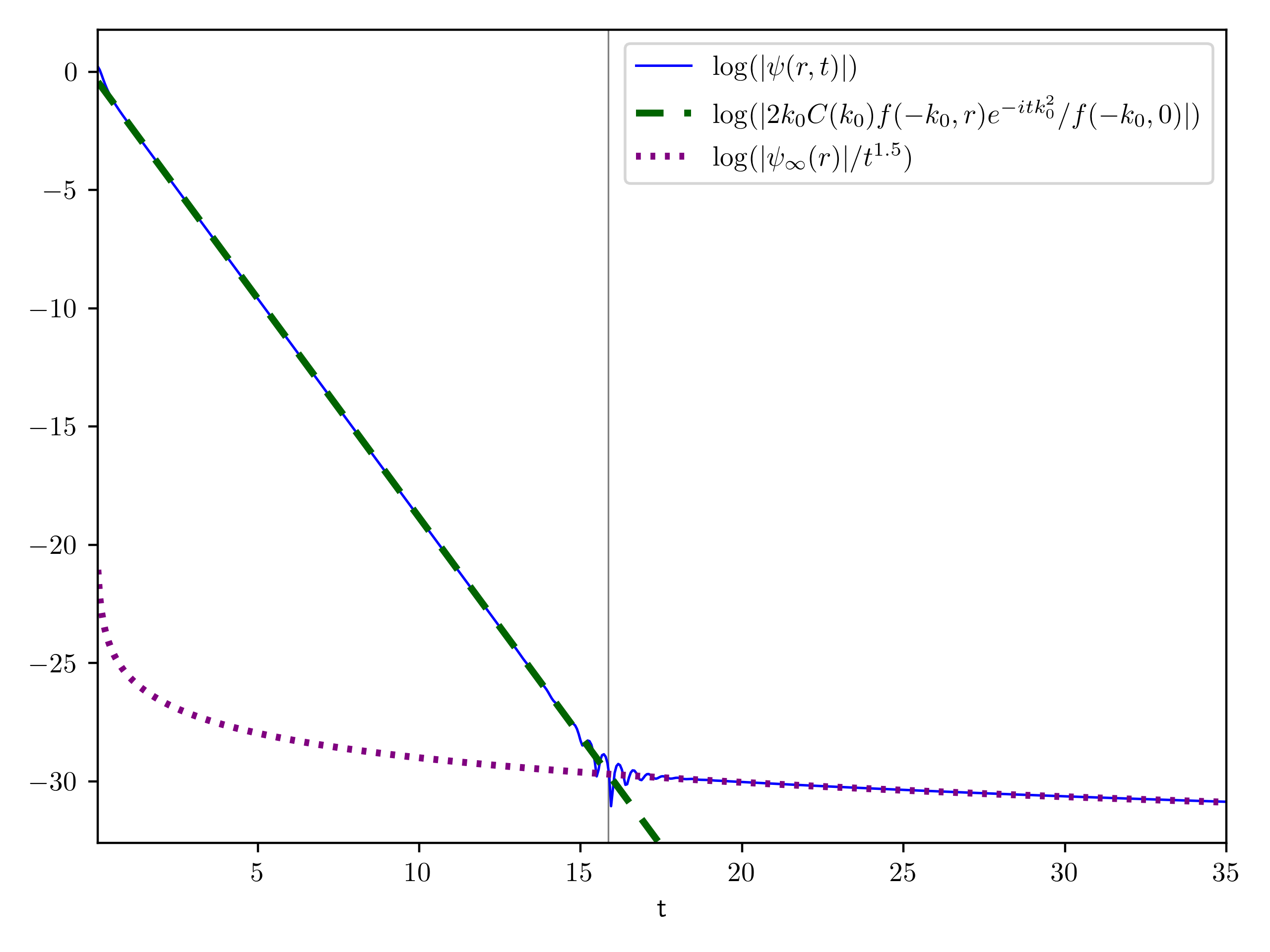
Figure 1: Numerical logarithmic comparison of $|\psi(r,t)|$, $|\psi_{\infty}(r)|/t^{1.5}$ and the slowest exponential decay corresponding to the zero $k_{0}$ of $f(-k,0)$ closest to the origin in the fourth quadrant. The thin vertical line marks $t_{\text{alg}}$. The parameters are $A=49.25,\rho=1,r=0.5$ and $\alpha=1.25$. To compute $\psi(r,t)$ all summands of (16) corresponding to poles $|k_{n}|<100$, which results in approximately 18000 summands. The code that produced this figure can be found here: %****␣script.tex␣Line␣450␣****https://gitlab.com/therunomask/tunneling, it uses mpmath [31].

In this setup the Mittag-Leffler theorem implies (11)

$$g(k,r)=\frac{kC(k)e^{-ikr}f(-k,r)}{h_{\alpha}(k)f(-k,0)}=\sum_{n}\frac{a_{n}(r)}{k-k_{n}}.$$ (38)

The main reason why my choice of $h_{\alpha}$ works while an exponential one does not is as follows:

The generalized Fourier transform of of the initial wave function, $C(k)$, satisfies the bound

$$|C(k)|\leq\frac{\sqrt{2}\sqrt{\rho}c_{1}}{|k|\sqrt[4]{\pi}}+4c_{1}\sqrt[4]{\pi}\rho^{3/2}e^{\rho^{2}|\operatorname{Im}(k)|^{2}},$$ (39)

which can be derived using (14). The $\leq$ becomes $\approx$ for $|k|$ large enough and $k\not\in\mathbb{R}$. This can be compensated for by my choice of $h_{\alpha}$ for $\alpha$ big enough, while clearly an exponential $h$ does not suffice.

A detailed estimate on the real line shows

$$C(k)=\mathcal{O}(k^{-6}),\quad k\rightarrow\infty$$ (40)

implying that the sum (16) converges. In order to evaluate (16), the pole structure of $g$ should be studied. Here, in addition to the artificial poles close to (18), (19) and (20) there are poles due to the Jost solution $f$. It has poles at $k=in/2$ for $n\in\mathbb{N}$, however the poles cancel in the expression for $g$, as they appear in the numerator as well as the denominator. The function $f(-k,0)$ has zeros for complex $k$, symmetric about the imaginary axis. I conjecture the right arm of which approaches

$$k_{n}=\frac{n-\frac{1}{4}+\frac{i}{2\pi}\ln\Big{(}e^{\pi\delta}+e^{-\pi\delta}\Big{)}}{i+\frac{\rho}{\pi}}$$ (41)

for large $n$. This conjecture is supported by numerical evidence, but I do not have a proof yet.

In figure 1 all of the above is used to check numerically how accurately $t_{\text{alg}}$ reflects the transition from exponential to algebraic decay for the arbitrary choice $r=1/2$. The behavior seen in figure 1 is consistent with the analysis in [3].

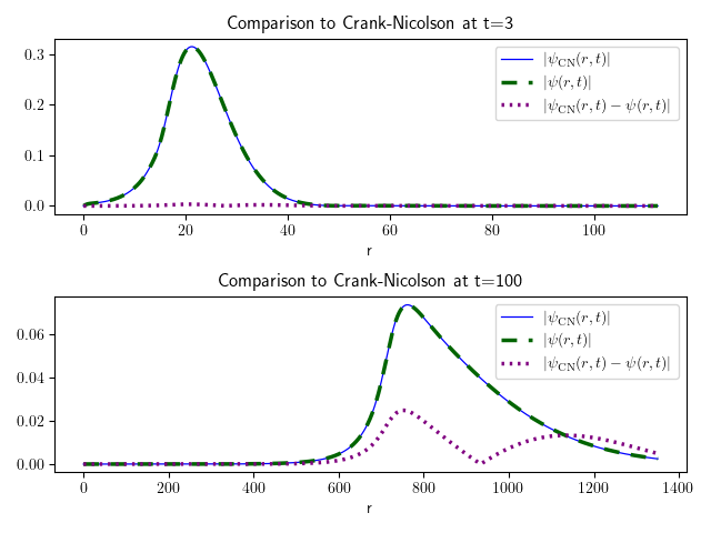
Figure 2: Comparison of evaluation of (16) with $A=49.25$, $\rho=1$ and $\alpha=1.25$ with the Crank-Nicolson (CN) method at $t=3$ and $t=100$. All poles with $|k_{n}|\leq 120$ are taken into account for (16). The discretization parameters for CN are $\Delta r=0.01953125$ and $\Delta t=\Delta r^{2}/4$, the length of the simulation box is $L=650$ for $t=3$ and $L=4480$ for $t=100$. The CN method is implemented in Julia [32], the code that produces this figure can also be found here https://gitlab.com/therunomask/tunneling.

In figure 2 the evaluation of (16) is compared with the well established Crank-Nicolson method at an early ($t=3$) and moderately late ($t=100$) time. One can see clearly that the two methods agree reasonably well at early times and the absolute value of $|\psi|$ still agrees at $t=100$ while substantial phase difference has accumulated leading a large difference.

IV Conclusion

In the present paper I have generalized the method of van Dijk, Nogami, and Toyama [1, 2, 3, 4] to a large class of non-compactly supported potentials and initial wave functions which includes Gaussian initial states. This method was used to derive the asymptotic amplitude $|\psi_{\infty}(r)|$ as well as estimate the onset of algebraic decay $t_{\text{alg}}$ characteristic of large times. Finally, the method was applied to a Gaussian wave packet leaking through Eckart’s potential against a hard-backwall potential barrier.

V Disclaimer

This article reflects the author’s personal work and does not represent scientific standpoints of the author’s employer.

VI Acknowledgments

I wholeheartedly thank Christian Bild for meticulously checking my calculations as well as Siddhant Das for helpful discussions.

References

- van Dijk and Nogami [1999] W. van Dijk and Y. Nogami, Novel expression for the wave function of a decaying quantum system, Physical review letters 83, 2867 (1999).
- Nogami et al. [2000] Y. Nogami, F. Toyama, and W. van Dijk, Bohmian description of a decaying quantum system, Physics Letters A 270, 279 (2000).
- van Dijk and Nogami [2002] W. van Dijk and Y. Nogami, Analytical approach to the wave function of a decaying quantum system, Physical Review C 65, 024608 (2002).
- van Dijk and Toyama [2019] W. van Dijk and F. M. Toyama, Decay of a quasistable quantum system and quantum backflow, Physical Review A 100, 052101 (2019).
- Gamow [1928] G. Gamow, Zur quantentheorie des atomkernes, Zeitschrift für Physik 51, 204 (1928).
- Hartman [1962] T. E. Hartman, Tunneling of a wave packet, Journal of Applied Physics 33, 3427 (1962).
- Muga et al. [2007] G. Muga, R. S. Mayato, and I. Egusquiza, Time in quantum mechanics, Vol. 734 (Springer Science & Business Media, 2007).
- Razavy [2003] M. Razavy, Quantum theory of tunneling (World Scientific, 2003).
- Hauge and Støvneng [1989] E. Hauge and J. Støvneng, Tunneling times: a critical review, Reviews of Modern Physics 61, 917 (1989).
- Ramos et al. [2020] R. Ramos, D. Spierings, I. Racicot, and A. M. Steinberg, Measurement of the time spent by a tunnelling atom within the barrier region, Nature 583, 529 (2020).
- Garcıa-Calderón et al. [1996] G. Garcıa-Calderón, J. Mateos, and M. Moshinsky, Survival and nonescape probabilities for resonant and nonresonant decay, annals of physics 249, 430 (1996).
- Jensen and Kato [1979] A. Jensen and T. Kato, Spectral properties of schrödinger operators and time-decay of the wave functions, Duke mathematical journal 46, 583 (1979).
- Peres [1980] A. Peres, Nonexponential decay law, Annals of Physics 129, 33 (1980).
- Note [1] See [3] for how to modify the technique in the presence of bound states.
- Lovas et al. [1998] R. G. Lovas, R. Liotta, A. Insolia, K. Varga, and D. Delion, Microscopic theory of cluster radioactivity, Physics reports 294, 265 (1998).
- Das and Dürr [2019] S. Das and D. Dürr, Arrival time distributions of spin-1/2 particles, Scientific reports 9, 1 (2019).
- Das et al. [2019] S. Das, M. Nöth, and D. Dürr, Exotic bohmian arrival times of spin-1/2 particles: an analytical treatment, Physical Review A 99, 052124 (2019).
- Reed and Simon [1979] M. Reed and B. Simon, Scattering theory. methods of modern mathematical physics, vol. _3., Scattering theory. Methods of modern mathematical physics, Vol. _3., by Reed, M.; Simon, B.. New York, NY (USA): American Press, 15+ 463 p. (1979).
- Jeffreys et al. [1999] H. Jeffreys, B. Jeffreys, and B. Swirles, Methods of mathematical physics (Cambridge university press, 1999).
- Newton [1966] R. G. Newton, Scattering theory of waves and particles (Springer Science & Business Media, 1966).
- Vona [2014] N. Vona, On time in quantum mechanics, arXiv preprint arXiv:1403.2496 (2014).
- Moshinsky [1952] M. Moshinsky, Diffraction in time, Physical Review 88, 625 (1952).
- Miyamoto [2004] M. Miyamoto, Initial wave packets and the various power-law decreases of scattered wave packets at long times, Physical Review A 69, 042704 (2004).
- Journé et al. [1991] J.-L. Journé, A. Soffer, and C. D. Sogge, Decay estimates for schrödinger operators, Communications on Pure and Applied mathematics 44, 573 (1991).
- Schlag [2007] W. Schlag, Dispersive estimates for schrödinger operators: a survey, Mathematical aspects of nonlinear dispersive equations 163, 255 (2007).
- Olver [1997] F. Olver, Asymptotics and special functions (CRC Press, 1997).
- Note [2] Formulated in terms of lower incomplete gamma function.
- de la Cal et al. [2022] X. G. de la Cal, M. Pons, and D. Sokolovski, Speed-up and slow-down of a quantum particle, Scientific reports 12, 1 (2022).
- Migliore et al. [2014] A. Migliore, N. F. Polizzi, M. J. Therien, and D. N. Beratan, Biochemistry and theory of proton-coupled electron transfer, Chemical reviews 114, 3381 (2014).
- Eckart [1930] C. Eckart, The penetration of a potential barrier by electrons, Physical Review 35, 1303 (1930).
- Johansson et al. [2013] F. Johansson et al., mpmath: a Python library for arbitrary-precision floating-point arithmetic (version 0.18) (2013), http://mpmath.org/.
- Bezanson et al. [2017] J. Bezanson, A. Edelman, S. Karpinski, and V. B. Shah, Julia: A fresh approach to numerical computing, SIAM Review 59, 65 (2017), https://doi.org/10.1137/141000671 .