COFS: Controllable Furniture layout Synthesis

Abstract

Scalable generation of furniture layouts is essential for many applications in virtual reality, augmented reality, game development and synthetic data generation. Many existing methods tackle this problem as a sequence generation problem which imposes a specific ordering on the elements of the layout making such methods impractical for interactive editing or scene completion. Additionally, most methods focus on generating layouts unconditionally and offer minimal control over the generated layouts. We propose COFS, an architecture based on standard transformer architecture blocks from language modeling. The proposed model is invariant to object order by design, removing the unnatural requirement of specifying an object generation order. Furthermore, the model allows for user interaction at multiple levels enabling fine grained control over the generation process. Our model consistently outperforms other methods which we verify by performing quantitative evaluations. Our method is also faster to train and sample from, compared to existing methods.

Abstract

In this supplementary document accompanying our main submission, we describe our system in more detail. In particular, we detail each of the components of our architecture, including the training protocol. We discuss our method in comparison to ATISS. We describe the metrics and how they were evaluated and compared against the baselines. We provide details on the sampling strategy that we employ. We perform an ablation study justifying our design choices. We conclude with additional quantitative and qualitative results. We also provide a table of key notation used in the main paper. Additional details can be found on the project page.

1 Introduction

Automatic generation of realistic assets enables content creation at a scale that is not possible with traditional manual workflows. It is driven by the growing demand for virtual assets in both the creative industries, virtual worlds, and increasingly data-hungry deep model training. 3D scene and layout generation plays a central role in automatic asset generation, as much of the demand is for the types of real-world scenes we see and interact with every day, such as building interiors.

Deep generative models for assets like images, videos, 3D shapes, and 3D scenes have come a long way to meet this demand. In the context of 3D scene and layout modeling, in particular auto-regressive models based on transformers enjoy great success. Inspired by language modeling, these architectures treat layouts as sequences of tokens and are particularly well suited for modeling spatial relationships between elements of a layout. For example, Para et al. [24] generate two-dimensional interior layouts with two transformers, one for furniture objects and one for spatial constraints between these objects, while SceneFormer [37] extends interior layout generation to 3D.

A main limitation of these approaches is that they do not support scene completion from arbitrary partial scenes, due to their need for a consistent sequence ordering. In bedroom layouts, for example, the bed always needs to be generated before the nightstands, which precludes completing scenes that already have nightstands, but are missing a bed. ATISS [26], which is the most current layout generation approach, tackles this problem by randomly permuting the token sequence during training, enabling scene completion from arbitrary subsets of objects.

While ATISS works well, we aim to improve on these results to enable more fine grained conditioning. We want to keep the advantage of conditioning on arbitrary subsets of objects, but we also want to extend to conditioning on arbitrary subsets of attributes. For example, a user might be interested to ask for a room with a table and two chairs, without specifying exactly where these objects should be located. Another example is to perform object queries for given geometry attributes. The user could specify the location of an object and query the most likely class, orientation, and size of an object at the given location. Our model thereby extends the baseline ATISS with new functionality while retaining all its existing properties and performance.

The main technical difficulty in achieving a more fine-grained conditioning is due to the autoregressive nature of the generative model. Tokens in the sequence that define a scene are generated iteratively, and each step only has information about the previously generated tokens. Thus, the condition can only be given at the start of the sequence, otherwise some generation steps will miss some of the conditioning information. The main idea of our work is to allow for fine-grained conditioning using two mechanisms: (i) Like ATISS, we train our generator to be approximately permutation-invariant and provide the condition as partial sequence that needs to be completed by the generative model. Unlike previous work, the condition is not restricted to the start of the sequence, which means that some tokens do not have full information about the condition through the autoregressive generator alone. (ii) To give our autoregressive model knowledge of the entire conditioning information in each step, we additionally use a transformer encoder that provides cross-attention over the complete conditioning information in each step. These two mechanisms allow us to accurately condition on arbitrary subsets of the token sequence, for example, only on tokens corresponding to specific object attributes.

In our experiments, we demonstrate four applications: (i) outlier detection, (ii) unconditional generation, (iii) traditional scene completion from a partial set of objects, and (iv) fine-grained conditioning on a subset of object attributes. We compare to three current state-of-the-art layout generation methods [30, 37, 26] and show performance that is on par or superior, while also enabling fine-grained conditioning, which, to the best of our knowledge, is currently not supported by any existing layout generation method.

2 Related Work

	Generative Model	Sampling	Representation	Throughput	Likelihood Estimation	Arbitrary Conditioning
FastSynth	CNN+VAE	AR	Set+Sequence	Low	No	✗
SceneFormer	Transformer	AR	Sequence	Low	Yes	✗
ATISS	Transformer	AR	Set	High	Yes	✗
Ours	Transformer	NAR/AR	Set	High	Yes	✓

Table 1: Comparison of our proposed model to other state-of-the art models: Our model is the only model that can perform non-autoregressive sampling, has a set representation, is lightweight, can estimate the likelihood of an existing scene and also allows for arbitrary conditioning on any object parameter.

We discuss recent work that we draw inspiration from. In particular, we build on previous work in Indoor Scene Synthesis, Masked Language Models, and Set Transformers.

Indoor Scene Synthesis: Before the rise of deep-learning methods, indoor scene synthesis methods relied on layout guidelines developed by skilled interior designers, and an optimzation strategy such that the adherence to those guidelines is maximized [39, 10, 38]. Such optimization is usually based on sampling methods like simulated annealing, MCMC, or rjMCMC. Deep learning based methods, e.g. [36, 30, 37, 26] are substantially faster and can better capture the variability of the design space. The state-of-the-art methods among them are autoregressive in nature. All of these operate on a top-down view of a partially generated scene. PlanIT and FastSynth then autoregressively generate the rest of the scene. FastSynth uses separate CNNs+MLPs to create probability distributions over location, size and orientation and categories. PlanIT on the other hand generates graphs where nodes are objects and edges are constraints on those objects. Then a scene is instantiated by solving a CSP on that graph.

Recent methods, SceneFormer [37] and ATISS [26] use transformer based architectures to sidestep the problem of rendering a partial scene which makes PlanIT and FastSynth slow. This is because using a transformer allows the model to accumulate information from previously generated objects using the attention mechanism. SceneFormer flattens the scene into a structured sequence of the object attributes, where the objects are ordered lexicographically in terms of their position. It then trains a separate model for each of the attributes. ATISS breaks the requirement of using a specific order by training on all possible permutations of the object order and removing the position encoding. In addition, it uses a single transformer model for all attributes and relies on different decoding heads which makes it substantially faster than other models while also having significantly fewer parameters.

Masked Language Models: Masked Language Models (MLMs) like BERT [8], ROBERTa [20], and BART [19] have been very successful in pre-training for language models. These models are pretrained on large amounts of unlabeled data in an unsupervised fashion, and are then fine-tuned on a much smaller labeled dataset. These fine-tuned models show impressive performance on their corresponding downstream tasks. However, the generative capability of these models has not been much explored except by Wang et al. in [35], which uses a Gibbs-sampling approach to sample from a pre-trained BERT model. Follow up work in Mansimov et al. [22], proposes more general sampling approaches. However, the sample quality is still inferior to autoregressive models like GPT-2 [28] and GPT-3 [1]. More recently, MLMs have received renewed interest especially in the context of image-generation [14, 3]. MaskGit [3] shows that with a carefully designed masking schedule, high quality image samples can be generated from MLMs with parallel sampling which makes them much faster than autoregressive models. Edi-BERT [14] shows that the BERT masking objective can be succesfully used with a VQGAN [9] representation of an image to perform high quality image editing. Our model most closely resembles BART when used as a generative model.

Set Transfomers: Zaheer et al. [40] introduced a framework called DeepSets providing a mathematical foundation for networks operating on set-structured data. A key insight is that operations in the network need to be permutation invariant. Methods based on such a formulation were extremely successful, especially in the context of point-could processing [4, 29]. Transformer models without any form of positional encoding are permutation invariant by design. Yet, almost all the groundbreaking works in transformers use some from of positional encoding, as in objection detection [2], language generation [28, 1], and image-generation [3]. One of the early attempts to use a truly permutation invariant set transformer was in Set Transformer [18], who methodically designed principled operations that are permutation invariant but could only achieve respectable performance in toy-problems. However, recent work based on [18] shows impressive performance in 3d-Object Detection [5], 3d Pose Estimation [33], and SFM [23].

3 Method

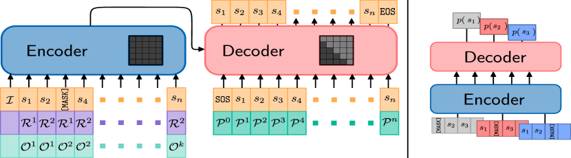
Figure 1: COFS Overview. (Left): The model is a BART-like encoder-decoder model, with a bidirectional encoder and an autoregressive decoder. Note the attention matrices shown in grey. At training time, a permutation $\pi$ permutes the objects in a scene. The encoder receives additional information in the form of Relative Position Tokens $\mathcal{R}^{i}$, and the Object Index Tokens $\mathcal{O}^{i}$. A random proportion of tokens is replaced with a [MASK] token. The decoder is trained with Absolute Position Tokens $\mathcal{P}^{i}$ and performs two tasks - 1. copy-paste: the attributes should be sampled at the proper location 2: mask-prediction: the decoder predicts the actual value of the token corresponding to a [MASK] token in the encoder sequence. (Right): During inference, to measure likelihood, we create a copy of the sequence with each token masked out. The decoder outputs a probability distribution over the possible values of the masked tokens.

Our goal is to design a generative model of object layouts that allows for fine-grained conditioning on individual object attributes. Fine-grained conditioning enables more flexible partial scene specification, for example specifying only the number and types of objects in a scene, but not their positions, or exploring suggestions for plausible objects at given positions in the layout.

Generative model.

We use a transformer-based generative model, as these types of generative models have shown great performance in the current state of the art. Originally, proposed as a generative model for language, transformer-based generative models represents layouts as a sequence of tokens $S=(s_{1},\dots,s_{n})$ that are generated auto-regressively; one token is generated at a time, based on all previously generated tokens:

$$p(s_{i}|S_{<i})=f_{\theta}(S_{<i}),$$ (1)

where $p(s_{i}|S_{<i})$ is the probability distribution over the value of token $s_{i}$, computed by the generative model $f_{\theta}$ given the previously generated tokens $S_{<i}=(s_{1},\dots,s_{i-1})$. We sample from $p(s_{i}|S_{<i})$ to obtain the token $s_{i}$. Each token represents one attribute of an object, and groups of adjacent tokens correspond to objects. More details on the layout representation are described in Section 3.1.

Conditioning.

To condition a transformer-based generative model on a partial sequence $C$, we can replace tokens of $S$ with the corresponding tokens of $C$, giving us the sequence $S^{C}$. This is done after each generation step, so that the probability for the token in each step is conditioned on $S^{C}_{<i}$ instead of $S_{<i}$:

$$p(s_{i}|S^{C}_{<i})=f_{\theta}(S^{C}_{<i}).$$ (2)

Each generated token $s_{i}$ in $S^{C}$ (i.e. tokens that are not replaced by tokens in $C$) needs to have knowledge of the full condition during its generation step, otherwise the generated value may be incompatible with some part of the condition. Therefore, since each generated token $s_{i}$ only has information about the partial sequence $S^{C}_{<i}$, the condition can only be given as start of the sequence:

$$S^{C}=\begin{cases}c_{i}\text{ if }i\leq|C|\\ s_{i}\text{ otherwise}.\end{cases}$$ (3)

Conditioning without permutation invariance.

Typically both the objects and the attributes of the objects in the sequence are consistently ordered according to some strategy, for example based on a raster order of the object positions [24], or on the object size [36]. Therefore, a generative model $f^{\text{ordered}}_{\theta}$ that is only trained to generate sequences in that order cannot handle different orderings, so that in general:

$$f^{\text{ordered}}_{\theta}(S^{C}_{<i})\neq f^{\text{ordered}}_{\theta}(\pi_{o}(S^{C}_{<i})),$$ (4)

where $\pi_{o}$ is a random permutations of the objects in sequence $S_{<i}$. The consistent ordering improves the performance of the generative model, but also presents a challenge for conditioning: the consistent sequence ordering limits the information that can appear in the condition. In a bedroom layout, for example, if beds are always generated before nightstands in the consistent ordering, the layout can never be conditioned on nightstands only, as this would preclude the following tokens from containing a bed.

Permutation invariance for more general conditioning.

Recent work [26] tackles this issue by forgoing the consistent object ordering, and instead training the generator to be approximately invariant to permutations $\pi_{o}$ of objects in the sequence:

$$f_{\theta}(S^{C}_{<i})\approx f_{\theta}(\pi_{o}(S^{C}_{<i})),$$ (5)

This makes generation more difficult, but allows conditioning on arbitrary subset of objects, as now arbitrary objects can appear at the start of the sequence. However, since only objects are permuted and not their attributes, it does not allow conditioning on subsets of object attributes. Permuting object attributes to appear at arbitrary positions in the sequence is not a good solution to obtain a more fine-grained conditioning, as this would make it very hard for the generator to determine which attribute corresponds to which object.

Fine-grained conditioning.

We propose to extend previous work to allow for fine-grained conditioning by using two different conditioning mechanisms, in addition to the approximate object permutation invariance: First, similar to previous work, we provide the condition as partial sequence $C$. To allow conditioning on only a subset of the object attributes, we introduce special mask tokens $\mathcal{M}$ in $C$ that denote tokens that are not constrained by $C$. The constrained sequence $S^{C}$, is then defined as:

$$S^{C}=\begin{cases}c_{i}\text{ if }i\leq|C|\text{ and }c_{i}\neq\mathcal{M}\\ s_{i}\text{ otherwise}.\end{cases}$$ (6)

Second, to provide information about the full condition to each generated token, including those that replace mask tokens, we modify $f_{\theta}$ to use a transformer encoder $g_{\phi}$ that encodes the condition $C$ into a set of feature vectors that each generated token has access to:

$$p(s_{i}|S^{C}_{<i},C)=f_{\theta}(S^{C}_{<i},C^{g})\text{ where }C^{g}=\{g_{\phi}(c_{1},C),\dots,g_{\phi}(c_{|C|},C)\},$$ (7)

where $C^{g}$ is the output of the encoder, a set of encoded condition tokens. We use a standard transformer encoder-decoder setup [34] for $f_{\theta}$ and $g_{\phi}$, implementation details are provided in Section 3.2, and the complete architecture is described in detail in the appendix.

3.1 Layout Representation

Parameters.

We focus on 3D layouts in our experiments. A 3D layout $\mathcal{L}=(\mathcal{I},\mathcal{B})$ is composed of two elements - a top-down representation of the layout boundary $\mathcal{I}$, such as the walls of a room, and a set of $k$ three-dimensional oriented bounding-boxes $\mathcal{B}={\{B_{i}\}}_{i=1}^{k}$ of the objects in the layout. The boundary is given as a binary raster image and each bounding box is represented by four attributes: $B_{i}=(\tau_{i},t_{i},e_{i},r_{i})$, representing the object class, center position, size, and orientation, respectively. The orientation is a rotation about the up-axis, giving a total of 8 scalar values per bounding box. This setup is the same as ATISS.

Layout sequence.

A layout sequence $S$ is defined by randomizing the order of the bounding boxes, concatenating their parameters, and adding special start and stop tokens SOS and EOS to mark the start and the end of a sequence: $S=[\texttt{SOS};B_{\pi_{1}};\dots;B_{\pi_{k}};\texttt{EOS}]$, where $\pi$ is a permutation of the object indices $1,\dots,k$ and $[;]$ denotes concatenation. Note that the objects are permuted in $S$, while the parameters of each object have a consistent order. The condition $C$ for a layout can be any sub-sequence $S_{<i}$ of $S$, where some tokens may be replaced by mask tokens $\mathcal{M}$, leaving them unconstrained. During training and sampling, these tokens are replaced by generated token.

Parameter probability distributions.

The generative model outputs a probability distribution over one scalar component of the bounding box parameters in each step. Similar to previous work [26, 32], we represent probability distributions over continuous parameters, like the center position, size, and orientation, as mixture of $T$ logistic distributions. Probability distributions over the discrete object class $\tau$ are represented as vectors over logits $l_{\tau}$ over discrete choices that can be converted to probabilities with the softmax function.

$$p(b)=\frac{1}{\sum_{i}\pi_{i}}\sum_{i=1}^{T}\alpha_{i}\text{Logistic}(\mu_{i},\sigma_{i}),\qquad\qquad p(\tau)=\text{softmax}(l_{\tau}),$$ (8)

where $b$ is a component of $t_{i}$, $e_{i}$, or $r_{i}$, and $\alpha$, $\mu$, $\sigma$, respectively are the mixture weight, mean and variance of the component logistic distributions. Each probability distribution over a continuous scalar component is parameterized by a $3T$-dimensional vector, and probability distributions over the object class are represented as $n_{\tau}$-dimensional vectors, where $n_{\tau}$ is the number of object classes.

3.2 Implementation

Condition encoder $g_{\phi}$: To encode the condition $C$ into a set of encoded condition tokens $C^{g}$, we use a Transformer encoder with full bidirectional attention. As positional encoding, we provide two additional sequences: object index tokens $\mathcal{O}^{i}$ provide for each token the object index in the permuted sequence of objects; and relative position tokens $\mathcal{R}^{i}$ provide for each token the element index inside the attribute tuple of an object. Since the attribute tuples are consistently ordered the index can be used to identify the attribute type of a token. These sequences are used as additional inputs to the encoder. The encoder architecture is based on BART [19], details are provided in the appendix.

Boundary encoder $g^{\mathcal{I}}_{\psi}$: To allow conditioning on the layout boundary $\mathcal{I}$, we prepend a feature vector encoding of the boundary to the input of the condition encoder, as shown in Figure 1. Similar to ATISS, we use an untrained ResNet-18 [12] to encode a top-down view of the layout boundary into an embedding vector.

Generative model $f_{\theta}$: The generative model is implemented as a Transformer decoder with a causal attention mask. Each block of the decoder performs cross-attention over the encoded condition tokens $C^{g}$. As positional encoding, we provide absolute position tokens $\mathcal{P}$, which provide for each token the absolute position in the sequence $S$. This sequence is used as additional input to the generative model. The output of the generative model in each step is one of the parametric probability distributions described in Eq. 8. Since the probability distributions for discrete and continuous values have a different numbers of parameters, we use a different final linear layer in the generative model for continuous and discrete parameters. Similar to the encoder, the architecture of the generative model is based on BART [19].

Training: During training, we create a ground truth sequence $S^{\text{GT}}$ with randomly permuted objects. We generate the condition $C$ as a copy of $S^{\text{GT}}$ and mask out a random percentage of the tokens by replacing them with the mask token $\mathcal{M}$. The boundary encoder $g^{\mathcal{I}}_{\psi}$, the condition encoder $g_{\phi}$ and the generative model $f_{\theta}$ are then trained jointly, with the task to generate the full sequence $S^{\text{GT}}$. For unmasked tokens in $C$, this is a copy task from $C$ to the output sequence $S$. For masked tokens, this is a scene completion task. We use the negative log-likelihood loss between the predicted probabilities $p(s_{i})$ and ground truth values $s^{\text{GT}}_{i}$ for tokens corresponding to continuous parameters, and the cross-entropy loss for the object category $\tau$. The model is trained with teacher-forcing.

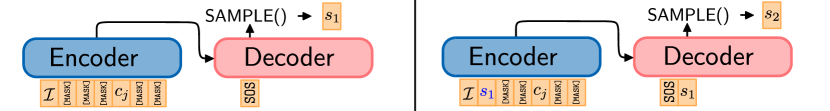
Figure 2: Sampling Strategy. (Left): We start out with a sequence of all [MASK] tokens on the encoder, and the SOS token on the decoder. Conditions, if any, are specified by replacing the [MASK] with the desired value of the attribute in the sequence. Sampling is performed autoregressively. (Right): After a token has been sampled, both the encoder and decoder sequences are updated, and atuoregressive generation continues.

Sampling: We generate a sequence auto-regressively, one token at a time, by sampling the probability distribution predicted by the generative model (as defined in Eq. 7) in each step. We use the same model for both conditional and unconditional generation. For unconditional generation, we start with a condition $C$ where all tokens are mask token $\mathcal{M}$. To provide more complete information about the partially generated scene to the encoded condition tokens $C^{g}$, we update the condition $C$ after each generation step by replacing mask tokens with the generated tokens. Empirically, we observed that this improves generation performance. An illustration of this approach is shown in Fig. 2. The function SAMPLE samples from the probability distributions described in Eq. 8.

Once a layout has been generated, we can populate the bounding boxes with objects from the dataset. For each bounding box, we pick the object of the given category $\tau$ that best matches the size of the bounding box. In the supplementary, we will present an ablation of the tokens $\mathcal{O}^{i}$, $\mathcal{R}^{i}$, and $\mathcal{P}$ that we add to the conditional encoder and generative model.

4 Results

Table 2: Comparison on Unconditional Generation: We provide floorplan boundaries from the Ground Truth as an input to the methods and compare the quality of generate scenes. We measure the CAS at a resolution of $256\times 256$.We retrain the ATISS model and report the new numbers. The retrained model is called ATISS^∗. The KL-Divergence follows from [30] and is the categorical KL-divergence between the distribution of classes in the GT and the layouts synthesised by our method.

	CAS $\times 10^{2}$($\downarrow$)				KL-Divergence $\times 10^{3}$ ($\downarrow$)
	Bedroom	Living	Dining	Library	Bedroom	Living	Dining	Library
FastSynth	88.3	94.5	93.5	81.5	6.4	17.6	51.8	43.1
SceneFormer	94.5	97.2	94.1	88.0	5.2	31.3	36.8	23.2
ATISS∗	61.1	76.4	69.1	61.77	8.6	14.1	15.6	10.1
Ours	61.0	78.9	76.1	66.2	5.0	8.1	9.3	6.7

Boundary

GT

ATISS

Ours

\begin{overpic}[width=433.62pt,trim=0.0pt 501.87498pt 0.0pt 602.25pt,clip]{figures/unconstrained/LivingDiningRoom-6844_gt_orthopng.jpg} \end{overpic}

\begin{overpic}[width=433.62pt,trim=0.0pt 501.87498pt 0.0pt 602.25pt,clip]{figures/unconstrained/LivingDiningRoom-6844_atiss_orthopng.jpg} \end{overpic}

\begin{overpic}[width=433.62pt,trim=0.0pt 501.87498pt 0.0pt 602.25pt,clip]{figures/unconstrained/LivingDiningRoom-6844_orthopng.jpg} \end{overpic}

\begin{overpic}[width=433.62pt,trim=531.98749pt 381.42499pt 100.37498pt 602.25pt,clip]{figures/unconstrained/LivingDiningRoom-20487_gt_orthopng.jpg} \end{overpic}

\begin{overpic}[width=433.62pt,trim=531.98749pt 381.42499pt 100.37498pt 602.25pt,clip]{figures/unconstrained/LivingDiningRoom-20487_atiss_orthopng.jpg} \end{overpic}

\begin{overpic}[width=433.62pt,trim=531.98749pt 381.42499pt 100.37498pt 602.25pt,clip]{figures/unconstrained/LivingDiningRoom-20487_orthopng.jpg} \end{overpic}

\begin{overpic}[width=433.62pt,trim=552.0625pt 602.25pt 602.25pt 552.0625pt,clip]{figures/unconstrained/dinner_orthopng.jpg} \end{overpic}

\begin{overpic}[width=433.62pt,trim=552.0625pt 602.25pt 602.25pt 552.0625pt,clip]{figures/unconstrained/DiningRoom-10302_atiss_orthopng.jpg} \end{overpic}

\begin{overpic}[width=433.62pt,trim=552.0625pt 602.25pt 602.25pt 552.0625pt,clip]{figures/unconstrained/DiningRoom-10302_orthopng.jpg} \end{overpic}

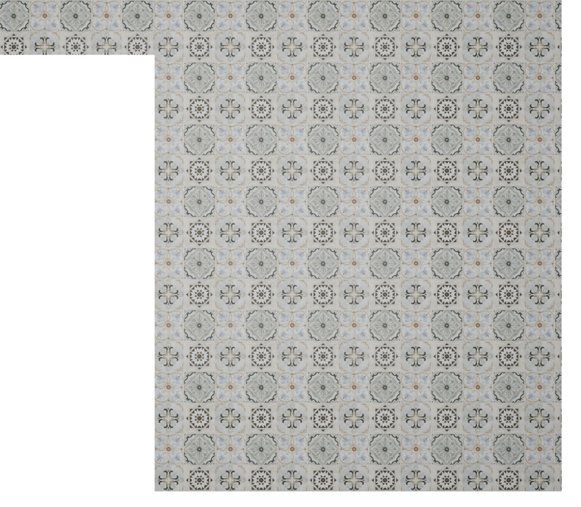
\begin{overpic}[width=433.62pt,trim=531.98749pt 381.42499pt 301.125pt 602.25pt,clip]{figures/unconstrained/LivingDiningRoom-2648_gt_orthopng.jpg} \end{overpic}

\begin{overpic}[width=433.62pt,trim=531.98749pt 381.42499pt 301.125pt 602.25pt,clip]{figures/unconstrained/LivingDiningRoom-2648_atiss_orthopng.jpg} \end{overpic}

\begin{overpic}[width=433.62pt,trim=531.98749pt 381.42499pt 301.125pt 602.25pt,clip]{figures/unconstrained/LivingDiningRoom-2648_orthopng.jpg} \end{overpic}

Figure 3: Scene generation from scratch: We compare generated scenes from GT, ATISS, and our model. Both ATISS and our model are conditioned on the floorplan boundary (first column). In contrast to ATISS, we can see that our model consistently creates plausible layouts within the floorplan boundary while avoiding unnatural object intersections. These are results on the challenging Living (rows 1,3) and Dining (row 2,4) categories. Additional results can be found in the supplementary. (Best viewed zoomed in, on a computer display)

4.1 Experimental Setup

Datasets: We train and evaluate our model on the 3D-FRONT dataset. It consists of of about $10k$ indoor scenes created by professional designers. We follow ATISS preprocessing which removes a few problematic scenes that have intersections between objects, or mislabeled objects, or scenes that have extremely large or small dimensions. For further details on the preprocessing, we refer the reader to ATISS [26]. We train on the following classes of rooms - Bedroom, Library, Dining, Living. We closely follow the preprocessing step of ATISS, yielding approximately $6k$, $0.6k$, $3k$ and $2.6k$ scenes for Bedroom, Library, Dining, Living respectively. These classes have substantially different numbers of layouts and numbers of objects per layout.

Hyperparameters: We implement our models in PyTorch [27] 1.7.0. We use standard transformer blocks for the encoder and decoder except that the ReLU activation is replaced with GeLU [13]. We use 4 encoder layers and 4 decoder layers, with a hidden dimension of 256 and 4 attention heads yielding a query vector of dimension 64. We use a batch size of 128 sequences and train on a single nVIDIA A100 GPU with the AdamW [21] optimizer which we found to be more stable than Adam [16]. We use weight decay of 0.001 and clip the gradient norm to be a maximium of 30. We found that the networks begins to overfit very early, especially for classes other than Bedroom, because of the scarcity of data. Thus, for training networks on other classes, we pre-train on the Bedroom class, and then reuse those weights as initialization. We do not use any form of learning rate scheduling as our experiments did not suggest significant performance gains. We train for 1000 epochs and use early stopping.

Baselines: Our main comparison is with respect to ATISS, as they are the only other method that considers the layout generation problem in a permutation invariant set-generation setting. We show that our model is competitive with ATISS and outperforms it on certain metrics. Moreover, we subsume all functionality of ATISS, including partial scene completion and outlier detection. Unlike ATISS, our model allows for fine-grained conditioning on arbitrary object parameters.

ATISS does not provide pretrained models, hence we train their models using the official code and match their training settings as closely as possible. Further, we compare to previous state-of-the art methods, FastSynth [30] and SceneFormer [37] quantitatively.

Metrics: Our metrics mostly derive from [30, 26]. Following, [30], we report the KL-divergence between the distribution of the classes of generated objects and the distribution of classes of the objects in the test set. We further report the Classification Accuracy Score (CAS) [26]. We render the the populated layout from a top-down view using an orthographic camera at a resolution of $256\times 256$. We report the FID computed between these rendered top down images of sampled layouts and the renders of the ground truth layouts.

4.2 Applications

In this section, we discuss the application of our model on multiple interactive tasks. We show that our formulation a) can perform the same tasks as existing models and b) additionally enables fine-grained conditioning on arbitrary sequence subsets, like individual object parameters.

Scene Completion: In order to perform scene completion, we prepend both $S$ and $C$ with the tokens of the objects that already exist in the scene. Examples are shown in Figure 4. We can see that our method successfully generates plausible room layouts that respect the condition shown in the top row.

\begin{overpic}[width=433.62pt,trim=642.4pt 602.25pt 602.25pt 903.37498pt,clip]{figures/completions/partial_1_westpng.jpg} \end{overpic}

\begin{overpic}[width=433.62pt,trim=602.25pt 602.25pt 602.25pt 762.84999pt,clip]{figures/completions/partial_2_eastpng.jpg} \end{overpic}

\begin{overpic}[width=433.62pt,trim=602.25pt 602.25pt 602.25pt 702.625pt,clip]{figures/completions/partial_3_eastpng.jpg} \end{overpic}

\begin{overpic}[width=433.62pt,trim=552.0625pt 702.625pt 501.87498pt 501.87498pt,clip]{figures/completions/partial_4_northpng.jpg} \end{overpic}

\begin{overpic}[width=433.62pt,trim=501.87498pt 602.25pt 501.87498pt 552.0625pt,clip]{figures/completions/partial_5_northpng.jpg} \end{overpic}

\begin{overpic}[width=433.62pt,trim=602.25pt 702.625pt 602.25pt 552.0625pt,clip]{figures/completions/partial_6_northpng.jpg} \end{overpic}

\begin{overpic}[width=433.62pt,trim=642.4pt 602.25pt 602.25pt 903.37498pt,clip]{figures/completions/completed_1_westpng.jpg} \end{overpic}

\begin{overpic}[width=433.62pt,trim=602.25pt 602.25pt 602.25pt 762.84999pt,clip]{figures/completions/completed_2_eastpng.jpg} \end{overpic}

\begin{overpic}[width=433.62pt,trim=602.25pt 602.25pt 602.25pt 702.625pt,clip]{figures/completions/completed_3_eastpng.jpg} \end{overpic}

\begin{overpic}[width=433.62pt,trim=552.0625pt 702.625pt 501.87498pt 501.87498pt,clip]{figures/completions/complete_4_northpng.jpg} \end{overpic}

\begin{overpic}[width=433.62pt,trim=501.87498pt 602.25pt 501.87498pt 552.0625pt,clip]{figures/completions/complete_5_northpng.jpg} \end{overpic}

\begin{overpic}[width=433.62pt,trim=602.25pt 702.625pt 602.25pt 552.0625pt,clip]{figures/completions/complete_6_northpng.jpg} \end{overpic}

Figure 4: Partial Scene Completion: We show qualitative visualizations for the scene completion task. The generated layouts all respect the condition they were generated with (top row) and are all plausible room layouts.

Outlier Detection: To estimate the likelihood of each token, we follow [31] and replace the token at $i$th position with [MASK]. This can be performed in parallel by creating a batch in which only one element is replaced with [MASK]. This is shown in Fig. 1. The likelihood of one bounding box then is the product of likelihoods of all element of the bounding box. Objects with low likelihood can then be resampled. Based on user constraints, only one parameter may be changed as we allow for arbitrary conditioning as explained in the next section.

\begin{overpic}[width=433.62pt,trim=501.87498pt 501.87498pt 501.87498pt 501.87498pt,clip]{figures/outlier/bad_last_sepng.jpg} \end{overpic}

\begin{overpic}[width=433.62pt,trim=501.87498pt 501.87498pt 501.87498pt 501.87498pt,clip]{figures/outlier/bad1_sepng.jpg} \end{overpic}

\begin{overpic}[width=433.62pt,trim=100.37498pt 301.125pt 401.49998pt 702.625pt,clip]{figures/outlier/bad2_eastpng.jpg} \end{overpic}

\begin{overpic}[width=433.62pt,trim=401.49998pt 301.125pt 401.49998pt 652.4375pt,clip]{figures/outlier/bad3_sepng.jpg} \end{overpic}

\begin{overpic}[width=433.62pt,trim=100.37498pt 200.74998pt 200.74998pt 501.87498pt,clip]{figures/outlier/bad4_nepng.jpg} \end{overpic}

\begin{overpic}[width=433.62pt,trim=100.37498pt 401.49998pt 401.49998pt 552.0625pt,clip]{figures/outlier/bad5_nwpng.jpg} \end{overpic}

\begin{overpic}[width=433.62pt,trim=501.87498pt 501.87498pt 501.87498pt 501.87498pt,clip]{figures/outlier/good_last_sepng.jpg} \end{overpic}

\begin{overpic}[width=433.62pt,trim=501.87498pt 501.87498pt 501.87498pt 501.87498pt,clip]{figures/outlier/good1_sepng.jpg} \end{overpic}

\begin{overpic}[width=433.62pt,trim=100.37498pt 301.125pt 401.49998pt 702.625pt,clip]{figures/outlier/good2_eastpng.jpg} \end{overpic}

\begin{overpic}[width=433.62pt,trim=401.49998pt 301.125pt 401.49998pt 652.4375pt,clip]{figures/outlier/good3_sepng.jpg} \end{overpic}

\begin{overpic}[width=433.62pt,trim=100.37498pt 200.74998pt 200.74998pt 501.87498pt,clip]{figures/outlier/good4_nepng.jpg} \end{overpic}

\begin{overpic}[width=433.62pt,trim=100.37498pt 401.49998pt 401.49998pt 552.0625pt,clip]{figures/outlier/good5_nwpng.jpg} \end{overpic}

Figure 5: Outlier detection: Our model can utilize bidirectional attention to reason about unlikely arrangements of furniture. We can then sample new attributes that create a more likely layout. Top row: An object is perturbed to create an outlier (highlighted in blue). Bottom row: The object can be identified by its low likelihood, and new attributes sampled which place it more naturally. Please zoom in for best viewing.

Arbitrary Conditioning: To condition on an arbitrary sub-set of object attributes, we can construct a condition $C$ that is filled with [MASK] tokens, i.e. a fully unconstrained setting, and then only replace the tokens in $C$ corresponding to the attributes we want to constrain with constraint values. The non-mask tokens do not need to be contiguous in $C$. Any subset of $C$, for example only object class attributes or only object locations, can be used as unmasked condition. Given such a constraint $C$, the generator proceeds as described in Section 3.2 and fills in all mask tokens with generated values. The encoder allows each generation step to have full knowledge of the condition $C$. See Fig. 6 for examples. To the best of our knowledge, ours is the first model that allows for this form of conditioning without imposing an order on the generation of parameters.

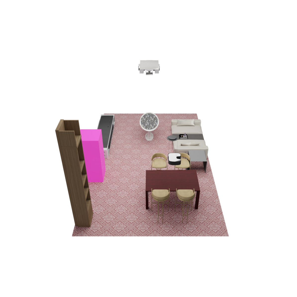
\begin{overpic}[width=433.62pt,trim=451.68748pt 501.87498pt 501.87498pt 451.68748pt,clip]{figures/conditioning/cabinets_northpng.png} \end{overpic}

\begin{overpic}[width=433.62pt,trim=451.68748pt 501.87498pt 501.87498pt 451.68748pt,clip]{figures/conditioning/condition/chair_northpng.png} \end{overpic}

\begin{overpic}[width=433.62pt,trim=451.68748pt 501.87498pt 501.87498pt 451.68748pt,clip]{figures/conditioning/chairs_northpng.png} \end{overpic}

Figure 6: Arbitrary conditioning: We constrain the location of the next object to be sampled. The location is highlighted in pink. We sample location after the class. In a normal autoregressive model, we would not be able to constrain on the location. The bidirectional attention in the encoder allows the network to generate current tokens based on future tokens. In this example, the network automatically infers the proper class and size and even matches the style of the chairs in the example on the left.

5 Conclusions

We proposed a new framework to produce layouts with auto-regressive transformers with arbitrary conditioning information. While previous work was only able to condition on a set of complete objects, we extend this functionality and also allow for conditioning on individual attributes of objects. Our framework thereby enables several new modeling applications that cannot be achieved by any published framework.

Societal Impact.

We do not expect any negative social impact that is directly linked to our work. We do acknowledge possible concerns about the energy consumption of training auto-regressive transformers.

Limitations and Future Work.

Our work inherits some limitations of auto-regressive models (or even generative models in general) in that we require long training times and that setting up the code is laborious, time-consuming and error-prone. In addition, it requires significant expert knowledge in training transformers. We will therefore release the code upon acceptance. Another limitation of the work is that all objects need to have the same number of attributes. An open challenge for future work is to extend our approach to layouts where each object is described by a token sequence of variable length. Further, we would like to work on scaling auto-regressive models to much larger sequences, e.g., by using hierarchical auto-regressive models. In future, we would also like to explore parallel sampling strategies to sidestep the slow autoregressive generation process.

Table 3: Comparison on Synthesis Time: We compare the time required to synthesize a single scene for different categories. Our model outperforms all other models on this metric, and is competitive on FID in comparison to ATISS. Our model achieves this while being parameter efficient. We only have about half the parameters of the next closest competitor. About 10m of these parameters come from the ResNet-18 encoder.

	Synthesis Time ($\downarrow$)				FID ($\downarrow$)				Params ($\downarrow$)
	Bedroom	Living	Dining	Library	Bedroom	Living	Dining	Library
FastSynth	13193.77	30578.54	26596.08	10813.87	88.1	66.6	58.9	86.6	38.1
SceneFormer	849.37	731.84	901.17	369.74	90.6	68.1	60.1	89.1	129.29
ATISS	102.38	201.59	201.84	88.24	73.0	43.32	47.66	75.34	36.05
Ours	33.69	77.37	76.75	29.32	73.2	35.9	43.12	75.72	19.44

6 Acknowledgements

We would like to thank Visual Computing Center (VCC), KAUST for support, gifts from Adobe Research and the UCL AI Centre.

COFS: Controllable Furniture layout Synthesis
Supplementary Material

Appendix A Detailed Architecture and Training Setup

We base our architecture on ATISS [26] in order to ensure a fair comparison to our closest competitor, using the same underlying library [15]. Consequently, most of the building blocks are shared. However, we would like to point out major differences in this section.

Layout sequence:

During training, we construct the sequence $S$ corresponding to the layout by arranging the object bounding boxes in a random order with a permutation $\pi$ and concatenating their bounding box attributes as individual tokens.

$$s_{2} =\tau_{\pi_{1}},\;s_{3}=(\tau_{\pi_{1}})_{x},\;s_{4}=(\tau_{\pi_{1}})_{y},\;s_{5}=(\tau_{\pi_{1}})_{z},\;s_{6}=(e_{\pi_{1}})_{x},\;\cdots\;s_{9}=\tau_{\pi_{2}}\;\cdots\;$$ (9)

$$s_{1} =\texttt{SOS},\;s_{k}=\texttt{EOS}$$

where $\tau_{\pi_{1}}$ and $(t_{\pi_{1}})_{x}$ represent the class and $x-$translation of the first object after permutation, $\tau_{\pi_{2}}$ represents the class of the second object after permutation and so on.

Object attributes are always flattened the same way in our implementation, although in principle the attribute order can itself be permuted. We use the same attribute order for ease of implementation.

Embeddings:

We described how we generate embeddings for the tokens in $C$ and $S$. We use a learnable matrix $E_{class}$ of dimension $n_{\tau}\times 256$ to encode the type $\tau_{i}$, with each row corresponding to one class. We use an additional [MASK] class. For the other attributes of translation ($t_{i}$), size ($e_{i}$) and rotation ($r_{i}$), we use sinuosoidal positional encodings [34, 26] with 128 levels ($L=128$). We call these embeddings $\gamma$:

$$\gamma(b)=\begin{cases}(\sin(2^{0}\pi b),\cos(2^{0}\pi b),\dots,\sin(2^{L-1}\pi b),\cos(2^{L-1}\pi b))&\qquad\text{if \quad}b\in\{t,e,r\}\\ E_{class}[\tau,:]&\qquad\text{if \quad}b\in\{\tau\}\end{cases}$$ (10)

For the encoder, the embeddings of $\mathcal{R}^{i}$ are a learned matrix $E_{r}$ of dimension $8\times 256$. Each row corresponds to a different type of attribute - one for type, 3 each for translation and size, and one for the rotation. The embedding of $\mathcal{O}^{i}$ are again a learned matrix $E_{o}$ of dimension $k\times 256$, where $k$ is the maximum number of objects. For the decoder, the embeddings of $\mathcal{P}^{i}$ are also a learned matrix $E_{p}$ of size $n\times 256$. The final embeddings are the sum of the corresponding embeddings:

$$\gamma_{e}(b_{i}) =\gamma(b_{i})+E_{r}[\mathcal{R}^{i},:]+E_{o}[\mathcal{O}^{i},:]$$ (11)

$$\gamma_{d}(b_{i}) =\gamma(b_{i})+E_{p}[\mathcal{P}^{i},:]$$

where $\gamma_{e}$ and $\gamma_{d}$ are the encoder and decoder embeddings respectively.

Optimizer:

We use the PyTorch [27] implementation of the AdamW [21] optimizer with the default parameters for our model with a constant learning rate of $10^{-4}$ and weight decay set to $10^{-3}$. We linearly warmup the learning rate for 2000 steps. In addition, we found gradient clipping to be necessary to ensure convergence. We set the maximum gradient norm to be $30$. Empirically, we found that setting the gradient norm to be low led to slower convergence.

We train with a batch size of 128, and train for 1000 epochs. We perform validation every 5 epochs. We save the model with the best performance on the validation set. We use random rotation augmentation by randomly rotating each scene between 0 and 360 degrees.

We wish to clarify that while we used the AdamW optimizer for our model, we used the vanilla Adam optimizer for ATISS, as described in [26].

Parameter Probability Distributions:

We need to predict object attributes from the final transformer decoder outputs. To this end, we use use MLPs to go from the embedding dimension to the parameters of the distribution describing the attributes. For the class $\tau$, we use a linear layer from the embedding dimension to the number of classes. For the other attributes, we use MLPs with one-input layer ($256,512$), one hidden-layer ($512,256$), and one output-layer ($256,30$) and ReLU activations. The output size reflects that we use a mixture distribution with 10 components, and each component-distribution is parameterized by 3 values.

Transfer Learning:

The datasets Living, Dining, Library are much smaller compared to the Bedroom dataset. Thus, we use a transfer learning approach, where we first train on the Bedroom dataset, and use those weights as an initialization, when training on the smaller datasets. This reduces the training time significantly, as well as combats overfitting on the smaller datasets.

We note that the datasets have a slightly different number of classes, thus any weights associated with the number of classes are not transferred, but instead sampled from a Normal Distribution, with mean $0$ and standard deviation $0.01$.

A.1 Metrics

The evaluation protocol follows ATISS closely, but we describe it here for the sake of completeness.

To compute the FID, we render both the ground-truth and generated layouts from a top-down view into a $256\times 256$ images with an orthographic camera using Blender v3.1.0 [6]. Following ATISS, the FID is computed using the code from Parmar et al. [25]  We will release the .blend-file used for rendering upon acceptance. To compute the Classifier Accuracy Score (CAS), we use an AlexNet [17]  model pretrained on ImageNet[7] to classify the orthographic renderings as real or fake. The Synthesis Time numbers for the competing models are lifted from ATISS [26]. We train our models on an nVIDIA A100 GPU. To ensure fair comparison to the numbers in ATISS, we ran inference on a GTX 1080 GPU which is the same GPU used in [26]. To compute the KL-divergence, we simply create a histogram of object categories in the generated layouts $g_{i}$ and the ground-truth $gt_{i}$, where $1\leq i\leq n_{class}$ and use the the formula for the categorical KL-Divergence:

$$KL(gt_{i}\|g_{i})=\sum_{i}gt_{i}\log\left(\frac{gt_{i}+\epsilon}{g_{i}+\epsilon}\right)$$ (12)

where $\epsilon=10^{-6}$ is a small constant for numerical stability.

We use the same train-val-test splits as ATISS. To compute the aforementioned metrics, we generate layouts for all floorplans in the test-set and compare each with the corresponding ground-truth layout.

Appendix B 3D-Front Dataset

To the best of our knowledge, the 3D-Front [11] dataset is the largest collection of indoor furniture layouts in the public domain. Its large scale is obtained, in part, by employing a semi-automatic pipeline, where a machine-learning system places the objects roughly, and an optimization step [38] refines the layouts further to conform to design standards. The only human involvement is verification that the layouts are valid - do not have object intersections, objects that block doors, etc. However, in our exploration, we find several inconsistencies still remain in the dataset. We mention a few - nightstands intersecting their nearest beds, nightstands obstructing wardrobes, chairs intersecting their closest tables, and chairs that face in the wrong directions. We point out a few of these examples in Fig. 7.

Our method, like other data-driven methods, learns the placement of objects from data. Thus, any errors in the ground-truth data itself would also show up in the sampled layouts. This is true, especially for Bedroom dataset, where the sampled nightstands often end up intersecting with beds.

Figure 7: We show a few examples of inconsistencies in the 3D-FRONT dataset. Top: Camera placement in 3D-Front layouts. Center: The corresponding regions show errors in the ground-truth data. Left: Chairs facing and intersecting a shelf. Right: Chairs in the correct orientation, but intersecting with a table. Bottom: Some more ground-truth errors. (From Left to Right:) Intersection. Blocking. Wrong Orientation and Intersection. Wrong Orientation.

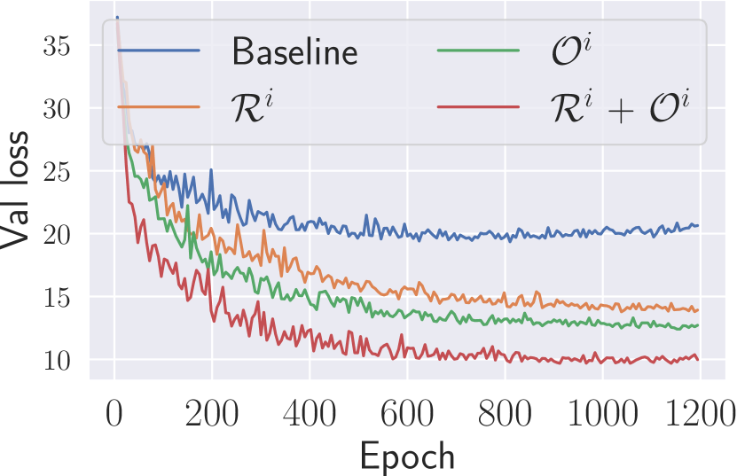
(a) Adding additional tokens helps the decoder to better align the input and the output.

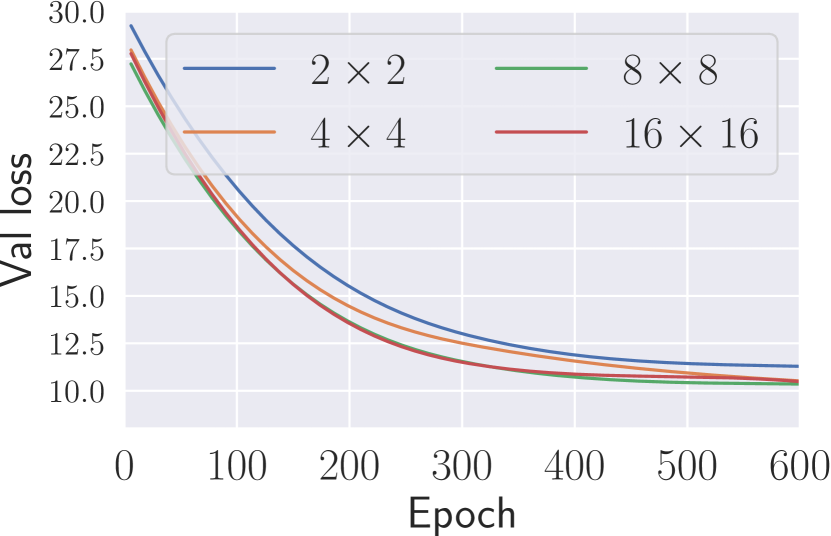
(b) The smaller models perform worse, but adding more layers does not yield large correspondingly larger gains.

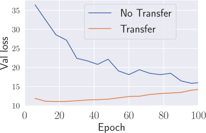
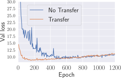
(c) Left: Transfering weights on the Library dataset. Right: Transferring weights on the Living dataset.

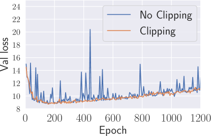
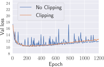
(d) Left: Gradient clipping applied on the Dining dataset. Right: Gradient clipping applied on the Living dataset.

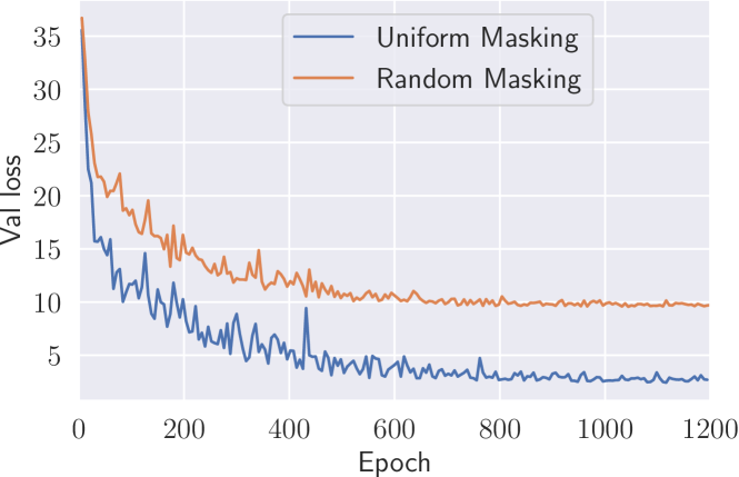
(e) Using a uniform masking ratio of $0.15$ shows good performance in terms of NLL, but is unable to sample owing to large distribution shift between training and inference.

Figure 8: Ablation Studies We show the validation losses for the different architectural choices we make.

Appendix C Ablations

In this section, we justify our design choices by conducting an ablation study. We train our model under different settings on the Bedroom dataset, unless specified otherwise, and use the validation loss, the Negative Log-Likelihood (NLL) as the metric to judge performance. This is because we empirically found the validation loss to correlate directly with sample quality. In particular, we ablate the choice of our position encodings, the number of layers and training with gradient clipping. We also include a discussion of the masking strategy and transfer learning.

C.1 Position Encodings

We consider the input conditioning to be a set. In contrast, the output is a sequence. Thus, the model needs additional information to align the input and the output . We use object index tokens $\mathcal{O}^{i}$ and the relative position tokens $\mathcal{R}^{i}$ to provide this additional information.

During training, the objects themselves are permuted. The intuition is that $\mathcal{O}^{i}$ injects information about how early or late each object must appear in the output sequence. However, this information alone is not enough to disambiguate where each of the attributes of the object must appear. Hence, we also add $\mathcal{R}^{i}$ to the object attribute embeddings. Together, these embeddings localize the position of the attribute in the output sequence, given the current permutation.

In Fig. 8(a), we progressively add our embeddings to the Baseline model which is the model without any positional encodings on the encoder. It is clear that using our embeddings helps the model better align the set-input and the sequence-output. While each of $\mathcal{O}^{i}$ and $\mathcal{R}^{i}$ roughly align the input and the output, it is only when using both the embeddings that the model can precisely locate the actual position of tokens in the output sequence.

C.2 Number of Layers

For all the experiments in the main paper, we used 4 transformer layers in both the encoder and the decoder. In Fig. 8(b), we show how the model performance scales with scaling the number of layers. We see that the performance correlates strongly with the number of layers. However, the performance gains become marginal when going from 4 to 8 layers or 8 to 16 layers. These larger models take longer to train and sample from. We believe our 4 layer models provide a good compromise between performance and speed.

Note that the values in Fig. 8(b) are smoothed by an interpolating spline to highlight the general trend.

C.3 Gradient Clipping

We found that the validation loss oscillated considerably during training. Upon further investigation, we noticed that the gradients norms tended to be unusually large, especially for the last layers in the parameter generating MLPs. Thus, we train the final networks with gradient clipping. Surprisingly, we found that even without gradient clipping, if we retain the model with the best NLL on the validation set, the performance is the same. However, with gradient clipping, we found the training curves to be much smoother (Fig. 8(d)). Consequently, we were able to perform validation at less frequent intervals to select the best performing model, which sped up training.

C.4 Masking Strategy

MaskGIT [3] find that using a robust masking strategy is important, as the usual $15\%$ masking leads to a distribution shift between training and sampling. We see in Fig. 8(e) that masking with a uniform ratio of $15\%$ leads to better NLL as the network is more confident in it’s predictions. But we found out that the we could not sample from such a trained network, as it would output a stop token after only generating a few objects, which intuitively makes sense, as the network would only see a few mask tokens during training.

C.5 Transfer Learning:

We plot the validation loss in Fig. 8(c) on the Library and Living datasets under two configurations - No Transfer, where the models are trained from scratch and Transfer, where the model is first trained on the Bedroom dataset and these weights are used as initialization for training on the target dataset. We make a few observations: 1. The models begin to overfit fairly early. For the Bedroom dataset, the loss contiues to fall until epoch 1200, but in the No Transfer configuration for the Library dataset, we see overfitting at epoch 150 and for the Living dataset, at epoch 600. We hypothesize that this is due to the small size of these datasets compared to the Bedroom dataset. 2. The No Transfer configuration has a higher (worse) NLL as compared to the Transfer configuration, even when trained for longer.

These observations led us to use the Transfer configuration for the Library, Living and Dining datasets.

Appendix D Sampling Details

We highlight the difference between our sampling algorithm and the standard conditional sampling algorithm in this section. These differences are highlighted in blue in Alg. 2. The primary difference is that in our sampling algorithm, a forward pass is made through the decoder every time a new token is sampled. This token then replaces the corresponding [MASK] token in both $C$ and $S$.

In addition, our algorithm runs for a fixed number of iterations (until all [MASK] tokens are replaced) compared to the standard algorithm which terminates when an EOS token is generated. This is both an advantage and a drawback - it is an advantage in the sense that a user can implicitly specify the number of objects by specifying the number of [MASK] tokens. It is a drawback in that the number of objects must be known before sampling can proceed.

D.1 A Sampling Trick

For our outlier detection examples, we use a simple trick - if there is only a single object to be sampled, we can create a permutation so that the [MASK] tokens of the object to be sampled are toward the end of the sequence in $C$ and $S$. With this permutation we only have to make forward passes beginning from the first masked token. All the tokens before the first masked token can simply be copied. This leads to faster sampling.

Algorithm 1 Standard Cond. Sampling

1:$C=(c_{i})_{i=1}^{k}$, $S=(\texttt{SOS}),s=\phi$

2:${C^{g}=g_{\phi}([\mathcal{I},C])}$ $\triangleright$ Only performed once

3:while $s\neq\texttt{EOS}$ do

4:    $s=\textsf{SAMPLE}(f_{\theta}(S_{<i},C^{g}))$

5:    $S\textsf{.append($s$)}$ $\triangleright$ $C$ not updated

6:end while

7:return $S$

Algorithm 2 Our Sampling

1:$\mathcal{I}$, $C=(\texttt{[MASK]})_{i=1}^{k}$, $S=(\texttt{SOS})$

2:for $i\leftarrow 1$ to $k$ do

3:    ${\color[rgb]{0,0,1}C^{g}=g_{\phi}([\mathcal{I},C])}$

4:    $s=\textsf{SAMPLE}(f_{\theta}(S_{<i},C^{g}))$

5:    ${\color[rgb]{0,0,1}C[i]=s},\;S\textsf{.append($s$)}$

6:end for

7:return $S$

In all our experiments, we set the number of objects to be sampled to be the same as the number of objects in the ground-truth layout associated with the particular floorplan boundary.

Appendix E Arbitrary Conditioning

We first recap the sampling strategy of ATISS.

$$c_{\theta}:\mathbb{R}^{64} \rightarrow\mathbb{R}^{C} \hat{\mathbf{q}}\mapsto\hat{\mathbf{c}}$$ (13)

$$t_{\theta}:\mathbb{R}^{64}\times\mathbb{R}^{L_{c}} \rightarrow\mathbb{R}^{3\times 3\times K} (\hat{\mathbf{q}},\lambda(\mathbf{c}))\mapsto\hat{\mathbf{t}}$$ (14)

$$r_{\theta}:\mathbb{R}^{64}\times\mathbb{R}^{L_{c}}\times\mathbb{R}^{L_{t}} \rightarrow\mathbb{R}^{1\times 3\times K} (\hat{\mathbf{q}},\lambda(\mathbf{c}),\gamma(\mathbf{t}))\mapsto\hat{\mathbf{r}}$$ (15)

$$s_{\theta}:\mathbb{R}^{64}\times\mathbb{R}^{L_{c}}\times\mathbb{R}^{L_{t}}\times\mathbb{R}^{L_{r}} \rightarrow\mathbb{R}^{3\times 3\times K} (\hat{\mathbf{q}},\lambda(\mathbf{c}),\gamma(\mathbf{t}),\gamma(\mathbf{r}))\mapsto\hat{\mathbf{s}}$$ (16)

These equations say the following: From a query vector $\hat{\mathbf{q}}$, the model predicts a class. From the query and class, the model predicts the translation. From the query, class, and translation, the model predicts a rotation, and so on. This means that in ATISS, future attributes cannot affect the distribution of previous attributes. When conditioning, we can specify the class and then sample a translation, but we cannot specify a translation and let the model infer the most likely class for that given translation.

In contrast, COFS has bidirectional attention on the encoder side, enabling us to specify any subset of object attributes. This is done by replacing the [MASK] token corresponding to the object attribute by its actual value in $C$. The copy-paste objective ensures that the same attribute will be sampled at the desired location by the decoder. The mask-predict objective trains the model to get the most-likely attributes for the unspecified tokens.

We describe the process using the following example: We start out with a layout, shown in Fig. 10(a). If we mask out the table in cyan (Fig. 10(b), and sample unconditionally, we get another similar table (Fig. 10(c)). We now wish to have some control over the generation process.

We now mask out a different object - stool in the upper left corner. We have masked out a single object, thus we have 8 [MASK] tokens. Our sequences $C$ and $S$ look like Fig. 10(d). If we want to specify the position of the next object, we simply set the token corresponding to position-attribute of the next object in $C$ - $c_{i}$ to the value we want. We show a few examples of this type of conditioning in Fig. 10(f) and Fig. 10(g). In the rest of the figures, before beginning sampling, we set the class tokens. We see that the generated layouts follow the condition, while also generating plausible layouts, even if the classes of conditioning objects never occur together. As an example, there are only 5 examples of bedrooms with two beds, yet our model is able to reason about the placement of such challenging layouts in Row 5.

We further see that the model is able to place other objects in such a manner that the constrained objects can still satisfy their constraints. In Row 4, we see that when we constrain the angle of the bed, the other objects move in tandem to create a plausible layout.

Appendix F Limitations and Discussion

We now discuss limitations of our model. The first is related to our simple object retrieval scheme based only on bounding box sizes. This often leads to stylistically different objects in close proximity even if the bounding box dimensions are slightly different. We show such an example in Fig. 9(left). The second is related to the training objective of the model - we only consider the cross entropy/NLL. Thus, the network does not have explicit knowledge of design principles such as non-intersection, or object co-occurrence. This means that the model completely relies on the data being high-quality to ensure such output. We highlighted the fact that certain scenes in the dataset have problematic layouts, and our method cannot filter them out. We show an example of intersections in Fig. 9(center). Thirdly, the the performance on the Living and Dining datasets is not as good as the other classes, which is clear from the CAS scores. This is in part because the datasets are small but also have significantly more objects than Bedroom or Library. This leads to accumulated errors. We would like to explore novel sampling strategies to mitigate such errors. Lastly, while the conditioning works well, it is not guaranteed to generate a good layout. For example, in Fig. 9(right) we set the condition to be two beds opposite each other, but the network is unable to place them in valid locations. Adding explicit design knowledge would help mitigate such arrangements, but we leave that extension to future work.

Figure 9: We show failure cases in the samples generated by our model.

Appendix G Additional Results

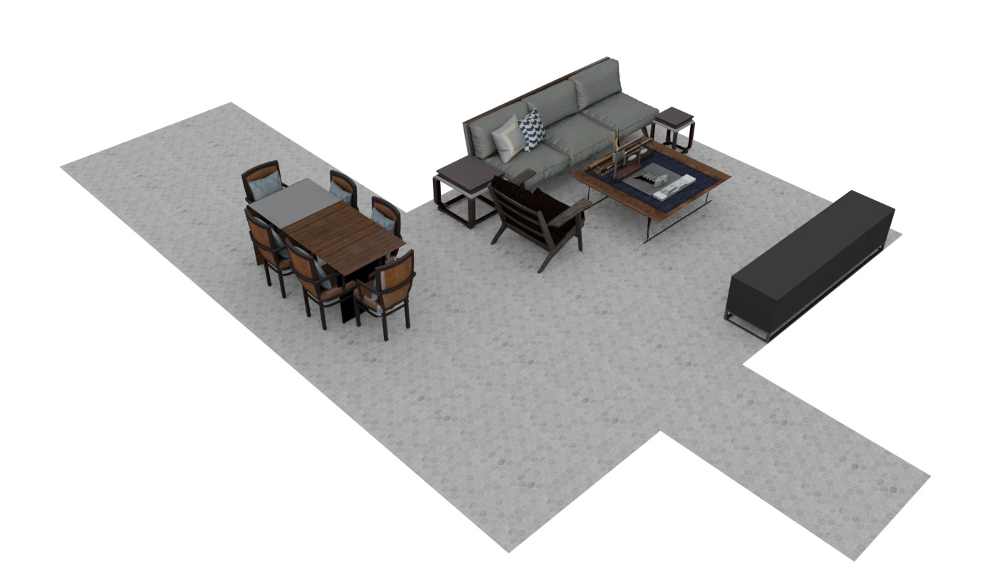
(a) Perspective view of the partial floorplan

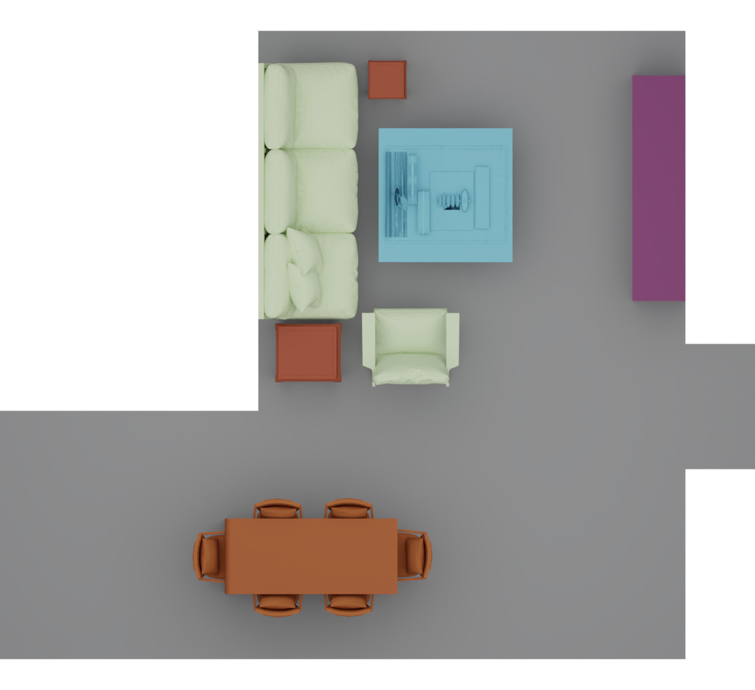
(b) Simplified Orthographic view

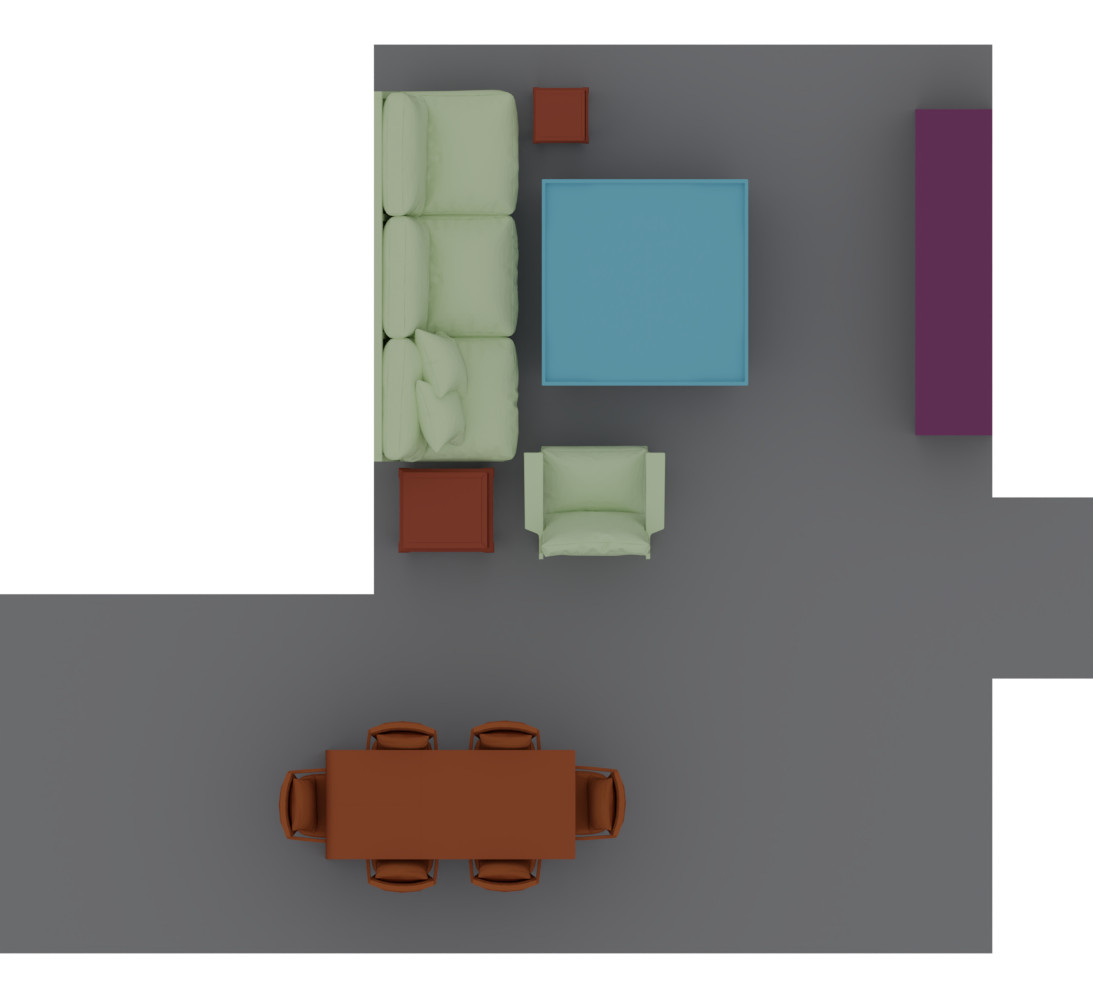
(c) Unconditionally sampled table (cyan).

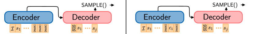
(d) Left: Unconditional Sampling Right: Conditioning by specifying attributes in $C$.

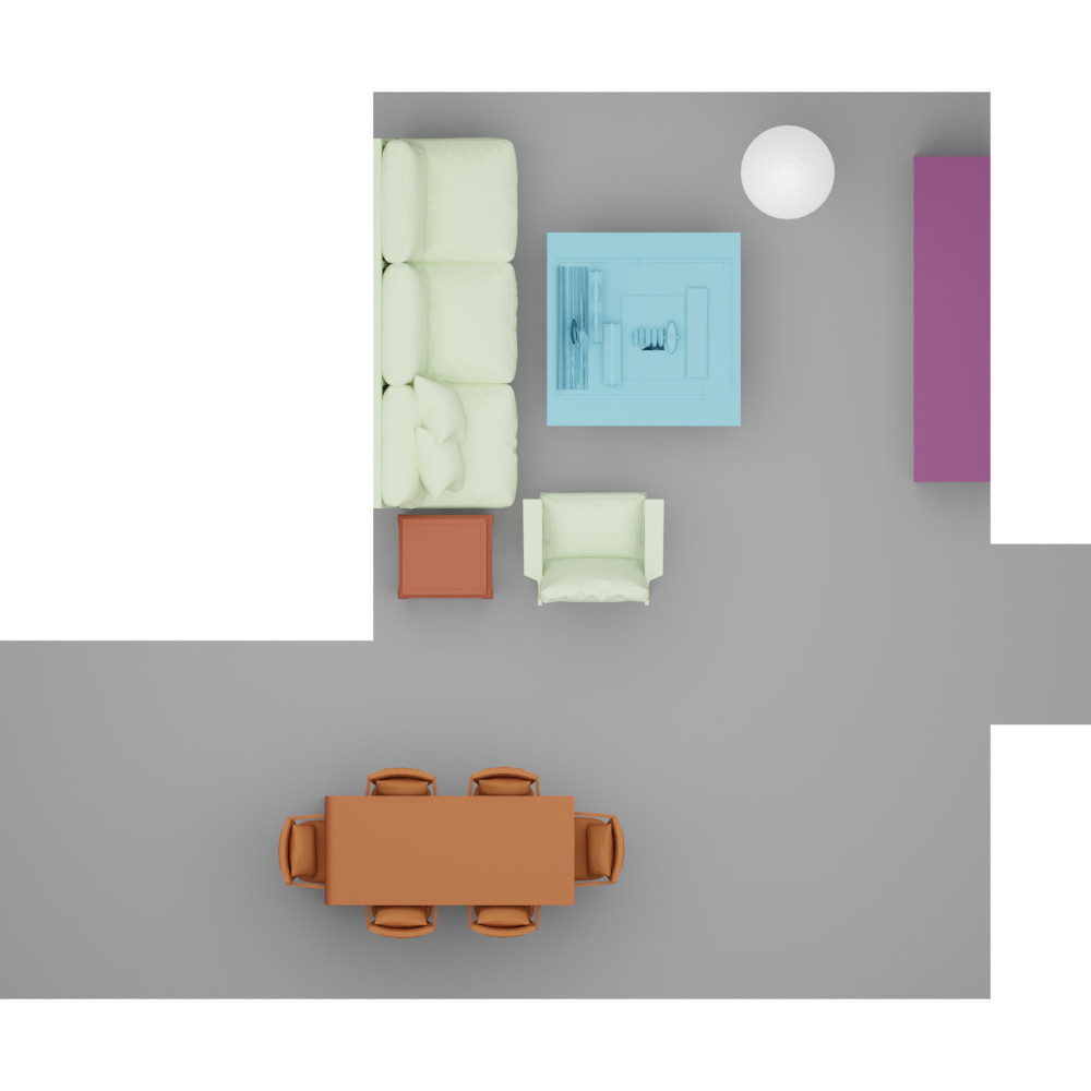
(e) We constrain the location of the object to be sampled. Shown by the white circle.

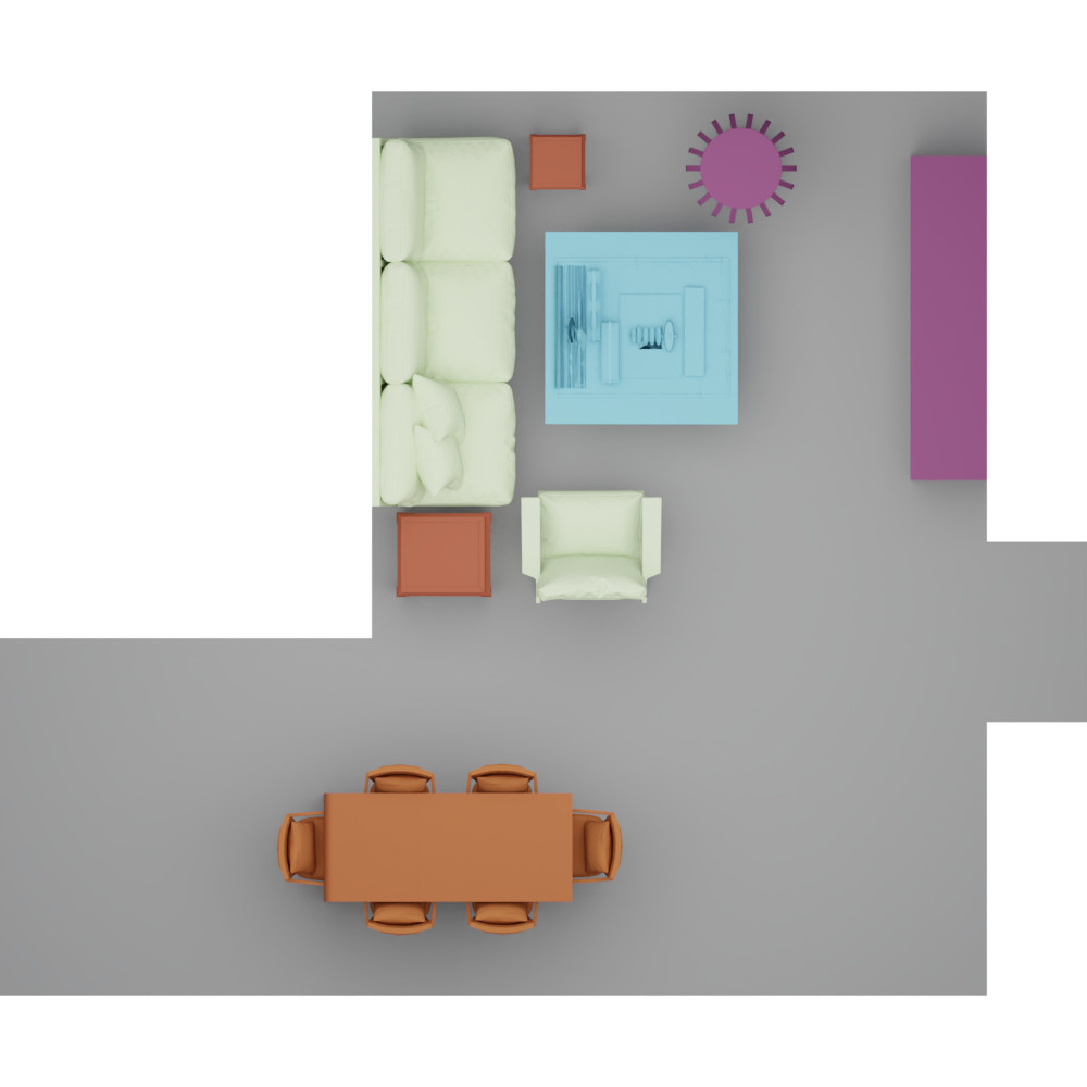
(f) Conditionally generated sample. (Purple)

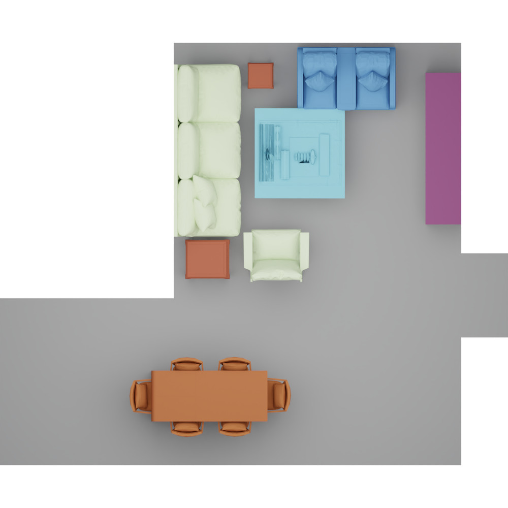
(g) We now condition the size to be large. The class automatically changes to satisfy the conditioning input.

(h) Ground-truth Floorplan

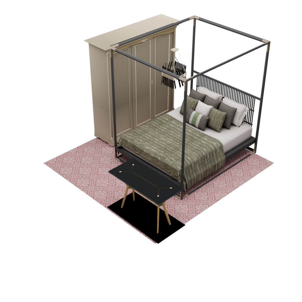
(i) We fill the class tokens in $C$ to correspond to lamp, bed, wardrobe, table.

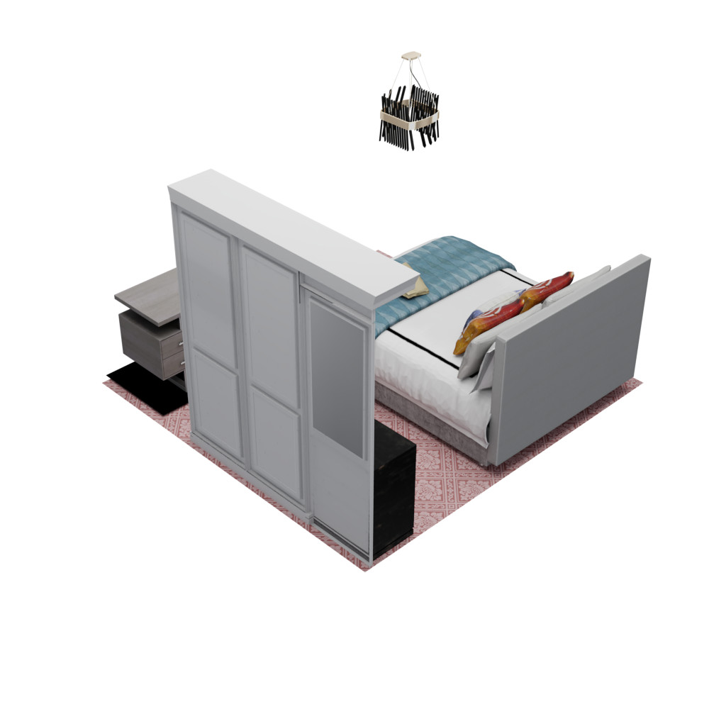
(j) Same conditioning as before, but now we constrain the angle of the bed.

(k) Ground-Truth Floorplan

(l) We condition to have two beds angled opposite each other, and two nightstands.

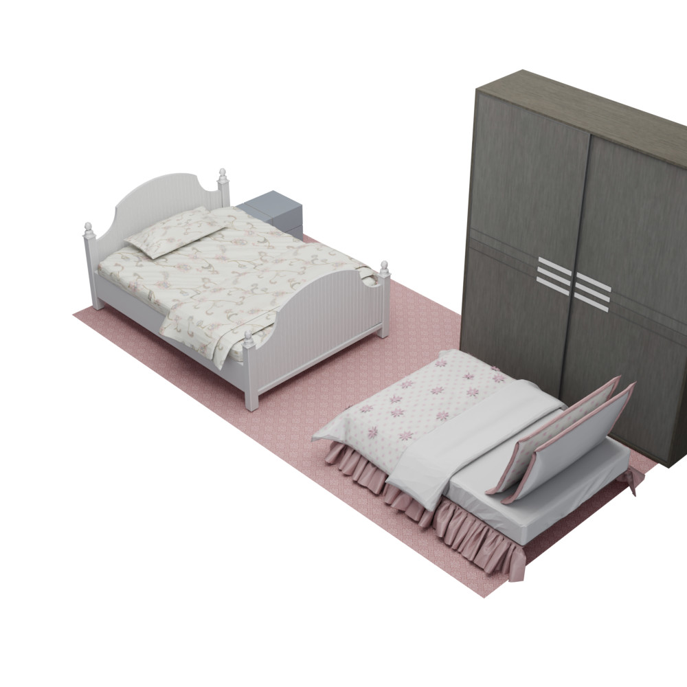
(m) We change one nightstand to be a wardrobe.

We show additional results on unconditional sampling from our model in the concluding figures. Our synthesised layouts are novel and do not merely copy the ground-truth layout. In addition, we see that our layouts respect the floorplan boundary and mimic the underlying style of the datasets, in terms of object-object co-occurrence.

Boundary

GT

ATISS

Ours

\begin{overpic}[width=433.62pt,clip]{figures/suppl/addl/lib/gt_Library-361_orthopng.jpg} \end{overpic}

\begin{overpic}[width=433.62pt,clip]{figures/suppl/addl/lib/atiss_Library-361_orthopng.jpg} \end{overpic}

\begin{overpic}[width=433.62pt,clip]{figures/suppl/addl/lib/ours_Library-361_orthopng.jpg} \end{overpic}

\begin{overpic}[width=433.62pt,clip]{figures/suppl/addl/lib/gt_Library-1511_orthopng.jpg} \end{overpic}

\begin{overpic}[width=433.62pt,clip]{figures/suppl/addl/lib/atiss_Library-1511_orthopng.jpg} \end{overpic}

\begin{overpic}[width=433.62pt,clip]{figures/suppl/addl/lib/ours_Library-1511_orthopng.jpg} \end{overpic}

\begin{overpic}[width=433.62pt,clip]{figures/suppl/addl/lib/gt_Library-20559_orthopng.jpg} \end{overpic}

\begin{overpic}[width=433.62pt,clip]{figures/suppl/addl/lib/atiss_Library-20559_orthopng.jpg} \end{overpic}

\begin{overpic}[width=433.62pt,clip]{figures/suppl/addl/lib/ours_Library-20559_orthopng.jpg} \end{overpic}

\begin{overpic}[width=433.62pt,clip]{figures/suppl/addl/lib/gt_Library-36052_orthopng.jpg} \end{overpic}

\begin{overpic}[width=433.62pt,clip]{figures/suppl/addl/lib/atiss_Library-36052_orthopng.jpg} \end{overpic}

\begin{overpic}[width=433.62pt,clip]{figures/suppl/addl/lib/ours_Library-36052_orthopng.jpg} \end{overpic}

\begin{overpic}[width=433.62pt,clip]{figures/suppl/addl/lib/gt_Library-38282_orthopng.jpg} \end{overpic}

\begin{overpic}[width=433.62pt,clip]{figures/suppl/addl/lib/atiss_Library-38282_orthopng.jpg} \end{overpic}

\begin{overpic}[width=433.62pt,clip]{figures/suppl/addl/lib/ours_Library-38282_orthopng.jpg} \end{overpic}

\begin{overpic}[width=433.62pt,clip]{figures/suppl/addl/lib/gt_Library-117651_orthopng.jpg} \end{overpic}

\begin{overpic}[width=433.62pt,clip]{figures/suppl/addl/lib/atiss_Library-117651_orthopng.jpg} \end{overpic}

\begin{overpic}[width=433.62pt,clip]{figures/suppl/addl/lib/ours_Library-117651_orthopng.jpg} \end{overpic}

Figure 11: Scene generation from scratch: We compare generated scenes from GT, ATISS, and our model on Library class.

Boundary

GT

ATISS

Ours

\begin{overpic}[width=433.62pt,clip]{figures/suppl/addl/bed/gt_SecondBedroom-9594_orthopng.jpg} \end{overpic}

\begin{overpic}[width=433.62pt,clip]{figures/suppl/addl/bed/atiss_SecondBedroom-9594_orthopng.jpg} \end{overpic}

\begin{overpic}[width=433.62pt,clip]{figures/suppl/addl/bed/SecondBedroom-9594_orthopng.jpg} \end{overpic}

\begin{overpic}[width=433.62pt,clip]{figures/suppl/addl/bed/gt_SecondBedroom-36408_orthopng.jpg} \end{overpic}

\begin{overpic}[width=433.62pt,clip]{figures/suppl/addl/bed/atiss_SecondBedroom-36408_orthopng.jpg} \end{overpic}

\begin{overpic}[width=433.62pt,clip]{figures/suppl/addl/bed/ours_SecondBedroom-36408_orthopng.jpg} \end{overpic}

\begin{overpic}[width=433.62pt,clip]{figures/suppl/addl/bed/gt_Bedroom-74674_orthopng.jpg} \end{overpic}

\begin{overpic}[width=433.62pt,clip]{figures/suppl/addl/bed/atiss_Bedroom-74674_orthopng.jpg} \end{overpic}

\begin{overpic}[width=433.62pt,clip]{figures/suppl/addl/bed/ours_Bedroom-74674_orthopng.jpg} \end{overpic}

\begin{overpic}[width=433.62pt,clip]{figures/suppl/addl/bed/gt_Bedroom-148896_orthopng.jpg} \end{overpic}

\begin{overpic}[width=433.62pt,clip]{figures/suppl/addl/bed/atiss_Bedroom-148896_orthopng.jpg} \end{overpic}

\begin{overpic}[width=433.62pt,clip]{figures/suppl/addl/bed/ours_Bedroom-148896_orthopng.jpg} \end{overpic}

\begin{overpic}[width=433.62pt,clip]{figures/suppl/addl/bed/gt_MasterBedroom-8979_orthopng.jpg} \end{overpic}

\begin{overpic}[width=433.62pt,clip]{figures/suppl/addl/bed/atiss_MasterBedroom-8979_orthopng.jpg} \end{overpic}

\begin{overpic}[width=433.62pt,clip]{figures/suppl/addl/bed/MasterBedroom-8979_orthopng.jpg} \end{overpic}

\begin{overpic}[width=433.62pt,clip]{figures/suppl/addl/bed/gt_MasterBedroom-27127_orthopng.jpg} \end{overpic}

\begin{overpic}[width=433.62pt,clip]{figures/suppl/addl/bed/atiss_MasterBedroom-27127_orthopng.jpg} \end{overpic}

\begin{overpic}[width=433.62pt,clip]{figures/suppl/addl/bed/ours_MasterBedroom-27127_orthopng.jpg} \end{overpic}

Figure 12: Scene generation from scratch: We compare generated scenes from GT, ATISS, and our model on Bedroom class.

Boundary

GT

ATISS

Ours

\begin{overpic}[width=346.89731pt,clip]{figures/suppl/addl/din/gt_LivingDiningRoom-1767_orthopng.jpg} \end{overpic}

\begin{overpic}[width=346.89731pt,clip]{figures/suppl/addl/din/464_atiss_fixed_orthopng.jpg} \end{overpic}

\begin{overpic}[width=346.89731pt,clip]{figures/suppl/addl/din/ours_LivingDiningRoom-1767_orthopng.jpg} \end{overpic}

\begin{overpic}[width=433.62pt,clip]{figures/suppl/addl/din/gt_LivingDiningRoom-4027_orthopng.jpg} \end{overpic}

\begin{overpic}[width=433.62pt,clip]{figures/suppl/addl/din/atiss_LivingDiningRoom-4027_orthopng.jpg} \end{overpic}

\begin{overpic}[width=433.62pt,clip]{figures/suppl/addl/din/LivingDiningRoom-4027_orthopng.jpg} \end{overpic}

\begin{overpic}[width=433.62pt,clip]{figures/suppl/addl/din/gt_LivingDiningRoom-9139_orthopng.jpg} \end{overpic}

\begin{overpic}[width=433.62pt,clip]{figures/suppl/addl/din/atiss_LivingDiningRoom-9139_orthopng.jpg} \end{overpic}

\begin{overpic}[width=433.62pt,clip]{figures/suppl/addl/din/LivingDiningRoom-9139_orthopng.jpg} \end{overpic}

\begin{overpic}[width=433.62pt,clip]{figures/suppl/addl/din/gt_LivingDiningRoom-18479_orthopng.jpg} \end{overpic}

\begin{overpic}[width=433.62pt,clip]{figures/suppl/addl/din/atiss_LivingDiningRoom-18479_orthopng.jpg} \end{overpic}

\begin{overpic}[width=433.62pt,clip]{figures/suppl/addl/din/LivingDiningRoom-18479_orthopng.jpg} \end{overpic}

\begin{overpic}[width=433.62pt,clip]{figures/suppl/addl/din/gt_LivingDiningRoom-25795_orthopng.jpg} \end{overpic}

\begin{overpic}[width=433.62pt,clip]{figures/suppl/addl/din/atiss_LivingDiningRoom-25795_orthopng.jpg} \end{overpic}

\begin{overpic}[width=433.62pt,clip]{figures/suppl/addl/din/LivingDiningRoom-25795_orthopng.jpg} \end{overpic}

\begin{overpic}[width=433.62pt,clip]{figures/suppl/addl/din/gt_LivingDiningRoom-81868_orthopng.jpg} \end{overpic}

\begin{overpic}[width=433.62pt,clip]{figures/suppl/addl/din/atiss_LivingDiningRoom-81868_orthopng.jpg} \end{overpic}

\begin{overpic}[width=433.62pt,clip]{figures/suppl/addl/din/ours_LivingDiningRoom-81868_orthopng.jpg} \end{overpic}

Figure 13: Scene generation from scratch: We compare generated scenes from GT, ATISS, and our model on Dining class.

Boundary

GT

ATISS

Ours

\begin{overpic}[width=346.89731pt,clip]{figures/suppl/addl/liv/gt_LivingDiningRoom-1806_orthopng.jpg} \end{overpic}

\begin{overpic}[width=346.89731pt,clip]{figures/suppl/addl/liv/atiss_LivingDiningRoom-1806_orthopng.jpg} \end{overpic}

\begin{overpic}[width=346.89731pt,clip]{figures/suppl/addl/liv/LivingDiningRoom-1806_orthopng.jpg} \end{overpic}

\begin{overpic}[width=433.62pt,clip]{figures/suppl/addl/liv/gt_LivingDiningRoom-4192_orthopng.jpg} \end{overpic}

\begin{overpic}[width=433.62pt,clip]{figures/suppl/addl/liv/atiss_LivingDiningRoom-4192_orthopng.jpg} \end{overpic}

\begin{overpic}[width=433.62pt,clip]{figures/suppl/addl/liv/LivingDiningRoom-4192_orthopng.jpg} \end{overpic}

\begin{overpic}[width=433.62pt,clip]{figures/suppl/addl/liv/gt_LivingDiningRoom-9921_orthopng.jpg} \end{overpic}

\begin{overpic}[width=433.62pt,clip]{figures/suppl/addl/liv/atiss_LivingDiningRoom-9921_orthopng.jpg} \end{overpic}

\begin{overpic}[width=433.62pt,clip]{figures/suppl/addl/liv/ours_LivingDiningRoom-9921_orthopng.jpg} \end{overpic}

\begin{overpic}[width=433.62pt,clip]{figures/suppl/addl/liv/gt_LivingDiningRoom-21284_orthopng.jpg} \end{overpic}

\begin{overpic}[width=433.62pt,clip]{figures/suppl/addl/liv/atiss_LivingRoom-111675_orthopng.jpg} \end{overpic}

\begin{overpic}[width=433.62pt,clip]{figures/suppl/addl/liv/LivingDiningRoom-21284_orthopng.jpg} \end{overpic}

\begin{overpic}[width=346.89731pt,clip]{figures/suppl/addl/liv/gt_LivingRoom-21557_orthopng.jpg} \end{overpic}

\begin{overpic}[width=346.89731pt,clip]{figures/suppl/addl/liv/atiss_LivingRoom-21557_orthopng.jpg} \end{overpic}

\begin{overpic}[width=346.89731pt,clip]{figures/suppl/addl/liv/ours_LivingRoom-21557_orthopng.jpg} \end{overpic}

\begin{overpic}[width=433.62pt,clip]{figures/suppl/addl/liv/gt_LivingRoom-111675_orthopng.jpg} \end{overpic}

\begin{overpic}[width=433.62pt,clip]{figures/suppl/addl/liv/253_living_atiss_fixed_orthopng.jpg} \end{overpic}

\begin{overpic}[width=433.62pt,clip]{figures/suppl/addl/liv/LivingRoom-111675_orthopng.jpg} \end{overpic}

Figure 14: Scene generation from scratch: We compare generated scenes from GT, ATISS, and our model on Living class.

Table 4: Summary of key notation used in the paper.

Symbol	Description
$\mathcal{I}$	A binary image representation of the floorplan boundary.
$g_{\phi}$	The Condition encoder. Implemented as Transformer Encoder with Bidirectional Attention.
$f_{\theta}$	The Generative Model. Implemented as Transformer Decoder with Causal Attention.
$g_{\psi}^{\mathcal{I}}$	The Boundary Encoder. An untrained ResNet-18 model.
$\mathcal{M}/\texttt{[MASK]}$	A learnable token representing a missing value which the Generative Model tries to predict.
$C$	The sequence of tokens describing the condition. It is the input to the Condition Encoder.
$c_{i}$	The $i$-th element of $C$.
$C^{g}$	The output of the last layer of the Condition Encoder. Encodes conditions from $C$ and boundary $\mathcal{I}$.
$S$	The sequence representing the layout.
$S^{GT}$	The sequence representation of the Ground Truth layout.
$s_{i}$	The $i$-th element of $S$.

References

- [1] Tom B. Brown, Benjamin Mann, Nick Ryder, Melanie Subbiah, Jared Kaplan, Prafulla Dhariwal, Arvind Neelakantan, Pranav Shyam, Girish Sastry, Amanda Askell, Sandhini Agarwal, Ariel Herbert-Voss, Gretchen Krueger, Tom Henighan, Rewon Child, Aditya Ramesh, Daniel M. Ziegler, Jeffrey Wu, Clemens Winter, Christopher Hesse, Mark Chen, Eric Sigler, Mateusz Litwin, Scott Gray, Benjamin Chess, Jack Clark, Christopher Berner, Sam McCandlish, Alec Radford, Ilya Sutskever, and Dario Amodei. Language models are few-shot learners. 2020.
- [2] Nicolas Carion, Francisco Massa, Gabriel Synnaeve, Nicolas Usunier, Alexander Kirillov, and Sergey Zagoruyko. End-to-end object detection with transformers. In ECCV, 2020.
- [3] Huiwen Chang, Han Zhang, Lu Jiang, Ce Liu, and William T. Freeman. Maskgit: Masked generative image transformer. In The IEEE Conference on Computer Vision and Pattern Recognition (CVPR), June 2022.
- [4] R. Qi Charles, Hao Su, Mo Kaichun, and Leonidas J. Guibas. Pointnet: Deep learning on point sets for 3d classification and segmentation. In 2017 IEEE Conference on Computer Vision and Pattern Recognition (CVPR), pages 77–85, 2017.
- [5] Shuai Li Chenhang He, Ruihuang Li and Lei Zhang. Voxel set transformer: A set-to-set approach to 3d object detection from point clouds. In Proceedings of the IEEE Conference on Computer Vision and Pattern Recognition, 2022.
- [6] Blender Online Community. Blender - a 3D modelling and rendering package. Blender Foundation, Stichting Blender Foundation, Amsterdam, 2018.
- [7] Jia Deng, Wei Dong, Richard Socher, Li-Jia Li, Kai Li, and Li Fei-Fei. Imagenet: A large-scale hierarchical image database. In 2009 IEEE conference on computer vision and pattern recognition, pages 248–255. Ieee, 2009.
- [8] Jacob Devlin, Ming-Wei Chang, Kenton Lee, and Kristina Toutanova. BERT: Pre-training of deep bidirectional transformers for language understanding. In Proceedings of the 2019 Conference of the North American Chapter of the Association for Computational Linguistics: Human Language Technologies, Volume 1 (Long and Short Papers), pages 4171–4186, Minneapolis, Minnesota, June 2019. Association for Computational Linguistics.
- [9] Patrick Esser, Robin Rombach, and Björn Ommer. Taming transformers for high-resolution image synthesis. In 2021 IEEE/CVF Conference on Computer Vision and Pattern Recognition (CVPR), pages 12868–12878, 2021.
- [10] Matthew Fisher, Daniel Ritchie, Manolis Savva, Thomas Funkhouser, and Pat Hanrahan. Example-based synthesis of 3d object arrangements. ACM Trans. Graph., 31(6), Nov 2012.
- [11] Huan Fu, Bowen Cai, Lin Gao, Ling-Xiao Zhang, Jiaming Wang, Cao Li, Qixun Zeng, Chengyue Sun, Rongfei Jia, Binqiang Zhao, and Hao Zhang. 3d-front: 3d furnished rooms with layouts and semantics. In 2021 IEEE/CVF International Conference on Computer Vision (ICCV), pages 10913–10922, 2021.
- [12] Kaiming He, Xiangyu Zhang, Shaoqing Ren, and Jian Sun. Deep residual learning for image recognition. In 2016 IEEE Conference on Computer Vision and Pattern Recognition (CVPR), pages 770–778, 2016.
- [13] Dan Hendrycks and Kevin Gimpel. Gaussian Error Linear Units (GELUs). arXiv e-prints, page arXiv:1606.08415, June 2016.
- [14] Thibaut Issenhuth, Ugo Tanielian, Jérémie Mary, and David Picard. Edibert, a generative model for image editing. arXiv preprint arXiv:2111.15264, 2021.
- [15] A. Katharopoulos, A. Vyas, N. Pappas, and F. Fleuret. Transformers are rnns: Fast autoregressive transformers with linear attention. In Proceedings of the International Conference on Machine Learning (ICML), 2020.
- [16] Diederik P. Kingma and Jimmy Ba. Adam: A method for stochastic optimization. In Yoshua Bengio and Yann LeCun, editors, 3rd International Conference on Learning Representations, ICLR 2015, San Diego, CA, USA, May 7-9, 2015, Conference Track Proceedings, 2015.
- [17] Alex Krizhevsky. One weird trick for parallelizing convolutional neural networks. CoRR, abs/1404.5997, 2014.
- [18] Juho Lee, Yoonho Lee, Jungtaek Kim, Adam Kosiorek, Seungjin Choi, and Yee Whye Teh. Set transformer: A framework for attention-based permutation-invariant neural networks. In Proceedings of the 36th International Conference on Machine Learning, pages 3744–3753, 2019.
- [19] Mike Lewis, Yinhan Liu, Naman Goyal, Marjan Ghazvininejad, Abdelrahman Mohamed, Omer Levy, Veselin Stoyanov, and Luke Zettlemoyer. BART: Denoising sequence-to-sequence pre-training for natural language generation, translation, and comprehension. In Proceedings of the 58th Annual Meeting of the Association for Computational Linguistics, pages 7871–7880, Online, July 2020. Association for Computational Linguistics.
- [20] Yinhan Liu, Myle Ott, Naman Goyal, Jingfei Du, Mandar Joshi, Danqi Chen, Omer Levy, Mike Lewis, Luke Zettlemoyer, and Veselin Stoyanov. Roberta: A robustly optimized bert pretraining approach. arXiv preprint arXiv:1907.11692, 2019.
- [21] Ilya Loshchilov and Frank Hutter. Decoupled weight decay regularization. In International Conference on Learning Representations, 2019.
- [22] Elman Mansimov, Alex Wang, and Kyunghyun Cho. A generalized framework of sequence generation with application to undirected sequence models, 2020.
- [23] Dror Moran, Hodaya Koslowsky, Yoni Kasten, Haggai Maron, Meirav Galun, and Ronen Basri. Deep permutation equivariant structure from motion. In 2021 IEEE/CVF International Conference on Computer Vision (ICCV), pages 5956–5966, 2021.
- [24] Wamiq Para, Paul Guerrero, Tom Kelly, Leonidas Guibas, and Peter Wonka. Generative layout modeling using constraint graphs. In 2021 IEEE/CVF International Conference on Computer Vision (ICCV), pages 6670–6680, 2021.
- [25] Gaurav Parmar, Richard Zhang, and Jun-Yan Zhu. On aliased resizing and surprising subtleties in gan evaluation. In CVPR, 2022.
- [26] Despoina Paschalidou, Amlan Kar, Maria Shugrina, Karsten Kreis, Andreas Geiger, and Sanja Fidler. Atiss: Autoregressive transformers for indoor scene synthesis. In Advances in Neural Information Processing Systems (NeurIPS), 2021.
- [27] Adam Paszke, Sam Gross, Francisco Massa, Adam Lerer, James Bradbury, Gregory Chanan, Trevor Killeen, Zeming Lin, Natalia Gimelshein, Luca Antiga, Alban Desmaison, Andreas Kopf, Edward Yang, Zachary DeVito, Martin Raison, Alykhan Tejani, Sasank Chilamkurthy, Benoit Steiner, Lu Fang, Junjie Bai, and Soumith Chintala. Pytorch: An imperative style, high-performance deep learning library. In Advances in Neural Information Processing Systems 32, pages 8024–8035. Curran Associates, Inc., 2019.
- [28] Alec Radford, Jeff Wu, Rewon Child, David Luan, Dario Amodei, and Ilya Sutskever. Language models are unsupervised multitask learners. 2019.
- [29] Siamak Ravanbakhsh, Jeff Schneider, and Barnabas Poczos. Deep learning with sets and point clouds. arXiv preprint arXiv:1611.04500, 2016.
- [30] Daniel Ritchie, Kai Wang, and Yu-An Lin. Fast and flexible indoor scene synthesis via deep convolutional generative models. In 2019 IEEE/CVF Conference on Computer Vision and Pattern Recognition (CVPR), pages 6175–6183, 2019.
- [31] Julian Salazar, Davis Liang, Toan Q. Nguyen, and Katrin Kirchhoff. Masked language model scoring. In Proceedings of the 58th Annual Meeting of the Association for Computational Linguistics, pages 2699–2712, Online, July 2020. Association for Computational Linguistics.
- [32] Tim Salimans, Andrej Karpathy, Xi Chen, and Diederik P. Kingma. Pixelcnn++: A pixelcnn implementation with discretized logistic mixture likelihood and other modifications. In ICLR, 2017.
- [33] Nicolas Ugrinovic, Adria Ruiz, Antonio Agudo, Alberto Sanfeliu, and Francesc Moreno-Noguer. Permutation-invariant relational network for multi-person 3d pose estimation. arXiv preprint arXiv:2204.04913, 2022.
- [34] Ashish Vaswani, Noam Shazeer, Niki Parmar, Jakob Uszkoreit, Llion Jones, Aidan N. Gomez, Łukasz Kaiser, and Illia Polosukhin. Attention is all you need. In Proceedings of the 31st International Conference on Neural Information Processing Systems, NIPS’17, page 6000–6010, Red Hook, NY, USA, 2017. Curran Associates Inc.
- [35] Alex Wang and Kyunghyun Cho. Bert has a mouth, and it must speak: Bert as a markov random field language model. arXiv preprint arXiv:1902.04094, 2019.
- [36] Kai Wang, Yu-An Lin, Ben Weissmann, Manolis Savva, Angel X. Chang, and Daniel Ritchie. Planit: Planning and instantiating indoor scenes with relation graph and spatial prior networks. ACM Trans. Graph., 38(4), jul 2019.
- [37] Xinpeng Wang, Chandan Yeshwanth, and Matthias Nießner. Sceneformer: Indoor scene generation with transformers. In 2021 International Conference on 3D Vision (3DV), pages 106–115. IEEE, 2021.
- [38] Tomer Weiss, Alan Litteneker, Noah Duncan, Masaki Nakada, Chenfanfu Jiang, Lap-Fai Yu, and Demetri Terzopoulos. Fast and scalable position-based layout synthesis. IEEE Transactions on Visualization and Computer Graphics, 25(12):3231–3243, 2019.
- [39] Lap-Fai Yu, Sai-Kit Yeung, Chi-Keung Tang, Demetri Terzopoulos, Tony F. Chan, and Stanley J. Osher. Make it home: Automatic optimization of furniture arrangement. ACM Trans. Graph., 30(4), Jul 2011.
- [40] Manzil Zaheer, Satwik Kottur, Siamak Ravanbakhsh, Barnabas Poczos, Ruslan R Salakhutdinov, and Alexander J Smola. Deep sets. In I. Guyon, U. V. Luxburg, S. Bengio, H. Wallach, R. Fergus, S. Vishwanathan, and R. Garnett, editors, Advances in Neural Information Processing Systems 30, pages 3391–3401. Curran Associates, Inc., 2017.