Polarimetric characterization of segmented mirrors

Abstract

We study the impact of the loss of axial symmetry around the optical axis on the polarimetric properties of a telescope with segmented primary mirror when each segment is present in a different aging stage. The different oxidation stage of each segment as they are substituted in time leads to non-negligible cross-talk terms. This effect is wavelength dependent and it is mainly determined by the properties of the reflecting material. For an aluminum coating, the worst polarimetric behavior due to oxidation is found for the blue part of the visible. Contrarily, dust —as modeled in this work— does not significantly change the polarimetric behavior of the optical system . Depending on the telescope, there might be segment substitution sequences that strongly attenuate this instrumental polarization.

1 Introduction

The new generation of large telescopes, such as the European Extremely Large Telescope (E-ELT) [1] or the Thirty Meter Telescope (TMT)[2] plan gigantic and segmented primary surfaces. As an example, the collecting area of the E-ELT primary mirror is larger than a basketball court. Maintaining the homogeneity of such a huge optical surface is a big challenge —perhaps an impossible one—. Removing, aluminizing and installing each of its 798 hexagonal segments may take over a year and by then, there will be a significant degradation on the first ones. One consequence of an inhomogeneous primary mirror is simply a reduced reflectivity. Another potentially more critical effect might be its impact on polarization and the polarimetric properties of the telescope. Polarization is of special relevance from a diagnostic point of view because it is intimately related with any symmetry breaking phenomenon taking place on the object of interest or the presence of magnetic fields. Thus it is possible to study, among others, the magnetic dynamo in the Sun and other cool stars [3], the spatial geometry of (either magnetic or non-magnetic) physical systems such as planetary nebulae [4], even spatially unresolved stars opening up the possibility of carrying out stellar imaging [5], the study of active galactic nuclei [6] or the presence and properties of extra-solar planets [7], with specific geometrical configurations that give rise to specific polarization states. Finally, there is increasing bibliography on the potential applicability of the polarization of the light in order to find extraterrestrial life [8].

Oblique reflection in an optical surface polarizes (linearly, perpendicularly to the plane of reflection) the incoming light [9]. Most telescopes have primary and secondary mirrors in an axially symmetric configuration. Their net instrumental polarization (along the optical axis) is zero because two points in the mirror located at the same distance from the optical axis but $90^{\circ}$ apart should polarize to the same degree but with opposite sign. In fact, this property can be used on the whole optical path to design telescopes that are free of instrumental polarization, such as the European Solar Telescope (EST)[10]. Large 10-meter class telescopes with segmented hexagonal mirrors are not axially symmetric but the 6-fold symmetry of their mirrors should also lead to perfect cancellation after integration over the whole mirror.

Also, in smaller telescopes, the angles of incidence are very close to normal which severely limits the amount of instrumental polarization generated by the primary and secondary mirrors. Reflections on the external parts of the primary mirror of the E-ELT can reach angles $\sim 15^{\circ}$ which may yield non-negligible polarization effects.

In addition, in telescopes with segmented primary mirrors, the maintenance of these elements is usually done in a sequential manner so that the scientific availability of the facility is maximized. Thus this process can introduce an additional source of symmetry loss in the optical system. Polarimetry in telescopes with segmented mirrors is already feasible (for instance CanariCam [11]) and will be more frequent soon as the incoming new generation instrumentation for the Gran Telescopio Canarias (GTC) —MIRADAS [12]— as well as part of the instrumentation to be installed in the future E-ELT are planning to acquire high sensitivity polarimetric data. It is thus of interest to evaluate the potential instrumental polarization that symmetry loss due to sequential segment substitution might introduce.

In this note we study the severity of the intrinsic inhomogeneity of the primary mirror in large segmented telescopes in general and in two cases of practical interest in particular —E-ELT and GTC—, with very different segment-to-mirror area ratios. In contrast to previous works [13, 14, 15], here we consider variations on the reflectivity of the segments due to oxidation of the aluminum (Al) and dust deposition characterizing the instrumental polarization of the primary and secondary mirrors. This study is valuable to understand the contribution to the global budget of instrumental polarization of the telescope, to design polarimetric calibration strategies to compensate for it, and to propose the most convenient segment replacement method to mitigate adverse effects.

2 Method

In this work we have developed a ray-tracing numerical code that evaluates the polarimetric properties of the segmented primary and secondary mirrors of two different telescopes: GTC and E-ELT, as we assume that we are dealing with plane waves (for more complex processes a more suitable formalism [16] could be employed). In particular, we investigate the effect on the polarimetric properties of the optical system as the axial symmetry with respect to the optical axis is broken either by the shape of the mirror itself or additional sources that might contribute to the loss of axial symmetry. To do so, we use the Stokes formalism, which allows to fully characterize the polarimetric properties of an optical system.

2.1 Reflecting surfaces

Figure 1: Elements of the primary reflecting surface: dust, aluminum oxide, aluminum, and Zerodur for a given segment at a timestep $t$.

In the Stokes formalism, the action of optical devices is described by linear transformations over the Stokes pseudo-vector, i.e. by means of $4\times 4$ matrices. The reflection on a mirror in this formalism is given by the following transformation matrix [17]:

$$\mathfrak{M}=\frac{1}{2}\left(\begin{array}[]{cccc}t_{1}&t_{2}&0&0\\ t_{2}&t_{1}&0&0\\ 0&0&t_{3}\cos\delta&t_{3}\sin\delta\\ 0&0&-t_{3}\sin\delta&t_{3}\cos\delta\end{array}\right),$$ (1)

where $t_{1}=|\rho^{\parallel}|^{2}+|\rho^{\perp}|^{2}$, $t_{2}=|\rho^{\parallel}|^{2}-|\rho^{\perp}|^{2}$, $t_{3}=2\rho^{\parallel}\rho^{\perp}$, and $\delta=\phi^{\perp}-\phi^{\parallel}$. The symbols $\rho$ and $\phi$ refer to the modulus and phase, respectively, of the Fresnel coefficients for reflection $r^{\parallel}$ and $r^{\perp}$:

$$r^{\parallel}=\rho^{\parallel}e^{i\phi^{\parallel}}$$ (2)

$$r^{\perp}=\rho^{\perp}e^{i\phi^{\perp}}.$$ (3)

The expressions of the Fresnel coefficients depend upon the specific composition of the surface in which light is reflected. For the primary mirror, the reflecting surface consists of the substrate of the mirror, the conductor, which is deposited above it, the oxide that forms above the conductor due to the action of the atmosphere and the dust that accumulates on top (Fig. 1). Except for dust, which we account for in a different way, the first three layers can be safely modeled by means of the thin film theory. According to this theory, the Fresnel coefficients do only depend on the thickness and the refractive indices (real or complex) of the films that form the reflective surface. We use the following formula [17] for their computation:

$$r^{\parallel}=\frac{(m_{11}+m_{12}\,p_{4})p_{1}-(m_{21}+m_{22}\,p_{4})}{(m_{11}+m_{12}\,p_{4})p_{1}+(m_{21}+m_{22}\,p_{4})},$$ (4)

where $p_{\rm k}=n_{\rm k}\cos\theta_{\rm k}$, with $k=1$ for air, $k=2$ for the oxide film, $k=3$ for the conductor and $k=4$ for the substrate. A similar expression is obtained for the perpendicular Fresnel coefficient ($r^{\perp}$) by using $q_{\rm k}=\frac{\cos\theta_{\rm k}}{n_{\rm k}}$ instead of $p_{\rm k}$ in Eq. (4). Eq. (4) has explicit dependence on both the air and substrate, while the intermediate layers enter through the characteristic matrix of the reflecting surface. The coefficients $m_{lm}$ of this matrix are given by:

$$M=\prod_{k=4}^{1}M_{\rm k}=\left(\begin{array}[]{cc}m_{11}&m_{12}\\ m_{21}&m_{22}\end{array}\right).$$ (5)

Each one of the characteristic matrices is given by the expression:

$$M_{\rm k}=\left(\begin{array}[]{cc}\cos\beta_{\rm k}&-\frac{i}{p_{\rm k}}\sin\beta_{\rm k}\\ -i\,p_{\rm k}\sin\beta_{\rm k}&\cos\beta_{\rm k}\end{array}\right),$$ (6)

where $\beta_{\rm k}=k_{0}\,n_{\rm k}\,d_{\rm k}\,\cos\theta_{\rm k}$, with $k_{0}$ being the wavenumber of the radiation, $n_{\rm k}$ being the refraction index of the $k$-th layer (either real or complex), $d_{\rm k}$ the thickness of the $k$-th layer and $\theta_{\rm k}$ the angle of incidence on the $k$-th layer.

The dust layer cannot be treated within the thin film formalism because the sizes of typical dust particles are already of the order of the wavelength of the light under consideration (typically in the visible or near infrared). The model that we choose is discussed in Sect. 2.5.

In order to simplify the interpretation of the results, we consider a secondary mirror made of a substrate layer over which we lay a conductor. No dust is considered since its deposition is less probable than on the primary mirror. Additionally, we keep the thickness of the conductor constant. Therefore, any variation of the polarization properties of the telescope is then associated with changes in the primary mirror.

With the previous theory, once the wavelength of the incoming radiation, the incidence angle and the thickness and reflecting indices of the various films are given, the calculation of the Fresnel coefficients for any reflection in the optical system is possible. This allows us to calculate the reflective properties for any incident ray of the system.

2.2 Geometrical setup

Table 1: Radius of curvature $R$ and conic constant $K$ for primary (^prim) and secondary (^sec) mirror of GTC and E-ELT considered. $d$ is the distance between the primary and secondary mirrors at the optical axis.

Parameter	GTC	E-ELT	Units
$R_{c}^{\rm prim}$	33.0	69.168	m
$K^{\rm prim}$	-1.002250	-0.993295	-
$R_{c}^{\rm sec}$	3.899678	9.313	m
$K^{\rm sec}$	-1.504835	-2.28962	-
$d$	14.73941	31.415	m

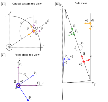
Figure 2: Panel a) shows the polarization reference system ($\hat{\rm e}^{0}$, in purple color) that has to be rotated by $\alpha_{1}$, which depends upon the $x$ and $y$ position of the ray, in order to get the reference system ($\hat{\rm e}^{1}$ in orange) so that reflection can be written as in Eq. (1). After that first rotation, there are two reflections and one additional rotation ($\alpha_{2}$) that take in the same fashion once in the $\hat{\rm a}-\hat{\rm z}$ plane, as depicted in panel b). Finally, panel c) shows the last rotation ($\alpha_{3}$) required in order to set the polarimetric properties of each point of the optical system in a common reference system ($\hat{\rm e}^{5}\equiv\hat{\rm e}^{0}$).

In order to know the angle of incidence needed for the calculation of $\beta_{\rm k}$ in Eq. (6) for both the primary and secondary mirrors, we need to know the inclination of the ray of light entering the telescope with respect to the optical axis. This parameter is an input supplied by the user, and in this work it will always be aligned with the optical axis of the system. For the numerical calculation, we consider many incoming light beams that reach the primary mirror in various positions. Panel a) of Fig. 2 shows (from a top view of the telescope) one potential case of such an incident ray. The reference system for the optical components is chosen so that $z$ is along the optical axis of the system and $x$ and $y$ in the plane perpendicular to it. $z=0$ is in the intersection of the optical axis with the surface described by the primary mirror (see for instance the side view of the system in panel b) of Fig. 2). To fully take into account the symmetry of the problem, the $(x,y)$ coordinates for the rays are defined following a quadrature in polar coordinates so that we ensure that every ray has its complementary one (i.e. at exactly the same distance but at 90^∘) if it is possible. An example of a very coarse quadrature for GTC is shown in panel b) of Fig. 3. In the figure, for each of the area elements (highlighted in magenta), we assume that the polarimetric properties are the ones given for the central point of that small area. Note here that, for the sake of clarity, this example shows the case for 240 rays, a very small number of rays. We also show all quadrature points, independently of whether they reach the focal plane of the telescope. Some of these rays will not reflect on the primary or on the secondary mirror, so they are excluded in the calculation.

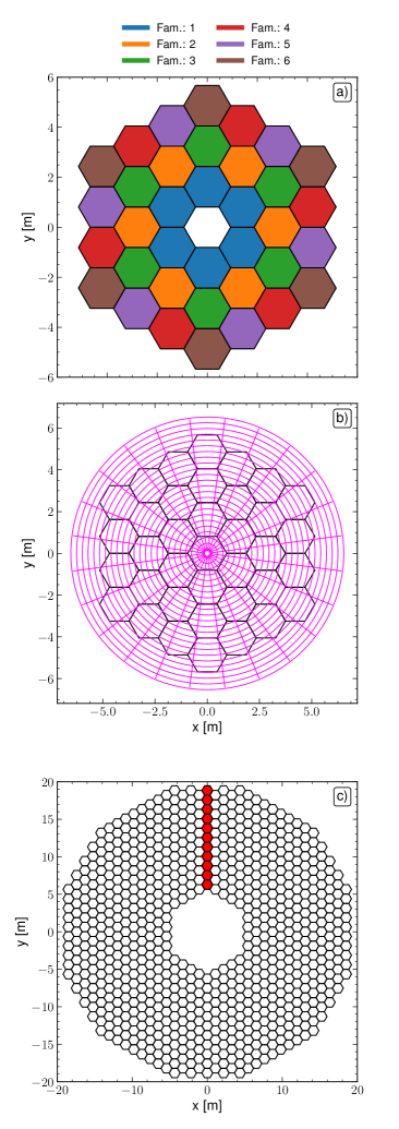
Figure 3: a) GTC primary mirror layout color coded according to the family of segments they belong to. b) Ray quadrature layout over GTC’s primary mirror layout. c) E-ELT’s primary mirror layout with the segments used in Fig. 6 highlighted in red.

In addition to the incident position of each ray, the calculation of the angle of incidence requires the knowledge of the specific shape of the primary mirror. For the telescopes here considered, the primary mirror is formed by gathering hexagonal segments (as seen from the optical axis). In Fig. 3 we show the segment distribution for each telescope: in panel a) for GTC in colored format and in panel c) for E-ELT. These are built following the specifications in the conceptual design for GTC (defined on 1997) and the construction proposal for the E-ELT (defined on 2011). They contain 36 and 798 hexagonal segments for the primary mirror, respectively. The segment side side size is 936 mm and 725 mm, respectively. A certain amount of hexagons are not present in the center so that each mirror keeps an approximate internal circular area with a radius of 0.4 and 4.7 m for GTC and E-ELT, respectively. The E-ELT secondary mirror is of circular shape and has a radius of 4.2 m. The secondary mirror of GTC is serrated with a maximum radius of 1.1766 m and an internal free area of hexagonal shape with a side size of 0.1388 m. In addition to the shape of the mirrors, we also need their curvature which, for the primary, is given by:

$$x^{2}+y^{2}-2\,R\,z+(1+K)\,z^{2}=0,$$ (7)

where the values for $R$ and $K$ are in Table 1 for both telescopes. Combining all these parameters one can determine the angle of incidence of each ray over the primary mirror. Once this reflection takes place, the light is reflected to the secondary mirror whose shape is given by:

$$x^{2}+y^{2}-2\,R\,\zeta+(1+K)\,\zeta^{2}=0,\\$$ (8)

with $\zeta=z-d$, being $d$ the distance between both mirrors along the optical axis. The actual values for the conic constant and the radius of curvature of the secondary mirror are also shown in Table 1.

With this information we can compute the angle of incidence for each ray both in the primary and secondary mirrors. Thus, in order to calculate the reflection matrices described in Sect. 2.1 we need the thickness and refractive indexes of each layer considered.

2.3 Thickness and refractive index

The aging of the various primary mirror segments requires taking into account the time variation of the conductor and oxide films thickness. As mentioned before the dust layer is handled differently and discussed in Sect. 2.5. Concerning the oxide thickness, we assume an exponential growth law. This is expected since at the beginning the conductor is directly exposed to air and so the oxidation is fast. Once the oxide film gets thicker, this oxide layer itself prevents the conductor from the contact with air and, consequently, the growth rate of the oxide film is strongly reduced. This way, the thickness of the oxide layer with time is assumed to be given by:

$$d_{2}=d_{\mathrm{ox}}^{\mathrm{max}}\,(1-e^{-t/\tau_{\rm ox}}),$$ (9)

where $d_{\mathrm{ox}}^{\mathrm{max}}$ is the maximum thickness allowed for the oxide layer, set here to 0.1 $\mu$m, $\tau_{\rm ox}$ is the growth rate for the oxide film, that we choose to be 1349 days, and $t$ is the time, measured in days, since the segment exchange. This behavior is complementary to that of the conductor (namely $d_{3}=d_{\mathrm{al}}^{0}-d_{2}$), for which we require an initial thickness: $d_{\mathrm{al}}^{0}=1$ $\mu$m.

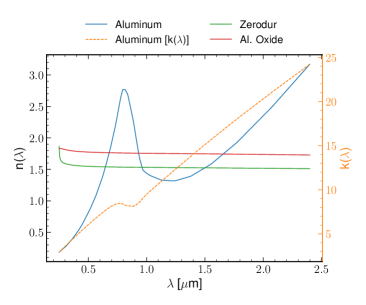
Figure 4: Refractive index’s real part (solid line) and imaginary part (dashed line) for the materials employed and their wavelength dependence.

In addition to the thickness of each layer, the calculation of the Mueller matrix requires the refractive index of each material, together with the wavelength variation (shown in Fig. 4). In this work, we assume that all mirrors are covered with aluminum (whose refractive index is complex), the oxide film is then aluminum oxide ($\text{Al}_{2}\text{O}_{3}$), the substrate is Zerodur.

2.4 Mueller matrix for each segment

With this modeling, it is possible to calculate the reflection matrix for each ray in both the primary and secondary mirrors. To do so, we have to take into account that the Mueller matrix for reflection as shown in Eq. (1) is only valid when the vector $\hat{e}_{\parallel}$ lies in the incidence-reflection plane. Since this is not the case in general, one has to include some additional rotations, which vary from ray to ray. These rotations ensure that the necessary conditions for validity of the reflection matrix are satisfied. The train of rotation is as follows: i) a first rotation ($\alpha_{1}$) transforms the system from the global reference frame for the Stokes parameters ($\hat{\rm e}^{0}$) to the one preferred for computing the reflection in each point of the primary mirror ($\hat{\rm e}^{1}$ see panel a) in Fig. 2), ii) a second rotation ($\alpha_{2}$) takes the outgoing reference frame from the first reflection ($\hat{\rm e}^{2}$) to the preferred one for the second reflection ($\hat{\rm e}^{3}$, panel b) in the figure), and iii) a third rotation ($\alpha_{3}$) takes the reference frame from the second reflection ($\hat{\rm e}^{4}$) back to the global reference frame ($\hat{\rm e}^{5}$ in panel c) of the figure). Thus, for each ray, the equivalent Mueller matrix of the two-mirror model here considered is given by:

$$\mathfrak{M}_{x,y}=R_{x,y}(\alpha_{3})\,\mathfrak{M}_{\rm x,y}^{\rm sec}\,R_{x,y}(\alpha_{2})\,\mathfrak{M}_{x,y}^{\rm prim}\,R_{\rm x,y}(\alpha_{1}),$$ (10)

where $R_{\rm x,y}(\alpha_{1}=\pi/2+\arctan(y/x))$ is the first rotation matrix for the point $x,y$ on the primary mirror (see panel a in Fig. 2), $\mathfrak{M}_{\rm x,y}^{\rm prim}$ is the reflection matrix for that point in the primary mirror, $R_{x,y}(\alpha_{2}=\pi)$ is the second rotation that takes the reference frame from that for the primary to the one needed for the secondary reflection, $\mathfrak{M}_{\rm x,y}^{\rm sec}$ takes into account the reflection on the secondary mirror, and $R_{\rm x,y}(\alpha_{3}=\pi/2-\arctan(y/x)=\pi-\alpha_{1})$ finally rotates to the common reference frame for polarization.

2.5 Dust

The last element to take into account is dust deposition on the mirrors as well as its modeling. We cannot use the thin-film theory because the typical size of a dust particle is already similar or larger than the wavelength for visible or near infrared light. In this work we model the effect of dust from a statistical point of view rather than individually for each ray beam. We assume that each segment is partly covered by dust. If a ray falls into a dusty area, then, by hypothesis that ray becomes part of stray light and disappears from the calculation. This is represented in Fig. 1 by a time-varying dust particle coverage. Mathematically, we propose that the incident light of each segment is modified by:

$$\mathfrak{M}_{\rm dust}^{i}=(1-p^{i}_{0}(t))1\!\!1,$$ (11)

where $1\!\!1$ is the identity matrix and $p^{i}_{0}$ is the probability of the incoming light hitting dust particles and thus disappearing. This parameter is segment-dependent in the sense that for a given time, each segment will be characterized by a different value of $p_{0}$, which is function of the time from the last segment exchange.

This way the effect of dust over each segment is described as a linear transformation whose action precedes to any other optical transformation , i.e. effectively it attenuates the incoming light reaching to each segment:

$$\mathfrak{M}^{\mathrm{final}}_{x,y}=\mathfrak{M}_{x,y}\mathfrak{M}_{\rm dust}^{i}$$ (12)

This is a very simplified approach for the effect of dust over an optical system but it includes the potential effect over polarization due to symmetry breaking effects produced by different amounts of dust in each segment. A more realistic model for dust deposition and its effect over the overall transmission of the system is out of the scope of this work.

2.6 Replacement sequences

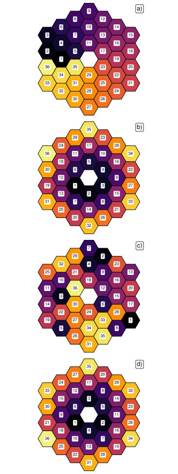
Figure 5: Segment substitution sequences for GTC: “azimuth” (panel a), “linear” (panel b), “random” (panel c), and “symmetry” (panel d). The label in each segment represents the position in the segment substitution sequence.

With the model described above we can fully characterize the polarimetric properties of any telescope (GTC and E-ELT in our case) for any given time. In order to study the effect that differential aging of each segment has over the polarimetric properties of the optical system, we consider different segment substitution strategies. Each substitution sequence will take place along a whole year (approximately), mimicking the substitution cadence that is already at work at GTC and the one expected for E-ELT. In the first substitution method, which is labeled as “azimuth” (see index labelling in panel a in Fig. 5 for the specific order for the case of GTC), we exchange the segments according to their azimuth value (and for segments with the same azimuth position, on the basis of their distance to the optical axis from the furthest to the closest). In the second case, labeled as “linear” (see panel b in Fig. 5), we exchange the segments according to their distance to the optical axis and, for these at same distance to the optical axis, according to their azimuth value. For the third case, labeled as “random” (see panel c in Fig. 5), we follow a random order exchanging the segments. The fourth case is labeled “symmetry” (see panel d in Fig. 5), where the segments are exchanged according to their distance to the optical axis and, for these at same distance to the optical axis, the segments are exchanged in such a way that two consecutive exchanges are done with a difference in the azimuth of the segments of 120^∘ or more.

Note that some of the sequences considered here are not actually feasible in practice. It is so because the designs for GTC and E-ELT mentioned above require a number of segments that share exactly the same shape, i.e. they are interchangeable. Segments that share the same shape are referred here as belonging to the same “family”. Consequently, in order to replace a segment and not leave a hole in the primary mirror it is mandatory to have an additional segment for each of these families. The number of families is 6 for GTC (see coloring in panel a of Fig. 3) and 133 for E-ELT. The planned cleaning strategy for E-ELT requires that two segments are changed daily, so that the sequences labeled “linear” and “symmetry” cannot be executed in practice, as it would require to have at least two additional segments per family instead of the only one planned. For GTC, any of the considered cases is applicable, as the cleaning process of each segment takes less than two days and segments are assumed to be changed every ten days. Also, the “random” sequence requires additional constraints because two mirrors of the same family cannot be exchanged in consecutive timesteps. Despite this limitation for E-ELT, we keep the analysis for all the substitution sequences considered for both telescopes to better visualize the importance of taking into account the differential aging of segments when doing polarimetry with segmented primary mirrors.

3 Results and discussion

We apply the polarimetric model with progressive complexity to the primary and secondary mirror trying to identify the contribution the different model parameters have on the polarimetric properties of the optical system.

3.1 Ideal reflection: individual segments

Figure 6: Mueller matrix for the eleven E-ELT segments highlighted in Fig. 3 as a function of their distance to the optical axis at 500 nm. Note that elements other than $\mathfrak{m}_{1,1}$ represent the reflection corrected value, i.e. $\tilde{\mathfrak{m}}_{i,j}=\mathfrak{m}_{i,j}/\mathfrak{m}_{1,1}$, for each distance value.

Before proceeding to the polarimetric characterization of the optical system as a whole, i.e. the integration over the whole surface area, it is worth considering the polarimetric properties of individual segments as they allow a more detailed insight into the system behavior. To do so, we consider the various E-ELT segments highlighted in red in Fig. 3. Figure 6 shows each Mueller matrix element value for these segments as a function of the distance to the optical axis. That is the only difference between the segments as here we are limiting ourselves to an ideal reflector, i.e., neither dust nor oxidation is considered. Due to the specific distribution of the segments (along the vertical direction) only elements $\tilde{\mathfrak{m}}_{2,1}$, $\tilde{\mathfrak{m}}_{1,2}$, $\tilde{\mathfrak{m}}_{4,3}$ , and $\tilde{\mathfrak{m}}_{3,4}$ take non-negligible values (apart from diagonal elements) as the segments are aligned with one of the polarization reference system. Note that, in Fig. 6, elements other than $\mathfrak{m}_{1,1}$ represent the reflection corrected value, i.e. $\tilde{\mathfrak{m}}_{i,j}=\mathfrak{m}_{i,j}/\mathfrak{m}_{1,1}$. The absolute amplitude of these Mueller elements increase as the segment distance to the optical axis increases. Thus, the same reflecting surface of a segment at two different distances from the optical will have a different impact on the polarimetric behavior of the whole telescope.

3.2 Ideal reflection: whole telescope

Now we consider the polarimetric properties of the whole optical system in the same ideal configuration, i.e. without dust or oxidation. In order to check this, we first look at the Mueller matrix for an ideal GTC using approximately $1.7\times 10^{7}$ rays at 500 nm:

$$\mathfrak{M}_{\rm GTC}^{\rm ideal}=\left(\begin{array}[]{cccc}0.844026&1^{-18}&1^{-19}&1^{-35}\\ 1^{-18}&0.844020&1^{-17}&1^{-18}\\ 1^{-19}&1^{-17}&0.844020&1^{-17}\\ 1^{-34}&1^{-18}&1^{-17}&0.844014\end{array}\right),$$

where the exponent $N$ is used to compactly express $\times 10^{N}$ and the exact mantissa for matrix elements with values smaller than $10^{-16}$ are omitted for clarity, as they are essentially compatible with zero. And for the case of EELT, with approximately $2.8\times 10^{8}$ rays at 500nm:

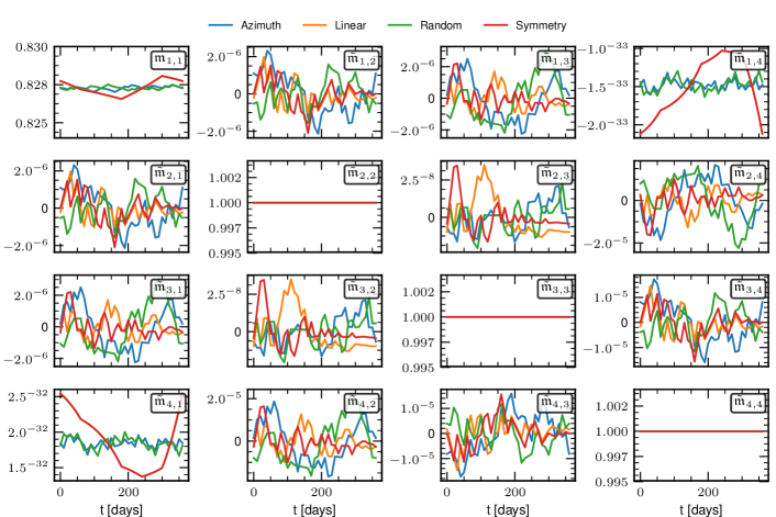
Figure 7: Time dependence of the Mueller matrix characterizing a GTC with conductor oxide for 5000 Å. The time sequence covers a whole primary segment substitution sequence for the four segment substitution sequences (color coded). Note that elements other than $\mathfrak{m}_{1,1}$ represent the reflection corrected value, i.e. $\tilde{\mathfrak{m}}_{i,j}=\mathfrak{m}_{i,j}/\mathfrak{m}_{1,1}$, for each time step.

$$\mathfrak{M}_{\rm E-ELT}^{\rm ideal}=\left(\begin{array}[]{cccc}0.845048&1^{-18}&1^{-19}&1^{-35}\\ 1^{-18}&0.844903&1^{-17}&1^{-18}\\ 1^{-19}&1^{-17}&0.844903&1^{-17}\\ 1^{-33}&1^{-18}&1^{-17}&0.844758\end{array}\right).$$

In both cases, the ideal reflector has no instrumental polarization.

3.3 The effect of oxidation

The next ingredient we factor in is the formation of oxide on the conductor. To do so, we consider a time sequence for the GTC telescope in which we replace a single segment of the primary mirror at a time. By doing so, starting from a completely clean-ideal state, we eventually reach a steady phase in which each individual segment is in a different oxidation stage. We also discuss the different substitution strategies described in Sect. 2.6 , with the aim of emphasizing the importance of this substitution when doing polarimetry in segmented primary mirrors. This is shown in Fig. 7 where this example follows the same inputs as before, i.e. $\sim 10^{7}$ rays at a wavelength of 500 nm. In addition, we change a segment every 10 days so that in 360 days (approximately a year) all the segments have been cleaned once.

In the non-ideal case all the cross-talk terms except I$\leftrightarrow$V are non-zero. In particular, Q$\leftrightarrow$V and U$\leftrightarrow$V terms reach $10^{-5}$, I$\leftrightarrow$Q and I$\leftrightarrow$U terms are of the order of $10^{-6}$, and Q$\leftrightarrow$U term is of the order of $10^{-8}$. This increase of the relative importance of these terms is caused by the larger axial asymmetry induced by having a primary mirror made of segments with different oxidation levels.

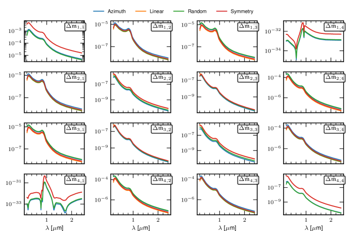
Figure 8: Maximum peak-to-peak variation of the Mueller matrix elements for a complete GTC segment substitution sequence ($\sim$1 year) and its dependence with wavelength. Note that elements other than $\mathfrak{m}_{1,1}$ represent the reflection corrected value, i.e. $\Delta\tilde{\mathfrak{m}}_{i,j}=\Delta\mathfrak{m}_{i,j}/\mathfrak{m}_{1,1}$, for each individual wavelength.

In principle, for typical scientific use cases, one can neglect the Q$\leftrightarrow$U term since this term couples two Stokes parameters that are expected to be already small enough so that the cross level stays well below the noise level. However, I$\leftrightarrow$Q and I$\leftrightarrow$U terms must be taken carefully as linear polarization signals of the order of $10^{-6}$ (and the specific value also depends on wavelength) might be close to the pursued level of the polarimetric sensitivity in the near future for large aperture telescopes. Similarly, strong linearly or circularly polarized sources can introduce significant cross-talk by means of the Q$\leftrightarrow$V and U$\leftrightarrow$V terms. There is no significant improvement on the total amount of cross-talk induced for the different segment substitution sequences considered here. Furthermore, it is not only the largest excursion values that matter but also their variation with time, which can have an important impact on long term studies. In this sense, for all the substitution sequences considered, they give rise to more or less similar cross-talk time variation, i.e. for GTC case there seems to be no preferential way of substituting primary mirror segments.

Concerning the transmittance of the system, we find two different behaviors. The “linear” and “symmetry” segment substitution sequences lead to a pronounced time variation (of the order of $10^{-3}$) with a clear shape. This shape is determined by the distance from the optical axis at which each exchanged segment lies (see Fig. 6 for a reference on the segment behavior as a function of the distance to the optical axis). The first six time steps correspond to the innermost segments, the next six segments are the second closest segments to the optical axis and so on. Due to the larger incidence angle of segments far away from the optical axis, the effect over the transmittance of the system of exchanging an innermost segment is smaller than exchanging an outermost one (see Fig. 6). It is significant that this clear variation on the transmittance of the system has no counterpart on the cross-talk terms. The “azimuth” and “random” substitution methods are characterized by a flatter transmittance behavior all through the time sequence.

As we have previously seen, the polarimetric properties depend upon the wavelength we are considering. In Fig. 8 we explore the effect of the oxidation dependency on wavelength by looking at the maximum peak-to-peak variation of each Mueller matrix element ($\Delta\mathfrak{m}_{i,j}$) on the time sequence needed for a full mirror renovation with wavelength. For all Mueller matrix elements the worst case scenario (the largest peak-to-peak variation) is found for the blue part of the spectrum. It is significant that I$\leftrightarrow$Q and I$\leftrightarrow$U cross-talk terms abruptly improve approximately a $1/3$ fraction at around 0.4 $\mu$m and around an order of magnitude at around 1 $\mu$m. The other relevant cross-talk terms (Q$\leftrightarrow$V, U$\leftrightarrow$V, and Q$\leftrightarrow$U) present a more steady variation with wavelength with an overall improvement when using the largest wavelengths as compared to the blue part of the spectrum.

It is interesting to look to the E-ELT segment substitution sequences as it gives rise to slightly different results, as displayed in Fig. 9. The time sequence is obtained using $\sim 7\times 10^{8}$ rays at 500 nm and changing two segments everyday, so that the primary has been completely renovated in 399 days. First, I$\leftrightarrow$Q and I$\leftrightarrow$U cross-talk terms reach $10^{-6}$, Q$\leftrightarrow$U term reaches $10^{-7}$, while Q$\leftrightarrow$V and U$\leftrightarrow$V can be of the order of $10^{-5}$. The peak amplitude of the Q$\leftrightarrow$U term is an order of magnitude larger than for the GTC case. Second, and in clear contrast to GTC case, different substitution sequences lead to huge differences in the actual value and the time evolution for the various Mueller matrix elements. “Linear” and “symmetry” sequences lead to a smaller peak-to-peak variation of the I$\leftrightarrow$Q, I$\leftrightarrow$U, Q$\leftrightarrow$U, Q$\leftrightarrow$V, and U$\leftrightarrow$V as compared with the “azimuth” and “random” substitution sequences. This means that, in contrast to GTC, for E-ELT it might be interesting to follow specific substitution sequences that minimize the variation with time of the cross-talk terms of the optical system. Finally, diagonal elements do vary very little presenting in the worst case (“linear” and “symmetry”) a 0.1% variation with time.

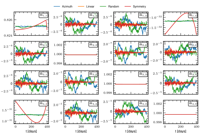
Figure 9: Same as in Fig. 7 for E-ELT.

It is clear that the E-ELT case behaves differently to GTC. The reason is that the number of segments is much larger and so the relative weight of each segment on the overall system is decreased. Consequently, there are more possibilities to develop substitution sequences that minimize the time dependence of the instrumental polarization by increasing the axial symmetry of the system. This is also the reason why the variation with time of the transmittance of E-ELT is much smaller than before, as each segment individually has a smaller effect on the whole system and so the average state of all the segments is more homogeneous than for the GTC. Eventually, there might be some segment substitution sequences for E-ELT that are more suitable when using the telescope for polarimetric studies, specially those that can minimize the I$\leftrightarrow$Q and I$\leftrightarrow$U terms.

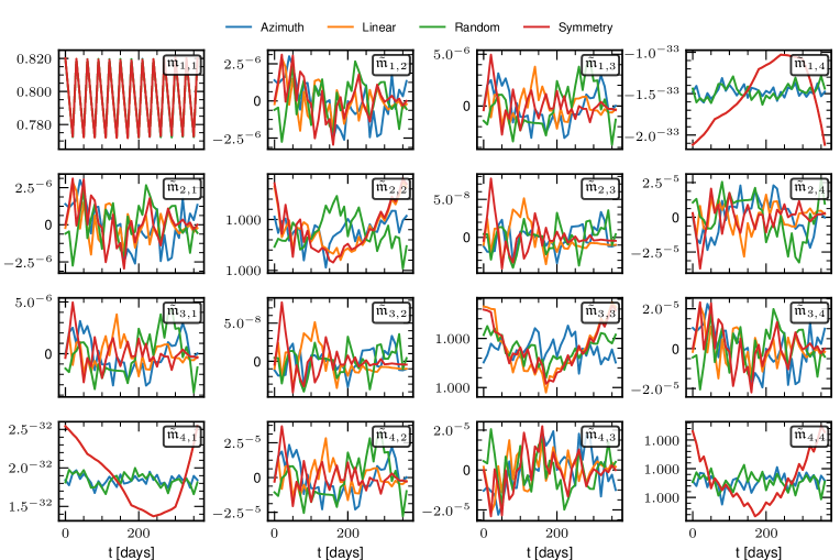
Figure 10: Same as in Fig. 7 including oxidation and dust accumulation over the various segments.

3.4 The effect of dust

This section considers the complete model where we include both oxidation and dust accumulation on the segments of the primary mirror. The model we employ for dust depends only on the rate of dust deposition ($\delta_{0}$) and the efficiency ($\alpha$) and frequency in carbon dioxide snow cleaning. In order to set $\delta_{0}$ and $\alpha$ to realistic values we have used the aging information of GTC segment mirrors as measured by the GTC team (private communication). We set fix $\delta_{0}=3\times 10^{-3}$, $\alpha=90$%, and simulate that a snow cleaning procedure takes place every 30 days. Here, we limit the example to the GTC case because we find no significant effect on the global Mueller matrix when dust is included. Again, we have used 500 nm wavelength and $\sim 10^{7}$ rays and the results are displayed in Fig. 10. The main difference with the case with oxidation only (see Fig. 7) is found in the transmittance of the optical system (see element $\mathfrak{m}_{1,1}$ in Fig. 10), whose shape is dominated by the attenuation as dust is accumulated (the probability of a ray hitting dust and thus being discarded increases) and a sudden improvement of the whole system takes place as a the mirror is cleaned (i.e. it mainly affects to the whole system at once). Actually, cross-talk terms (I$\leftrightarrow$Q, I$\leftrightarrow$U, Q$\leftrightarrow$U, Q$\leftrightarrow$V, and U$\leftrightarrow$V) show no significant variation (neither in values nor in shape) as compared with the case in absence of dust (Fig. 7). The reason for this behavior is that the dust model has a significant degree of axial symmetry. Even though dust has a relative large effect on each segment (as it is clear from the saw-shape transmittance profiles), its effect is quite homogeneous in azimuth and so it has very limited effect on the cross-talk terms. It is to be noticed that this result might be very model dependent. The dust model here employed is quite simple as compared to the dust distribution one might encounter in reality. For instance, one might expect (as it is actually observed at GTC) that the inner mirrors get more dust than the outer ones. It is so because gravity helps maintaining the external mirrors cleaner than the internal ones. Also, the presence of wind micro-currents leads to some axial symmetry loss in the accumulation of dust. Nevertheless, since the latter is a minor effect, one expects a significantly symmetric dust deposition over the primary mirror and in that case, according to the results here found, one would not expect a dramatic change in the cross-talk terms behavior.

4 Conclusion

In summary we have presented a numerical code that estimates the induced instrumental polarization of an optical system. It is done by means of ray tracing and using the Fresnel coefficients and the Stokes formalism. Our focus is to quantify the effect that the axial symmetry breaking around the optical axis has on the polarimetric behavior of the optical system with a segmented primary mirror and an ideal secondary mirror. The usage of segmented primary mirrors allows the sequential replacement of segments whose main effect over the polarimetric behavior of the optical system is an important decrease of the axial symmetry. Here, we have considered the appearance of oxide over the mirror conductor as well as the accumulation of dust. We have found that the different time evolution of these two aging sources (mostly oxidation) leads to the appearance of cross-talk terms that can reach the order of magnitude of the expected polarization signals ($10^{-5}$). The fact that dust has little impact on the polarimetric behavior of the system can be a consequence of the simple model we have used in this work. A detailed-accurate model of dust is extremely difficult to achieve and it is out of the scope for the present work, but even in its current model we think the results are significant for two main reasons: 1- even simple, the model for dust here considered can produce differential polarimetric behavior among the various segments. 2- Employing more complex dust models will not change the symmetry of the problem and thus the overall impact on the polarimetric behavior of the system will be largely reduced . The induced instrumental polarization is wavelength dependent and it is more relevant in the blue part of the spectrum than in the red, where their effect is largely minimized (this effect depends on the refraction index of the conductor being used). An important result is that one can potentially find substitution sequences in telescopes with primary mirrors with a sufficiently small segment-to-mirror area fraction (in this case E-ELT) that clearly reduce the induced polarization terms. We leave the study of these substitution sequences for a future work.

Funding This work has received funding from the European Research Council (ERC) under the European Union’s Horizon 2020 research and innovation programme (SUNMAG, grant agreement 759548), the State Research Agency (AEI) of the Spanish Ministry of Science, Innovation and Universities (MCIU) and the European Regional Development Fund (FEDER) (PGC2018-097611-A-I00 and PGC2018-102108-B-I00).

Acknowledgments We express our appreciation to Antonio Luis Cabrera Lavers and Manuela Abril Abril for their assistance with GTC procedures and measurements. This research has made use of NASA’s Astrophysics Data System Bibliographic Services. We acknowledge the community effort devoted to the development of the following open-source packages that were used in this work: numpy (numpy.org) [18], matplotlib (matplotlib.org)[19], and scipy (scipy.org)[20].

Disclosures The authors declare no conflicts of interest.

Data availability The data that support the findings of this study are available from the corresponding author upon reasonable request.

sample

References

- [1] R. Gilmozzi and J. Spyromilio, “The European Extremely Large Telescope (E-ELT),” \JournalTitleThe Messenger 127, 11 (2007).
- [2] G. H. Sanders, “The Thirty Meter Telescope (TMT): An International Observatory,” \JournalTitleJournal of Astrophysics and Astronomy 34, 81–86 (2013).
- [3] A. S. Brun and M. K. Browning, “Magnetism, dynamo action and the solar-stellar connection,” \JournalTitleLiving Reviews in Solar Physics 14, 4 (2017).
- [4] M. J. Martínez González, A. Asensio Ramos, R. Manso Sainz, R. L. M. Corradi, and F. Leone, “Constraining the shaping mechanism of the Red Rectangle through the spectro-polarimetry of its central star,” \JournalTitleA&A 574, A16 (2015).
- [5] O. Kochukhov, Doppler and Zeeman Doppler Imaging of Stars (2016), vol. 914, p. 177.
- [6] M. I. Carnerero, C. M. Raiteri, M. Villata, J. A. Acosta-Pulido, V. M. Larionov, P. S. Smith, F. D’Ammando, I. Agudo, M. J. Arévalo, R. Bachev, J. Barnes, S. Boeva, V. Bozhilov, D. Carosati, C. Casadio, W. P. Chen, G. Damljanovic, E. Eswaraiah, E. Forné, G. Gantchev, J. L. Gómez, P. A. González-Morales, A. B. Griñón-Marín, T. S. Grishina, M. Holden, S. Ibryamov, M. D. Joner, B. Jordan, S. G. Jorstad, M. Joshi, E. N. Kopatskaya, E. Koptelova, O. M. Kurtanidze, S. O. Kurtanidze, E. G. Larionova, L. V. Larionova, G. Latev, C. Lázaro, R. Ligustri, H. C. Lin, A. P. Marscher, C. Martínez-Lombilla, B. McBreen, B. Mihov, S. N. Molina, J. W. Moody, D. A. Morozova, M. G. Nikolashvili, K. Nilsson, E. Ovcharov, C. Pace, N. Panwar, A. Pastor Yabar, R. L. Pearson, F. Pinna, C. Protasio, N. Rizzi, F. J. Redondo-Lorenzo, G. Rodríguez-Coira, J. A. Ros, A. C. Sadun, S. S. Savchenko, E. Semkov, L. Slavcheva-Mihova, N. Smith, A. Strigachev, Y. V. Troitskaya, I. S. Troitsky, A. A. Vasilyev, and O. Vince, “Dissecting the long-term emission behaviour of the BL Lac object Mrk 421,” \JournalTitleMNRAS 472, 3789–3804 (2017).
- [7] S. V. Berdyugina, A. V. Berdyugin, D. M. Fluri, and V. Piirola, “First Detection of Polarized Scattered Light from an Exoplanetary Atmosphere,” \JournalTitleApJ 673, L83 (2008).
- [8] N. Y. Kiang, S. Domagal-Goldman, M. N. Parenteau, D. C. Catling, Y. Fujii, V. S. Meadows, E. W. Schwieterman, and S. I. Walker, “Exoplanet Biosignatures: At the Dawn of a New Era of Planetary Observations,” \JournalTitleAstrobiology 18, 619–629 (2018).
- [9] C. Capitani, E. Landi Degl’Innocenti, F. Cavallini, G. Ceppatelli, M. Landi Degl’Innocenti, M. Landolfi, and A. Righini, “Polarization properties of a ‘Zeiss-type’ coelostat: The case of the solar tower in Arcetri,” \JournalTitleSol. Phys. 120, 173–191 (1989).
- [10] M. Collados, F. Bettonvil, L. Cavaller, I. Ermolli, B. Gelly, C. Grivel-Gelly, A. Pérez, H. Socas-Navarro, D. Soltau, and R. Volkmer, “European Solar Telescope: project status,” in Ground-based and Airborne Telescopes III, vol. 7733 of Proc. SPIE (2010), p. 77330H.
- [11] C. M. Telesco, D. Ciardi, J. French, C. Ftaclas, K. T. Hanna, D. B. Hon, J. H. Hough, J. Julian, R. Julian, M. Kidger, C. C. Packham, R. K. Pina, F. Varosi, and R. G. Sellar, “CanariCam: a multimode mid-infrared camera for the Gran Telescopio CANARIAS,” in Instrument Design and Performance for Optical/Infrared Ground-based Telescopes, vol. 4841 of Society of Photo-Optical Instrumentation Engineers (SPIE) Conference Series M. Iye and A. F. M. Moorwood, eds. (2003), pp. 913–922.
- [12] S. S. Eikenberry, S. N. Raines, R. D. Stelter, A. Garner, Y. Dallilar, K. Ackley, J. G. Bennett, C. H. Murphey, P. Miller, D. Tooke, L. Williams, B. Chinn, S. A. Mullin, S. L. Schofield, C. D. Warner, F. Varosi, B. Zhao, S. A. Eikenberry, C. Vega, H. V. Donoso, J. Sabater, J. M. Gómez, J. Torra, J. Rosich Minguell, F. Garzón López, N. Cardiel, J. Gallego Maestro, A. Marín-Franch, J. Galipienzo, M. Á. Carrera Astigarraga, G. J. Fitzgerald, I. Prees, T. M. Stolberg, P. A. Kornik, A. N. Ramaprakash, M. P. Burse, S. P. Punnadi, and P. Hammersley, “MIRADAS for the Gran Telescopio Canarias,” in Ground-based and Airborne Instrumentation for Astronomy VI, vol. 9908 of Society of Photo-Optical Instrumentation Engineers (SPIE) Conference Series C. J. Evans, L. Simard, and H. Takami, eds. (2016), p. 99081L.
- [13] J. K. Jennings and B. T. Landesman, Polarization effects from large non-optically flat segmented mirrors (2002), vol. 4489 of Society of Photo-Optical Instrumentation Engineers (SPIE) Conference Series, pp. 89–99.
- [14] R. M. Anche, A. K. Sen, G. C. Anupama, K. Sankarasubramanian, and W. Skidmore, “Analysis of polarization introduced due to the telescope optics of the Thirty Meter Telescope,” \JournalTitleJournal of Astronomical Telescopes, Instruments, and Systems 4, 018003 (2018).
- [15] R. M. Anche, G. C. Anupama, S. Sriram, and K. Sankarasubramanian, “Polarization effects due to the segmented primary mirror of the Thirty Meter Telescope,” in American Astronomical Society Meeting Abstracts #233, vol. 233 of American Astronomical Society Meeting Abstracts (2019), p. 437.01.
- [16] G. Yun, K. Crabtree, and R. A. Chipman, “Three-dimensional polarization ray-tracing calculus I: definition and diattenuation,” \JournalTitleAppl. Opt. 50, 2855 (2011).
- [17] M. Born and E. Wolf, Principles of Optics (1999).
- [18] C. R. Harris, K. J. Millman, S. J. van der Walt, R. Gommers, P. Virtanen, D. Cournapeau, E. Wieser, J. Taylor, S. Berg, N. J. Smith, R. Kern, M. Picus, S. Hoyer, M. H. van Kerkwijk, M. Brett, A. Haldane, J. Fernández del Río, M. Wiebe, P. Peterson, P. Gérard-Marchant, K. Sheppard, T. Reddy, W. Weckesser, H. Abbasi, C. Gohlke, and T. E. Oliphant, “Array programming with NumPy,” \JournalTitleNature 585, 357–362 (2020).
- [19] J. D. Hunter, “Matplotlib: A 2d graphics environment,” \JournalTitleComputing in Science & Engineering 9, 90–95 (2007).
- [20] P. Virtanen, R. Gommers, T. E. Oliphant, M. Haberland, T. Reddy, D. Cournapeau, E. Burovski, P. Peterson, W. Weckesser, J. Bright, S. J. van der Walt, M. Brett, J. Wilson, K. J. Millman, N. Mayorov, A. R. J. Nelson, E. Jones, R. Kern, E. Larson, C. J. Carey, İ. Polat, Y. Feng, E. W. Moore, J. VanderPlas, D. Laxalde, J. Perktold, R. Cimrman, I. Henriksen, E. A. Quintero, C. R. Harris, A. M. Archibald, A. H. Ribeiro, F. Pedregosa, P. van Mulbregt, and SciPy 1.0 Contributors, “SciPy 1.0: Fundamental Algorithms for Scientific Computing in Python,” \JournalTitleNature Methods 17, 261–272 (2020).