Two-body Baryonic $B_{u,d,s}$ and $B_{c}$ to Charmless Final State Decays

Abstract

We study the rates and direct CP violations of two-body baryonic $\bar{B}_{u,d,s}\to{{\rm\bf B}\overline{\rm\bf B}}^{\prime}$ and $B^{-}_{c}\to{{\rm\bf B}\overline{\rm\bf B}}^{\prime}$ decays, where the final state baryons include low-lying octet and decuplet baryons. We incorporate topological amplitude formalism and the factorization approach. Asymptotic relations at large $m_{b}$ are used to simplify decay amplitudes. Using the most up-to-date data on $\bar{B}^{0}\to p\bar{p}$ and $B^{-}\to\Lambda\bar{p}$ decay rates as inputs, rates and direct CP violations of $\bar{B}_{u,d,s}\to{{\rm\bf B}\overline{\rm\bf B}}^{\prime}$ decays are revised and predicted. It is interesting that the results on rates satisfy all existing experimental bounds and some are close to the bounds. Factorization diagrams contribute to penguin-exchange, exchange, annihilation and penguin-annihilation amplitudes. Although the resulting penguin-exchange factorization amplitudes are sizable, the rest suffer from severe chiral suppression and are sensitive to non-factorizable contributions. As the $\bar{B}_{s}\to p\bar{p}$ decay is governed by exchange and penguin annihilation amplitudes, the rate predicted in factorization calculation is very rare, but it can be enhanced by including non-factorizable contributions. The case where the rate is enhanced to saturate the present experimental bound through the enhancement on exchange or penguin-annihilation amplitudes is discussed. As annihilation modes $B^{-}_{c}\to{{\rm\bf B}\overline{\rm\bf B}}^{\prime}$ decays from factorization calculation are found to be very rare, but they can be enhanced by including non-factorizable contributions as well. Small direct CP violations of pure penguin modes in $\Delta S=-1$ $\bar{B}_{u,d,s}\to{{\rm\bf B}\overline{\rm\bf B}}^{\prime}$ decays are robust predictions of the SM, while vanishing direct CP violations of exchange modes in $\bar{B}_{u,d,s}\to{{\rm\bf B}\overline{\rm\bf B}}^{\prime}$ decays and in all $B^{-}_{c}\to{{\rm\bf B}\overline{\rm\bf B}}^{\prime}$ decay modes are null tests of the SM.

I Introduction

Two body baryonic $B$ decays with octet and decuplet baryons have been searched experimentally for some time. The present situation is summarized in Table 1 LHCb:2016nbc ; Belle:2007gob ; Belle:2007lbz ; Belle:2007oni ; LHCb:2017swz ; LHCb:2022lff ; Belle:2019abe ; CLEO:1989xsn ; PDG . So far only the $\bar{B}^{0}\to p\bar{p}$ and $B^{-}\to\Lambda\bar{p}$ modes have been observed LHCb:2016nbc ; LHCb:2017swz . As most of the bounds have not been updated over a decade, experimental progress in this sector from LHCb and Belle II in near future is anticipated.

Theoretically two body baryonic $B$ decays have beed studied in various approaches, including pole model Deshpande:1987nc ; Jarfi:1990ej ; Cheng:2001tr ; Cheng:2001ub , sum rule Chernyak:ag , diquark model Ball:1990fw ; Chang:2001jt , flavor symmetry  Gronau:1987xq ; He:re ; Sheikholeslami:fa ; Luo:2003pv ; Chua:2003it ; Chua:2013zga ; Chua:2016aqy , factorization  He:2006vz ; Hsiao:2014zza ; Hsiao:2019wyd ; Jin:2021onb and some other calculations Cheng:2014qxa . For some recent reviews, see review ; Huang:2021qld .

In this work we will employ the approach of refs. Chua:2003it ; Chua:2013zga ; Chua:2016aqy , which made use of the well established topological amplitude formalism Zeppenfeld:1980ex ; Chau:tk ; Chau:1990ay ; Gronau:1994rj ; Gronau:1995hn ; Chiang:2004nm ; Cheng:2014rfa ; Savage:ub and asymptotic relations Brodsky:1980sx in the large $m_{b}$ limit. Note that the approach successfully predicted the $B^{-}\to\Lambda\bar{p}$ rate Chua:2013zga using the data of $\bar{B}^{0}\to p\bar{p}$ decay Aaij:2013fta .

We shall extend the previous study in several aspects. First, additional topological amplitudes will be introduced in $\bar{B}_{q=u,d,s}\to{\rm\bf B}\overline{\rm\bf B}^{\prime}$ decays with ${\rm\bf B}$ denoting low lying octet and decuplet baryons. Second, some of the topological amplitudes have factorization contributions, which can be calculated using factorization approach. For some important progress of diagrammatic approach with factorization assisted, one is referred to refs. Li:2012cfa ; Qin:2013tje . Note that $\bar{B}_{u,d,s}$ decaying to low lying octet baryon pairs have been studied in refs. Hsiao:2014zza ; Jin:2021onb using factorization approach, but our formalism is different and, consequently, we will be able to extend the study to include all low lying octet and decuplet baryon pairs. Third, we will study $B^{-}_{c}\to{\rm\bf B}\overline{\rm\bf B}^{\prime}$ decays and will give predictions on rates and direct CP violations.

There are accumulating speculations of new physics effects in rare $B$ decays, see, for example, Altmannshofer:2021qrr ; Cornella:2021sby from some recent discussions. Any test of the Standard Model (SM) should be welcomed. In this work we try to identify some robust predictions from SM and null tests of the SM in rare $B$ decays in the baryonic sector.

The layout of this paper is as following. We give the formalism in Sec. II, which is followed by numerical results on rates and direct CP violations of $\bar{B}_{u,d,s}\to{\rm\bf B}\overline{\rm\bf B}^{\prime}$ and $B^{-}_{c}\to{\rm\bf B}\overline{\rm\bf B}^{\prime}$ decays in Sec III. Sec. IV is devoted to discussions and conclusions. We end this paper by two appendices.

Table 1: Experimental results of $\bar{B}_{u,d,s}\to{\rm\bf B}\overline{\rm\bf B}^{\prime}$ branching ratios. The upper limits are at 90% confidence level.

Mode	LHCb	Belle	CLEO	PDG PDG
$B^{-}\to\Lambda\bar{p}$	$(2.4^{+1.0}_{-0.8}\pm 0.3)\times 10^{-7}$ LHCb:2016nbc	$<3.2\times 10^{-7}$ Belle:2007gob		$(2.4^{+1.0}_{-0.9})\times 10^{-7}$
$B^{-}\to\Sigma^{*0}\bar{p}$		$<4.7\times 10^{-7}$ Belle:2007lbz		$<4.7\times 10^{-7}$
$B^{-}\to\Lambda\overline{\Delta^{+}}$		$<8.2\times 10^{-7}$ Belle:2007lbz		$<8.2\times 10^{-7}$
$B^{-}\to\Delta^{0}\bar{p}$		$<1.38\times 10^{-6}$ Belle:2007oni		$<1.38\times 10^{-6}$
$B^{-}\to p\overline{\Delta^{++}}$		$<1.4\times 10^{-7}$ Belle:2007oni		$<1.4\times 10^{-7}$
$\bar{B}^{0}\to p\bar{p}$	$(1.27\pm 0.13\pm 0.05\times 0.03)\times 10^{-8}$ LHCb:2022lff	$<1.1\times 10^{-7}$ Belle:2007gob		$(1.25\pm 0.32)\times 10^{-8}$
$\bar{B}^{0}\to\Sigma^{*+}\bar{p}$		$<2.6\times 10^{-7}$ Belle:2007lbz		$<2.6\times 10^{-7}$
$\bar{B}^{0}\to p\overline{\Delta^{+}},\Delta^{-}\bar{p}$		$<1.6\times 10^{-6}$ Belle:2019abe		$<1.6\times 10^{-6}$
$\bar{B}^{0}\to\Lambda\overline{\Delta^{0}}$		$<9.3\times 10^{-7}$ Belle:2007lbz		$<9.3\times 10^{-7}$
$\bar{B}^{0}\to\Lambda\overline{\Lambda}$		$<3.2\times 10^{-7}$ Belle:2007gob		$<3.2\times 10^{-7}$
$\bar{B}^{0}\to\Delta^{0}\overline{\Delta^{0}}$			$<1.5\times 10^{-3}$ CLEO:1989xsn	$<1.5\times 10^{-3}$
$\bar{B}^{0}\to\Delta^{++}\overline{\Delta^{++}}$			$<1.1\times 10^{-4}$ CLEO:1989xsn	$<1.1\times 10^{-4}$
$\bar{B}^{0}_{s}\to p\bar{p}$	$<4.4\times 10^{-9}$ LHCb:2022lff			$<1.5\times 10^{-8}$

II Formalism

II.1 Topological amplitudes

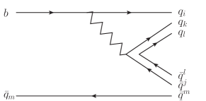
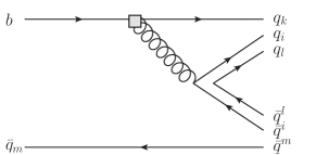
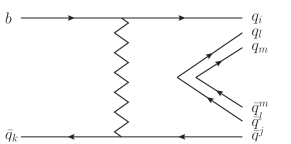
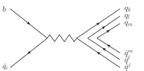
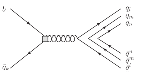
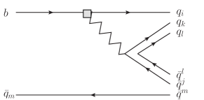
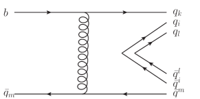
Figure 1: Topological diagrams of (a) $T$ (tree), (b) $P$ (penguin), (c) $E$ ($W$-exchange), (d) $A$ (annihilation), (e) $PA$ (penguin annihilation), (f) $P_{EW}$ (electroweak penguin) and (g) $PE$ (penguin-exchange) amplitudes in $\overline{B}$ to baryon pair decays. These are flavor flow diagrams.

The effective weak Hamiltonian for charmless $\bar{B}_{u,d,s}$ decays is given by Buras

$$H_{\rm eff}=\frac{G_{f}}{\sqrt{2}}\Big{\{}\sum_{r=u,c}V_{qb}V^{*}_{uq}[c_{1}O^{r}_{1}+c_{2}O^{r}_{2}]-V_{tb}V^{*}_{tq}\sum_{i=3}^{10}c_{i}O_{i}\Big{\}}+{\rm H.c.},$$ (1)

where we have $q=d,s$, and

$$O^{r}_{1}=(\bar{r}b)_{V-A}(\bar{q}r)_{V-A},\quad O^{r}_{2}=(\bar{r}_{\alpha}b_{\beta})_{V-A}(\bar{q}_{\beta}r_{\alpha})_{V-A},$$

$$O_{3(5)}=(\bar{q}b)_{V-A}\sum_{q^{\prime}}(\bar{q}^{\prime}q^{\prime})_{V\mp A},\quad O_{4(6)}=(\bar{q}_{\alpha}b_{\beta})_{V-A}\sum_{q^{\prime}}(\bar{q}_{\beta}^{\prime}q_{\alpha}^{\prime})_{V\mp A},$$

$$O_{7(9)}=\frac{3}{2}(\bar{q}b)_{V-A}\sum_{q^{\prime}}e_{q^{\prime}}(\bar{q}^{\prime}q^{\prime})_{V\pm A},\quad O_{8(10)}=\frac{3}{2}(\bar{q}_{\alpha}b_{\beta})_{V-A}\sum_{q^{\prime}}e_{q^{\prime}}(\bar{q}_{\beta}^{\prime}q_{\alpha}^{\prime})_{V\pm A},$$ (2)

with $O_{3-6}$ the QCD penguin operators, $O_{7-10}$ the electroweak penguin operators, and $(\bar{q}^{\prime}q)_{V\pm A}\equiv\bar{q}^{\prime}\gamma_{\mu}(1+\pm\gamma_{5})q$. The next-to-leading order Wilson coefficients,

$$c_{1}=1.081,\,c_{2}=-0.190,\,c_{3}=0.014,\,c_{4}=-0.036,\,c_{5}=0.009,\,c_{6}=-0.042,$$

$$c_{7}=-0.011\alpha_{EM},\,c_{8}=0.060\alpha_{EM},\,c_{9}=-1.254\alpha_{EM},\,c_{10}=0.223\alpha_{EM},$$ (3)

are evaluated in the naive dimensional regularization scheme at scale $\mu=4.2$GeV Beneke:2001ev .

We follow the approach of Chua:2003it ; Chua:2013zga ; Chua:2016aqy to decompose $\bar{B}_{q}\to{{\cal B}\overline{\cal B}}$, ${{\cal B}\overline{\cal D}}$, ${{\cal D}\overline{\cal B}}$ and ${{\cal D}\overline{\cal D}}$ decay amplitudes, with $q=u,d,s$, ${\cal B}$ and ${\cal D}$ denoting low-lying octet and decuplet baryons, into topological amplitudes. We have tree ($T$), penguin ($P$), electroweak penguin($P_{EW}$), $W$-exchange ($E$) annihilation, penguin-annihilation ($PA$) and penguin-exchange ($PE$) amplitudes, see Fig. 1 for the corresponding diagrams. For $\Delta S=0$ transition, the tree (${\cal O}_{T}=O_{1,2}$), penguin (${\cal O}_{P}=O_{3-6}$) and electroweak penguin (${\cal O}_{EWP}=O_{7-10}$) operators in Hamiltonian has the following flavor structure,

$${\cal O}_{T}\sim(\bar{u}b)(\bar{d}u)=H^{ik}_{j}(\bar{q}_{i}b)(\bar{q}_{k}q^{j}),\quad{\cal O}_{P}\sim(\bar{d}b)(\bar{q}_{i}q^{i})=H^{k}(\bar{q}_{k}b)(\bar{q}_{i}q^{i}),$$

$${\cal O}_{EWP}\sim Q_{j}(\bar{d}b)(\bar{q}_{j}q^{j})=H_{EW}{}^{ik}_{j}(\bar{q}_{i}b)(\bar{q}_{k}q^{j}),$$ (4)

with

$$H^{12}_{1}=1=H^{2},H_{EW}{}^{2k}_{j}=Q_{j}\delta^{k}_{j}\,\,\,{\rm otherwise}\,\,\,H^{ik}_{j}=H_{EW}{}^{ik}_{j}=H^{k}=0.$$ (5)

Following ref. Chua:2003it by suitably matching the $q_{k}q_{i}q_{l}$ flavor to decuplet and octet baryon fields, we obtain the following effective Hamiltonian for $\bar{B}_{q}\to{{\cal D}\overline{\cal D}},{{\cal B}\overline{\cal D}},{{\cal D}\overline{\cal B}}$ and ${{\cal B}\overline{\cal B}}$ decays,

$$H^{{\cal D}\overline{\cal D}}_{\rm eff} = 6\,T_{{\cal D}\overline{\cal D}}\,\overline{B}_{m}H^{ik}_{j}\overline{\cal D}_{ikl}{\cal D}^{ljm}+6P_{{\cal D}\overline{\cal D}}\,\overline{B}_{m}H^{k}\overline{\cal D}_{kil}{\cal D}^{lim}+6E_{{\cal D}\overline{\cal D}}\,\overline{B}_{k}H^{ik}_{j}\overline{\cal D}_{ilm}{\cal D}^{mlj}$$ (6)

$$+6A_{{\cal D}\overline{\cal D}}\,\overline{B}_{i}H^{ik}_{j}\overline{\cal D}_{klm}{\cal D}^{mlj}+2PA_{{\cal D}\overline{\cal D}}\,\overline{B}_{k}H^{k}\overline{\cal D}_{lmn}{\cal D}^{nml}+6\,P_{EW{\cal D}\overline{\cal D}}\,\overline{B}_{m}H^{ik}_{EW\,j}\overline{\cal D}_{ikl}{\cal D}^{ljm}$$

$$+6PE_{{\cal D}\overline{\cal D}}\,\overline{B}_{m}H^{k}\overline{\cal D}_{kil}{\cal D}^{lim},$$

$$H^{{\cal B}\overline{\cal D}}_{\rm eff} = -\sqrt{6}\,T_{1{{\cal B}\overline{\cal D}}}\,\overline{B}_{m}H^{ik}_{j}\epsilon_{ika}\overline{\cal B}^{a}_{l}{\cal D}^{ljm}-2\sqrt{6}\,T_{2{{\cal B}\overline{\cal D}}}\,\overline{B}_{m}H^{ik}_{j}\epsilon_{akl}\overline{\cal B}^{a}_{i}{\cal D}^{ljm}$$ (7)

$$-\sqrt{6}P_{{\cal B}\overline{\cal D}}\,\overline{B}_{m}H^{k}\epsilon_{kia}\overline{\cal B}^{a}_{l}{\cal D}^{lim}-\sqrt{6}E_{{\cal B}\overline{\cal D}}\,\overline{B}_{k}H^{ik}_{j}\epsilon_{ila}\overline{\cal B}^{a}_{m}{\cal D}^{mlj}-\sqrt{6}A_{{\cal B}\overline{\cal D}}\,\overline{B}_{i}H^{ik}_{j}\epsilon_{kla}\overline{\cal B}^{a}_{m}{\cal D}^{mlj}$$

$$-\sqrt{6}\,P_{1EW{{\cal B}\overline{\cal D}}}\,\overline{B}_{m}H_{EW}{}^{ik}_{j}\epsilon_{ika}\overline{\cal B}^{a}_{l}{\cal D}^{ljm}-2\sqrt{6}\,P_{2EW{{\cal B}\overline{\cal D}}}\,\overline{B}_{m}H_{EW}{}^{ik}_{j}\epsilon_{akl}\overline{\cal B}^{a}_{i}{\cal D}^{ljm}$$

$$-\sqrt{6}PE_{{\cal B}\overline{\cal D}}\,\overline{B}_{m}H^{k}\epsilon_{kia}\overline{\cal B}^{a}_{l}{\cal D}^{lim},$$

$$H^{{\cal D}\overline{\cal B}}_{\rm eff} = -\sqrt{6}\,T_{1{{\cal D}\overline{\cal B}}}\,\overline{B}_{m}H^{ik}_{j}\overline{\cal D}_{ikl}\epsilon^{ljb}{\cal B}^{m}_{b}+\sqrt{6}\,T_{2{{\cal D}\overline{\cal B}}}\,\overline{B}_{m}H^{ik}_{j}\overline{\cal D}_{ikl}\epsilon^{bjm}{\cal B}^{l}_{b}$$ (8)

$$+\sqrt{6}P_{{\cal D}\overline{\cal B}}\,\overline{B}_{m}H^{k}\overline{\cal D}_{kil}\epsilon^{bim}{\cal B}^{l}_{b}+\sqrt{6}E_{{\cal D}\overline{\cal B}}\,\overline{B}_{k}H^{ik}_{j}\overline{\cal D}_{ilm}\epsilon^{bli}{\cal B}^{m}_{b}+\sqrt{6}A_{{\cal D}\overline{\cal B}}\,\overline{B}_{i}H^{ik}_{j}\overline{\cal D}_{klm}\epsilon^{bli}{\cal B}^{m}_{b}$$

$$-\sqrt{6}\,P_{1EW{{\cal D}\overline{\cal B}}}\,\overline{B}_{m}H_{EW}{}^{ik}_{j}\overline{\cal D}_{ikl}\epsilon^{ljb}{\cal B}^{m}_{b}+\sqrt{6}\,P_{2EW{{\cal D}\overline{\cal B}}}\,\overline{B}_{m}H_{EW}{}^{ik}_{j}\overline{\cal D}_{ikl}\epsilon^{bjm}{\cal B}^{l}_{b}$$

$$+\sqrt{6}PE_{{\cal D}\overline{\cal B}}\,\overline{B}_{m}H^{k}\overline{\cal D}_{kil}\epsilon^{bim}{\cal B}^{l}_{b},$$

and

$$H^{{\cal B}\overline{\cal B}}_{\rm eff} = T_{1{{\cal B}\overline{\cal B}}}\,\overline{B}_{m}H^{ik}_{j}\epsilon_{ika}\overline{\cal B}^{a}_{l}\epsilon^{ljb}{\cal B}^{m}_{b}-T_{2{{\cal B}\overline{\cal B}}}\,\overline{B}_{m}H^{ik}_{j}\epsilon_{ika}\overline{\cal B}^{a}_{l}\epsilon^{bjm}{\cal B}^{l}_{b}$$ (9)

$$+2T_{3{{\cal B}\overline{\cal B}}}\,\overline{B}_{m}H^{ik}_{j}\epsilon_{akl}\overline{\cal B}^{a}_{i}\epsilon^{ljb}{\cal B}^{m}_{b}-2T_{4{{\cal B}\overline{\cal B}}}\,\overline{B}_{m}H^{ik}_{j}\epsilon_{akl}\overline{\cal B}^{a}_{i}\epsilon^{bjm}{\cal B}^{l}_{b}$$

$$-5P_{1{{\cal B}\overline{\cal B}}}\,\overline{B}_{m}H^{k}\epsilon_{kia}\overline{\cal B}^{a}_{l}\epsilon^{lib}{\cal B}^{m}_{b}-P_{2{{\cal B}\overline{\cal B}}}\,\overline{B}_{m}H^{k}\epsilon_{kia}\overline{\cal B}^{a}_{l}\epsilon^{bim}{\cal B}^{l}_{b}$$

$$-5E_{1{{\cal B}\overline{\cal B}}}\,\overline{B}_{k}H^{ik}_{j}\epsilon_{ila}\overline{\cal B}^{a}_{m}\epsilon^{mlb}{\cal B}^{j}_{b}-E_{2{{\cal B}\overline{\cal B}}}\,\overline{B}_{k}H^{ik}_{j}\epsilon_{ila}\overline{\cal B}^{a}_{m}\epsilon^{blj}{\cal B}^{l}_{m}$$

$$-5A_{1{{\cal B}\overline{\cal B}}}\,\overline{B}_{i}H^{ik}_{j}\epsilon_{kla}\overline{\cal B}^{a}_{m}\epsilon^{mlb}{\cal B}^{j}_{b}-A_{2{{\cal B}\overline{\cal B}}}\,\overline{B}_{i}H^{ik}_{j}\epsilon_{kla}\overline{\cal B}^{a}_{m}\epsilon^{blj}{\cal B}^{l}_{m}$$

$$+P_{1EW{{\cal B}\overline{\cal B}}}\,\overline{B}_{m}H_{EW}{}^{ik}_{j}\epsilon_{ika}\overline{\cal B}^{a}_{l}\epsilon^{ljb}{\cal B}^{m}_{b}-P_{2EW{{\cal B}\overline{\cal B}}}\,\overline{B}_{m}H_{EW}{}^{ik}_{j}\epsilon_{ika}\overline{\cal B}^{a}_{l}\epsilon^{bjm}{\cal B}^{l}_{b}$$

$$+2P_{3EW{{\cal B}\overline{\cal B}}}\,\overline{B}_{m}H_{EW}{}^{ik}_{j}\epsilon_{akl}\overline{\cal B}^{a}_{i}\epsilon^{ljb}{\cal B}^{m}_{b}-2P_{4EW{{\cal B}\overline{\cal B}}}\,\overline{B}_{m}H_{EW}{}^{ik}_{j}\epsilon_{akl}\overline{\cal B}^{a}_{i}\epsilon^{bjm}{\cal B}^{l}_{b}$$

$$-PA_{{\cal B}\overline{\cal B}}\,\overline{B}_{k}H^{k}\epsilon_{lma}\overline{\cal B}^{a}_{n}\epsilon^{nmb}{\cal B}^{l}_{b}-5PE_{1{{\cal B}\overline{\cal B}}}\,\overline{B}_{m}H^{k}\epsilon_{kia}\overline{\cal B}^{a}_{l}\epsilon^{lib}{\cal B}^{m}_{b}$$

$$-PE_{2{{\cal B}\overline{\cal B}}}\,\overline{B}_{m}H^{k}\epsilon_{kia}\overline{\cal B}^{a}_{l}\epsilon^{bim}{\cal B}^{l}_{b}.$$

with ${\overline{B}}_{m}=\left(B^{-},\overline{B}{}^{0},\overline{B}{}^{0}_{s}\right)$, ${\cal D}^{111}=\Delta^{++}$, ${\cal D}^{112}=\Delta^{+}/\sqrt{3}$, ${\cal D}^{122}=\Delta^{0}/\sqrt{3}$, ${\cal D}^{222}=\Delta^{-}$, ${\cal D}^{113}=\Sigma^{*-}/\sqrt{3}$, ${\cal D}^{123}=\Sigma^{*0}/\sqrt{6}$, ${\cal D}^{223}=\Sigma^{*-}/\sqrt{3}$, ${\cal D}^{133}=\Xi^{*0}/\sqrt{3}$, ${\cal D}^{233}=\Xi^{*-}/\sqrt{3}$ ${\cal D}^{333}=\Omega^{-}$, and

$${\mathcal{B}}=\left(\begin{array}[]{ccc}{{\Sigma^{0}}\over\sqrt{2}}+{{\Lambda}\over\sqrt{6}}&{\Sigma^{+}}&{p}\\ {\Sigma^{-}}&-{{\Sigma^{0}}\over\sqrt{2}}+{{\Lambda}\over\sqrt{6}}&{n}\\ {\Xi^{-}}&{\Xi^{0}}&-\sqrt{2\over 3}{\Lambda}\end{array}\right),$$ (13)

(see, for example text ). Note that the penguin exchange amplitudes, $PE$ are new and the coefficients of $PA$ are adjusted (by a factor of $1/3$) for later purpose.

The above formalism can be extended to study $B^{-}_{c}\to{\rm\bf B}\overline{\rm\bf B}^{\prime}$ decays. The Hamiltonian governing the decays has the following flavor structure,

$${\cal O}_{T}\sim(\bar{c}b)(\bar{d}u)=H^{ck}_{j}(\bar{c}b)(\bar{q}_{k}q^{j}),\quad H^{c2}_{1}=1,\,\,\,{\rm otherwise}\,\,\,H^{ck}_{j}=0.$$ (14)

Hence the effective Hamiltonian for $\bar{B}_{c}\to{{\cal D}\overline{\cal D}},{{\cal B}\overline{\cal D}},{{\cal D}\overline{\cal B}}$ and ${{\cal B}\overline{\cal B}}$ decays can be constructed similarly giving

$$H^{c{{\cal D}\overline{\cal D}}}_{\rm eff} = 6A^{c}_{{\cal D}\overline{\cal D}}\,\overline{B}_{c}H^{ck}_{j}\overline{\cal D}_{klm}{\cal D}^{mlj},$$ (15)

$$H^{c{{\cal D}\overline{\cal B}}}_{\rm eff} = \sqrt{6}A^{c}_{{\cal D}\overline{\cal B}}\,\overline{B}_{c}H^{ck}_{j}\overline{\cal D}_{klm}\epsilon^{bli}{\cal B}^{m}_{b},$$ (16)

$$H^{c{{\cal B}\overline{\cal D}}}_{\rm eff} = -\sqrt{6}A^{c}_{{\cal B}\overline{\cal D}}\,\overline{B}_{c}H^{ck}_{j}\epsilon_{kla}\overline{\cal B}^{a}_{m}{\cal D}^{mlj},$$ (17)

and

$$H^{c{{\cal B}\overline{\cal B}}}_{\rm eff} = -5A^{c}_{1{{\cal B}\overline{\cal B}}}\,\overline{B}_{c}H^{ck}_{j}\epsilon_{kla}\overline{\cal B}^{a}_{m}\epsilon^{mlb}{\cal B}^{j}_{b}-A^{c}_{2{{\cal B}\overline{\cal B}}}\,\overline{B}_{c}H^{ck}_{j}\epsilon_{kla}\overline{\cal B}^{a}_{m}\epsilon^{blj}{\cal B}^{l}_{m}.$$ (18)

The above results for $\bar{B}_{u,d,s}$ and $B^{-}_{c}$ decays are for $\Delta S=0$ transitions. In the case of $\Delta S=-1$ transition, we put a prime in topological amplitudes and use $H^{13}_{1}=1=H^{3}$, $H_{EW}{}^{3k}_{j}=Q_{j}\delta^{k}_{j}$ and $H^{c3}_{1}=1$ for non-vanishing elements, instead.

The $\bar{B}_{q},\bar{B}_{c}\to{{\cal B}\overline{\cal B}}^{\prime},{{\cal B}\overline{\cal D}}^{\prime},{{\cal D}\overline{\cal B}}^{\prime}$ and ${{\cal D}\overline{\cal D}}^{\prime}$ decay amplitudes obtained using these effective Hamiltonian are collected in App. A. Since the flavor flow structures of penguin exchange diagrams and penguin diagrams are identical, see Fig. 1 (b) and (g), these two topological amplitudes always occur in the combination of $P^{(\prime)}_{i}+PE^{(\prime)}_{i}$ in the decay amplitudes. It should be noted that although the above constructions make use of SU(3) symmetry, they are use as tools, as bookkeeping devices, to obtain flavor flow structure of the decay amplitudes. Once the flavor flow structure is obtained, SU(3) breaking effects, through masses, decay constants and so on, in these topological amplitudes can be imposed. Note that annihilation diagrams only exist in $B^{-}$ and $B^{-}_{c}$ decays, while exchange diagrams only exist in $B^{0}_{d}$ and $B^{0}_{s}$ decays and penguin-annihilation diagrams only exist in $\bar{B}^{0}_{d(s)}\to{{\cal B}\overline{\cal B}}$ and ${{\cal D}\overline{\cal D}}$ decays, where the final state anti-baryon is the anti-particle of the associated final state baryon.

II.2 Factorization contributions to $A^{(\prime)}$, $E^{(\prime)}$, $PE^{(\prime)}$ and $PA^{(\prime)}$

A typical factorizable $\bar{B}\to{\rm\bf B}\overline{\rm\bf B}^{\prime}$ decay amplitude has the following expression, which is similar to the mesonic case Beneke:2001ev :

$$A_{\rm fac}\left(\bar{B}\to{\rm\bf B}\overline{\rm\bf B}^{\prime}\right) = \frac{G_{F}}{\sqrt{2}}\bigg{\{}V_{ub}V_{uq}^{*}[a_{1}(\bar{q}u)_{V-A}\otimes(\bar{u}b)_{V-A}+a_{2}(\bar{u}u)_{V-A}\otimes(\bar{q}b)_{V-A}]$$ (19)

$$-V_{tb}V_{tq}^{*}\Big{[}a_{3}\sum_{q^{\prime}}(\bar{q}^{\prime}q^{\prime})_{V-A}\otimes(\bar{q}b)_{V-A}+a_{4}\sum_{q^{\prime}}(\bar{q}q^{\prime})_{V-A}\otimes(\bar{q}^{\prime}b)_{V-A}$$

$$\quad+a_{5}\sum_{q^{\prime}}(\bar{q}^{\prime}q^{\prime})_{V+A}\otimes(\bar{q}b)_{V-A}-2a_{6}\sum_{q^{\prime}}(\bar{q}q^{\prime})_{S+P}\otimes(\bar{q}^{\prime}b)_{S-P}\Big{]}\bigg{\}}\,,$$

where ${\cal O}_{1}\otimes{\cal O}_{2}$ is the shorthand of

$${\cal O}_{1}\otimes{\cal O}_{2}\equiv\langle{\rm\bf B}\overline{\rm\bf B}^{\prime}|{\cal O}_{1}|0\rangle\langle 0|{\cal O}_{2}|\bar{B}\rangle$$ (20)

and we neglect the contributions from electroweak penguin operators in the factorization calculation. Note that in factorization calculation the electroweak penguin operators contribute to electroweak-exchange and electroweak-annihilation diagrams, which are negligible comparing to the topological amplitudes generated from tree and strong penguin operators, and these topological amplitudes are not considered in this work. In the leading order, the coefficients $a_{i}$ are defined in terms of the effective Wilson coefficients $c_{i}$ as

$$a^{\rm LO}_{i={\rm odd}} \equiv c_{i}+c_{i+1}/N_{c},$$

$$a^{\rm LO}_{i={\rm even}} \equiv c_{i}+c_{i-1}/N_{c}.$$ (21)

Contributions beyond the leading order will neglected in this work. It will be useful to express the above factorization amplitudes according to the decaying mesons, giving

$$A_{\rm fac}\left(B^{-}\to{\rm\bf B}\overline{\rm\bf B}^{\prime}\right) = \frac{G_{F}}{\sqrt{2}}\bigg{\{}V_{ub}V_{uq}^{*}a_{1}(\bar{q}u)_{V-A}\otimes(\bar{u}b)_{V-A}-V_{tb}V_{tq}^{*}\Big{[}a_{4}(\bar{q}u)_{V-A}\otimes(\bar{u}b)_{V-A}$$ (22)

$$\quad-2a_{6}(\bar{q}u)_{S+P}\otimes(\bar{u}b)_{S-P}\Big{]}\bigg{\}}\,,$$

$$A_{\rm fac}\left(\bar{B}_{d}\to{\rm\bf B}\overline{\rm\bf B}^{\prime}\right) = \frac{G_{F}}{\sqrt{2}}\bigg{\{}V_{ub}V_{uq}^{*}a_{2}(\bar{u}u)_{V-A}\otimes(\bar{q}b)_{V-A}\delta_{qd}$$ (23)

$$-V_{tb}V_{tq}^{*}\Big{[}a_{3}\sum_{q^{\prime}}(\bar{q}^{\prime}q^{\prime})_{V-A}\otimes(\bar{q}b)_{V-A}\delta_{qd}+a_{4}(\bar{q}d)_{V-A}\otimes(\bar{d}b)_{V-A}$$

$$\quad+a_{5}\sum_{q^{\prime}}(\bar{q}^{\prime}q^{\prime})_{V+A}\otimes(\bar{q}b)_{V-A}\delta_{qd}-2a_{6}(\bar{q}d)_{S+P}\otimes(\bar{d}b)_{S-P}\Big{]}\bigg{\}}\,,$$

$$A_{\rm fac}\left(\bar{B}_{s}\to{\rm\bf B}\overline{\rm\bf B}^{\prime}\right) = \frac{G_{F}}{\sqrt{2}}\bigg{\{}V_{ub}V_{uq}^{*}a_{2}(\bar{u}u)_{V-A}\otimes(\bar{q}b)_{V-A}\delta_{qs}$$ (24)

$$-V_{tb}V_{tq}^{*}\Big{[}a_{3}\sum_{q^{\prime}}(\bar{q}^{\prime}q^{\prime})_{V-A}\otimes(\bar{q}b)_{V-A}\delta_{qs}+a_{4}(\bar{q}s)_{V-A}\otimes(\bar{s}b)_{V-A}$$

$$\quad+a_{5}\sum_{q^{\prime}}(\bar{q}^{\prime}q^{\prime})_{V+A}\otimes(\bar{q}b)_{V-A}\delta_{qs}-2a_{6}(\bar{q}s)_{S+P}\otimes(\bar{s}b)_{S-P}\Big{]}\bigg{\}}\,,$$

and

$$A_{\rm fac}\left(B^{-}_{c}\to{\rm\bf B}\overline{\rm\bf B}^{\prime}\right) = \frac{G_{F}}{\sqrt{2}}V_{cb}V_{uq}^{*}a_{1}(\bar{q}u)_{V-A}\otimes(\bar{c}b)_{V-A}.$$ (25)

By comparing these amplitudes with the topological amplitudes given in App. A, we have the following correspondence between topological amplitudes and the factorization amplitudes:

$$c^{A}_{i,B^{-}_{u}\to{\rm\bf B}\overline{\rm\bf B}^{\prime}}A_{i,B^{-}_{u}\to{\rm\bf B}\overline{\rm\bf B}^{\prime}} = \frac{G_{F}}{\sqrt{2}}V_{ub}V_{ud}^{*}\,a_{1}(\bar{d}u)_{V-A}\otimes(\bar{u}b)_{V-A},$$

$$c^{A^{c}}_{i,B^{-}_{c}\to{\rm\bf B}\overline{\rm\bf B}^{\prime}}A^{c}_{i,B^{-}_{c}\to{\rm\bf B}\overline{\rm\bf B}^{\prime}} = \frac{G_{F}}{\sqrt{2}}V_{cb}V_{ud}^{*}a_{1}(\bar{d}u)_{V-A}\otimes(\bar{c}b)_{V-A},$$

$$c^{E}_{i,\bar{B}_{d}\to{\rm\bf B}\overline{\rm\bf B}^{\prime}}E_{i,\bar{B}_{d}\to{\rm\bf B}\overline{\rm\bf B}^{\prime}} = \frac{G_{F}}{\sqrt{2}}V_{ub}V_{ud}^{*}a_{2}(\bar{u}u)_{V-A}\otimes(\bar{d}b)_{V-A},$$

$$c^{PE}_{i,\bar{B}_{q^{\prime\prime}}\to{\rm\bf B}\overline{\rm\bf B}^{\prime}}PE_{i,\bar{B}_{q^{\prime\prime}}\to{\rm\bf B}\overline{\rm\bf B}^{\prime}} = -\frac{G_{F}}{\sqrt{2}}V_{tb}V_{td}^{*}\,[a_{4}(\bar{d}q^{\prime\prime})_{V-A}\otimes(\bar{q}^{\prime\prime}b)_{V-A}-2a_{6}(\bar{d}q^{\prime\prime})_{S+P}\otimes(\bar{q}^{\prime\prime}b)_{S-P}],$$

$$c^{PA}_{B^{-}_{d}\to{\rm\bf B}\overline{\rm\bf B}^{\prime}}PA_{B^{-}_{d}\to{\rm\bf B}\overline{\rm\bf B}^{\prime}} = -\frac{G_{F}}{\sqrt{2}}V_{tb}V_{td}^{*}\,[a_{3}\sum_{q^{\prime}}(\bar{q}^{\prime}q^{\prime})_{V-A}\otimes(\bar{d}b)_{V-A}$$ (26)

$$\quad+a_{5}\sum_{q^{\prime}}(\bar{q}^{\prime}q^{\prime})_{V+A}\otimes(\bar{d}b)_{V-A}],$$

for $\Delta S=0$ transition, and

$$c^{A^{\prime}}_{i,B^{-}_{u}\to{\rm\bf B}\overline{\rm\bf B}^{\prime}}A^{\prime}_{i,B^{-}_{u}\to{\rm\bf B}\overline{\rm\bf B}^{\prime}} = \frac{G_{F}}{\sqrt{2}}V_{ub}V_{us}^{*}\,a_{1}(\bar{s}u)_{V-A}\otimes(\bar{u}b)_{V-A},$$

$$c^{A^{\prime c}}_{i,B^{-}_{c}\to{\rm\bf B}\overline{\rm\bf B}^{\prime}}A^{\prime c}_{i,B^{-}_{c}\to{\rm\bf B}\overline{\rm\bf B}^{\prime}} = \frac{G_{F}}{\sqrt{2}}V_{cb}V_{us}^{*}a_{1}(\bar{s}u)_{V-A}\otimes(\bar{c}b)_{V-A},$$

$$c^{E^{\prime}}_{i,\bar{B}_{s}\to{\rm\bf B}\overline{\rm\bf B}^{\prime}}E^{\prime}_{i,\bar{B}_{s}\to{\rm\bf B}\overline{\rm\bf B}^{\prime}} = \frac{G_{F}}{\sqrt{2}}V_{ub}V_{us}^{*}a_{2}(\bar{u}u)_{V-A}\otimes(\bar{s}b)_{V-A},$$

$$c^{PE^{\prime}}_{i,\bar{B}_{q^{\prime\prime}}\to{\rm\bf B}\overline{\rm\bf B}^{\prime}}PE^{\prime}_{i,\bar{B}_{q^{\prime\prime}}\to{\rm\bf B}\overline{\rm\bf B}^{\prime}} = -\frac{G_{F}}{\sqrt{2}}V_{tb}V_{ts}^{*}\,[a_{4}(\bar{s}q^{\prime\prime})_{V-A}\otimes(\bar{q}^{\prime\prime}b)_{V-A}-2a_{6}(\bar{s}q^{\prime\prime})_{S+P}\otimes(\bar{q}^{\prime\prime}b)_{S-P}],$$

$$c^{PA^{\prime}}_{B^{-}_{s}\to{\rm\bf B}\overline{\rm\bf B}^{\prime}}PA^{\prime}_{B^{-}_{s}\to{\rm\bf B}\overline{\rm\bf B}^{\prime}} = -\frac{G_{F}}{\sqrt{2}}V_{tb}V_{ts}^{*}\,[a_{3}\sum_{q^{\prime}}(\bar{q}^{\prime}q^{\prime})_{V-A}\otimes(\bar{s}b)_{V-A}$$ (27)

$$\quad+a_{5}\sum_{q^{\prime}}(\bar{q}^{\prime}q^{\prime})_{V+A}\otimes(\bar{s}b)_{V-A}],$$

for $\Delta S=-1$ transition, where the constants $c$ are the Clebsch-Gordan coefficients accompanying with the topological amplitudes in the corresponding $\bar{B}_{q}\to{\rm\bf B}\overline{\rm\bf B}^{\prime}$ decay amplitudes as shown in App. A and summations over $i$, if necessary, are understood.

Table 2: The coefficients $(e_{1},e_{2},e_{3})$ and $r_{{\rm\bf B}\overline{\rm\bf B}}$ for ${{\cal D}\overline{\cal D}}$ and ${{\cal B}\overline{\cal B}}$ final states.

${\rm\bf B}\overline{\rm\bf B}$	$(e_{1},e_{2},e_{3})$	$r_{{\rm\bf B}\overline{\rm\bf B}}$	${\rm\bf B}\overline{\rm\bf B}$	$(e_{1},e_{2},e_{3})$	$r_{{\rm\bf B}\overline{\rm\bf B}}$
$\Delta^{++}\overline{\Delta^{++}}$	$(1,0,0)$	0.022	$\Delta^{+}\overline{\Delta^{+}}$	$\frac{1}{3}(2,1,0)$	0.030
$\Delta^{0}\overline{\Delta^{0}}$	$\frac{1}{3}(1,2,0)$	0.038	$\Delta^{-}\overline{\Delta^{-}}$	$(0,1,0)$	0.047
$\Sigma^{*+}\overline{\Sigma^{*+}}$	$\frac{1}{3}(2,0,1)$	0.325	$\Sigma^{*0}\overline{\Sigma^{*0}}$	$\frac{1}{3}(1,1,1)$	0.333
$\Sigma^{*-}\overline{\Sigma^{*-}}$	$\frac{1}{3}(0,2,1)$	0.342	$\Xi^{*0}\overline{\Xi^{*0}}$	$\frac{1}{3}(1,0,2)$	0.628
$\Xi^{*-}\overline{\Xi^{*-}}$	$\frac{1}{3}(0,1,2)$	0.637	$\Omega^{-}\overline{\Omega^{-}}$	$(0,0,1)$	0.932
$p\,\overline{p}$	$\frac{1}{3}(4,-1,0)$	0.013	$n\,\overline{n}$	$\frac{1}{3}(-1,4,0)$	0.055
$\Sigma^{+}\,\overline{\Sigma^{+}}$	$\frac{1}{3}(4,0,-1)$	$-0.282$	$\Sigma^{0}\,\overline{\Sigma^{0}}$	$\frac{1}{3}(2,2,-1)$	$-0.265$
$\Sigma^{-}\,\overline{\Sigma^{-}}$	$\frac{1}{3}(0,4,-1)$	$-0.248$	$\Lambda\,\overline{\Lambda}$	$(0,0,1)$	$0.932$
$\Xi^{0}\,\overline{\Xi^{0}}$	$\frac{1}{3}(-1,0,4)$	1.235	$\Xi^{-}\,\overline{\Xi^{-}}$	$\frac{1}{3}(0,-1,4)$	1.226

Using

$$\langle 0|(\bar{q}b)_{V-A}|\bar{B}_{q}\rangle=-if_{B_{q}}p_{\mu}$$ (28)

and equations of motions, the matrix elements in the above equations can be evaluated as

$$\langle{\rm\bf B}\overline{\rm\bf B}^{\prime}|(\bar{q}q^{\prime})_{V\mp A}|0\rangle\langle 0|(\bar{q}^{\prime\prime}b)_{V-A}|\bar{B}_{q^{\prime\prime}}\rangle = -if_{B_{q^{\prime\prime}}}[(m_{q}-m_{\bar{q}^{\prime}})\langle{\rm\bf B}\overline{\rm\bf B}^{\prime}|(\bar{q}q^{\prime})_{S}|0\rangle$$

$$\quad\hskip 18.0pt\mp(m_{q}+m_{\bar{q}^{\prime}})\langle{\rm\bf B}\overline{\rm\bf B}^{\prime}|(\bar{q}q^{\prime})_{P}|0\rangle],$$

$$\langle{\rm\bf B}\overline{\rm\bf B}^{\prime}|(\bar{q}q^{\prime})_{S+P}|0\rangle\langle 0|(\bar{q}^{\prime\prime}b)_{S-P}|\bar{B}_{q^{\prime\prime}}\rangle = if_{B_{q^{\prime\prime}}}\frac{m^{2}_{B_{q^{\prime\prime}}}}{m_{b}+m_{q^{\prime\prime}}}\langle{\rm\bf B}\overline{\rm\bf B}^{\prime}|(\bar{q}q^{\prime})_{S+P}|0\rangle.$$ (29)

Hence the above factorization amplitudes can all be expressed in terms of the $\langle{\rm\bf B}\overline{\rm\bf B}^{\prime}|(\bar{q}q^{\prime})_{S,P}|0\rangle$ matrix elements. For later purpose, we define

$$r_{{\rm\bf B}\overline{\rm\bf B}}\equiv\frac{\langle{\rm\bf B}\overline{\rm\bf B}|\sum_{q^{\prime}}m_{q^{\prime}}(\bar{q}^{\prime}q^{\prime})_{S-P}|0\rangle}{(\sum_{q^{\prime}}m_{q^{\prime}})\langle{\rm\bf B}\overline{\rm\bf B}|\sum_{q^{\prime}}(\bar{q}^{\prime}q^{\prime})_{S-P}|0\rangle}.$$ (30)

In the large $m_{B}$ limit, there are asymptotic relations between the matrix elements of $\langle{\rm\bf B}\overline{\rm\bf B}^{\prime}|(\bar{q}q^{\prime})_{S,P}|0\rangle$, see App. B. Consequently, the $r_{{\rm\bf B}\overline{\rm\bf B}}$ defined in Eq. (30) reduces to

$$r_{{\rm\bf B}\overline{\rm\bf B}}=\frac{m_{u}e_{1}+m_{d}e_{2}+m_{s}e_{3}}{m_{u}+m_{d}+m_{s}},$$ (31)

with $e_{i}$ some constants. The $(e_{1},e_{2},e_{3})$ and $r_{{\cal B}\overline{\cal B}}$ for $\bar{B}\to{{\cal D}\overline{\cal D}}$ and ${{\cal B}\overline{\cal B}}$ decays are given in Table 2. Furthermore, in the large $m_{B}$ limit, the matrix elemets $\langle{\rm\bf B}\overline{\rm\bf B}^{\prime}|(\bar{q}q^{\prime})_{S,P}|0\rangle$ are related, giving the following asymptotic relations,

$$A^{(\prime)}_{1,2\,{{\cal B}\overline{\cal B}}^{\prime}} = A^{(\prime)}_{{{\cal B}\overline{\cal D}}^{\prime}}=A^{(\prime)}_{{{\cal D}\overline{\cal B}}^{\prime}}=A^{(\prime)}_{{{\cal D}\overline{\cal D}}^{\prime}}=A^{(\prime)}_{B^{-}_{u}},$$

$$A^{(\prime)c}_{1,2\,{{\cal B}\overline{\cal B}}^{\prime}} = A^{(\prime)c}_{{{\cal B}\overline{\cal D}}^{\prime}}=A^{(\prime)c}_{{{\cal D}\overline{\cal B}}^{\prime}}=A^{(\prime)c}_{{{\cal D}\overline{\cal D}}^{\prime}}=A^{(\prime)c}_{B^{-}_{c}},$$

$$E^{(\prime)}_{1,2\,{{\cal B}\overline{\cal B}}^{\prime}} = E^{(\prime)}_{{{\cal B}\overline{\cal D}}^{\prime}}=E^{(\prime)}_{{{\cal D}\overline{\cal B}}^{\prime}}=E^{(\prime)}_{{{\cal D}\overline{\cal D}}^{\prime}}=E^{(\prime)}_{\bar{B}^{0}(\bar{B}^{0}_{s})},$$

$$PE^{(\prime)}_{1,2\,{{\cal B}\overline{\cal B}}^{\prime}} = PE^{(\prime)}_{{{\cal B}\overline{\cal D}}^{\prime}}=PE^{(\prime)}_{{{\cal D}\overline{\cal B}}^{\prime}}=PE^{(\prime)}_{{{\cal D}\overline{\cal D}}^{\prime}}=PE^{(\prime)}_{\bar{B}_{q^{\prime\prime}}},$$

$$PA^{(\prime)}_{{{\cal B}\overline{\cal B}}} = PA^{(\prime)}_{{{\cal D}\overline{\cal D}}}=PA^{(\prime)}_{\bar{B}^{0}_{d(s)}},$$ (32)

with

$$A_{B^{-}_{u}} = -if_{B_{u}}\frac{G_{F}}{\sqrt{2}}V_{ub}V_{ud}^{*}\,a_{1}f(m^{2}_{B_{u}})\bar{u}(p_{\rm\bf B})[(m_{d}-m_{u})-(m_{d}+m_{u})\gamma_{5}]v(p_{\overline{\rm\bf B}^{\prime}})\,,$$

$$A^{c}_{B^{-}_{c}} = -if_{B_{c}}\frac{G_{F}}{\sqrt{2}}V_{cb}V_{ud}^{*}a_{1}f(m^{2}_{B_{c}})\bar{u}(p_{\rm\bf B})[(m_{d}-m_{u})-(m_{d}+m_{u})\gamma_{5}]v(p_{\overline{\rm\bf B}^{\prime}}),$$

$$E_{\bar{B}_{d}} = if_{B_{d}}\frac{G_{F}}{\sqrt{2}}V_{ub}V_{ud}^{*}a_{2}2m_{u}f(m^{2}_{B_{d}})\bar{u}(p_{\rm\bf B})\gamma_{5}v(p_{\overline{\rm\bf B}^{\prime}}),$$

$$PE_{\bar{B}_{q^{\prime\prime}}} = if_{B_{q^{\prime\prime}}}\frac{G_{F}}{\sqrt{2}}V_{tb}V_{td}^{*}\,f(m^{2}_{B_{q^{\prime\prime}}})\bar{u}(p_{\rm\bf B})\bigg{[}\bigg{(}a_{4}(m_{d}-m_{q^{\prime\prime}})+2a_{6}\frac{m^{2}_{B_{q^{\prime\prime}}}}{m_{b}+m_{q^{\prime\prime}}}\bigg{)}$$

$$\qquad\qquad\qquad\qquad\qquad+\bigg{(}-a_{4}(m_{d}+m_{q^{\prime\prime}})+2a_{6}\frac{m^{2}_{B_{q^{\prime\prime}}}}{m_{b}+m_{q^{\prime\prime}}}\bigg{)}\gamma_{5}\bigg{]}v(p_{\overline{\rm\bf B}^{\prime}}),$$

$$PA_{\bar{B}_{d}} = -if_{B_{d}}\frac{G_{F}}{\sqrt{2}}V_{tb}V_{td}^{*}\,f(m^{2}_{B_{d}})(a_{3}-a_{5})2(m_{u}+m_{d}+m_{s})r_{{\rm\bf B}\overline{\rm\bf B}}\,\bar{u}(p_{\rm\bf B})\gamma_{5}v(p_{\overline{\rm\bf B}}),$$ (33)

and

$$A^{\prime}_{B^{-}_{u}} = -if_{B_{u}}\frac{G_{F}}{\sqrt{2}}V_{ub}V_{us}^{*}\,a_{1}f(m^{2}_{B_{u}})\bar{u}(p_{\rm\bf B})[(m_{s}-m_{u})-(m_{s}+m_{u})\gamma_{5}]v(p_{\overline{\rm\bf B}^{\prime}})\,,$$

$$A^{\prime c}_{B^{-}_{c}} = -if_{B_{c}}\frac{G_{F}}{\sqrt{2}}V_{cb}V_{us}^{*}\,a_{1}f(m^{2}_{B_{c}})\bar{u}(p_{\rm\bf B})[(m_{s}-m_{u})-(m_{s}+m_{u})\gamma_{5}]v(p_{\overline{\rm\bf B}^{\prime}})\,,$$

$$E^{\prime}_{\bar{B}_{s}} = if_{B_{s}}\frac{G_{F}}{\sqrt{2}}V_{ub}V_{us}^{*}a_{2}2m_{u}f(m^{2}_{B_{s}})\bar{u}(p_{\rm\bf B})\gamma_{5}v(p_{\overline{\rm\bf B}^{\prime}}),$$

$$PE^{\prime}_{\bar{B}_{q^{\prime\prime}}} = if_{B_{q^{\prime\prime}}}\frac{G_{F}}{\sqrt{2}}V_{tb}V_{ts}^{*}f(m^{2}_{B_{q^{\prime\prime}}})\,\bar{u_{\rm\bf B}}(p_{\rm\bf B})\bigg{[}\bigg{(}a_{4}(m_{s}-m_{q^{\prime\prime}})+2a_{6}\frac{m^{2}_{B_{q^{\prime\prime}}}}{m_{b}+m_{q^{\prime\prime}}}\bigg{)}$$

$$\qquad\qquad\qquad\qquad\qquad+\bigg{(}-a_{4}(m_{s}+m_{q^{\prime\prime}})+2a_{6}\frac{m^{2}_{B_{q^{\prime\prime}}}}{m_{b}+m_{q^{\prime\prime}}}\bigg{)}\gamma_{5}\bigg{]}v(p_{\overline{\rm\bf B}^{\prime}}),$$

$$PA^{\prime}_{\bar{B}_{s}} = -if_{B_{s}}\frac{G_{F}}{\sqrt{2}}V_{tb}V_{ts}^{*}\,(a_{3}-a_{5})f(m^{2}_{B_{s}})\,2(m_{u}+m_{d}+m_{s})r_{{\rm\bf B}\overline{\rm\bf B}}\bar{u}(p_{\rm\bf B})\gamma_{5}v(p_{\overline{\rm\bf B}^{\prime}}).$$ (34)

Note that the Clebsch-Gordan coefficients in Eqs. (26) and (27) canceled out in the above equations. Furthermore, $A^{(\prime)}$, $E^{(\prime)}$ and $PA^{(\prime)}$ are proportional to light quark masses and are vanishing in the chiral limit, while $PE^{(\prime)}$ are not vanishing. The chiral limits of these topological amplitudes are consistent with the findings in Chua:2013zga ; Chua:2016aqy , except $PE^{(\prime)}$, which were not considered in Chua:2013zga ; Chua:2016aqy .

Table 3: Central values of the form factors $f(q^{2})$ at various $B$ meson masses.

$B_{q}$	$f(m^{2}_{B_{q}})$	$B_{q}$	$f(m^{2}_{B_{q}})$
$B^{-}$	$-0.0012$	$\bar{B}^{0}$	$-0.0012$
$\bar{B}^{0}_{s}$	$-0.0011$	$B^{-}_{c}$	$-0.0005$

Through SU(3) symmetry the matrix element $\langle\Lambda\overline{p}|\bar{s}\gamma_{\mu}u|0\rangle$ can be related to proton electromagnetic (EM) form factors Chua:2002yd . The time-like proton EM form factors were fitted in ref. Chua:2001vh using data from ref. EM . By employing the fitted proton electromagnetic form factors from ref. Chua:2001vh and by matching with the following matrix element,

$$\langle\Lambda\overline{p}|\bar{s}u|0\rangle=3\sqrt{\frac{3}{2}}f(q^{2})\bar{u}(p_{\Lambda})v(p_{\overline{p}}),$$ (35)

in the asymptotic limit, we obtain

$$f(q^{2})=-\frac{1}{3}\frac{m_{\Lambda}-m_{p}}{m_{s}-m_{u}}\,G^{p}_{M}(q^{2}),$$ (36)

where $G^{p}_{M}$ is the time-like magnetic form factor of proton. The central values of the form factors $f(q^{2})$ at various $B$ meson masses, by using the $G^{p}_{M}(q^{2})$ in ref. Chua:2001vh and the quark masses at $\mu=4.2$ GeV (see the next section for the quark masses used) are shown in Table 3. Note that the values of the form factors (except the one for $B^{-}_{c}$) in the table are of the same order to those obtained in a recent work using MIT-bag model calculation Jin:2021onb .

II.3 Specifying topological amplitudes

In the large $m_{B}$ limit, the chirality nature of weak and strong interactions provides asymptotic relations Brodsky:1980sx giving Chua:2003it ; Chua:2013zga ; Chua:2016aqy :

$$T^{(\prime)} = T^{(\prime)}_{1{{\cal B}\overline{\cal B}},2{{\cal B}\overline{\cal B}},3{{\cal B}\overline{\cal B}},4{{\cal B}\overline{\cal B}}}=T^{(\prime)}_{1{{\cal B}\overline{\cal D}},2{{\cal B}\overline{\cal D}}}=T^{(\prime)}_{1{{\cal D}\overline{\cal B}},2{{\cal D}\overline{\cal B}}}=T^{(\prime)}_{{{\cal D}\overline{\cal D}}},$$

$$P^{(\prime)} = P^{(\prime)}_{1{{\cal B}\overline{\cal B}},2{{\cal B}\overline{\cal B}}}=P^{(\prime)}_{{\cal B}\overline{\cal D}}=P^{(\prime)}_{{\cal D}\overline{\cal B}}=P^{(\prime)}_{{\cal D}\overline{\cal D}},$$

$$P^{(\prime)}_{EW} = P^{(\prime)}_{1EW{{\cal B}\overline{\cal B}},2EW{{\cal B}\overline{\cal B}},3EW{{\cal B}\overline{\cal B}},4EW{{\cal B}\overline{\cal B}}}=P^{(\prime)}_{1EW{{\cal B}\overline{\cal D}},2EW{{\cal B}\overline{\cal D}}}=P^{(\prime)}_{1EW{{\cal D}\overline{\cal B}},2EW{{\cal D}\overline{\cal B}}}=P^{(\prime)}_{EW{{\cal D}\overline{\cal D}}},$$ (37)

and those shown in Eq. (32). Note that the relations on $PE^{(\prime)}$, $E^{(\prime)}$ $A^{(\prime)}$ and $PA^{(\prime)}$ in Eq. (32) are new.

The tree, penguin and electroweak penguin amplitudes are estimated to be Chua:2016aqy

$$T^{(\prime)} = V_{ub}V^{*}_{ud(s)}\frac{G_{f}}{\sqrt{2}}(c_{1}+c_{2})\chi\bar{u}^{\prime}(1-\gamma_{5})v,$$

$$P^{(\prime)} = -V_{tb}V^{*}_{td(s)}\frac{G_{f}}{\sqrt{2}}[c_{3}+c_{4}+\kappa_{1}c_{5}+\kappa_{2}c_{6}]\chi\bar{u}^{\prime}(1-\gamma_{5})v,$$

$$P^{(\prime)}_{EW} = -\frac{3}{2}V_{tb}V^{*}_{td(s)}\frac{G_{f}}{\sqrt{2}}[c_{9}+c_{10}+\kappa_{1}c_{7}+\kappa_{2}c_{8}]\chi\bar{u}^{\prime}(1-\gamma_{5})v,$$ (38)

where $c_{i}$ are the next-to-leading order Wilson coefficients. The parameters $\kappa_{i}$ are expected to be of ${\cal O}(1)$ and, for simplicity, we assume $\kappa_{1}=\kappa_{2}=\kappa$. We will extract $\chi$ and $\kappa$ from the latest data on $\overline{B}{}^{0}\to p\bar{p}$ and $B^{-}\to\Lambda\bar{p}$ decay rates. From the above equation we see that $\chi$ and $\kappa$ are correlated. In our numerical study we assume $\chi$ and $\kappa$ to be real and positive for simplicity. This assumption will be relaxed in the uncertainty estimation by introducing a relative phase between $T^{(\prime)}$ and $P^{(\prime)}+PE^{(\prime)}$ (recall that $P$ and $PE$ always come together in this combination) and we will see that the phase does not sizably affect the $\bar{B}^{0}\to p\bar{p}$ and $B^{-}\to\Lambda\bar{p}$ rates.

Following ref. Chua:2016aqy we apply the following corrections to $T^{(\prime)}_{i}$, $P^{(\prime)}_{i}$ and $P^{(\prime)}_{EWi}$ to the asymptotic relations, Eq. (37), to account for the finite $m_{B}$ effects, which are estimated to be ${\cal O}(m_{\bf B}/m_{B})$ with $m_{\bf B}$ the baryon mass, giving

$$T^{(\prime)}_{i}=(1+r_{t,i}^{(\prime)})T^{(\prime)},\,P^{(\prime)}_{i}=(1+r_{p,i}^{(\prime)})P^{(\prime)}_{,}\,P^{(\prime)}_{EWi}=(1+r_{ewp,i}^{(\prime)})P^{(\prime)}_{EW},$$ (39)

and

$$|r_{t,i}^{(\prime)}|,|r_{p,i}^{(\prime)}|,|r_{ewp,i}^{(\prime)}|\leq m_{p}/m_{B}.$$ (40)

The above parameters $r^{(\prime)}$ can have phases and the $r^{(\prime)}$ for $\bar{u}^{\prime}u$ and $\bar{u}^{\prime}\gamma_{5}u$ terms are independent. Likewise, for penguin exchange amplitudes, we use

$$PE^{(\prime)}_{i}\equiv(1+r_{pe,i}^{(\prime)})PE^{(\prime)}_{\bar{B}_{q^{\prime\prime}}}$$ (41)

to estimate the corrections to the asymptotic relations in Eq. (32). Note that the amplitudes are proportional to the form factor $f(m^{2}_{B})$ in Table3 and the above corrections should include the uncertainty in the form factors. We assign $|r^{(\prime)}_{pe,i}|\leq 0.5$.

Figure 2: The chiral structure of an exchange diagram without chiral flip (for simplicity, we plot a spacelike diagram). It needs a chiral flip to contribute to $\bar{B}$ decays.

For annihilation, exchange and penguin annihilation-amplitudes, the situation is more complicate. For example, as shown in Fig. 2, an exchange diagram without chiral flip cannot produce $\bar{u}v$ or $\bar{u}\gamma_{5}v$ structure and hence cannot contribute to $\bar{B}_{d,s}$ decays. To overcome that we need to introduce chiral flip. There are two ways to generate a chiral flip, either by quark mass or by baryon mass. As one can see from Eqs. (33) and (34), the factorization amplitudes in annihilation, exchange and penguin-annihilation amplitudes use quark masses to generate the chiral flips, while it is possible to have non-factorization contributions generating the chiral flip through $\Lambda_{\rm QCD}/m_{b}$. Indeed, it is well known that the majority of the mass of a baryon does not come from quark mass, but from strong interaction. Therefore, $\Lambda_{\rm QCD}$ can play the role of baryon mass in chiral flip. To estimate the corrections to the asymptotic relations in Eq. (32) for annihilation, exchange and penguin-annihilation amplitudes, we use the following equations,

$$A^{(\prime)}_{i} \equiv (1+r_{a,i}^{(\prime)})A^{(\prime)}_{B^{-}_{u}}+\eta^{(\prime)}_{a,i}\frac{\Lambda_{\rm QCD}}{m_{b}}T^{(\prime)},$$

$$A^{c(\prime)}_{i} \equiv (1+r_{a,i}^{c(\prime)})A^{c(\prime)}_{B^{-}_{c}}+\eta^{c(\prime)}_{a,i}\frac{\Lambda_{\rm QCD}}{m_{b}}T^{(\prime)}_{c},$$

$$E^{(\prime)}_{i} \equiv (1+r_{e,i}^{(\prime)})E^{(\prime)}_{\bar{B}^{0}(\bar{B}^{0}_{s})}+\eta^{(\prime)}_{e,i}\frac{\Lambda_{\rm QCD}}{m_{b}}T^{(\prime)},$$

$$PA^{(\prime)}_{{{\cal B}\overline{\cal B}},{{\cal D}\overline{\cal D}}} \equiv (1+r_{pa,i}^{(\prime)})PA^{(\prime)}_{\bar{B}^{0}_{d(s)}}+\eta^{(\prime)}_{pa}\frac{\Lambda_{\rm QCD}}{m_{b}}P^{(\prime)},$$ (42)

where terms with $\Lambda_{\rm QCD}/m_{b}$ are estimations of non-factorization contributions. Since $T^{(\prime)}$ and $P^{(\prime)}$ are non-factorizable, it is natural to use them in the above estimation. Note that $T^{(\prime)}_{c}$ is $T^{(\prime)}$ but with the Cabibbo–Kobayashi–Maskawa (CKM) factor $V_{ub}$ replaced by $V_{cb}$. We assign $|r^{(\prime)}_{a,i}|$, $|r^{(\prime)}_{e,i}|$, $|r^{(\prime)}_{pa,i}|$, $|r^{c(\prime)}_{a,i}|\leq 0.5$ and $|\eta^{(\prime)}_{a,i}|$, $|\eta^{c(\prime)}_{a,i}|$, $|\eta^{(\prime)}_{e,i}|$ and $|\eta^{(\prime)}_{pa}|\leq 1$. Numerically we take $\Lambda_{\rm QCD}=292$ MeV ParticleDataGroup:2018ovx . Note that we will separate penguin, penguin-exchange and penguin-annihilation amplitudes into $u$-penguin and $c$-penguin contributions and their $r$s and $\eta$s will be varying separately. Furthermore, all $r$s and $\eta$s for $\bar{u}^{\prime}u$ and $\bar{u}^{\prime}\gamma_{5}u$ terms are independent.

We are now ready to perform numerical study using the above equations and the amplitudes given in App. A.

III Numerical Results on Rates and Direct $CP$ Asymmetries

Numerical results on rates and direct $CP$ asymmetries will be presented in this section. In our numerical study, masses of mesons and baryons are taken from ref. PDG . In addition, quark masses and decay constants are taken from the central values given in ref. PDG , explicitly, we use $m_{u}=1.86$ MeV, $m_{d}=4.02$ MeV, $m_{s}=79.98$ MeV, $m_{b}=4.2$ GeV, at $\mu=4.2$ GeV, $f_{B_{u}}=190$ MeV, $f_{B_{d}}=190$ MeV and $f_{B_{s}}=230$ MeV. For the $B_{c}$ decay constant, we follow ref. Narison:2014ska and use $f_{B_{c}}=436$ MeV. CKM matrix elements are from the latest fit in ref. CKMfitter .

III.1 Sizes of topological amplitudes

Using the recent data on the $\overline{B}{}^{0}\to p\bar{p}$ rate and the $B^{-}\to\Lambda\bar{p}$ rate, the unknown parameters $\chi$ and $\kappa$ in asymptotic amplitudes , Eq. (38), are fitted to be 

$$\chi=(4.50^{+0.25}_{-0.26})\times 10^{-3}~{}{\rm GeV}^{2},\qquad\kappa=1.47^{+0.55}_{-0.60}.$$ (43)

These values are similar to those given in ref. Chua:2016aqy , where the values were $\chi=(5.08^{+1.12}_{-1.02})\times 10^{-3}~{}{\rm GeV}^{2}$ and $\kappa=1.92^{+0.39}_{-0.46}$. The value of $\chi$ is reduced as the experimental $\overline{B}{}^{0}\to p\bar{p}$ rate is reduced. While $\kappa$ is reduced as $PE^{\prime}$ also contributes to the $B^{-}\to\Lambda\bar{p}$ rate and hence reduces the contribution from $P^{\prime}$. Note that the $\kappa$ in the above equation is closer to 1 and hence agrees better with our expectation.

As noted previously $P^{(\prime)}$ and $PE^{(\prime)}$ always come in the combination of $P^{(\prime)}+PE^{(\prime)}$. Therefore it is $T^{(\prime)}$ and $P^{(\prime)}+PE^{(\prime)}$ that are determined from the data. It will be useful to see their ratios. The penguin-tree (tree-penguin) and penguin-exchange-penguin ratios for $\Delta S=0$ ($-1$) transitions are found to be

$$\left|\frac{P_{\bar{B}_{d}}+PE_{\bar{B}_{d}}}{T_{\bar{B}_{d}}}\right|=0.26\pm 0.05,\quad\left|\frac{T^{\prime}_{B^{-}}}{P^{\prime}_{B^{-}}+PE^{\prime}_{B^{-}}}\right|=0.19^{+0.05}_{-0.03},$$ (44)

and

$$\left|\frac{PE^{(\prime)}_{B^{-}}}{P^{(\prime)}_{B^{-}}+PE^{(\prime)}_{B^{-}}}\right|=0.27^{+0.07}_{-0.04},\quad\left|\frac{PE^{(\prime)}_{\bar{B}_{d}}}{P^{(\prime)}_{\bar{B}_{d}}+PE^{(\prime)}_{\bar{B}_{d}}}\right|=0.27^{+0.07}_{-0.04},\quad\left|\frac{PE^{(\prime)}_{\bar{B}_{s}}}{P^{(\prime)}_{\bar{B}_{s}}+PE^{(\prime)}_{\bar{B}_{s}}}\right|=0.30^{+0.07}_{-0.04},$$ (45)

where the errors reflect the uncertainties in $\chi$ and $\kappa$ and we keep only the dominant contribution in $PE^{(\prime)}$. Note that the $|PE^{(\prime)}|/|P^{(\prime)}+PE^{(\prime)}|$ ratio is about 30%. It is interesting that the $PE^{(\prime)}$ from factorization contribution is non-negligible comparing to $P^{(\prime)}$. This agrees with some early studies, although they did not identify the contribution as $PE^{(\prime)}$ Hsiao:2014zza ; Jin:2021onb .

We now discuss the sizes of annihilation, exchange and penguin-annihilation amplitudes with respect to the sizes of penguin-exchange amplitudes in factorization amplitudes. Using Eqs. (33) and (34), we see that the ratio of annihilation and penguin-exchange factorization amplitudes for $\Delta S=0$ transition is given by

$$\frac{A_{B^{-}}}{PE_{B^{-}}}\simeq-\frac{V_{ub}V^{*}_{ud}}{V_{tb}V^{*}_{td}}\frac{a_{1}}{a_{6}}\frac{m_{b}+m_{u}}{2m^{2}_{B^{-}}}\frac{\bar{u}(p_{\rm\bf B})[(m_{d}-m_{u})-(m_{d}+m_{u})\gamma_{5}]v(p_{\overline{\rm\bf B}^{\prime}})}{\bar{u}(p_{\rm\bf B})(1+\gamma_{5})v(p_{\overline{\rm\bf B}^{\prime}})},$$ (46)

where we keep only the dominant term in $PE$. Note that the form factor $f(q^{2})$ are cancelled out in the ratio. Furthermore, in the decay rate, the $\bar{u}v$ and $\bar{u}\gamma_{5}v$ terms in the decay amplitude do not interfere. Hence it is legitimate to consider their ratios separately, namely

$$\frac{(A_{B^{-}})_{S}}{(PE_{B^{-}})_{S}} \simeq -\frac{V_{ub}V^{*}_{ud}}{V_{tb}V^{*}_{td}}\frac{a_{1}}{a_{6}}\frac{m_{b}+m_{u}}{2m^{2}_{B^{-}}}\frac{\bar{u}(p_{\rm\bf B})[(m_{d}-m_{u})]v(p_{\overline{\rm\bf B}^{\prime}})}{\bar{u}(p_{\rm\bf B})v(p_{\overline{\rm\bf B}^{\prime}})}$$ (47)

$$= -\frac{V_{ub}V^{*}_{ud}}{V_{tb}V^{*}_{td}}\frac{a_{1}}{a_{6}}\frac{(m_{b}+m_{u})(m_{d}-m_{u})}{2m^{2}_{B^{-}}},$$

and

$$\frac{(A_{B^{-}})_{P}}{(PE_{B^{-}})_{P}} \simeq -\frac{V_{ub}V^{*}_{ud}}{V_{tb}V^{*}_{td}}\frac{a_{1}}{a_{6}}\frac{m_{b}+m_{u}}{2m^{2}_{B^{-}}}\frac{\bar{u}(p_{\rm\bf B})[-(m_{d}+m_{u})\gamma_{5}]v(p_{\overline{\rm\bf B}^{\prime}})}{\bar{u}(p_{\rm\bf B})\gamma_{5}v(p_{\overline{\rm\bf B}^{\prime}})}$$ (48)

$$= \frac{V_{ub}V^{*}_{ud}}{V_{tb}V^{*}_{td}}\frac{a_{1}}{a_{6}}\frac{(m_{b}+m_{u})(m_{d}+m_{u})}{2m^{2}_{B^{-}}}.$$

It should be noted that the ratio of $|(PE_{\bar{B}_{q}})_{S}|$ and $|(PE_{\bar{B}_{q}})_{P}|$ are of order 1, as

$$\frac{|(PE_{\bar{B}_{q}})_{S}|}{|(PE_{\bar{B}_{q}})_{P}|}=\sqrt{\frac{m^{2}_{B_{q}}-(m_{\bf B}+m_{\bf{\overline{B}}^{\prime}})^{2}}{m^{2}_{B_{q}}-(m_{\bf B}-m_{\bf{\overline{B}}^{\prime}})^{2}}}=0.8\sim 0.9,$$ (49)

for the modes we are considering in this work.

Similarly the ratios of exchange and penguin-exchange amplitudes and penguin-annihilation and penguin-exchange factorization amplitudes are

$$\frac{(E_{\bar{B}_{d}})_{S}}{(PE_{\bar{B}_{d}})_{S}}=0,\quad\frac{(E_{\bar{B}_{d}})_{P}}{(PE_{\bar{B}_{d}})_{P}}\simeq\frac{V_{ub}V^{*}_{ud}}{V_{tb}V^{*}_{td}}\frac{a_{2}}{a_{6}}\frac{(m_{b}+m_{d})m_{u}}{m^{2}_{\bar{B}_{d}}},$$ (50)

and

$$\frac{(PA_{\bar{B}_{d}})_{S}}{(PE_{\bar{B}_{d}})_{S}}=0,\quad\frac{(PA_{\bar{B}_{d}})_{P}}{(PE_{\bar{B}_{d}})_{P}}\simeq\frac{a_{5}-a_{3}}{a_{6}}\frac{(m_{b}+m_{d})(m_{u}+m_{d}+m_{s})}{m^{2}_{\bar{B}_{d}}}r_{{\rm\bf B}\overline{\rm\bf B}},$$ (51)

with $r_{{\rm\bf B}\overline{\rm\bf B}}$ defined in Eq. (31) and its value given in Table 2. For $\Delta S=-1$ transition, we have the following expression for ratios of topological factorization amplitudes,

$$\frac{(A^{\prime}_{B^{-}})_{S}}{(PE^{\prime}_{B^{-}})_{S}} \simeq -\frac{V_{ub}V^{*}_{us}}{V_{tb}V^{*}_{ts}}\frac{a_{1}}{a_{6}}\frac{(m_{b}+m_{u})(m_{s}-m_{u})}{2m^{2}_{B^{-}}},$$

$$\frac{(A^{\prime}_{B^{-}})_{P}}{(PE^{\prime}_{B^{-}})_{P}} \simeq \frac{V_{ub}V^{*}_{us}}{V_{tb}V^{*}_{ts}}\frac{a_{1}}{a_{6}}\frac{(m_{b}+m_{u})(m_{s}+m_{u})}{2m^{2}_{B^{-}}},$$ (52)

$$\frac{(E^{\prime}_{\bar{B}_{s}})_{S}}{(PE^{\prime}_{\bar{B}_{s}})_{S}}=0,\quad\frac{(E^{\prime}_{\bar{B}_{s}})_{P}}{(PE^{\prime}_{\bar{B}_{s}})_{P}}\simeq\frac{V_{ub}V^{*}_{us}}{V_{tb}V^{*}_{ts}}\frac{a_{2}}{a_{6}}\frac{(m_{b}+m_{s})m_{u}}{m^{2}_{\bar{B}_{s}}},$$ (53)

and

$$\frac{(PA^{\prime}_{\bar{B}_{s}})_{S}}{(PE^{\prime}_{\bar{B}_{s}})_{S}}=0,\quad\frac{(PA^{\prime}_{\bar{B}_{s}})_{P}}{(PE^{\prime}_{\bar{B}_{s}})_{P}}\simeq\frac{a_{5}-a_{3}}{a_{6}}\frac{(m_{b}+m_{s})(m_{u}+m_{d}+m_{s})}{m^{2}_{\bar{B}_{s}}}r_{{\rm\bf B}\overline{\rm\bf B}}.$$ (54)

Numerically we obtain the following ratios of sizes for topological factorization amplitudes,

$$\bigg{|}\frac{(A_{B^{-}})_{S}}{(PE_{B^{-}})_{S}}\bigg{|} \simeq 0.0018,\quad\bigg{|}\frac{(A_{B^{-}})_{P}}{(PE_{B^{-}})_{P}}\bigg{|}\simeq 0.0048,$$

$$\bigg{|}\frac{(E_{\bar{B}_{d}})_{S}}{(PE_{\bar{B}_{d}})_{S}}\bigg{|} = 0,\qquad\quad\bigg{|}\frac{(E_{\bar{B}_{d}})_{P}}{(PE_{\bar{B}_{d}})_{P}}\bigg{|}\simeq 0.0005,$$

$$\bigg{|}\frac{(PA_{\bar{B}_{d}})_{S}}{(PE_{\bar{B}_{d}})_{S}}\bigg{|} = 0,\qquad\quad\bigg{|}\frac{(PA_{\bar{B}_{d}})_{P}}{(PE_{\bar{B}_{d}})_{P}}\bigg{|}\simeq 0.0012\,|r_{{\rm\bf B}\overline{\rm\bf B}}|,$$ (55)

for $\Delta S=0$ transition, and

$$\bigg{|}\frac{(A^{\prime}_{B^{-}})_{S}}{(PE^{\prime}_{B^{-}})_{S}}\bigg{|} \simeq 0.0031,\quad\bigg{|}\frac{(A^{\prime}_{B^{-}})_{P}}{(PE^{\prime}_{B^{-}})_{P}}\bigg{|}\simeq 0.0032,$$

$$\bigg{|}\frac{(E^{\prime}_{\bar{B}_{s}})_{S}}{(PE^{\prime}_{\bar{B}_{s}})_{S}}\bigg{|} = 0,\qquad\quad\bigg{|}\frac{(E^{\prime}_{\bar{B}_{s}})_{P}}{(PE^{\prime}_{\bar{B}_{s}})_{P}}\bigg{|}\simeq 2.4\times 10^{-5},$$

$$\bigg{|}\frac{(PA^{\prime}_{\bar{B}_{s}})_{S}}{(PE^{\prime}_{\bar{B}_{s}})_{S}}\bigg{|} = 0,\qquad\quad\bigg{|}\frac{(PA^{\prime}_{\bar{B}_{s}})_{P}}{(PE^{\prime}_{\bar{B}_{s}})_{P}}\bigg{|}\simeq 0.0011\,|r_{{\rm\bf B}\overline{\rm\bf B}}|,$$ (56)

for $\Delta S=-1$ transition. These ratios are very small.

As the $B^{-}_{c}\to{\rm\bf B}\overline{\rm\bf B}^{\prime}$ decays are governed by annihilation diagrams, it is useful to have some estimations on the sizes of the annihilation factorization amplitudes. Using Eqs. (33) and (34), we have

$$\bigg{|}\frac{(A^{(\prime)c}_{B^{-}_{c}})_{S,P}}{(A^{(\prime)}_{B^{-}_{u}})_{S,P}}\bigg{|} = \frac{p_{c}(B_{c})}{p_{c}(B_{u})}\sqrt{\frac{m^{2}_{B_{c}}-(m_{\bf B}\pm m_{\bf{\overline{B}}^{\prime}})^{2}}{m^{2}_{B_{u}}-(m_{\bf B}\pm m_{\bf{\overline{B}}^{\prime}})^{2}}}\frac{f_{B_{c}}f(m^{2}_{B_{c}})}{f_{B_{u}}f(m^{2}_{B_{u}})}\bigg{|}\frac{V_{cb}}{V_{ub}}\bigg{|}$$ (57)

$$\simeq \frac{p_{c}(B_{c})}{p_{c}(B_{u})}\sqrt{\frac{m^{2}_{B_{c}}-(m_{\bf B}\pm m_{\bf{\overline{B}}^{\prime}})^{2}}{m^{2}_{B_{u}}-(m_{\bf B}\pm m_{\bf{\overline{B}}^{\prime}})^{2}}}\times 10.9$$

$$\simeq {\cal O}(10).$$

Hence, annihilation factorization amplitudes in $B^{-}_{c}$ decays are greater than those in $B^{-}_{u}$ decays by roughly one order of magnitude. It should also be noted that although the lifetimes of $B_{u,d,s}$ are more or less similar, the lifetime of $B_{c}$ is only about one third of their typical lifetime providing a factor of 3 suppression in $B^{-}_{c}$ branching ratios.

As these factorization contributions suffer from severe chiral suppression, the non-factorizable contributions become important and non-negligible.

III.2 Numerical Results on Rates

Predictions on $\bar{B}_{q}\to{\rm\bf B}\overline{\rm\bf B}^{\prime}$ and $B^{-}_{c}\to{\rm\bf B}\overline{\rm\bf B}^{\prime}$ decay rates will given in this section. Before we present our result, it will be useful to remind us the detection sensitivities of various baryonic final states. In Table 4, we show some final states of the baryons with unsuppressed branching ratios. These final states affect the detectability of the baryons. The detectability of the baryons in decreasing order are final states with all charged states, final states involving $\pi^{0}$ or $\gamma$ and final states involving $n$ Chua:2013zga ; PDG . Baryons are grouped accordingly in the table.

Table 4: Baryons are grouped according to their detectability. Some final states where baryons can decay with unsuppressed branching ratios are shown.

Baryons	Final states
$p$, $\Delta^{++,0}$, $\Lambda$, $\Xi^{-}$, $\Sigma^{*\pm}$, $\Xi^{*0}$, $\Omega^{-}$	all charged particles
	($\Delta^{++,0},\Lambda\to p\pi^{\pm}$; $\Xi^{-}$, $\Sigma^{*\pm}$, $\Xi^{*0}\to p(\pi^{+})^{n}(\pi^{-})^{n^{\prime}}$; $\Omega^{-}\to p\pi^{-}K^{-}$)
$\Delta^{+}$, $\Sigma^{+}$, $\Xi^{0}$, $\Sigma^{*0}$, $\Xi^{*-}$	involving $\pi^{0}$
	($\Delta^{+},\Sigma^{+}\to p\pi^{0}$; $\Xi^{0},\Sigma^{*0}\to\Lambda\pi^{0}$, $\Xi^{*-}\to\Lambda\pi^{0}\pi^{-}$)
$\Sigma^{0}$	involving $\gamma$
	($\Sigma^{0}\to\Lambda\gamma$)
$n$, $\Delta^{-}$, $\Sigma^{-}$	involving $n$
	($\Delta^{-},\Sigma^{-}\to n\pi^{-}$)

Table 5: Decay rates $\overline{B}_{q}\to{{\cal B}\overline{\cal B}}$ decays for $\Delta S=0$ and $-1$ transitions. See text for the sources of the uncertainties. Occasionally the last uncertainties are shown to larger decimal place. The experimental $\overline{B}{}^{0}\to p\bar{p}$ and $B^{-}\to\Lambda\bar{p}$ rates are inputs. The rank indicates the detectablilty of the mode, where more asterisks are more favorable.

Mode (rank)	${\mathcal{B}}(10^{-8})$	Mode (rank)	${\mathcal{B}}(10^{-8})$
$B^{-}\to n\overline{p}$	$3.39^{+0.86}_{-0.78}{}^{+0}_{-0.23}{}^{+2.81}_{-1.93}{}^{+1.06}_{-0.76}$	$\overline{B}{}^{0}_{s}\to p\overline{\Sigma^{+}}$ (**)	$1.26^{+0.14}_{-0.14}{}^{+0}_{-0.05}{}^{+1.84}_{-1.01}\pm 0$
$B^{-}\to\Sigma^{0}\overline{\Sigma^{+}}$ (*)	$3.01^{+0.42}_{-0.39}{}^{+0}_{-0.18}{}^{+2.57}_{-1.78}{}^{+1.07}_{-0.87}$	$\overline{B}{}^{0}_{s}\to n\overline{\Sigma^{0}}$	$0.59^{+0.07}_{-0.07}{}^{+0.02}_{-0}{}^{+0.29}_{-0.22}\pm 0$
$B^{-}\to\Sigma^{-}\overline{\Sigma^{0}}$	$0.57^{+0.24}_{-0.22}{}^{+0.00}_{-0}{}^{+0.68}_{-0.38}{}^{+0.12}_{-0.00}$	$\overline{B}{}^{0}_{s}\to n\overline{\Lambda}$	$2.95^{+0.54}_{-0.50}{}^{+0}_{-0.20}{}^{+2.65}_{-1.80}\pm 0$
$B^{-}\to\Sigma^{-}\overline{\Lambda}$	$0.43^{+0.18}_{-0.16}{}^{+0.00}_{-0}{}^{+0.31}_{-0.21}{}^{+0.04}_{-0.00}$	$\overline{B}{}^{0}_{s}\to\Sigma^{0}\overline{\Xi^{0}}$ (*)	$9.77^{+1.06}_{-1.07}{}^{+0}_{-0.44}{}^{+5.63}_{-4.36}\pm 0$
$B^{-}\to\Xi^{-}\overline{\Xi^{0}}$	$0.07^{+0.03}_{-0.03}{}^{+0.00}_{-0}{}^{+0.05}_{-0.03}{}^{+0.01}_{-0.00}$	$\overline{B}{}^{0}_{s}\to\Sigma^{-}\overline{\Xi^{-}}$	$1.76^{+0.72}_{-0.65}\pm 0{}^{+1.32}_{-0.88}\pm 0$
$B^{-}\to\Lambda\overline{\Sigma^{+}}$	$0.43^{+0.18}_{-0.16}{}^{+0.00}_{-0}{}^{+0.53}_{-0.21}{}^{+0.04}_{-0.00}$	$\overline{B}{}^{0}_{s}\to\Lambda\overline{\Xi^{0}}$	$0.11^{+0.04}_{-0.04}\pm 0{}^{+0.85}_{-0.10}\pm 0$
$\overline{B}{}^{0}\to p\overline{p}$ (***)	$1.27^{+0.14}_{-0.14}{}^{+0}_{-0.05}{}^{+1.85}_{-1.02}{}^{+1.32}_{-0.84}$	$\overline{B}{}^{0}\to\Sigma^{+}\overline{\Sigma^{+}}$	$0.00\pm 0\pm 0\pm 0^{+0.22}_{-0.00}$
$\overline{B}{}^{0}\to n\overline{n}$	$6.09^{+0.85}_{-0.80}{}^{+0}_{-0.36}{}^{+5.23}_{-3.62}{}^{+0.60}_{-0.57}$	$\overline{B}{}^{0}\to\Sigma^{0}\overline{\Sigma^{0}}$ (*)	$1.39^{+0.19}_{-0.18}{}^{+0}_{-0.08}{}^{+1.19}_{-0.82}{}^{+0.63}_{-0.50}$
$\overline{B}{}^{0}\to\Xi^{0}\overline{\Xi^{0}}$	$0.00\pm 0\pm 0\pm 0^{+0.01}_{-0.00}$	$\overline{B}{}^{0}\to\Sigma^{-}\overline{\Sigma^{-}}$	$1.05^{+0.45}_{-0.40}{}^{+0.00}_{-0}{}^{+1.25}_{-0.71}{}^{+0.09}_{-0.08}$
$\overline{B}{}^{0}\to\Xi^{-}\overline{\Xi^{-}}$	$0.06^{+0.03}_{-0.02}{}^{+0.00}_{-0}{}^{+0.04}_{-0.03}\pm 0.02$	$\overline{B}{}^{0}\to\Sigma^{0}\overline{\Lambda}$ (*)	$3.54^{+0.39}_{-0.39}{}^{+0}_{-0.13}{}^{+1.88}_{-1.48}{}^{+0.47}_{-0.44}$
$\overline{B}{}^{0}\to\Lambda\overline{\Lambda}$	$0.00\pm 0\pm 0{}^{+0.24}_{-0}{}^{+0.03}_{-0.00}$	$\overline{B}{}^{0}\to\Lambda\overline{\Sigma^{0}}$	$0.20^{+0.09}_{-0.08}{}^{+0}_{-0.00}{}^{+0.17}_{-0.10}{}^{+0.01}_{-0.00}$
$B^{-}\to\Sigma^{0}\overline{p}$	$0.82^{+0.36}_{-0.32}{}^{+0}_{-0.25}{}^{+0.71}_{-0.49}\pm 0.01$	$\overline{B}{}^{0}\to\Sigma^{+}\overline{p}$ (**)	$1.75^{+0.68}_{-0.62}{}^{+0.59}_{-0}{}^{+1.24}_{-0.85}\pm 0$
$B^{-}\to\Sigma^{-}\overline{n}$	$1.70^{+0.73}_{-0.65}{}^{+0}_{-0.00}{}^{+1.10}_{-0.83}\pm 0.02$	$\overline{B}{}^{0}\to\Sigma^{0}\overline{n}$	$1.01^{+0.35}_{-0.32}{}^{+0.65}_{-0}{}^{+0.73}_{-0.45}\pm 0$
$B^{-}\to\Xi^{0}\overline{\Sigma^{+}}$ (*)	$40.32^{+16.97}_{-15.25}{}^{+2.70}_{-0}{}^{+26.22}_{-19.67}{}^{+0.45}_{-0.44}$	$\overline{B}{}^{0}\to\Xi^{0}\overline{\Sigma^{0}}$ (*)	$18.68^{+7.83}_{-7.06}{}^{+1.26}_{-0}{}^{+12.15}_{-9.11}\pm 0$
$B^{-}\to\Xi^{-}\overline{\Sigma^{0}}$ (**)	$19.80^{+8.44}_{-7.57}{}^{+0}_{-0.00}{}^{+12.93}_{-9.70}{}^{+0.24}_{-0.23}$	$\overline{B}{}^{0}\to\Xi^{0}\overline{\Lambda}$ (**)	$2.48^{+0.97}_{-0.88}{}^{+0.84}_{-0}{}^{+4.33}_{-2.13}\pm 0$
$B^{-}\to\Xi^{-}\overline{\Lambda}$ (***)	$2.41^{+1.03}_{-0.92}{}^{+0}_{-0.00}{}^{+4.27}_{-2.14}{}^{+0.07}_{-0.06}$	$\overline{B}{}^{0}\to\Xi^{-}\overline{\Sigma^{-}}$	$36.68^{+15.64}_{-14.02}\pm 0{}^{+23.95}_{-17.96}\pm 0$
$B^{-}\to\Lambda\overline{p}$ (***)	$24.00^{+10.00}_{-9.00}{}^{+2.69}_{-0}{}^{+19.37}_{-13.65}{}^{+0.31}_{-0.30}$	$\overline{B}{}^{0}\to\Lambda\overline{n}$	$23.00^{+9.31}_{-8.41}{}^{+5.19}_{-0}{}^{+18.59}_{-13.01}\pm 0$
$\overline{B}{}^{0}_{s}\to p\overline{p}$	$0.00\pm 0\pm 0{}^{+0.07}_{-0.00}$	$\overline{B}{}^{0}_{s}\to\Sigma^{+}\overline{\Sigma^{+}}$ (*)	$1.83^{+0.69}_{-0.63}{}^{+0.60}_{-0}{}^{+1.33}_{-0.92}{}^{+0.67}_{-0.54}$
$\overline{B}{}^{0}_{s}\to n\overline{n}$	$0.00\pm 0\pm 0{}^{+0.05}_{-0.00}$	$\overline{B}{}^{0}_{s}\to\Sigma^{0}\overline{\Sigma^{0}}$ (*)	$1.74^{+0.69}_{-0.62}{}^{+0.28}_{-0}{}^{+1.19}_{-0.87}{}^{+0.62}_{-0.52}$
$\overline{B}{}^{0}_{s}\to\Xi^{0}\overline{\Xi^{0}}$ (*)	$26.38^{+10.47}_{-9.50}{}^{+4.27}_{-0}{}^{+28.15}_{-17.95}{}^{+2.08}_{-2.00}$	$\overline{B}{}^{0}_{s}\to\Sigma^{-}\overline{\Sigma^{-}}$	$1.66^{+0.68}_{-0.62}{}^{+0}_{-0.00}{}^{+1.10}_{-0.82}{}^{+0.55}_{-0.47}$
$\overline{B}{}^{0}_{s}\to\Xi^{-}\overline{\Xi^{-}}$ (***)	$25.22^{+10.37}_{-9.36}{}^{+0}_{-0.04}{}^{+26.95}_{-17.26}{}^{+1.97}_{-1.90}$	$\overline{B}{}^{0}_{s}\to\Sigma^{0}\overline{\Lambda}$	$0.04^{+0.00}_{-0.00}{}^{+0.05}_{-0}{}^{+0.05}_{-0.03}\pm 0.01$
$\overline{B}{}^{0}_{s}\to\Lambda\overline{\Lambda}$ (***)	$16.08^{+6.38}_{-5.79}{}^{+2.60}_{-0}{}^{+13.21}_{-9.23}{}^{+1.73}_{-1.64}$	$\overline{B}{}^{0}_{s}\to\Lambda\overline{\Sigma^{0}}$	$0.04^{+0.00}_{-0.00}{}^{+0.05}_{-0}{}^{+0.02}_{-0.01}\pm 0.01$

Table 6: Same as Table 5, but for $\overline{B}_{q}\to{{\cal B}\overline{\cal D}}$ modes.

Mode (rank)	${\mathcal{B}}(10^{-8})$	Mode (rank)	${\mathcal{B}}(10^{-8})$
$B^{-}\to p\overline{\Delta^{++}}$(***)	$5.88^{+0.61}_{-0.61}{}^{+0}_{-0.30}{}^{+9.26}_{-4.88}{}^{+0.71}_{-0.67}$	$\overline{B}{}^{0}_{s}\to p\overline{\Sigma^{*+}}$(***)	$1.82^{+0.18}_{-0.19}{}^{+0}_{-0.10}{}^{+2.89}_{-1.51}\pm 0$
$B^{-}\to n\overline{\Delta^{+}}$	$1.79^{+0.19}_{-0.19}{}^{+0.09}_{-0}{}^{+0.98}_{-0.67}{}^{+0.23}_{-0.22}$	$\overline{B}{}^{0}_{s}\to n\overline{\Sigma^{*0}}$	$0.82^{+0.09}_{-0.09}{}^{+0.04}_{-0}{}^{+0.46}_{-0.31}\pm 0$
$B^{-}\to\Sigma^{0}\overline{\Sigma^{*+}}$(**)	$2.70^{+0.30}_{-0.29}{}^{+0}_{-0.08}{}^{+1.46}_{-1.15}{}^{+0.18}_{-0.17}$	$\overline{B}{}^{0}_{s}\to\Sigma^{0}\overline{\Xi^{*0}}$(**)	$2.45^{+0.27}_{-0.27}{}^{+0}_{-0.08}{}^{+1.36}_{-1.06}\pm 0$
$B^{-}\to\Sigma^{-}\overline{\Sigma^{*0}}$	$0.10^{+0.03}_{-0.02}{}^{+0.00}_{-0}{}^{+0.09}_{-0.06}{}^{+0.00}_{-0.00}$	$\overline{B}{}^{0}_{s}\to\Sigma^{-}\overline{\Xi^{*-}}$	$0.20\pm 0.05\pm 0{}^{+0.20}_{-0.12}\pm 0$
$B^{-}\to\Xi^{-}\overline{\Xi^{*0}}$	$0.15^{+0.04}_{-0.04}{}^{+0.00}_{-0}{}^{+0.15}_{-0.09}{}^{+0.01}_{-0.00}$	$\overline{B}{}^{0}_{s}\to\Xi^{-}\overline{\Omega^{-}}$	$0.47^{+0.12}_{-0.11}\pm 0{}^{+0.47}_{-0.29}\pm 0$
$B^{-}\to\Lambda\overline{\Sigma^{*+}}$	$0.30^{+0.08}_{-0.08}{}^{+0.00}_{-0}{}^{+0.54}_{-0.18}{}^{+0.01}_{-0.00}$	$\overline{B}{}^{0}_{s}\to\Lambda\overline{\Xi^{*0}}$	$0.31^{+0.08}_{-0.07}\pm 0{}^{+0.54}_{-0.19}\pm 0$
$\overline{B}{}^{0}\to p\overline{\Delta^{+}}$(**)	$1.82^{+0.19}_{-0.19}{}^{+0}_{-0.09}{}^{+2.86}_{-1.51}{}^{+0.22}_{-0.21}$	$\overline{B}{}^{0}\to\Sigma^{+}\overline{\Sigma^{*+}}$	$0.00\pm 0\pm 0{}^{+0.01}_{-0.00}$
$\overline{B}{}^{0}\to n\overline{\Delta^{0}}$	$1.66^{+0.18}_{-0.18}{}^{+0.08}_{-0}{}^{+0.91}_{-0.62}{}^{+0.21}_{-0.20}$	$\overline{B}{}^{0}\to\Sigma^{0}\overline{\Sigma^{*0}}$(*)	$1.25^{+0.14}_{-0.14}{}^{+0}_{-0.04}{}^{+0.68}_{-0.53}\pm 0.08$
$\overline{B}{}^{0}\to\Xi^{0}\overline{\Xi^{*0}}$	$0.00\pm 0\pm 0{}^{+0.01}_{-0.00}$	$\overline{B}{}^{0}\to\Sigma^{-}\overline{\Sigma^{*-}}$	$0.18^{+0.05}_{-0.05}\pm 0{}^{+0.17}_{-0.10}\pm 0$
$\overline{B}{}^{0}\to\Xi^{-}\overline{\Xi^{*-}}$	$0.14^{+0.04}_{-0.04}\pm 0{}^{+0.14}_{-0.08}\pm 0$	$\overline{B}{}^{0}\to\Lambda\overline{\Sigma^{*0}}$	$0.14^{+0.04}_{-0.04}{}^{+0}_{-0.00}{}^{+0.25}_{-0.08}{}^{+0.01}_{-0.00}$
$B^{-}\to\Sigma^{+}\overline{\Delta^{++}}$(**)	$15.68^{+3.92}_{-3.81}{}^{+3.39}_{-0}{}^{+14.09}_{-9.39}\pm 0.09$	$\overline{B}{}^{0}\to\Sigma^{+}\overline{\Delta^{+}}$(*)	$4.85^{+1.21}_{-1.18}{}^{+1.05}_{-0}{}^{+4.35}_{-2.90}\pm 0$
$B^{-}\to\Sigma^{0}\overline{\Delta^{+}}$(*)	$10.11^{+2.60}_{-2.52}{}^{+1.09}_{-0}{}^{+8.78}_{-6.02}\pm 0.07$	$\overline{B}{}^{0}\to\Sigma^{0}\overline{\Delta^{0}}$(**)	$9.37^{+2.41}_{-2.34}{}^{+1.01}_{-0}{}^{+8.14}_{-5.58}\pm 0$
$B^{-}\to\Sigma^{-}\overline{\Delta^{0}}$	$4.91^{+1.29}_{-1.25}{}^{+0}_{-0.00}{}^{+4.18}_{-2.90}\pm 0.04$	$\overline{B}{}^{0}\to\Sigma^{-}\overline{\Delta^{-}}$	$13.64^{+3.60}_{-3.48}\pm 0{}^{+11.63}_{-8.08}\pm 0$
$B^{-}\to\Xi^{0}\overline{\Sigma^{*+}}$ (**)	$3.92^{+1.07}_{-1.02}{}^{+0}_{-0.80}{}^{+3.86}_{-2.55}\pm 0.04$	$\overline{B}{}^{0}\to\Xi^{0}\overline{\Sigma^{*0}}$ (*)	$1.82^{+0.49}_{-0.48}{}^{+0}_{-0.37}{}^{+1.79}_{-1.18}\pm 0$
$B^{-}\to\Xi^{-}\overline{\Sigma^{*0}}$	$2.02^{+0.53}_{-0.51}{}^{+0}_{-0.00}{}^{+1.72}_{-1.19}\pm 0.02$	$\overline{B}{}^{0}\to\Xi^{-}\overline{\Sigma^{*-}}$(***)	$3.73^{+0.98}_{-0.95}\pm 0{}^{+3.18}_{-2.21}\pm 0$
$B^{-}\to\Lambda\overline{\Delta^{+}}$	$0.10^{+0.01}_{-0.01}{}^{+0.13}_{-0}{}^{+0.04}_{-0.03}\pm 0$	$\overline{B}{}^{0}\to\Lambda\overline{\Delta^{0}}$	$0.09^{+0.01}_{-0.01}{}^{+0.12}_{-0}{}^{+0.04}_{-0.03}\pm 0$
$\overline{B}{}^{0}_{s}\to p\overline{\Delta^{+}}$	$0.00\pm 0\pm 0{}^{+0.0004}_{-0.00}$	$\overline{B}{}^{0}_{s}\to\Sigma^{+}\overline{\Sigma^{*+}}$(**)	$5.36^{+1.26}_{-1.23}{}^{+1.09}_{-0}{}^{+4.93}_{-3.27}\pm 0.03$
$\overline{B}{}^{0}_{s}\to n\overline{\Delta^{0}}$	$0.00\pm 0\pm 0{}^{+0.0004}_{-0.00}$	$\overline{B}{}^{0}_{s}\to\Sigma^{0}\overline{\Sigma^{*0}}$(*)	$5.19^{+1.25}_{-1.22}{}^{+0.52}_{-0}{}^{+4.62}_{-3.15}\pm 0.02$
$\overline{B}{}^{0}_{s}\to\Xi^{0}\overline{\Xi^{*0}}$(**)	$4.00^{+1.02}_{-0.99}{}^{+0}_{-0.77}{}^{+4.01}_{-2.63}\pm 0.03$	$\overline{B}{}^{0}_{s}\to\Sigma^{-}\overline{\Sigma^{*-}}$	$5.03^{+1.24}_{-1.21}\pm 0{}^{+4.41}_{-3.03}\pm 0$
$\overline{B}{}^{0}_{s}\to\Xi^{-}\overline{\Xi^{*-}}$(**)	$4.11^{+1.01}_{-0.99}\pm 0{}^{+3.60}_{-2.47}\pm 0$	$\overline{B}{}^{0}_{s}\to\Lambda\overline{\Sigma^{*0}}$	$0.05^{+0.01}_{-0.01}{}^{+0.06}_{-0}{}^{+0.02}_{-0.02}\pm 0.01$

Table 7: Same as Table 5, but for $\overline{B}_{q}\to{{\cal D}\overline{\cal B}}$ modes.

Mode	${\mathcal{B}}(10^{-8})$	Mode	${\mathcal{B}}(10^{-8})$
$B^{-}\to\Delta^{0}\overline{p}$(***)	$1.68^{+0.19}_{-0.19}{}^{+0.05}_{-0}{}^{+0.82}_{-0.62}{}^{+0.23}_{-0.22}$	$\overline{B}{}^{0}_{s}\to\Delta^{+}\overline{\Sigma^{+}}$(*)	$1.50^{+0.16}_{-0.17}{}^{+0}_{-0.06}{}^{+0.81}_{-0.64}\pm 0$
$B^{-}\to\Delta^{-}\overline{n}$	$0.30^{+0.13}_{-0.12}{}^{+0.00}_{-0}{}^{+0.22}_{-0.15}{}^{+0.03}_{-0.00}$	$\overline{B}{}^{0}_{s}\to\Delta^{0}\overline{\Sigma^{0}}$(**)	$0.91^{+0.13}_{-0.12}{}^{+0}_{-0.05}{}^{+0.61}_{-0.45}\pm 0$
$B^{-}\to\Sigma^{*0}\overline{\Sigma^{+}}$ (*)	$0.65^{+0.07}_{-0.07}{}^{+0.02}_{-0}{}^{+0.32}_{-0.24}{}^{+0.09}_{-0.08}$	$\overline{B}{}^{0}_{s}\to\Delta^{-}\overline{\Sigma^{-}}$	$0.27^{+0.11}_{-0.10}\pm 0{}^{+0.20}_{-0.13}\pm 0$
$B^{-}\to\Sigma^{*-}\overline{\Sigma^{0}}$	$0.04^{+0.02}_{-0.01}{}^{+0.00}_{-0}{}^{+0.03}_{-0.02}\pm 0.00$	$\overline{B}{}^{0}_{s}\to\Sigma^{*0}\overline{\Xi^{0}}$(*)	$2.33^{+0.26}_{-0.26}{}^{+0}_{-0.05}{}^{+1.08}_{-0.88}\pm 0$
$B^{-}\to\Xi^{*-}\overline{\Xi^{0}}$	$0.06^{+0.03}_{-0.02}{}^{+0.00}_{-0}{}^{+0.05}_{-0.03}{}^{+0.01}_{-0.00}$	$\overline{B}{}^{0}_{s}\to\Sigma^{*-}\overline{\Xi^{-}}$	$0.07\pm 0.03\pm 0{}^{+0.05}_{-0.04}\pm 0$
$B^{-}\to\Sigma^{*-}\overline{\Lambda}$	$0.12^{+0.05}_{-0.05}{}^{+0.00}_{-0}{}^{+0.09}_{-0.06}{}^{+0.01}_{-0.00}$	$\overline{B}{}^{0}_{s}\to\Delta^{0}\overline{\Lambda}$(***)	$2.14^{+0.24}_{-0.24}{}^{+0}_{-0.01}{}^{+0.83}_{-0.69}\pm 0$
$\overline{B}{}^{0}\to\Delta^{+}\overline{p}$(**)	$1.66^{+0.18}_{-0.18}{}^{+0}_{-0.06}{}^{+0.88}_{-0.69}{}^{+0.22}_{-0.20}$	$\overline{B}{}^{0}\to\Sigma^{*+}\overline{\Sigma^{+}}$	$0.00\pm 0\pm 0\pm 0{}^{+0.01}_{-0.00}$
$\overline{B}{}^{0}\to\Delta^{0}\overline{n}$	$6.24^{+0.70}_{-0.69}{}^{+0}_{-0.14}{}^{+2.86}_{-2.32}{}^{+0.43}_{-0.41}$	$\overline{B}{}^{0}\to\Sigma^{*0}\overline{\Sigma^{0}}$	$0.30^{+0.03}_{-0.03}{}^{+0.01}_{-0}{}^{+0.15}_{-0.11}\pm 0.04$
$\overline{B}{}^{0}\to\Xi^{*0}\overline{\Xi^{0}}$	$0.00\pm 0\pm 0\pm 0{}^{+0.01}_{-0.00}$	$\overline{B}{}^{0}\to\Sigma^{*-}\overline{\Sigma^{-}}$	$0.07^{+0.03}_{-0.03}\pm 0{}^{+0.05}_{-0.04}\pm 0$
$\overline{B}{}^{0}\to\Xi^{*-}\overline{\Xi^{-}}$	$0.06^{+0.02}_{-0.02}\pm 0{}^{+0.04}_{-0.03}\pm 0$	$\overline{B}{}^{0}\to\Sigma^{*0}\overline{\Lambda}$(**)	$1.02^{+0.11}_{-0.11}{}^{+0}_{-0.04}{}^{+0.54}_{-0.42}\pm 0.13$
$B^{-}\to\Sigma^{*0}\overline{p}$(**)	$1.01^{+0.44}_{-0.39}{}^{+0}_{-0.31}{}^{+0.76}_{-0.55}\pm 0.02$	$\overline{B}{}^{0}\to\Sigma^{*+}\overline{p}$(***)	$2.15^{+0.84}_{-0.76}{}^{+0.73}_{-0}{}^{+1.39}_{-1.03}\pm 0$
$B^{-}\to\Sigma^{*-}\overline{n}$	$2.09^{+0.89}_{-0.80}{}^{+0}_{-0.00}{}^{+1.35}_{-1.02}{}^{+0.03}_{-0.02}$	$\overline{B}{}^{0}\to\Sigma^{*0}\overline{n}$	$1.24^{+0.43}_{-0.39}{}^{+0.80}_{-0}{}^{+0.79}_{-0.56}\pm 0$
$B^{-}\to\Xi^{*0}\overline{\Sigma^{+}}$(**)	$1.54^{+0.68}_{-0.60}{}^{+0}_{-0.47}{}^{+1.17}_{-0.84}\pm 0.03$	$\overline{B}{}^{0}\to\Xi^{*0}\overline{\Sigma^{0}}$	$0.71^{+0.31}_{-0.28}{}^{+0}_{-0.22}{}^{+0.54}_{-0.39}\pm 0$
$B^{-}\to\Xi^{*-}\overline{\Sigma^{0}}$(*)	$0.80^{+0.34}_{-0.31}{}^{+0}_{-0.00}{}^{+0.52}_{-0.39}\pm 0.01$	$\overline{B}{}^{0}\to\Xi^{*-}\overline{\Sigma^{-}}$	$1.48^{+0.63}_{-0.57}\pm 0{}^{+0.95}_{-0.72}\pm 0$
$B^{-}\to\Omega^{-}\overline{\Xi^{0}}$(**)	$3.85^{+1.64}_{-1.47}{}^{+0}_{-0.00}{}^{+2.48}_{-1.87}\pm 0.05$	$\overline{B}{}^{0}\to\Omega^{-}\overline{\Xi^{-}}$(***)	$3.55^{+1.51}_{-1.36}\pm 0{}^{+2.29}_{-1.72}\pm 0$
$B^{-}\to\Xi^{*-}\overline{\Lambda}$(**)	$2.53^{+1.08}_{-0.97}{}^{+0}_{-0.00}{}^{+1.63}_{-1.23}\pm 0.03$	$\overline{B}{}^{0}\to\Xi^{*0}\overline{\Lambda}$(***)	$2.60^{+1.02}_{-0.92}{}^{+0.88}_{-0}{}^{+1.68}_{-1.24}\pm 0$
$\overline{B}{}^{0}_{s}\to\Delta^{+}\overline{p}$	$0.00\pm 0\pm 0\pm 0{}^{+0.0004}_{-0.00}$	$\overline{B}{}^{0}_{s}\to\Sigma^{*+}\overline{\Sigma^{+}}$(**)	$2.06^{+0.78}_{-0.71}{}^{+0.67}_{-0}{}^{+1.37}_{-1.00}\pm 0.01$
$\overline{B}{}^{0}_{s}\to\Delta^{0}\overline{n}$	$0.00\pm 0\pm 0\pm 0{}^{+0.0004}_{-0.00}$	$\overline{B}{}^{0}_{s}\to\Sigma^{*0}\overline{\Sigma^{0}}$(*)	$1.95^{+0.77}_{-0.70}{}^{+0.32}_{-0}{}^{+1.27}_{-0.95}\pm 0.01$
$\overline{B}{}^{0}_{s}\to\Xi^{*0}\overline{\Xi^{0}}$(**)	$1.92^{+0.64}_{-0.59}{}^{+1.21}_{-0}{}^{+1.25}_{-0.88}\pm 0.01$	$\overline{B}{}^{0}_{s}\to\Sigma^{*-}\overline{\Sigma^{-}}$	$1.86^{+0.76}_{-0.69}\pm 0{}^{+1.23}_{-0.92}\pm 0$
$\overline{B}{}^{0}_{s}\to\Xi^{*-}\overline{\Xi^{-}}$(**)	$1.51^{+0.62}_{-0.56}\pm 0{}^{+1.00}_{-0.75}\pm 0$	$\overline{B}{}^{0}_{s}\to\Sigma^{*0}\overline{\Lambda}$	$0.04^{+0.00}_{-0.00}{}^{+0.05}_{-0}{}^{+0.02}_{-0.01}\pm 0.01$

Table 8: Same as Table 5, but for $\overline{B}_{q}\to{{\cal D}\overline{\cal D}}$ modes.

Mode	${\mathcal{B}}(10^{-8})$	Mode	${\mathcal{B}}(10^{-8})$
$B^{-}\to\Delta^{+}\overline{\Delta^{++}}$ (**)	$14.78^{+1.63}_{-1.63}{}^{+0}_{-0.55}{}^{+7.84}_{-6.18}{}^{+1.96}_{-1.83}$	$\overline{B}{}^{0}_{s}\to\Delta^{+}\overline{\Sigma^{*+}}$(**)	$4.58^{+0.50}_{-0.50}{}^{+0}_{-0.18}{}^{+2.48}_{-1.94}\pm 0$
$B^{-}\to\Delta^{0}\overline{\Delta^{+}}$	$5.91^{+0.82}_{-0.77}{}^{+0}_{-0.35}{}^{+3.87}_{-2.90}{}^{+1.36}_{-1.19}$	$\overline{B}{}^{0}_{s}\to\Delta^{0}\overline{\Sigma^{*0}}$(**)	$2.77^{+0.39}_{-0.36}{}^{+0}_{-0.17}{}^{+1.86}_{-1.39}\pm 0$
$B^{-}\to\Delta^{-}\overline{\Delta^{0}}$	$0.84^{+0.36}_{-0.32}{}^{+0.00}_{-0}{}^{+0.60}_{-0.41}{}^{+0.08}_{-0.00}$	$\overline{B}{}^{0}_{s}\to\Delta^{-}\overline{\Sigma^{*-}}$	$0.83^{+0.34}_{-0.31}\pm 0{}^{+0.61}_{-0.41}\pm 0$
$B^{-}\to\Sigma^{*0}\overline{\Sigma^{*+}}$(**)	$2.76^{+0.38}_{-0.36}{}^{+0}_{-0.16}{}^{+1.80}_{-1.35}{}^{+0.63}_{-0.55}$	$\overline{B}{}^{0}_{s}\to\Sigma^{*0}\overline{\Xi^{*0}}$(**)	$2.58^{+0.36}_{-0.34}{}^{+0}_{-0.15}{}^{+1.74}_{-1.29}\pm 0$
$B^{-}\to\Sigma^{*-}\overline{\Sigma^{*0}}$	$0.52^{+0.22}_{-0.20}{}^{+0.00}_{-0}{}^{+0.37}_{-0.25}{}^{+0.05}_{-0.00}$	$\overline{B}{}^{0}_{s}\to\Sigma^{*-}\overline{\Xi^{*-}}$(**)	$1.02^{+0.42}_{-0.38}\pm 0{}^{+0.76}_{-0.51}\pm 0$
$B^{-}\to\Xi^{*-}\overline{\Xi^{*0}}$	$0.24^{+0.10}_{-0.09}{}^{+0.00}_{-0}{}^{+0.17}_{-0.12}{}^{+0.02}_{-0.00}$	$\overline{B}{}^{0}_{s}\to\Xi^{*-}\overline{\Omega^{-}}$(**)	$0.71^{+0.29}_{-0.26}\pm 0{}^{+0.53}_{-0.35}\pm 0$
$\overline{B}{}^{0}\to\Delta^{++}\overline{\Delta^{++}}$	$0.00\pm 0\pm 0\pm 0{}^{+0.25}_{-0.00}$	$\overline{B}{}^{0}\to\Sigma^{*+}\overline{\Sigma^{*+}}$	$0.00\pm 0\pm 0\pm 0{}^{+0.12}_{-0.00}$
$\overline{B}{}^{0}\to\Delta^{+}\overline{\Delta^{+}}$(*)	$4.57^{+0.50}_{-0.50}{}^{+0}_{-0.17}{}^{+2.43}_{-1.91}{}^{+1.68}_{-1.42}$	$\overline{B}{}^{0}\to\Sigma^{*0}\overline{\Sigma^{*0}}$(*)	$1.28^{+0.18}_{-0.17}{}^{+0}_{-0.08}{}^{+0.84}_{-0.63}{}^{+0.54}_{-0.44}$
$\overline{B}{}^{0}\to\Delta^{0}\overline{\Delta^{0}}$(***)	$5.48^{+0.76}_{-0.72}{}^{+0}_{-0.32}{}^{+3.59}_{-2.69}{}^{+1.11}_{-1.00}$	$\overline{B}{}^{0}\to\Sigma^{*-}\overline{\Sigma^{*-}}$(***)	$0.96^{+0.41}_{-0.37}{}^{+0}_{-0.00}{}^{+0.69}_{-0.47}{}^{+0.17}_{-0.15}$
$\overline{B}{}^{0}\to\Delta^{-}\overline{\Delta^{-}}$	$2.32^{+0.99}_{-0.89}{}^{+0}_{-0.00}{}^{+1.67}_{-1.13}{}^{+0.26}_{-0.24}$	$\overline{B}{}^{0}\to\Xi^{*0}\overline{\Xi^{*0}}$	$0.00\pm 0\pm 0\pm 0{}^{+0.04}_{-0.00}$
$\overline{B}{}^{0}\to\Omega^{-}\overline{\Omega^{-}}$	$0.00\pm 0\pm 0\pm 0{}^{+0.01}_{-0.00}$	$\overline{B}{}^{0}\to\Xi^{*-}\overline{\Xi^{*-}}$	$0.22^{+0.09}_{-0.08}{}^{+0}_{-0.00}{}^{+0.16}_{-0.11}{}^{+0.08}_{-0.06}$
$B^{-}\to\Sigma^{*+}\overline{\Delta^{++}}$(***)	$20.53^{+8.03}_{-7.28}{}^{+6.93}_{-0}{}^{+13.28}_{-9.80}\pm 0.15$	$\overline{B}{}^{0}\to\Sigma^{*+}\overline{\Delta^{+}}$(**)	$6.34^{+2.48}_{-2.25}{}^{+2.14}_{-0}{}^{+4.10}_{-3.03}\pm 0$
$B^{-}\to\Sigma^{*0}\overline{\Delta^{+}}$(*)	$12.94^{+5.32}_{-4.79}{}^{+2.18}_{-0}{}^{+8.22}_{-6.18}{}^{+0.13}_{-0.12}$	$\overline{B}{}^{0}\to\Sigma^{*0}\overline{\Delta^{0}}$(**)	$11.99^{+4.93}_{-4.45}{}^{+2.03}_{-0}{}^{+7.62}_{-5.72}\pm 0$
$B^{-}\to\Sigma^{*-}\overline{\Delta^{0}}$(***)	$6.19^{+2.64}_{-2.36}{}^{+0}_{-0.00}{}^{+3.99}_{-3.00}{}^{+0.08}_{-0.07}$	$\overline{B}{}^{0}\to\Sigma^{*-}\overline{\Delta^{-}}$	$17.21^{+7.33}_{-6.58}\pm 0{}^{+11.11}_{-8.36}\pm 0$
$B^{-}\to\Xi^{*0}\overline{\Sigma^{*+}}$(***)	$23.99^{+9.86}_{-8.89}{}^{+4.05}_{-0}{}^{+15.24}_{-11.46}\pm 0.23$	$\overline{B}{}^{0}\to\Xi^{*0}\overline{\Sigma^{*0}}$(**)	$11.12^{+4.57}_{-4.12}{}^{+1.88}_{-0}{}^{+7.06}_{-5.31}\pm 0$
$B^{-}\to\Xi^{*-}\overline{\Sigma^{*0}}$(*)	$11.47^{+4.89}_{-4.38}{}^{+0}_{-0.00}{}^{+7.41}_{-5.57}\pm 0.14$	$\overline{B}{}^{0}\to\Xi^{*-}\overline{\Sigma^{*-}}$(**)	$21.25^{+9.06}_{-8.12}\pm 0{}^{+13.72}_{-10.32}\pm 0$
$B^{-}\to\Omega^{-}\overline{\Xi^{*0}}$(***)	$15.80^{+6.74}_{-6.04}{}^{+0}_{-0.01}{}^{+10.20}_{-7.67}\pm 0.19$	$\overline{B}{}^{0}\to\Omega^{-}\overline{\Xi^{*-}}$(**)	$14.64^{+6.24}_{-5.60}\pm 0{}^{+9.45}_{-7.11}\pm 0$
$\overline{B}{}^{0}_{s}\to\Delta^{++}\overline{\Delta^{++}}$	$0.00\pm 0\pm 0\pm 0{}^{+0.20}_{-0.00}$	$\overline{B}{}^{0}_{s}\to\Sigma^{*+}\overline{\Sigma^{*+}}$(***)	$6.74^{+2.55}_{-2.33}{}^{+2.19}_{-0}{}^{+4.48}_{-3.29}{}^{+2.20}_{-1.87}$
$\overline{B}{}^{0}_{s}\to\Delta^{+}\overline{\Delta^{+}}$	$0.00\pm 0\pm 0\pm 0{}^{+0.18}_{-0.00}$	$\overline{B}{}^{0}_{s}\to\Sigma^{*0}\overline{\Sigma^{*0}}$(*)	$6.39^{+2.53}_{-2.30}{}^{+1.03}_{-0}{}^{+4.17}_{-3.12}{}^{+2.12}_{-1.81}$
$\overline{B}{}^{0}_{s}\to\Delta^{0}\overline{\Delta^{0}}$	$0.00\pm 0\pm 0\pm 0{}^{+0.17}_{-0.00}$	$\overline{B}{}^{0}_{s}\to\Sigma^{*-}\overline{\Sigma^{*-}}$(***)	$6.12^{+2.51}_{-2.27}{}^{+0}_{-0.01}{}^{+4.06}_{-3.03}{}^{+2.02}_{-1.73}$
$\overline{B}{}^{0}_{s}\to\Delta^{-}\overline{\Delta^{-}}$	$0.00\pm 0\pm 0\pm 0{}^{+0.15}_{-0.00}$	$\overline{B}{}^{0}_{s}\to\Xi^{*0}\overline{\Xi^{*0}}$(***)	$23.64^{+9.38}_{-8.51}{}^{+3.82}_{-0}{}^{+15.45}_{-11.53}{}^{+3.79}_{-3.50}$
$\overline{B}{}^{0}_{s}\to\Omega^{-}\overline{\Omega^{-}}$(***)	$46.75^{+19.22}_{-17.35}{}^{+0}_{-0.08}{}^{+31.03}_{-23.17}{}^{+4.91}_{-4.66}$	$\overline{B}{}^{0}_{s}\to\Xi^{*-}\overline{\Xi^{*-}}$(*)	$22.63^{+9.30}_{-8.39}{}^{+0}_{-0.04}{}^{+15.02}_{-11.21}{}^{+3.60}_{-3.33}$

Table 9: $B^{-}_{c}\to{\rm\bf B}\overline{\rm\bf B}^{\prime}$ decay rates. The central values correspond to factorization contributions.

Mode ($\Delta S=0$)	${\mathcal{B}}(10^{-9})$	Mode ($\Delta S=-1$)	${\mathcal{B}}(10^{-9})$
$B^{-}_{c}\to n\overline{p}$	$0.00096^{+75.68}_{-0.00}$	$B^{-}_{c}\to\Sigma^{0}\overline{p}$	$0.00032^{+0.09}_{-0.00}$
$B^{-}_{c}\to\Sigma^{0}\overline{\Sigma^{+}}$	$0.00030^{+51.11}_{-0.00}$	$B^{-}_{c}\to\Sigma^{-}\overline{n}$	$0.00063^{+0.19}_{-0.00}$
$B^{-}_{c}\to\Sigma^{-}\overline{\Sigma^{0}}$	$0.00030^{+51.05}_{-0.00}$	$B^{-}_{c}\to\Xi^{0}\overline{\Sigma^{+}}$	$0.01505^{+4.42}_{-0.00}$
$B^{-}_{c}\to\Sigma^{-}\overline{\Lambda}$	$0.00022^{+17.09}_{-0.00}$	$B^{-}_{c}\to\Xi^{-}\overline{\Sigma^{0}}$	$0.00751^{+2.21}_{-0.00}$
$B^{-}_{c}\to\Xi^{-}\overline{\Xi^{0}}$	$0.00004^{+2.75}_{-0.00}$	$B^{-}_{c}\to\Xi^{-}\overline{\Lambda}$	$0.00091^{+1.28}_{-0.00}$
$B^{-}_{c}\to\Lambda\overline{\Sigma^{+}}$	$0.00022^{+17.11}_{-0.00}$	$B^{-}_{c}\to\Lambda\overline{p}$	$0.00860^{+3.68}_{-0.00}$
$B^{-}_{c}\to p\overline{\Delta^{++}}$	$0.00017^{+13.54}_{-0.00}$	$B^{-}_{c}\to\Sigma^{+}\overline{\Delta^{++}}$	$0.00265^{+0.78}_{-0.00}$
$B^{-}_{c}\to n\overline{\Delta^{+}}$	$0.00006^{+4.51}_{-0.00}$	$B^{-}_{c}\to\Sigma^{0}\overline{\Delta^{+}}$	$0.00176^{+0.52}_{-0.00}$
$B^{-}_{c}\to\Sigma^{0}\overline{\Sigma^{*+}}$	$0.00003^{+1.91}_{-0.00}$	$B^{-}_{c}\to\Sigma^{-}\overline{\Delta^{0}}$	$0.00088^{+0.26}_{-0.00}$
$B^{-}_{c}\to\Sigma^{-}\overline{\Sigma^{*0}}$	$0.00003^{+1.91}_{-0.00}$	$B^{-}_{c}\to\Xi^{0}\overline{\Sigma^{*+}}$	$0.00078^{+0.23}_{-0.00}$
$B^{-}_{c}\to\Xi^{-}\overline{\Xi^{*0}}$	$0.00004^{+3.33}_{-0.00}$	$B^{-}_{c}\to\Xi^{-}\overline{\Sigma^{*0}}$	$0.00039^{+0.11}_{-0.00}$
$B^{-}_{c}\to\Lambda\overline{\Sigma^{*+}}$	$0.00008^{+5.93}_{-0.00}$	$B^{-}_{c}\to\Lambda\overline{\Delta^{+}}$	$0$
$B^{-}_{c}\to\Delta^{0}\overline{p}$	$0.00006^{+4.51}_{-0.00}$	$B^{-}_{c}\to\Sigma^{*0}\overline{p}$	$0.00045^{+0.13}_{-0.00}$
$B^{-}_{c}\to\Delta^{-}\overline{n}$	$0.00017^{+13.53}_{-0.00}$	$B^{-}_{c}\to\Sigma^{*-}\overline{n}$	$0.00090^{+0.27}_{-0.00}$
$B^{-}_{c}\to\Sigma^{*0}\overline{\Sigma^{+}}$	$0.00003^{+1.91}_{-0.00}$	$B^{-}_{c}\to\Xi^{*0}\overline{\Sigma^{+}}$	$0.00076^{+0.22}_{-0.00}$
$B^{-}_{c}\to\Sigma^{*-}\overline{\Sigma^{0}}$	$0.00003^{+1.91}_{-0.00}$	$B^{-}_{c}\to\Xi^{*-}\overline{\Sigma^{0}}$	$0.00038^{+0.11}_{-0.00}$
$B^{-}_{c}\to\Xi^{*-}\overline{\Xi^{0}}$	$0.00004^{+3.33}_{-0.00}$	$B^{-}_{c}\to\Omega^{-}\overline{\Xi^{0}}$	$0.00198^{+0.58}_{-0.00}$
$B^{-}_{c}\to\Sigma^{*-}\overline{\Lambda}$	$0.00008^{+5.91}_{-0.06}$	$B^{-}_{c}\to\Xi^{*-}\overline{\Lambda}$	$0.00118^{+0.35}_{-0.00}$
$B^{-}_{c}\to\Delta^{+}\overline{\Delta^{++}}$	$0.00044^{+33.83}_{-0.00}$	$B^{-}_{c}\to\Sigma^{*+}\overline{\Delta^{++}}$	$0.00711^{+2.09}_{-0.00}$
$B^{-}_{c}\to\Delta^{0}\overline{\Delta^{+}}$	$0.00059^{+45.11}_{-0.00}$	$B^{-}_{c}\to\Sigma^{*0}\overline{\Delta^{+}}$	$0.00474^{+1.39}_{-0.00}$
$B^{-}_{c}\to\Delta^{-}\overline{\Delta^{0}}$	$0.00044^{+33.83}_{-0.00}$	$B^{-}_{c}\to\Sigma^{*-}\overline{\Delta^{0}}$	$0.00237^{+0.70}_{-0.00}$
$B^{-}_{c}\to\Sigma^{*0}\overline{\Sigma^{*+}}$	$0.00029^{+21.54}_{-0.00}$	$B^{-}_{c}\to\Xi^{*0}\overline{\Sigma^{*+}}$	$0.00903^{+2.65}_{-0.00}$
$B^{-}_{c}\to\Sigma^{*-}\overline{\Sigma^{*0}}$	$0.00029^{+21.52}_{-0.00}$	$B^{-}_{c}\to\Xi^{*-}\overline{\Sigma^{*0}}$	$0.00451^{+1.32}_{-0.00}$
$B^{-}_{c}\to\Xi^{*-}\overline{\Xi^{*0}}$	$0.00014^{+10.21}_{-0.00}$	$B^{-}_{c}\to\Omega^{-}\overline{\Xi^{*0}}$	$0.00642^{+1.88}_{-0.00}$

Predictions on branching ratios of $\overline{B}_{q}\to{\rm\bf B}\overline{\rm\bf B}$ decays with inputs using ${\cal B}(\overline{B}{}^{0}\to pp)$ and ${\cal B}(B^{-}\to\Lambda\bar{p})$ data are given in Tables 5, 6, 7 and 8. There are four uncertainties, the first one is from the uncertainties of $\chi$ and $\kappa$ as shown in Eq. (43), reflecting the experimental uncertainties in $\overline{B}{}^{0}\to p\bar{p}$ and $B^{-}\to\Lambda\bar{p}$ rates; the second one is from varying the penguin strong phase $\phi$, where we use a common strong phase for $P^{(\prime)}$, $P^{(\prime)}_{PE}$ and $P^{(\prime)}_{EW}$ for simplicity; the third one is by relaxing the asymptotic relations by varying $r_{t,i}$, $r_{p,i}$, $r_{ewp,i}$ and $r_{pe,i}$ in Eqs. (39) and (41); the last one is from the uncertainties in sub-leading contributions from $r_{a,i}$, $r_{e.i}$, $r_{pa,i}$, $\eta_{a,i}$, $\eta_{e.i}$ and $\eta_{pa,i}$ in Eq. (42).

Modes are ranked according to decay rates and detectability. Those with three asterisks are the most favorable ones. They have relatively large rates and the baryons can decay to all charged final states. Those with two asterisks are the second ranked ones. They need a $\pi^{0}$ or $\gamma$ for detection. Those with one asterisk are the third ranked ones, where $\pi^{0}\pi^{0}$, $\pi^{0}\gamma$ or $\gamma\gamma$ are needed for detection.

As shown in Table 5, $\overline{B}{}^{0}\to pp$ and $B^{-}\to\Lambda\bar{p}$ decays are modes ranked as $***$. They have large rates and very good detectability. It is natural that they are the first two modes observed. In fact, they are the only two modes being detected so far. Note that the second uncertainties of the rates of these two modes from varying the relative phase of $T^{(\prime)}$ and $P^{(\prime)}+PE^{(\prime)}$ are comparably small.

There are other modes, such as $\overline{B}_{s}^{0}\to\Xi^{-}\overline{\Xi^{-}}$ decay, ranked as $***$, which are predicted to have sizable rates and good detectability. The $\overline{B}_{s}^{0}\to p\bar{p}$ rate from factorization contribution is predicted to be very rare, being $10^{-9}$ or $10^{-10}$ of the $\overline{B}^{0}\to p\bar{p}$ or $B^{-}\to\Lambda\bar{p}$ decay rate. The smallness of the factorization contribution to this decay rate can be understood using Eqs. (45) and (56). The $\bar{B}_{s}\to p\bar{p}$ rate shown in Table 5 comes mainly from non-factorizable contributions estimated using Eq. (42). Therefore, once the $\bar{B}_{s}\to p\bar{p}$ rate is measured, one can use it to give valuable informations on non-factorizable contributions. We will discuss the consequences of an enhanced $\bar{B}_{s}\to p\bar{p}$ decay rate saturating the present experimental bound in next section.

In Table 9, we show the predictions of $B^{-}_{c}\to{\rm\bf B}\overline{\rm\bf B}^{\prime}$ branching ratios. The central values correspond to decay rates from factorization contributions, which are very rare, ranging from $10^{-14}$ to $10^{-11}$. These modes are all governed by annihilation amplitudes $A^{(\prime)c}_{\bf BB^{\prime}}$. Although, as shown in Eq. (57), the factorizable $A^{(\prime)c}_{B_{c}}$ is about 10 times larger than $A^{(\prime)}_{B_{u}}$, the latter is very small. Hence, it is natural to have $B^{-}_{c}\to{\rm\bf B}\overline{\rm\bf B}^{\prime}$ rates from factorization contributions be suppressed than a typical $B^{-}\to{\rm\bf B}\overline{\rm\bf B}^{\prime}$ rate by several orders of magnitude. Nevertheless with non-factorization contributions, the $B^{-}_{c}\to{\rm\bf B}\overline{\rm\bf B}^{\prime}$ branching ratios can be enhanced to $10^{-9}$ or even $10^{-8}$ level. Measuring these modes can provide valuable information on non-factorization contributions to annihilation amplitudes.

III.3 Numerical Results on Direct $CP$ Asymmetries

Table 10: Direct $CP$ asymmetries (${\mathcal{A}}$ in $\%$) for $\overline{B}_{q}\to{{\cal B}\overline{\cal B}}$ modes for $\phi=0$, $\pm\pi/4$ and $\pm\pi/2$.

Mode	$\phi=0$	$\phi=\pm\pi/4$	$\phi=\pm\pi/2$	Mode	$\phi=0$	$\phi=\pm\pi/4$	$\phi=\pm\pi/2$
$B^{-}\to n\overline{p}$	$0\pm 76.0$	$\mp(66.9_{-71.5}^{+33.1})$	$\mp(97.0_{-74.7}^{+3.0})$	$\overline{B}{}^{0}_{s}\to p\overline{\Sigma^{+}}$	$0\pm 53.0$	$\mp(37.0_{-39.7}^{+52.4})$	$\mp(53.1_{-26.6}^{+45.5})$
$B^{-}\to\Sigma^{0}\overline{\Sigma^{+}}$	$0\pm 66.1$	$\mp(57.1_{-59.0}^{+42.6})$	$\mp(82.5_{-42.2}^{+17.5})$	$\overline{B}{}^{0}_{s}\to n\overline{\Sigma^{0}}$	$0\pm 28.9$	$\pm(30.9^{+27.8}_{-24.9})$	$\pm(43.3^{+25.6}_{-20.3})$
$B^{-}\to\Sigma^{-}\overline{\Sigma^{0}}$	$0\pm 100$	$\pm(0.1^{+99.9}_{-100.1})$	$\pm(0.1^{+99.9}_{-100.1})$	$\overline{B}{}^{0}_{s}\to n\overline{\Lambda}$	$0\pm 49.6$	$\mp(67.3_{-44.1}^{+30.6})$	$\mp(97.6_{-28.2}^{+2.5})$
$B^{-}\to\Sigma^{-}\overline{\Lambda}$	$0\pm 89.0$	$\pm(0.1^{+88.9}_{-89.0})$	$\pm(0.1^{+88.9}_{-89.0})$	$\overline{B}{}^{0}_{s}\to\Sigma^{0}\overline{\Xi^{0}}$	$0\pm 28.1$	$\mp(43.5_{-24.8}^{+26.4})$	$\mp(62.6_{-22.1}^{+23.6})$
$B^{-}\to\Xi^{-}\overline{\Xi^{0}}$	$0\pm 89.0$	$\pm(0.1^{+88.9}_{-89.0})$	$\pm(0.1^{+88.9}_{-89.0})$	$\overline{B}{}^{0}_{s}\to\Sigma^{-}\overline{\Xi^{-}}$	$0\pm 50.4$	$0\pm 50.4$	$0\pm 50.4$
$B^{-}\to\Lambda\overline{\Sigma^{+}}$	$0\pm 100$	$\pm(0.1^{+99.9}_{-100.1})$	$\pm(0.1^{+99.9}_{-100.1})$	$\overline{B}{}^{0}_{s}\to\Lambda\overline{\Xi^{0}}$	$0\pm 100$	$0\pm 100$	$0\pm 100$
$\overline{B}{}^{0}\to p\overline{p}$	$0\pm 100$	$\mp(36.1_{-117.9}^{+63.9})$	$\mp(51.7_{-102.8}^{+48.3})$	$\overline{B}{}^{0}\to\Sigma^{+}\overline{\Sigma^{+}}$	$0\pm 29.6$	$0\pm 29.6$	$0\pm 29.6$
$\overline{B}{}^{0}\to n\overline{n}$	$0\pm 53.5$	$\mp(57.1_{-48.9}^{+38.5})$	$\mp(82.5_{-40.2}^{+17.5})$	$\overline{B}{}^{0}\to\Sigma^{0}\overline{\Sigma^{0}}$	$0\pm 72.1$	$\mp(57.1_{-65.6}^{+42.9})$	$\mp(82.5_{-49.0}^{+17.5})$
$\overline{B}{}^{0}\to\Xi^{0}\overline{\Xi^{0}}$	$0\pm 97.8$	$0\pm 97.8$	$0\pm 97.8$	$\overline{B}{}^{0}\to\Sigma^{-}\overline{\Sigma^{-}}$	$0\pm 81.9$	$0\pm 81.9$	$0\pm 81.9$
$\overline{B}{}^{0}\to\Xi^{-}\overline{\Xi^{-}}$	$0\pm 78.3$	$0\pm 78.3$	$0\pm 78.2$	$\overline{B}{}^{0}\to\Sigma^{0}\overline{\Lambda}$	$0\pm 27.4$	$\mp(36.1_{-23.2}^{+27.8})$	$\mp(51.7_{-20.2}^{+27.0})$
$\overline{B}{}^{0}\to\Lambda\overline{\Lambda}$	$0\pm 100$	$0\pm 100$	$0\pm 100$	$\overline{B}{}^{0}\to\Lambda\overline{\Sigma^{0}}$	$0\pm 100$	$0.0\pm 100.0$	$0.0\pm 100.0$
$B^{-}\to\Sigma^{0}\overline{p}$	$0\pm 36.1$	$\mp(23.7_{-32.3}^{+38.9})$	$\mp(37.8_{-28.0}^{+41.5})$	$\overline{B}{}^{0}\to\Sigma^{+}\overline{p}$	$0\pm 31.8$	$\pm(23.8^{+31.8}_{-25.0})$	$\pm(30.2^{+28.8}_{-19.8})$
$B^{-}\to\Sigma^{-}\overline{n}$	$0\pm 5.4$	$0.0\pm 5.4$	$0.0\pm 5.4$	$\overline{B}{}^{0}\to\Sigma^{0}\overline{n}$	$0\pm 55.9$	$\pm(43.8^{+42.4}_{-45.7})$	$\pm(51.3^{+35.1}_{-31.8})$
$B^{-}\to\Xi^{0}\overline{\Sigma^{+}}$	$0\pm 7.0$	$\pm(4.9^{+8.4}_{-5.3})$	$\pm(6.8^{+9.1}_{-5.9})$	$\overline{B}{}^{0}\to\Xi^{0}\overline{\Sigma^{0}}$	$0\pm 3.7$	$\pm(4.9^{+5.0}_{-2.9})$	$\pm(6.8^{+5.8}_{-3.6})$
$B^{-}\to\Xi^{-}\overline{\Sigma^{0}}$	$0\pm 5.4$	$0.0\pm 5.4$	$0.0\pm 5.4$	$\overline{B}{}^{0}\to\Xi^{0}\overline{\Lambda}$	$0\pm 47.6$	$\pm(23.8^{+53.6}_{-26.2})$	$\pm(30.2^{+49.0}_{-16.7})$
$B^{-}\to\Xi^{-}\overline{\Lambda}$	$0\pm 24.7$	$\pm(0.0^{+24.6}_{-24.7})$	$\pm(0.0^{+24.6}_{-24.7})$	$\overline{B}{}^{0}\to\Xi^{-}\overline{\Sigma^{-}}$	$0\pm 2.3$	$0\pm 2.3$	$0\pm 2.3$
$B^{-}\to\Lambda\overline{p}$	$0\pm 11.3$	$\pm(8.2^{+13.7}_{-8.3})$	$\pm(11.1^{+14.3}_{-8.0})$	$\overline{B}{}^{0}\to\Lambda\overline{n}$	$0\pm 13.9$	$\pm(16.2^{+16.4}_{-10.1})$	$\pm(21.2^{+16.3}_{-9.0})$
$\overline{B}{}^{0}_{s}\to p\overline{p}$	$0\pm 80.6$	$0\pm 80.6$	$0\pm 80.6$	$\overline{B}{}^{0}_{s}\to\Sigma^{+}\overline{\Sigma^{+}}$	$0\pm 60.0$	$\pm(23.1^{+56.8}_{-48.4})$	$\pm(29.4^{+51.3}_{-33.6})$
$\overline{B}{}^{0}_{s}\to n\overline{n}$	$0\pm 19.2$	$0\pm 19.2$	$0\pm 19.2$	$\overline{B}{}^{0}_{s}\to\Sigma^{0}\overline{\Sigma^{0}}$	$0\pm 33.4$	$\pm(11.8^{+36.7}_{-25.2})$	$\pm(15.8^{+35.8}_{-20.0})$
$\overline{B}{}^{0}_{s}\to\Xi^{0}\overline{\Xi^{0}}$	$0\pm 15.7$	$\pm(11.8^{+20.2}_{-10.0})$	$\pm(15.8^{+21.0}_{-8.8})$	$\overline{B}{}^{0}_{s}\to\Sigma^{-}\overline{\Sigma^{-}}$	$0\pm 4.2$	$0\pm 4.2$	$0\pm 4.2$
$\overline{B}{}^{0}_{s}\to\Xi^{-}\overline{\Xi^{-}}$	$0\pm 4.7$	$0\pm 4.7$	$0\pm 4.7$	$\overline{B}{}^{0}_{s}\to\Sigma^{0}\overline{\Lambda}$	$0\pm 96.6$	$\pm(78.7^{+21.3}_{-98.7})$	$\pm(80.9^{+19.1}_{-41.1})$
$\overline{B}{}^{0}_{s}\to\Lambda\overline{\Lambda}$	$0\pm 13.8$	$\pm(11.8^{+17.0}_{-9.5})$	$\pm(15.8^{+17.6}_{-8.7})$	$\overline{B}{}^{0}_{s}\to\Lambda\overline{\Sigma^{0}}$	$0\pm 74.1$	$\pm(78.7^{+21.3}_{-58.1})$	$\pm(80.9^{+19.1}_{-31.0})$

Table 11: Same as Table 10, but for $\overline{B}_{q}\to{{\cal B}\overline{\cal D}}$ modes.

Mode	$\phi=0$	$\phi=\pm\pi/4$	$\phi=\pm\pi/2$	Mode	$\phi=0$	$\phi=\pm\pi/4$	$\phi=\pm\pi/2$
$B^{-}\to p\overline{\Delta^{++}}$	$0\pm 77.7$	$\mp(49.5_{-66.2}^{+50.5})$	$\mp(71.3_{-40.3}^{+28.7})$	$\overline{B}{}^{0}_{s}\to p\overline{\Sigma^{*+}}$	$0\pm 72.3$	$\mp(51.5_{-62.0}^{+48.5})$	$\mp(74.2_{-39.8}^{+25.8})$
$B^{-}\to n\overline{\Delta^{+}}$	$0\pm 53.8$	$\pm(45.8^{+42.1}_{-47.5})$	$\pm(63.7^{+32.3}_{-32.9})$	$\overline{B}{}^{0}_{s}\to n\overline{\Sigma^{*0}}$	$0\pm 51.2$	$\pm(48.3^{+38.5}_{-46.2})$	$\pm(67.0^{+28.5}_{-32.9})$
$B^{-}\to\Sigma^{0}\overline{\Sigma^{*+}}$	$0\pm 24.6$	$\mp(29.9_{-21.2}^{+25.7})$	$\mp(42.8_{-19.1}^{+25.9})$	$\overline{B}{}^{0}_{s}\to\Sigma^{0}\overline{\Xi^{*0}}$	$0\pm 24.2$	$\mp(31.4_{-21.4}^{+24.8})$	$\mp(44.9_{-19.7}^{+24.7})$
$B^{-}\to\Sigma^{-}\overline{\Sigma^{*0}}$	$0\pm 88.5$	$\pm(0.1^{88.5}_{-88.6})$	$\pm(0.1^{+88.5}_{-88.6})$	$\overline{B}{}^{0}_{s}\to\Sigma^{-}\overline{\Xi^{*-}}$	$0\pm 65.6$	$0\pm 65.6$	$0\pm 65.6$
$B^{-}\to\Xi^{-}\overline{\Xi^{*0}}$	$0\pm 88.5$	$\pm(0.1^{+88.5}_{-88.6})$	$\pm(0.1^{+88.5}_{-88.6})$	$\overline{B}{}^{0}_{s}\to\Xi^{-}\overline{\Omega^{-}}$	$0\pm 65.6$	$0\pm 65.6$	$0\pm 65.6$
$B^{-}\to\Lambda\overline{\Sigma^{*+}}$	$0\pm 100$	$0.0\pm 100.0$	$\pm(0.1^{+99.9}_{-100.1})$	$\overline{B}{}^{0}_{s}\to\Lambda\overline{\Xi^{*0}}$	$0\pm 100$	$0\pm 100$	$0\pm 100$
$\overline{B}{}^{0}\to p\overline{\Delta^{+}}$	$0\pm 77.6$	$\mp(49.5_{-66.2}^{+50.5})$	$\mp(71.3_{-40.3}^{+28.7})$	$\overline{B}{}^{0}\to\Sigma^{+}\overline{\Sigma^{*+}}$	$0$	$0$	$0$
$\overline{B}{}^{0}\to n\overline{\Delta^{0}}$	$0\pm 53.8$	$\pm(45.8^{+42.1}_{-47.5})$	$\pm(63.7^{+32.3}_{-32.9})$	$\overline{B}{}^{0}\to\Sigma^{0}\overline{\Sigma^{*0}}$	$0\pm 24.6$	$\mp(29.9_{-21.2}^{+25.7})$	$\mp(42.7_{-19.1}^{+25.9})$
$\overline{B}{}^{0}\to\Xi^{0}\overline{\Xi^{*0}}$	$0$	$0$	$0$	$\overline{B}{}^{0}\to\Sigma^{-}\overline{\Sigma^{*-}}$	$0\pm 64.0$	$0\pm 64.0$	$0\pm 64.0$
$\overline{B}{}^{0}\to\Xi^{-}\overline{\Xi^{*-}}$	$0\pm 64.0$	$0\pm 64.0$	$0\pm 64.0$	$\overline{B}{}^{0}\to\Lambda\overline{\Sigma^{*0}}$	$0\pm 100$	$0.0\pm 100.0$	$0.0\pm 100.0$
$B^{-}\to\Sigma^{+}\overline{\Delta^{++}}$	$0\pm 26.8$	$\pm(15.5^{+29.4}_{-20.0})$	$\pm(20.4^{+28.3}_{-16.1})$	$\overline{B}{}^{0}\to\Sigma^{+}\overline{\Delta^{+}}$	$0\pm 24.7$	$\pm(15.5^{+27.3}_{-18.2})$	$\pm(20.4^{+26.4}_{-14.8})$
$B^{-}\to\Sigma^{0}\overline{\Delta^{+}}$	$0\pm 15.1$	$\pm(7.8^{+17.6}_{-11.2})$	$\pm(10.7^{+18.1}_{-10.4})$	$\overline{B}{}^{0}\to\Sigma^{0}\overline{\Delta^{0}}$	$0\pm 12.7$	$\pm(7.8^{+15.3}_{-9.3})$	$\pm(10.7^{+15.9}_{-8.8})$
$B^{-}\to\Sigma^{-}\overline{\Delta^{0}}$	$0\pm 5.3$	$0.0\pm 5.3$	$0.0\pm 5.3$	$\overline{B}{}^{0}\to\Sigma^{-}\overline{\Delta^{-}}$	$0\pm 3.1$	$0\pm 3.1$	$0\pm 3.1$
$B^{-}\to\Xi^{0}\overline{\Sigma^{*+}}$	$0\pm 20.4$	$\mp(15.5_{-16.2}^{+24.2})$	$\mp(23.7_{-12.5}^{+27.1})$	$\overline{B}{}^{0}\to\Xi^{0}\overline{\Sigma^{*0}}$	$0\pm 18.5$	$\mp(15.5_{-14.5}^{+22.0})$	$\mp(23.7_{-11.2}^{+24.7})$
$B^{-}\to\Xi^{-}\overline{\Sigma^{*0}}$	$0\pm 5.3$	$0.0\pm 5.3$	$0.0\pm 5.3$	$\overline{B}{}^{0}\to\Xi^{-}\overline{\Sigma^{*-}}$	$0\pm 3.1$	$0\pm 3.1$	$0\pm 3.1$
$B^{-}\to\Lambda\overline{\Delta^{+}}$	$0\pm 58.7$	$\pm(78.7^{+20.3}_{-42.9})$	$\pm(80.9^{+17.0}_{-25.1})$	$\overline{B}{}^{0}\to\Lambda\overline{\Delta^{0}}$	$0\pm 58.7$	$\pm(78.7^{+20.3}_{-42.9})$	$\pm(80.9^{+17.0}_{-25.1})$
$\overline{B}{}^{0}_{s}\to p\overline{\Delta^{+}}$	$0$	$0$	$0$	$\overline{B}{}^{0}_{s}\to\Sigma^{+}\overline{\Sigma^{*+}}$	$0\pm 25.7$	$\pm(14.6^{+28.5}_{-19.0})$	$\pm(19.3^{+27.6}_{-15.4})$
$\overline{B}{}^{0}_{s}\to n\overline{\Delta^{0}}$	$0$	$0$	$0$	$\overline{B}{}^{0}_{s}\to\Sigma^{0}\overline{\Sigma^{*0}}$	$0\pm 13.3$	$\pm(7.4^{+15.9}_{-9.7})$	$\pm(10.1^{+16.6}_{-9.3})$
$\overline{B}{}^{0}_{s}\to\Xi^{0}\overline{\Xi^{*0}}$	$0\pm 19.7$	$\mp(14.6_{-15.5}^{+23.4})$	$\mp(22.2_{-11.8}^{+26.2})$	$\overline{B}{}^{0}_{s}\to\Sigma^{-}\overline{\Sigma^{*-}}$	$0\pm 3.2$	$0\pm 3.2$	$0\pm 3.2$
$\overline{B}{}^{0}_{s}\to\Xi^{-}\overline{\Xi^{*-}}$	$0\pm 3.2$	$0\pm 3.2$	$0\pm 3.2$	$\overline{B}{}^{0}_{s}\to\Lambda\overline{\Sigma^{*0}}$	$0\pm 66.6$	$\pm(78.7^{+21.2}_{-50.1})$	$\pm(80.9^{+18.4}_{-28.1})$

Table 12: Same as Table 10, but for $\overline{B}_{q}\to{{\cal D}\overline{\cal B}}$ modes.

Mode	$\phi=0$	$\phi=\pm\pi/4$	$\phi=\pm\pi/2$	Mode	$\phi=0$	$\phi=\pm\pi/4$	$\phi=\pm\pi/2$
$B^{-}\to\Delta^{0}\overline{p}$	$0\pm 30.3$	$\pm(29.9^{+30.3}_{-24.9})$	$\pm(41.8^{+28.3}_{-19.6})$	$\overline{B}{}^{0}_{s}\to\Delta^{+}\overline{\Sigma^{+}}$	$0\pm 23.9$	$\mp(37.0_{-21.1}^{+23.8})$	$\mp(53.1_{-19.2}^{+23.0})$
$B^{-}\to\Delta^{-}\overline{n}$	$0\pm 89.0$	$\pm(0.1^{+88.9}_{-89.0})$	$\pm(0.1^{+88.9}_{-89.0})$	$\overline{B}{}^{0}_{s}\to\Delta^{0}\overline{\Sigma^{0}}$	$0\pm 37.0$	$\mp(58.1_{-32.8}^{+29.0})$	$\mp(84.0_{-26.0}^{+15.7})$
$B^{-}\to\Sigma^{*0}\overline{\Sigma^{+}}$	$0\pm 30.3$	$\pm(29.9^{+30.3}_{-24.9})$	$\pm(41.8^{+28.3}_{-19.6})$	$\overline{B}{}^{0}_{s}\to\Delta^{-}\overline{\Sigma^{-}}$	$0\pm 50.2$	$0\pm 50.2$	$0\pm 50.2$
$B^{-}\to\Sigma^{*-}\overline{\Sigma^{0}}$	$0\pm 89.0$	$\pm(0.1^{+88.9}_{-89.0})$	$\pm(0.1^{+88.9}_{-89.0})$	$\overline{B}{}^{0}_{s}\to\Sigma^{*0}\overline{\Xi^{0}}$	$0\pm 14.0$	$\mp(21.7_{-12.2}^{+15.1})$	$\mp(30.9_{-11.4}^{+15.7})$
$B^{-}\to\Xi^{*-}\overline{\Xi^{0}}$	$0\pm 89.0$	$\pm(0.1^{+88.9}_{-89.0})$	$\pm(0.1^{+88.9}_{-89.0})$	$\overline{B}{}^{0}_{s}\to\Sigma^{*-}\overline{\Xi^{-}}$	$0\pm 50.2$	$0\pm 50.2$	$0\pm 50.2$
$B^{-}\to\Sigma^{*-}\overline{\Lambda}$	$0\pm 89.0$	$\pm(0.1^{+88.9}_{-89.0})$	$\pm(0.1^{+88.9}_{-89.0})$	$\overline{B}{}^{0}_{s}\to\Delta^{0}\overline{\Lambda}$	$0\pm 2.2$	$\mp(4.2_{-1.9}^{+2.5})$	$\mp(6.0_{-1.8}^{+2.6})$
$\overline{B}{}^{0}\to\Delta^{+}\overline{p}$	$0\pm 27.4$	$\mp(36.1_{-23.2}^{+27.8})$	$\mp(51.7_{-20.2}^{+27.0})$	$\overline{B}{}^{0}\to\Sigma^{*+}\overline{\Sigma^{+}}$	$0$	$0$	$0$
$\overline{B}{}^{0}\to\Delta^{0}\overline{n}$	$0\pm 14.7$	$\mp(21.1_{-12.6}^{+16.2})$	$\mp(30.1_{-11.5}^{+16.9})$	$\overline{B}{}^{0}\to\Sigma^{*0}\overline{\Sigma^{0}}$	$0\pm 30.3$	$\pm(29.9^{+30.3}_{-24.9})$	$\pm(41.8^{+28.2}_{-19.6})$
$\overline{B}{}^{0}\to\Xi^{*0}\overline{\Xi^{0}}$	$0$	$0$	$0$	$\overline{B}{}^{0}\to\Sigma^{*-}\overline{\Sigma^{-}}$	$0\pm 48.8$	$0\pm 48.8$	$0\pm 48.8$
$\overline{B}{}^{0}\to\Xi^{*-}\overline{\Xi^{-}}$	$0\pm 48.8$	$0\pm 48.8$	$0\pm 48.8$	$\overline{B}{}^{0}\to\Sigma^{*0}\overline{\Lambda}$	$0\pm 27.4$	$\mp(36.1_{-23.2}^{+27.8})$	$\mp(51.7_{-20.2}^{+27.0})$
$B^{-}\to\Sigma^{*0}\overline{p}$	$0\pm 23.2$	$\mp(23.7_{-19.9}^{+26.1})$	$\mp(37.8_{-17.2}^{+29.0})$	$\overline{B}{}^{0}\to\Sigma^{*+}\overline{p}$	$0\pm 17.1$	$\pm(23.8^{+18.4}_{-12.9})$	$\pm(30.2^{+17.1}_{-11.0})$
$B^{-}\to\Sigma^{*-}\overline{n}$	$0\pm 5.4$	$0.0\pm 5.4$	$0.0\pm 5.4$	$\overline{B}{}^{0}\to\Sigma^{*0}\overline{n}$	$0\pm 31.3$	$\pm(43.8^{+27.0}_{-22.7})$	$\pm(51.3^{+22.3}_{-16.9})$
$B^{-}\to\Xi^{*0}\overline{\Sigma^{+}}$	$0\pm 23.2$	$\mp(23.7_{-19.9}^{+26.1})$	$\mp(37.8_{-17.3}^{+29.0})$	$\overline{B}{}^{0}\to\Xi^{*0}\overline{\Sigma^{0}}$	$0\pm 20.6$	$\mp(23.7_{-17.5}^{+23.3})$	$\mp(37.8_{-15.2}^{+26.1})$
$B^{-}\to\Xi^{*-}\overline{\Sigma^{0}}$	$0\pm 5.4$	$0.0\pm 5.4$	$0.0\pm 5.4$	$\overline{B}{}^{0}\to\Xi^{*-}\overline{\Sigma^{-}}$	$0\pm 2.3$	$0\pm 2.3$	$0\pm 2.3$
$B^{-}\to\Omega^{-}\overline{\Xi^{0}}$	$0\pm 5.4$	$0.0\pm 5.4$	$0.0\pm 5.4$	$\overline{B}{}^{0}\to\Omega^{-}\overline{\Xi^{-}}$	$0\pm 2.3$	$0\pm 2.3$	$0\pm 2.3$
$B^{-}\to\Xi^{*-}\overline{\Lambda}$	$0\pm 5.4$	$0.0\pm 5.4$	$0.0\pm 5.4$	$\overline{B}{}^{0}\to\Xi^{*0}\overline{\Lambda}$	$0\pm 17.1$	$\pm(23.8^{+18.4}_{-12.9})$	$\pm(30.2^{+17.1}_{-11.0})$
$\overline{B}{}^{0}_{s}\to\Delta^{+}\overline{p}$	$0$	$0$	$0$	$\overline{B}{}^{0}_{s}\to\Sigma^{*+}\overline{\Sigma^{+}}$	$0\pm 19.7$	$\pm(23.1^{+21.0}_{-14.9})$	$\pm(29.4^{+19.5}_{-12.5})$
$\overline{B}{}^{0}_{s}\to\Delta^{0}\overline{n}$	$0$	$0$	$0$	$\overline{B}{}^{0}_{s}\to\Sigma^{*0}\overline{\Sigma^{0}}$	$0\pm 10.1$	$\pm(11.8^{+11.9}_{-7.8})$	$\pm(15.8^{+12.2}_{-7.4})$
$\overline{B}{}^{0}_{s}\to\Xi^{*0}\overline{\Xi^{0}}$	$0\pm 33.5$	$\pm(42.7^{+29.1}_{-24.5})$	$\pm(50.1^{+24.1}_{-18.2})$	$\overline{B}{}^{0}_{s}\to\Sigma^{*-}\overline{\Sigma^{-}}$	$0\pm 2.3$	$0\pm 2.3$	$0\pm 2.3$
$\overline{B}{}^{0}_{s}\to\Xi^{*-}\overline{\Xi^{-}}$	$0\pm 2.3$	$0\pm 2.3$	$0\pm 2.3$	$\overline{B}{}^{0}_{s}\to\Sigma^{*0}\overline{\Lambda}$	$0\pm 54.4$	$\pm(78.7^{+20.0}_{-36.1})$	$\pm(80.9^{+16.6}_{-20.9})$

Table 13: Same as Table 10, but for $\overline{B}_{q}\to{{\cal D}\overline{\cal D}}$ modes.

Mode	$\phi=0$	$\phi=\pm\pi/4$	$\phi=\pm\pi/2$	Mode	$\phi=0$	$\phi=\pm\pi/4$	$\phi=\pm\pi/2$
$B^{-}\to\Delta^{+}\overline{\Delta^{++}}$	$0\pm 27.4$	$\mp(36.1_{-23.2}^{+27.9})$	$\mp(51.7_{-20.2}^{+27.0})$	$\overline{B}{}^{0}_{s}\to\Delta^{+}\overline{\Sigma^{*+}}$	$0\pm 23.9$	$\mp(37.0_{-21.1}^{+23.8})$	$\mp(53.1_{-19.2}^{+23.0})$
$B^{-}\to\Delta^{0}\overline{\Delta^{+}}$	$0\pm 48.3$	$\mp(57.1_{-41.8}^{+36.3})$	$\mp(82.5_{-30.3}^{+17.5})$	$\overline{B}{}^{0}_{s}\to\Delta^{0}\overline{\Sigma^{*0}}$	$0\pm 37.0$	$\mp(58.1_{-32.8}^{+29.0})$	$\mp(84.0_{-26.0}^{+15.7})$
$B^{-}\to\Delta^{-}\overline{\Delta^{0}}$	$0\pm 89.0$	$\pm(0.1^{+88.9}_{-89.0})$	$\pm(0.1^{+88.9}_{-89.0})$	$\overline{B}{}^{0}_{s}\to\Delta^{-}\overline{\Sigma^{*-}}$	$0\pm 50.2$	$0\pm 50.2$	$0\pm 50.2$
$B^{-}\to\Sigma^{*0}\overline{\Sigma^{*+}}$	$0\pm 48.3$	$\mp(57.1_{-41.8}^{+36.3})$	$\mp(82.5_{-30.3}^{+17.5})$	$\overline{B}{}^{0}_{s}\to\Sigma^{*0}\overline{\Xi^{*0}}$	$0\pm 37.0$	$\mp(58.1_{-32.8}^{+29.0})$	$\mp(84.0_{-26.0}^{+15.7})$
$B^{-}\to\Sigma^{*-}\overline{\Sigma^{*0}}$	$0\pm 89.0$	$\pm(0.1^{+88.9}_{-89.0})$	$\pm(0.1^{+88.9}_{-89.0})$	$\overline{B}{}^{0}_{s}\to\Sigma^{*-}\overline{\Xi^{*-}}$	$0\pm 50.2$	$0\pm 50.2$	$0\pm 50.2$
$B^{-}\to\Xi^{*-}\overline{\Xi^{*0}}$	$0\pm 89.0$	$\pm(0.1^{+88.9}_{-89.0})$	$\pm(0.1^{+88.9}_{-89.0})$	$\overline{B}{}^{0}_{s}\to\Xi^{*-}\overline{\Omega^{-}}$	$0\pm 50.2$	$0\pm 50.2$	$0\pm 50.2$
$\overline{B}{}^{0}\to\Delta^{++}\overline{\Delta^{++}}$	$0\pm 39.6$	$0\pm 39.6$	$0\pm 39.6$	$\overline{B}{}^{0}\to\Sigma^{*+}\overline{\Sigma^{*+}}$	$0\pm 59.3$	$0\pm 59.3$	$0\pm 59.3$
$\overline{B}{}^{0}\to\Delta^{+}\overline{\Delta^{+}}$	$0\pm 40.4$	$\mp(36.1_{-33.6}^{+40.3})$	$\mp(51.8_{-27.6}^{+37.8})$	$\overline{B}{}^{0}\to\Sigma^{*0}\overline{\Sigma^{*0}}$	$0\pm 60.5$	$\mp(57.1_{-54.2}^{+41.3})$	$\mp(82.5_{-41.0}^{+17.5})$
$\overline{B}{}^{0}\to\Delta^{0}\overline{\Delta^{0}}$	$0\pm 48.0$	$\mp(57.1_{-42.6}^{+36.1})$	$\mp(82.5_{-33.3}^{+17.5})$	$\overline{B}{}^{0}\to\Sigma^{*-}\overline{\Sigma^{*-}}$	$0\pm 63.8$	$0\pm 63.8$	$0\pm 63.8$
$\overline{B}{}^{0}\to\Delta^{-}\overline{\Delta^{-}}$	$0\pm 58.8$	$0\pm 58.8$	$0\pm 58.8$	$\overline{B}{}^{0}\to\Xi^{*0}\overline{\Xi^{*0}}$	$0\pm 97.7$	$0\pm 97.7$	$0\pm 97.7$
$\overline{B}{}^{0}\to\Omega^{-}\overline{\Omega^{-}}$	$0\pm 63.8$	$0\pm 63.8$	$0\pm 63.8$	$\overline{B}{}^{0}\to\Xi^{*-}\overline{\Xi^{*-}}$	$0\pm 78.1$	$0\pm 78.1$	$0\pm 78.2$
$B^{-}\to\Sigma^{*+}\overline{\Delta^{++}}$	$0\pm 20.0$	$\pm(23.8^{+21.2}_{-15.2})$	$\pm(30.2^{+19.6}_{-12.8})$	$\overline{B}{}^{0}\to\Sigma^{*+}\overline{\Delta^{+}}$	$0\pm 17.1$	$\pm(23.8^{+18.4}_{-12.9})$	$\pm(30.2^{+17.1}_{-11.0})$
$B^{-}\to\Sigma^{*0}\overline{\Delta^{+}}$	$0\pm 11.8$	$\pm(12.2^{+13.6}_{-9.1})$	$\pm(16.3^{+13.7}_{-8.5})$	$\overline{B}{}^{0}\to\Sigma^{*0}\overline{\Delta^{0}}$	$0\pm 8.7$	$\pm(12.2^{+10.4}_{-6.8})$	$\pm(16.3^{+10.8}_{-6.6})$
$B^{-}\to\Sigma^{*-}\overline{\Delta^{0}}$	$0\pm 5.4$	$0.0\pm 5.4$	$0.0\pm 5.4$	$\overline{B}{}^{0}\to\Sigma^{*-}\overline{\Delta^{-}}$	$0\pm 2.3$	$0\pm 2.3$	$0\pm 2.3$
$B^{-}\to\Xi^{*0}\overline{\Sigma^{*+}}$	$0\pm 11.8$	$\pm(12.2^{+13.6}_{-9.1})$	$\pm(16.3^{+13.7}_{-8.5})$	$\overline{B}{}^{0}\to\Xi^{*0}\overline{\Sigma^{*0}}$	$0\pm 8.7$	$\pm(12.2^{+10.4}_{-6.8})$	$\pm(16.3^{+10.8}_{-6.6})$
$B^{-}\to\Xi^{*-}\overline{\Sigma^{*0}}$	$0\pm 5.4$	$0.0\pm 5.4$	$0.0\pm 5.4$	$\overline{B}{}^{0}\to\Xi^{*-}\overline{\Sigma^{*-}}$	$0\pm 2.3$	$0\pm 2.3$	$0\pm 2.3$
$B^{-}\to\Omega^{-}\overline{\Xi^{*0}}$	$0\pm 5.4$	$0.0\pm 5.4$	$0.0\pm 5.4$	$\overline{B}{}^{0}\to\Omega^{-}\overline{\Xi^{*-}}$	$0\pm 2.3$	$0\pm 2.3$	$0\pm 2.3$
$\overline{B}{}^{0}_{s}\to\Delta^{++}\overline{\Delta^{++}}$	$0\pm 48.0$	$0\pm 48.0$	$0\pm 48.0$	$\overline{B}{}^{0}_{s}\to\Sigma^{*+}\overline{\Sigma^{*+}}$	$0\pm 31.6$	$\pm(23.1^{+34.5}_{-21.4})$	$\pm(29.4^{+31.9}_{-16.3})$
$\overline{B}{}^{0}_{s}\to\Delta^{+}\overline{\Delta^{+}}$	$0\pm 34.1$	$\pm(0^{+34.0}_{-34.1})$	$0\pm 34.1$	$\overline{B}{}^{0}_{s}\to\Sigma^{*0}\overline{\Sigma^{*0}}$	$0\pm 16.7$	$\pm(11.8^{+20.6}_{-11.2})$	$\pm(15.8^{+21.2}_{-9.8})$
$\overline{B}{}^{0}_{s}\to\Delta^{0}\overline{\Delta^{0}}$	$0\pm 19.2$	$\pm(0^{+19.1}_{-19.2})$	$0\pm 19.2$	$\overline{B}{}^{0}_{s}\to\Sigma^{*-}\overline{\Sigma^{*-}}$	$0\pm 4.2$	$0\pm 4.2$	$0\pm 4.2$
$\overline{B}{}^{0}_{s}\to\Delta^{-}\overline{\Delta^{-}}$	$0\pm 3.7$	$0\pm 3.7$	$0\pm 3.7$	$\overline{B}{}^{0}_{s}\to\Xi^{*0}\overline{\Xi^{*0}}$	$0\pm 12.3$	$\pm(11.8^{+15.0}_{-8.8})$	$\pm(15.8^{+15.5}_{-8.2})$
$\overline{B}{}^{0}_{s}\to\Omega^{-}\overline{\Omega^{-}}$	$0\pm 2.9$	$0\pm 2.9$	$0\pm 2.9$	$\overline{B}{}^{0}_{s}\to\Xi^{*-}\overline{\Xi^{*-}}$	$0\pm 3.2$	$0\pm 3.2$	$0\pm 3.2$

We show the predictions on direct $CP$ violations in all $\overline{B}_{q}\to{\rm\bf B}\overline{\rm\bf B}^{\prime}$ modes in Tables 10, 11, 12 and 13. Results are given with $\phi=0$, $\pm\pi/4$ and $\pm\pi/2$, where $\phi$ is the penguin strong phase and we use a common strong phase for $P^{(\prime)}$, $P^{(\prime)}_{PE}$ and $P^{(\prime)}_{EW}$ for simplicity. Uncertainties are obtained by varying all other strong phases in Eqs. (39), (41) and (42).

Table 14: Direct $CP$ asymmetries (${\mathcal{A}}$ in $\%$) of $\Delta S=-1$ pure penguin modes. These are robust predictions of the SM.

Mode	${\mathcal{A}}(\%)$	Mode	${\mathcal{A}}(\%)$
$\overline{B}{}^{0}\to\Xi^{-}\overline{\Sigma^{-}}$	$0\pm 2.3$	$\overline{B}{}^{0}_{s}\to\Sigma^{-}\overline{\Sigma^{-}}$	$0\pm 4.2$
$\overline{B}{}^{0}_{s}\to\Xi^{-}\overline{\Xi^{-}}$	$0\pm 4.7$
$\overline{B}{}^{0}\to\Sigma^{-}\overline{\Delta^{-}}$	$0\pm 3.1$	$\overline{B}{}^{0}\to\Xi^{-}\overline{\Sigma^{*-}}$	$0\pm 3.1$
$\overline{B}{}^{0}_{s}\to\Sigma^{-}\overline{\Sigma^{*-}}$	$0\pm 3.2$	$\overline{B}{}^{0}_{s}\to\Xi^{-}\overline{\Xi^{*-}}$	$0\pm 3.2$
$\overline{B}{}^{0}\to\Xi^{*-}\overline{\Sigma^{-}}$	$0\pm 2.3$	$\overline{B}{}^{0}\to\Omega^{-}\overline{\Xi^{-}}$	$0\pm 2.3$
$\overline{B}{}^{0}_{s}\to\Sigma^{*-}\overline{\Sigma^{-}}$	$0\pm 2.3$	$\overline{B}{}^{0}_{s}\to\Xi^{*-}\overline{\Xi^{-}}$	$0\pm 2.3$
$\overline{B}{}^{0}\to\Sigma^{*-}\overline{\Delta^{-}}$	$0\pm 2.3$	$\overline{B}{}^{0}_{s}\to\Sigma^{*-}\overline{\Sigma^{*-}}$	$0\pm 4.2$
$\overline{B}{}^{0}\to\Xi^{*-}\overline{\Sigma^{*-}}$	$0\pm 2.3$	$\overline{B}{}^{0}_{s}\to\Delta^{-}\overline{\Delta^{-}}$	$0\pm 3.7$
$\overline{B}{}^{0}\to\Omega^{-}\overline{\Xi^{*-}}$	$0\pm 2.3$	$\overline{B}{}^{0}_{s}\to\Omega^{-}\overline{\Omega^{-}}$	$0\pm 2.9$

Table 15: Vanishing direct CP violations of pure exchange modes are null tests of the SM.

Mode	${\mathcal{A}}$	Mode	${\mathcal{A}}$
$\overline{B}{}^{0}\to\Sigma^{+}\overline{\Sigma^{*+}}$	$0$	$\overline{B}{}^{0}\to\Xi^{0}\overline{\Xi^{*0}}$	$0$
$\overline{B}{}^{0}_{s}\to p\overline{\Delta^{+}}$	$0$	$\overline{B}{}^{0}_{s}\to n\overline{\Delta^{0}}$	$0$
$\overline{B}{}^{0}\to\Sigma^{*+}\overline{\Sigma^{+}}$	$0$	$\overline{B}{}^{0}\to\Xi^{*0}\overline{\Xi^{0}}$	$0$
$\overline{B}{}^{0}_{s}\to\Delta^{+}\overline{p}$	$0$	$\overline{B}{}^{0}_{s}\to\Delta^{0}\overline{n}$	$0$

Table 16: $B^{-}_{c}\to{\rm\bf B}\overline{\rm\bf B}^{\prime}$ direct CP violations. These vanishing ${\mathcal{A}}(B^{-}_{c}\to{\rm\bf B}\overline{\rm\bf B}^{\prime})$ are null tests of the standard model.

Mode ($\Delta S=0$)	${\mathcal{A}}$	Mode ($\Delta S=-1$)	${\mathcal{A}}$
$B^{-}_{c}\to n\overline{p}$	0	$B^{-}_{c}\to\Sigma^{0}\overline{p}$	0
$B^{-}_{c}\to\Sigma^{0}\overline{\Sigma^{+}}$	0	$B^{-}_{c}\to\Sigma^{-}\overline{n}$	0
$B^{-}_{c}\to\Sigma^{-}\overline{\Sigma^{0}}$	0	$B^{-}_{c}\to\Xi^{0}\overline{\Sigma^{+}}$	0
$B^{-}_{c}\to\Sigma^{-}\overline{\Lambda}$	0	$B^{-}_{c}\to\Xi^{-}\overline{\Sigma^{0}}$	0
$B^{-}_{c}\to\Xi^{-}\overline{\Xi^{0}}$	0	$B^{-}_{c}\to\Xi^{-}\overline{\Lambda}$	0
$B^{-}_{c}\to\Lambda\overline{\Sigma^{+}}$	0	$B^{-}_{c}\to\Lambda\overline{p}$	0
$B^{-}_{c}\to p\overline{\Delta^{++}}$	0	$B^{-}_{c}\to\Sigma^{+}\overline{\Delta^{++}}$	0
$B^{-}_{c}\to n\overline{\Delta^{+}}$	0	$B^{-}_{c}\to\Sigma^{0}\overline{\Delta^{+}}$	0
$B^{-}_{c}\to\Sigma^{0}\overline{\Sigma^{*+}}$	0	$B^{-}_{c}\to\Sigma^{-}\overline{\Delta^{0}}$	0
$B^{-}_{c}\to\Sigma^{-}\overline{\Sigma^{*0}}$	0	$B^{-}_{c}\to\Xi^{0}\overline{\Sigma^{*+}}$	0
$B^{-}_{c}\to\Xi^{-}\overline{\Xi^{*0}}$	0	$B^{-}_{c}\to\Xi^{-}\overline{\Sigma^{*0}}$	0
$B^{-}_{c}\to\Lambda\overline{\Sigma^{*+}}$	0
$B^{-}_{c}\to\Delta^{0}\overline{p}$	0	$B^{-}_{c}\to\Sigma^{*0}\overline{p}$	0
$B^{-}_{c}\to\Delta^{-}\overline{n}$	0	$B^{-}_{c}\to\Sigma^{*-}\overline{n}$	0
$B^{-}_{c}\to\Sigma^{*0}\overline{\Sigma^{+}}$	0	$B^{-}_{c}\to\Xi^{*0}\overline{\Sigma^{+}}$	0
$B^{-}_{c}\to\Sigma^{*-}\overline{\Sigma^{0}}$	0	$B^{-}_{c}\to\Xi^{*-}\overline{\Sigma^{0}}$	0
$B^{-}_{c}\to\Xi^{*-}\overline{\Xi^{0}}$	0	$B^{-}_{c}\to\Omega^{-}\overline{\Xi^{0}}$	0
$B^{-}_{c}\to\Sigma^{*-}\overline{\Lambda}$	0	$B^{-}_{c}\to\Xi^{*-}\overline{\Lambda}$	0
$B^{-}_{c}\to\Delta^{+}\overline{\Delta^{++}}$	0	$B^{-}_{c}\to\Sigma^{*+}\overline{\Delta^{++}}$	0
$B^{-}_{c}\to\Delta^{0}\overline{\Delta^{+}}$	0	$B^{-}_{c}\to\Sigma^{*0}\overline{\Delta^{+}}$	0
$B^{-}_{c}\to\Delta^{-}\overline{\Delta^{0}}$	0	$B^{-}_{c}\to\Sigma^{*-}\overline{\Delta^{0}}$	0
$B^{-}_{c}\to\Sigma^{*0}\overline{\Sigma^{*+}}$	0	$B^{-}_{c}\to\Xi^{*0}\overline{\Sigma^{*+}}$	0
$B^{-}_{c}\to\Sigma^{*-}\overline{\Sigma^{*0}}$	0	$B^{-}_{c}\to\Xi^{*-}\overline{\Sigma^{*0}}$	0
$B^{-}_{c}\to\Xi^{*-}\overline{\Xi^{*0}}$	0	$B^{-}_{c}\to\Omega^{-}\overline{\Xi^{*0}}$	0

Note that for $\Delta S=-1$ transition, the amplitudes of $\bar{B}_{q}\to{\rm\bf B}\overline{\rm\bf B}^{\prime}$ and its conjugated modes are given by

$$A = V_{ub}V^{*}_{us}|A_{u}|e^{i\delta_{u}}+V_{cb}V^{*}_{cs}|A_{c}|e^{i\delta_{c}},$$

$$\bar{A} = V^{*}_{ub}V_{us}|A_{u}|e^{i\delta_{u}}+V^{*}_{cb}V_{cs}|A_{c}|e^{i\delta_{c}}.$$ (58)

Since we have $|V_{ub}V^{*}_{us}|/|V_{cb}V^{*}_{cs}|\simeq 0.02$, for

$$\frac{|A_{u}|}{|A_{c}|}\lesssim{\cal O}(1),$$ (59)

we should have the following estimation on the direct CP violation ${\mathcal{A}}$,

$$|{\mathcal{A}}|\simeq 2\left|\frac{V_{ub}V^{*}_{us}}{V_{cb}V^{*}_{cs}}\right|\frac{|A_{u}|}{|A_{c}|}|\sin(\delta_{u}-\delta_{c})|\sin\gamma\lesssim\frac{|A_{u}|}{|A_{c}|}\times 3.7\%.$$ (60)

Indeed, Eq. (59) can be satisfied in the case of pure penguin modes, where we expect

$$\frac{|A_{u}|}{|A_{c}|}={\cal O}(1),$$ (61)

and, consequently, from Eq. (60), we should have,

$$|{\mathcal{A}}|\lesssim\frac{|A_{u}|}{|A_{c}|}\times 3.7\%\simeq{\cal O}(1)\times 3.7\%,$$ (62)

for direct CP violations of $\Delta S=-1$ pure penguin modes. In Table 14 we collect the predictions of direct CP violation of these modes. We see that the sizes of the predicted direct CP violations agree with the above expectation.

In Table 15, we collect results of vanishing direct CP violations from pure exchange modes. Since there is no any penguin contribution, the direct CP violations of these modes are predicted to be vanishing. These are null tests of the SM.

In Table 16, we give the predictions of direct CP violation of $B^{-}_{c}\to{\rm\bf B}\overline{\rm\bf B}^{\prime}$ decays. As the decays are from annihilation diagrams, there is no any penguin contribution, and the direct CP violations are all predicted to be vanishing. These are also null tests of the SM.

IV Discussions and Conclusion

Table 17: Comparisons of data and theoretical results on the branching ratios (in the unit of $10^{-8}$) of some $\bar{B}_{u,d,s}\to{\rm\bf B}\overline{\rm\bf B}^{\prime}$ decays.

Mode	Expt	This work	Ref. Jin:2021onb	Ref. Cheng:2001tr
$B^{-}\to\Lambda\bar{p}$	$24^{+10}_{-9}$ LHCb:2016nbc ; PDG	$24.00^{+10.00}_{-9.00}{}^{+2.69}_{-0}{}^{+19.37}_{-13.65}{}^{+0.31}_{-0.30}$	$24\pm 9$	22
$B^{-}\to\Sigma^{*0}\bar{p}$	$<47$ Belle:2007lbz	$1.01^{+0.44}_{-0.39}{}^{+0}_{-0.31}{}^{+0.76}_{-0.55}\pm 0.02$
$B^{-}\to\Lambda\overline{\Delta^{+}}$	$<82$ Belle:2007lbz	$0.10^{+0.01}_{-0.01}{}^{+0.13}_{-0}{}^{+0.04}_{-0.03}\pm 0$
$B^{-}\to\Delta^{0}\bar{p}$	$<138$ Belle:2007oni	$1.68^{+0.19}_{-0.19}{}^{+0.05}_{-0}{}^{+0.82}_{-0.62}{}^{+0.23}_{-0.22}$
$B^{-}\to p\overline{\Delta^{++}}$	$<14$ Belle:2007oni	$5.88^{+0.61}_{-0.61}{}^{+0}_{-0.30}{}^{+9.26}_{-4.88}{}^{+0.71}_{-0.67}$		$140$
$B^{-}\to\Sigma^{+}\overline{\Delta^{++}}$		$15.68^{+3.92}_{-3.81}{}^{+3.39}_{-0}{}^{+14.09}_{-9.39}\pm 0.09$		$20$
$B^{-}\to\Sigma^{-}\overline{\Delta^{0}}$		$4.91^{+1.29}_{-1.25}{}^{+0}_{-0.00}{}^{+4.18}_{-2.90}\pm 0.04$		$8.7$
$\bar{B}^{0}\to p\bar{p}$	$1.27\pm 0.13\pm 0.05\times 0.03$ LHCb:2022lff	$1.27^{+0.14}_{-0.14}{}^{+0}_{-0.05}{}^{+1.85}_{-1.02}{}^{+1.32}_{-0.84}$	$1.2\pm 0.3$	$11$
$\bar{B}^{0}\to\Sigma^{*+}\bar{p}$	$<26$ Belle:2007lbz	$2.15^{+0.84}_{-0.76}{}^{+0.73}_{-0}{}^{+1.39}_{-1.03}\pm 0$
$\bar{B}^{0}\to p\overline{\Delta^{+}},\Delta^{+}\bar{p}$	$<160$ Belle:2019abe	$3.48^{+0.37}_{-0.37}{}^{+0}_{-0.15}{}^{+3.74}_{-2.20}{}^{+0.44}_{-0.41}$
$\bar{B}^{0}\to p\overline{\Delta^{+}}$		$1.82^{+0.19}_{-0.19}{}^{+0}_{-0.09}{}^{+2.86}_{-1.51}{}^{+0.22}_{-0.21}$		$43$
$\bar{B}^{0}\to\Lambda\overline{\Delta^{0}}$	$<93$ Belle:2007lbz	$0.09^{+0.01}_{-0.01}{}^{+0.12}_{-0}{}^{+0.04}_{-0.03}\pm 0$
$\bar{B}^{0}\to\Lambda\overline{\Lambda}$	$<32$ Belle:2007gob	$0.00\pm 0\pm 0{}^{+0.24}_{-0}{}^{+0.03}_{-0.00}$	$0.4$	0
$\bar{B}^{0}\to\Delta^{0}\overline{\Delta^{0}}$	$<1.5\times 10^{5}$ CLEO:1989xsn	$5.48^{+0.76}_{-0.72}{}^{+0}_{-0.32}{}^{+3.59}_{-2.69}{}^{+1.11}_{-1.00}$
$\bar{B}^{0}\to\Delta^{++}\overline{\Delta^{++}}$	$<1.1\times 10^{4}$ CLEO:1989xsn	$0.00\pm 0\pm 0\pm 0{}^{+0.25}_{-0.00}$
$\bar{B}^{0}\to\Sigma^{+}\overline{\Delta^{+}}$		$4.85^{+1.21}_{-1.18}{}^{+1.05}_{-0}{}^{+4.35}_{-2.90}\pm 0$		$6.3$
$\bar{B}^{0}_{s}\to p\bar{p}$	$<0.44$ LHCb:2022lff	$0.00\pm 0\pm 0{}^{+0.07}_{-0.00}$	$<0.01$
$\bar{B}^{0}_{s}\to\Xi^{0}\overline{\Xi^{0}}$		$26.38^{+10.47}_{-9.50}{}^{+4.27}_{-0}{}^{+28.15}_{-17.95}{}^{+2.08}_{-2.00}$	$193\pm 27$
$\bar{B}^{0}_{s}\to\Xi^{-}\overline{\Xi^{-}}$		$25.23^{+10.27}_{-9.35}{}^{+0}_{-0.04}{}^{+26.94}_{-17.26}\pm 0.00$	$194\pm 27$

In Table 17 we compare our results on some of the $\bar{B}_{u,d,s}\to{\rm\bf B}\overline{\rm\bf B}^{\prime}$ decay rates to data and other theoretical predictions. It is encouraging that using $\bar{B}^{0}\to p\bar{p}$ and $B^{-}\to\Lambda\bar{p}$ rates as inputs, our results satisfy all existing experimental bounds. This by itself is a non-trivial test. From the table we see that in the $B^{-}$ decay modes, our results agree with those in refs. Jin:2021onb ; Cheng:2001tr , except the $B^{-}\to p\overline{\Delta^{++}}$ rate, where the prediction of ref. Cheng:2001tr is much larger than ours and exceeds the experimental bound Belle:2007oni by one order of magnitude, while the agreement with ref. Jin:2021onb on $\bar{B}^{0}\to p\bar{p}$ rate rests on the fact that we all use the measured rate as an input. For the $\bar{B}^{0}$ decays, again the agreement with ref. Jin:2021onb on $B^{-}\to\Lambda\bar{p}$ rate is simply reflecting that we are using the same data as input. The predictions on $B^{-}\to\Lambda\bar{\Lambda}$ rate from ref. Jin:2021onb and ours are of the same order. On the other hand our results on the $\bar{B}^{0}$ decays differ from those in ref. Cheng:2001tr , except for the $\bar{B}^{0}\to\Sigma^{+}\overline{\Delta^{+}}$ decay. For the $\bar{B}^{0}_{s}$ decays, our prediction on $\bar{B}^{0}_{s}\to p\bar{p}$ rate is below the present experimental bound LHCb:2022lff . Our predictions on $\bar{B}^{0}_{s}\to\Xi^{0}\overline{\Xi^{0}}$ and $\bar{B}^{0}_{s}\to\Xi^{-}\overline{\Xi^{-}}$ rates are below those from ref. Jin:2021onb by roughly one order of magnitude.

Note that the experimental limits on $B^{-}\to\Sigma^{*0}\bar{p}$, $\Lambda\overline{\Delta^{+}}$, $\Delta^{0}\bar{p}$, $p\overline{\Delta^{++}}$, $\bar{B}^{0}\to\Sigma^{*+}\bar{p}$ $\bar{B}^{0}\to\Lambda\overline{\Delta^{0}}$ were reported in 2007 Belle:2007lbz ; Belle:2007oni , while those on $\bar{B}^{0}\to\Delta^{0}\overline{\Delta^{0}}$ and $\Delta^{++}\overline{\Delta^{++}}$ were reported in 1989 CLEO:1989xsn . It will be interesting to see the updated results on these modes. In particular, as one can see from Table 17, the experimental upper limit on $B^{-}\to p\overline{\Delta^{++}}$ rate reported in ref. Belle:2007oni is only a factor of two larger than our predicted rate. It will be interesting to see the updated search on this mode.

Table 18: Branching ratios (in unit of $10^{-8}$) of $\overline{B}_{q}\to{{\cal B}\overline{\cal B}}$ decays with $E^{(\prime)}_{1{{\cal B}\overline{\cal B}}}$, $E^{(\prime)}_{2{{\cal B}\overline{\cal B}}}$ or $PA^{(\prime)}_{{\cal B}\overline{\cal B}}$ enlarged. For illustration we assume ${\cal B}(\bar{B}^{0}_{s}\to p\bar{p})=0.44\times 10^{-8}$ saturating the present experimental bound LHCb:2022lff . Note that values in parentheses are rates that are unaffected by the enlargements and we only show the central values of these modes, see Table 5 for detail numbers.

Mode		${\mathcal{B}}(10^{-8})$		Mode		${\mathcal{B}}(10^{-8})$
	$E^{(\prime)}_{1{{\cal B}\overline{\cal B}}}$	$E^{(\prime)}_{2{{\cal B}\overline{\cal B}}}$	$PA^{(\prime)}_{{{\cal B}\overline{\cal B}}}$		$E^{(\prime)}_{1{{\cal B}\overline{\cal B}}}$	$E^{(\prime)}_{2{{\cal B}\overline{\cal B}}}$	$PA^{(\prime)}_{{{\cal B}\overline{\cal B}}}$
$B^{-}\to n\overline{p}$	$(3.4)$	$(3.4)$	$(3.4)$	$\overline{B}{}^{0}_{s}\to p\overline{\Sigma^{+}}$	$(1.3)$	$(1.3)$	$(1.3)$
$B^{-}\to\Sigma^{0}\overline{\Sigma^{+}}$	$(3.0)$	$(3.0)$	$(3.0)$	$\overline{B}{}^{0}_{s}\to n\overline{\Sigma^{0}}$	$(0.6)$	$(0.6)$	$(0.6)$
$B^{-}\to\Sigma^{-}\overline{\Sigma^{0}}$	$(0.6)$	$(0.6)$	$(0.6)$	$\overline{B}{}^{0}_{s}\to n\overline{\Lambda}$	$(2.9)$	$(2.9)$	$(2.9)$
$B^{-}\to\Sigma^{-}\overline{\Lambda}$	$(0.4)$	$(0.4)$	$(0.4)$	$\overline{B}{}^{0}_{s}\to\Sigma^{0}\overline{\Xi^{0}}$	$(9.8)$	$(9.8)$	$(9.8)$
$B^{-}\to\Xi^{-}\overline{\Xi^{0}}$	$(0.1)$	$(0.1)$	$(0.1)$	$\overline{B}{}^{0}_{s}\to\Sigma^{-}\overline{\Xi^{-}}$	$(1.8)$	$(1.8)$	$(1.8)$
$B^{-}\to\Lambda\overline{\Sigma^{+}}$	$(0.4)$	$(0.4)$	$(0.4)$	$\overline{B}{}^{0}_{s}\to\Lambda\overline{\Xi^{0}}$	$(0.1)$	$(0.1)$	$(0.1)$
$\overline{B}{}^{0}\to p\overline{p}$	$3.2^{+12.3}_{-0.0}$	$15.5^{+0.0}_{-12.3}$	$1.2^{+0.4}_{-0.2}$	$\overline{B}{}^{0}\to\Sigma^{+}\overline{\Sigma^{+}}$	$7.4\pm 0.0$	$7.4\pm 0.0$	$0.02^{+0.01}_{-0.00}$
$\overline{B}{}^{0}\to n\overline{n}$	$(6.1)$	$1.7^{+24.9}_{-0.0}$	$6.4^{+0.5}_{-1.1}$	$\overline{B}{}^{0}\to\Sigma^{0}\overline{\Sigma^{0}}$	$6.1^{+0.0}_{-5.7}$	$0.4^{+5.7}_{-0.0}$	$1.6^{+0.2}_{-0.5}$
$\overline{B}{}^{0}\to\Xi^{0}\overline{\Xi^{0}}$	$(0.0)$	$7.0\pm 0.0$	$0.02^{+0.01}_{-0.00}$	$\overline{B}{}^{0}\to\Sigma^{-}\overline{\Sigma^{-}}$	$(1.0)$	$(1.0)$	$1.3^{+0.0}_{-0.5}$
$\overline{B}{}^{0}\to\Xi^{-}\overline{\Xi^{-}}$	$(0.06)$	$(0.06)$	$0.01^{+0.14}_{-0.00}$	$\overline{B}{}^{0}\to\Sigma^{0}\overline{\Lambda}$	$1.3^{+5.7}_{-0.0}$	$1.3^{+5.7}_{-0.0}$	$(3.5)$
$\overline{B}{}^{0}\to\Lambda\overline{\Lambda}$	$0.2\pm 0.0$	$5.3\pm 0.0$	$0.02^{+0.01}_{-0.00}$	$\overline{B}{}^{0}\to\Lambda\overline{\Sigma^{0}}$	$0.8^{+0.1}_{-0.0}$	$0.8^{+0.1}_{-0.0}$	$(0.2)$
$B^{-}\to\Sigma^{0}\overline{p}$	$(0.8)$	$(0.8)$	$(0.8)$	$\overline{B}{}^{0}\to\Sigma^{+}\overline{p}$	$(1.7)$	$(1.7)$	$(1.7)$
$B^{-}\to\Sigma^{-}\overline{n}$	$(1.7)$	$(1.7)$	$(1.7)$	$\overline{B}{}^{0}\to\Sigma^{0}\overline{n}$	$(1.0)$	$(1.0)$	$(1.0)$
$B^{-}\to\Xi^{0}\overline{\Sigma^{+}}$	$(40.3)$	$(40.3)$	$(40.3)$	$\overline{B}{}^{0}\to\Xi^{0}\overline{\Sigma^{0}}$	$(18.7)$	$(18.7)$	$(18.7)$
$B^{-}\to\Xi^{-}\overline{\Sigma^{0}}$	$(19.8)$	$(19.8)$	$(19.8)$	$\overline{B}{}^{0}\to\Xi^{0}\overline{\Lambda}$	$(2.5)$	$(2.5)$	$(2.5)$
$B^{-}\to\Xi^{-}\overline{\Lambda}$	$(2.4)$	$(2.4)$	$(2.4)$	$\overline{B}{}^{0}\to\Xi^{-}\overline{\Sigma^{-}}$	$(36.7)$	$(36.7)$	$(36.7)$
$B^{-}\to\Lambda\overline{p}$	$(24.0)$	$(24.0)$	$(24.0)$	$\overline{B}{}^{0}\to\Lambda\overline{n}$	$(23.0)$	$(23.0)$	$(23.0)$
$\overline{B}{}^{0}_{s}\to p\overline{p}$	$0.44\pm 0.00$	$0.44\pm 0.00$	$0.44\pm 0.00$	$\overline{B}{}^{0}_{s}\to\Sigma^{+}\overline{\Sigma^{+}}$	$2.7^{+0.0}_{-1.0}$	$1.8^{+1.0}_{-0.0}$	$0.5^{+3.3}_{-0.0}$
$\overline{B}{}^{0}_{s}\to n\overline{n}$	$(0.0)$	$0.4\pm 0.0$	$0.4\pm 0.0$	$\overline{B}{}^{0}_{s}\to\Sigma^{0}\overline{\Sigma^{0}}$	$2.1^{+0.0}_{-0.6}$	$1.6^{+0.6}_{-0.0}$	$0.5^{+3.3}_{-0.0}$
$\overline{B}{}^{0}_{s}\to\Xi^{0}\overline{\Xi^{0}}$	$(26.4)$	$29.0^{+0.0}_{-4.5}$	$33.1^{+0.0}_{-12.7}$	$\overline{B}{}^{0}_{s}\to\Sigma^{-}\overline{\Sigma^{-}}$	$(1.7)$	$(1.7)$	$0.4^{+3.3}_{-0.0}$
$\overline{B}{}^{0}_{s}\to\Xi^{-}\overline{\Xi^{-}}$	$(25.2)$	$(25.2)$	$31.8^{+2.1}_{-12.4}$	$\overline{B}{}^{0}_{s}\to\Sigma^{0}\overline{\Lambda}$	$0.13^{+0.00}_{-0.11}$	$0.13^{+0.00}_{-0.11}$	$(0.04)$
$\overline{B}{}^{0}_{s}\to\Lambda\overline{\Lambda}$	$15.8^{+0.6}_{-0.0}$	$17.9^{+0.0}_{-3.1}$	$21.6^{+0.0}_{-10.3}$	$\overline{B}{}^{0}_{s}\to\Lambda\overline{\Sigma^{0}}$	$0.01^{+0.11}_{-0.00}$	$0.01^{+0.11}_{-0.00}$	$(0.04)$

From Eq. (69), we see that the amplitude of $\overline{B}_{s}^{0}\to p\bar{p}$ decay is given by, $A(\bar{B}^{0}_{s}\to p\overline{p})=-5E^{\prime}_{1{{\cal B}\overline{\cal B}}}+E^{\prime}_{2{{\cal B}\overline{\cal B}}}-3PA^{\prime}_{{\cal B}\overline{\cal B}}$. The enhancement in $\overline{B}_{s}^{0}\to p\bar{p}$ decay rate can be achieved through the enhancement of $E^{\prime}_{1{{\cal B}\overline{\cal B}}}$, $E^{\prime}_{2{{\cal B}\overline{\cal B}}}$ or $PA^{\prime}_{{\cal B}\overline{\cal B}}$. For illustration, we assume ${\cal B}(\bar{B}^{0}_{s}\to p\bar{p})=0.44\times 10^{-8}$ saturating the present experimental bound LHCb:2022lff through the enhancement in these topological amplitudes. Note that $E_{1{{\cal B}\overline{\cal B}}}$, $E_{2{{\cal B}\overline{\cal B}}}$ or $PA_{{\cal B}\overline{\cal B}}$ will also be enlarged as they are related to $E^{\prime}_{1{{\cal B}\overline{\cal B}}}$, $E^{\prime}_{2{{\cal B}\overline{\cal B}}}$ and $PA^{\prime}_{{\cal B}\overline{\cal B}}$, respectively, through CKM factors. To fit the $\bar{B}^{0}_{s}\to p\bar{p}$ rate, we enhance the non-factorization contributions by adjusting the values of $\eta^{(\prime)}_{E,1}$, $\eta^{(\prime)}_{E,2}$ and $\eta^{(\prime)}_{PA}$ separately, see Eq. (42). In enhancing $E^{\prime}_{1{{\cal B}\overline{\cal B}}}$, $E^{\prime}_{2{{\cal B}\overline{\cal B}}}$ or $PA^{\prime}_{{\cal B}\overline{\cal B}}$, we need $|\eta^{(\prime)}_{E,1}|=7.6$, $|\eta^{(\prime)}_{E,2}|=37.9$ or $|\eta^{(\prime)}_{PA}|=3.2$, respectively. It seems that enhancing $PA^{\prime}$ is the most effective choice.

Given that decay rates of other modes may be affected by the enhancement, we show in Table 18 branching ratios of $\overline{B}_{q}\to{{\cal B}\overline{\cal B}}$ decays with $E^{(\prime)}_{1{{\cal B}\overline{\cal B}}}$, $E^{(\prime)}_{2{{\cal B}\overline{\cal B}}}$ or $PA^{(\prime)}_{{\cal B}\overline{\cal B}}$ enlarged. The uncertainties in rates are from the strong phases of these topological amplitudes. Note that in $\Delta S=0$ transition, the $B^{-}\to{{\cal B}\overline{\cal B}}^{\prime}$ and $\bar{B}^{0}_{s}\to{{\cal B}\overline{\cal B}}^{\prime}$ decays are unaffected, while in $\Delta S=-1$ transition, the $B^{-}\to{{\cal B}\overline{\cal B}}^{\prime}$ and $\bar{B}^{0}\to{{\cal B}\overline{\cal B}}^{\prime}$ decays are unaffected as well. In particular, the $B^{-}\to\Lambda\bar{p}$ decay is not affected as it does not have exchange and penguin-annihilation diagrams. Our finding are as following. (i) By enlarging $E^{(\prime)}_{1{{\cal B}\overline{\cal B}}}$ or $E^{(\prime)}_{2{{\cal B}\overline{\cal B}}}$, we see that the $\bar{B}^{0}_{s}\to p\bar{p}$ rate is enlarged, but $\bar{B}^{0}\to p\bar{p}$ rate is also enlarged and is in tension with data. (ii) By enlarging $PA^{(\prime)}_{{\cal B}\overline{\cal B}}$, $\bar{B}^{0}_{s}\to p\bar{p}$ rate is enlarged, while the $\bar{B}^{0}\to p\bar{p}$ rate agree with data, and $\bar{B}^{0}_{s}\to\Xi^{0}\overline{\Xi^{0}}$, $\Xi^{-}\overline{\Xi^{-}}$ and $\bar{B}_{s}^{0}\to\Lambda\overline{\Lambda}$ rates are slightly enlarged. It seems that enlarging $PA^{\prime}$ is a possible way to enhance $\bar{B}_{s}\to p\bar{p}$ rate without having significant impacts on other modes.

For $\Delta S=-1$ pure penguin modes, the direct CP violation of these modes are predicted to be at most at few percent, see Eqs. (60), (62) and Table 14. It is possible that rare decay modes are sensitive to other effects such as final state interaction (FSI) FSI ; Chua:2018ikx . Nevertheless, even in the presence of final state interaction the topological amplitude formalism is still applicable Chiang:2004nm ; Chua:2018ikx . Indeed, it is possible to have final states with charmed flavor to rescatter into charmless final states FSI . These FSI can enhance the charming penguin contribution, $|A_{c}|$, Ciuchini:1997rj , giving $|A_{u}|/|A_{c}|<1$, and, consequently, further reduces the sizes of ${\mathcal{A}}$ of these pure penguin modes, as one can see by using Eq. (60). Hence $|{\mathcal{A}}|$ at most at the level of few %, as shown in Table 14, is a robust prediction of the SM.

In this work, we study the rates and direct CP violations of $\bar{B}_{u,d,s}\to{{\rm\bf B}\overline{\rm\bf B}}^{\prime}$ and $B^{-}_{c}\to{{\rm\bf B}\overline{\rm\bf B}}^{\prime}$ decays. We incorporate topological amplitude formalism and the factorization approach. Asymptotic relations at large $m_{b}$ are used to simplify decay amplitudes. Using the most up-to-date data on $\bar{B}^{0}\to p\bar{p}$ and $B^{-}\to\Lambda\bar{p}$ decay rates as inputs, rates and direct CP violations of $\bar{B}_{u,d,s}\to{\rm\bf B}\overline{\rm\bf B}^{\prime}$ decays are revised and predicted. It is interesting that our results satisfy all existing experimental bounds and some predicted rates are close to the bounds. In particular, the experimental limit on $B^{-}\to p\overline{\Delta^{++}}$ rate reported in ref. Belle:2007oni is only a factor of two larger than our predicted rate. It will be interesting to see the updated search on this decay mode. Factorization diagrams contribute to penguin-exchange, exchange, annihilation and penguin-annihilation amplitudes. Although the resulting penguin-exchange amplitudes are sizable, the factorization contributions to exchange, annihilation and penguin-annihilation amplitudes suffer from chiral suppression. Therefore the non-factorizable contributions on these topological amplitudes are important and cannot be ignored. The factorizable contributions to $\bar{B}_{s}\to p\bar{p}$ rate is predicted to be several orders of magnitudes below the present bound, but it can be enhanced by including non-factorizable contributions, as it is governed by exchange and penguin-annihilation diagrams. The case where the rate can be enhanced through the enhancement on exchange or penguin annihilation amplitudes is discussed. We find that by enlarging $E^{(\prime)}_{1{{\cal B}\overline{\cal B}}}$ or $E^{(\prime)}_{2{{\cal B}\overline{\cal B}}}$, we see that the $\bar{B}^{0}\to p\bar{p}$ rate is also enlarged and is in tension with data. On the other hand, by enlarging $PA^{(\prime)}_{{\cal B}\overline{\cal B}}$, we see that the $\bar{B}^{0}\to p\bar{p}$ rate agree with data, while $\bar{B}^{0}_{s}\to\Xi^{0}\overline{\Xi^{0}}$, $\Xi^{-}\overline{\Xi^{-}}$ and $\bar{B}_{s}^{0}\to\Lambda\overline{\Lambda}$ rates are slightly enlarged. The measurement of $\bar{B}_{s}^{0}\to p\bar{p}$ rate can clarify the role of these topological amplitudes and provide valuable information on non-factorization contributions. The $B^{-}_{c}\to{\rm\bf B}\overline{\rm\bf B}^{\prime}$ decays are annihilation modes. Their rates from factorization calculation are found to be very rare but can be enlarged to $10^{-9}$ or even $10^{-8}$ via non-factorizable contributions. Small direct CP violations of pure penguin modes in $\Delta S=-1$ $\bar{B}_{u,d,s}\to{{\rm\bf B}\overline{\rm\bf B}}^{\prime}$ decays (see Table 14) are robust predictions of the SM, while vanishing direct CP violations of exchange modes in $\bar{B}_{u,d,s}\to{{\rm\bf B}\overline{\rm\bf B}}^{\prime}$ decays (see Table 15) and in all $B^{-}_{c}\to{{\rm\bf B}\overline{\rm\bf B}}^{\prime}$ decay modes (see Table 16) are null tests of the SM. They can be used to test the SM in rare $B_{u,d,s,c}$ decays in the baryonic sector.

Appendix A Topological amplitudes of two-body charmless baryonic $B$ decays

We collect all $\overline{B}_{u,d,s,c}\to{{\cal B}\overline{\cal B}}$, ${{\cal B}\overline{\cal D}}$, ${{\cal D}\overline{\cal B}}$, ${{\cal D}\overline{\cal D}}$ decay amplitudes using Eqs. (6), (8), (7), (9), (15), (16), (17) and (18), in this appendix.

A.1 $\overline{B}$ to octet-anti-octet baryonic decays

The full $\bar{B}_{u,d,s,c}\to{{\cal B}\overline{\cal B}}$ decay amplitudes for $\Delta S=0$ processes are given by

$$A(B^{-}\to n\overline{p}) = -T_{1{{\cal B}\overline{\cal B}}}-5P_{1{{\cal B}\overline{\cal B}}}-5PE_{1{{\cal B}\overline{\cal B}}}+\frac{2}{3}(P_{1EW{{\cal B}\overline{\cal B}}}-P_{3EW{{\cal B}\overline{\cal B}}}+P_{4EW{{\cal B}\overline{\cal B}}})-5A_{1{{\cal B}\overline{\cal B}}},$$

$$A(B^{-}\to\Sigma^{0}\overline{\Sigma^{+}}) = \sqrt{2}T_{3{{\cal B}\overline{\cal B}}}+\frac{1}{\sqrt{2}}(5P_{1{{\cal B}\overline{\cal B}}}-P_{2{{\cal B}\overline{\cal B}}})+\frac{1}{\sqrt{2}}(5PE_{1{{\cal B}\overline{\cal B}}}-PE_{2{{\cal B}\overline{\cal B}}})+\frac{1}{3\sqrt{2}}(P_{1EW{{\cal B}\overline{\cal B}}}$$

$$+P_{2EW{{\cal B}\overline{\cal B}}}+2P_{3EW{{\cal B}\overline{\cal B}}}-2P_{4EW{{\cal B}\overline{\cal B}}})+\frac{1}{\sqrt{2}}(5A_{1{{\cal B}\overline{\cal B}}}-A_{2{{\cal B}\overline{\cal B}}}),$$

$$A(B^{-}\to\Sigma^{-}\overline{\Sigma^{0}}) = -\frac{1}{\sqrt{2}}(5P_{1{{\cal B}\overline{\cal B}}}-P_{2{{\cal B}\overline{\cal B}}})-\frac{1}{\sqrt{2}}(5PE_{1{{\cal B}\overline{\cal B}}}-PE_{2{{\cal B}\overline{\cal B}}})-\frac{1}{3\sqrt{2}}(P_{1EW{{\cal B}\overline{\cal B}}}+P_{2EW{{\cal B}\overline{\cal B}}}$$

$$-4P_{3EW{{\cal B}\overline{\cal B}}}-2P_{4EW{{\cal B}\overline{\cal B}}})-\frac{1}{\sqrt{2}}(5A_{1{{\cal B}\overline{\cal B}}}-A_{2{{\cal B}\overline{\cal B}}}),$$

$$A(B^{-}\to\Sigma^{-}\overline{\Lambda}) = -\frac{1}{\sqrt{6}}(5P_{1{{\cal B}\overline{\cal B}}}+P_{2{{\cal B}\overline{\cal B}}})-\frac{1}{\sqrt{6}}(5PE_{1{{\cal B}\overline{\cal B}}}+PE_{2{{\cal B}\overline{\cal B}}})-\frac{1}{3\sqrt{6}}(P_{1EW{{\cal B}\overline{\cal B}}}-P_{2EW{{\cal B}\overline{\cal B}}}$$

$$-4P_{3EW{{\cal B}\overline{\cal B}}}-2P_{4EW{{\cal B}\overline{\cal B}}})-\frac{1}{\sqrt{6}}(5A_{1{{\cal B}\overline{\cal B}}}+A_{2{{\cal B}\overline{\cal B}}}),$$

$$A(B^{-}\to\Xi^{-}\overline{\Xi^{0}}) = -P_{2{{\cal B}\overline{\cal B}}}-PE_{2{{\cal B}\overline{\cal B}}}+\frac{1}{3}P_{2EW{{\cal B}\overline{\cal B}}}-A_{2{{\cal B}\overline{\cal B}}},$$

$$A(B^{-}\to\Lambda\overline{\Sigma^{+}}) = -\sqrt{\frac{2}{3}}(T_{1{{\cal B}\overline{\cal B}}}-T_{3{{\cal B}\overline{\cal B}}})-\frac{1}{\sqrt{6}}(5P_{1{{\cal B}\overline{\cal B}}}+P_{2{{\cal B}\overline{\cal B}}})-\frac{1}{\sqrt{6}}(5PE_{1{{\cal B}\overline{\cal B}}}+PE_{2{{\cal B}\overline{\cal B}}})$$

$$+\frac{1}{3\sqrt{6}}(5P_{1EW{{\cal B}\overline{\cal B}}}+P_{2EW{{\cal B}\overline{\cal B}}}-4P_{3EW{{\cal B}\overline{\cal B}}}+2P_{4EW{{\cal B}\overline{\cal B}}})-\frac{1}{\sqrt{6}}(5A_{1{{\cal B}\overline{\cal B}}}+A_{2{{\cal B}\overline{\cal B}}}),$$

(63)

$$A(\bar{B}^{0}\to p\overline{p}) = -T_{2{{\cal B}\overline{\cal B}}}+2T_{4{{\cal B}\overline{\cal B}}}+P_{2{{\cal B}\overline{\cal B}}}+PE_{2{{\cal B}\overline{\cal B}}}+\frac{2}{3}P_{2EW{{\cal B}\overline{\cal B}}}-5E_{1{{\cal B}\overline{\cal B}}}+E_{2{{\cal B}\overline{\cal B}}}-3PA_{{\cal B}\overline{\cal B}},$$

$$A(\bar{B}^{0}\to n\overline{n}) = -(T_{1{{\cal B}\overline{\cal B}}}+T_{2{{\cal B}\overline{\cal B}}})-(5P_{1{{\cal B}\overline{\cal B}}}-P_{2{{\cal B}\overline{\cal B}}})-(5PE_{1{{\cal B}\overline{\cal B}}}-PE_{2{{\cal B}\overline{\cal B}}})$$

$$+\frac{2}{3}(P_{1EW{{\cal B}\overline{\cal B}}}+P_{2EW{{\cal B}\overline{\cal B}}}-P_{3EW{{\cal B}\overline{\cal B}}}-2P_{4EW{{\cal B}\overline{\cal B}}})+E_{2{{\cal B}\overline{\cal B}}}-3PA_{{\cal B}\overline{\cal B}},$$

$$A(\bar{B}^{0}\to\Sigma^{+}\overline{\Sigma^{+}}) = -5E_{1{{\cal B}\overline{\cal B}}}+E_{2{{\cal B}\overline{\cal B}}}-3PA_{{\cal B}\overline{\cal B}},$$

$$A(\bar{B}^{0}\to\Sigma^{0}\overline{\Sigma^{0}}) = -T_{3{{\cal B}\overline{\cal B}}}-\frac{1}{2}(5P_{1{{\cal B}\overline{\cal B}}}-P_{2{{\cal B}\overline{\cal B}}})-\frac{1}{2}(5PE_{1{{\cal B}\overline{\cal B}}}-PE_{2{{\cal B}\overline{\cal B}}})-\frac{1}{6}(P_{1EW{{\cal B}\overline{\cal B}}}$$

$$+P_{2EW{{\cal B}\overline{\cal B}}}+2P_{3EW{{\cal B}\overline{\cal B}}}-2P_{4EW{{\cal B}\overline{\cal B}}})-\frac{1}{2}(5E_{1{{\cal B}\overline{\cal B}}}-E_{2{{\cal B}\overline{\cal B}}})-3PA_{{\cal B}\overline{\cal B}},$$

$$A(\bar{B}^{0}\to\Sigma^{0}\overline{\Lambda}) = \frac{1}{\sqrt{3}}(T_{3{{\cal B}\overline{\cal B}}}+2T_{4{{\cal B}\overline{\cal B}}})+\frac{1}{2\sqrt{3}}(5P_{1{{\cal B}\overline{\cal B}}}+P_{2{{\cal B}\overline{\cal B}}})+\frac{1}{2\sqrt{3}}(5PE_{1{{\cal B}\overline{\cal B}}}+PE_{2{{\cal B}\overline{\cal B}}})$$

$$+\frac{1}{6\sqrt{3}}(P_{1EW{{\cal B}\overline{\cal B}}}-P_{2EW{{\cal B}\overline{\cal B}}}+2P_{3EW{{\cal B}\overline{\cal B}}}+10P_{4EW{{\cal B}\overline{\cal B}}})$$

$$-\frac{1}{2\sqrt{3}}(5E_{1{{\cal B}\overline{\cal B}}}+E_{2{{\cal B}\overline{\cal B}}}),$$

$$A(\bar{B}^{0}\to\Sigma^{-}\overline{\Sigma^{-}}) = -(5P_{1{{\cal B}\overline{\cal B}}}-P_{2{{\cal B}\overline{\cal B}}})-(5PE_{1{{\cal B}\overline{\cal B}}}-PE_{2{{\cal B}\overline{\cal B}}})-\frac{1}{3}(P_{1EW{{\cal B}\overline{\cal B}}}+P_{2EW{{\cal B}\overline{\cal B}}}$$

$$-4P_{3EW{{\cal B}\overline{\cal B}}}-2P_{4EW{{\cal B}\overline{\cal B}}})-3PA_{{\cal B}\overline{\cal B}},$$

$$A(\bar{B}^{0}\to\Xi^{0}\overline{\Xi^{0}}) = E_{2{{\cal B}\overline{\cal B}}}-3PA_{{\cal B}\overline{\cal B}},$$

$$A(\bar{B}^{0}\to\Xi^{-}\overline{\Xi^{-}}) = P_{2{{\cal B}\overline{\cal B}}}+PE_{2{{\cal B}\overline{\cal B}}}-\frac{1}{3}P_{2EW{{\cal B}\overline{\cal B}}}-3PA_{{\cal B}\overline{\cal B}},$$

$$A(\bar{B}^{0}\to\Lambda\overline{\Sigma^{0}}) = \frac{1}{\sqrt{3}}(T_{1{{\cal B}\overline{\cal B}}}-T_{3{{\cal B}\overline{\cal B}}})+\frac{1}{2\sqrt{3}}(5P_{1{{\cal B}\overline{\cal B}}}+P_{2{{\cal B}\overline{\cal B}}})+\frac{1}{2\sqrt{3}}(5PE_{1{{\cal B}\overline{\cal B}}}+PE_{2{{\cal B}\overline{\cal B}}})$$

$$-\frac{1}{6\sqrt{3}}(5P_{1EW{{\cal B}\overline{\cal B}}}+P_{2EW{{\cal B}\overline{\cal B}}}-2P_{3EW{{\cal B}\overline{\cal B}}}+2P_{4EW{{\cal B}\overline{\cal B}}})$$

$$-\frac{1}{2\sqrt{3}}(5E_{1{{\cal B}\overline{\cal B}}}+E_{2{{\cal B}\overline{\cal B}}}),$$

$$A(\bar{B}^{0}\to\Lambda\overline{\Lambda}) = -\frac{1}{3}(T_{1{{\cal B}\overline{\cal B}}}+2T_{2{{\cal B}\overline{\cal B}}}-T_{3{{\cal B}\overline{\cal B}}}-2T_{4{{\cal B}\overline{\cal B}}})-\frac{5}{6}(P_{1{{\cal B}\overline{\cal B}}}-P_{2{{\cal B}\overline{\cal B}}})-\frac{5}{6}(PE_{1{{\cal B}\overline{\cal B}}}$$ (64)

$$-PE_{2{{\cal B}\overline{\cal B}}})+\frac{1}{18}(5P_{1EW{{\cal B}\overline{\cal B}}}+7P_{2EW{{\cal B}\overline{\cal B}}}-2P_{3EW{{\cal B}\overline{\cal B}}}-10P_{4EW{{\cal B}\overline{\cal B}}})$$

$$-\frac{5}{6}(E_{1{{\cal B}\overline{\cal B}}}-E_{2{{\cal B}\overline{\cal B}}})-3PA_{{\cal B}\overline{\cal B}},$$

$$A(\bar{B}^{0}_{s}\to p\overline{\Sigma^{+}}) = T_{2{{\cal B}\overline{\cal B}}}-2T_{4{{\cal B}\overline{\cal B}}}-P_{2{{\cal B}\overline{\cal B}}}-PE_{2{{\cal B}\overline{\cal B}}}-\frac{2}{3}P_{2EW{{\cal B}\overline{\cal B}}},$$

$$A(\bar{B}^{0}_{s}\to n\overline{\Sigma^{0}}) = -\frac{1}{\sqrt{2}}T_{2{{\cal B}\overline{\cal B}}}+\frac{1}{\sqrt{2}}P_{2{{\cal B}\overline{\cal B}}}+\frac{1}{\sqrt{2}}PE_{2{{\cal B}\overline{\cal B}}}+\frac{\sqrt{2}}{3}(P_{2EW{{\cal B}\overline{\cal B}}}-3P_{4EW{{\cal B}\overline{\cal B}}}),$$

$$A(\bar{B}^{0}_{s}\to n\overline{\Lambda}) = \frac{1}{\sqrt{6}}(2T_{1{{\cal B}\overline{\cal B}}}+T_{2{{\cal B}\overline{\cal B}}})+\frac{1}{\sqrt{6}}(10P_{1{{\cal B}\overline{\cal B}}}-P_{2{{\cal B}\overline{\cal B}}})+\frac{1}{\sqrt{6}}(10PE_{1{{\cal B}\overline{\cal B}}}-PE_{2{{\cal B}\overline{\cal B}}})$$

$$-\frac{1}{3}\sqrt{\frac{2}{3}}(2P_{1EW{{\cal B}\overline{\cal B}}}+P_{2EW{{\cal B}\overline{\cal B}}}-2P_{3EW{{\cal B}\overline{\cal B}}}-P_{4EW{{\cal B}\overline{\cal B}}}),$$

$$A(\bar{B}^{0}_{s}\to\Sigma^{0}\overline{\Xi^{0}}) = \sqrt{2}(T_{3{{\cal B}\overline{\cal B}}}+T_{4{{\cal B}\overline{\cal B}}})+\frac{5}{\sqrt{2}}P_{1{{\cal B}\overline{\cal B}}}+\frac{5}{\sqrt{2}}PE_{1{{\cal B}\overline{\cal B}}}+\frac{1}{3\sqrt{2}}(P_{1EW{{\cal B}\overline{\cal B}}}+2P_{3EW{{\cal B}\overline{\cal B}}}$$

$$+4P_{4EW{{\cal B}\overline{\cal B}}}),$$

$$A(\bar{B}^{0}_{s}\to\Sigma^{-}\overline{\Xi^{-}}) = -5P_{1{{\cal B}\overline{\cal B}}}-5PE_{1{{\cal B}\overline{\cal B}}}+\frac{1}{3}(-P_{1EW{{\cal B}\overline{\cal B}}}+4P_{3EW{{\cal B}\overline{\cal B}}}+2P_{4EW{{\cal B}\overline{\cal B}}}),$$

$$A(\bar{B}^{0}_{s}\to\Lambda\overline{\Xi^{0}}) = -\sqrt{\frac{2}{3}}(T_{1{{\cal B}\overline{\cal B}}}+T_{2{{\cal B}\overline{\cal B}}}-T_{3{{\cal B}\overline{\cal B}}}-T_{4{{\cal B}\overline{\cal B}}})-\frac{1}{\sqrt{6}}(5P_{1{{\cal B}\overline{\cal B}}}-2P_{2{{\cal B}\overline{\cal B}}})-\frac{1}{\sqrt{6}}(5PE_{1{{\cal B}\overline{\cal B}}}$$ (65)

$$-2PE_{2{{\cal B}\overline{\cal B}}})+\frac{1}{3\sqrt{6}}(5P_{1EW{{\cal B}\overline{\cal B}}}+4P_{2EW{{\cal B}\overline{\cal B}}}-2P_{3EW{{\cal B}\overline{\cal B}}}-4P_{4EW{{\cal B}\overline{\cal B}}}),$$

and

$$A(B_{c}^{-}\to n\overline{p}) = -5A^{c}_{1{{\cal B}\overline{\cal B}}},$$

$$A(B_{c}^{-}\to\Sigma^{0}\overline{\Sigma^{+}}) = \frac{1}{\sqrt{2}}(5A^{c}_{1{{\cal B}\overline{\cal B}}}-A^{c}_{2{{\cal B}\overline{\cal B}}}),$$

$$A(B_{c}^{-}\to\Sigma^{-}\overline{\Sigma^{0}}) = -\frac{1}{\sqrt{2}}(5A^{c}_{1{{\cal B}\overline{\cal B}}}-A^{c}_{2{{\cal B}\overline{\cal B}}}),$$

$$A(B_{c}^{-}\to\Sigma^{-}\overline{\Lambda}) = -\frac{1}{\sqrt{6}}(5A^{c}_{1{{\cal B}\overline{\cal B}}}+A^{c}_{2{{\cal B}\overline{\cal B}}}),$$

$$A(B_{c}^{-}\to\Xi^{-}\overline{\Xi^{0}}) = -A^{c}_{2{{\cal B}\overline{\cal B}}},$$

$$A(B_{c}^{-}\to\Lambda\overline{\Sigma^{+}}) = -\frac{1}{\sqrt{6}}(5A^{c}_{1{{\cal B}\overline{\cal B}}}+A^{c}_{2{{\cal B}\overline{\cal B}}}),$$ (66)

while those for $\Delta S=1$ transitions are given by

$$A(B^{-}\to\Sigma^{0}\overline{p}) = -\frac{1}{\sqrt{2}}(T^{\prime}_{1{{\cal B}\overline{\cal B}}}-2T^{\prime}_{3{{\cal B}\overline{\cal B}}})-\frac{1}{\sqrt{2}}P^{\prime}_{2{{\cal B}\overline{\cal B}}}-\frac{1}{\sqrt{2}}PE^{\prime}_{2{{\cal B}\overline{\cal B}}}+\frac{1}{3\sqrt{2}}(3P^{\prime}_{1EW{{\cal B}\overline{\cal B}}}$$

$$+P^{\prime}_{2EW{{\cal B}\overline{\cal B}}})-\frac{1}{\sqrt{2}}A^{\prime}_{2{{\cal B}\overline{\cal B}}},$$

$$A(B^{-}\to\Sigma^{-}\overline{n}) = -P^{\prime}_{2{{\cal B}\overline{\cal B}}}-PE^{\prime}_{2{{\cal B}\overline{\cal B}}}+\frac{1}{3}P^{\prime}_{2EW{{\cal B}\overline{\cal B}}}-A^{\prime}_{2{{\cal B}\overline{\cal B}}},$$

$$A(B^{-}\to\Xi^{0}\overline{\Sigma^{+}}) = -T^{\prime}_{1{{\cal B}\overline{\cal B}}}-5P^{\prime}_{1{{\cal B}\overline{\cal B}}}-5PE^{\prime}_{1{{\cal B}\overline{\cal B}}}+\frac{2}{3}(P^{\prime}_{1EW{{\cal B}\overline{\cal B}}}-P^{\prime}_{3EW{{\cal B}\overline{\cal B}}}+P^{\prime}_{4EW{{\cal B}\overline{\cal B}}})-5A^{\prime}_{1{{\cal B}\overline{\cal B}}},$$

$$A(B^{-}\to\Xi^{-}\overline{\Sigma^{0}}) = -\frac{5}{\sqrt{2}}P^{\prime}_{1{{\cal B}\overline{\cal B}}}-\frac{5}{\sqrt{2}}PE^{\prime}_{1{{\cal B}\overline{\cal B}}}-\frac{1}{3\sqrt{2}}(P^{\prime}_{1EW{{\cal B}\overline{\cal B}}}-4P^{\prime}_{3EW{{\cal B}\overline{\cal B}}}-2P^{\prime}_{4EW{{\cal B}\overline{\cal B}}})$$

$$-\frac{5}{\sqrt{2}}A^{\prime}_{1{{\cal B}\overline{\cal B}}},$$

$$A(B^{-}\to\Xi^{-}\overline{\Lambda}) = -\frac{1}{\sqrt{6}}(5P^{\prime}_{1{{\cal B}\overline{\cal B}}}-2P^{\prime}_{2{{\cal B}\overline{\cal B}}})-\frac{1}{\sqrt{6}}(5PE^{\prime}_{1{{\cal B}\overline{\cal B}}}-2PE^{\prime}_{2{{\cal B}\overline{\cal B}}})-\frac{1}{3\sqrt{6}}(P^{\prime}_{1EW{{\cal B}\overline{\cal B}}}$$

$$+2P^{\prime}_{2EW{{\cal B}\overline{\cal B}}}-4P^{\prime}_{3EW{{\cal B}\overline{\cal B}}}-2P^{\prime}_{4EW{{\cal B}\overline{\cal B}}})-\frac{1}{\sqrt{6}}(5A^{\prime}_{1{{\cal B}\overline{\cal B}}}-2A^{\prime}_{2{{\cal B}\overline{\cal B}}}),$$

$$A(B^{-}\to\Lambda\overline{p}) = \frac{1}{\sqrt{6}}(T^{\prime}_{1{{\cal B}\overline{\cal B}}}+2T^{\prime}_{3{{\cal B}\overline{\cal B}}})+\frac{1}{\sqrt{6}}(10P^{\prime}_{1{{\cal B}\overline{\cal B}}}-P^{\prime}_{2{{\cal B}\overline{\cal B}}})+\frac{1}{\sqrt{6}}(10PE^{\prime}_{1{{\cal B}\overline{\cal B}}}-PE^{\prime}_{2{{\cal B}\overline{\cal B}}})$$ (67)

$$-\frac{1}{3\sqrt{6}}(P^{\prime}_{1EW{{\cal B}\overline{\cal B}}}-P^{\prime}_{2EW{{\cal B}\overline{\cal B}}}-4P^{\prime}_{3EW{{\cal B}\overline{\cal B}}}+4P^{\prime}_{4EW{{\cal B}\overline{\cal B}}})$$

$$+\frac{1}{\sqrt{6}}(10A^{\prime}_{1{{\cal B}\overline{\cal B}}}-A^{\prime}_{2{{\cal B}\overline{\cal B}}}),$$

$$A(\bar{B}^{0}\to\Sigma^{+}\overline{p}) = T^{\prime}_{2{{\cal B}\overline{\cal B}}}-2T^{\prime}_{4{{\cal B}\overline{\cal B}}}-P^{\prime}_{2{{\cal B}\overline{\cal B}}}-PE^{\prime}_{2{{\cal B}\overline{\cal B}}}-\frac{2}{3}P^{\prime}_{2EW{{\cal B}\overline{\cal B}}},$$

$$A(\bar{B}^{0}\to\Sigma^{0}\overline{n}) = -\frac{1}{\sqrt{2}}(T^{\prime}_{1{{\cal B}\overline{\cal B}}}+T^{\prime}_{2{{\cal B}\overline{\cal B}}}-2T^{\prime}_{3{{\cal B}\overline{\cal B}}}-2T^{\prime}_{4{{\cal B}\overline{\cal B}}})+\frac{1}{\sqrt{2}}P^{\prime}_{2{{\cal B}\overline{\cal B}}}+\frac{1}{\sqrt{2}}PE^{\prime}_{2{{\cal B}\overline{\cal B}}}$$

$$+\frac{1}{3\sqrt{2}}(3P^{\prime}_{1EW{{\cal B}\overline{\cal B}}}+2P^{\prime}_{2EW{{\cal B}\overline{\cal B}}}),$$

$$A(\bar{B}^{0}\to\Xi^{0}\overline{\Sigma^{0}}) = \frac{1}{\sqrt{2}}T^{\prime}_{1{{\cal B}\overline{\cal B}}}+\frac{5}{\sqrt{2}}P^{\prime}_{1{{\cal B}\overline{\cal B}}}+\frac{5}{\sqrt{2}}PE^{\prime}_{1{{\cal B}\overline{\cal B}}}-\frac{\sqrt{2}}{3}(P^{\prime}_{1EW{{\cal B}\overline{\cal B}}}-P^{\prime}_{3EW{{\cal B}\overline{\cal B}}}+P^{\prime}_{4EW{{\cal B}\overline{\cal B}}}),$$

$$A(\bar{B}^{0}\to\Xi^{0}\overline{\Lambda}) = -\frac{1}{\sqrt{6}}(T^{\prime}_{1{{\cal B}\overline{\cal B}}}+2T^{\prime}_{2{{\cal B}\overline{\cal B}}})-\frac{1}{\sqrt{6}}(5P^{\prime}_{1{{\cal B}\overline{\cal B}}}-2P^{\prime}_{2{{\cal B}\overline{\cal B}}})-\frac{1}{\sqrt{6}}(5PE^{\prime}_{1{{\cal B}\overline{\cal B}}}-2PE^{\prime}_{2{{\cal B}\overline{\cal B}}})$$

$$+\frac{1}{3}\sqrt{\frac{2}{3}}(P^{\prime}_{1EW{{\cal B}\overline{\cal B}}}+2P^{\prime}_{2EW{{\cal B}\overline{\cal B}}}-P^{\prime}_{3EW{{\cal B}\overline{\cal B}}}-5P^{\prime}_{4EW{{\cal B}\overline{\cal B}}}),$$

$$A(\bar{B}^{0}\to\Xi^{-}\overline{\Sigma^{-}}) = -5P^{\prime}_{1{{\cal B}\overline{\cal B}}}-5PE^{\prime}_{1{{\cal B}\overline{\cal B}}}-\frac{1}{3}(P^{\prime}_{1EW{{\cal B}\overline{\cal B}}}-4P^{\prime}_{3EW{{\cal B}\overline{\cal B}}}-2P^{\prime}_{4EW{{\cal B}\overline{\cal B}}}),$$

$$A(\bar{B}^{0}\to\Lambda\overline{n}) = \frac{1}{\sqrt{6}}\bigg{[}(T^{\prime}_{1{{\cal B}\overline{\cal B}}}+T^{\prime}_{2{{\cal B}\overline{\cal B}}}+2T^{\prime}_{3{{\cal B}\overline{\cal B}}}+2T^{\prime}_{4{{\cal B}\overline{\cal B}}})+(10P^{\prime}_{1{{\cal B}\overline{\cal B}}}-P^{\prime}_{2{{\cal B}\overline{\cal B}}})+(10PE^{\prime}_{1{{\cal B}\overline{\cal B}}}$$ (68)

$$-PE^{\prime}_{2{{\cal B}\overline{\cal B}}})-\frac{1}{3}(P^{\prime}_{1EW{{\cal B}\overline{\cal B}}}+2P^{\prime}_{2EW{{\cal B}\overline{\cal B}}}-4P^{\prime}_{3EW{{\cal B}\overline{\cal B}}}-8P^{\prime}_{4EW{{\cal B}\overline{\cal B}}})\bigg{]},$$

$$A(\bar{B}^{0}_{s}\to p\overline{p}) = -5E^{\prime}_{1{{\cal B}\overline{\cal B}}}+E^{\prime}_{2{{\cal B}\overline{\cal B}}}-3PA^{\prime}_{{\cal B}\overline{\cal B}},$$

$$A(\bar{B}^{0}_{s}\to n\overline{n}) = E^{\prime}_{2{{\cal B}\overline{\cal B}}}-3PA^{\prime}_{{\cal B}\overline{\cal B}},$$

$$A(\bar{B}^{0}_{s}\to\Sigma^{+}\overline{\Sigma^{+}}) = -T^{\prime}_{2{{\cal B}\overline{\cal B}}}+2T^{\prime}_{4{{\cal B}\overline{\cal B}}}+P^{\prime}_{2{{\cal B}\overline{\cal B}}}+PE^{\prime}_{2{{\cal B}\overline{\cal B}}}+\frac{2}{3}P^{\prime}_{2EW{{\cal B}\overline{\cal B}}}-5E^{\prime}_{1{{\cal B}\overline{\cal B}}}+E^{\prime}_{2{{\cal B}\overline{\cal B}}}$$

$$-3PA^{\prime}_{{\cal B}\overline{\cal B}},$$

$$A(\bar{B}^{0}_{s}\to\Sigma^{0}\overline{\Sigma^{0}}) = -\frac{1}{2}(T^{\prime}_{2{{\cal B}\overline{\cal B}}}-2T^{\prime}_{4{{\cal B}\overline{\cal B}}})+P^{\prime}_{2{{\cal B}\overline{\cal B}}}+PE^{\prime}_{2{{\cal B}\overline{\cal B}}}+\frac{1}{6}P^{\prime}_{2EW{{\cal B}\overline{\cal B}}}-\frac{1}{2}(5E^{\prime}_{1{{\cal B}\overline{\cal B}}}-E^{\prime}_{2{{\cal B}\overline{\cal B}}})$$

$$-3PA^{\prime}_{{\cal B}\overline{\cal B}},$$

$$A(\bar{B}^{0}_{s}\to\Sigma^{0}\overline{\Lambda}) = \frac{1}{2\sqrt{3}}(2T^{\prime}_{1{{\cal B}\overline{\cal B}}}+T^{\prime}_{2{{\cal B}\overline{\cal B}}}-4T^{\prime}_{3{{\cal B}\overline{\cal B}}}-2T^{\prime}_{4{{\cal B}\overline{\cal B}}})-\frac{1}{2\sqrt{3}}(2P^{\prime}_{1EW{{\cal B}\overline{\cal B}}}+P^{\prime}_{2EW{{\cal B}\overline{\cal B}}})$$

$$-\frac{1}{2\sqrt{3}}(5E^{\prime}_{1{{\cal B}\overline{\cal B}}}+E^{\prime}_{2{{\cal B}\overline{\cal B}}}),$$

$$A(\bar{B}^{0}_{s}\to\Sigma^{-}\overline{\Sigma^{-}}) = P^{\prime}_{2{{\cal B}\overline{\cal B}}}+PE^{\prime}_{2{{\cal B}\overline{\cal B}}}-\frac{1}{3}P^{\prime}_{2EW{{\cal B}\overline{\cal B}}}-3PA^{\prime}_{{\cal B}\overline{\cal B}},$$

$$A(\bar{B}^{0}_{s}\to\Xi^{0}\overline{\Xi^{0}}) = -T^{\prime}_{1{{\cal B}\overline{\cal B}}}-T^{\prime}_{2{{\cal B}\overline{\cal B}}}-(5P^{\prime}_{1{{\cal B}\overline{\cal B}}}-P^{\prime}_{2{{\cal B}\overline{\cal B}}})-(5PE^{\prime}_{1{{\cal B}\overline{\cal B}}}-PE^{\prime}_{2{{\cal B}\overline{\cal B}}})+\frac{2}{3}(P^{\prime}_{1EW{{\cal B}\overline{\cal B}}}$$

$$+P^{\prime}_{2EW{{\cal B}\overline{\cal B}}}-P^{\prime}_{3EW{{\cal B}\overline{\cal B}}}-2P^{\prime}_{4EW{{\cal B}\overline{\cal B}}})+E^{\prime}_{2{{\cal B}\overline{\cal B}}}-3PA^{\prime}_{{\cal B}\overline{\cal B}},$$

$$A(\bar{B}^{0}_{s}\to\Xi^{-}\overline{\Xi^{-}}) = -(5P^{\prime}_{1{{\cal B}\overline{\cal B}}}-P^{\prime}_{2{{\cal B}\overline{\cal B}}})-(5PE^{\prime}_{1{{\cal B}\overline{\cal B}}}-PE^{\prime}_{2{{\cal B}\overline{\cal B}}})-\frac{1}{3}(P^{\prime}_{1EW{{\cal B}\overline{\cal B}}}+P^{\prime}_{2EW{{\cal B}\overline{\cal B}}}$$

$$-4P^{\prime}_{3EW{{\cal B}\overline{\cal B}}}-2P^{\prime}_{4EW{{\cal B}\overline{\cal B}}})-3PA^{\prime}_{{\cal B}\overline{\cal B}},$$

$$A(\bar{B}^{0}_{s}\to\Lambda\overline{\Sigma^{0}}) = \frac{1}{2\sqrt{3}}(T^{\prime}_{2{{\cal B}\overline{\cal B}}}+2T^{\prime}_{4{{\cal B}\overline{\cal B}}})+\frac{1}{2\sqrt{3}}(-P^{\prime}_{2EW{{\cal B}\overline{\cal B}}}+4P^{\prime}_{4EW{{\cal B}\overline{\cal B}}})$$

$$-\frac{1}{2\sqrt{3}}(5E^{\prime}_{1{{\cal B}\overline{\cal B}}}+E^{\prime}_{2{{\cal B}\overline{\cal B}}}),$$

$$A(\bar{B}^{0}_{s}\to\Lambda\overline{\Lambda}) = -\frac{1}{6}(2T^{\prime}_{1{{\cal B}\overline{\cal B}}}+T^{\prime}_{2{{\cal B}\overline{\cal B}}}+4T^{\prime}_{3{{\cal B}\overline{\cal B}}}+2T^{\prime}_{4{{\cal B}\overline{\cal B}}})-\frac{1}{3}(10P^{\prime}_{1{{\cal B}\overline{\cal B}}}-P^{\prime}_{2{{\cal B}\overline{\cal B}}})-\frac{1}{3}(10PE^{\prime}_{1{{\cal B}\overline{\cal B}}}$$ (69)

$$-PE^{\prime}_{2{{\cal B}\overline{\cal B}}})+\frac{1}{18}(2P^{\prime}_{1EW{{\cal B}\overline{\cal B}}}+P^{\prime}_{2EW{{\cal B}\overline{\cal B}}}-8P^{\prime}_{3EW{{\cal B}\overline{\cal B}}}-4P^{\prime}_{4EW{{\cal B}\overline{\cal B}}})$$

$$-\frac{5}{6}(E^{\prime}_{1{{\cal B}\overline{\cal B}}}-E^{\prime}_{2{{\cal B}\overline{\cal B}}})-3PA^{\prime}_{{\cal B}\overline{\cal B}},$$

and

$$A(B^{-}_{c}\to\Sigma^{0}\overline{p}) = -\frac{1}{\sqrt{2}}A^{\prime c}_{2{{\cal B}\overline{\cal B}}},$$

$$A(B^{-}_{c}\to\Sigma^{-}\overline{n}) = -A^{\prime c}_{2{{\cal B}\overline{\cal B}}},$$

$$A(B^{-}_{c}\to\Xi^{0}\overline{\Sigma^{+}}) = -5A^{\prime c}_{1{{\cal B}\overline{\cal B}}},$$

$$A(B^{-}_{c}\to\Xi^{-}\overline{\Sigma^{0}}) = -\frac{5}{\sqrt{2}}A^{\prime c}_{1{{\cal B}\overline{\cal B}}},$$

$$A(B^{-}_{c}\to\Xi^{-}\overline{\Lambda}) = -\frac{1}{\sqrt{6}}(5A^{\prime c}_{1{{\cal B}\overline{\cal B}}}-2A^{\prime c}_{2{{\cal B}\overline{\cal B}}}),$$

$$A(B^{-}_{c}\to\Lambda\overline{p}) = \frac{1}{\sqrt{6}}(10A^{\prime c}_{1{{\cal B}\overline{\cal B}}}-A^{\prime c}_{2{{\cal B}\overline{\cal B}}}).$$ (70)

A.2 $\overline{B}$ to octet-anti-decuplet baryonic decays

The full $\bar{B}_{u,d,s,c}\to{{\cal B}\overline{\cal D}}$ decay amplitudes for $\Delta S=0$ processes are given by

$$A(B^{-}\to p\overline{\Delta^{++}}) = -\sqrt{6}(T_{1{{\cal B}\overline{\cal D}}}-2T_{2{{\cal B}\overline{\cal D}}})+\sqrt{6}P_{{\cal B}\overline{\cal D}}+\sqrt{6}PE_{{\cal B}\overline{\cal D}}+2\sqrt{\frac{2}{3}}P_{1EW{{\cal B}\overline{\cal D}}}+\sqrt{6}A_{{\cal B}\overline{\cal D}},$$

$$A(B^{-}\to n\overline{\Delta^{+}}) = -\sqrt{2}T_{1{{\cal B}\overline{\cal D}}}+\sqrt{2}P_{{\cal B}\overline{\cal D}}+\sqrt{2}PE_{{\cal B}\overline{\cal D}}+\frac{2\sqrt{2}}{3}(P_{1EW{{\cal B}\overline{\cal D}}}-3P_{2EW{{\cal B}\overline{\cal D}}})+\sqrt{2}A_{{\cal B}\overline{\cal D}},$$

$$A(B^{-}\to\Sigma^{0}\overline{\Sigma^{*+}}) = -2T_{2{{\cal B}\overline{\cal D}}}-P_{{\cal B}\overline{\cal D}}-PE_{{\cal B}\overline{\cal D}}+\frac{1}{3}(P_{1EW{{\cal B}\overline{\cal D}}}-6P_{2EW{{\cal B}\overline{\cal D}}})-A_{{\cal B}\overline{\cal D}},$$

$$A(B^{-}\to\Sigma^{-}\overline{\Sigma^{*0}}) = -P_{{\cal B}\overline{\cal D}}-PE_{{\cal B}\overline{\cal D}}+\frac{1}{3}P_{1EW{{\cal B}\overline{\cal D}}}-A_{{\cal B}\overline{\cal D}},$$

$$A(B^{-}\to\Xi^{-}\overline{\Xi^{*0}}) = -\sqrt{2}P_{{\cal B}\overline{\cal D}}-\sqrt{2}PE_{{\cal B}\overline{\cal D}}+\frac{\sqrt{2}}{3}P_{1EW{{\cal B}\overline{\cal D}}}-\sqrt{2}A_{{\cal B}\overline{\cal D}},$$

$$A(B^{-}\to\Lambda\overline{\Sigma^{*+}}) = \frac{2}{\sqrt{3}}(T_{1{{\cal B}\overline{\cal D}}}-T_{2{{\cal B}\overline{\cal D}}})-\sqrt{3}P_{{\cal B}\overline{\cal D}}-\sqrt{3}PE_{{\cal B}\overline{\cal D}}-\frac{1}{\sqrt{3}}(P_{1EW{{\cal B}\overline{\cal D}}}-2P_{2EW{{\cal B}\overline{\cal D}}})$$ (71)

$$-\sqrt{3}A_{{\cal B}\overline{\cal D}},$$

$$A(\bar{B}^{0}\to p\overline{\Delta^{+}}) = -\sqrt{2}(T_{1{{\cal B}\overline{\cal D}}}-2T_{2{{\cal B}\overline{\cal D}}})+\sqrt{2}P_{{\cal B}\overline{\cal D}}+\sqrt{2}PE_{{\cal B}\overline{\cal D}}+\frac{2\sqrt{2}}{3}P_{1EW{{\cal B}\overline{\cal D}}}-\sqrt{2}E_{{\cal B}\overline{\cal D}},$$

$$A(\bar{B}^{0}\to n\overline{\Delta^{0}}) = -\sqrt{2}T_{1{{\cal B}\overline{\cal D}}}+\sqrt{2}P_{{\cal B}\overline{\cal D}}+\sqrt{2}PE_{{\cal B}\overline{\cal D}}+\frac{2\sqrt{2}}{3}(P_{1EW{{\cal B}\overline{\cal D}}}-3P_{2EW{{\cal B}\overline{\cal D}}})$$

$$-\sqrt{2}E_{{\cal B}\overline{\cal D}},$$

$$A(\bar{B}^{0}\to\Sigma^{+}\overline{\Sigma^{*+}}) = \sqrt{2}E_{{\cal B}\overline{\cal D}},$$

$$A(\bar{B}^{0}\to\Sigma^{0}\overline{\Sigma^{*0}}) = -\sqrt{2}T_{2{{\cal B}\overline{\cal D}}}-\frac{1}{\sqrt{2}}P_{{\cal B}\overline{\cal D}}-\frac{1}{\sqrt{2}}PE_{{\cal B}\overline{\cal D}}+\frac{1}{3\sqrt{2}}(P_{1EW{{\cal B}\overline{\cal D}}}-6P_{2EW{{\cal B}\overline{\cal D}}})$$

$$-\frac{1}{\sqrt{2}}E_{{\cal B}\overline{\cal D}},$$

$$A(\bar{B}^{0}\to\Sigma^{-}\overline{\Sigma^{*-}}) = -\sqrt{2}P_{{\cal B}\overline{\cal D}}-\sqrt{2}PE_{{\cal B}\overline{\cal D}}+\frac{\sqrt{2}}{3}P_{1EW{{\cal B}\overline{\cal D}}},$$

$$A(\bar{B}^{0}\to\Xi^{0}\overline{\Xi^{*0}}) = \sqrt{2}E_{{{\cal B}\overline{\cal D}}},$$

$$A(\bar{B}^{0}\to\Xi^{-}\overline{\Xi^{*-}}) = -\sqrt{2}P_{{\cal B}\overline{\cal D}}-\sqrt{2}PE_{{\cal B}\overline{\cal D}}+\frac{\sqrt{2}}{3}P_{1EW{{\cal B}\overline{\cal D}}},$$

$$A(\bar{B}^{0}\to\Lambda\overline{\Sigma^{*0}}) = \sqrt{\frac{2}{3}}(T_{1{{\cal B}\overline{\cal D}}}-T_{2{{\cal B}\overline{\cal D}}})-\sqrt{\frac{3}{2}}P_{{\cal B}\overline{\cal D}}-\sqrt{\frac{3}{2}}PE_{{\cal B}\overline{\cal D}}-\frac{1}{\sqrt{6}}(P_{1EW{{\cal B}\overline{\cal D}}}-2P_{2EW{{\cal B}\overline{\cal D}}})$$ (72)

$$+\sqrt{\frac{3}{2}}E_{{\cal B}\overline{\cal D}},$$

$$A(\bar{B}^{0}_{s}\to p\overline{\Sigma^{*+}}) = -\sqrt{2}(T_{1{{\cal B}\overline{\cal D}}}-2T_{2{{\cal B}\overline{\cal D}}})+\sqrt{2}P_{{\cal B}\overline{\cal D}}+\sqrt{2}PE_{{\cal B}\overline{\cal D}}+\frac{2\sqrt{2}}{3}P_{1EW{{\cal B}\overline{\cal D}}},$$

$$A(\bar{B}^{0}_{s}\to n\overline{\Sigma^{*0}}) = -T_{1{{\cal B}\overline{\cal D}}}+P_{{\cal B}\overline{\cal D}}+PE_{{\cal B}\overline{\cal D}}+\frac{2}{3}(P_{1EW{{\cal B}\overline{\cal D}}}-3P_{2EW{{\cal B}\overline{\cal D}}}),$$

$$A(\bar{B}^{0}_{s}\to\Sigma^{0}\overline{\Xi^{*0}}) = -2T_{2{{\cal B}\overline{\cal D}}}-P_{{\cal B}\overline{\cal D}}-PE_{{\cal B}\overline{\cal D}}+\frac{1}{3}(P_{1EW{{\cal B}\overline{\cal D}}}-6P_{2EW{{\cal B}\overline{\cal D}}}),$$

$$A(\bar{B}^{0}_{s}\to\Sigma^{-}\overline{\Xi^{*-}}) = -\sqrt{2}P_{{\cal B}\overline{\cal D}}-\sqrt{2}PE_{{\cal B}\overline{\cal D}}+\frac{\sqrt{2}}{3}P_{1EW{{\cal B}\overline{\cal D}}},$$

$$A(\bar{B}^{0}_{s}\to\Xi^{-}\overline{\Omega^{-}}) = -\sqrt{6}P_{{\cal B}\overline{\cal D}}-\sqrt{6}PE_{{\cal B}\overline{\cal D}}+\sqrt{\frac{2}{3}}P_{1EW{{\cal B}\overline{\cal D}}},$$

$$A(\bar{B}^{0}_{s}\to\Lambda\overline{\Xi^{*0}}) = \frac{2}{\sqrt{3}}(T_{1{{\cal B}\overline{\cal D}}}-T_{2{{\cal B}\overline{\cal D}}})-\sqrt{3}P_{{\cal B}\overline{\cal D}}-\sqrt{3}PE_{{\cal B}\overline{\cal D}}-\frac{1}{\sqrt{3}}(P_{1EW{{\cal B}\overline{\cal D}}}-2P_{2EW{{\cal B}\overline{\cal D}}}),$$

and

$$A(B^{-}_{c}\to p\overline{\Delta^{++}}) = \sqrt{6}A^{c}_{{\cal B}\overline{\cal D}},$$

$$A(B^{-}_{c}\to n\overline{\Delta^{+}}) = \sqrt{2}A^{c}_{{\cal B}\overline{\cal D}},$$

$$A(B^{-}_{c}\to\Sigma^{0}\overline{\Sigma^{*+}}) = -A^{c}_{{\cal B}\overline{\cal D}},$$

$$A(B^{-}_{c}\to\Sigma^{-}\overline{\Sigma^{*0}}) = -A^{c}_{{\cal B}\overline{\cal D}},$$

$$A(B^{-}_{c}\to\Xi^{-}\overline{\Xi^{*0}}) = -\sqrt{2}A^{c}_{{\cal B}\overline{\cal D}},$$

$$A(B^{-}_{c}\to\Lambda\overline{\Sigma^{*+}}) = -\sqrt{3}A^{c}_{{\cal B}\overline{\cal D}},$$ (74)

while those for $\Delta S=1$ transitions are given by

$$A(B^{-}\to\Sigma^{+}\overline{\Delta^{++}}) = \sqrt{6}(T^{\prime}_{1{{\cal B}\overline{\cal D}}}-2T^{\prime}_{2{{\cal B}\overline{\cal D}}})-\sqrt{6}P^{\prime}_{{\cal B}\overline{\cal D}}-\sqrt{6}PE^{\prime}_{{\cal B}\overline{\cal D}}-2\sqrt{\frac{2}{3}}P^{\prime}_{1EW{{\cal B}\overline{\cal D}}}-\sqrt{6}A^{\prime}_{{\cal B}\overline{\cal D}},$$

$$A(B^{-}\to\Sigma^{0}\overline{\Delta^{+}}) = -T^{\prime}_{1{{\cal B}\overline{\cal D}}}+2T^{\prime}_{2{{\cal B}\overline{\cal D}}}+2P^{\prime}_{{\cal B}\overline{\cal D}}+2PE^{\prime}_{{\cal B}\overline{\cal D}}+\frac{1}{3}P^{\prime}_{1EW{{\cal B}\overline{\cal D}}}+2A^{\prime}_{{\cal B}\overline{\cal D}},$$

$$A(B^{-}\to\Sigma^{-}\overline{\Delta^{0}}) = \sqrt{2}P^{\prime}_{{\cal B}\overline{\cal D}}+\sqrt{2}PE^{\prime}_{{\cal B}\overline{\cal D}}-\frac{\sqrt{2}}{3}P^{\prime}_{1EW{{\cal B}\overline{\cal D}}}+\sqrt{2}A^{\prime}_{{\cal B}\overline{\cal D}},$$

$$A(B^{-}\to\Xi^{0}\overline{\Sigma^{*+}}) = \sqrt{2}T^{\prime}_{1{{\cal B}\overline{\cal D}}}-\sqrt{2}P^{\prime}_{{\cal B}\overline{\cal D}}-\sqrt{2}PE^{\prime}_{{\cal B}\overline{\cal D}}-\frac{2\sqrt{2}}{3}(P^{\prime}_{1EW{{\cal B}\overline{\cal D}}}-3P^{\prime}_{2EW{{\cal B}\overline{\cal D}}})-\sqrt{2}A^{\prime}_{{\cal B}\overline{\cal D}},$$

$$A(B^{-}\to\Xi^{-}\overline{\Sigma^{*0}}) = P^{\prime}_{{\cal B}\overline{\cal D}}+PE^{\prime}_{{\cal B}\overline{\cal D}}-\frac{1}{3}P^{\prime}_{1EW{{\cal B}\overline{\cal D}}}+A^{\prime}_{{\cal B}\overline{\cal D}},$$

$$A(B^{-}\to\Lambda\overline{\Delta^{+}}) = \frac{1}{\sqrt{3}}(T^{\prime}_{1{{\cal B}\overline{\cal D}}}+2T^{\prime}_{2{{\cal B}\overline{\cal D}}})-\frac{1}{\sqrt{3}}(P^{\prime}_{1EW{{\cal B}\overline{\cal D}}}-4P^{\prime}_{2EW{{\cal B}\overline{\cal D}}}),$$ (75)

$$A(\bar{B}^{0}\to\Sigma^{+}\overline{\Delta^{+}}) = \sqrt{2}(T^{\prime}_{1{{\cal B}\overline{\cal D}}}-2T^{\prime}_{2{{\cal B}\overline{\cal D}}})-\sqrt{2}P^{\prime}_{{\cal B}\overline{\cal D}}-\sqrt{2}PE^{\prime}_{{\cal B}\overline{\cal D}}-\frac{2\sqrt{2}}{3}P^{\prime}_{1EW{{\cal B}\overline{\cal D}}},$$

$$A(\bar{B}^{0}\to\Sigma^{0}\overline{\Delta^{0}}) = -T^{\prime}_{1{{\cal B}\overline{\cal D}}}+2T^{\prime}_{2{{\cal B}\overline{\cal D}}}+2P^{\prime}_{{\cal B}\overline{\cal D}}+2PE^{\prime}_{{\cal B}\overline{\cal D}}+\frac{1}{3}P^{\prime}_{1EW{{\cal B}\overline{\cal D}}},$$

$$A(\bar{B}^{0}\to\Sigma^{-}\overline{\Delta^{-}}) = \sqrt{6}P^{\prime}_{{\cal B}\overline{\cal D}}+\sqrt{6}PE^{\prime}_{{\cal B}\overline{\cal D}}-\sqrt{\frac{2}{3}}P^{\prime}_{1EW{{\cal B}\overline{\cal D}}},$$

$$A(\bar{B}^{0}\to\Xi^{0}\overline{\Sigma^{*0}}) = T^{\prime}_{1{{\cal B}\overline{\cal D}}}-P^{\prime}_{{\cal B}\overline{\cal D}}-PE^{\prime}_{{\cal B}\overline{\cal D}}-\frac{2}{3}(P^{\prime}_{1EW{{\cal B}\overline{\cal D}}}-3P^{\prime}_{2EW{{\cal B}\overline{\cal D}}}),$$

$$A(\bar{B}^{0}\to\Xi^{-}\overline{\Sigma^{*-}}) = \sqrt{2}P^{\prime}_{{\cal B}\overline{\cal D}}+\sqrt{2}PE^{\prime}_{{\cal B}\overline{\cal D}}-\frac{\sqrt{2}}{3}P^{\prime}_{1EW{{\cal B}\overline{\cal D}}},$$

$$A(\bar{B}^{0}\to\Lambda\overline{\Delta^{0}}) = \frac{1}{\sqrt{3}}(T^{\prime}_{1{{\cal B}\overline{\cal D}}}+2T^{\prime}_{2{{\cal B}\overline{\cal D}}})-\frac{1}{\sqrt{3}}(P^{\prime}_{1EW{{\cal B}\overline{\cal D}}}-4P^{\prime}_{2EW{{\cal B}\overline{\cal D}}}),$$ (76)

$$A(\bar{B}^{0}_{s}\to p\overline{\Delta^{+}}) = -\sqrt{2}E^{\prime}_{{\cal B}\overline{\cal D}},$$

$$A(\bar{B}^{0}_{s}\to n\overline{\Delta^{0}}) = -\sqrt{2}E^{\prime}_{{\cal B}\overline{\cal D}},$$

$$A(\bar{B}^{0}_{s}\to\Sigma^{+}\overline{\Sigma^{*+}}) = \sqrt{2}(T^{\prime}_{1{{\cal B}\overline{\cal D}}}-2T^{\prime}_{2{{\cal B}\overline{\cal D}}})-\sqrt{2}P^{\prime}_{{\cal B}\overline{\cal D}}-\sqrt{2}PE^{\prime}_{{\cal B}\overline{\cal D}}-\frac{2\sqrt{2}}{3}P^{\prime}_{1EW{{\cal B}\overline{\cal D}}}+\sqrt{2}E^{\prime}_{{\cal B}\overline{\cal D}},$$

$$A(\bar{B}^{0}_{s}\to\Sigma^{0}\overline{\Sigma^{*0}}) = -\frac{1}{\sqrt{2}}(T^{\prime}_{1{{\cal B}\overline{\cal D}}}-2T^{\prime}_{2{{\cal B}\overline{\cal D}}})+\sqrt{2}P^{\prime}_{{\cal B}\overline{\cal D}}+\sqrt{2}PE^{\prime}_{{\cal B}\overline{\cal D}}+\frac{1}{3\sqrt{2}}P^{\prime}_{1EW{{\cal B}\overline{\cal D}}}-\frac{1}{\sqrt{2}}E^{\prime}_{{\cal B}\overline{\cal D}},$$

$$A(\bar{B}^{0}_{s}\to\Sigma^{-}\overline{\Sigma^{*-}}) = \sqrt{2}P^{\prime}_{{\cal B}\overline{\cal D}}+\sqrt{2}PE^{\prime}_{{\cal B}\overline{\cal D}}-\frac{\sqrt{2}}{3}P^{\prime}_{1EW{{\cal B}\overline{\cal D}}},$$

$$A(\bar{B}^{0}_{s}\to\Xi^{0}\overline{\Xi^{*0}}) = \sqrt{2}T^{\prime}_{1{{\cal B}\overline{\cal D}}}-\sqrt{2}P^{\prime}_{{\cal B}\overline{\cal D}}-\sqrt{2}PE^{\prime}_{{\cal B}\overline{\cal D}}-\frac{2\sqrt{2}}{3}(P^{\prime}_{1EW{{\cal B}\overline{\cal D}}}-3P^{\prime}_{2EW{{\cal B}\overline{\cal D}}})+\sqrt{2}E^{\prime}_{{\cal B}\overline{\cal D}},$$

$$A(\bar{B}^{0}_{s}\to\Xi^{-}\overline{\Xi^{*-}}) = \sqrt{2}P^{\prime}_{{\cal B}\overline{\cal D}}+\sqrt{2}PE^{\prime}_{{\cal B}\overline{\cal D}}-\frac{\sqrt{2}}{3}P^{\prime}_{1EW{{\cal B}\overline{\cal D}}},$$

$$A(\bar{B}^{0}_{s}\to\Lambda\overline{\Sigma^{*0}}) = \frac{1}{\sqrt{6}}(T^{\prime}_{1{{\cal B}\overline{\cal D}}}+2T^{\prime}_{2{{\cal B}\overline{\cal D}}})-\frac{1}{\sqrt{6}}(P^{\prime}_{1EW{{\cal B}\overline{\cal D}}}-4P^{\prime}_{2EW{{\cal B}\overline{\cal D}}})+\sqrt{\frac{3}{2}}E^{\prime}_{{\cal B}\overline{\cal D}},$$ (77)

and

$$A(B^{-}_{c}\to\Sigma^{+}\overline{\Delta^{++}}) = -\sqrt{6}A^{\prime c}_{{\cal B}\overline{\cal D}},$$

$$A(B^{-}_{c}\to\Sigma^{0}\overline{\Delta^{+}}) = 2A^{\prime c}_{{\cal B}\overline{\cal D}},$$

$$A(B^{-}_{c}\to\Sigma^{-}\overline{\Delta^{0}}) = \sqrt{2}A^{\prime c}_{{\cal B}\overline{\cal D}},$$

$$A(B^{-}_{c}\to\Xi^{0}\overline{\Sigma^{*+}}) = -\sqrt{2}A^{\prime c}_{{\cal B}\overline{\cal D}},$$

$$A(B^{-}_{c}\to\Xi^{-}\overline{\Sigma^{*0}}) = A^{\prime c}_{{\cal B}\overline{\cal D}},$$

$$A(B^{-}_{c}\to\Lambda\overline{\Delta^{+}}) = 0.$$ (78)

A.3 $\overline{B}$ to decuplet-anti-octet baryonic decays

The full $\bar{B}_{u,d,s,c}\to{{\cal D}\overline{\cal B}}$ decay amplitudes for $\Delta S=0$ processes are given by

$$A(B^{-}\to\Delta^{0}\overline{p}) = \sqrt{2}T_{1{{\cal D}\overline{\cal B}}}-\sqrt{2}P_{{\cal D}\overline{\cal B}}-\sqrt{2}PE_{{\cal D}\overline{\cal B}}+\frac{\sqrt{2}}{3}(3P_{1EW{{\cal D}\overline{\cal B}}}+P_{2EW{{\cal D}\overline{\cal B}}})-\sqrt{2}A_{{\cal D}\overline{\cal B}},$$

$$A(B^{-}\to\Delta^{-}\overline{n}) = -\sqrt{6}P_{{\cal D}\overline{\cal B}}-\sqrt{6}PE_{{\cal D}\overline{\cal B}}+\sqrt{\frac{2}{3}}P_{2EW{{\cal D}\overline{\cal B}}}-\sqrt{6}A_{{\cal D}\overline{\cal B}},$$

$$A(B^{-}\to\Sigma^{*0}\overline{\Sigma^{+}}) = -T_{1{{\cal D}\overline{\cal B}}}+P_{{\cal D}\overline{\cal B}}+PE_{{\cal D}\overline{\cal B}}-\frac{1}{3}(3P_{1EW{{\cal D}\overline{\cal B}}}+P_{2EW{{\cal D}\overline{\cal B}}})+A_{{\cal D}\overline{\cal B}},$$

$$A(B^{-}\to\Sigma^{*-}\overline{\Sigma^{0}}) = -P_{{\cal D}\overline{\cal B}}-PE_{{\cal D}\overline{\cal B}}+\frac{1}{3}P_{2EW{{\cal D}\overline{\cal B}}}-A_{{\cal D}\overline{\cal B}},$$

$$A(B^{-}\to\Xi^{*-}\overline{\Xi^{0}}) = \sqrt{2}P_{{\cal D}\overline{\cal B}}+\sqrt{2}PE_{{\cal D}\overline{\cal B}}-\frac{\sqrt{2}}{3}P_{2EW{{\cal D}\overline{\cal B}}}+\sqrt{2}A_{{\cal D}\overline{\cal B}},$$

$$A(B^{-}\to\Sigma^{*-}\overline{\Lambda}) = \sqrt{3}P_{{\cal D}\overline{\cal B}}+\sqrt{3}PE_{{\cal D}\overline{\cal B}}-\frac{1}{\sqrt{3}}P_{2EW{{\cal D}\overline{\cal B}}}+\sqrt{3}A_{{\cal D}\overline{\cal B}},$$ (79)

$$A(\bar{B}^{0}\to\Delta^{+}\overline{p}) = \sqrt{2}T_{2{{\cal D}\overline{\cal B}}}+\sqrt{2}P_{{\cal D}\overline{\cal B}}+\sqrt{2}PE_{{\cal D}\overline{\cal B}}+\frac{2\sqrt{2}}{3}P_{2EW{{\cal D}\overline{\cal B}}}-\sqrt{2}E_{{\cal D}\overline{\cal B}},$$

$$A(\bar{B}^{0}\to\Delta^{0}\overline{n}) = \sqrt{2}(T_{1{{\cal D}\overline{\cal B}}}+T_{2{{\cal D}\overline{\cal B}}})+\sqrt{2}P_{{\cal D}\overline{\cal B}}+\sqrt{2}PE_{{\cal D}\overline{\cal B}}+\frac{\sqrt{2}}{3}(3P_{1EW{{\cal D}\overline{\cal B}}}+2P_{2EW{{\cal D}\overline{\cal B}}})$$

$$-\sqrt{2}E_{{\cal D}\overline{\cal B}},$$

$$A(\bar{B}^{0}\to\Sigma^{*+}\overline{\Sigma^{+}}) = \sqrt{2}E_{{\cal D}\overline{\cal B}},$$

$$A(\bar{B}^{0}\to\Sigma^{*0}\overline{\Sigma^{0}}) = \frac{1}{\sqrt{2}}T_{1{{\cal D}\overline{\cal B}}}-\frac{1}{\sqrt{2}}P_{{\cal D}\overline{\cal B}}-\frac{1}{\sqrt{2}}PE_{{\cal D}\overline{\cal B}}+\frac{1}{3\sqrt{2}}(3P_{1EW{{\cal D}\overline{\cal B}}}+P_{2EW{{\cal D}\overline{\cal B}}})$$

$$-\frac{1}{\sqrt{2}}E_{{\cal D}\overline{\cal B}},$$

$$A(\bar{B}^{0}\to\Sigma^{*-}\overline{\Sigma^{-}}) = -\sqrt{2}P_{{\cal D}\overline{\cal B}}-\sqrt{2}PE_{{\cal D}\overline{\cal B}}+\frac{\sqrt{2}}{3}P_{2EW{{\cal D}\overline{\cal B}}},$$

$$A(\bar{B}^{0}\to\Xi^{*0}\overline{\Xi^{0}}) = \sqrt{2}E_{{{\cal D}\overline{\cal B}}},$$

$$A(\bar{B}^{0}\to\Xi^{*-}\overline{\Xi^{-}}) = -\sqrt{2}P_{{\cal D}\overline{\cal B}}-\sqrt{2}PE_{{\cal D}\overline{\cal B}}+\frac{\sqrt{2}}{3}P_{2EW{{\cal D}\overline{\cal B}}},$$

$$A(\bar{B}^{0}\to\Sigma^{*0}\overline{\Lambda}) = -\frac{1}{\sqrt{6}}(T_{1{{\cal D}\overline{\cal B}}}+2T_{2{{\cal D}\overline{\cal B}}})-\sqrt{\frac{3}{2}}P_{{\cal D}\overline{\cal B}}-\sqrt{\frac{3}{2}}PE_{{\cal D}\overline{\cal B}}-\frac{1}{\sqrt{6}}(P_{1EW{{\cal D}\overline{\cal B}}}+P_{2EW{{\cal D}\overline{\cal B}}})$$ (80)

$$+\sqrt{\frac{3}{2}}E_{{\cal D}\overline{\cal B}},$$

$$A(\bar{B}^{0}_{s}\to\Delta^{+}\overline{\Sigma^{+}}) = -\sqrt{2}T_{2{{\cal D}\overline{\cal B}}}-\sqrt{2}P_{{\cal D}\overline{\cal B}}-\sqrt{2}PE_{{\cal D}\overline{\cal B}}-\frac{2\sqrt{2}}{3}P_{2EW{{\cal D}\overline{\cal B}}},$$

$$A(\bar{B}^{0}_{s}\to\Delta^{0}\overline{\Sigma^{0}}) = T_{2{{\cal D}\overline{\cal B}}}+2P_{{\cal D}\overline{\cal B}}+2PE_{{\cal D}\overline{\cal B}}+\frac{1}{3}P_{2EW{{\cal D}\overline{\cal B}}},$$

$$A(\bar{B}^{0}_{s}\to\Delta^{-}\overline{\Sigma^{-}}) = \sqrt{6}P_{{\cal D}\overline{\cal B}}+\sqrt{6}PE_{{\cal D}\overline{\cal B}}-\sqrt{\frac{2}{3}}P_{2EW{{\cal D}\overline{\cal B}}},$$

$$A(\bar{B}^{0}_{s}\to\Sigma^{*0}\overline{\Xi^{0}}) = -(T_{1{{\cal D}\overline{\cal B}}}+T_{2{{\cal D}\overline{\cal B}}})-P_{{\cal D}\overline{\cal B}}-PE_{{\cal D}\overline{\cal B}}-\frac{1}{3}(3P_{1EW{{\cal D}\overline{\cal B}}}+2P_{2EW{{\cal D}\overline{\cal B}}}),$$

$$A(\bar{B}^{0}_{s}\to\Sigma^{*-}\overline{\Xi^{-}}) = \sqrt{2}P_{{\cal D}\overline{\cal B}}+\sqrt{2}PE_{{\cal D}\overline{\cal B}}-\frac{\sqrt{2}}{3}P_{2EW{{\cal D}\overline{\cal B}}},$$

$$A(\bar{B}^{0}_{s}\to\Delta^{0}\overline{\Lambda}) = -\frac{1}{\sqrt{3}}(2T_{1{{\cal D}\overline{\cal B}}}+T_{2{{\cal D}\overline{\cal B}}})-\frac{1}{\sqrt{3}}(2P_{1EW{{\cal D}\overline{\cal B}}}+P_{2EW{{\cal D}\overline{\cal B}}}),$$ (81)

and

$$A(B^{-}_{c}\to\Delta^{0}\overline{p}) = -\sqrt{2}A^{c}_{{\cal D}\overline{\cal B}},$$

$$A(B^{-}_{c}\to\Delta^{-}\overline{n}) = -\sqrt{6}A^{c}_{{\cal D}\overline{\cal B}},$$

$$A(B^{-}_{c}\to\Sigma^{*0}\overline{\Sigma^{+}}) = A^{c}_{{\cal D}\overline{\cal B}},$$

$$A(B^{-}_{c}\to\Sigma^{*-}\overline{\Sigma^{0}}) = -A^{c}_{{\cal D}\overline{\cal B}},$$

$$A(B^{-}_{c}\to\Xi^{*-}\overline{\Xi^{0}}) = \sqrt{2}A^{c}_{{\cal D}\overline{\cal B}},$$

$$A(B^{-}_{c}\to\Sigma^{*-}\overline{\Lambda}) = \sqrt{3}A^{c}_{{\cal D}\overline{\cal B}},$$ (82)

while those for $\Delta S=1$ transitions are given by

$$A(B^{-}\to\Sigma^{*0}\overline{p}) = T^{\prime}_{1{{\cal D}\overline{\cal B}}}-P^{\prime}_{{\cal D}\overline{\cal B}}-PE^{\prime}_{{\cal D}\overline{\cal B}}+\frac{1}{3}(3P^{\prime}_{1EW{{\cal D}\overline{\cal B}}}+P^{\prime}_{2EW{{\cal D}\overline{\cal B}}})-A^{\prime}_{{\cal D}\overline{\cal B}},$$

$$A(B^{-}\to\Sigma^{*-}\overline{n}) = -\sqrt{2}P^{\prime}_{{\cal D}\overline{\cal B}}-\sqrt{2}PE^{\prime}_{{\cal D}\overline{\cal B}}+\frac{\sqrt{2}}{3}P^{\prime}_{2EW{{\cal D}\overline{\cal B}}}-\sqrt{2}A^{\prime}_{{\cal D}\overline{\cal B}},$$

$$A(B^{-}\to\Xi^{*0}\overline{\Sigma^{+}}) = -\sqrt{2}T^{\prime}_{1{{\cal D}\overline{\cal B}}}+\sqrt{2}P^{\prime}_{{\cal D}\overline{\cal B}}+\sqrt{2}PE^{\prime}_{{\cal D}\overline{\cal B}}-\frac{\sqrt{2}}{3}(3P^{\prime}_{1EW{{\cal D}\overline{\cal B}}}+P^{\prime}_{2EW{{\cal D}\overline{\cal B}}})+\sqrt{2}A^{\prime}_{{\cal D}\overline{\cal B}},$$

$$A(B^{-}\to\Xi^{*-}\overline{\Sigma^{0}}) = -P^{\prime}_{{\cal D}\overline{\cal B}}-PE^{\prime}_{{\cal D}\overline{\cal B}}+\frac{1}{3}P^{\prime}_{2EW{{\cal D}\overline{\cal B}}}-A^{\prime}_{{\cal D}\overline{\cal B}},$$

$$A(B^{-}\to\Omega^{-}\overline{\Xi^{0}}) = \sqrt{6}P^{\prime}_{{\cal D}\overline{\cal B}}+\sqrt{6}PE^{\prime}_{{\cal D}\overline{\cal B}}-\sqrt{\frac{2}{3}}P^{\prime}_{2EW{{\cal D}\overline{\cal B}}}+\sqrt{6}A^{\prime}_{{\cal D}\overline{\cal B}},$$

$$A(B^{-}\to\Xi^{*-}\overline{\Lambda}) = \sqrt{3}P^{\prime}_{{\cal D}\overline{\cal B}}+\sqrt{3}PE^{\prime}_{{\cal D}\overline{\cal B}}-\frac{1}{\sqrt{3}}P^{\prime}_{2EW{{\cal D}\overline{\cal B}}}+\sqrt{3}A^{\prime}_{{\cal D}\overline{\cal B}},$$ (83)

$$A(\bar{B}^{0}\to\Sigma^{*+}\overline{p}) = \sqrt{2}T^{\prime}_{2{{\cal D}\overline{\cal B}}}+\sqrt{2}P^{\prime}_{{\cal D}\overline{\cal B}}+\sqrt{2}PE^{\prime}_{{\cal D}\overline{\cal B}}+\frac{2\sqrt{2}}{3}P^{\prime}_{2EW{{\cal D}\overline{\cal B}}},$$

$$A(\bar{B}^{0}\to\Sigma^{*0}\overline{n}) = T^{\prime}_{1{{\cal D}\overline{\cal B}}}+T^{\prime}_{2{{\cal D}\overline{\cal B}}}+P^{\prime}_{{\cal D}\overline{\cal B}}+PE^{\prime}_{{\cal D}\overline{\cal B}}+\frac{1}{3}(3P^{\prime}_{1EW{{\cal D}\overline{\cal B}}}+2P^{\prime}_{2EW{{\cal D}\overline{\cal B}}}),$$

$$A(\bar{B}^{0}\to\Xi^{*0}\overline{\Sigma^{0}}) = T^{\prime}_{1{{\cal D}\overline{\cal B}}}-P^{\prime}_{{\cal D}\overline{\cal B}}-PE^{\prime}_{{\cal D}\overline{\cal B}}+\frac{1}{3}(3P^{\prime}_{1EW{{\cal D}\overline{\cal B}}}+P^{\prime}_{2EW{{\cal D}\overline{\cal B}}}),$$

$$A(\bar{B}^{0}\to\Xi^{*-}\overline{\Sigma^{-}}) = -\sqrt{2}P^{\prime}_{{\cal D}\overline{\cal B}}-\sqrt{2}PE^{\prime}_{{\cal D}\overline{\cal B}}+\frac{\sqrt{2}}{3}P^{\prime}_{2EW{{\cal D}\overline{\cal B}}},$$

$$A(\bar{B}^{0}\to\Omega^{-}\overline{\Xi^{-}}) = -\sqrt{6}P^{\prime}_{{\cal D}\overline{\cal B}}-\sqrt{6}PE^{\prime}_{{\cal D}\overline{\cal B}}+\sqrt{\frac{2}{3}}P_{2EW{{\cal D}\overline{\cal B}}},$$

$$A(\bar{B}^{0}\to\Xi^{*0}\overline{\Lambda}) = -\frac{1}{\sqrt{3}}(T^{\prime}_{1{{\cal D}\overline{\cal B}}}+2T^{\prime}_{2{{\cal D}\overline{\cal B}}})-\sqrt{3}P^{\prime}_{{\cal D}\overline{\cal B}}-\sqrt{3}PE^{\prime}_{{\cal D}\overline{\cal B}}-\frac{1}{\sqrt{3}}(P^{\prime}_{1EW{{\cal D}\overline{\cal B}}}+P^{\prime}_{2EW{{\cal D}\overline{\cal B}}}),$$

$$A(\bar{B}^{0}_{s}\to\Delta^{+}\overline{p}) = -\sqrt{2}E^{\prime}_{{\cal D}\overline{\cal B}},$$

$$A(\bar{B}^{0}_{s}\to\Delta^{0}\overline{n}) = -\sqrt{2}E^{\prime}_{{\cal D}\overline{\cal B}},$$

$$A(\bar{B}^{0}_{s}\to\Sigma^{*+}\overline{\Sigma^{+}}) = -\sqrt{2}T^{\prime}_{2{{\cal D}\overline{\cal B}}}-\sqrt{2}P^{\prime}_{{\cal D}\overline{\cal B}}-\sqrt{2}PE^{\prime}_{{\cal D}\overline{\cal B}}-\frac{2\sqrt{2}}{3}P^{\prime}_{2EW{{\cal D}\overline{\cal B}}}+\sqrt{2}E^{\prime}_{{\cal D}\overline{\cal B}},$$

$$A(\bar{B}^{0}_{s}\to\Sigma^{*0}\overline{\Sigma^{0}}) = \frac{1}{\sqrt{2}}T^{\prime}_{2{{\cal D}\overline{\cal B}}}+\sqrt{2}P^{\prime}_{{\cal D}\overline{\cal B}}+\sqrt{2}PE^{\prime}_{{\cal D}\overline{\cal B}}+\frac{1}{3\sqrt{2}}P^{\prime}_{2EW{{\cal D}\overline{\cal B}}}-\frac{1}{\sqrt{2}}E^{\prime}_{{\cal D}\overline{\cal B}},$$

$$A(\bar{B}^{0}_{s}\to\Sigma^{*-}\overline{\Sigma^{-}}) = \sqrt{2}P^{\prime}_{{\cal D}\overline{\cal B}}+\sqrt{2}PE^{\prime}_{{\cal D}\overline{\cal B}}-\frac{\sqrt{2}}{3}P^{\prime}_{2EW{{\cal D}\overline{\cal B}}},$$

$$A(\bar{B}^{0}_{s}\to\Xi^{*0}\overline{\Xi^{0}}) = -\sqrt{2}(T^{\prime}_{1{{\cal D}\overline{\cal B}}}+T^{\prime}_{2{{\cal D}\overline{\cal B}}})-\sqrt{2}P^{\prime}_{{\cal D}\overline{\cal B}}-\sqrt{2}PE^{\prime}_{{\cal D}\overline{\cal B}}-\frac{\sqrt{2}}{3}(3P^{\prime}_{1EW{{\cal D}\overline{\cal B}}}+2P^{\prime}_{2EW{{\cal D}\overline{\cal B}}})$$

$$+\sqrt{2}E^{\prime}_{{\cal D}\overline{\cal B}},$$

$$A(\bar{B}^{0}_{s}\to\Xi^{*-}\overline{\Xi^{-}}) = \sqrt{2}P^{\prime}_{{\cal D}\overline{\cal B}}+\sqrt{2}PE^{\prime}_{{\cal D}\overline{\cal B}}-\frac{\sqrt{2}}{3}P^{\prime}_{2EW{{\cal D}\overline{\cal B}}},$$

$$A(\bar{B}^{0}_{s}\to\Sigma^{*0}\overline{\Lambda}) = -\frac{1}{\sqrt{6}}(2T^{\prime}_{1{{\cal D}\overline{\cal B}}}+T^{\prime}_{2{{\cal D}\overline{\cal B}}})-\frac{1}{\sqrt{6}}(2P^{\prime}_{1EW{{\cal D}\overline{\cal B}}}+P^{\prime}_{2EW{{\cal D}\overline{\cal B}}})+\sqrt{\frac{3}{2}}E^{\prime}_{{\cal D}\overline{\cal B}},$$ (85)

and

$$A(B^{-}_{c}\to\Sigma^{*0}\overline{p}) = -A^{\prime c}_{{\cal D}\overline{\cal B}},$$

$$A(B^{-}_{c}\to\Sigma^{*-}\overline{n}) = -\sqrt{2}A^{\prime c}_{{\cal D}\overline{\cal B}},$$

$$A(B^{-}_{c}\to\Xi^{*0}\overline{\Sigma^{+}}) = +\sqrt{2}A^{\prime c}_{{\cal D}\overline{\cal B}},$$

$$A(B^{-}_{c}\to\Xi^{*-}\overline{\Sigma^{0}}) = -A^{\prime c}_{{\cal D}\overline{\cal B}},$$

$$A(B^{-}_{c}\to\Omega^{-}\overline{\Xi^{0}}) = \sqrt{6}A^{\prime c}_{{\cal D}\overline{\cal B}},$$

$$A(B^{-}_{c}\to\Xi^{*-}\overline{\Lambda}) = \sqrt{3}A^{\prime c}_{{\cal D}\overline{\cal B}}.$$ (86)

A.4 $\overline{B}$ to decuplet-anti-decuplet baryonic decays

The full $\bar{B}_{u,d,s,c}\to{{\cal D}\overline{\cal D}}$ decay amplitudes for $\Delta S=0$ processes are given by

$$A(B^{-}\to\Delta^{+}\overline{\Delta^{++}}) = 2\sqrt{3}T_{{\cal D}\overline{\cal D}}+2\sqrt{3}P_{{\cal D}\overline{\cal D}}+2\sqrt{3}PE_{{\cal D}\overline{\cal D}}+\frac{4}{\sqrt{3}}P_{EW{{\cal D}\overline{\cal D}}}+2\sqrt{3}A_{{\cal D}\overline{\cal D}},$$

$$A(B^{-}\to\Delta^{0}\overline{\Delta^{+}}) = 2T_{{\cal D}\overline{\cal D}}+4P_{{\cal D}\overline{\cal D}}+4PE_{{\cal D}\overline{\cal D}}+\frac{2}{3}P_{EW{{\cal D}\overline{\cal D}}}+4A_{{\cal D}\overline{\cal D}},$$

$$A(B^{-}\to\Delta^{-}\overline{\Delta^{0}}) = 2\sqrt{3}P_{{\cal D}\overline{\cal D}}+2\sqrt{3}PE_{{\cal D}\overline{\cal D}}-\frac{2}{\sqrt{3}}P_{EW{{\cal D}\overline{\cal D}}}+2\sqrt{3}A_{{\cal D}\overline{\cal D}},$$

$$A(B^{-}\to\Sigma^{*0}\overline{\Sigma^{*+}}) = \sqrt{2}T_{{\cal D}\overline{\cal D}}+2\sqrt{2}P_{{\cal D}\overline{\cal D}}+2\sqrt{2}PE_{{\cal D}\overline{\cal D}}+\frac{\sqrt{2}}{3}P_{EW{{\cal D}\overline{\cal D}}}+2\sqrt{2}A_{{\cal D}\overline{\cal D}},$$

$$A(B^{-}\to\Sigma^{*-}\overline{\Sigma^{*0}}) = 2\sqrt{2}P_{{\cal D}\overline{\cal D}}+2\sqrt{2}PE_{{\cal D}\overline{\cal D}}-\frac{2\sqrt{2}}{3}P_{EW{{\cal D}\overline{\cal D}}}+2\sqrt{2}A_{{\cal D}\overline{\cal D}},$$

$$A(B^{-}\to\Xi^{*-}\overline{\Xi^{*0}}) = 2P_{{\cal D}\overline{\cal D}}+2PE_{{\cal D}\overline{\cal D}}-\frac{2}{3}P_{EW{{\cal D}\overline{\cal D}}}+2A_{{\cal D}\overline{\cal D}},$$ (87)

$$A(\bar{B}^{0}\to\Delta^{++}\overline{\Delta^{++}}) = 6E_{{\cal D}\overline{\cal D}}+6PA_{{\cal D}\overline{\cal D}},$$

$$A(\bar{B}^{0}\to\Delta^{+}\overline{\Delta^{+}}) = 2T_{{\cal D}\overline{\cal D}}+2P_{{\cal D}\overline{\cal D}}+2PE_{{\cal D}\overline{\cal D}}+\frac{4}{3}P_{EW{{\cal D}\overline{\cal D}}}+4E_{{\cal D}\overline{\cal D}}+6PA_{{\cal D}\overline{\cal D}},$$

$$A(\bar{B}^{0}\to\Delta^{0}\overline{\Delta^{0}}) = 2T_{{\cal D}\overline{\cal D}}+4P_{{\cal D}\overline{\cal D}}+4PE_{{\cal D}\overline{\cal D}}+\frac{2}{3}P_{EW{{\cal D}\overline{\cal D}}}+2E_{{\cal D}\overline{\cal D}}+6PA_{{\cal D}\overline{\cal D}},$$

$$A(\bar{B}^{0}\to\Delta^{-}\overline{\Delta^{-}}) = 6P_{{\cal D}\overline{\cal D}}+6PE_{{\cal D}\overline{\cal D}}-2P_{EW{{\cal D}\overline{\cal D}}}+6PA_{{\cal D}\overline{\cal D}},$$

$$A(\bar{B}^{0}\to\Sigma^{*+}\overline{\Sigma^{*+}}) = 4E_{{\cal D}\overline{\cal D}}+6PA_{{\cal D}\overline{\cal D}},$$

$$A(\bar{B}^{0}\to\Sigma^{*0}\overline{\Sigma^{*0}}) = T_{{\cal D}\overline{\cal D}}+2P_{{\cal D}\overline{\cal D}}+2PE_{{\cal D}\overline{\cal D}}+\frac{1}{3}P_{EW{{\cal D}\overline{\cal D}}}+2E_{{\cal D}\overline{\cal D}}+6PA_{{\cal D}\overline{\cal D}},$$

$$A(\bar{B}^{0}\to\Sigma^{*-}\overline{\Sigma^{*-}}) = 4P_{{\cal D}\overline{\cal D}}+4PE_{{\cal D}\overline{\cal D}}-\frac{4}{3}P_{EW{{\cal D}\overline{\cal D}}}+6PA_{{\cal D}\overline{\cal D}},$$

$$A(\bar{B}^{0}\to\Xi^{*0}\overline{\Xi^{*0}}) = 2E_{{{\cal D}\overline{\cal D}}}+6PA_{{\cal D}\overline{\cal D}},$$

$$A(\bar{B}^{0}\to\Xi^{*-}\overline{\Xi^{*-}}) = 2P_{{\cal D}\overline{\cal D}}+2PE_{{\cal D}\overline{\cal D}}-\frac{2}{3}P_{EW{{\cal D}\overline{\cal D}}}+6PA_{{\cal D}\overline{\cal D}},$$

$$A(\bar{B}^{0}\to\Omega^{-}\overline{\Omega^{-}}) = 6PA_{{\cal D}\overline{\cal D}},$$ (88)

$$A(\bar{B}^{0}_{s}\to\Delta^{+}\overline{\Sigma^{*+}}) = 2T_{{\cal D}\overline{\cal D}}+2P_{{\cal D}\overline{\cal D}}+2PE_{{\cal D}\overline{\cal D}}+\frac{4}{3}P_{EW{{\cal D}\overline{\cal D}}},$$

$$A(\bar{B}^{0}_{s}\to\Delta^{0}\overline{\Sigma^{*0}}) = \sqrt{2}T_{{\cal D}\overline{\cal D}}+2\sqrt{2}P_{{\cal D}\overline{\cal D}}+2\sqrt{2}PE_{{\cal D}\overline{\cal D}}+\frac{\sqrt{2}}{3}P_{EW{{\cal D}\overline{\cal D}}},$$

$$A(\bar{B}^{0}_{s}\to\Delta^{-}\overline{\Sigma^{*-}}) = 2\sqrt{3}P_{{\cal D}\overline{\cal D}}+2\sqrt{3}PE_{{\cal D}\overline{\cal D}}-\frac{2}{\sqrt{3}}P_{EW{{\cal D}\overline{\cal D}}},$$

$$A(\bar{B}^{0}_{s}\to\Sigma^{*0}\overline{\Xi^{*0}}) = \sqrt{2}T_{{\cal D}\overline{\cal D}}+2\sqrt{2}P_{{\cal D}\overline{\cal D}}+2\sqrt{2}PE_{{\cal D}\overline{\cal D}}+\frac{\sqrt{2}}{3}P_{EW{{\cal D}\overline{\cal D}}},$$

$$A(\bar{B}^{0}_{s}\to\Sigma^{*-}\overline{\Xi^{*-}}) = 4P_{{\cal D}\overline{\cal D}}+4PE_{{\cal D}\overline{\cal D}}-\frac{4}{3}P_{EW{{\cal D}\overline{\cal D}}},$$

$$A(\bar{B}^{0}_{s}\to\Xi^{*-}\overline{\Omega^{-}}) = 2\sqrt{3}P_{{\cal D}\overline{\cal D}}+2\sqrt{3}PE_{{\cal D}\overline{\cal D}}-\frac{2}{\sqrt{3}}P_{EW{{\cal D}\overline{\cal D}}},$$ (89)

and

$$A(B^{-}_{c}\to\Delta^{+}\overline{\Delta^{++}}) = 2\sqrt{3}A^{c}_{{\cal D}\overline{\cal D}},$$

$$A(B^{-}_{c}\to\Delta^{0}\overline{\Delta^{+}}) = 4A^{c}_{{\cal D}\overline{\cal D}},$$

$$A(B^{-}_{c}\to\Delta^{-}\overline{\Delta^{0}}) = 2\sqrt{3}A^{c}_{{\cal D}\overline{\cal D}},$$

$$A(B^{-}_{c}\to\Sigma^{*0}\overline{\Sigma^{*+}}) = 2\sqrt{2}A^{c}_{{\cal D}\overline{\cal D}},$$

$$A(B^{-}_{c}\to\Sigma^{*-}\overline{\Sigma^{*0}}) = 2\sqrt{2}A^{c}_{{\cal D}\overline{\cal D}},$$

$$A(B^{-}_{c}\to\Xi^{*-}\overline{\Xi^{*0}}) = 2A^{c}_{{\cal D}\overline{\cal D}},$$ (90)

while those for $\Delta S=1$ transitions are given by

$$A(B^{-}\to\Sigma^{*+}\overline{\Delta^{++}}) = 2\sqrt{3}T^{\prime}_{{\cal D}\overline{\cal D}}+2\sqrt{3}P^{\prime}_{{\cal D}\overline{\cal D}}+2\sqrt{3}PE^{\prime}_{{\cal D}\overline{\cal D}}+\frac{4}{\sqrt{3}}P^{\prime}_{EW{{\cal D}\overline{\cal D}}}+2{\sqrt{3}}A^{\prime}_{{\cal D}\overline{\cal D}},$$

$$A(B^{-}\to\Sigma^{*0}\overline{\Delta^{+}}) = \sqrt{2}T^{\prime}_{{\cal D}\overline{\cal D}}+2\sqrt{2}P^{\prime}_{{\cal D}\overline{\cal D}}+2\sqrt{2}PE^{\prime}_{{\cal D}\overline{\cal D}}+\frac{\sqrt{2}}{3}P^{\prime}_{EW{{\cal D}\overline{\cal D}}}+2{\sqrt{2}}A^{\prime}_{{\cal D}\overline{\cal D}},$$

$$A(B^{-}\to\Sigma^{*-}\overline{\Delta^{0}}) = 2P^{\prime}_{{\cal D}\overline{\cal D}}+2PE^{\prime}_{{\cal D}\overline{\cal D}}-\frac{2}{3}P^{\prime}_{EW{{\cal D}\overline{\cal D}}}+2A^{\prime}_{{\cal D}\overline{\cal D}},$$

$$A(B^{-}\to\Xi^{*0}\overline{\Sigma^{*+}}) = 2T^{\prime}_{{\cal D}\overline{\cal D}}+4P^{\prime}_{{\cal D}\overline{\cal D}}+4PE^{\prime}_{{\cal D}\overline{\cal D}}+\frac{2}{3}P^{\prime}_{EW{{\cal D}\overline{\cal D}}}+4A^{\prime}_{{\cal D}\overline{\cal D}},$$

$$A(B^{-}\to\Xi^{*-}\overline{\Sigma^{*0}}) = 2\sqrt{2}P^{\prime}_{{\cal D}\overline{\cal D}}+2\sqrt{2}PE^{\prime}_{{\cal D}\overline{\cal D}}-\frac{2\sqrt{2}}{3}P^{\prime}_{EW{{\cal D}\overline{\cal D}}}+2{\sqrt{2}}A^{\prime}_{{\cal D}\overline{\cal D}},$$

$$A(B^{-}\to\Omega^{-}\overline{\Xi^{*0}}) = 2\sqrt{3}P^{\prime}_{{\cal D}\overline{\cal D}}+2\sqrt{3}PE^{\prime}_{{\cal D}\overline{\cal D}}-\frac{2}{\sqrt{3}}P^{\prime}_{EW{{\cal D}\overline{\cal D}}}+2{\sqrt{3}}A^{\prime}_{{\cal D}\overline{\cal D}},$$ (91)

$$A(\bar{B}^{0}\to\Sigma^{*+}\overline{\Delta^{+}}) = 2T^{\prime}_{{\cal D}\overline{\cal D}}+2P^{\prime}_{{\cal D}\overline{\cal D}}+2PE^{\prime}_{{\cal D}\overline{\cal D}}+\frac{4}{3}P^{\prime}_{EW{{\cal D}\overline{\cal D}}},$$

$$A(\bar{B}^{0}\to\Sigma^{*0}\overline{\Delta^{0}}) = \sqrt{2}T^{\prime}_{{\cal D}\overline{\cal D}}+2\sqrt{2}P^{\prime}_{{\cal D}\overline{\cal D}}+2\sqrt{2}PE^{\prime}_{{\cal D}\overline{\cal D}}+\frac{\sqrt{2}}{3}P^{\prime}_{EW{{\cal D}\overline{\cal D}}},$$

$$A(\bar{B}^{0}\to\Sigma^{*-}\overline{\Delta^{-}}) = 2\sqrt{3}P^{\prime}_{{\cal D}\overline{\cal D}}+2\sqrt{3}PE^{\prime}_{{\cal D}\overline{\cal D}}-\frac{2}{\sqrt{3}}P^{\prime}_{EW{{\cal D}\overline{\cal D}}},$$

$$A(\bar{B}^{0}\to\Xi^{*0}\overline{\Sigma^{*0}}) = \sqrt{2}T^{\prime}_{{\cal D}\overline{\cal D}}+2\sqrt{2}P^{\prime}_{{\cal D}\overline{\cal D}}+2\sqrt{2}PE^{\prime}_{{\cal D}\overline{\cal D}}+\frac{\sqrt{2}}{3}P^{\prime}_{EW{{\cal D}\overline{\cal D}}},$$

$$A(\bar{B}^{0}\to\Xi^{*-}\overline{\Sigma^{*-}}) = 4P^{\prime}_{{\cal D}\overline{\cal D}}+4PE^{\prime}_{{\cal D}\overline{\cal D}}-\frac{4}{3}P^{\prime}_{EW{{\cal D}\overline{\cal D}}},$$

$$A(\bar{B}^{0}\to\Omega^{-}\overline{\Xi^{*-}}) = 2\sqrt{3}P^{\prime}_{{\cal D}\overline{\cal D}}+2\sqrt{3}PE^{\prime}_{{\cal D}\overline{\cal D}}-\frac{2}{\sqrt{3}}P^{\prime}_{EW{{\cal D}\overline{\cal D}}},$$ (92)

$$A(\bar{B}^{0}_{s}\to\Delta^{++}\overline{\Delta^{++}}) = 6E^{\prime}_{{\cal D}\overline{\cal D}}+6PA^{\prime}_{{\cal D}\overline{\cal D}},$$

$$A(\bar{B}^{0}_{s}\to\Delta^{+}\overline{\Delta^{+}}) = 4E^{\prime}_{{\cal D}\overline{\cal D}}+6PA^{\prime}_{{\cal D}\overline{\cal D}},$$

$$A(\bar{B}^{0}_{s}\to\Delta^{0}\overline{\Delta^{0}}) = 2E^{\prime}_{{\cal D}\overline{\cal D}}+6PA^{\prime}_{{\cal D}\overline{\cal D}},$$

$$A(\bar{B}^{0}_{s}\to\Delta^{-}\overline{\Delta^{-}}) = 6PA^{\prime}_{{\cal D}\overline{\cal D}},$$

$$A(\bar{B}^{0}_{s}\to\Sigma^{*+}\overline{\Sigma^{*+}}) = 2T^{\prime}_{{\cal D}\overline{\cal D}}+2P^{\prime}_{{\cal D}\overline{\cal D}}+2PE^{\prime}_{{\cal D}\overline{\cal D}}+\frac{4}{3}P^{\prime}_{EW{{\cal D}\overline{\cal D}}}+4E^{\prime}_{{\cal D}\overline{\cal D}}+6PA^{\prime}_{{\cal D}\overline{\cal D}},$$

$$A(\bar{B}^{0}_{s}\to\Sigma^{*0}\overline{\Sigma^{*0}}) = T^{\prime}_{{\cal D}\overline{\cal D}}+2P^{\prime}_{{\cal D}\overline{\cal D}}+2PE^{\prime}_{{\cal D}\overline{\cal D}}+\frac{1}{3}P^{\prime}_{EW{{\cal D}\overline{\cal D}}}+2E^{\prime}_{{\cal D}\overline{\cal D}}+6PA^{\prime}_{{\cal D}\overline{\cal D}},$$

$$A(\bar{B}^{0}_{s}\to\Sigma^{*-}\overline{\Sigma^{*-}}) = 2P^{\prime}_{{\cal D}\overline{\cal D}}+2PE^{\prime}_{{\cal D}\overline{\cal D}}-\frac{2}{3}P^{\prime}_{EW{{\cal D}\overline{\cal D}}}+6PA^{\prime}_{{\cal D}\overline{\cal D}},$$

$$A(\bar{B}^{0}_{s}\to\Xi^{*0}\overline{\Xi^{*0}}) = 2T^{\prime}_{{\cal D}\overline{\cal D}}+4P^{\prime}_{{\cal D}\overline{\cal D}}+4PE^{\prime}_{{\cal D}\overline{\cal D}}+\frac{2}{3}P^{\prime}_{EW{{\cal D}\overline{\cal D}}}+2E^{\prime}_{{{\cal D}\overline{\cal D}}}+6PA^{\prime}_{{\cal D}\overline{\cal D}},$$

$$A(\bar{B}^{0}_{s}\to\Xi^{*-}\overline{\Xi^{*-}}) = 4P^{\prime}_{{\cal D}\overline{\cal D}}+4PE^{\prime}_{{\cal D}\overline{\cal D}}-\frac{4}{3}P^{\prime}_{EW{{\cal D}\overline{\cal D}}}+6PA^{\prime}_{{\cal D}\overline{\cal D}},$$

$$A(\bar{B}^{0}_{s}\to\Omega^{-}\overline{\Omega^{-}}) = 6P_{{\cal D}\overline{\cal D}}+6PE_{{\cal D}\overline{\cal D}}-2P_{EW{{\cal D}\overline{\cal D}}}+6PA^{\prime}_{{\cal D}\overline{\cal D}},$$ (93)

and

$$A(B^{-}_{c}\to\Sigma^{*+}\overline{\Delta^{++}}) = 2{\sqrt{3}}A^{\prime c}_{{\cal D}\overline{\cal D}},$$

$$A(B^{-}_{c}\to\Sigma^{*0}\overline{\Delta^{+}}) = 2{\sqrt{2}}A^{\prime c}_{{\cal D}\overline{\cal D}},$$

$$A(B^{-}_{c}\to\Sigma^{*-}\overline{\Delta^{0}}) = 2A^{\prime c}_{{\cal D}\overline{\cal D}},$$

$$A(B^{-}_{c}\to\Xi^{*0}\overline{\Sigma^{*+}}) = 4A^{\prime c}_{{\cal D}\overline{\cal D}},$$

$$A(B^{-}_{c}\to\Xi^{*-}\overline{\Sigma^{*0}}) = 2{\sqrt{2}}A^{\prime c}_{{\cal D}\overline{\cal D}},$$

$$A(B^{-}_{c}\to\Omega^{-}\overline{\Xi^{*0}}) = 2{\sqrt{3}}A^{\prime c}_{{\cal D}\overline{\cal D}}.$$ (94)

Appendix B Formulas for decay rates and asymptotic relations for $\langle{\rm\bf B}\overline{\rm\bf B}^{\prime}|(\bar{q}q^{\prime})_{S,P}|0\rangle$

The decay $\bar{B}\to{{\cal B}\overline{\cal B}},{{\cal B}\overline{\cal D}},{{\cal D}\overline{\cal B}}$ and ${{\cal D}\overline{\cal D}}$ decay have the following forms Jarfi:1990ej

$$A(\overline{B}\to{\cal B}_{1}\overline{\cal B}_{2}) = \bar{u}_{1}(A_{{\cal B}\overline{\cal B}}+\gamma_{5}B_{{\cal B}\overline{\cal B}})v_{2},$$

$$A(\overline{B}\to{\cal D}_{1}\overline{\cal B}_{2}) = i\frac{q^{\mu}}{m_{B}}\bar{u}^{\mu}_{1}(A_{{\cal D}\overline{\cal B}}+\gamma_{5}B_{{\cal D}\overline{\cal B}})v_{2},$$

$$A(\overline{B}\to{\cal B}_{1}\overline{\cal D}_{2}) = i\frac{q^{\mu}}{m_{B}}\bar{u}_{1}(A_{{\cal B}\overline{\cal D}}+\gamma_{5}B_{{\cal B}\overline{\cal D}})v^{\mu}_{2},$$

$$A(\overline{B}\to{\cal D}_{1}\overline{\cal D}_{2}) = \bar{u}^{\mu}_{1}(A_{{\cal D}\overline{\cal D}}+\gamma_{5}B_{{\cal D}\overline{\cal D}})v_{2\mu}+\frac{q^{\mu}q^{\nu}}{m^{2}_{B}}\bar{u}^{\mu}_{1}(C_{{\cal D}\overline{\cal D}}+\gamma_{5}D_{{\cal D}\overline{\cal D}})v_{2\nu},$$ (95)

where $q=p_{1}-p_{2}$ is the difference of the momenta of the baryons and $u^{\mu},\,v^{\mu}$ are the Rarita-Schwinger vector spinors, Moroi:1995fs

$$u_{\mu}(\pm\frac{3}{2}) = \epsilon_{\mu}(\pm 1)u(\pm\frac{1}{2})$$

$$u_{\mu}(\pm\frac{1}{2}) = (\epsilon_{\mu}(\pm 1)u(\mp\frac{1}{2})+\sqrt{2}\,\epsilon_{\mu}(0)u(\pm\frac{1}{2}))/\sqrt{3},$$ (96)

with $\epsilon_{\mu}(\lambda)$ the polarization vector. Using

$$q\cdot\epsilon(\lambda)_{1,2} = \mp\,\delta_{\lambda,0}\,m_{B}p_{c}/m_{1,2},$$

$$\epsilon^{*}_{1}(0)\cdot\epsilon_{2}(0) = (m_{B}^{2}-m^{2}_{1}-m^{2}_{2})/2m_{1}m_{2},$$ (97)

with $p_{c}$ the baryon momentum in the center of mass frame and the fact that $\epsilon^{*}_{1}(0)\cdot\epsilon_{2}(0)$ is the largest product among the scalar products of $\epsilon^{*}_{1}(\lambda_{1})$ and $\epsilon_{2}(\lambda_{2})$, the last three amplitudes in Eq. (95) can be expressed or approximated as

$$A(\overline{B}\to{\cal D}_{1}\overline{\cal B}_{2}) = -i\sqrt{\frac{2}{3}}\frac{p_{cm}}{m_{1}}\bar{u}_{1}(A_{{\cal D}\overline{\cal B}}+\gamma_{5}B_{{\cal D}\overline{\cal B}})v_{2},$$

$$A(\overline{B}\to{\cal B}_{1}\overline{\cal D}_{2}) = i\sqrt{\frac{2}{3}}\frac{p_{cm}}{m_{2}}\bar{u}_{1}(A_{{\cal B}\overline{\cal D}}+\gamma_{5}B_{{\cal B}\overline{\cal D}})v_{2},$$

$$A(\overline{B}\to{\cal D}_{1}\overline{\cal D}_{2}) \simeq \frac{m_{B}^{2}}{3m_{1}m_{2}}\bar{u}_{1}(A^{\prime}_{{\cal D}\overline{\cal D}}+\gamma_{5}B^{\prime}_{{\cal D}\overline{\cal D}})v_{2},$$ (98)

where

$$A^{\prime}_{{\cal D}\overline{\cal D}}=A_{{\cal D}\overline{\cal D}}-2(p_{cm}/m_{B})^{2}C_{{\cal D}\overline{\cal D}},\quad B^{\prime}_{{\cal D}\overline{\cal D}}=B_{{\cal D}\overline{\cal D}}-2(p_{cm}/m_{B})^{2}D_{{\cal D}\overline{\cal D}}.$$ (99)

Hence decay modes with decuplets (or anti-decuplets) are only in or dominantly in the $\pm\frac{1}{2}$-helicity states.

All $\overline{B}\to{\cal B}\overline{\cal B}$, ${\cal D}\overline{\cal B}$, ${\cal B}\overline{\cal D}$, ${\cal D}\overline{\cal D}$ decay amplitudes can be effectively expressed as

$$A(\overline{B}\to{\mathbf{B}}_{1}\overline{\mathbf{B}}_{2})=\bar{u}_{1}({\bf A}+\gamma_{5}{\bf B})v_{2},$$ (100)

and it is straightforward to obtain the decay rates giving

$$\Gamma(\overline{B}\to{\mathbf{B}}_{1}\overline{\mathbf{B}}_{2})=\frac{p_{cm}}{8\pi m_{B}^{2}}[(2m_{B}^{2}-2(m_{{\mathbf{B}}_{1}}+m_{{\mathbf{B}}_{1}})^{2}){\bf A}^{2}+(2m_{B}^{2}-2(m_{{\mathbf{B}}_{1}}-m_{{\mathbf{B}}_{1}})^{2}){\bf B}^{2}].$$ (101)

We now change to the discussion of finding the asymptotic relations for form factors of scalar and pseudo-scalar density matrix elements, $\langle{\rm\bf B}\overline{\rm\bf B}^{\prime}|(\bar{q}q^{\prime})_{S,P}|0\rangle$. We follow ref. Brodsky:1980sx to obtain the asymptotic relations. The wave function of a octet or decuplet baryon with helicity $\lambda=-1/2$ can be expressed as

$$|{\mathbf{B}}\,;\downarrow\rangle\sim\frac{1}{\sqrt{3}}(|{\mathbf{B}}\,;\downarrow\uparrow\downarrow\rangle+|{\mathbf{B}}\,;\downarrow\downarrow\uparrow\rangle+|{\mathbf{B}}\,;\uparrow\downarrow\downarrow\rangle),$$ (102)

which are composed of 13-, 12- and 23-symmetric terms, respectively. For octet baryons, we have

$$|p\,;\downarrow\uparrow\downarrow\rangle = \left[\frac{d(1)u(3)+u(1)d(3)}{\sqrt{6}}u(2)-\sqrt{\frac{2}{3}}u(1)d(2)u(3)\right]|\downarrow\uparrow\downarrow\rangle,$$

$$|n\,;\downarrow\uparrow\downarrow\rangle = (-|p\,;\downarrow\uparrow\downarrow\rangle\,\,{\rm with}\,\,\,u\leftrightarrow d),$$

$$|\Sigma^{+}\,;\downarrow\uparrow\downarrow\rangle = (-|p\,;\downarrow\uparrow\downarrow\rangle\,\,{\rm with}\,\,d\rightarrow s),$$

$$|\Sigma^{0}\,;\downarrow\uparrow\downarrow\rangle = \bigg{[}-\frac{u(1)d(3)+d(1)u(3)}{\sqrt{3}}\,s(2)+\frac{u(2)d(3)+d(2)u(3)}{2\sqrt{3}}\,s(1)$$

$$\,\,+\frac{u(1)d(2)+d(1)u(2)}{2\sqrt{3}}\,s(3)\bigg{]}|\downarrow\uparrow\downarrow\rangle,$$

$$|\Sigma^{-}\,;\downarrow\uparrow\downarrow\rangle = (|p\,;\downarrow\uparrow\downarrow\rangle\,\,{\rm with}\,\,u,d\rightarrow d,s),$$

$$|\Lambda\,;\downarrow\uparrow\downarrow\rangle = \bigg{[}\frac{d(2)u(3)-u(2)d(3)}{2}\,s(1)+\frac{u(1)d(2)-d(1)u(2)}{2}\,s(3)\bigg{]}|\downarrow\uparrow\downarrow\rangle,$$

$$|\Xi^{0}\,;\downarrow\uparrow\downarrow\rangle = (|p\,;\downarrow\uparrow\downarrow\rangle\,\,{\rm with}\,\,u,d\rightarrow s,u),$$

$$|\Xi^{-}\,;\downarrow\uparrow\downarrow\rangle = (-|p\,;\downarrow\uparrow\downarrow\rangle\,\,{\rm with}\,\,u\rightarrow s),$$ (103)

and for decuplet baryons, we have

$$|\Delta^{++};\downarrow\uparrow\downarrow\rangle = u(1)u(2)u(3)|\downarrow\uparrow\downarrow\rangle,\qquad\qquad|\Delta^{-};\downarrow\uparrow\downarrow\rangle=d(1)d(2)d(3)|\downarrow\uparrow\downarrow\rangle,$$

$$|\Delta^{+};\downarrow\uparrow\downarrow\rangle = \frac{1}{\sqrt{3}}[u(1)u(2)d(3)+u(1)d(2)u(3)+d(1)u(2)u(3)]|\downarrow\uparrow\downarrow\rangle,$$

$$|\Delta^{0};\downarrow\uparrow\downarrow\rangle = (|\Delta^{+};\downarrow\uparrow\downarrow\rangle\,\,{\rm with}\,\,u\leftrightarrow d),\qquad|\Sigma^{*+};\downarrow\uparrow\downarrow\rangle=(|\Delta^{+};\downarrow\uparrow\downarrow\rangle\,\,{\rm with}\,\,d\leftrightarrow s),$$

$$|\Sigma^{*0};\downarrow\uparrow\downarrow\rangle = \frac{1}{\sqrt{6}}[u(1)d(2)s(3)+{\rm permutation}]|\downarrow\uparrow\downarrow\rangle,$$

$$|\Omega^{-};\downarrow\uparrow\downarrow\rangle = (|\Delta^{++};\downarrow\uparrow\downarrow\rangle\,\,{\rm with}\,\,u\rightarrow s),$$ (104)

for the $|{\mathbf{B}}\,;\downarrow\uparrow\downarrow\rangle$ parts. while the 12- and 23-symmetric parts can be easily obtained by suitable permutation.

Table 19: The coefficients $e^{-}_{\parallel}$ for various $\langle{\mathbf{B}}|\bar{q}_{R}q^{\prime}_{L}|{\mathbf{B}}^{\prime}\rangle$ in $A^{(\prime)}$ of $\bar{B}_{u}\to{\rm\bf B}\overline{\rm\bf B}^{\prime}$ decays and $E^{(\prime)}$ of $\bar{B}_{d(s)}\to{\rm\bf B}\overline{\rm\bf B}^{\prime}$ decays.

$\langle{\mathbf{B}}|\bar{q}_{R}q^{\prime}_{L}|{\mathbf{B}}^{\prime}\rangle$	$e^{-}_{\parallel}$ in $A^{(\prime)}$	$\langle{\mathbf{B}}|\bar{q}_{R}q^{\prime}_{L}|{\mathbf{B}}^{\prime}\rangle$	$e^{-}_{\parallel}$ in $E^{(\prime)}$
$\langle\Delta^{0}|\bar{d}_{R}u_{L}|\Delta^{+}\rangle$	$4$	$\langle\Sigma^{*+}|\bar{u}_{R}u_{L}|\Sigma^{*+}\rangle$	$4$
$\langle\Sigma^{*0}|\bar{d}_{R}u_{L}|\Sigma^{*+}\rangle$	$2\sqrt{2}$	$\langle\Sigma^{*0}|\bar{u}_{R}u_{L}|\Sigma^{*0}\rangle$	$2$
$\langle\Sigma^{*0}|\bar{s}_{R}u_{L}|\Delta^{+}\rangle$	$2\sqrt{2}$	$\langle\Xi^{*0}|\bar{u}_{R}u_{L}|\Xi^{*0}\rangle$	2
$\langle p|\bar{d}_{R}u_{L}|\Delta^{++}\rangle$	$\sqrt{6}$	$\langle\Lambda|\bar{u}_{R}u_{L}|\Sigma^{*0}\rangle$	$\sqrt{\frac{3}{2}}$
$\langle n|\bar{d}_{R}u_{L}|\Delta^{+}\rangle$	$\sqrt{2}$	$\langle p|\bar{u}_{R}u_{L}|\Delta^{+}\rangle$	$-\sqrt{2}$
$\langle\Sigma^{0}|\bar{s}_{R}u_{L}|\Delta^{+}\rangle$	2	$\langle\Sigma^{0}|\bar{u}_{R}u_{L}|\Sigma^{*0}\rangle$	$-\frac{1}{\sqrt{2}}$
$\langle\Delta^{0}|\bar{d}_{R}u_{L}|p\rangle$	$-\sqrt{2}$	$\langle\Delta^{+}|\bar{u}_{R}u_{L}|p\rangle$	$-\sqrt{2}$
$\langle\Delta^{-}|\bar{d}_{R}u_{L}|n\rangle$	$-\sqrt{6}$	$\langle\Sigma^{*0}|\bar{u}_{R}u_{L}|\Lambda\rangle$	$\sqrt{\frac{3}{2}}$
$\langle\Sigma^{*0}|\bar{s}_{R}u_{L}|p\rangle$	$-1$	$\langle\Xi^{*0}|\bar{u}_{R}u_{L}|\Xi^{0}\rangle$	$\sqrt{2}$
$\langle n|\bar{d}_{R}u_{L}|p\rangle$	$-5$	$\langle p|\bar{u}_{R}u_{L}|p\rangle$	$-4$
$\langle\Lambda|\bar{s}_{R}u_{L}|p\rangle$	$3\sqrt{\frac{3}{2}}$	$\langle\Lambda|\bar{u}_{R}u_{L}|\Sigma^{0}\rangle$	$-\sqrt{3}$
$\langle\Sigma^{0}|\bar{s}_{R}u_{L}|p\rangle$	$-\frac{1}{\sqrt{2}}$	$\langle\Lambda|\bar{u}_{R}u_{L}|\Lambda\rangle$	$0$

Table 20: The coefficients $e^{-}_{\parallel}$ for various $\langle{\mathbf{B}}|\bar{q}_{R}q^{\prime}_{L}|{\mathbf{B}}^{\prime}\rangle$ in $PE^{(\prime)}$ of $\bar{B}_{q^{\prime}}\to{\rm\bf B}\overline{\rm\bf B}^{\prime}$ decays.

$\langle{\mathbf{B}}|\bar{q}_{R}q^{\prime}_{L}|{\mathbf{B}}^{\prime}\rangle$	$e^{-}_{\parallel}$ in $PE^{(\prime)}$	$\langle{\mathbf{B}}|\bar{q}_{R}q^{\prime}_{L}|{\mathbf{B}}^{\prime}\rangle$	$e^{-}_{\parallel}$ in $PE^{(\prime)}$
$\langle\Delta^{-}|\bar{d}_{R}u_{L}|\Delta^{0}\rangle$	$2\sqrt{3}$	$\langle\Sigma^{*0}|\bar{d}_{R}d_{L}|\Sigma^{*0}\rangle$	$2$
$\langle\Delta^{0}|\bar{d}_{R}u_{L}|\Delta^{+}\rangle$	$4$	$\langle\Sigma^{*0}|\bar{s}_{R}u_{L}|\Delta^{+}\rangle$	$2\sqrt{2}$
$\langle p|\bar{d}_{R}u_{L}|\Delta^{++}\rangle$	$\sqrt{6}$	$\langle n|\bar{d}_{R}u_{L}|\Delta^{+}\rangle$	$\sqrt{2}$
$\langle p|\bar{d}_{R}d_{L}|\Delta^{+}\rangle$	$\sqrt{2}$	$\langle\Lambda|\bar{d}_{R}d_{L}|\Sigma^{*0}\rangle$	$-\sqrt{\frac{3}{2}}$
$\langle p|\bar{d}_{L}s_{R}|\Sigma^{*+}\rangle$	$\sqrt{2}$	$\langle\Sigma^{0}|\bar{d}_{R}s_{L}|\Xi^{*0}\rangle$	$-1$
$\langle\Delta^{0}|\bar{d}_{R}u_{L}|p\rangle$	$-\sqrt{2}$	$\langle\Delta^{-}|\bar{d}_{R}u_{L}|n\rangle$	$-\sqrt{6}$
$\langle\Delta^{+}|\bar{d}_{R}d_{L}|p\rangle$	$\sqrt{2}$	$\langle\Sigma^{*0}|\bar{d}_{R}d_{L}|\Lambda\rangle$	$-\sqrt{\frac{3}{2}}$
$\langle\Sigma^{*0}|\bar{s}_{R}u_{L}|p\rangle$	$-1$	$\langle\Sigma^{*0}|\bar{s}_{R}d_{L}|n\rangle$	$1$
$\langle p|\bar{d}_{R}d_{L}|p\rangle$	$1$	$\langle n|\bar{d}_{R}u_{L}|p\rangle$	$-5$
$\langle n|\bar{d}_{R}d_{L}|n\rangle$	$-4$	$\langle\Sigma^{0}|\bar{d}_{R}d_{L}|\Lambda\rangle$	$\sqrt{3}$
$\langle\Sigma^{0}|\bar{d}_{R}d_{L}|\Sigma^{0}\rangle$	$-2$	$\langle\Lambda|\bar{d}_{R}d_{L}|\Sigma^{0}\rangle$	$\sqrt{3}$
$\langle\Lambda|\bar{d}_{R}d_{L}|\Lambda\rangle$	$0$	$\langle n|\bar{d}_{R}s_{L}|\Lambda\rangle$	$3\sqrt{\frac{3}{2}}$
$\langle\Sigma^{0}|\bar{s}_{R}u_{L}|p\rangle$	$-\frac{1}{\sqrt{2}}$	$\langle\Lambda|\bar{s}_{R}u_{L}|p\rangle$	$3\sqrt{\frac{3}{2}}$

From Eq. (29), we see that the $\bar{B}_{q^{\prime\prime}}\to{\rm\bf B}\overline{\rm\bf B}^{\prime}$ factorization amplitudes are related to the scalar and pseudo-scalar density matrix elements $\langle{\rm\bf B}\overline{\rm\bf B}^{\prime}|(\bar{q}q^{\prime})_{S,P}|0\rangle$. For example, we have

$$\langle{\rm\bf B}\overline{\rm\bf B}^{\prime}|(\bar{q}q^{\prime})_{V\mp A}|0\rangle\langle 0|(\bar{q}^{\prime\prime}b)_{V-A}|\bar{B}_{q^{\prime\prime}}\rangle = -if_{B_{q^{\prime\prime}}}[(m_{q}-m_{\bar{q}^{\prime}})\langle{\rm\bf B}\overline{\rm\bf B}^{\prime}|(\bar{q}q^{\prime})_{S}|0\rangle$$ (105)

$$\quad\hskip 18.0pt\mp(m_{q}+m_{\bar{q}^{\prime}})\langle{\rm\bf B}\overline{\rm\bf B}^{\prime}|(\bar{q}q^{\prime})_{P}|0\rangle].$$

It is evident that each term in the above matrix element is proportional to light quark masses. By neglecting higher order contributions from $m_{q}$ and $m_{q^{\prime}}$, the quark mass dependence in $\langle{\rm\bf B}\overline{\rm\bf B}^{\prime}|(\bar{q}q^{\prime})_{S,P}|0\rangle$ can be ignored.

Following Ref. Brodsky:1980sx , we have

$$\langle{\mathbf{B}}(p)|{\cal O}|{\mathbf{B}}^{\prime}(p^{\prime})\rangle = \bar{u}(p)\left[\frac{1+\gamma_{5}}{2}\,F^{+}(t)+\frac{1-\gamma_{5}}{2}\,F^{-}(t)\right]u(p^{\prime}),$$

$$F^{\pm}(t) = e^{(\pm)}_{\parallel}({\cal O}:{\mathbf{B}}^{\prime}\to{\mathbf{B}})\,F_{\parallel}(t),$$ (106)

in the large $t$ limit. For simplicity, we illustrate with the space-like case. Coefficients of $F_{\parallel}$ for the ${\mathcal{O}}=\bar{q}_{R}q^{\prime}_{L},\,\bar{q}_{L}q^{\prime}_{R}$ cases are given by

$$e^{-}_{\parallel}(\bar{q}_{R}q^{\prime}_{L}:{\mathbf{B}}^{\prime}\to{\mathbf{B}}) = 3(\langle{\mathbf{B}};\,\uparrow\uparrow\downarrow|O[q^{\prime}(1,\downarrow)\to q(1,\uparrow)]|{\mathbf{B}}^{\prime}\,;\downarrow\uparrow\downarrow\rangle$$

$$+\langle{\mathbf{B}};\,\downarrow\uparrow\uparrow|O[q^{\prime}(3,\downarrow)\to q(3,\uparrow)]|{\mathbf{B}}^{\prime}\,;\downarrow\uparrow\downarrow\rangle),$$

$$e^{+}_{\parallel}(\bar{q}_{R}q^{\prime}_{L}:{\mathbf{B}}^{\prime}\to{\mathbf{B}}) = 0,$$

$$e^{\pm}_{\parallel}(\bar{q}_{L}q^{\prime}_{R}:{\mathbf{B}}^{\prime}\to{\mathbf{B}}) = e^{\mp}_{\parallel}(\bar{q}_{R}q^{\prime}_{L}:{\mathbf{B}}^{\prime}\to{\mathbf{B}}),$$ (107)

where the factor $3$ in the first line are introduced without lost of generality. Note that applying $O[q^{\prime}(1,\downarrow)\to q(1,\uparrow)]$ to $|{\mathbf{B}}^{\prime};\downarrow\uparrow\downarrow\rangle$ changes the parallel spin $q^{\prime}(1)|\downarrow\rangle$ part of $|{\mathbf{B}}^{\prime};\downarrow\uparrow\downarrow\rangle$ to a $q(1)|\uparrow\rangle$ part and likewise for the operation of $O[q^{\prime}(3,\downarrow)\to q(1,\uparrow)]$ on $|{\mathbf{B}}^{\prime};\downarrow\uparrow\downarrow\rangle$. It is easy to see that flipping the anti-parallel spin $|\uparrow\rangle$ part of $|{\mathbf{B}}^{\prime};\downarrow\uparrow\downarrow\rangle$ to $|\downarrow\rangle$ will give a helicity $\lambda=-3/2$ state, where the transition amplitude is suppressed. Hence we only need to consider the parallel spin case.

Table 21: The coefficients $e^{-}_{\parallel}$ for various $\langle{\mathbf{B}}|(\bar{u}_{R}u_{L},\bar{d}_{R}d_{L},\bar{s}_{R}s_{L})|{\mathbf{B}}^{\prime}\rangle$ in $PA^{(\prime)}$ matrix elements.

$\langle{\mathbf{B}}|(\bar{u}_{R}u_{L},\bar{d}_{R}d_{L},\bar{s}_{R}s_{L})|{\mathbf{B}}^{\prime}\rangle$	$e^{-}_{\parallel}$ in $PA^{(\prime)}$	$\langle{\mathbf{B}}|(\bar{u}_{R}u_{L},\bar{d}_{R}d_{L},\bar{s}_{R}s_{L})|{\mathbf{B}}^{\prime}\rangle$	$e^{-}_{\parallel}$ in $PA^{(\prime)}$
$\langle\Delta^{++}|(\bar{u}_{R}u_{L},\bar{d}_{R}d_{L},\bar{s}_{R}s_{L})|\Delta^{++}\rangle$	$(6,0,0)$	$\langle\Delta^{+}|(\bar{u}_{R}u_{L},\bar{d}_{R}d_{L},\bar{s}_{R}s_{L})|\Delta^{+}\rangle$	$(4,2,0)$
$\langle\Delta^{0}|(\bar{u}_{R}u_{L},\bar{d}_{R}d_{L},\bar{s}_{R}s_{L})|\Delta^{0}\rangle$	$(2,4,0)$	$\langle\Delta^{-}|(\bar{u}_{R}u_{L},\bar{d}_{R}d_{L},\bar{s}_{R}s_{L})|\Delta^{-}\rangle$	$(0,6,0)$
$\langle\Sigma^{*+}|(\bar{u}_{R}u_{L},\bar{d}_{R}d_{L},\bar{s}_{R}s_{L})|\Sigma^{*+}\rangle$	$(4,0,2)$	$\langle\Sigma^{*0}|(\bar{u}_{R}u_{L},\bar{d}_{R}d_{L},\bar{s}_{R}s_{L})|\Sigma^{*0}\rangle$	$(2,2,2)$
$\langle\Sigma^{*-}|(\bar{u}_{R}u_{L},\bar{d}_{R}d_{L},\bar{s}_{R}s_{L})|\Sigma^{*-}\rangle$	$(0,4,2)$	$\langle\Xi^{*0}|(\bar{u}_{R}u_{L},\bar{d}_{R}d_{L},\bar{s}_{R}s_{L})|\Xi^{*0}\rangle$	$(2,0,4)$
$\langle\Xi^{*-}|(\bar{u}_{R}u_{L},\bar{d}_{R}d_{L},\bar{s}_{R}s_{L})|\Xi^{*-}\rangle$	$(0,2,4)$	$\langle\Omega^{-}|(\bar{u}_{R}u_{L},\bar{d}_{R}d_{L},\bar{s}_{R}s_{L})|\Omega^{-}\rangle$	$(0,0,6)$
$\langle p|(\bar{u}_{R}u_{L},\bar{d}_{R}d_{L},\bar{s}_{R}s_{L})|p\rangle$	$(4,-1,0)$	$\langle n|(\bar{u}_{R}u_{L},\bar{d}_{R}d_{L},\bar{s}_{R}s_{L})|n\rangle$	$(-1,4,0)$
$\langle\Sigma^{+}|(\bar{u}_{R}u_{L},\bar{d}_{R}d_{L},\bar{s}_{R}s_{L})|\Sigma^{+}\rangle$	$(4,0,-1)$	$\langle\Sigma^{0}|(\bar{u}_{R}u_{L},\bar{d}_{R}d_{L},\bar{s}_{R}s_{L})|\Sigma^{0}\rangle$	$(2,2,-1)$
$\langle\Sigma^{-}|(\bar{u}_{R}u_{L},\bar{d}_{R}d_{L},\bar{s}_{R}s_{L})|\Sigma^{-}\rangle$	$(0,4,-1)$	$\langle\Lambda|(\bar{u}_{R}u_{L},\bar{d}_{R}d_{L},\bar{s}_{R}s_{L})|\Lambda\rangle$	$(0,0,1)$
$\langle\Xi^{0}|(\bar{u}_{R}u_{L},\bar{d}_{R}d_{L},\bar{s}_{R}s_{L})|\Xi^{0}\rangle$	$(-1,0,4)$	$\langle\Xi^{-}|(\bar{u}_{R}u_{L},\bar{d}_{R}d_{L},\bar{s}_{R}s_{L})|\Xi^{-}\rangle$	$(0,-1,4)$

We can make use of Eq. (107) to obtain $e^{\pm}_{\parallel}$ for $\langle{\mathbf{B}}(p)|(\bar{q}q^{\prime})_{S,P}|{\mathbf{B}}^{\prime}(p^{\prime})\rangle$,

$$e^{\pm}_{\parallel}((\bar{q}q^{\prime})_{S}:{\mathbf{B}}^{\prime}\to{\mathbf{B}}) = e^{\pm}_{\parallel}(\bar{q}_{L}q^{\prime}_{R}:{\mathbf{B}}^{\prime}\to{\mathbf{B}})+e^{\pm}_{\parallel}(\bar{q}_{R}q^{\prime}_{L}:{\mathbf{B}}^{\prime}\to{\mathbf{B}})$$

$$= e^{-}_{\parallel}(\bar{q}_{R}q^{\prime}_{L}:{\mathbf{B}}^{\prime}\to{\mathbf{B}}),$$

$$e^{\pm}_{\parallel}((\bar{q}q^{\prime})_{P}:{\mathbf{B}}^{\prime}\to{\mathbf{B}}) = e^{\pm}_{\parallel}(\bar{q}_{L}q^{\prime}_{R}:{\mathbf{B}}^{\prime}\to{\mathbf{B}})-e^{\pm}_{\parallel}(\bar{q}_{R}q^{\prime}_{L}:{\mathbf{B}}^{\prime}\to{\mathbf{B}})$$ (108)

$$= \pm e^{-}_{\parallel}(\bar{q}_{R}q^{\prime}_{L}:{\mathbf{B}}^{\prime}\to{\mathbf{B}}),$$

i.e. we have

$$\langle{\mathbf{B}}(p)|(\bar{q}q^{\prime})_{S}|{\mathbf{B}}^{\prime}(p^{\prime})\rangle = e^{-}_{\parallel}(\bar{q}_{R}q^{\prime}_{L}:{\mathbf{B}}^{\prime}\to{\mathbf{B}})F_{\parallel}(t)\bar{u}(p)u(p^{\prime}),$$

$$\langle{\mathbf{B}}(p)|(\bar{q}q^{\prime})_{P}|{\mathbf{B}}^{\prime}(p^{\prime})\rangle = e^{-}_{\parallel}(\bar{q}_{R}q^{\prime}_{L}:{\mathbf{B}}^{\prime}\to{\mathbf{B}})F_{\parallel}(t)\bar{u}(p)\gamma_{5}u(p^{\prime}).$$ (109)

Therefore, the matrix elements are related with coefficients $e^{-}_{\parallel}(\bar{q}_{R}q^{\prime}_{L}:{\mathbf{B}}^{\prime}\to{\mathbf{B}})$.

The matrix elements $\langle{\mathbf{B}}(p)|(\bar{q}q^{\prime})_{S,P}|{\mathbf{B}}^{\prime}(p^{\prime})\rangle$ occur in topological amplitudes $A^{(\prime)}$, $E^{(\prime)}$, $PE^{(\prime)}$ and $PA^{(\prime)}$ as shown in Eqs. (26) and (27), with the help of equations of motion, Eq. (29). By using Eq. (107), it is straightforward to obtain the coefficients $e^{-}_{\parallel}$ for various matrix elements $\langle{\mathbf{B}}|\bar{q}_{R}q^{\prime}_{L}|{\mathbf{B}}^{\prime}\rangle$ with results on coefficients $e^{-}_{\parallel}$ shown in Tables. 19, 20 and 21. Note that the Clebsch-Gordan coefficients in Eqs. (26) and (27) canceled out with coefficients $e^{-}_{\parallel}$ and the asymptotic relations shown in Eqs. (33) and (34) are established.

References

- (1) R. Aaij et al. [LHCb], “Evidence for the two-body charmless baryonic decay ,” JHEP 04, 162 (2017) doi:10.1007/JHEP04(2017)162 [arXiv:1611.07805 [hep-ex]].
- (2) Y. T. Tsai et al. [Belle], “Search for and at Belle,” Phys. Rev. D 75, 111101 (2007) doi:10.1103/PhysRevD.75.111101 [arXiv:hep-ex/0703048 [hep-ex]].
- (3) M. Z. Wang et al. [Belle], “Study of and ,” Phys. Rev. D 76, 052004 (2007) doi:10.1103/PhysRevD.76.052004 [arXiv:0704.2672 [hep-ex]].
- (4) J. T. Wei et al. [Belle], “Study of and ,” Phys. Lett. B 659, 80-86 (2008) doi:10.1016/j.physletb.2007.11.063 [arXiv:0706.4167 [hep-ex]].
- (5) R. Aaij et al. [LHCb], “First Observation of the Rare Purely Baryonic Decay ,” Phys. Rev. Lett. 119, no.23, 232001 (2017) doi:10.1103/PhysRevLett.119.232001 [arXiv:1709.01156 [hep-ex]].
- (6) [LHCb], “Search for the rare hadronic decay ,” [arXiv:2206.06673 [hep-ex]].
- (7) B. Pal et al. [Belle], “Evidence for the decay ,” Phys. Rev. D 99, no.9, 091104 (2019) doi:10.1103/PhysRevD.99.091104 [arXiv:1904.05713 [hep-ex]].
- (8) D. Bortoletto et al. [CLEO], “A Search for Transitions in Exclusive Hadronic Meson Decays,” Phys. Rev. Lett. 62, 2436 (1989) doi:10.1103/PhysRevLett.62.2436
- (9) P. A. Zyla et al. [Particle Data Group], “Review of Particle Physics,” PTEP 2020, no.8, 083C01 (2020) doi:10.1093/ptep/ptaa104
- (10) H. Y. Cheng and K. C. Yang, “Charmless exclusive baryonic decays,” Phys. Rev. D 66, 014020 (2002) doi:10.1103/PhysRevD.66.014020 [hep-ph/0112245].
- (11) N. G. Deshpande, J. Trampetic and A. Soni, “Remarks On Decays Into Baryonic Modes And Possible Implications For V(Ub),” Mod. Phys. Lett. 3A, 749 (1988).
- (12) M. Jarfi, O. Lazrak, A. Le Yaouanc, L. Oliver, O. Pene and J. C. Raynal, “Decays Of Mesons Into Baryon - Anti-Baryon,” Phys. Rev. D 43, 1599 (1991).
- (13) H. Y. Cheng and K. C. Yang, “Charmful baryonic decays and ,” Phys. Rev. D 65, 054028 (2002) [Erratum-ibid. D 65, 099901 (2002)] [arXiv:hep-ph/0110263].
- (14) V. L. Chernyak and I. R. Zhitnitsky, “ Meson Exclusive Decays Into Baryons,” Nucl. Phys. B 345, 137 (1990).
- (15) P. Ball and H. G. Dosch, “Branching Ratios Of Exclusive Decays Of Bottom Mesons Into Baryon - Anti-Baryon Pairs,” Z. Phys. C 51, 445 (1991).
- (16) C. H. Chang and W. S. Hou, “ meson decays to baryons in the diquark model,” Eur. Phys. J. C 23, 691 (2002) [arXiv:hep-ph/0112219].
- (17) M. Gronau and J. L. Rosner, “Charmless Decays Involving Baryons,” Phys. Rev. D 37, 688 (1988).
- (18) X. G. He, B. H. McKellar and D. d. Wu, “SU(6) Prediction Of Branching Ratio in Meson Decays,” Phys. Rev. D 41, 2141 (1990).
- (19) S. M. Sheikholeslami and M. P. Khanna, “ Meson Weak Decays Into Baryon Anti-Baryon Pairs in SU(3),” Phys. Rev. D 44, 770 (1991).
- (20) Z. Luo and J. L. Rosner, “Final state phases in baryon anti-baryon decays,” Phys. Rev. D 67, 094017 (2003) [hep-ph/0302110].
- (21) C. -K. Chua, “Charmless two body baryonic decays,” Phys. Rev. D 68, 074001 (2003) [hep-ph/0306092].
- (22) C. K. Chua, “Charmless Two-body Baryonic Decays Revisited,” Phys. Rev. D 89, no.5, 056003 (2014) doi:10.1103/PhysRevD.89.056003 [arXiv:1312.2335 [hep-ph]].
- (23) C. K. Chua, “Rates and asymmetries of Charmless Two-body Baryonic Decays,” Phys. Rev. D 95, no.9, 096004 (2017) doi:10.1103/PhysRevD.95.096004 [arXiv:1612.04249 [hep-ph]].
- (24) X. G. He, T. Li, X. Q. Li and Y. M. Wang, “Calculation of ) in the PQCD approach,” Phys. Rev. D 75, 034011 (2007) doi:10.1103/PhysRevD.75.034011 [arXiv:hep-ph/0607178 [hep-ph]].
- (25) Y. K. Hsiao and C. Q. Geng, “Violation of partial conservation of the axial-vector current and two-body baryonic and Ds decays,” Phys. Rev. D 91, no. 7, 077501 (2015) doi:10.1103/PhysRevD.91.077501 [arXiv:1407.7639 [hep-ph]].
- (26) Y. K. Hsiao, S. Y. Tsai, C. C. Lih and E. Rodrigues, “Testing the -exchange mechanism with two-body baryonic decays,” JHEP 04, 035 (2020) doi:10.1007/JHEP04(2020)035 [arXiv:1906.01805 [hep-ph]].
- (27) X. N. Jin, C. W. Liu and C. Q. Geng, “Study of charmless two-body baryonic decays,” Phys. Rev. D 105, no.5, 053005 (2022) doi:10.1103/PhysRevD.105.053005 [arXiv:2112.13377 [hep-ph]].
- (28) H. Y. Cheng and C. K. Chua, “On the smallness of Tree-dominated Charmless Two-body Baryonic Decay Rates,” Phys. Rev. D 91, no. 3, 036003 (2015) [arXiv:1412.8272 [hep-ph]].
- (29) H. -Y. Cheng and J. G. Smith, “Charmless Hadronic B-Meson Decays,” Ann. Rev. Nucl. Part. Sci. 59, 215 (2009) [arXiv:0901.4396 [hep-ph]].
- (30) X. Huang, Y. K. Hsiao, J. Wang and L. Sun, “Baryonic Meson Decays,” Adv. High Energy Phys. 2022, 4343824 (2022) doi:10.1155/2022/4343824 [arXiv:2109.02897 [hep-ph]].
- (31) D. Zeppenfeld, “SU(3) Relations For Meson Decays,” Z. Phys. C 8, 77 (1981).
- (32) L. L. Chau and H. Y. Cheng, “Analysis Of Exclusive Two-Body Decays Of Charm Mesons Using The Quark Diagram Scheme,” Phys. Rev. D 36, 137 (1987).
- (33) M. J. Savage and M. B. Wise, “SU(3) Predictions For Nonleptonic Meson Decays,” Phys. Rev. D 39, 3346 (1989) [Erratum-ibid. D 40, 3127 (1989)].
- (34) L. L. Chau, H. Y. Cheng, W. K. Sze, H. Yao and B. Tseng, “Charmless Nonleptonic Rare Decays Of Mesons,” Phys. Rev. D 43, 2176 (1991) [Erratum-ibid. D 58, 019902 (1998)].
- (35) M. Gronau, O. F. Hernandez, D. London and J. L. Rosner, “Decays of mesons to two light pseudoscalars,” Phys. Rev. D 50, 4529 (1994) [arXiv:hep-ph/9404283].
- (36) M. Gronau, O. F. Hernandez, D. London and J. L. Rosner, “Electroweak penguins and two-body decays,” Phys. Rev. D 52, 6374 (1995) [arXiv:hep-ph/9504327].
- (37) C. W. Chiang, M. Gronau, J. L. Rosner and D. A. Suprun, “Charmless decays using flavor SU(3) symmetry,” Phys. Rev. D 70, 034020 (2004) doi:10.1103/PhysRevD.70.034020 [arXiv:hep-ph/0404073 [hep-ph]].
- (38) H. Y. Cheng, C. W. Chiang and A. L. Kuo, “Updating decays in the framework of flavor symmetry,” Phys. Rev. D 91, no. 1, 014011 (2015) doi:10.1103/PhysRevD.91.014011 [arXiv:1409.5026 [hep-ph]].
- (39) S.J. Brodsky, G.P. Lepage and S.A. Zaidi, “Weak And Electromagnetic Form-Factors Of Baryons At Large Momentum Transfer,” Phys. Rev. D 23, 1152 (1981).
- (40) R. Aaij et al. [LHCb Collaboration], “First evidence for the two-body charmless baryonic decay ,” JHEP 1310, 005 (2013) [arXiv:1308.0961 [hep-ex]].
- (41) H. n. Li, C. D. Lu and F. S. Yu, Phys. Rev. D 86, 036012 (2012) doi:10.1103/PhysRevD.86.036012 [arXiv:1203.3120 [hep-ph]].
- (42) Q. Qin, H. n. Li, C. D. Lü and F. S. Yu, Phys. Rev. D 89, no.5, 054006 (2014) doi:10.1103/PhysRevD.89.054006 [arXiv:1305.7021 [hep-ph]].
- (43) W. Altmannshofer and P. Stangl, “New physics in rare decays after Moriond 2021,” Eur. Phys. J. C 81, no.10, 952 (2021) doi:10.1140/epjc/s10052-021-09725-1 [arXiv:2103.13370 [hep-ph]].
- (44) C. Cornella, D. A. Faroughy, J. Fuentes-Martin, G. Isidori and M. Neubert, “Reading the footprints of the -meson flavor anomalies,” JHEP 08, 050 (2021) doi:10.1007/JHEP08(2021)050 [arXiv:2103.16558 [hep-ph]].
- (45) A. J. Buras, “Weak Hamiltonian, CP violation and rare decays,” hep-ph/9806471.
- (46) M. Beneke, G. Buchalla, M. Neubert and C. T. Sachrajda, “QCD factorization in B decays and extraction of Wolfenstein parameters,” Nucl. Phys. B 606, 245 (2001) [hep-ph/0104110].
- (47) T. D. Lee, “Particle Physics And Introduction To Field Theory,” Contemp. Concepts Phys. 1, 1 (1981); H. Georgi, Weak Interactions And Modern Particle Theory, Benjamin/Cummings, 1984.
- (48) C. K. Chua and W. S. Hou, “Three body baryonic decays and such,” Eur. Phys. J. C 29, 27-35 (2003) doi:10.1140/epjc/s2003-01203-8 [arXiv:hep-ph/0211240 [hep-ph]].
- (49) C. K. Chua, W. S. Hou and S. Y. Tsai, “Understanding and its implications,” Phys. Rev. D 65, 034003 (2002) doi:10.1103/PhysRevD.65.034003 [arXiv:hep-ph/0107110 [hep-ph]].
- (50) M. Ambrogiani et al. [E835], “Measurements of the magnetic form-factor of the proton in the timelike region at large momentum transfer,” Phys. Rev. D 60, 032002 (1999) doi:10.1103/PhysRevD.60.032002; T. A. Armstrong et al. [E760], “Measurement of the proton electromagnetic form-factors in the timelike region at GeV GeV2,” Phys. Rev. Lett. 70, 1212-1215 (1993) doi:10.1103/PhysRevLett.70.1212; M. Castellano, G. Di Giugno, J. W. Humphrey, E. Sassi Palmieri, G. Troise, U. Troya and S. Vitale, “The reaction at a total energy of 2.1 GeV,” Nuovo Cim. A 14, 1-20 (1973) doi:10.1007/BF02734600; G. Bassompierre et al. [Mulhouse-Strasbourg-Turin], “First Determination of the Proton Electromagnetic Form-Factors at the Threshold of the Timelike Region,” Phys. Lett. B 68, 477-479 (1977) doi:10.1016/0370-2693(77)90475-0; G. Bassompierre, M. a. Schneegans, G. Binder, G. Gissinger, S. Jacquey, P. Dalpiaz, P. f. Dalpiaz, C. Peroni and L. Tecchio, “Electron positron pair production in anti-p p annihilation at rest and related determination of the electromagnetic form-factor of the proton in the timelike region,” Nuovo Cim. A 73, 347-363 (1983) doi:10.1007/BF02724235; B. Delcourt, I. Derado, J. L. Bertrand, D. Bisello, J. C. Bizot, J. Buon, A. Cordier, P. Eschstruth, L. Fayard and J. Jeanjean, et al. “Study of the Reaction in the Total Energy Range 1925-MeV - 2180-MeV,” Phys. Lett. B 86, 395-398 (1979) doi:10.1016/0370-2693(79)90864-5; D. Bisello, S. Limentani, M. Nigro, L. Pescara, M. Posocco, P. Sartori, J. E. Augustin, G. Busetto, G. Cosme and F. Couchot, et al. “A Measurement of for 1975-MeV 2250-MeV,” Nucl. Phys. B 224, 379 (1983) doi:10.1016/0550-3213(83)90381-4; D. Bisello et al. [DM2], “Baryon pair production in annihilation at GeV,” Z. Phys. C 48, 23-28 (1990) doi:10.1007/BF01565602; G. Bardin, G. Burgun, R. Calabrese, G. Capon, R. Carlin, P. Dalpiaz, P. F. Dalpiaz, J. P. de Brion, J. Derre and U. Dosselli, et al. “Measurement of the proton electromagnetic form-factor near threshold in the timelike region,” Phys. Lett. B 255, 149-154 (1991) doi:10.1016/0370-2693(91)91157-Q; G. Bardin, G. Burgun, R. Calabrese, G. Capon, R. Carlin, P. Dalpiaz, P. F. Dalpiaz, J. Derre, U. Dosselli and J. Duclos, et al. “Precise determination of the electromagnetic form-factor of the proton in the timelike region up to GeV2,” Phys. Lett. B 257, 514-518 (1991) doi:10.1016/0370-2693(91)91929-P; G. Bardin, G. Burgun, R. Calabrese, G. Capon, R. Carlin, P. Dalpiaz, P. F. Dalpiaz, J. Derré, U. Dosselli and J. Duclos, et al. “Determination of the electric and magnetic form-factors of the proton in the timelike region,” Nucl. Phys. B 411, 3-32 (1994) doi:10.1016/0550-3213(94)90052-3; A. Antonelli, R. Baldini, M. Bertani, M. E. Biagini, V. Bidoli, C. Bini, T. Bressani, R. Calabrese, R. Cardarelli and R. Carlin, et al. “Measurement of the electromagnetic form-factor of the proton in the timelike region,” Phys. Lett. B 334, 431-434 (1994) doi:10.1016/0370-2693(94)90710-2.
- (51) M. Tanabashi et al. [Particle Data Group], “Review of Particle Physics,” Phys. Rev. D 98, no.3, 030001 (2018) doi:10.1103/PhysRevD.98.030001
- (52) S. Narison, “Improved and from QCD Laplace sum rules,” Int. J. Mod. Phys. A 30, no.20, 1550116 (2015) doi:10.1142/S0217751X1550116X [arXiv:1404.6642 [hep-ph]].
- (53) J. Charles et al. [CKMfitter Group], “CP violation and the CKM matrix: Assessing the impact of the asymmetric factories,” Eur. Phys. J. C 41, no.1, 1-131 (2005) doi:10.1140/epjc/s2005-02169-1 [arXiv:hep-ph/0406184 [hep-ph]]; updated results at: http://ckmfitter.in2p3.fr
- (54) H. Y. Cheng, C. K. Chua and A. Soni, “Final state interactions in hadronic decays,” Phys. Rev. D 71, 014030 (2005) doi:10.1103/PhysRevD.71.014030 [hep-ph/0409317]; C. K. Chua, “Rescattering effects in charmless decays,” Phys. Rev. D 78, 076002 (2008) doi:10.1103/PhysRevD.78.076002 [arXiv:0712.4187 [hep-ph]];
- (55) C. K. Chua, “Revisiting final state interaction in charmless decays,” Phys. Rev. D 97, no.9, 093004 (2018) doi:10.1103/PhysRevD.97.093004 [arXiv:1802.00155 [hep-ph]].
- (56) M. Ciuchini, R. Contino, E. Franco, G. Martinelli and L. Silvestrini, “Charming penguin enhanced B decays,” Nucl. Phys. B 512, 3-18 (1998) [erratum: Nucl. Phys. B 531, 656-660 (1998)] doi:10.1016/S0550-3213(97)00768-2 [arXiv:hep-ph/9708222 [hep-ph]].
- (57) T. Moroi, “Effects of the gravitino on the inflationary universe,” hep-ph/9503210.