TIT/HEP-689 May 2022 Analytic continuation for giant gravitons

We investigate contributions of giant gravitons to the superconformal index. We concentrate on coincident giant gravitons wrapped around a single cycle, and each contribution is obtained by a certain variable change for fugacities from the index of the worldvolume theory on the giant gravitons. Because we treat the index as a series of fugacities and the variable change relates different convergence regions, we need an analytic continuation before summing up such contributions. We propose a systematic prescription for the continuation. Although our argument is based on some unproved assumptions, it passes non-trivial numerical checks for some examples. With the prescription we can calculate the indices of the M5-brane theories from those of the M2-brane theories, and vice versa.

1 Introduction

For the last few decades the AdS/CFT correspondence [1, 2, 3] has been playing an important role in the progress of string theory and quantum field theories. It provides novel approaches for investigation of different physical quantities in various situations. It is very powerful for the analysis of large $N$ gauge theories, and even in the finite $N$ region, where the Planck length is not negligible, it is possible to calculate supersymmetry protected quantities like $R$-charges of gauge invariant operators by using string theory in the AdS background.

Generating functions of such quantities have been calculated on the gravity side of the AdS/CFT corresponsence. For example, the superconformal index of the ${\cal N}=4$ $U(N)$ SYM in the large $N$ limit was reproduced as the index of the bulk supergravity modes [4]. Extended branes are important when $N$ is finite. It is known that not only branes wrapped around topologically non-trivial cycles [5, 6] but also branes wrapped around trivial cycles can be stable and BPS. Such branes carry the same quantum numbers with point-like gravitons, and are called giant gravitons [7, 8, 9, 10]. The BPS partition function for scalar fields in 4d ${\cal N}=4$ SYM was reproduced by geometric quantization of giant gravitons in [11], and the same quantity was also obtained by using the dual giants in [12]. Similar analysis was done in [13] for the 3d and 6d theories realized on M2 and M5-branes.

The contribution of giant gravitons with different wrapping numbers to the superconformal index was suggested by a characteristic form of the analytic result in [14] for the unrefined Schur index of ${\cal N}=4$ SYM. (See also [15] for generalization to ${\cal N}=2$ quiver gauge theories.) It has been confirmed by studying fluctuation modes of giant gravitons in [16, 17, 18] for the ${\cal N}=4$ SYM, and for more general theories in [19, 20, 21, 22, 23]. In all cases the index $I_{N}^{(T)}$ of a theory $T$ with finite $N$ whose holographic dual is string/M theory in $AdS\times M_{T}$ is given by a multiple expansion of the form

$$\frac{I_{N}^{(T)}}{I_{\infty}^{(T)}}=\sum_{m_{1}=0}^{\infty}\cdots\sum_{m_{d}=0}^{\infty}x_{1}^{m_{1}N}\cdots x_{d}^{m_{d}N}F^{(T)}_{m_{1},\ldots,m_{d}},$$ (1)

where $m_{1},\ldots,m_{d}$ are wrapping numbers of giant gravitons around appropriately chosen $d$ supersymmetric cycles in $M_{T}$. The number of cycles $d$ depends on the theory $T$. For each set of the wrapping numbers the function $F^{(T)}_{m_{1},\ldots,m_{d}}$ is the index of the field theory realized on the corresponding system of giant gravitons and $F_{0,\ldots,0}^{(T)}=1$. A typical structure of the theory is shown in Figure 1.

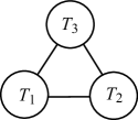
Figure 1: A typical structure of the theory realized on a system of giant gravitons. Each vertex represents the theory $T_{i}$ with rank $m_{i}$ realized on $m_{i}$ coincident giant gravitons wrapped around cycle $i$. Edges connecting vertices are degrees of freedom arising on intersections of cycles. $d=3$ case is shown.

It is the direct product of theories $T_{i}$ realized on cycles $i=1,\ldots,d$ coupling to the degrees of freedom arising on their intersections. $F^{(T)}_{m_{1},\ldots,m_{k}}$ are $N$-independent, and the $N$-dependence appears only through the prefactor $x_{1}^{m_{1}N}\cdots x_{d}^{m_{d}N}$.

Similar expansion of the index is also proposed in [24] based on a complementary analysis on the gauge theory side, and such expansions were named “the giant graviton expansions”. See also [25]. In their analysis the correspondents for giant gravitons and fluctuations on them are baryon operators and their modifications, respectively. Although there are some technical subtleties about the relation between these expansions obtained on the two sides of the AdS/CFT correspondence they are expected to be essentially the same.

In this work we focus on the contribution of giant gravitons wrapped around a single cycle $i$. Let $F^{(T)}_{i,m_{i}}=F^{(T)}_{0,\ldots,m_{i},\ldots,0}$ be such contributions. It is essentially the index $I_{m_{i}}^{(T_{i})}$ of the theory $T_{i}$ realized on the worldvolume of $m_{i}$ coincident giant gravitons. More precisely, $F_{i,m}^{(T)}$ and $I_{m}^{(T_{i})}$ are related by a simple variable change of the fugacities as we will explain shortly. A purpose of this work is to study this relation in detail.

For concreteness let us consider the Schur index [26] of the ${\cal N}=4$ $U(N)$ SYM. Let $J_{1}$ and $J_{2}$ be the angular momenta and $R_{x}$, $R_{y}$, and $R_{z}$ be the $R$ charges. The Schur index is defined by

$$I_{N}^{(D3)}(x,y)=\mathop{\rm tr}\nolimits[(-1)^{F}q^{J_{1}}x^{R_{x}}y^{R_{y}}],\quad q=xy,$$ (2)

where we denote the ${\cal N}=4$ $U(N)$ SYM by $T=D3$. The constraint $q=xy$ is necessary to preserve the supersymmetry. We eliminate $q$ by the constraint and treat the index as a function of $x$ and $y$.

The giant graviton expansion for the Schur index is given in [17] as the double expansion

$$\frac{I_{N}^{(D3)}}{I^{(D3)}_{\infty}}=\sum_{m_{x}=0}^{\infty}\sum_{m_{y}=0}^{\infty}x^{m_{x}N}y^{m_{y}N}F^{(D3)}_{m_{x},m_{y}}.$$ (3)

The two non-negative integers $m_{x}$ and $m_{y}$ are wrapping numbers over the cycles $i=x$ and $i=y$, respectively, which are respectively defined to be the $R_{x}$ and $R_{y}$ fixed roci in $M_{D3}=S^{5}$. A special property of the Schur index is that the functions $F_{m_{x},m_{y}}^{(D3)}$ are factorized [17]:

$$F_{m_{x},m_{y}}^{(D3)}=(xy)^{m_{x}m_{y}}F^{(D3)}_{x,m_{x}}F^{(D3)}_{y,m_{y}}.$$ (4)

Therefore, we only need to determine $F_{i,m}^{(D3)}$ to write down the expansion (3). $F_{i,m}^{(D3)}$ is the index of the ${\cal N}=4$ $U(m)$ SYM realized on $m$ coincident giant gravitons wrapped around the cycle $i(=x,y)$. The theories $T$, $T_{x}$, and $T_{y}$ are accidentally the same in this case, and the corresponding indices $I_{N}^{(D3)}$, $F_{x,N}^{(D3)}$, and $F_{y,N}^{(D3)}$ are also essentially the same functions. Careful analysis of the action of superconformal algebra on the $AdS$ boundary and that on giant gravitons wrapped around the cycle $x$ shows that they are related by the involution [16]

$$(H,J_{1},J_{2},R_{x},R_{y},R_{z})\rightarrow(H-2R_{x},R_{y},R_{z},-R_{x},J_{1},J_{2}).$$ (5)

A similar relation also holds for cycle $y$. This means that $I_{N}^{(D3)}(x,y)$ and $F_{i,N}^{(D3)}(x,y)$ are related by the variable changes [16]

$$F_{x,N}^{(D3)}(x,y)=I_{N}^{(D3)}(x^{-1},xy),\quad F_{y,N}^{(D3)}(x,y)=I_{N}^{(D3)}(xy,y^{-1}).$$ (6)

See also [24] for a derivation of (6) on the gauge theory side.

Despite the simplicity of (6), it is not straightforward to calculate $F_{i,N}^{(D3)}$ from $I_{N}^{(D3)}$, and vice versa, because we usually do not have analytic form of the indices, and only series expansions are available. The variable changes relate different convergence regions of the functions, and it is a non-trivial problem to generate one from another. In this paper, we propose a simple prescription to obtain the functions $F_{i,N}^{(T)}$ from $I_{N}^{(T_{i})}$.

To understand the relation, we need to carefully analyze the dependence of the series expansion on the choice of expansion variables. Different choices of expansion variables give different series expansions. Indeed, the expansion found in [24] is the simple expansion over a single non-negative integer $m$:

$$\frac{I_{N}^{(T)}}{I_{\infty}^{(T)}}=\sum_{m=0}^{\infty}x^{mN}F_{i,m}^{(T)}.$$ (7)

This looks different from the multiple expansion (1). Once we have understood the relation between $I_{N}^{(T_{i})}$ and $F_{i,N}^{(T)}$, we can give a partial explanation to this difference.

In the process of confirming the relation (7) the analytic continuation has been necessarily done in [24] for functions appearing in (7) based on a pole structure commonly found in the functions. Our prescription is useful to clarify the pole structure and enable us to study the relations like (6) in a systematic way.

The paper is organized as follows.

In the next section we prepare tools used in the following sections. In particular, we define “a domain” specifying the expansion variables. We also define the plethystic exponential and the plethystic logarithm with emphasis on the dependence on domains. In section 3 we explain the necessity of the analytic continuation, and propose a simple prescription to realize it. We numerically test the proposed method in Section 4 for the maximally supersymmetric theories realized on D3, M5, and M2-branes. The last section is devoted to conclusions and discussion.

2 Plethystic exponential and plethystic logarithm

The calculation of the index $I$ of a free field theory usually starts from the analysis of single-particle states. The corresponding index is called the letter index. It is obtained by summing up the contributions from all one-particle states. If there are two fugacities $x$ and $y$ it is given by

$$i=\sum_{(n_{x},n_{y})\in R}c_{n_{x},n_{y}}x^{n_{x}}y^{n_{y}},$$ (8)

where $R$ is a certain region on the $2$-dimensional charge lattice specifying a set of monomials appearing in the expansion. We call such a region “a domain.” We usually adopt $R$ such that it covers all one-particle states. We call such a domain “a physical domain”. For the Schur index of $T=D3$ we can take

$$R_{0}=\{(n_{x},n_{y})|n_{x},n_{y}\geq 0\}\backslash(0,0)$$ (9)

as a physical domain. Later we will discuss other choices of $R$. We call the series associated with a domain $R$ the $R$-series. For a free field theory the series sums up into a simple rational function. For example, the letter index of the ${\cal N}=4$ $U(1)$ vector multiplet is [4]

$$i^{(D3)}_{1}=1-\frac{(1-x)(1-y)}{1-xy},$$ (10)

and that of the type IIB supergravity multiplet in $AdS_{5}\times S^{5}$, which is dual to the large $N$ SYM, is [4]

$$i^{(D3)}_{\infty}=\frac{1}{1-x}+\frac{1}{1-y}-\frac{1}{1-xy}-1.$$ (11)

By expanding these functions into terms appearing in the domain $R_{0}$ we can obtain the set of coefficients in (8). In the following we use the notation $i|_{R}$ when we want to emphasize that $i$ is given as an $R$-series. We graphically express a series by plotting the coefficients in the two-dimensional lattice as shown in Figure 2.

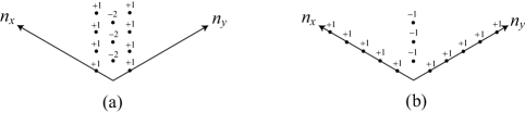
Figure 2: (a) The letter index $i_{1}^{(D3)}$ of the ${\cal N}=4$ vector multiplet. (b) The letter index $i_{\infty}^{(D3)}$ of the type IIB supergravity multiplet in $AdS_{5}\times S^{5}$.

Once we have obtained the letter index (8), the index for multi-particle states is uniquely determined by considering the combinatorics of the letters. The solution to this problem is

$$I=\mathop{\rm Pexp}\nolimits i,$$ (12)

where $\mathop{\rm Pexp}\nolimits$ is the plethystic exponential defined by

$$\mathop{\rm Pexp}\nolimits f(x,y)=\exp\left(\sum_{m=1}^{\infty}\frac{1}{m}f(x^{m},y^{m})\right).$$ (13)

For the definition (13) to make sense the condition $|x^{n_{x}}y^{n_{y}}|<1$ must hold for all terms appearing in the sum (8). This means all terms in $f$ must be contained in the domain $R_{(x,y)}$ defined by

$$R_{(x,y)}:=\{(n_{x},n_{y})|n_{x}\log|x|+n_{y}\log|y|<0\}.$$ (14)

For example, if we take $x$ and $y$ satisfying $|x|=|y|<1$, (14) gives the upper half plane with the horizontal boundary excluded, and all points of $i_{1}^{(D3)}$ and $i_{\infty}^{(D3)}$ shown in Figure 2 are contained in the domain. (Namely, we can use $R_{(x,y)}$ as a physical domain.) If $i$ is expanded with such a domain $R$, $I$ given by (12) can also be expanded in a similar form;

$$I=1+\sum_{(n_{x},n_{y})\in R}c^{\prime}_{n_{x},n_{y}}x^{n_{x}}y^{n_{y}}$$ (15)

with the same domain $R$. We can show that the map from $\{c_{n_{x},n_{y}}\}$ to $\{c^{\prime}_{n_{x},n_{y}}\}$ is one to one if

• $R$ is a sector with the center angle $\theta\leq\pi$.

• $R\cap(-R)=\phi$.

The latter is the condition for the boundary of $R$. We do not include the origin, and if $\theta=\pi$ we can include at most one of two boundary rays. We always require $R$ to satisfy these conditions, and then we can define the inverse operation to $\mathop{\rm Pexp}\nolimits$:

$$i=\mathop{\rm Plog}\nolimits I.$$ (16)

This is called the plethystic logarithm. It is important that we can introduce the group structure for $\mathop{\rm Pexp}\nolimits i$ under the multiplication, which corresponds to the addition for $i$.

Even for an interacting theory we can calculate the index by using localization method if it is a Lagrangian theory. For the ${\cal N}=4$ SYM with $U(N)$ gauge group the index is given by

$$I^{(D3)}_{N}|_{R_{(x,y)}}=\frac{1}{N!}\int\prod_{a=1}^{N}\frac{dz_{a}}{2\pi iz_{a}}\prod_{a\neq b}\left(1-\frac{z_{a}}{z_{b}}\right)\mathop{\rm Pexp}\nolimits\left(i_{1}^{(D3)}|_{R_{(x,y)}}\sum_{a,b}\frac{z_{a}}{z_{b}}\right),$$ (17)

where $z_{a}$ ($a=1,\ldots,N$) are gauge fugacities. As is explicitly shown we suppose $i_{1}^{(D3)}$ is given as an $R_{(x,y)}$-series. Usually $R_{(x,y)}$ is assumed to be a physical domain. This means that $|x^{n_{x}}y^{n_{y}}|<1$ is satisfied for all terms in $i_{1}^{(D3)}|_{R_{(x,y)}}$. If we take the unit circle $|z_{a}|=1$ for the integration contours $|x^{n_{x}}y^{n_{y}}\frac{z_{a}}{z_{b}}|<1$ is also satisfied, and $\mathop{\rm Pexp}\nolimits$ in (17) makes sense. The contour integrals extract the contribution of gauge invariant states and give $I_{N}$ as an $R_{(x,y)}$-series.

3 Variable changes and analytic continuation

In the following we frequently use the variable changes in (6), and it is convenient to introduce $\sigma_{x}$ and $\sigma_{y}$ to represent these variable changes as follows.

$$\sigma_{x}(x,y,q)=(x^{-1},q,y),\quad\sigma_{y}(x,y,q)=(q,y^{-1},x).$$ (18)

If we use the triangular lattice to express the series expansion as in Figure 2, $\sigma_{x}$ and $\sigma_{y}$ are the reflections through the lines perpendicular to $n_{x}$ and $n_{y}$ axes, respectively. With the maps $\sigma_{i}$ ($i=x,y$) the relations in (6) are expressed in the simple form

$$F_{i,N}^{(D3)}=\sigma_{i}I_{N}^{(D3)}\quad(i=x,y).$$ (19)

We want to confirm that $F_{i,N}^{(D3)}$ given by (19) correctly reproduce $I_{N}^{(D3)}$ via (3). Let $R$ be a physical domain used for the expansion of $I_{N}^{(D3)}$. To confirm the relation (3) holds we need $F_{i,N}^{(D3)}|_{R}$. However, the variable change $\sigma_{i}$ transforms $I_{N}^{(D3)}|_{R}$ into $F_{i,N}^{(D3)}|_{\sigma_{i}R}$, where $\sigma_{i}R$ is the image of $R$ under the map $\sigma_{i}$. Therefore, to compare the left hand side and the right hand side of (3), we need to resum or analytically continue $F_{i,N}^{(D3)}|_{\sigma_{i}R}$ to $F_{i,N}^{(D3)}|_{R}$.

In general, if we have $i|_{R}$ for a domain $R$, it can also be regarded as $i|_{R^{\prime}}$ for another domain $R^{\prime}$ which contains $R$ as a subset. Therefore, it is convenient to define “a maximal domain” which cannot be enlarged any more. $R$ is a maximal domain if

$$R\cup(-R)\cup O=L,$$ (20)

where $O$ is the origin and $L$ is the whole plane. A maximal domain $R$ is a sector with center angle $\pi$, and only one of the boundary rays is included in $R$.

Let us suppose that $f|_{R^{\prime}}$ for a maximal domain $R^{\prime}$ is given and we want to obtain $(\mathop{\rm Pexp}\nolimits f)|_{R}$ for another maximal domain $R\neq R^{\prime}$. We divide $R^{\prime}$ into the following two parts.

$$R_{1}=R^{\prime}\backslash R,\quad R_{2}=R^{\prime}\cap R.$$ (21)

By definition, $R^{\prime}=R_{1}\cup R_{2}$ and $R=(-R_{1})\cup R_{2}$. Correspondingly, we divide $f$ into two parts $f_{1}$ and $f_{2}$ so that $f|_{R^{\prime}}=f_{1}|_{R_{1}}+f_{2}|_{R_{2}}$. The plethystic exponential of $f|_{R^{\prime}}$ is factorized into two factors:

$$\mathop{\rm Pexp}\nolimits f|_{R^{\prime}}=(\mathop{\rm Pexp}\nolimits f_{1}|_{R_{1}})(\mathop{\rm Pexp}\nolimits f_{2}|_{R_{2}}).$$ (22)

The factor $\mathop{\rm Pexp}\nolimits f_{2}|_{R_{2}}$ can be regarded as an $R$-series. What we need to do to obtain $(\mathop{\rm Pexp}\nolimits f)|_{R}$ is to rewrite the other factor $\mathop{\rm Pexp}\nolimits f_{1}|_{R_{1}}$ as a $(-R_{1})$-series. This can be done by using analytic continuation as follows. Let us suppose that $f_{1}$ is given by

$$f_{1}(x,y)=\sum_{(n_{x},n_{y})\in R_{1}}c_{n_{x},n_{y}}x^{n_{x}}y^{n_{y}}.$$ (23)

For values of $x$ and $y$ such that $R_{1}\subset R_{(x,y)}$ we can rewrite the plethystic exponential in the product form

$$\mathop{\rm Pexp}\nolimits f_{1}|_{R_{1}}=\prod_{(n_{x},n_{y})\in R_{1}}\frac{1}{(1-x^{n_{x}}y^{n_{y}})^{c_{n_{x},n_{y}}}}.$$ (24)

Once we have obtained this expression, we can analytically continue this function to values of $x$ and $y$ such that $-R_{1}\subset R_{(x,y)}$. Then, we can rewrite (24) as

$$\prod_{(n_{x},n_{y})\in R_{1}}\frac{(-x^{n_{x}}y^{n_{y}})^{-c_{n_{x},n_{y}}}}{(1-x^{-n_{x}}y^{-n_{y}})^{c_{n_{x},n_{y}}}}=P(x,y)\mathop{\rm Pexp}\nolimits f_{1}(x^{-1},y^{-1})|_{-R_{1}},$$ (25)

where $P(x,y)$ is the monomial function

$$P(x,y)=\prod_{(n_{x},n_{y})\in R_{1}}(-x^{n_{x}}y^{n_{y}})^{-c_{n_{x},n_{y}}}.$$ (26)

It is important that if $f_{1}$ has infinitely many terms (26) may not be well-defined, and then our prescription does not work.

By combining (25) with the factor $\mathop{\rm Pexp}\nolimits f_{2}$ we obtain the analytically continued plethystic exponential associated with the domain $R$:

$$\mathop{\rm Pexp}\nolimits_{R}f\equiv P\mathop{\rm Pexp}\nolimits f^{\rm mod}|_{R}$$ (27)

where $f^{\rm mod}$ is defined by

$$f^{\rm mod}(x,y)=f_{1}(x^{-1},y^{-1})+f_{2}(x,y).$$ (28)

Each point $(n_{x},n_{y})\in R_{1}$ in $f$ is moved to the opposite point $(-n_{x},-n_{y})\in-R_{1}$ in the modified function $f^{\rm mod}$, and all terms of $f^{\rm mod}$ are contained in $R$.

In fact, essentially the same prescription has been used in previous works. Because giant gravitons are wrapped around topologically trivial cycles, there are unwrapping modes with negative excitation energies. Such modes are handled in [16, 17, 18] by applying the prescription explained above to the integrand of the gauge fugacity integrals. The variable change of the index after the gauge fugacity integrals has also been considered in [24]. Although detailed explanation is not given, the pole structure caused by the factor (24) was pointed out, and essentially the same method seems to be used.

The prescription explained above can be summarized in the following equations.

$$F_{i,N}^{(T)}|_{R}=\mathop{\rm Pexp}\nolimits_{R}\sigma_{i}i_{N}^{(T_{i})},\quad i_{N}^{(T_{i})}=\mathop{\rm Plog}\nolimits I_{N}^{(T_{i})}.$$ (29)

We first calculate $i_{N}^{(T)}$ as the plethystic logarithm of $I_{N}^{(T_{i})}$, and then we calculate the analytically continued plethystic exponential.

Unfortunately, it will turn out that this prescription works only in limited cases. If $\sigma_{i}i_{N}^{(T_{i})}$ has infinitely many points outside the domain $R$, then the factor (26) becomes an infinite product which in general does not converge. Even so, we will find that (29) is quite effective for simple expansion (7).

4 Numerical tests

In this section we numerically calculate $F_{i,N}^{(T)}$ from $I_{N}^{(T_{i})}$ by (29) in some examples and confirm the consistency with known results. The main results in 4.2 and 4.3 have been already given in [24].

4.1 Double expansion of the Schur index for $T=D3$

We first consider the double giant graviton expansion of the Schur index of $T=D3$ studied in [17]. Let us define ${\mathfrak{q}}$ and $u$ by

$$x={\mathfrak{q}}u,\quad y={\mathfrak{q}}u^{-1},\quad q={\mathfrak{q}}^{2}.$$ (30)

In [17] functions $F_{i,N}^{(D3)}$ are treated as ${\mathfrak{q}}$-series and the coefficients are given as rational functions of $u$. Here we do the further $u^{-1}$ expansion ($u$ expansion around $u=\infty$) after the ${\mathfrak{q}}$-expansion. This corresponds to the maximal physical domain (Figure 3 (a))

$$R_{qu} =\lim_{{\mathfrak{q}}\rightarrow 0,|u|>1}R_{(x,y)}$$

$$=\{(n_{x},n_{y})|n_{x}+n_{y}>0\}\cup\{(n_{x},n_{y})|n_{x}+n_{y}=0,n_{y}>0\}.$$ (31)

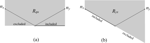
Figure 3: The maximal domains $R_{qu}$ and $R_{yx}$

Let us first consider $F_{x,1}^{(D3)}=\mathop{\rm Pexp}\nolimits(\sigma_{x}i_{1}^{(D3)})$ and $F_{y,1}^{(D3)}=\mathop{\rm Pexp}\nolimits(\sigma_{y}i_{1}^{(D3)})$. We find $\sigma_{x}i_{1}^{(D3)}$ has one term $x^{-1}={\mathfrak{q}}^{-1}u^{-1}$ that is not contained in $R_{qu}$, and we have to move it to the opposite point to define the modified letter index. For $\sigma_{y}i_{1}^{(D3)}$ we need to move two points corresponding to $xy^{-1}=u^{2}$ and $y^{-1}={\mathfrak{q}}^{-1}u$. See Figure 4.

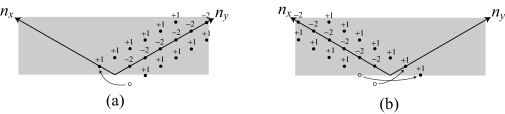
Figure 4: The modification of letter indices $\sigma_{x}i_{1}^{(D3)}$ and $\sigma_{y}i_{1}^{(D3)}$

Following the prescription explained in the previous section, we can calculate $F_{x,1}^{(D3)}|_{R_{qu}}$ and $F_{y,1}^{(D3)}|_{R_{qu}}$. The results are shown in Figure 5.

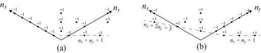
Figure 5: (a) $F_{x,1}^{(D3)}|_{R_{qu}}$ (b) $F_{y,1}^{(D3)}|_{R_{qu}}$

These agree with the results in [17]:

$$F_{x,1}^{(D3)} =(-u-u^{-1}-u^{-3}-\cdots){\mathfrak{q}}$$

$$+(-u^{2}+1){\mathfrak{q}}^{2}+(-u^{3}+u^{-3}){\mathfrak{q}}^{3}+(-u^{4}+1-u^{-2}+u^{-6}){\mathfrak{q}}^{4}+\cdots,$$

$$F^{(D3)}_{y,1} =(u^{-3}+u^{-5}+u^{-7}+\cdots){\mathfrak{q}}$$

$$+(1-u^{-2}){\mathfrak{q}}^{2}+(u^{3}-u^{-3}){\mathfrak{q}}^{3}+(u^{6}-u^{2}+1-u^{-4}){\mathfrak{q}}^{4}+\cdots.$$ (32)

This is not surprising because essentially the same prescription is used in [17] for the single giant graviton sector.

Next, let us apply (29) to $F_{i,N}^{(D3)}$ with $N\geq 2$. We first calculate $I_{N}^{(D3)}$ by (17), and calculate their plethystic logarithms $i_{N}^{(D3)}=\mathop{\rm Plog}\nolimits I_{N}^{(D3)}$. $i_{N}^{(D3)}$ have information not only about letters generating the operator spectra but also about non-trivial constraints among letters called “syzygies” [27]. The results for $N=2,3,4$ are shown in Figure 6.

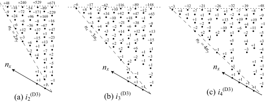
Figure 6: $i_{N}^{(D3)}$ for $N=2,3,4$ are shown. The distributions are left-right symmetric, and we show only the left half ($n_{x}\geq n_{y}$) of each plot. The dotted lines show a numerical cut-off $n_{x}+n_{y}\leq 20$.

The asymptotic behavior of the distribution of dots is important for the following analysis. We find in the plots in Figure 6 that except for finite number of dots near the origin almost all dots are contained in the sectors bounded by $E_{1}:n_{y}=Nn_{x}$ and $E_{2}:n_{x}=Nn_{y}$.

For $N=2$ the image of $E_{2}$ under $\sigma_{x}$, $\sigma_{x}E_{2}$, coincides with the right half of the horizontal line, which is the boundary of $R_{qu}$ (Figure 7).

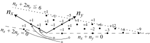
Figure 7: The modification of $\sigma_{x}i_{2}^{(D3)}$ for $R_{qu}$. The dotted line shows a numerical cut-off.

There are three points outside $R_{qu}$ corresponding to terms $x^{-1}={\mathfrak{q}}^{-1}u$, $x^{-2}={\mathfrak{q}}^{-2}u^{2}$, and $x^{-2}y={\mathfrak{q}}^{-1}u^{3}$. These give the factor $P=-{\mathfrak{q}}^{4}u^{-6}=-x^{5}y^{-1}$, and the analytically continued plethystic exponential is shown in Figure 8.

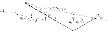
Figure 8: $F_{x,2}^{(D3)}|_{R_{qu}}$ is shown. The dotted line shows a numerical cut-off.

Again, we find agreement with the corresponding result in [17]:

$$F_{x,2}^{(D3)} =(-u^{6}+u^{4}+2+u^{-2}+3u^{-4}+2u^{-6}+\cdots){\mathfrak{q}}^{4}$$

$$+(-u^{9}+2u^{5}){\mathfrak{q}}^{5}+(-u^{12}+2u^{6}+2){\mathfrak{q}}^{6}+\cdots.$$ (33)

Next, let us consider $F_{y,2}^{(D3)}$. This time, $\sigma_{y}E_{1}$ is the semi-infinite horizontal line, and unlike the previous case the line is not contained in $R_{qu}$. This means that there are infinitely many points outside $R_{qu}$, and the factor (26) becomes infinite product. Therefore, (29) does not work. In fact, this is also expected from $F_{y,2}^{(D3)}$ in [17]:

$$F_{y,2}^{(D3)}({\mathfrak{q}},u) =(2u^{-10}+u^{-12}+3u^{-14}+\cdots){\mathfrak{q}}^{4}+\cdots.$$ (34)

As we see, the leading term has coefficient $2$, and it is impossible to obtain such a series by the plethystic exponential.

For $N=3$ and $4$ the situation is worse. Both $\sigma_{x}$ and $\sigma_{y}$ maps one of $E_{1}$ and $E_{2}$ below the boundary of $R_{qu}$, and there are infinitely many points outside $R_{qu}$, which make the factor (26) ill-defined. We can also see that the leading term coefficients of the functions in [17] are not $\pm 1$.

$$F_{x,3}^{(D3)} =(-2u^{15}+u^{13}+\cdots){\mathfrak{q}}^{9}+\cdots,$$

$$F_{y,3}^{(D3)} =(5u^{-21}+2u^{-23}+\cdots){\mathfrak{q}}^{9}+\cdots,$$

$$F_{x,4}^{(D3)} =(-5u^{28}+2u^{26}+\cdots){\mathfrak{q}}^{16}+\cdots,$$

$$F_{y,4}^{(D3)} =(14u^{-36}+5u^{-38}+\cdots){\mathfrak{q}}^{16}+\cdots.$$ (35)

These expansions cannot be reproduced by the relation (29).

4.2 Simple expansion of the Schur index for $T=D3$

Let us consider the simple giant graviton expansion investigated in [24]. The index is treated in [24] as a series obtained by the successive expansions in which $y$ expansion is carried out first and then $x$ expansion is done for the coefficients of the first expansion. The associated maximal physical domain is (Figure 3 (b))

$$R_{yx}=\lim_{y\rightarrow 0,|x|<1}R_{(x,y)}=\{(n_{x},n_{y})|n_{y}>0\}\cup\{(n_{x},0)|n_{x}>0\}.$$ (36)

Let us start with the analysis of $F_{x,1}^{(D3)}|_{R_{yx}}$ and $F_{y,1}^{(D3)}|_{R_{yx}}$.

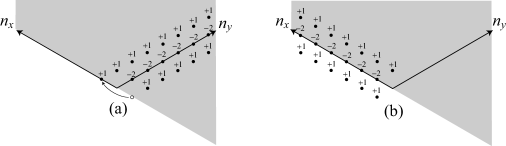
Figure 9: (a) The modification of $\sigma_{x}i_{1}$. (b) $\sigma_{y}i_{1}$

For $\sigma_{x}i_{1}^{(D3)}$, there is one dot outside $R_{yx}$ (Figure 9 (a)). This is the same as in Figure 4 (a), and hence we obtain the same result for $F_{x,1}^{(D3)}$ as the previous subsection (Figure 5 (a)). However, for $\sigma_{y}i_{1}^{(D3)}$, there are infinitely many points outside $R_{yx}$ corresponding to terms $y^{-1}x^{k}$ ($k=0,1,2,\ldots$) (Figure 9 (b)), and (26) becomes

$$P=\prod_{k=0}^{\infty}(-yx^{-k}).$$ (37)

Although this is an infinite product, we can give it significance. $P$ includes the factor $y^{+\infty}$, and the contribution decouples. We can simply treat $F_{y,1}^{(D3)}|_{R_{yx}}$ as $0$. Namely, as far as single-wrapping giant graviton contributions are concerned, the difference between the multiple expansion (1) and the simple expansion (7) comes from the different choice of the domains.

Let us proceed to $N\geq 2$ contributions. For $\sigma_{y}i_{N}^{(D3)}$, we find infinitely many points outside $R_{qu}$, just like the $N=1$ case. Because both positive and negative coefficients appear, it is not clear whether they decouple like $F_{y,1}^{(D3)}$. Here, based on the analysis in [24], we simply assume their decoupling and focus only on $F_{x,N}^{(D3)}$.

In $i_{N}^{(D3)}$ shown in Figure 6 we find $N$ dots on the positive part of the $n_{x}$ axis corresponding to the $1/2$ BPS operators $\mathop{\rm tr}\nolimits X^{k}$ ($k=1,2,\ldots,N$). By $\sigma_{x}$ they are mapped to the $N$ points on the negative part of the $n_{x}$ axis. Because they are not contained in $R_{yx}$ we need to move them back to the opposite points on the positive part of the $n_{x}$ axis (Figure 10).

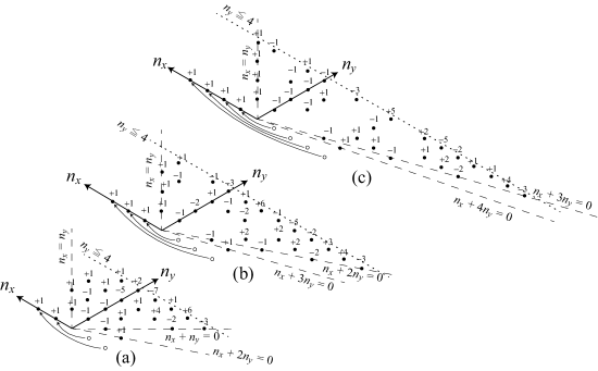
Figure 10: The modification of $i_{N}^{(D3)}$ for $R_{yx}$ for $N=2,3,4$. (a) $\sigma_{x}i_{2}$. (b) $\sigma_{x}i_{3}$. (c) $\sigma_{x}i_{4}$. The dotted lines show a numerical cut-off

The factorization corresponding to (22) is

$$I_{N}^{(D3)}(x,y)=\frac{1}{\prod_{k=1}^{N}(1-x^{k})}I^{\prime(D3)}_{N}(x,y),$$ (38)

The fractional factor coming from the $N$ points on the $n_{x}$ axis and produces poles on the $x$-plane at $k$-roots of unity with $1\leq k\leq N$. As is pointed out in [24] these are only poles we need to take care of in the analytic continuation. The function $I^{\prime(D3)}_{N}$ corresponds to all other points with $n_{y}\geq 1$ in the range $0\leq n_{x}\leq(N+1)n_{y}$. The coefficient of $y$-expansion $I^{\prime(D3)}_{N}$ at order $n_{y}$ is a Laurant polynomial of $x$ consisting of terms in this range. Therefore, we can safely perform the variable change $\sigma_{x}$ for the function $I^{\prime(D3)}_{N}$. After the variable change we obtain

$$F_{x,N}^{(D3)}=\frac{(-1)^{N}x^{\frac{N(N+1)}{2}}}{\prod_{k=1}^{N}(1-x^{k})}\sigma_{x}I^{\prime(D3)}_{N}$$ (39)

where $\sigma_{x}I^{\prime(D3)}_{N}$ has terms in the range $-Nn_{y}\leq n_{x}\leq n_{y}$ for each order of its $y$-expansion. Including the fractional factor with the numerator $(-1)^{N}x^{\frac{N(N+1)}{2}}$, we obtain $F_{x,N}^{(D3)}|_{R_{yx}}$ consisting of terms in the region (Figure 11)

$$\frac{N(N+1)}{2}-Nn_{y}\leq n_{x}.$$ (40)

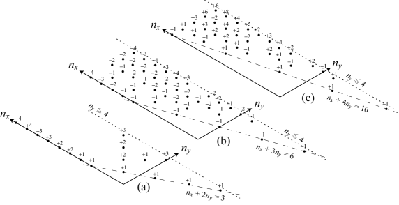
Figure 11: (a) $F_{x,2}^{(D3)}|_{R_{yx}}$. (b) $F_{x,3}^{(D3)}|_{R_{yx}}$. (c) $F_{x,4}^{(D3)}|_{R_{yx}}$. The dotted lines show a numerical cut-off.

As is confirmed in [24], the simple expansion (7) correctly reproduces the index $I_{N}^{(D3)}$ for different values of $N$. See Figure 12.

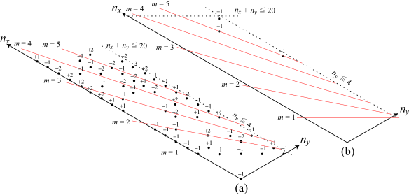
Figure 12: The result of numerical check for $N=3$. (a) The ratio $I_{3}^{(D3)}/I_{\infty}^{(D3)}$. (b) $(I_{3}^{(D3)}/I_{\infty}^{(D3)})-\sum_{m=0}^{4}x^{mN}F_{x,m}^{(D3)}$. The dotted lines show numerical cut-offs. The red lines labeled by $m$ show thresholds for respective wrapping numbers. Up to expected errors due to the $m=5$ contribution indicated by the line labeled by $m=5$, all terms are correctly canceled.

4.3 Superconformal index for $T=D3$

In the analysis of the Schur index we could focus on $F_{i,N}^{(D3)}|_{R}$ thanks to the factorization (4). This is not the case for the superconformal index without the Schur limit taken. The superconformal index of the ${\cal N}=4$ SYM is defined by [4]

$$I^{(D3)}=\mathop{\rm tr}\nolimits[(-1)^{F}q^{J_{1}}p^{J_{2}}x^{R_{x}}y^{R_{y}}z^{R_{z}}],\quad qp=xyz.$$ (41)

The giant graviton expansion investigated in [18] is a triple expansion with functions $F_{m_{x},m_{y},m_{z}}^{(D3)}$ in the summand, and the involution (5) gives the following relation between $F_{x,N}^{(D3)}=F_{N,0,0}^{(D3)}$ and $I_{N}^{(D3)}$ [16, 24]:

$$F_{x,N}^{(D3)}(p,q,x,y,z)=I_{N}^{(D3)}(y,z,x^{-1},p,q).$$ (42)

Let $\sigma_{x}$ denote this variable change. $F_{0,N,0}^{(D3)}$ and $F_{0,0,N}^{(D3)}$ are also related to $I_{N}^{(D3a)}$ via similar variable changes, which we denote by $\sigma_{y}$ and $\sigma_{z}$, respectively.

Due to the absence of the factorization, we need to calculate functions $F_{m_{x},m_{y},m_{z}}^{(D3)}$ directly by using localization formula similar to (17). The letter index appearing in the integrand of the localization formula contains $\sigma_{x}i_{1}^{(D3)}$, $\sigma_{y}i_{1}^{(D3)}$, and $\sigma_{z}i_{1}^{(D3)}$ at the same time, where $i_{1}^{(D3)}$ is given by [4]

$$i_{1}^{(D3)}=1-\frac{(1-x)(1-y)(1-z)}{(1-q)(1-p)}.$$ (43)

Even if we use a maximal domain we cannot cover three functions $\sigma_{i}i_{1}^{(D3)}$ with a single domain, and we need to use deformed contours for the gauge fugacity integrals [18, 25].

Despite the absence of the factorization, the analysis in [24] suggests that only $F_{x,m}^{(D3)}$ contribute to the index if we use an appropriate domain, and then our relation (29) is still useful to obtain $F_{x,N}^{(D3)}$ from $I_{N}^{(D3)}$. Corresponding to four independent variables we need to use a four-dimensional lattice to express full expansion of the index. To make two-dimensional plot possible we project the four-dimensional lattice onto the two-dimensional lattice corresponding to the unrefinement $y=z$ and $p=q$. Then, the index becomes function of $x$ and $y$ just like the Schur index. The letter indices $i_{1}^{(D3)}$ and $\sigma_{i}i_{1}^{(D3)}$ ($i=x,y,z$) after the projection are shown in Figure 13.

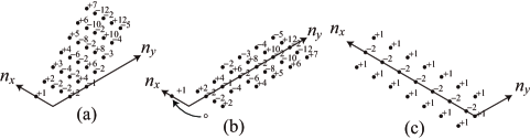
Figure 13: (a) The letter index $i_{1}^{(D3)}$ (b) The modification of $\sigma_{x}i_{1}^{(D3)}$ for $R_{yx}$. (c) $\sigma_{y}i_{2}^{(D3)}$ and $\sigma_{z}i_{2}^{(D3)}$ are identical after the projection to the two-dimensional lattice.

We see that if we use the domain $R_{yx}$ $F_{y,1}^{(D3)}$ and $F_{z,1}^{(D3)}$ decouple just like the Schur index, and $F_{x,1}^{(D3)}$ is the only contribution with $m_{x}+m_{y}+m_{z}=1$. Although we cannot prove the decoupling of all $F_{m_{x},m_{y},m_{z}}^{(D3)}$ with $m_{y}+m_{z}\geq 1$, the analysis in [24] shows that we can reproduce the finite $N$ index by the simple expansion containing only $F_{x,m}^{(D3)}$. See Figure 14 for the result of a numerical test.

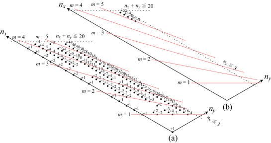
Figure 14: (a) The ratio of the superconformal indices $I_{N}^{(D3)}/I_{\infty}^{(D3)}$ for $N=3$. (b) $(I_{N}^{(D3)}/I_{\infty}^{(D3)})-\sum_{m=0}^{4}x^{mN}F_{x,N}^{(D3)}$ for $N=3$. The dotted lines show numerical cut-offs. The red lines labeled by $m$ show thresholds for respective wrapping numbers. Only small number of dots, which are consistent with the higher order contributions with $m\geq 5$, are left.

4.4 M5 from M2

Let us apply our method to the theory realized on $N$ coincident M5-branes, which we denote by $T=M5$. It is the $6$-dim ${\cal N}=(2,0)$ theory of $A_{N-1}$ type together with a free tensor multiplet.

The superconformal index is defined by [28]

$$I_{N}^{(M5)}=\mathop{\rm tr}\nolimits[(-1)^{F}\check{q}_{1}^{\check{J}_{12}}\check{q}_{2}^{\check{J}_{34}}\check{q}_{3}^{\check{J}_{56}}\check{x}_{1}^{\check{R}_{12}}\check{x}_{2}^{\check{R}_{34}}]\quad\check{q}_{1}\check{q}_{2}\check{q}_{3}=\check{x}_{1}\check{x}_{2},$$ (44)

where $\check{J}_{12}$, $\check{J}_{34}$, and $\check{J}_{56}$ are Cartan generators of $SO(6)_{\rm spin}$ and $\check{R}_{12}$ and $\check{R}_{34}$ are Cartan generators of $SO(5)_{R}$.

The index is given as a double giant graviton expansion associated with two two-cycles in [21], and the single giant graviton sector has been studied. The cycles are defined as the fixed loci of $\check{R}_{12}$ and $\check{R}_{34}$ in $M_{M5}=S^{4}$. We call $\check{R}_{12}$ ($\check{R}_{34}$) fixed locus “12-cycle” (“34-cycle”). M2-branes wrapped around these cycles contribute to the index.

The superconformal index of the $3$d ${\cal N}=8$ SCFT realized on coincident M2-branes is defined by [28]

$$I_{N}^{(M2)}=\mathop{\rm tr}\nolimits[(-1)^{F}\hat{q}^{\hat{J}_{12}}\hat{x}_{1}^{\hat{R}_{12}}\hat{x}_{2}^{\hat{R}_{34}}\hat{x}_{3}^{\hat{R}_{56}}\hat{x}_{4}^{\hat{R}_{78}}]\quad\hat{q}=\hat{x}_{1}\hat{x}_{2}\hat{x}_{3}\hat{x}_{4},$$ (45)

where $\hat{J}_{12}$ is the spin and $\hat{R}_{12}$, $\hat{R}_{34}$, $\hat{R}_{56}$, and $\hat{R}_{78}$ are $SO(8)_{R}$ Cartan generators. We can calculate this index for an arbitrary $N$ by applying the localization method [29] to the ABJM theory with Chern-Simons level $k=1$ [30].

The Cartan generators of the $3$d ${\cal N}=8$ superconformal algebra acting on M2-branes wrapped around $12$-cycle and those of the $6$d ${\cal N}=(2,0)$ superconformal algebra acting on the $AdS_{7}$ boundary are related by [21]

$$(\hat{H},\hat{J}_{12},\hat{R}_{12},\hat{R}_{34},\hat{R}_{56},\hat{R}_{78})=(\tfrac{1}{2}\check{H}-\tfrac{3}{2}\check{R}_{12},\check{R}_{34},\check{J}_{12},\check{J}_{34},\check{J}_{56},-\check{R}_{12}).$$ (46)

Correspondingly, the fugacities in (44) and those in (45) are related by

$$\sigma_{12}(\hat{q},\hat{x}_{1},\hat{x}_{2},\hat{x}_{3},\hat{x}_{4})=(\check{x}_{2},\check{q}_{1},\check{q}_{2},\check{q}_{3},\check{x}_{1}^{-1}).$$ (47)

The variable change associated with $34$-cycle, $\sigma_{34}$, is given by swapping $\check{x}_{1}$ and $\check{x}_{2}$ after $\sigma_{12}$. the M2-giant contributions $F_{12,N}^{(M5)}$ are obtained from the index $I_{N}^{(M2)}$ by the relation

$$F_{12,N}^{(M5)}=\sigma_{12}I_{N}^{(M2)}.$$ (48)

Again, there are four independent variables and the lattice is four-dimensional. We want to define a projection to two-dimensional lattice to show an expansion as a two-dimensional plot. We introduce variables $x$, $y$, and $u_{i}$ ($i=1,2,3$) by

$$\check{q}_{i}=yu_{i}\quad(u_{1}u_{2}u_{3}=1),\quad\check{x}_{1}=x,\quad\check{x}_{2}=x^{-1}y^{3}.$$ (49)

We focus on $x$ and $y$ to show series in figures.

We also rewrite the fugacities for M2-branes as follows:

$$\hat{q}=xy^{3},\quad\hat{x}_{i}=yu_{i}\quad(u_{1}u_{2}u_{3}=1),\quad\hat{x}_{4}=x.$$ (50)

Then, the variable change (47) becomes

$$\sigma_{12}(x,y,u_{i})=(x^{-1},y,u_{i}).$$ (51)

Namely, (48) becomes

$$F_{12,N}^{(M5)}(x,y,u_{i})=I_{N}^{(M2)}(x^{-1},y,u_{i}).$$ (52)

As in the previous examples, let us first look at the letter index for a single giant graviton. The theory on a single M2-brane is the free theory of an ${\cal N}=8$ scalar multiplet with the letter index [28]

$$i_{1}^{(M2)}=\frac{\hat{x}_{1}+\hat{x}_{2}+\hat{x}_{3}+\hat{x}_{4}-\hat{q}(\hat{x}_{1}^{-1}+\hat{x}_{2}^{-1}+\hat{x}_{3}^{-1}+\hat{x}_{4}^{-1})}{1-\hat{q}}.$$ (53)

We show $i_{1}^{(M2)}$, $\sigma_{12}i_{1}^{(M2)}$, and $\sigma_{34}i_{1}^{(M2)}$ projected on the two-dimensional plane in Figure 15.

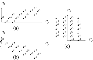
Figure 15: (a) The letter index $i_{1}^{(M2)}$. (b) The modification of $\sigma_{1}i_{1}^{(M2)}$ for $R_{yx}$. (c) Infinitely many dots of $\sigma_{2}i_{1}^{(M2)}$ are out of $R_{yx}$.

If we take the domain $R_{yx}$ defined in (36), $\sigma_{34}i_{1}^{(M2)}$ has infinitely many points outside $R_{yx}$. They give the factor

$$P=\prod_{k=1}^{\infty}(-y^{3}x^{-k})\prod_{k=1}^{\infty}(-yx^{-k})^{-3}.$$ (54)

If we take the product for each $k$ first, we obtain $\prod_{k=1}^{\infty}x^{2k}=x^{\infty}$ and the contribution decouples. Just like the previous examples, we simply assume that $F_{m_{12},m_{34}}^{(M5)}$ with $m_{34}\geq 1$ decouple, and let us consider the simple expansion associated with the $12$-cycle

$$\frac{I_{N}^{(M5)}}{I_{\infty}^{(M5)}}=\sum_{m=0}^{\infty}x^{mN}F_{12,m}^{(M5)}.$$ (55)

Let us numerically confirm (55) holds for small $N$. $I_{N}^{(M5)}$ with $N=-1,0,1$ and $\infty$ are given by

$$I_{-1}^{(M5)}=0,\quad I_{0}^{(M5)}=1,\quad I_{1}^{(M5)}=\mathop{\rm Pexp}\nolimits i_{1}^{(M5)},\quad I_{\infty}^{(M5)}=\mathop{\rm Pexp}\nolimits i_{\infty}^{(M5)},$$ (56)

where $i_{1}^{(M5)}$ and $i_{\infty}^{(M5)}$ are the letter indices of the tensor multiplet and the supergravity multiplet in $AdS_{7}\times S^{4}$. They are given by [28]

$$i_{1}^{(M5)}=\frac{\check{x}_{1}+\check{x}_{2}-\check{q}_{1}\check{q}_{2}-\check{q}_{2}\check{q}_{3}-\check{q}_{3}\check{q}_{1}+\check{x}_{1}\check{x}_{2}}{(1-\check{q}_{1})(1-\check{q}_{2})(1-\check{q}_{3})},$$ (57)

and

$$i_{\infty}^{(M5)}=\frac{\check{x}_{1}+\check{x}_{2}-\check{q}_{1}\check{q}_{2}-\check{q}_{2}\check{q}_{3}-\check{q}_{3}\check{q}_{1}+\check{x}_{1}\check{x}_{2}(\check{q}_{1}+\check{q}_{2}+\check{q}_{3}-\check{x}_{1}-\check{x}_{2})}{(1-\check{x}_{1})(1-\check{x}_{2})(1-\check{q}_{1})(1-\check{q}_{2})(1-\check{q}_{3})}.$$ (58)

By using these we can calculate the left hand side of (55). In the following we calculate the right hand side of (55).

We first calculate the index $I_{N}^{(M2)}$ for different $N$ with the physical domain $R_{yx}$. This is done by applying localization method [29] to the ABJM theory [30]. The plethystic logarithms $i_{N}^{(M2)}$ for small $N$ are shown in Figure 16.

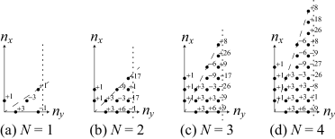
Figure 16: $i_{N}^{(M2)}=\mathop{\rm Plog}\nolimits I_{N}^{(M2)}$ for $N=1,2,3,4$ are shown. As shown by the dotted lines the $y$ expansions are cut off at $n_{y}=3$.

They have similar structure to $i_{N}^{(D3)}$. In particular, for each $N$ there are $N$ dots on the positive part of the vertical axis corresponding to $N$ $1/2$ BPS operators. After the variable change (51), these dots have to be moved to the opposite points to obtain the modified letter index. The expansion of the analytically continued plethystic exponential $F_{12,N}^{(M5)}|_{R_{yx}}=\mathop{\rm Pexp}\nolimits_{R_{yx}}\sigma_{12}i_{N}^{(M2)}$ for $N=1,2,3,4$ are shown in Figure 17.

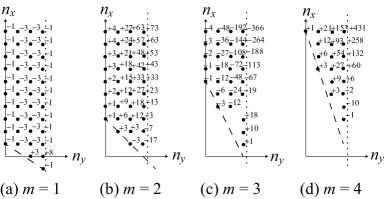
Figure 17: M2-giant contributions $F_{12,m}^{(M5)}$ with wrapping number $m=1,2,3,4$ are shown. As shown by the dotted lines the $y$ expansions are cut off at $n_{y}=3$.

For $N\geq 2$ the dots are in the region above the line $n_{x}=\frac{m(m+1)}{2}+mN-mn_{y}$. ($N=1$ case is exceptional and the line is $n_{x}=1-\frac{2}{3}n_{y}$.)

With the functions $F_{12,m}^{(M5)}$ obtained above we can confirm that (55) holds for $N=-1,0,1$ up to expected errors. See Figure 18.

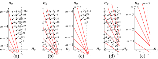
Figure 18: The results of consistency check for $N=-1,0,1$. $I_{N}^{(M5)}/I_{\infty}^{(M5)}$ for $N=0$ and $N=1$ are shown in (b) and (d), respectively. Trivial one, $I_{-1}^{(M5)}/I_{\infty}^{(M5)}=0$ is not shown. $(I_{N}^{(M5)}/I_{\infty}^{(M5)})-\sum_{m=0}^{4}x^{mN}F_{12,m}^{(M5)}$ for $N=-1$, $0$, and $1$ are shown in (a), (c), and (e),respectively. As shown by the dotted lines the $y$ expansions are cut off at $n_{y}=3$. In (a), (c), and (e), all terms below the $m=5$ lines are correctly canceled, and only expected errors due to $m\geq 5$ contributions are left.

This strongly suggests that (55) correctly gives $I_{N}^{(M5)}$ for an arbitrary $N$. Although we only show the two-dimensional plots, we can calculate the full superconformal index. See Appendix A.

We can also compare our results with the analytic result for the Schur-like limit [31, 32] obtained from the analysis of five-dimensional SYM. It is known that by setting $\check{q}_{1}=\check{x}_{1}$, the index $I_{N}^{(M5)}$ reduces to the following function of the single variable $\check{x}_{1}$:

$$I_{N}^{(M5)}=\mathop{\rm Pexp}\nolimits\frac{\check{x}_{1}+\check{x}_{1}^{2}+\cdots+\check{x}_{1}^{N}}{1-\check{x}_{1}}.$$ (59)

If we take the same limit in our results shown in Appendix A we obtain

$$I_{2}^{(M5)} =1+\check{x}_{1}+3\check{x}_{1}^{2}+5\check{x}_{1}^{3}+10\check{x}_{1}^{4}+\underline{15\check{x}_{1}^{5}}+{\cal O}(\check{x}_{1}^{6}),$$

$$I_{3}^{(M5)} =1+\check{x}_{1}+3\check{x}_{1}^{2}+6\check{x}_{1}^{3}+12\check{x}_{1}^{4}+\underline{20\check{x}_{1}^{5}}+{\cal O}(\check{x}_{1}^{6}),$$

$$I_{4}^{(M5)} =1+\check{x}_{1}+3\check{x}_{1}^{2}+6\check{x}_{1}^{3}+13\check{x}_{1}^{4}+\underline{22\check{x}_{1}^{5}}+{\cal O}(\check{x}_{1}^{6}),$$

$$I_{5}^{(M5)} =1+\check{x}_{1}+3\check{x}_{1}^{2}+6\check{x}_{1}^{3}+13\check{x}_{1}^{4}+\underline{23\check{x}_{1}^{5}}+{\cal O}(\check{x}_{1}^{6}).$$ (60)

We only showed terms independent of $\check{q}_{2}$ and $\check{q}_{3}$. The underlines indicate the terms are incorrect. These are consistent with (59) because in our numerical results the $y$ expansion is cut off at $n_{y}=3$ and the expected order of errors is ${\cal O}(\check{x}_{1}^{4})$ or higher. The $\check{q}_{2}$ or $\check{q}_{3}$-dependent terms which we did not show in (60) are also consistent with the expected errors.

Note that the Schur-like limit is ill-defined for each M2-giant contribution because the limit corresponds to $\hat{x}_{1}=\hat{x}_{4}^{-1}$ via (47). The terms $\hat{x}_{1}$ and $\hat{x}_{1}^{-1}$ appear at the same time in the letter index $i_{1}^{(M2)}$ in the limit, and there is no domain covering both of them. We need to take the limit after summing up the contributions of M2-giants.

4.5 M2 from M5

It is possible to interchange the roles of M2 and M5 in the previous subsection. Namely, we can calculate the finite $N$ index of M2 theory by summing up M5-giant contributions by the relation

$$\frac{I_{N}^{(M2)}|_{R_{yx}}}{I_{\infty}^{(M2)}|_{R_{yx}}}=\sum_{m=0}^{\infty}x^{mN}(\sigma_{12}^{-1}I_{m}^{(M5)})|_{R_{yx}},$$ (61)

where the large $N$ index is given by $I_{\infty}^{(M2)}=\mathop{\rm Pexp}\nolimits i_{\infty}^{(M2)}$ with the letter index [28]

$$i_{\infty}^{(M2)}=\frac{(1-\hat{q}\hat{x}_{1}^{-1})(1-\hat{q}\hat{x}_{2}^{-1})(1-\hat{q}\hat{x}_{3}^{-1})(1-\hat{q}\hat{x}_{4}^{-1})}{(1-\hat{x}_{1})(1-\hat{x}_{2})(1-\hat{x}_{3})(1-\hat{x}_{4})(1-\hat{q})^{2}}-\frac{1-\hat{q}+\hat{q}^{2}}{(1-\hat{q})^{2}}.$$ (62)

The calculation to test (61) is parallel to the previous example, and we only give a brief explanation.

In [21] four five-cycles in $M_{M5}=S^{7}$ were taken into account. As the previous examples we can show for a single M5 giant that if we take $R_{yx}$ only one of the four cycles, $\hat{R}_{78}$ fixed locus, gives non-trivial contribution. Hence, we focus on $F_{78,N}^{(M2)}$ associated with the cycle.

By using the results of previous subsection for $I_{N}^{(M5)}$ we can obtain the plethystic logarithms $i_{N}^{(M5)}=\mathop{\rm Plog}\nolimits I_{N}^{(M5)}$ for small $N$ shown in Figure 19.

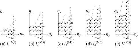
Figure 19: $i_{N}^{(M5)}$ for $N=1,2,3,4,5$ are shown. As shown by the dotted lines the $y$ expansions are cut off at $n_{y}=3$.

As the previous examples we find $N$ dots associated with the $1/2$ BPS operators on the positive part of the vertical axis for each $N$. The functions $F_{78,N}^{(M2)}=\mathop{\rm Pexp}\nolimits_{R_{yx}}\sigma_{12}^{-1}i_{N}^{(M5)}$ are shown in Figure 20.

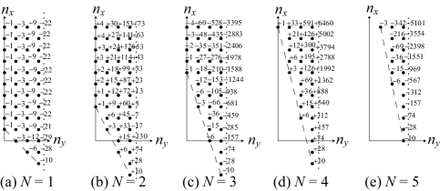
Figure 20: M5 giants contributions $F_{78,N}^{(M2)}$ for $N=1,2,3,4,5$ are shown. As shown by the dotted lines the $y$ expansions are cut off at $n_{y}=3$.

The results of a numerical check of (61) for $N=-1,0,1$ are shown in Figure 21.

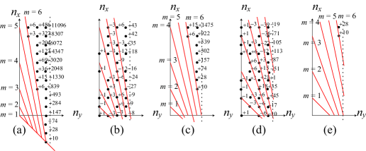
Figure 21: $(I_{N}^{(M2)}/I_{\infty}^{(M2)})$ for $N=0,1$ are shown in (b) and (d), respectively. The trivial one $I_{-1}^{(M2)}/I_{\infty}^{(M2)}=0$ is not shown. $(I_{N}^{(M2)}/I_{\infty}^{(M2)})-\sum_{m=0}^{5}x^{mN}F_{78,m}^{(M2)}$ for $N=-1,0,1$ are shown in (a), (c), and (e), respectively. As shown by the dotted lines the $y$ expansions are cut off at $n_{y}=3$. In (a), (c), and (e) all terms below $m=6$ lines are correctly canceled, and only expected errors due to $m\geq 6$ contributions are left.

5 Conclusions and Discussion

We investigated the giant graviton expansions. In particular, we concentrated on coincident giant gravitons wrapped around a single cycle. Because the expansion domain for giant gravitons and that of the boundary theory are different, we need to perform an analytic continuation to relate them. We proposed a simple prescription (29) to realize it.

We explicitly showed for the Schur index of $T=D3$ that different choices of the expansion domains give different functions for single giant graviton contributions $F_{i,1}^{(D3)}$ ($i=x,y$). If we use $R_{qu}$ in (31) both $F_{x,1}^{(D3)}$ and $F_{y,1}^{(D3)}$ contribute to the Schur index, while if we use $R_{yx}$ in (36), $F_{y,1}^{(D3)}$ does not contribute. Although we have not proved $F_{y,N\geq 2}^{(D3)}$ also vanish, this partially explains why there are two different expansions: the simple expansion found in [24] and the multiple expansion in [17]. It is surprising that they give the same result even though some contributions are lost in the simple expansion. This may be related to the fact that the set of functions $F_{m_{x},m_{y}}$ are strongly constrained. For example, we can formally substitute negative $N$ to expansion (1) or (7), and find that the result is vanishing. This gives very strong constraints on the functions. This implies that the functions share common information, and only small subset appearing in the simple expansion may be sufficient to give the complete answer. It would be interesting to investigate the structure of the constrained set of the functions.

An important application of our method is the calculation of the full superconformal index of the 6d ${\cal N}=(2,0)$ $A_{N-1}$ SCFT. It is in principle possible to calculate $I_{N}^{(M5)}$ for an arbitrary $N$ up to an arbitrary order starting from the indices $I_{m}^{(M2)}$ of the M2-brane theories with different $m$. Some results are shown in Appendix A.

An important merit of our method is that the theory on giant gravitons does not have to be Lagrangian theories unlike the method adopted in [17, 18, 25], which uses deformed contours in the gauge fugacity integrals to realize the analytic continuation. We only need the final expression of the index of the giant graviton theory. It enables us to apply the method to M5-giants, as was demonstrated in 4.5. Another example with non-Lagrangian giant gravitons is $AdS_{5}\times S^{5}$ with a $7$-brane insertion [33, 34]. As is demonstrated in [23], the giant graviton expansion works well for this system at least for the leading contribution. There are higher order contributions coming from giant gravitons coincident with the $7$-brane, on which a non-Lagrangian theory is realized. We expect our method is useful for the analysis of such contributions.

We studied two expansion domains $R_{yx}$ and $R_{qu}$ for the Schur index of $T=D3$. An advantage of $R_{qu}$ over $R_{yx}$ is that for each value of $m=m_{x}+m_{y}$ the symmetry between $x$ and $y$ is manifest. Unfortunately, it turned out that our method has limited applicability for the calculation with the domain $R_{qu}$ due to the ill-defined factor $P$. It would be very nice if we can somehow regularize the product in $P$ when it is infinite and make it possible to apply the method to an arbitrary contribution $F_{i,m}^{(T)}$.

In general, the functions $F_{m_{1},\ldots,m_{d}}^{(T)}$ do not factorize into $F_{i,m}^{(T)}$. In the case of D3-giants it is possible to write $F_{m_{1},\ldots,m_{d}}^{(T)}$ in the matrix integral form. Even so, it is not clear how we should choose the integration contours. Because we cannot take a physical domain of expansion, using unit circles for integration contours is not justified. Although some rules for contours have been proposed [18, 25], it is desirable to find more efficient method of calculation applicable to non-Lagrangian giant gravitons.

Another important problem is to clarify to what extent the giant graviton expansion works. In this work we focused only on the maximally supersymmetric theories: 4d ${\cal N}=4$ SYM on D3-branes, 3d ${\cal N}=8$ SCFT on M2-branes, and 6d ${\cal N}=(2,0)$ SCFT on M5-branes. The analysis on the gauge theory side [24, 25] found the structure of the giant graviton expansions in variety of theories. It would be interesting to study the applicability of our method to more general class of theories which have holographic dual description.

In addition to the giant graviton expansions (1) and (7), another similar expansion was proposed in [35]. It may be interesting to study the relation among them.

Appendix A Full index of $6$-dim $A_{N-1}$ SCFT

Let $\chi_{[a,b]}$ be the $SU(3)$ character of the representation with Dynkin label $[a,b]$ defined such that $\chi_{[1,0]}=u_{1}+u_{2}+u_{3}$. The superconformal indices $I_{N}^{(M5)}$ for $N=2,3,4,5$ are given as follows.

$$I^{(M5)}_{2} =(1+\check{x}_{1}+2\check{x}_{1}^{2}+2\check{x}_{1}^{3}+3\check{x}_{1}^{4}+3\check{x}_{1}^{5}+4\check{x}_{1}^{6}+4\check{x}_{1}^{7}+5\check{x}_{1}^{8}+5\check{x}_{1}^{9}+6\check{x}_{1}^{10}+\cdots)$$

$$+y\chi_{[1,0]}(\check{x}_{1}+2\check{x}_{1}^{2}+3\check{x}_{1}^{3}+4\check{x}_{1}^{4}+5\check{x}_{1}^{5}+6\check{x}_{1}^{6}+7\check{x}_{1}^{7}+8\check{x}_{1}^{8}+9\check{x}_{1}^{9}+10\check{x}_{1}^{10}+\cdots)$$

$$+y^{2}[\chi_{[0,1]}(-1-2\check{x}_{1}-3\check{x}_{1}^{2}-3\check{x}_{1}^{3}-4\check{x}_{1}^{4}-4\check{x}_{1}^{5}-5\check{x}_{1}^{6}-5\check{x}_{1}^{7}-6\check{x}_{1}^{8}-6\check{x}_{1}^{9}-7\check{x}_{1}^{10}+\cdots)$$

$$\quad+\chi_{[2,0]}(\check{x}_{1}+3\check{x}_{1}^{2}+5\check{x}_{1}^{3}+8\check{x}_{1}^{4}+10\check{x}_{1}^{5}+13\check{x}_{1}^{6}+15\check{x}_{1}^{7}+18\check{x}_{1}^{8}+20\check{x}_{1}^{9}+23\check{x}_{1}^{10}+\cdots)]$$

$$+y^{3}[(\check{x}_{1}^{-1}+2+\check{x}_{1}-\check{x}_{1}^{3}-2\check{x}_{1}^{4}-3\check{x}_{1}^{5}-4\check{x}_{1}^{6}-5\check{x}_{1}^{7}-6\check{x}_{1}^{8}-7\check{x}_{1}^{9}-8\check{x}_{1}^{10}+\cdots)$$

$$\quad+\chi_{[1,1]}(-1-3\check{x}_{1}-5\check{x}_{1}^{2}-6\check{x}_{1}^{3}-6\check{x}_{1}^{4}-6\check{x}_{1}^{5}-6\check{x}_{1}^{6}-6\check{x}_{1}^{7}-6\check{x}_{1}^{8}-6\check{x}_{1}^{9}-6\check{x}_{1}^{10}+\cdots)$$

$$\quad+\chi_{[3,0]}(\check{x}_{1}+3\check{x}_{1}^{2}+7\check{x}_{1}^{3}+11\check{x}_{1}^{4}+16\check{x}_{1}^{5}+21\check{x}_{1}^{6}+26\check{x}_{1}^{7}+31\check{x}_{1}^{8}+36\check{x}_{1}^{9}+41\check{x}_{1}^{10}+\cdots)]$$

$$+\cdots$$ (63)

$$I^{(M5)}_{3} =(1+\check{x}_{1}+2\check{x}_{1}^{2}+3\check{x}_{1}^{3}+4\check{x}_{1}^{4}+5\check{x}_{1}^{5}+7\check{x}_{1}^{6}+8\check{x}_{1}^{7}+10\check{x}_{1}^{8}+12\check{x}_{1}^{9}+14\check{x}_{1}^{10}+\cdots)$$

$$+y\chi_{[1,0]}(\check{x}_{1}+2\check{x}_{1}^{2}+4\check{x}_{1}^{3}+6\check{x}_{1}^{4}+9\check{x}_{1}^{5}+12\check{x}_{1}^{6}+16\check{x}_{1}^{7}+20\check{x}_{1}^{8}+25\check{x}_{1}^{9}+30\check{x}_{1}^{10}+\cdots)$$

$$+y^{2}[\chi_{[0,1]}(-1-2\check{x}_{1}-4\check{x}_{1}^{2}-5\check{x}_{1}^{3}-7\check{x}_{1}^{4}-8\check{x}_{1}^{5}-10\check{x}_{1}^{6}-11\check{x}_{1}^{7}-13\check{x}_{1}^{8}-14\check{x}_{1}^{9}-16\check{x}_{1}^{10}+\cdots)$$

$$\quad+\chi_{[2,0]}(\check{x}_{1}+3\check{x}_{1}^{2}+6\check{x}_{1}^{3}+11\check{x}_{1}^{4}+17\check{x}_{1}^{5}+25\check{x}_{1}^{6}+34\check{x}_{1}^{7}+45\check{x}_{1}^{8}+57\check{x}_{1}^{9}+71\check{x}_{1}^{10}+\cdots)]$$

$$+y^{3}[(\check{x}_{1}^{-1}+2+2\check{x}_{1}+\check{x}_{1}^{2}-\check{x}_{1}^{3}-4\check{x}_{1}^{4}-8\check{x}_{1}^{5}-12\check{x}_{1}^{6}-18\check{x}_{1}^{7}-24\check{x}_{1}^{8}-31\check{x}_{1}^{9}-39\check{x}_{1}^{10}+\cdots)$$

$$\quad+\chi_{[1,1]}(-1-3\check{x}_{1}-6\check{x}_{1}^{2}-10\check{x}_{1}^{3}-13\check{x}_{1}^{4}-16\check{x}_{1}^{5}-18\check{x}_{1}^{6}-19\check{x}_{1}^{7}-19\check{x}_{1}^{8}-19\check{x}_{1}^{9}-17\check{x}_{1}^{10}+\cdots)$$

$$\quad+\chi_{[3,0]}(\check{x}_{1}+3\check{x}_{1}^{2}+8\check{x}_{1}^{3}+15\check{x}_{1}^{4}+26\check{x}_{1}^{5}+40\check{x}_{1}^{6}+58\check{x}_{1}^{7}+79\check{x}_{1}^{8}+105\check{x}_{1}^{9}+133\check{x}_{1}^{10}+\cdots)]$$

$$+\cdots$$ (64)

$$I^{(M5)}_{4} =(1+\check{x}_{1}+2\check{x}_{1}^{2}+3\check{x}_{1}^{3}+5\check{x}_{1}^{4}+6\check{x}_{1}^{5}+9\check{x}_{1}^{6}+11\check{x}_{1}^{7}+15\check{x}_{1}^{8}+18\check{x}_{1}^{9}+23\check{x}_{1}^{10}+\cdots)$$

$$+y\chi_{[1,0]}(\check{x}_{1}+2\check{x}_{1}^{2}+4\check{x}_{1}^{3}+7\check{x}_{1}^{4}+11\check{x}_{1}^{5}+16\check{x}_{1}^{6}+23\check{x}_{1}^{7}+31\check{x}_{1}^{8}+41\check{x}_{1}^{9}+53\check{x}_{1}^{10}+\cdots)$$

$$+y^{2}[\chi_{[0,1]}(-1-2\check{x}_{1}-4\check{x}_{1}^{2}-6\check{x}_{1}^{3}-9\check{x}_{1}^{4}-11\check{x}_{1}^{5}-15\check{x}_{1}^{6}-17\check{x}_{1}^{7}-21\check{x}_{1}^{8}-23\check{x}_{1}^{9}-27\check{x}_{1}^{10}+\cdots)$$

$$\quad+\chi_{[2,0]}(\check{x}_{1}+3\check{x}_{1}^{2}+6\check{x}_{1}^{3}+12\check{x}_{1}^{4}+20\check{x}_{1}^{5}+32\check{x}_{1}^{6}+47\check{x}_{1}^{7}+68\check{x}_{1}^{8}+92\check{x}_{1}^{9}+124\check{x}_{1}^{10}+\cdots)]$$

$$+y^{3}[(\check{x}_{1}^{-1}+2+2\check{x}_{1}+2\check{x}_{1}^{2}-4\check{x}_{1}^{4}-10\check{x}_{1}^{5}-18\check{x}_{1}^{6}-30\check{x}_{1}^{7}-44\check{x}_{1}^{8}-62\check{x}_{1}^{9}-84\check{x}_{1}^{10}+\cdots)$$

$$\quad+\chi_{[1,1]}(-1-3\check{x}_{1}-6\check{x}_{1}^{2}-11\check{x}_{1}^{3}-17\check{x}_{1}^{4}-23\check{x}_{1}^{5}-30\check{x}_{1}^{6}-36\check{x}_{1}^{7}-40\check{x}_{1}^{8}-43\check{x}_{1}^{9}-43\check{x}_{1}^{10}+\cdots)$$

$$\quad+\chi_{[3,0]}(\check{x}_{1}+3\check{x}_{1}^{2}+8\check{x}_{1}^{3}+16\check{x}_{1}^{4}+30\check{x}_{1}^{5}+50\check{x}_{1}^{6}+79\check{x}_{1}^{7}+117\check{x}_{1}^{8}+168\check{x}_{1}^{9}+231\check{x}_{1}^{10}+\cdots)]$$

$$+\cdots$$ (65)

$$I^{(M5)}_{5} =(1+\check{x}_{1}+2\check{x}_{1}^{2}+3\check{x}_{1}^{3}+5\check{x}_{1}^{4}+7\check{x}_{1}^{5}+10\check{x}_{1}^{6}+13\check{x}_{1}^{7}+18\check{x}_{1}^{8}+23\check{x}_{1}^{9}+30\check{x}_{1}^{10}+\cdots)$$

$$+y\chi_{[1,0]}(\check{x}_{1}+2\check{x}_{1}^{2}+4\check{x}_{1}^{3}+7\check{x}_{1}^{4}+12\check{x}_{1}^{5}+18\check{x}_{1}^{6}+27\check{x}_{1}^{7}+38\check{x}_{1}^{8}+53\check{x}_{1}^{9}+71\check{x}_{1}^{10}+\cdots)$$

$$+y^{2}[\chi_{[0,1]}(-1-2\check{x}_{1}-4\check{x}_{1}^{2}-6\check{x}_{1}^{3}-10\check{x}_{1}^{4}-13\check{x}_{1}^{5}-18\check{x}_{1}^{6}-22\check{x}_{1}^{7}-28\check{x}_{1}^{8}-32\check{x}_{1}^{9}-38\check{x}_{1}^{10}+\cdots)$$

$$\quad+\chi_{[2,0]}(\check{x}_{1}+3\check{x}_{1}^{2}+6\check{x}_{1}^{3}+12\check{x}_{1}^{4}+21\check{x}_{1}^{5}+35\check{x}_{1}^{6}+54\check{x}_{1}^{7}+81\check{x}_{1}^{8}+116\check{x}_{1}^{9}+163\check{x}_{1}^{10}+\cdots)]$$

$$+y^{3}[(\check{x}_{1}^{-1}+2+2\check{x}_{1}+2\check{x}_{1}^{2}+\check{x}_{1}^{3}-3\check{x}_{1}^{4}-10\check{x}_{1}^{5}-20\check{x}_{1}^{6}-36\check{x}_{1}^{7}-57\check{x}_{1}^{8}-86\check{x}_{1}^{9}-123\check{x}_{1}^{10}+\cdots)$$

$$\quad+\chi_{[1,1]}(-1-3\check{x}_{1}-6\check{x}_{1}^{2}-11\check{x}_{1}^{3}-18\check{x}_{1}^{4}-27\check{x}_{1}^{5}-37\check{x}_{1}^{6}-48\check{x}_{1}^{7}-59\check{x}_{1}^{8}-69\check{x}_{1}^{9}-75\check{x}_{1}^{10}+\cdots)$$

$$\quad+\chi_{[3,0]}(\check{x}_{1}+3\check{x}_{1}^{2}+8\check{x}_{1}^{3}+16\check{x}_{1}^{4}+31\check{x}_{1}^{5}+54\check{x}_{1}^{6}+89\check{x}_{1}^{7}+138\check{x}_{1}^{8}+208\check{x}_{1}^{9}+300\check{x}_{1}^{10}+\cdots)]$$

$$+\cdots$$ (66)

We can also calculate the index of $A_{N-1}$ SCFT $I_{N}^{(A)}$ by removing the contribution of the free tensor multiplet by

$$I_{N}^{(A)}=\frac{I_{N}^{(M5)}}{I_{1}^{(M5)}}.$$ (67)

The numerical results for $N=2,3,4,5$ are as follows:

$$I^{(A)}_{2} =(1+\check{x}_{1}^{2}+\check{x}_{1}^{4}+\check{x}_{1}^{6}+\check{x}_{1}^{8}+\check{x}_{1}^{10}+\cdots)$$

$$+y\chi_{[1,0]}(\check{x}_{1}^{2}+\check{x}_{1}^{4}+\check{x}_{1}^{6}+\check{x}_{1}^{8}+\check{x}_{1}^{10}+\cdots)$$

$$+y^{2}[\chi_{[0,1]}(-\check{x}_{1}-\check{x}_{1}^{3}-\check{x}_{1}^{5}-\check{x}_{1}^{7}-\check{x}_{1}^{9}+\cdots)$$

$$\quad+\chi_{[2,0]}(\check{x}_{1}^{2}+2\check{x}_{1}^{4}+2\check{x}_{1}^{6}+2\check{x}_{1}^{8}+2\check{x}_{1}^{10}+\cdots)]$$

$$+y^{3}[(1-\check{x}_{1}+\check{x}_{1}^{2}-x^{3}+\check{x}_{1}^{4}-\check{x}_{1}^{5}+\check{x}_{1}^{6}-\check{x}_{1}^{7}+\check{x}_{1}^{8}-\check{x}_{1}^{9}+\check{x}_{1}^{10}+\cdots)$$

$$\quad+\chi_{[1,1]}(-\check{x}_{1}-2\check{x}_{1}^{3}+\check{x}_{1}^{4}-2\check{x}_{1}^{5}+\check{x}_{1}^{6}-2\check{x}_{1}^{7}+\check{x}_{1}^{8}-2\check{x}_{1}^{9}+\check{x}_{1}^{10}+\cdots)$$

$$\quad+\chi_{[3,0]}(\check{x}_{1}^{2}+2\check{x}_{1}^{4}+3\check{x}_{1}^{6}+3\check{x}_{1}^{8}+3\check{x}_{1}^{10}+\cdots)]$$

$$+\cdots$$ (68)

$$I^{(A)}_{3} =(1+\check{x}_{1}^{2}+\check{x}_{1}^{3}+\check{x}_{1}^{4}+\check{x}_{1}^{5}+2\check{x}_{1}^{6}+\check{x}_{1}^{7}+2\check{x}_{1}^{8}+2\check{x}_{1}^{9}+2\check{x}_{1}^{10}+\cdots)$$

$$+y\chi_{[1,0]}(\check{x}_{1}^{2}+\check{x}_{1}^{3}+\check{x}_{1}^{4}+2\check{x}_{1}^{5}+2\check{x}_{1}^{6}+2\check{x}_{1}^{7}+3\check{x}_{1}^{8}+3\check{x}_{1}^{9}+3\check{x}_{1}^{10}+\cdots)$$

$$+y^{2}[\chi_{[0,1]}(-\check{x}_{1}-\check{x}_{1}^{2}-\check{x}_{1}^{3}-2\check{x}_{1}^{4}-\check{x}_{1}^{5}-2\check{x}_{1}^{6}-2\check{x}_{1}^{7}-2\check{x}_{1}^{8}-2\check{x}_{1}^{9}-3\check{x}_{1}^{10}+\cdots)$$

$$\quad+\chi_{[2,0]}(\check{x}_{1}^{2}+\check{x}_{1}^{3}+2\check{x}_{1}^{4}+3\check{x}_{1}^{5}+4\check{x}_{1}^{6}+4\check{x}_{1}^{7}+6\check{x}_{1}^{8}+6\check{x}_{1}^{9}+7\check{x}_{1}^{10}+\cdots)]$$

$$+y^{3}[(1-\check{x}_{1}^{4}-\check{x}_{1}^{5}-\check{x}_{1}^{6}-2\check{x}_{1}^{7}-2\check{x}_{1}^{8}-2\check{x}_{1}^{9}-3\check{x}_{1}^{10}+\cdots)$$

$$\quad+\chi_{[1,1]}(-\check{x}_{1}-\check{x}_{1}^{2}-2\check{x}_{1}^{3}-3\check{x}_{1}^{4}-2\check{x}_{1}^{5}-3\check{x}_{1}^{6}-3\check{x}_{1}^{7}-2\check{x}_{1}^{8}-3\check{x}_{1}^{9}-3\check{x}_{1}^{10}+\cdots)$$

$$\quad+\chi_{[3,0]}(\check{x}_{1}^{2}+\check{x}_{1}^{3}+2\check{x}_{1}^{4}+4\check{x}_{1}^{5}+5\check{x}_{1}^{6}+6\check{x}_{1}^{7}+9\check{x}_{1}^{8}+10\check{x}_{1}^{9}+11\check{x}_{1}^{10}+\cdots)]$$

$$+\cdots$$ (69)

$$I^{(A)}_{4} =(1+\check{x}_{1}^{2}+\check{x}_{1}^{3}+2\check{x}_{1}^{4}+\check{x}_{1}^{5}+3\check{x}_{1}^{6}+2\check{x}_{1}^{7}+4\check{x}_{1}^{8}+3\check{x}_{1}^{9}+5\check{x}_{1}^{10}+\cdots)$$

$$+y\chi_{[1,0]}(\check{x}_{1}^{2}+\check{x}_{1}^{3}+2\check{x}_{1}^{4}+2\check{x}_{1}^{5}+4\check{x}_{1}^{6}+4\check{x}_{1}^{7}+6\check{x}_{1}^{8}+6\check{x}_{1}^{9}+9\check{x}_{1}^{10}+\cdots)$$

$$+y^{2}[\chi_{[0,1]}(-\check{x}_{1}-\check{x}_{1}^{2}-2\check{x}_{1}^{3}-2\check{x}_{1}^{4}-3\check{x}_{1}^{5}-3\check{x}_{1}^{6}-4\check{x}_{1}^{7}-4\check{x}_{1}^{8}-5\check{x}_{1}^{9}-5\check{x}_{1}^{10}+\cdots)$$

$$\quad+\chi_{[2,0]}(\check{x}_{1}^{2}+\check{x}_{1}^{3}+3\check{x}_{1}^{4}+3\check{x}_{1}^{5}+7\check{x}_{1}^{6}+7\check{x}_{1}^{7}+12\check{x}_{1}^{8}+12\check{x}_{1}^{9}+19\check{x}_{1}^{10}+\cdots)]$$

$$+y^{3}[(1+\check{x}_{1}^{2}-\check{x}_{1}^{3}-3\check{x}_{1}^{5}-2\check{x}_{1}^{6}-6\check{x}_{1}^{7}-5\check{x}_{1}^{8}-9\check{x}_{1}^{9}-9\check{x}_{1}^{10}+\cdots)$$

$$\quad+\chi_{[1,1]}(-\check{x}_{1}-\check{x}_{1}^{2}-3\check{x}_{1}^{3}-3\check{x}_{1}^{4}-6\check{x}_{1}^{5}-5\check{x}_{1}^{6}-8\check{x}_{1}^{7}-6\check{x}_{1}^{8}-10\check{x}_{1}^{9}-6\check{x}_{1}^{10}+\cdots)$$

$$\quad+\chi_{[3,0]}(\check{x}_{1}^{2}+\check{x}_{1}^{3}+3\check{x}_{1}^{4}+4\check{x}_{1}^{5}+9\check{x}_{1}^{6}+10\check{x}_{1}^{7}+17\check{x}_{1}^{8}+20\check{x}_{1}^{9}+30\check{x}_{1}^{10}+\cdots)]$$

$$+\cdots$$ (70)

$$I^{(A)}_{5} =(1+\check{x}_{1}^{2}+\check{x}_{1}^{3}+2\check{x}_{1}^{4}+2\check{x}_{1}^{5}+3\check{x}_{1}^{6}+3\check{x}_{1}^{7}+5\check{x}_{1}^{8}+5\check{x}_{1}^{9}+7\check{x}_{1}^{10}+\cdots)$$

$$+y\chi_{[1,0]}(\check{x}_{1}^{2}+\check{x}_{1}^{3}+2\check{x}_{1}^{4}+3\check{x}_{1}^{5}+4\check{x}_{1}^{6}+6\check{x}_{1}^{7}+8\check{x}_{1}^{8}+10\check{x}_{1}^{9}+13\check{x}_{1}^{10}+\cdots)$$

$$+y^{2}[\chi_{[0,1]}(-\check{x}_{1}-\check{x}_{1}^{2}-2\check{x}_{1}^{3}-3\check{x}_{1}^{4}-3\check{x}_{1}^{5}-5\check{x}_{1}^{6}-5\check{x}_{1}^{7}-7\check{x}_{1}^{8}-7\check{x}_{1}^{9}-9\check{x}_{1}^{10}+\cdots)$$

$$\quad+\chi_{[2,0]}(\check{x}_{1}^{2}+\check{x}_{1}^{3}+3\check{x}_{1}^{4}+4\check{x}_{1}^{5}+7\check{x}_{1}^{6}+10\check{x}_{1}^{7}+15\check{x}_{1}^{8}+19\check{x}_{1}^{9}+27\check{x}_{1}^{10}+\cdots)]$$

$$+y^{3}[(1+\check{x}_{1}^{2}-\check{x}_{1}^{4}-2\check{x}_{1}^{5}-4\check{x}_{1}^{6}-7\check{x}_{1}^{7}-10\check{x}_{1}^{8}-14\check{x}_{1}^{9}-19\check{x}_{1}^{10}+\cdots)$$

$$\quad+\chi_{[1,1]}(-\check{x}_{1}-\check{x}_{1}^{2}-3\check{x}_{1}^{3}-4\check{x}_{1}^{4}-6\check{x}_{1}^{5}-9\check{x}_{1}^{6}-10\check{x}_{1}^{7}-13\check{x}_{1}^{8}-15\check{x}_{1}^{9}-16\check{x}_{1}^{10}+\cdots)$$

$$\quad+\chi_{[3,0]}(\check{x}_{1}^{2}+\check{x}_{1}^{3}+3\check{x}_{1}^{4}+5\check{x}_{1}^{5}+9\check{x}_{1}^{6}+14\check{x}_{1}^{7}+21\check{x}_{1}^{8}+30\check{x}_{1}^{9}+42\check{x}_{1}^{10}+\cdots)]$$

$$+\cdots$$ (71)

References

- [1] J. M. Maldacena, “The Large N limit of superconformal field theories and supergravity,” Int. J. Theor. Phys. 38, 1113 (1999) [Adv. Theor. Math. Phys. 2, 231 (1998)] doi:10.1023/A:1026654312961, 10.4310/ATMP.1998.v2.n2.a1 [hep-th/9711200].
- [2] S. S. Gubser, I. R. Klebanov and A. M. Polyakov, “Gauge theory correlators from noncritical string theory,” Phys. Lett. B 428, 105-114 (1998) doi:10.1016/S0370-2693(98)00377-3 [arXiv:hep-th/9802109 [hep-th]].
- [3] E. Witten, “Anti-de Sitter space and holography,” Adv. Theor. Math. Phys. 2, 253-291 (1998) doi:10.4310/ATMP.1998.v2.n2.a2 [arXiv:hep-th/9802150 [hep-th]].
- [4] J. Kinney, J. M. Maldacena, S. Minwalla and S. Raju, “An Index for 4 dimensional super conformal theories,” Commun. Math. Phys. 275, 209 (2007) doi:10.1007/s00220-007-0258-7 [hep-th/0510251].
- [5] E. Witten, “Baryons and branes in anti-de Sitter space,” JHEP 9807, 006 (1998) doi:10.1088/1126-6708/1998/07/006 [hep-th/9805112].
- [6] S. S. Gubser and I. R. Klebanov, “Baryons and domain walls in an N=1 superconformal gauge theory,” Phys. Rev. D 58, 125025 (1998) doi:10.1103/PhysRevD.58.125025 [arXiv:hep-th/9808075 [hep-th]].
- [7] J. McGreevy, L. Susskind and N. Toumbas, “Invasion of the giant gravitons from Anti-de Sitter space,” JHEP 0006, 008 (2000) doi:10.1088/1126-6708/2000/06/008 [hep-th/0003075].
- [8] M. T. Grisaru, R. C. Myers and O. Tafjord, “SUSY and goliath,” JHEP 0008, 040 (2000) doi:10.1088/1126-6708/2000/08/040 [hep-th/0008015].
- [9] A. Hashimoto, S. Hirano and N. Itzhaki, “Large branes in AdS and their field theory dual,” JHEP 0008, 051 (2000) doi:10.1088/1126-6708/2000/08/051 [hep-th/0008016].
- [10] A. Mikhailov, “Giant gravitons from holomorphic surfaces,” JHEP 0011, 027 (2000) doi:10.1088/1126-6708/2000/11/027 [hep-th/0010206].
- [11] I. Biswas, D. Gaiotto, S. Lahiri and S. Minwalla, “Supersymmetric states of N=4 Yang-Mills from giant gravitons,” JHEP 0712, 006 (2007) doi:10.1088/1126-6708/2007/12/006 [hep-th/0606087].
- [12] G. Mandal and N. V. Suryanarayana, “Counting 1/8-BPS dual-giants,” JHEP 0703, 031 (2007) doi:10.1088/1126-6708/2007/03/031 [hep-th/0606088].
- [13] S. Bhattacharyya and S. Minwalla, “Supersymmetric states in M5/M2 CFTs,” JHEP 12, 004 (2007) doi:10.1088/1126-6708/2007/12/004 [arXiv:hep-th/0702069 [hep-th]].
- [14] J. Bourdier, N. Drukker and J. Felix, “The exact Schur index of SYM,” JHEP 1511, 210 (2015) doi:10.1007/JHEP11(2015)210 [arXiv:1507.08659 [hep-th]].
- [15] J. Bourdier, N. Drukker and J. Felix, “The Schur index from free fermions,” JHEP 1601, 167 (2016) doi:10.1007/JHEP01(2016)167 [arXiv:1510.07041 [hep-th]].
- [16] R. Arai and Y. Imamura, “Finite Corrections to the Superconformal Index of S-fold Theories,” PTEP 2019, no.8, 083B04 (2019) doi:10.1093/ptep/ptz088 [arXiv:1904.09776 [hep-th]].
- [17] R. Arai, S. Fujiwara, Y. Imamura and T. Mori, “Schur index of the supersymmetric Yang-Mills theory via the AdS/CFT correspondence,” Phys. Rev. D 101, no.8, 086017 (2020) doi:10.1103/PhysRevD.101.086017 [arXiv:2001.11667 [hep-th]].
- [18] Y. Imamura, “Finite-N superconformal index via the AdS/CFT correspondence,” PTEP 2021, no.12, 123B05 (2021) doi:10.1093/ptep/ptab141 [arXiv:2108.12090 [hep-th]].
- [19] R. Arai, S. Fujiwara, Y. Imamura and T. Mori, “Finite corrections to the superconformal index of orbifold quiver gauge theories,” JHEP 1910, 243 (2019) doi:10.1007/JHEP10(2019)243 [arXiv:1907.05660 [hep-th]].
- [20] R. Arai, S. Fujiwara, Y. Imamura and T. Mori, “Finite corrections to the superconformal index of toric quiver gauge theories,” PTEP 2020, no.4, 043B09 (2020) doi:10.1093/ptep/ptaa023 [arXiv:1911.10794 [hep-th]].
- [21] R. Arai, S. Fujiwara, Y. Imamura, T. Mori and D. Yokoyama, “Finite- corrections to the M-brane indices,” JHEP 11, 093 (2020) doi:10.1007/JHEP11(2020)093 [arXiv:2007.05213 [hep-th]].
- [22] S. Fujiwara, Y. Imamura and T. Mori, “Flavor symmetries of six-dimensional theories from AdS/CFT correspondence,” JHEP 05, 221 (2021) doi:10.1007/JHEP05(2021)221 [arXiv:2103.16094 [hep-th]].
- [23] Y. Imamura and S. Murayama, “Holographic index calculation for Argyres-Douglas and Minahan-Nemeschansky theories,” [arXiv:2110.14897 [hep-th]].
- [24] D. Gaiotto and J. H. Lee, “The Giant Graviton Expansion,” [arXiv:2109.02545 [hep-th]].
- [25] J. H. Lee, “Exact Stringy Microstates from Gauge Theories,” [arXiv:2204.09286 [hep-th]].
- [26] A. Gadde, L. Rastelli, S. S. Razamat and W. Yan, “Gauge Theories and Macdonald Polynomials,” Commun. Math. Phys. 319, 147 (2013) doi:10.1007/s00220-012-1607-8 [arXiv:1110.3740 [hep-th]]. [27]
- [27] S. Benvenuti, B. Feng, A. Hanany and Y. H. He, “Counting BPS Operators in Gauge Theories: Quivers, Syzygies and Plethystics,” JHEP 11, 050 (2007) doi:10.1088/1126-6708/2007/11/050 [arXiv:hep-th/0608050 [hep-th]].
- [28] J. Bhattacharya, S. Bhattacharyya, S. Minwalla and S. Raju, “Indices for Superconformal Field Theories in 3,5 and 6 Dimensions,” JHEP 02, 064 (2008) doi:10.1088/1126-6708/2008/02/064 [arXiv:0801.1435 [hep-th]].
- [29] S. Kim, “The Complete superconformal index for N=6 Chern-Simons theory,” Nucl. Phys. B 821, 241-284 (2009) doi:10.1016/j.nuclphysb.2009.06.025 [arXiv:0903.4172 [hep-th]].
- [30] O. Aharony, O. Bergman, D. L. Jafferis and J. Maldacena, “N=6 superconformal Chern-Simons-matter theories, M2-branes and their gravity duals,” JHEP 10, 091 (2008) doi:10.1088/1126-6708/2008/10/091 [arXiv:0806.1218 [hep-th]].
- [31] H. C. Kim, S. Kim, S. S. Kim and K. Lee, “The general M5-brane superconformal index,” [arXiv:1307.7660 [hep-th]].
- [32] C. Beem, L. Rastelli and B. C. van Rees, “ symmetry in six dimensions,” JHEP 05, 017 (2015) doi:10.1007/JHEP05(2015)017 [arXiv:1404.1079 [hep-th]].
- [33] A. Fayyazuddin and M. Spalinski, “Large N superconformal gauge theories and supergravity orientifolds,” Nucl. Phys. B 535, 219-232 (1998) doi:10.1016/S0550-3213(98)00545-8 [arXiv:hep-th/9805096 [hep-th]].
- [34] O. Aharony, A. Fayyazuddin and J. M. Maldacena, “The Large N limit of N=2, N=1 field theories from three-branes in F theory,” JHEP 07, 013 (1998) doi:10.1088/1126-6708/1998/07/013 [arXiv:hep-th/9806159 [hep-th]].
- [35] S. Murthy, “Unitary matrix models, free fermion ensembles, and the giant graviton expansion,” [arXiv:2202.06897 [hep-th]].