Flat singularities of chained systems, illustrated with an aircraft model

Abstract

We consider flat differential control systems for which there exist flat outputs that are part of the state variables and study them using Jacobi bound. We introduce a notion of saddle Jacobi bound for an ordinary differential system for $n$ equations in $n+m$ variables. Systems with saddle Jacobi number generalize various notions of chained and diagonal systems and form the widest class of systems admitting subsets of state variables as flat output, for which flat parametrization may be computed without differentiating the initial equations. We investigate apparent and intrinsic flat singularities of such systems. As an illustration, we consider the case of a simplified aircraft model, providing new flat outputs and showing that it is flat at all points except possibly in stalling conditions. Finally, we present numerical simulations showing that a feedback using those flat outputs is robust to perturbations and can also compensate model errors, when using a more realistic aerodynamic model.

Résumé

Nous considérons des systèmes différentiellement plats pour lesquels il existe des sorties plates qui font partie des variables d’état et nous les étudions en utilisant la borne de Jacobi. Nous introduisons une notion de nombre-selle de Jacobi pour un système pour $n$ équations en $n+m$ variables. Les systèmes avec un nombre-selle de Jacobi égal à $0$ généralisent diverses notions de systèmes chaînés et diagonaux et forment la classe la plus large de systèmes admettant des sous-ensembles de variables d’état en tant que sortie plate, pour lesquels une paramétrisation plate peut être calculée sans différencier les équations initiales. Nous étudions les singularités plates apparentes et intrinsèques de ces systèmes. À titre d’illustration, nous considérons le cas d’un modèle d’avion simplifié, en fournissant de nouvelles sorties plates et en montrant qu’il est plat en tout point, sauf éventuellement en situation de décrochage. Enfin, nous présentons des simulations numériques montrant qu’un bouclage utilisant ces sorties plates est robuste aux perturbations et peut également compenser les erreurs de modèle, lors de l’utilisation d’un modèle aérodynamique plus réaliste.

AMS classifiaction: 93-10, 93B27, 93D15, 68W30, 12H05, 90C27

Key words: differentially flat systems, flat singularities, flat outputs, aircraft aerodynamics models, gravity-free flight, engine failure, rudder jam, differential thrust, forward sleep landing, Jacobi’s bound, Hungarian method

1 Introduction

1.1 Mathematical context

Differentially flat systems, introduced by Fliess, Lévine, Martin and Rouchon [15, 16] are ordinary differential systems $P_{i}(x_{1},\cdots,x_{n+m})$, $1\leq i\leq n$, the solutions of which can be parametrized in a simple way. Indeed, they admit differential functions $\zeta_{j}(x)$, $1\leq i\leq m$, such that for all $1\leq i\leq n+m$, $x_{i}=X_{i}(\zeta)$, where $X_{i}$ is a differential function, i.e. also depending on the derivatives of $\zeta$ up to some finite order. Examples of such systems where considered by Monge [50], and Monge problem, studied by Hilbert [26] and Cartan [8, 9] is precisely to test if a differential system satisfies this property. Flat systems, for which motion planning and feed-back stabilization are very easy have proven their importance in nonlinear control. We use the theoretical framework of diffiety theory [38, 75], and extend to it the notion of defect, introduced by Fliess et al. [15] in the setting of Ritt’s differential algebra [63]. The defect is a non negative integer that express the distance of a system to flatness. It is $0$ iff the system is flat.

Jacobi’s bound [29, 30] is an a priori bound on the order of a differential system $P_{i}(x_{1},\ldots,x_{n})$, $1\leq i\leq n$ that is expressed by the tropical determinant of the order matrix $(a_{i,j})$, with $a_{i,j}:=\mbox{\rm ord}_{x_{j}}P_{i}$, which is given by the formula $\mathcal{O}_{\Sigma}:=\max_{\sigma\in S_{n}}\sum_{i=1}^{n}a_{i,\sigma(i)}$. This bound is conjectural in the general case, but was proved by Kondrateva et al. [37] for quasi-regular systems, a genericity hypothesis that stands when Jacobi’s truncated determinant does not vanish. Then, the bound is precisely the order.

Quasi-regular systems include linear systems (Ritt [64]). Linear systems with constant coefficients were considered by Chrystal [11] (see also Duffin [13]). Such a system is defined by $M(\mathrm{d}/\mathrm{d}t)X=0$, where $X=(x_{1},\ldots,x_{n})^{\rm t}$ and $M$ is a square matrix of linear operators $m_{i,j}(\mathrm{d}/\mathrm{d}t)$, that are polynomials of degree $a_{i,j}$ in the derivation $\mathrm{d}/\mathrm{d}t$. Chrystal shows that the order of the system is the degree of the characteristic polynomial of the system, i.e. the determinant $|M(\lambda)|$. This degree is at most the tropical determinant $\mathcal{O}_{A}$ of the order matrix $A=(a_{i,j})$, the basic idea of tropicalization being to replace products by sums and sums by max. The truncated determinant is then the coefficient of $\lambda^{\mathcal{O}_{A}}$ in $|M(\lambda)|$.

Harold Kuhn’s Hungarian method [39], discovered independently, is very close to Jacobi’s polynomial time algorithm for computing the bound and is an important step in the history of combinatorial optimization (see Burkard et al. [7]). One may notice that this result was much probably inspired to Jacobi by isoperimetrical systems, satisfied by functions $x_{i}(t)$ such that $\int_{t_{1}}^{t_{2}}L(x)\mathrm{d}t$ is extremal.

1.2 Aims of this paper

We continue the investigation of intrinsic and apparent singularities of flat control system [18, 19, 41, 42], initiated in our previous papers [32, 33], with a study of block triangular systems that generalizes extended chained form [24] and an application to aircraft control. We recall that flat systems are systems for which the trajectory can be parametrized using a finite set of state functions, call flat outputs, and a finite number of their derivatives. This important notion of nonlinear control simplifies motion planning, feed-back design and also optimization [52, 65, 20, 14, 3].

The class of block triangular system is important in practice as it includes various notions of “chained systems” or triangular systems [43, 44, 45, 36, 69], containing many classical examples such as robot arms [21, 73], cars with many trailers [66] or discretizations of PDE flat systems [60, 71]. For them, testing flatness reduces to computing the rank of Jacobian matrices and finding the flat outputs to an combinatorial problem.

Our goal is to investigate if it is possible to choose flat outputs among the state functions, and the associated regularity conditions. This is a main difference with preceding papers on chained systems that investigated the existence of change of variables and static feedback allowing to reduce to some more restricted class of chained or triangular form.

We try to enlarge as much as possible the class of systems for which flatness can be tested by polynomial time combinatorics and computations of rank of Jacobian matrices. For such systems, that we call regular oudephippical systems, some lazy flat parametrization may be computed without differentiating the initial equations, meaning that we have a block decomposition of variables $\Xi=\bigcup_{i=1}^{r}\Xi_{i}$, such that $\Xi_{1}=F_{1}(Z)$, where $F_{1}$ is a differential function of the flat outputs $Z$, then $\Xi_{2}=F_{2}(Z,\Xi_{1})$, where $F_{2}$ is a differential function of $Z$ and the first block $\Xi_{1}$, …, $\Xi_{i+1}=F_{i+1}(Z,\Xi_{1},\ldots,\Xi_{i})$, … On the other hand, we do not require those systems to be in normal form: they can be implicit systems and, if we impose that some kind of flat parametrization can be computed without further differentiation, we can nevertheless consider from a theoretical standpoint a much larger class of systems than the usual state space representation, that may require to be computed a great number of derivation, again bounded by some Jacobi number.

1.3 Main theoretical results

Considering underdetermined systems $P_{i}(x_{1},\ldots,x_{n+m})$, we define the saddle Jacobi bound $\hat{\mathcal{O}}_{\Sigma}$ as being the minimal Jacobi bound $\mathcal{O}(Y,\Sigma)$, for all $Y\subset\Xi$ with $\sharp Y=n$. If $\hat{\mathcal{O}}_{\Sigma}=\mathcal{O}(\hat{Y},\Sigma)$ and the corresponding truncated determinant $\nabla_{\hat{Y},\Sigma}$ does not vanish, then the defect of the system, as defined in [15] is at most $\hat{\mathcal{O}}_{\Sigma}$. This implies that if the saddle Jacobi bound is equal to $0$ and the associated truncated determinant does not identically vanish, the system is flat, which defines regular oudephippical systems.

We give a sufficient condition of flat singularity for some classes of chained systems, that is enough to prove that the aircraft simplified model admits an intrinsic flat singularity in some stalling condition and some sufficient condition of regularity for block diagonal systems that are enough to show that the simplified aircraft is flat when not in stalling condition.

We show that previously known classes of chained and diagonal systems enter the wider class of oudephippical systems. We further prove that a system $\Sigma$, such that a subset $Z\subset\Xi$ of the state variable is a flat output and a lazy flat parametrization can be computed without using any strict derivative of $\Sigma$ is oudephippical.

1.4 Flat outputs for the aircraft and regularity conditions

These theoretical results are illustrated with a study of a simplified aircraft model. With $12$ states, $4$ controls and about $50$ parameters, this model is already more complicated than most flat models in the literature, although it is among the first to have been considered.

Martin [47, 48] has shown that a simplified aircraft model where the thrusts related to the actuators and angular velocities are neglected is flat and given the flat output $x$, $y$, $z$, $\beta$, where $(x,y,z)$ are the coordinates of the center of gravity and $\beta$ the sideslip angle. We show that the bank angle $\mu$, the angle of attack $\alpha$ and the engine thrust $F$ can also be used instead of $\beta$.

We explicit regularity conditions for those choices of flat outputs and show that the regularity condition for $\mu$ is related to some kind of stalling condition. The discovery of $3$ new sets of flat outputs just by a systematic application of our theoretical results on chained systems illustrate their usefulness.

1.5 Numerical simulations, models and implementations

In our simulations, we used the aircraft model and sets of parameters provided by Grauer and Morelli [23] for various types of aircrafts: fighter F16C, STOL utility aircraft DHC-6 Twin Otter and NASA Generic Transport Model (GTM), a subscale airliner model. Such aerodynamics models are not known to be flat, unless one neglects some terms, as Martin did, such as the thrusts created by the control surfaces (ailerons, elevators, rudder) or related to angular speeds.

We illustrate in two ways the importance of the block decomposition by providing two implementations, using two different kinds of feedbacks: a first one in Python is able to reject perturbations and relies on the difference of dynamics speeds between the blocks, the second in Maple uses fast computations allowed by the lazy parametrization to work out a feed-back able to reject model errors, keeping the values of the flat outputs close to the planed trajectory, with an acceptable computational complexity.

We investigated first the robustness of the flat control with respect to some failures and some perturbations, for the simplified model, using simulations performed in Python. In a second stage, a Maple implementation was used to test the ability of a suitable feed-back to keep the trajectories of the full model close to the theoretical trajectories computed with the simplified flat one.

We investigate flight situations that are intrinsic singularities for $\beta$, such as gravity-free flight, for which we use alternative flat outputs, including bank angle $\mu$. A set of flat outputs including the thrust $F$ may also be used when $\beta\neq 0$ and is suitable to control a slip-forward maneuver for dead-stick emergency landing [4, 5]. See simulations in [57].

The spirit of this study is not at this stage to provide realistic simulations, but to show that our mathematical methodology is able to consider models of some complexity, like the GNA, and so to be adapted to more realistic settings.

1.6 Plan of the paper

We present flat systems in sec. 2, giving first definitions and main properties sec. 2, considering examples sec. 2.2 and providing characterization of flat singularities sec. 2.3 and generalizing the notion of defect 2.4.

We then present Jacobi’s bound sec. 3, starting with combinatorial definition sec. 3.2 with some emphasis on Kőnig’s theorem sec. 3.3 before coming to evaluation of the order and computations of normal forms sec. 3.4. We then introduce the saddle Jacobi number sec. 3.5.

We can then define ō-system sec. 4 and provide an algorithmic criterion sec. 4.1 with a sufficient condition of regularity sec. 4.2 followed by an algorithmic criterion for a ō-system to be regular at a given point sec. 4.3. We review examples of chained or triangular systems sec. 4.4 that enter our category of ō-systems and conclude with special sufficient conditions of regularity or singularity for block triangular systems sec. 4.5.

We then consider applications to an aircraft model sec. 5, first describing the equations sec. 5.1 and the GNA aerodynamic model sec. 5.2. We show that the model is block triangular under some simplification sec. 5.3. We then investigate the four main choices of flat outputs sec. 5.4 and consider stalling conditions and their relation to flat singularity sec. 5.5.

The last sections are devoted to simulations using first the simplified model sec. 6, then using the full model sec. 7.

1.7 Notations

This paper mixes theoretical results from various fields, with different habits for notations, and an aircraft model coming with classical notations from aircraft engineering. We tried to use uniform notations, as long as it did not become an obstacle to readability or made the access to references too difficult. Regarding diffieties in some abstract setting, it is convenient to denote the derivation operators by different symbols, such as $\delta$, $\mathrm{d}$ or even $\mathrm{d}_{t}$ in the case of jet space.

When we start considering control systems, we prefer to use the more comfortable notations $x^{\prime}$, $x^{\prime\prime}$, …, $x^{(k)}$. We will also use $\partial_{x}$ for the derivation $\partial/\partial x$.

Considering control systems, it is natural to denote by $\bar{n}$ the number of state variables, which is also the number of state equations and by $\bar{m}$ the number of control. When considering abstract systems, it is easier to denote by $n(=\bar{n}+\bar{m})$ the total number of variables and by $s(=\bar{n})$ the number of equations.

Considering the aircraft equations, we need use then notations that are common to most textbooks and technical papers : so $x$, $y$, $z$ are space coordinates, $X$, $Y$, $Z$ are the coordinates of the thrust in the wind referential and not sets of state variables, $\delta_{\ell}$ is not a derivation but the rudder control etc. To avoid conflicts, we managed to restrict the notations of previous sections used in section 5 to the sets of variables $(\Xi_{h})_{h}$.

2 Flatness

For more details on flat systems, we refer to Fliess et al. [18, 19] or Lévine [41, 42]. Roughly speaking, the solutions of flat systems are parametrized by $m$ differentially independent functions, called flat outputs, and a finite number of their derivatives. This property, which characterize them, is specially important for motion planning. We present here flat systems in the framework of diffiety theory [38, 75].

2.1 Definitions and properties

We will be concerned here with systems of the following shape:

$$x_{i}^{\prime}=f_{i}(x,u,t),\>\hbox{for}\>1\leq i\leq\bar{n},$$ (1)

where $x_{1}$, …, $x_{\bar{n}}$ are the state variables and $u_{1}$, …, $u_{\bar{m}}$ the controls.

In the sequel, we may sometimes denote $\partial/\partial_{x}$ by $\partial_{x}$, for short.

Definition 1.

A diffiety is a $\mathcal{C}^{\infty}$ manifold $V$ of denumerable dimension equipped with a global derivation $\delta$ (that is a vector field), the Cartan derivation of the diffiety. The ring of functions $\mathcal{O}(V)$ is the ring of $\mathcal{C}^{\infty}$ function on $V$ depending on a finite number of coordinates. The topology on the diffiety is the coarsest topology that makes coordinate functions continuous, i.e. the topology defined by open sets on submanifolds of finite dimensions.

We can give a few example as an illustration.

Example 2.

The point $0$ with derivation $\delta:=0$ is considered as a diffiety.

Example 3.

The trivial diffiety $\mathbf{T}^{m}$ is $\left(\mathbb{R}^{\mathbb{N}}\right)^{m}$ equipped with the derivation

$$\delta:=\sum_{i=1}^{m}\sum_{k\in\mathbb{N}}u_{i}^{(k+1)}\partial/\partial_{u_{i}^{(k+1)}}.$$

Example 4.

The time diffiety $\mathbb{R}_{\partial_{t}}$ is $\mathbb{R}$ equipped with the derivation $\delta_{t}:=\partial/\partial t$.

Definition 5.

A morphism of diffiety $\phi:V_{1}\mapsto V_{2}$ is a smooth map between manifolds such that $\phi^{\ast}\circ\delta_{2}=\delta_{1}\circ\phi^{\ast}$, where $\phi^{\ast}:\mathcal{O}(V_{2})\mapsto\mathcal{O}(V_{1})$ is the dual application, defined by $\phi^{\ast}(f)=f\circ\phi$ for $f\in\mathcal{O}(V_{2})$.

We may illustrate this definition with the next example.

Example 6.

The product diffiety $\mathbb{R}_{\partial_{t}}\times\mathbf{T}^{m}$ is isomorphic to the jet space $\mathbf{J}(\mathbb{R},\mathbb{R}^{m})$. Indeed, points of this jet space can be seen as couples $(t,S)\in\mathbb{R}\times\mathbb{R}[\![\tau]\!]$, with

$$S_{i}:=\sum_{k\in\mathbb{N}}\frac{u_{i}^{(k)}(t)}{k!}\tau^{k}.$$ (2)

There is a natural action of the derivation $\mathrm{d}_{t}$ on the ring of function on the jet space $\mathcal{O}(\mathbf{J}(\mathbb{R},\mathbb{R}^{m}))$ that defines a diffiety structure on it. Using $(t,u_{1},u_{1}^{\prime},\ldots,u_{m},u_{m}^{\prime},\ldots)$, as coordinates, there is a natural bijection $\phi$ between $\mathbb{R}_{\partial_{t}}\times\mathbf{T}^{m}$ and $\mathbf{J}(\mathbb{R},\mathbb{R}^{m})$, given by: $\phi(t,u)=(t,S)$, with $S_{i}$ defined by (2). The derivation $\mathrm{d}_{t}$ on the jet space is defined by

$$\mathrm{d}_{t}:=\partial_{t}+\sum_{i=1}^{m}\sum_{k\in\mathbb{N}}u_{i}^{(k+1)}\frac{\partial}{\partial u_{i}^{(k)}},$$

so that $\phi$ is compatible with the derivations on both diffieties and is a diffiety morphism. Moreover, we have

$$\mathrm{d}_{t}S=\partial_{\tau}S.$$ (3)

We can now define flat diffieties.

Definition 7.

A point $\eta$ of a diffiety $V$ is called flat, if it admits a neighborhood $O$ that is diffeomorphic by $\phi$ to an open set of $\mathbf{J}(\mathbb{R},\mathbb{R}^{m})$. Let the generators of $\mathbf{T}^{m}$ be $u_{i}$ their images by the dual automorphism $z_{i}:=\phi^{\ast}(u_{i})$ are called linearizing outputs or flat outputs. A diffiety $V$ is flat if there exists a dense open set $W\subset V$ of flat points.

A set of such flat outputs defines a Lie-Backlünd atlas, as defined in [32].

For a given set of flat outputs $Z$, a point $\eta$ is called singular related to this set if it is outside the domain of definition of the local diffiety diffeomorphism that defines it. Such a point in called an intrinsic flat singularity if none of its neighborhood is isomorphic to an open subspace of $\mathbf{J}(\mathbb{R},\mathbb{R}^{m})$. Otherwise it is called an apparent singularity.

2.2 Examples

We illustrate this definition by associating a diffiety to the system (1) considered above.

Example 8.

Any system (1) defines a diffiety $U\times\left(\mathbb{R}^{\mathbb{N}}\right)^{\bar{m}}$, where $U\subset\mathbb{R}^{\bar{n}+\bar{m}+1}$ is the domain of definition of the functions $f_{i}$, equipped with the Cartan derivation

$$\mathrm{d}_{t}:=\partial_{t}+\sum_{i=1}^{\bar{n}}f_{i}(x,u,t)\partial_{x_{i}}+\sum_{j=1}^{\bar{m}}\sum_{k\in\mathbb{N}}u_{j}^{(k+1)}\partial_{u_{j}^{(k)}}$$ (4)

Such a system is a normal form defining the diffiety.

Remark 9.

Making the abstract terminology of def. 7 more concrete, flatness means that both the state and input variables $x_{i}$, $u_{i}$ are functions of the flat outputs $z_{i}$ and a finite number of their derivatives on one hand. On the other hand, this also means that the $z_{i}$ are functions of the state and input variables and a finite number of their derivatives, and that the differential $\mathrm{d}z_{i}$ and all their derivatives are linearly independent and generate the vector space of differentials $\langle\mathrm{d}x_{i},\>1\leq i\leq n;\mathrm{d}u_{j}^{(k)},\>1\leq j\leq m,\>k\in\mathbb{N}\rangle$.

Flatness may be illustrated by the classical car example.

Example 10.

A very simplified car model is the following:

$$\theta^{\prime}=\frac{\cos(\theta)y^{\prime}-\sin(\theta)x^{\prime}}{\ell}$$ (5)

The state vector is made of the coordinates $(x,y)$ of a point at distance $\ell$ of the rear axle’s center and of the angle $\theta$ between the car’s axis and the $x$-axis. The controls may be taken to be $u=x^{\prime}$ and $v=y^{\prime}$.

One can define different sets of flat outputs depending on the actual open set, where they are defined, as follows.

1. Over $U_{1}=\{\zeta_{1}^{\prime}\neq 0\}$, we take $Z_{(1)}=\{\zeta_{1}:=x-\ell\cos(\theta),\zeta_{2}:=y-\ell\sin(\theta)\}$ and the inverse Lie-Bäcklund transform given by: $\theta=\tan^{-1}(\zeta_{2}^{\prime}/\zeta_{1}^{\prime})$ or $\theta=-\tan^{-1}(\zeta_{2}^{\prime}/\zeta_{1}^{\prime})$, $x=\zeta_{1}+\ell\cos(\theta)$ and $y=\zeta_{2}+\ell\sin(\theta)$.

2. Over $U_{2}=\{\zeta_{2}^{\prime}\neq 0\}$, we take again $Z_{(1)}=\{\zeta_{1}:=x-\ell\cos(\theta),\zeta_{2}:=y-\ell\sin(\theta)\}$ and the inverse Lie-Bäcklund transform given by: $\theta=\mathrm{cotan}^{-1}(\zeta_{1}^{\prime}/\zeta_{2}^{\prime})$ or $\theta=-\mathrm{cotan}^{-1}(\zeta_{1}^{\prime}/\zeta_{2}^{\prime})$, $x=\zeta_{1}+\ell\cos(\theta)$ and $y=\zeta_{2}+\ell\sin(\theta)$.

3. Over $U_{3}=\{\theta^{\prime}\neq 0\}$, we take $Z_{(3)}=\{\zeta_{1}=\theta,\zeta_{2}=cos(\theta)y-\sin(\theta)x\}$. Here, the inverse Lie-Bäcklund transform is given by: $x=-\sin(\zeta_{1})\zeta_{2}-\cos(\zeta_{1})(\zeta_{2}^{\prime}-\ell\zeta_{1}^{\prime})/\zeta_{1}^{\prime}$, $y=\cos(\zeta_{1})\zeta_{2}-\sin(\zeta_{1})(\zeta_{2}^{\prime}-\ell\zeta_{1}^{\prime})/\zeta_{1}^{\prime}$ and $\theta=\zeta_{1}$.

See [32] for details, using a more realistic model.

2.3 Characterization of intrinsic singularities

The linearized tangent system of (1) at a point $(x_{0},u_{0})$ is classically defined as:

$$\dot{\delta x}=\frac{\partial f}{\partial x}(x_{0},u_{0},t)\delta x+\frac{\partial f}{\partial u}(x_{0},u_{0},t)\delta u.$$ (6)

We use here a slightly different definition, that allows a more precise local study.

Definition 11.

Let $\eta$ be a point of a diffiety $V$. For any function $g\in\mathcal{O}(V)$, we denote by $\mathrm{j}_{\eta}(g)$ the power series $\sum_{k\in\mathbb{N}}g^{(k)}(\eta)\tau^{k}\in\mathbb{R}[\![\tau]\!]$.

For any system $\Sigma$ defined by (1), we define the linearized system at the point $\eta$, denoted by $\mathrm{d}_{\eta}\Sigma$, to be

$$\mathrm{d}\dot{x}_{i}=\sum_{i=1}^{n}\mathrm{j}_{\eta}\left(\frac{\partial f_{i}(x,u{,t})}{\partial x_{i}}\right)\mathrm{d}x_{i}+\sum_{j=1}^{m}\mathrm{j}_{\eta}\left(\frac{\partial f_{i}(x,u{,t})}{\partial u_{j}}\right)\mathrm{d}u_{j}.$$ (7)

There exists a whole algebraic approach to flat systems and their linear tangent systems. For details, we refer to [17]. We will limit ourselves here to mention that for a flat system, the module generated by the differentials of the flat outputs is free, as stated by the following theorem, which provides a necessary condition for local flatness. One may notice that for a linear system, controllable means flat: from the algebraic standpoint, the associated module (that is the module generated by the differentials of the flat outputs) is free, which just means that it is generated by a basis.

Theorem 12.

At any flat regular point $\eta$, the linearized system defines a free module.

Proof.

If $z$ is a flat output, then at any flat point $\eta$, $\mathrm{d}_{\eta}z$ is a basis of the module defined by the linearized system. Indeed, for any function $H(z)$ depending on $z$ and its derivatives up to order $r$, we have

$$\mathrm{d}H(z)=\sum_{i=1}^{m}\sum_{k=0}^{r}\frac{\partial H}{\partial z_{i}^{(k)}}\mathrm{d}z_{i}^{(k)},$$

so that it is a linear combination of derivatives of the $\mathrm{d}z_{i}$. ∎

This criterion may be illustrated by the car example.

Example 13.

The system defined at ex. 10 is non flat at all trajectories such that $x^{\prime}=y^{\prime}=\theta^{\prime}=0$. In [44], the authors have shown that no flat output depending only on $x$, $y$, $z$ and not on their derivatives can be regular on such points.

The linearized system is

$$\mathrm{d}\theta^{\prime}=\frac{\cos(\theta)\mathrm{d}y^{\prime}-\sin(\theta)\mathrm{d}x+(x^{\prime}\cos(\theta)-y^{\prime}\sin(\theta))\mathrm{d}\theta}{\ell}.$$ (8)

This implies that $(\ell\mathrm{d}\theta-\sin(\theta)\mathrm{d}x+\cos(\theta)\mathrm{d}y)^{\prime}=0$, so the associated module contains a torsion element and is not flat, according to th. 12. (See also [32].)

A general criterion of freeness for modules other power-series would allow a wider use of the theorem.

2.4 Defect

We propose the following definition to extend the notion of defect [15], first introduced in differential algebra, to the framework of diffiety theory.

Definition 14.

Any diffiety $V$ defined by a finite set of equations, as a subdiffiety of the jet space $\mathbf{J}(\mathbb{R},\mathbb{R}^{r})$, may locally be described, in the neighborhood of some point $\eta$, as an open subset of $\mathbb{R}^{n}\times\mathbf{T}^{m}$, for suitable integers $n$ and $m$, with coordinate functions $x_{i}$, $1\leq i\leq n$, for $\mathbb{R}^{n}$ and $u_{i,k}$, $(i,k)\in\mathbb{N}\times[1,m]$, for $\left(\mathbb{R}^{\mathbb{N}}\right)^{m}$, with a derivation defined by $x_{i}^{\prime}=f_{i}(x,u)$ with $f_{i}$ of order $0$ in the $x_{j}$ and of arbitrary order in the $u_{h}$. This is called a representation of $V$ at $\eta$, and $n$ is the order of the representation. (See [59] for more details.)

The defect of $V$ at $\eta$ is the smallest integer $n$ such that $V$ admits a representation of order $n$ in a neighborhood of $\eta$.

Remark 15.

If the diffiety is defined by an explicit normal form

$$x_{i}^{(r_{i})}=f_{i}(x),\quad 1\leq i\leq s,$$ (9)

where the $f_{i}$ do no depend of derivatives of the $x_{i}$, $1\leq i\leq s$ with order greater or equal to $r_{i}$, then, reducing to an order $1$ system by adding new variables $x_{i,k}$ standing to $x_{i}^{(k)}$, for $0\leq k<r_{i}$, and new equations $x_{i,k}^{\prime}=x_{i,k+1}$, for $0\leq k<r_{i}-1$, we see that the order of the representation is $\sum_{i=1}^{s}r_{i}$. See [58, 4.2] for more details.

It is obvious that if the defect of $V$ at $\eta$ is $0$, then $\eta$ is a flat point of $V$.

3 Jacobi’s bound

Jacobi’s bound was introduced by Jacobi in posthumous manuscripts [55, 56]. It is a bound on the order of a differential system, that is still conjectural in the general case, but was proved by Kondratieva et al. [37] under regularity hypotheses in the framework of differential algebra. A proof in the framework of diffiety theory is available in [59] and one may find complete proofs of all main results of Jacobi in [57], in the setting of differential algebra. We will refer to this paper for combinatorial aspects which are the same for differential algebra and diffiety theory.

If $P_{i}$ is a function of the $x_{j}$ and their derivatives, we denote by $\mbox{\rm ord}_{x_{j_{0}}}P_{i}$ the order of $P_{i}$ considered as a function of $x_{j_{0}}$ and its derivatives, which is the maximal order of derivation at which $x_{j_{0}}$ appears in $P_{i}$.

Warning. From now on, all functions will be assumed to be analytic on their definition domain, so that the order does not depend on the considered point.

3.1 Jacobi’s bound and Smith normal forms

It may be usefull to illustrate the tropical nature of Jacobi’s bound in the simple case of linear differential systems, with constant coefficients. The basic idea of tropical geometry is to reduce the study of the algebraic equations that define an algebraic variety to the study of the set of degrees or multidegrees of polynomials in the associated ideal. We may consider a system $M(\mathrm{d}/\mathrm{d}t)X=0$, with $X=(x_{1},\ldots,x_{n})^{\rm t}$ and $M$ a square matrix of linear operators $m_{i,j}(\mathrm{d}/\mathrm{d}t)$, i.e. polynomials of degree $a_{i,j}$ in the derivation $\mathrm{d}/\mathrm{d}t$.

Assume that $BMC=\mbox{\rm diag}(e_{1},\ldots,e_{n})$, with $B$ and $C$ inversible, is a Smith normal form of $M$, with all $e_{i}$ non zero. The order of the linear system $MX=0$ is the sum of orders of the operators $e_{i}(\mathrm{d}/\mathrm{d}t)$, that is the sum of the degrees of the polynomials $e_{i}$ or the degree of the characteristic polynomial $|\mbox{\rm diag}(e_{1}(\lambda),\ldots,e_{n}(\lambda))|$. This is also the degree of the characteristic polynomial $|M(\lambda)|$. This idea appears explicitely in the proof schetched by Jacobi [29].

We may write

$${|M(\lambda)|}=\sum_{\sigma\in S_{n}}\epsilon(\sigma)\prod_{i=1}^{n}m_{i,\sigma(i)}(\lambda).$$

The degree of $\prod_{i=1}^{n}m_{i,\sigma(i)}(\lambda)$ is equal to $\sum_{i=1}^{n}a_{i,j}:=\deg m_{i,j}$. So, the order of the system is a most

$$\max_{\sigma\in S_{n}}\sum_{i=1}^{n}a_{i,\sigma(i)}.$$

This expression is a tropical determinant, obtained from the order matrix $A=(a_{i,j})$ by replacing in the determinant formula sums by $\max$ and products by sums.

3.2 Combinatorial definitions

We recall briefly a few basic definitions and properties.

Definition 16.

We denote by $S_{s,n}$ the set of injections from $\{1,\ldots,s\}$ to $\{1,\ldots,n\}$.

Let $P_{i}$, $1\leq i\leq s$ be a differential system in $n\geq s$ variables $x_{j}$. By convention, if $P_{i}$ is free from $x_{j}$ and its derivatives, i.e. if $P_{i}$ does not depend on $x_{j}$ and its derivatives, we define $\mbox{\rm ord}_{x_{j}}P_{i}=-\infty$.

With this convention we define the order matrix of $\Sigma$, denoted $A_{\Sigma}:=(a_{i,j})$, where $a_{i,j}:=\mbox{\rm ord}_{x_{j}}P_{i}$. The Jacobi number of the system $\Sigma$ is:

$$\mathcal{O}_{\Sigma}:=\mathcal{O}_{A_{\Sigma}}:=\max_{\sigma\in S_{s,n}}\sum_{i=1}^{s}a_{i,\sigma(i)},$$

which, when $s=n$, is the tropical determinant of $A_{\Sigma}$.

Let $Y\subset X:=\{x_{1},\ldots,x_{n}\}$ be a subset of $s$ variables, then $\mathcal{O}_{Y,\Sigma}$ denotes the Jacobi number of $\Sigma$, considered as a system in the variables of $Y$ alone.

The tropical determinant may be computed in polynomial time using Jacobi’s algorithm [58, 2.2] that relies on the notion of canon, and is equivalent to Kuhn’s Hungarian method [39] that relies on the notion of minimal cover. We shall now detail these notions.

Definition 17.

For a $s\times n$ matrix of integers $A$, denoting by $S_{s,n}$ the set of injections of integer sets $[1,s]\mapsto[1,n]$, a canon is a vector of integers $(\ell_{1},\ldots,\ell_{s})$, such that there exists $\sigma_{0}\in S_{s,n}$ that satisfies, for all $j\in\mbox{im}\sigma_{0}$, $a_{\sigma_{0}^{-1}(j),j}+\ell_{\sigma_{0}^{-1}(j)}=\max_{i=1}^{n}(a_{i,j}+\ell_{i})$. The $a_{i,\sigma(i)}$, for $1\leq i\leq s$, are a maximal family of transversal maxima.

The following proposition is easy and yet important.

Proposition 18.

When $s=n$, if $\ell$ is a canon with a maximal family of transversal maxima described by the permutation $\sigma_{0}$, then the tropical determinant of $A$ is $\sum_{i=1}^{n}a_{i,\sigma_{0}(i)}$.

Example 19.

In order to compute a maximal transversal sum in the left matrix below, one may add the integers $(1,0,4,2,3)$ to its rows, so that we get the right matrix, which is a canon: one may find a transversal family of maximal elements (in their column), the sum of which is maximal.

$$\left(\begin{array}[]{rrrrr}1&2&7&3&4\\ 10&4&9&3&5\\ 2&3&2&3&0\\ 8&7&5&4&1\\ 1&6&2&4&2\end{array}\right)\begin{array}[]{c}1\\ 0\\ 4\\ 2\\ 3\end{array}\quad\quad\quad\left(\begin{array}[]{rrrrr}2&3&8&4&5\hbox to0.0pt{\hbox to0.0pt{\hfill}\hskip-0.5pt${}^{\ast}$\hss}\\ 10&4&9\hbox to0.0pt{\hbox to0.0pt{\hfill}\hskip-0.5pt${}^{\ast}$\hss}&3&5\\ 6&7&6&7\hbox to0.0pt{\hbox to0.0pt{\hfill}\hskip-0.5pt${}^{\ast}$\hss}&4\\ 10\hbox to0.0pt{\hbox to0.0pt{\hfill}\hskip-0.5pt${}^{\ast}$\hss}&9&7&6&3\\ 4&9\hbox to0.0pt{\hbox to0.0pt{\hfill}\hskip-0.5pt${}^{\ast}$\hss}&5&7&5\end{array}\right)$$

Remark 20.

This proposition is the first of the two main reasons to introduce the concept of canon. Indeed computing such a canon can be performed in polynomial time, while computing directly the Jacobi number has exponential complexity. The other main justification for using canons will appear below in the context of application to flatness in proposition 45.

Definition 21.

Assuming $s=n$, a cover is a couple of integer vectors $\mu,\nu$, such that $a_{i,j}\leq\mu_{i}+\nu_{j}$. A minimal cover is a cover such that the tropical determinant of $A$ satisfies: $\mathcal{O}_{A}=\sum_{i=1}^{n}(\mu_{i}+\nu_{i})$.

The next proposition describes the equivalence between minimal covers and canons.

Proposition 22.

Assuming $s=n$, to any canon $\ell$, one may associate a minimal cover $\mu_{i}:=\max_{\kappa=1}^{n}\ell_{\kappa}-\ell_{i}$ and $\nu_{j}:=\max_{i=1}^{n}(a_{i,j}-\mu_{i})$.

Reciprocally, to any minimal cover $\mu$, $\nu$, one may associate a canon $\ell_{i}=\max_{h=1}^{n}\mu_{h}-\mu_{i}$.

Proof.

See [58, prop. 20]. ∎

Example 23.

Considering the canon of the matrix defined in ex. 19, the minimal cover associated to it is $\alpha=(3,4,0,2,1)$, $\beta=(6,5,5,3,1)$. The starred terms in the matrix below are entries $a_{i,j}$ such that $a_{i,j}=\alpha_{i}+\beta_{j}$ and provide a maximal transversal sum. For all entries, one has $a_{i,j}\leq\alpha_{i}+\beta_{j}$.

$$\begin{array}[]{l}\begin{array}[]{rrrrrr}\phantom{1}&\phantom{1}6&5&5&3&1\end{array}\\ \left(\begin{array}[]{rrrrr}1&2&7&3&4\hbox to0.0pt{\hbox to0.0pt{\hfill}\hskip-0.5pt${}^{\ast}$\hss}\\ 10&4&9\hbox to0.0pt{\hbox to0.0pt{\hfill}\hskip-0.5pt${}^{\ast}$\hss}&3&5\\ 2&3&2&3\hbox to0.0pt{\hbox to0.0pt{\hfill}\hskip-0.5pt${}^{\ast}$\hss}&0\\ 8\hbox to0.0pt{\hbox to0.0pt{\hfill}\hskip-0.5pt${}^{\ast}$\hss}&7&5&4&1\\ 1&6\hbox to0.0pt{\hbox to0.0pt{\hfill}\hskip-0.5pt${}^{\ast}$\hss}&2&4&2\end{array}\right)\begin{array}[]{c}3\\ 4\\ 0\\ 2\\ 1\end{array}\end{array}$$

The following theorem shows the existence of a unique minimal canon, that is computed in polynomial time by Jacobi’s algorithm [58, alg. 9].

Theorem 24.

Using the partial order defined by $\ell\leq\ell^{\prime}$ if $\ell_{i}\leq\ell_{i}^{\prime}$ for all $1\leq i\leq s$, there exists a unique minimal canon $\lambda$, that satisfies $\lambda\leq\ell$ for any canon $\ell$.

Proof.

See [58, th. 13] for more details. ∎

The minimal cover associated to the minimal canon will be used for prop. 29.

Definition 25.

Assuming $s=n$, to this minimal canon, we associate the minimal cover $\alpha$, $\beta$ that we call Jacobi’s cover.

The canon of ex. 19 is the minimal canon and so the cover of ex. 23 is Jacobi’s cover.

3.3 Kőnig’s theorem

Matrices of $0$ and $1$ are a case of special interest that has been considered by Frobenius [22] and Kőnig [40, 72], to whom is due the following theorem.

Theorem 26.

Let $A=(a_{i,j})$ be a $s\times n$ matrix such that $a_{i,j}\in\{0,1\}$, $(i,j)\in[1,s]\times[1,n]$, then $\mathcal{O}_{A}$ is the smallest integer $r$ such that all non $0$ elements in $A$ belong to the union of $p$ rows and $r-p$ columns.

Proof.

See [57, th. 17]. ∎

Example 27.

For the matrix $A=\left(\begin{array}[]{ccc}1&1&1\\ 1&0&0\\ 1&0&0\end{array}\right)$, we have $p=1$ and $r=2$, since all non zero entries appear in the union of the first row and the first column. It is also cleat that the tropical determinant of $A$ is $\mathcal{O}_{A}=2=a_{1,2}+a_{2,1}+a_{3,3}$.

In sec. 4.1, we will be concerned with order matrices $A$ containing $0$ and $-\infty$ entries. According to Kőnig theorem 26 and changing $0$ to $1$ and $-\infty$ to $0$, if one may find at most $r$ entries equal $0$ located in all different rows and columns of $A$, then one may find $p$ rows $R$ and $r-p$ columns $C$ such that all entries $0$ belong to a row in $R$ or a column in $C$.

Definition 28.

We call such $0$ or any family of elements placed in all mutually different rows and columns transversal elements and $r$ the maximum number of transversal $0$.

We can even be more precise with the following result.

Proposition 29.

Considering a matrix $A$ the entries of which are either $0$ or $-\infty$, there exists a unique set $R_{0}$, maximal for inclusion and a unique set $C_{0}$, minimal for inclusion, such that $\sharp R_{0}+\sharp C_{0}=r$, where $r$ is the maximal number of transversal $0$, and all entries $0$ belong to rows in $R_{0}$ or columns in $C_{0}$.

Proof.

The basic idea is to transform the matrix of $0$ and $-\infty$ to a matrix of $1$ and $0$ entries. So $r$ is now the number of non zero entries.

We refer to [58, prop. 58] for details. First, if a matrix $A$ is a matrix of $0$ and $1$, we may restricts to covers $\mu$, $\nu$ that are vectors of $0$ and $1$, as well as the associated canon $\ell$ (see [58, prop. 26].

Then, we can make the matrix $A$ a $n\times n$ square matrix by adding rows or columns of $0$, which does not change the value of $r$. Then, let $\lambda$ be the minimal canon of $A$. Provided that some $\lambda_{i_{0}}$ is equal to $1$, the rows in $R_{0}$ are the rows of index $i$, with $\lambda_{i}=0$, which is equivalent to $\alpha_{i}=1$ for the Jacobi cover (def. 25). Without loss of generality, as there exist $r$ transversal $1$, we may assume that $a_{i,i}=1$, for $1\leq i\leq r$. The column $j$ belongs to $C$ iff $j\notin R$, so the minimality of $\lambda$ imply that $R_{0}$ is maximal for inclusion and implies the minimality of $C_{0}$.

The result is straightforward when $r=s$. When $r<s$ and all $\lambda_{i}$ are $0$, we only have to add a row of $n$ ones and a column of $n+1$ zeros to reduce to the previous case. ∎

Example 30.

In the following matrix of zeros and ones, the maximal sum is $4$ (starred entries), so that all ones belong to the union of $p$ rows and $4-p$ colums. The maximal set of such rows contains the first, second and third rows, that must be completed with the first column. They correspond to the rows with $\lambda_{i}=0$ in the minimal canon. All ones are also included in the union of the first two rows and the first two columns.

$$\left(\begin{array}[]{rrrrr}1&0&1&1\hbox to0.0pt{\hbox to0.0pt{\hfill}\hskip-1.5pt${}^{\ast}$\hss}&1\\ 1&0&1\hbox to0.0pt{\hbox to0.0pt{\hfill}\hskip-1.5pt${}^{\ast}$\hss}&1&0\\ 1&1\hbox to0.0pt{\hbox to0.0pt{\hfill}\hskip-1.5pt${}^{\ast}$\hss}&0&0&0\\ 1\hbox to0.0pt{\hbox to0.0pt{\hfill}\hskip-1.5pt${}^{\ast}$\hss}&0&0&0&0\\ 1&0&0&0&0\hbox to0.0pt{\hbox to0.0pt{\hfill}\hskip-0.5pt${}^{\ast}$\hss}\end{array}\right)\begin{array}[]{c}0\\ 0\\ 0\\ 1\\ 1\end{array}\quad\quad\quad\left(\begin{array}[]{rrrrr}1&0&1&1\hbox to0.0pt{\hbox to0.0pt{\hfill}\hskip-1.5pt${}^{\ast}$\hss}&1\\ 1&0&1\hbox to0.0pt{\hbox to0.0pt{\hfill}\hskip-1.5pt${}^{\ast}$\hss}&1&0\\ 1&1\hbox to0.0pt{\hbox to0.0pt{\hfill}\hskip-1.5pt${}^{\ast}$\hss}&0&0&0\\ 2\hbox to0.0pt{\hbox to0.0pt{\hfill}\hskip-0.5pt${}^{\ast}$\hss}&1&1&1&1\\ 2&1&1&1&1\hbox to0.0pt{\hbox to0.0pt{\hfill}\hskip-1.5pt${}^{\ast}$\hss}\end{array}\right)$$

We will also need to use the path relation associated to the minimal canon, which is the key ingredient of Jacobi’s algorithm to compute a minimal canon and $\mathcal{O}_{A}$ in polynomial time [29].

Definition 31.

Let $\ell$ be a canon associated to a square $s\times s$ matrix $A$ with $\mathcal{O}_{A}\neq-\infty$. Let $\sigma:[1,s]\mapsto[1,s]$ be permutation such that $\mathcal{O}_{A}=\sum_{i=1}^{s}a_{i,\sigma(i)}$. We say that there is an elementary path from row $i_{1}$ to row $i_{2}$ if $a_{i_{1},\sigma(i_{1})}=a_{i_{2},\sigma(i_{1})}$ (which just expresses the fact the maximal element $a_{i_{1},\sigma(i_{1})}$ in column $\sigma(i_{1})$ also appears in row $i_{2}$). We define the path relation defined by $\ell$ as being the reflexive and transitive closure of the elementary path relation.

The path relation does not depend on the choice of a permutation $\sigma$, provided that $\mathcal{O}_{A}=\sum_{i=1}^{s}a_{i,\sigma(i)}$ [58, prop. 54]. We have the following characterization of the minimal canon [58, lem. 51 i)].

Lemma 32.

A canon $\ell$ is the minimal canon iff for any row $i_{1}$, there is a path from it to a row $i_{2}$ with $\ell_{i_{2}}=0$.

Example 33.

We illustrate the path relation with example 19. Entries in the maximal sums are starred, and entries in other row equal to an starred term in the same column are italicized. The starred term in row $3$ is equal to the italicized term in row $5$, so that there is a path from row $3$ to row $5$. In the same way, there is a path from row $5$ to row $4$, row $4$ to row $2$ and row $1$ to row $2$, with $\lambda_{2}=0$, so that the canon is minimal.

$$\left(\begin{array}[]{rrrrr}1&2&7&3&4\\ 10&4&9&3&5\\ 2&3&2&3&0\\ 8&7&5&4&1\\ 1&6&2&4&2\end{array}\right)\begin{array}[]{c}1\\ 0\\ 4\\ 2\\ 3\end{array}\quad\quad\quad\left(\begin{array}[]{rrrrr}2&3&8&4&5\hbox to0.0pt{\hbox to0.0pt{\hfill}\hskip-0.5pt${}^{\ast}$\hss}\\ \hbox{\it 10}&4&9\hbox to0.0pt{\hbox to0.0pt{\hfill}\hskip-0.5pt${}^{\ast}$\hss}&3&\hbox{\it 5}\\ 6&7&6&7\hbox to0.0pt{\hbox to0.0pt{\hfill}\hskip-0.5pt${}^{\ast}$\hss}&4\\ 10\hbox to0.0pt{\hbox to0.0pt{\hfill}\hskip-0.5pt${}^{\ast}$\hss}&\hbox{\it 9}&7&6&3\\ 4&9\hbox to0.0pt{\hbox to0.0pt{\hfill}\hskip-0.5pt${}^{\ast}$\hss}&5&\hbox{\it 7}&\hbox{\it 5}\end{array}\right)$$

We can now conclude these combinatorial preliminaries by state the following algorithmic result.

Theorem 34.

Let $A$ be a $s\times n$ matrix of $0$ and $1$, with $\mathcal{O}_{A}=r$, there exists an algorithm to construct the sets of rows $R_{0}$ and columns $C_{0}$ of prop. 29 in $O(r^{1/2}sn)$ elementary operations.

Proof.

See  [58, algo. 60].

We sketch here the idea of the proof. Using Hopcroft and Karp [27] algorithm, we may build a maximal set of transversal $1$ in $O(r^{1/2}sn)$ operations (see also [58, § 3]). This algorithm does not compute the minimal canon. Using Jacobi’s algorithm [58, § 2.2], we need to compute third class rows [58, § 2.2], and increase them by $1$, which is to be done only once, as the minimal canon only contains $0$ and $1$ entries, as already stated in the proof of prop. 29. The computation of third class row can be done in $O(sn)$ operations. See [58, algo. 9 e)] for more details. ∎

Remark 35.

We assume that this process is implemented in the procedure HK.

Example 36.

We go back to ex. 30 In the following matrix, Hopcroft and Karp algorithm provides a maximal set of transversal one (starred). Row $5$ belongs to the third class, as it contains no starred elements, and row $4$ as there is a path from it to row $5$. This is just the third class definition: rows containing no starred elements and all the rows from which there is a path to a row in the third class. We then obtain the canon by increasing third class rows by $1$.

$$\left(\begin{array}[]{rrrrr}\hbox{\it 1}&0&\hbox{\it 1}&1\hbox to0.0pt{\hbox to0.0pt{\hfill}\hskip-1.5pt${}^{\ast}$\hss}&1\\ \hbox{\it 1}&0&1\hbox to0.0pt{\hbox to0.0pt{\hfill}\hskip-1.5pt${}^{\ast}$\hss}&\hbox{\it 1}&0\\ \hbox{\it 1}&1\hbox to0.0pt{\hbox to0.0pt{\hfill}\hskip-1.5pt${}^{\ast}$\hss}&0&0&0\\ 1\hbox to0.0pt{\hbox to0.0pt{\hfill}\hskip-1.5pt${}^{\ast}$\hss}&0&0&0&0\\ 1&0&0&0&0\hbox to0.0pt{\hbox to0.0pt{\hfill}\hskip-0.5pt${}^{\ast}$\hss}\end{array}\right)\begin{array}[]{c}0\\ 0\\ 0\\ 1\\ 1\end{array}$$

3.4 Order and normal forms

Definition 37.

Let $\Sigma=\{P_{i},1\leq i\leq n\}$ be a square system in $n$ differential indeterminates $x_{1}$, …, $x_{n}$. The system determinant or truncated determinant is

$$\nabla_{\Sigma}:=\left|\frac{\partial P_{i}}{\partial x_{j}^{\alpha_{i}+\beta_{j}}}\right|,$$

where $(\alpha_{i})_{i}$ and $(\beta_{j})_{j}$ define the Jacobi cover.

With this definition, we may state the following result, due to Jacobi.

Theorem 38.

Let $P_{i}$, $1\leq i\leq n$ be a system in $n$ differential indeterminates $x_{1}$, …, $x_{n}$ that defines a diffiety $V$ in a neighborhood of a point $\eta\in\mathbf{J}(\mathbb{R},\mathbb{R}^{m})$.

If $\nabla_{P}$ does not vanish at $\eta$, there exists $\sigma\in S_{n}$ and an open set $W\ni\eta$ such that the diffiety admits in $W$ a normal form

$$x_{j}^{(\alpha_{\sigma^{-1}(j)}+\beta_{j})}=f_{j}(x),$$

so that the order of the diffiety is $\mathcal{O}_{\Sigma}$.

This normal form may be computed using derivatives of $P_{i}$ of order at most $\lambda_{i}$.

Proof.

The results relies Jacobi’s bound and Jacobi’s shortest reduction method [30, § 1 and § 3]. See also [58, 7.3 or 9.2] in the algebraic case. We give a sketch of the proof in the framework of diffieties. See [59, th. 0.3 (ii)] for more details.

First, let $\{P_{1},\ldots,P_{n}\}=\bigcup_{k=1}^{q}\Sigma_{k}$ be a partition of the set $P$ of equations such that $\lambda_{i_{1}}=\lambda_{i_{2}}$, where $\lambda$ is the minimal canon iff $P_{i_{1}}$ and $P_{i_{2}}$ belong to the same subset $\Sigma_{k}$ of the partition. One may find a permutation $\sigma\in S_{n}$ such that, for all $1\leq h\leq q$,

$$D_{h}:=\left|\frac{\partial P}{\partial x};(P,x)\in(\bigcup_{k=1}^{h}\Sigma_{k},\sigma(\bigcup_{k=1}^{h}\Sigma_{k})\right|$$

does not vanish at point $\eta$.

We recall that $\alpha_{i}=(\max_{k=1}^{n}\lambda_{i})-\lambda_{i}$ and that $\lambda_{i}=(\max_{k=1}^{n}\alpha_{i})-\alpha_{i}$ by def. 25. We may then consider the set of equations $E:=\{P_{i}^{(k)}|1\leq i\leq n,\>0\leq k\leq\lambda_{i}\}$ and the set of derivatives $U:=\{x_{j}^{k+\beta_{j}}|\alpha_{\sigma^{-1}(j)}\leq k\leq\Lambda\}$. Easy computations show that

$$\Delta:=\left|\frac{\partial Q}{\partial\upsilon};(Q,\upsilon)\in E\times U\right|=\prod_{h=1}^{q}D_{h}^{\Lambda-\hat{\lambda}_{h}},$$

where $\hat{\lambda}_{h}=\lambda_{i}$ for $P_{i}\in\Sigma_{i}$. So $\Delta$ does not vanish in a neighborhood $W$ of $\eta$, where we may define a local parametrization of the variety defined by the system $E$, using the implicit function theorem: $x_{j}^{(\alpha_{\sigma^{-1}(j)}+k+\beta_{j})}=f_{k,j}(x)$, for $1\leq j\leq n$ and $0\leq k\leq\lambda_{\sigma^{-1}(j)}$, where $f_{k,j}$ only depends on derivatives of $x_{j^{\prime}}$ of order smaller than $\alpha_{\sigma^{-1}(j^{\prime})}+\beta_{j^{\prime}}$, for $1\leq j^{\prime}\leq n$.

It is then easily seen that the equations $x_{j}^{(\alpha_{\sigma^{-1}(j)}+\beta_{j})}-f_{k,j}(x)=0$, for $1\leq j\leq n$, and and their derivatives locally define $W\cap V$, so that $x_{j}^{(\alpha_{\sigma^{-1}(j)}+\beta_{j})}=f_{k,j}(x)$ is a normal form of the diffiety $W\cap V$.

We may then check then that the order of the diffiety is the sum $\sum_{j=1}^{n}(\alpha_{\sigma^{-1}(j)}+\beta_{j})=\sum_{i=1}^{n}\alpha_{i}+\beta_{i}=\mathcal{O}_{P}$. ∎

When the system determinant vanishes, Jacobi’s number provides a majoration of the order, under genericity hypotheses.

Considering algebraic systems, one may also refer to [58, 6 and 7.1]. The basic idea is to use a new ordering on derivatives, compatible with Jacobi’s cover: $\mbox{\rm ord}^{\rm J}_{x_{j}}P:=\mbox{\rm ord}_{x_{j}}P-\beta_{j}$. The non vanishing of the system determinant is then precisely the condition required to get a normal formal by applying the implicit function theorem. We illustrate the result with a linear example to make computations easier.

Example 39.

Assume that one wants to minimize or maximize the integral

$$\int_{a}^{b}U(x_{1}(t),\ldots,x_{n}(t))\mathrm{d}t.$$ (10)

Here we have used a shortened notation, the function $U$ actually also depends on the derivatives of the functions $x_{1},\cdots x_{n}$ up to certain orders.

The functions $x_{j}$ such that this integral is extremal are solutions of the isoperimetrical system $\Sigma$ defined by the equations

$$P_{i}(x):=\sum_{k=0}^{e_{i}}(-1)^{k}\frac{\mathrm{d}^{k}\frac{\partial U}{\partial x_{i}^{(k)}}}{\mathrm{d}t^{k}}=0,$$ (11)

with $e_{i}:=\mbox{\rm ord}_{x_{i}}U$. We have $a_{i,j}:=\mbox{\rm ord}_{x_{j}}P_{i}=e_{i}+e_{j}$, so that the minimal canon is $\lambda_{i}=\max_{k=1}^{n}e_{k}-e_{i}$ and the Jacobi cover is $\alpha_{i}=e_{i}-\min_{k=1}^{n}e_{k}$, $\beta_{j}=e_{j}+\min_{k=1}^{n}e_{k}$. The order is equal to Jacobi’s bound $\mathcal{O}_{\Sigma}=2\sum_{i=1}^{n}e_{i}$ when the system determinant $\nabla_{\Sigma}$, which is equal to the Hessian determinant $|\partial^{2}U/\partial x_{i}\partial x_{j}|$ does not vanish. See [58, § 1.2] for details.

Example 40.

Consider the system $P_{1}:=x_{1}+x_{2}^{\prime}$, $P_{2}:=x_{1}^{\prime}-x_{2}^{\prime\prime}+x_{3}$, $P_{3}:=x_{2}^{\prime\prime\prime}+x_{3}^{\prime}$. We have $\mathcal{O}_{P}=3$, $\alpha=(0,1,2)$ and $\beta=(0,1,-1)$. The normal forms compatible with Jacobi’s ordering are $x_{1}=-x_{2}^{\prime}$, $x_{2}^{\prime\prime}=x_{3}/2$, $x_{3}^{\prime}=0$; $x_{1}=-x_{2}^{\prime}$, $x_{3}=2x_{2}$, $x_{2}^{\prime\prime\prime}=0$; $x_{2}^{\prime}=x_{1}$, $x_{1}^{\prime}=-x_{3}/2$, $x_{3}^{\prime}=0$ and $x_{2}^{\prime}=x_{1}$, $x_{3}=2x_{1}^{\prime}$, $x_{1}^{\prime\prime}=0$.

One may use th. 38 for systems $\Sigma$ of $s$ equations in $n>s$ variables, by choosing, when it is possible, a subset $Y\subset X$, with $\nabla_{Y,\Sigma}\neq 0$.

3.5 The saddle Jacobi number

For systems with less equations than variables, one may define the saddle Jacobi number.

Definition 41.

Using the same notations as in def. 16, we define the saddle Jacobi number of the system $\Sigma$ as being

$$\hat{\mathcal{O}}_{\Sigma}:=\min_{Y\subset X,\sharp Y=s,\mathcal{O}(Y,\Sigma)\neq-\infty}\mathcal{O}_{Y,\Sigma}.$$

Recall that $\mathcal{O}_{Y,\Sigma}$ is the tropical determinant of the square system obtained by restricting our attention to the variables in $Y$.

By convention if $\mathcal{O}_{Y,\Sigma}=-\infty$ for all $Y$, or if $s>n$, we set $\hat{\mathcal{O}}_{\Sigma}=-\infty$. If $A$ is a matrix with entries in $\mathbb{N}\cup\{-\infty\}$, we define $\hat{\mathcal{O}}_{A}$ accordingly.

Systems $\Sigma$ such that $\hat{\mathcal{O}}_{\Sigma}=0$ are called oudephippical systems or ō-systems. A ō-system is called regular if there exists $Y\subset X$ such that $\hat{\mathcal{O}}_{\Sigma}=\mathcal{O}_{Y,\Sigma}$ and $\nabla_{Y,\Sigma}$ does not identically vanish. It is said to be regular at point $\eta$ if there exists $Y\subset X$ such that $\hat{\mathcal{O}}_{\Sigma}=\mathcal{O}_{Y,\Sigma}$ and $\nabla_{Y,\Sigma}$ does not vanish at $\eta$.

Proposition 42.

If $\hat{\mathcal{O}}_{\Sigma}=\mathcal{O}_{Y,\Sigma}=d$ and $\nabla_{Y,\Sigma}(\eta)\neq 0$, then the defect of $\Sigma$ at $\eta$ is at most $d$.

Proof.

This is a straightforward consequence of th. 38. ∎

We do not know an algorithm to compute the saddle Jacobi number faster than by testing all possible subsets $Y\subset X$, but we will see that it is possible to test in polynomial time if it is $0$.

Definition 43.

We say that a system $\Sigma\subset O(\mathbf{J}(\mathbb{R},\mathbb{R}^{n}))$ of $s$ differential equations in $n$ variables $x_{1}$, …, $x_{n}$ admits a lazy flat parametrization at $\eta\in\mathbf{J}(\mathbb{R},\mathbb{R}^{n})$ with flat output $Z$ if there exists a partition $X=\{x_{1},\ldots,x_{n}\}=\bigcup_{h=0}^{r}\Xi_{h}$, with $\Xi_{0}=Z$, and an open neighborhood $V$ of $\eta$, such that for all $0<h\leq r$ and all $x_{i_{0}}\in\Xi_{h}$, there exists an equation $x_{i_{0}}-H_{i_{0}}(\Xi_{0},\ldots,\Xi_{r-1})$, where $H_{i_{0}}$ is a differential function defined on $V$ that belongs to the algebraic ideal generated by $\Sigma$ in $O(V)$.

Remark 44.

It is easily checked that a system $\Sigma$ admitting a lazy flat parametrization with flat output $Z=\Xi_{0}$ is flat.

We may indeed rewrite the parametrization $\Xi_{h}=\tilde{H}_{h}(\Xi_{0},\ldots,\Xi_{h-1})$, for $1\leq h\leq r$. So, for $h=1$ we have an expression $\Xi_{1}=\hat{H}_{1}(Z):=\tilde{H}_{1}(Z)$. We may then recursively define $\hat{H}_{h}$, for $2\leq h\leq r$ by setting $\Xi_{h}=\hat{H}_{h}(Z):=\tilde{H}_{h}(Z,\hat{H}_{1}(Z),\ldots,\hat{H}_{h-1}(Z)))$.

Using th. 38, one is able to bound the order of the computations required to get a full parametrization.

Proposition 45.

In order to compute explicitly the full flat parametrization, we need to differentiate equation $P_{i}$ at most $\lambda_{i}$ times, if $\lambda$ is the minimal canon of the order matrix $A_{\bigcup_{h=1}^{r}\Xi_{h},\Sigma}$. Then for a flat output $\zeta\in Z=\Xi_{0}$, assuming that $\mbox{\rm ord}_{\zeta}H_{i}=e_{i}$, the maximal order of $\zeta$ in the full flat parametrization is at most $\max_{\Sigma_{i}\in\bigcup_{h=1}^{r}\Sigma_{h}}\lambda_{i}+e_{i}$.

Proof.

This is a straightforward consequence of th. 38. ∎

Remark 46.

This result exhibits the second main reason for which the use of canon in our context has a very important impact.

The next example will help to understand the situation.

Example 47.

Consider the system $P_{1}:=x_{5}-(x_{4}^{\prime}+x_{3}^{\prime\prime})=0$, $P_{2}:=x_{6}-(x_{4}^{\prime\prime}+x_{3}^{\prime}+x_{1}^{(4)})=0$, $P_{3}:=x_{3}-(x_{1}^{\prime}+x_{2})=0$, $P_{4}:=x_{4}-(x_{2}^{\prime}+x_{1}^{\prime})=0$. We have then a full flat parametrization, with flat outputs $Z=\{x_{1},x_{2}\}$, $x_{3}=x_{1}^{\prime}+x_{2}$, $x_{4}=x_{2}^{\prime}+x_{1}^{\prime}$, $x_{5}=x_{1}^{\prime\prime\prime}+x_{2}^{\prime\prime}+x_{1}^{\prime\prime}+2x_{2}^{\prime\prime}$ and $x_{6}=x_{1}^{(4)}+x_{1}^{\prime\prime\prime}+x_{2}^{\prime\prime\prime}+x_{1}^{\prime\prime}+x_{2}^{(3)}+x_{2}^{\prime}$, that may be computed using derivatives of $P_{3}$ up to order $2$ and $P_{4}$ up to order $2$. The vector $(0,0,2,2)$ is indeed the minimal canon of the order matrix

$$A_{\{x_{3},x_{4},x_{5},x_{6}\},\Sigma}=\left(\begin{array}[]{cccc}2&1&0&-\infty\\ 1&2&-\infty&0\\ 0&-\infty&-\infty&-\infty\\ -\infty&0&-\infty&-\infty\end{array}\right)$$

One may remark that such expressions may be much bigger and much harder to compute, as shown by the next example, so that we have advantage to achieve numerical computations with lazy parametrizations.

Example 48.

Consider the system $x_{3}=x_{1}x_{2}$, $x_{4}=\left(x_{3}^{(k)}\right)^{d}$. It is a lazy flat parametrization with flat outputs $x_{1}$ and $x_{2}$. If we develop $\left((x_{1}x_{2})^{(k)}\right)^{d}$, we get a expression with ${d+k\choose k}$ monomials.

Instead of computing the flat parametrization itself, one can first choose for all flat outputs $z_{j}$ a function of the time $\zeta_{j}(t)$. If the function $\hat{H}_{r}$ is of order $e_{j}$ in $z_{j}$, then, the best is to substitute to $z_{i}$ in $Z$ the sum $\mathrm{j}\zeta_{i}(t)=\sum_{k=0}^{e_{i}}\zeta_{i}^{(k)}(t)\tau^{k}/k!$ before achieving the substitutions of rem. 44. On may then use (3) to compute any differential expression.

So, the size of intermediate results is only proportional to $\max e_{i}$, allowing much faster computations. In fact, as we will see is subsec. 7.1, it is enough to have a non vanishing system determinant to work with series, e.g. by using Newton’s method, without actually computing the lazy flat parametrization.

We can now conclude this section with the following theorem that characterizes flat $\bar{o}$-systems. As a lazy flat parametrization is a special kind of regular ō-system, systems that admit a lazy flat parametrization are equivalent to a regular ō-system using simple elimination tools, such as Gröbner bases or characteristic set computations, without differentiation and without solving PDE systems.

Theorem 49.

With the notations of def. 43, we have the following propositions.

i) A ō-system $\Sigma$, which is regular at point $\eta$, admits a lazy flat parametrization at point $\eta$.

ii) A system $\Sigma$ that admits a lazy flat parametrization at point $\eta$ with flat output $Z$ and such that $\nabla_{X\setminus Z,\Sigma}(\eta)\neq 0$ is a regular ō-system at point $\eta$.

iii) If the system $\Sigma$ is a ō-system, regular at point $\eta$ it is flat at $\eta$.

Proof.

i) Let $Y$ be such that $\mathcal{O}_{Y,\Sigma}=0$ and $\nabla_{Y,\Sigma}(\eta)\neq 0$ and $\lambda$ be the minimal canon of the order matrix $A_{\Sigma}$ restricted to the columns of $Y$. Then, there is a partition $\Sigma=\bigcup_{h=1}^{r}\Sigma_{h}$, such that $\lambda_{i}=\lambda_{i^{\prime}}$ iff $P_{i}$ and $P_{i^{\prime}}$ belong to the same subset $\Sigma_{h}$. We further assume that the sets $\Sigma_{h}$ are indexed so that the corresponding $\lambda_{i}$ for $P_{i}\in\Xi_{h}$ are decreasing. Let $\sigma\in S_{s,n}$ be such that its values are the columns defined by $Y$ and such that $\sum_{i=1}^{s}a_{i,\sigma(i)}=0$. Then we define $\Xi_{0}$ to be $X\setminus Y$ and $\Xi_{h}$ to be the variables with indexes $\sigma(i)$, where $i$ runs over the indexes of the equations in $\Sigma_{h}$.

As $a_{i,\sigma(i)}+\lambda_{i}\geq a_{i^{\prime},\sigma(i)}+\lambda_{i^{\prime}}$ by the definition of a canon (def. 17), the equations of $\Sigma_{h}$ do not depend on the variables in $\Xi_{h^{\prime}}$ if $h<h^{\prime}$, so that the system is block triangular and $\nabla_{Y,\Sigma}(\eta)=\prod_{h=1}^{r}D_{h}(\eta)$, where $D_{h}$ is the Jacobian determinant of $\Sigma_{h}$ with respect to variables in $\Xi_{h}$, so that for all $1\leq h\leq r$ $D_{h}(\eta)\neq 0$. We only have to use the implicit function theorem to get the requested lazy flat parametrization.

ii) As $\nabla_{X\setminus Z,\Sigma}(\eta)\neq 0$, the order of $\Sigma$ considered as a system in the subset of variables $X\setminus Z$ is equal to $\mathcal{O}_{X\setminus Z,\Sigma}$ by th. 38. If a lazy flat parametrization exists with flat output $Z$, then this order must be $0$.

iii) This is a consequence of i) and also a special case of th. 38. ∎

This is particularly important for the complexity as the size of a non linear expression grows exponentially with the order of derivation, as shown by ex. 48. This result provides a fast flat parametrization.

Remark 50.

Any flat parametrization is a ō-system, which shows that flat parametrization can be very far from the usual state space representation of control theory. It is known that a flat parametrization may be sometimes easier to compute from the physical equations.

E.g. the system $x_{1}=x_{4}$, $x_{2}=x_{5}^{\prime}/x_{4}^{\prime}$, $x_{3}=x_{4}^{\prime}x_{5}^{\prime\prime}/x_{4}^{\prime\prime}-x_{5}$ is a flat parametrization, and so a ō-system, that corresponds to the system of Rouchon $x_{3}^{\prime}=x_{1}^{\prime}x_{2}^{\prime}$ with flat outputs $x_{5}=x_{1}$ and $x_{6}=x_{1}^{\prime}x_{2}-x_{3}$. See [53, 54] for more details on this classical example.

4 Ō-systems and flatness

In this section, we give efficient criteria to test if a system is a ō-system or a regular ō-system.

Remark 51.

In this section, we consider a submatrix $B$ of a matrix $A=(a_{i,j})$ to be defined by a set $R$ of rows and a set $C$ of columns, together with the values $a_{i,j}$, for $(i,j)\in R\times C$. The empty submatrix corresponds to $R=C=\emptyset$.

By abuse of notation, we identify subsets of equations $P_{i}$ or of variables $x_{j}$ with the corresponding subsets of indices.

4.1 An algorithmic criterion for ō-systems

In this section, we consider a matrix $A$ of positive integers and $-\infty$ elements and provide an algorithm to test if $\hat{\mathcal{O}}=0$.

We may first make some obvious simplification to spare useless computations.

Remark 52.

If $s>n$ or if $A$ contains a row of $-\infty$ elements, then $\hat{\mathcal{O}}_{A}=-\infty$. One may remove from $A$ all columns that contain only $-\infty$ elements.

The basic idea of the algorithm relies then on the following lemma.

Lemma 53.

Assume that $A$ is a $s\times n$ matrix with $s\leq n$ such that $\hat{\mathcal{O}}_{A}=0$.

i) All the row of $A$ contain at least one element equal to $0$.

Let $B$ denote the submatrix formed of the columns $C$ of $A$ that contain only $0$ or $-\infty$ entries, $R_{0}$ its maximal set of rows and $C_{0}$ its corresponding minimal set of columns, according to prop. 29. With these hypotheses, we have the following propositions.

ii) For any subset of columns $Y$ such that $\mathcal{O}_{Y,A}=0$, let $\lambda$ be the minimal canon of $A$ restricted to the columns of $Y$. The set $R_{0}$ contains the rows $i$ with $\lambda_{i}=0$, so that it is non empty.

iii) The matrix $A_{2}$ formed of rows $R_{2}$ not in $R_{0}$ and columns $C_{2}$ not in $C\setminus C_{0}$ is such that there exists a set of columns $Y_{2}$ that satisfies $\hat{\mathcal{O}}_{A_{2}}=\mathcal{O}_{Y_{2},A_{2}}=0$.

iv) The matrix $B^{\prime}$ formed of rows of $B$ in $R_{0}$ and columns not in $C_{0}$ is such that there exists $Y_{1}$ with $\mathcal{O}_{Y_{1},B^{\prime}}=0$, which implies $\mathcal{O}_{Y_{2}\cup Y_{1},A}=0$.

Proof.

i) By definition, $\hat{\mathcal{O}}_{A}=\mathcal{O}_{Y,A}=0$ and there exists an injection $[1,s]\mapsto Y$ such that $a_{i,\sigma(i)}=0$, for $1\leq i\leq s$. ii) With $\sigma$ as in the proof of i), if $\lambda_{i}=0$, as $a_{i,\sigma(i)}+\lambda_{i}\geq a_{i^{\prime},\sigma(i)}+\lambda_{i^{\prime}}$ according to the canon definition, we need have

$$a_{i^{\prime},\sigma(i)}=-\infty\>\hbox{if}\>\lambda_{i^{\prime}}>0\>\hbox{and}\>a_{i^{\prime},\sigma(i)}=0\>\hbox{if}\>\lambda_{i^{\prime}}=0.$$ (12)

So, if $\lambda_{i}=0$ the column $\sigma(i)$ belongs to the columns of $B$.

Let $R_{0}^{\prime}:=\{i|\lambda_{i}=0\>\hbox{and}\>i\notin R_{0}\}$. Then, by (12), the columns of $\sigma(R_{0}^{\prime})$ cannot contain elements equal to $0$ in rows $i$ with $\lambda_{i}>0$, so not in $R_{0}^{\prime}$. This means that all $0$ elements are located in rows $R_{0}\cup R_{0}^{\prime}$ and columns $C_{0}\setminus\sigma(R_{0})$, which contradicts the maximality of $R_{0}$ unless $R_{0}^{\prime}=\emptyset$, so that all rows with $\lambda_{i}=0$ belong to $R_{0}$.

iii) With the same notations as in the proof of ii), as the columns of $C\setminus C_{0}$ contain no element equal to $0$ outside the rows of $R_{0}$, $Y_{2}:=\sigma(R_{2})\subset C_{2}$ and $\hat{\mathcal{O}}_{A_{2}}=\mathcal{O}_{Y_{2},A_{2}}=0$.

iv) By the definition of the sets $R_{0}$ and $C_{0}$, one may find a family of $r$ transversal elements of $B$ $a_{i_{k},j_{k}}=0$, for $1\leq k\leq r$. Let $Y_{1}:=\{j_{k}|i_{k}\notin C_{0}\}$, we have $\sharp Y_{1}=\sharp R_{0}$, so that $\mathcal{O}_{Y_{1},B^{\prime}}=0$. ∎

This provides the following recursive algorithm 1, denoted Ō-test. We use here the subroutine HK of rem. 35 that implements the algorithm described in th. 34. We assume moreover that it also returns the set $Y_{1}$, with the notations of the above lemma.

If $B$ contains only $-\infty$ entries, $R_{0}$ and $Y_{1}$ are defined to be $\emptyset$ by convention. We denote by $A\setminus R$ the matrix $A$ where the rows in the set $R$ have been suppressed.

Algorithm 1 Ō-test

Input: A $s\times n$ matrix $A$ with entries $a_{i,j}\in\mathbb{N}\cup\{-\infty\}$.

Output: “failed” or a set $Y$ of rows such that $\mathcal{O}_{Y,A}=0$.

function Ō-test($A$)

     if$s>n$ or $\exists 1\leq i\leq s\>\forall 1\leq j\leq n>a_{i,j}\neq 0$ then return “failed”fi;

     Suppress from $A$ all columns of $-\infty$;

     Build $B$ the submatrix of $A$ of columns containing only $-\infty$ or $0$ elements.

     $(R_{0},C_{0},Y_{1}):=$HK($(B)$);

     if$R_{0}=\emptyset$ then return “failed”fi;

     $Y_{2}:=$Ō-test($(A\setminus R_{0})$);

     if$Y_{2}=$ “failed” then return “failed”fi;

     return $Y_{2}\cup Y_{1}$;

end function

Example 54.

We illustrate algo. 1 with the following example.

$$A_{1}=\left(\begin{array}[]{cccc|c||cc}5&2&7&3&-\infty&0&0\hbox to0.0pt{\hbox to0.0pt{\hfill}\hskip-0.75pt${}^{\ast}$\hss}\\ \hline\cr\hline\cr 9&0&0&0&0\hbox to0.0pt{\hbox to0.0pt{\hfill}\hskip-0.75pt${}^{\ast}$\hss}&-\infty&-\infty\\ 7&0&0&0&0&-\infty&-\infty\\ 0&-\infty&-\infty&-\infty&-\infty&-\infty&-\infty\\ -\infty&0&-\infty&-\infty&-\infty&-\infty&-\infty\end{array}\right)\>\>\>\>A_{2}=\left(\begin{array}[]{c|c||ccc}9&0&0&0&0\hbox to0.0pt{\hbox to0.0pt{\hfill}\hskip-0.75pt${}^{\ast}$\hss}\\ 7&0&0&0\hbox to0.0pt{\hbox to0.0pt{\hfill}\hskip-0.75pt${}^{\ast}$\hss}&0\\ \hline\cr\hline\cr 0&-\infty&-\infty&-\infty&-\infty\\ -\infty&0&-\infty&-\infty&-\infty\end{array}\right)\>\>\>\>A_{3}=\left(\begin{array}[]{cc}0\hbox to0.0pt{\hbox to0.0pt{\hfill}\hskip-0.75pt${}^{\ast}$\hss}&-\infty\\ -\infty&0\hbox to0.0pt{\hbox to0.0pt{\hfill}\hskip-0.75pt${}^{\ast}$\hss}\end{array}\right)$$

In order to compute Ō-test$(A_{1})$, we need first to apply HK to $(B_{1})$, which is the submatrix matrix defined by the last $3$ columns. The zeros in $B_{1}$ belong to the union of column $5$ of $A_{1}$ and row $1$. A maximal set of transversal zeros in $B$ corresponds to the starred $0$. So, HK$(B_{1})$ returns the triplet of sets $(R_{0},C_{0},Y_{1})=(\{1\},\{5\},\{7\})$.

So, we call Ō-test again on the matrix $A_{1}\setminus R_{0}$, from which we can supress the two last columns of $-\infty$ elements, which produces $A_{2}$. The matrix $B_{2}$ contains the last four columns and its zeros are contained in its two first rows and its first column, the element in a maximal set of transversal zeros being again starred. So, HK$(B_{2})=(\{1,2\},\{3\},\{4,5\})$.

To conclude, we apply Ō-test on the matrix $A_{1}\setminus\{1,2\}$, from which we remove columns of $-\infty$, producing $A_{3}$. Then, the matrix is square with two (starred) transversal zeros. So HK$(B_{3})=(\{1,2\},\emptyset,\{1,2\})$.

Then Ō-test$(A_{3})=\{1,2\}$, Ō-test$(A_{2})=\{1,2\}\cup\{4,5\}=\{1,2,4,5\}$ and Ō-test$(A_{1})=\{1,2,4,5\}\cup\{7\}=\{1,2,4,5,7\}$.

If we had set $a_{4,1}=-\infty$, $A_{3}$ would have contained a full row of $-\infty$, so that Ō-test$(A_{3})=$ Ō-test$(A_{2})=$ Ō-test$(A_{1})=$ “failed”.

In the previous algorithm, finding the columns of $B$ can be made faster using balanced trees.

Remark 55.

We may sort the elements in the columns of a $s\times n$ matrix $A$ and store the results in balanced (or AVL) trees (Adel’son-Vel’skii and Landis [1] or Knuth [34, sec. 6.2.3]), with complexity $ns\ln(s)$, which allows to delete an element in a column with cost $\ln(s)$, preserving the order, and to get the greatest element or a column with cost $\ln(s)$.

The following theorem provides an evaluation of the complexity.

Theorem 56.

i) This algorithm tests if $\hat{\mathcal{O}}_{A}=0$ and if yes returns $Y$ such that $\hat{\mathcal{O}}_{A}=\mathcal{O}_{Y,A}$.

ii) It works in $O(d^{1/2}psn)$ elementary operations, where $d$ is the maximal number of transversal $0$ in the sets $B$ built at each call of the algorithm HK and $p$ the number of recursive calls of the main algorithm Ō-test.

iii) If at each step $C_{0}=\emptyset$, then the algorithm works in $O((d^{1/2}+\ln(s))sn)$ operations, using balanced trees as in rem. 55.

Proof.

i) The algorithms produces the correct result as a consequence of lem. 53. Indeed, by lem. 53 i) if HK$(B)$ returns $\emptyset$, we know that $\hat{\mathcal{O}}_{A}\neq 0$. In the same way if Ō-test$(A\setminus R_{0})$ returns “failed”, $\hat{\mathcal{O}}_{A}$ is not $0$ by lem. 53 ii). Furthermore, except in those two cases, we know that $\mathcal{O}_{Y_{2}\cup Y_{1}^{\prime},A}$ is $0$ by lem. 53 iii).

ii) For the complexity, at each call the computation of the set $B$ requires $O(sn)$ operations, which is proportional to the size of the matrix. Then, computing a maximal set of diagonal $0$ requires at most $O(d^{1/2}sn)$ operations, using Hopcroft and Karp [27] algorithm, by th. 34. So the total cost is $O(d^{1/2}psn)$, where $p$ is the number of recursive call to Ō-test.

iii) Using balanced trees, the cost of the first inspection of the matrix becomes $O(\ln(s)sn)$. Let $b_{i}$ and $c_{i}$ respectively denote the cardinal of $R_{0}$ and the number of columns in $B$ at step $i$, $c_{i}$, and let $p$ be the total number of steps. At step $i$, we just have to remove at most $b_{i}n$ elements from the AVL trees with cost $O(\ln(s)b_{i}n)$ and from the matrix with cost $O(b_{i}n)$. The detection of columns in $B$ at each step can be made with cost $O(\ln(s)n)$. This provides a total cost $O(\ln(s)sn)$.

The remaining costs lie in the HK routine, for which the cost is $O(b_{i}^{1/2}b_{i}c_{i})$ at step $i$ by th. 34. So, the remaining total cost is $O(\sum_{i=1}^{p}b_{i}^{1/2}b_{i}c_{i})\leq O(d^{1/2}sn)$, as $d=\max_{i=1}^{p}b_{i}$ and $s=\sum_{i}^{p}b_{i}$, which concludes the proof. ∎

More examples will be given in the section 4.4.

4.2 Sufficient condition for regularity

The next theorem is an easy sufficient criterion for the regularity of ō-systems.

Theorem 57.

Let $\Sigma$ be a ō-system defining a diffiety $V$ in some neighborhood of a point $\eta$. Using algo. 1, one may assume that we have a partition of the equations $\Sigma=\bigcup_{h=1}^{p}\Sigma_{h}$, where $\Sigma_{p-h}$ corresponds to rows in $R_{0}$ at step $h$ of the algorithm, and a partition of the variables $X=\bigcup_{h=1}^{p}\Xi_{h}$, where $\Xi_{h}$ corresponds to columns in $B$ and not in $C_{0}$ at step $h$.

With these notations, if for all $1\leq h\leq p$,

$$\mbox{\rm rank}\,\left(\frac{\partial P_{i}}{\partial x}(\eta)\mid P_{i}\in\Sigma_{h},\ x\in\Xi_{h}\right)=\sharp\Sigma_{i},$$ (13)

then $\Xi$ is ō-regular at point $\eta$.

Proof.

Eq. 13 implies that for all $1\leq i\leq p$ there exists a subset $Y_{h}\subset\Xi_{h}$ such that $\nabla_{Y_{h},\Sigma_{h}}(\eta)\neq 0$. By construction, setting $Y:=\bigcup_{h=1}^{p}Y_{h}$, we have then

$$\mathcal{O}_{Y_{h},\Sigma_{h}}=0,$$

so that

$$\mathcal{O}_{Y,\Sigma}(\eta)=\sum_{h=1}^{p}\mathcal{O}_{Y_{h},\Sigma_{h}}=0,$$

as the equations in $\Sigma_{h}$ do not depend on the variables in $\Xi_{\ell}$ for $\ell>h$. Furthermore, we have

$$\nabla_{Y,\Sigma}(\eta)=\prod_{h=1}^{p}\nabla_{Y_{h},\Sigma_{h}}(\eta)\neq 0,$$

so that $\Sigma$ is ō-regular at point $\eta$. ∎

So, possible sets of flat outputs in this setting are built by choosing $Y_{h}\subset\Xi_{i}$ with $\sharp Y_{h}=\sharp\Sigma_{h}$, for $1\leq h\leq p$, so that $\nabla_{Y_{h},\Sigma_{h}}$ does not vanish. This is what will be done on the aircraft example at subsec. 5.3 and subsec. 5.6.

This condition is not necessary, as shown by the next example.

Example 58.

Let be the system $\Sigma:=\{P_{1},\ldots,P_{4}\}$ with $P_{1}:=x_{1}+x_{3}^{\prime}+x_{6}^{2}$, $P_{2}=x_{1}+x_{4}^{\prime}+x_{5}^{3}$, $P_{3}:=x_{1}^{\prime}+x_{3}$, $P_{4}:=x_{2}^{\prime}+x_{4}$. The order matrix of $\Sigma$ is $A_{1}$ below. The matrix $B_{1}$ of rows containing only $0$ and $-\infty$ elements correspond to the two right columns. It contains two zeros, that are transversal and belong to the two upper rows, so that HK$(B_{1})=(\{1,2\},\emptyset,\{5,6\})$. Then, Ō-test is called on the matrix $A_{2}$.

$$A_{1}=\left(\begin{array}[]{cccc||cc}0&-\infty&1&-\infty&-\infty&0\hbox to0.0pt{\hbox to0.0pt{\hfill}\hskip-0.5pt${}^{\ast}$\hss}\\ 0&-\infty&-\infty&1&0\hbox to0.0pt{\hbox to0.0pt{\hfill}\hskip-0.5pt${}^{\ast}$\hss}&-\infty\\ \hline\cr\hline\cr 1&-\infty&0&-\infty&-\infty&-\infty\\ -\infty&1&-\infty&0&-\infty&-\infty\end{array}\right)A_{2}=\left(\begin{array}[]{cc||cc}1&-\infty&0\hbox to0.0pt{\hbox to0.0pt{\hfill}\hskip-0.5pt${}^{\ast}$\hss}&-\infty\\ -\infty&1&-\infty&0\hbox to0.0pt{\hbox to0.0pt{\hfill}\hskip-0.5pt${}^{\ast}$\hss}\end{array}\right)$$

The matrix $B_{2}$ contains the two right columns and we have HK$(B_{2})=(\{1,2\},\emptyset,\{3,4\})$, so that Ō-test$(A_{1})=\{3,4,5,6\}$. We have thus $\Xi_{1}=\{x_{5},x_{6}\}$, $\Xi_{2}=\{x_{3},x_{4}\}$ and $\Sigma_{1}=\{P_{1},P_{2}\}$, $\Sigma_{2}=\{P_{3},P_{4}\}$. The only set $Y_{i}$ that may be extracted from the $\Xi_{i}$ are the $\Xi_{i}$ themselves, as $\sharp\Xi_{i}=\sharp\Sigma_{i}$, for $i=1,2$. The corresponding flat outputs are then $x_{1}$ and $x_{2}$. With this choice, $\nabla_{Y,P}=\nabla_{\Xi_{1},\Sigma_{1}}\nabla_{\Xi_{2},\Sigma_{2}}=\nabla_{\Xi_{1},\Sigma_{1}}=3x_{5}^{2}$, which vanishes when $x_{5}=0$.

But at such a point, we can use the alternative values $Y=\{x_{1},x_{3},x_{4},x_{6}\}$, with $\nabla_{Y,\Sigma}=2x_{6}$, when $x_{6}\neq 0$.

So we need a more precise criterion of ō-regularity, that will be described below.

4.3 Characterization of regular ō-systems

In this subsection, we will use ex. 58 and the following example 59 as a running example to illustrate all the algorithms.

Example 59.

We will consider the system defined by $P=0$, with $P_{1}:=x_{1}^{2}+x_{6}+x_{7}^{\prime}$, $P_{2}:=x_{1}+x_{2}^{2}+x_{5}+x_{6}^{\prime}$ and $P_{3}:=x_{2}+x_{3}^{2}+x_{4}+x_{5}^{\prime}$ at a point where $x_{1}=x_{2}=x_{3}=0$.

We work at a point $\eta$ of the diffiety. We assume that the coordinates of this point belong to some effective subfield $\mathbb{K}$ of $\mathbb{R}$ and that at the point $\eta$ of the diffiety, for all $P\in\Sigma$ and all $x\in\Xi$, $(\partial P/\partial x)(\eta)$ can be computed. We neglect the cost of this computation, the Jacobian matrix being assumed to be given.

If the equations of $\Sigma$ are algebraic, $\mathbb{K}$ can be $\mathbb{Q}$ or an algebraic extension of $\mathbb{Q}$. We do not consider here the size of the elements of $\mathbb{K}$ and bit complexity and only evaluate the number of elementary operations in $\mathbb{K}$, counting in them operations in $\mathbb{N}$ and all other faster elementary operations.

The basic principle looks much like that of sec. 4.1. We will need the following easy technical lemma.

Lemma 60.

Let $v_{i}\in\mathbb{R}^{n}$ with $v_{i}=(c_{i,1},\ldots,c_{i,n})$, for $1\leq i\leq s$. Let $K$ be the vector space generated by the linear relations between the vectors $v_{i}$. Let $e_{k}=\sum_{i=1}^{s}b_{k,i}v_{i}$, for $1\leq k\leq r$, be a basis of $K$ and $R_{\rm[K]}:=\{i\mid\exists k,1\leq k\leq r\>,b_{k,i}\neq 0\}$.

The set $R_{\rm[K]}$ does not depend on the choice of the basis $e$.

Proof.

Let $\bar{e}$, with $\bar{e}_{k}=\sum_{\ell=1}^{r}\gamma_{k,\ell}e_{\ell}$ be another basis, defining another set of rows $\bar{R}_{\rm[K]}$. If $\bar{b}_{k,i}=\sum_{\ell=1}^{r}\gamma_{k,\ell}b_{\ell,i}$ is non zero, then $b_{\ell,i}$ is non zero. So $\bar{R}_{\rm[K]}\subset R_{\rm[K]}$. We prove in the same way the reciprocal inclusion. ∎

The following lemma will allow us to design a recursive process.

Lemma 61.

Assume that a system $\Sigma$ of $s$ equations in the variables $X:=\{x_{1},\ldots,x_{n}\}$ is ō-regular at point $\eta$, with $\nabla_{Y,\Sigma}(\eta)\neq 0$. We use the same notations and hypotheses as in lemma 53, with $A:=A_{\Sigma}$, the order matrix of $\Sigma$.

We consider the minimal canon $\lambda$ of the order matrix $A_{Y,\Sigma}$ restricted to the columns in $Y$ and a bijection $\sigma:[1,s]\mapsto Y$ such that $\sum_{i=1}^{s}a_{i,\sigma(i)}=0$.

Let $B$ be defined as in lem. 53 and $B^{\prime}$ be a submatrix of $B$ restricted to a set of rows $R$ that contains $\bar{R}:=\{i\mid\lambda_{i}=0\}$ and a set of columns $C$ that contains $\sigma(\bar{R})$.

i) Let $R_{0}$ and $C_{0}$ be respectively sets of rows and columns that contain all entries of $B^{\prime}$ equal to $0$, with $\sharp R_{0}+\sharp C_{0}=\mathcal{O}_{B^{\prime}}$ and $R_{0}$ maximal (as in th. 26), then $\bar{R}\subset R_{0}$ and $\sigma(\bar{R})\subset C\setminus C_{0}$.

ii) Let $J$ be the value of the Jacobian matrix $(\partial P_{i}/\partial x_{j}\mid a_{i,j}\in B^{\prime})$ at point $\eta$ and $R_{[K]}$ be the set of rows associated to a basis of linear relations between the rows of $J$ as in lem. 60. We also define the set of columns $C_{\rm[K]}:=\{j\mid\exists i\in R_{\rm[K]}\>a_{i,j}=0$. Then, $\bar{R}\subset R\setminus R_{\rm[K]}$ and $\sigma(\bar{R})\subset C\setminus C_{\rm[K]}$.

Proof.

i) We proceed as in the proof of lem. 53 i). Let $R_{0}^{\prime}:=\{i|\lambda_{i}=0\>\hbox{and}\>i\notin R_{0}\}$. Then, by (12), the columns of $\sigma(R_{0}^{\prime})$ cannot contain elements equal to $0$ in rows $i$ with $\lambda_{i}>0$, which means that all $0$ elements are located in rows $R_{0}\cup R_{0}^{\prime}$ and columns $C_{0}\setminus\sigma(R_{0})$, which contradicts the maximality of $R_{0}$ unless $R_{0}^{\prime}=\emptyset$, so that all rows with $\lambda_{i}=0$ belong to $R_{0}$.

ii) Assume that $\bar{R}\cap R_{\rm[K]}$ is non empty and contains row $i$. Then, by (12), the columns of $\sigma(\bar{R})$ cannot contain entries equal to $0$ and not located in the rows of $\bar{R}$. So, $\nabla_{\sigma(\bar{R}),\bar{\Sigma}}$, where $\bar{\Sigma}$ is the subset of equations that corresponds to the rows of $\bar{R}$, is a factor of $\nabla_{Y,\Sigma}$. As the rows of $\bar{R}\cap K_{\rm K}$ in $J$ are involved in a non trivial linear relation, their restrictions to the columns of $\sigma(\bar{R})$ are linearly dependent and $\nabla_{\sigma(\bar{R}),\bar{\Sigma}}$ must vanish at $\eta$, which contradicts $\nabla_{Y,\Sigma}(\eta)\neq 0$. So $\bar{R}\cap R_{0}=\emptyset$.

Using again (12), the columns of $\sigma(\bar{R})$ can only contain entries equal to $-\infty$ in the rows of $R_{\rm[K]}$, so that $\sigma(\bar{R})\cap C_{\rm[K]}$ is equal to $\emptyset$. ∎

Definition 62.

With the notations of lem. 61, we define the row kernel support of $B^{\prime}$ at point $\eta$ to be $R_{\rm[K]}$ and column kernel support of $B^{\prime}$ at point $\eta$ to be $C_{\rm[K]}$. Non trivial rows of $B^{\prime}$ are those that contain entries equal to $0$.

We assume that a function Kernel-Support implements the computation of the row and column kernel support of the Jacobian matrix $J$ at point $\eta$ and returns $B^{\prime\prime}$ retricted to columns not in $C_{\rm[K]}$ and rows not in $R_{\rm[K]}$, with the notations of lem. 61.

Remark 63.

It is easily seen that the complexity of this algorithm is $O(s^{2}n)$ elementary operations in $\mathbb{K}$, using Gaussian elimination. In fact, we may only consider non trivial rows of $B^{\prime}$ (containing elements different from $-\infty$) and the corresponding rows of $J^{\prime}$. If their number is $q$, the complexity is $O(q^{2}n+sn)$.

Algorithm 2 Kernel-Support

Input: A matrix $B^{\prime}$ of $0$ and $-\infty$ elements and a matrix $J$ of real elements with equal numbers of rows and columns.

Output: The submatrices $B^{\prime\prime}$ of $B^{\prime}$ and $J^{\prime}$ of $J$ where rows in $R_{\rm[K]}$ and columns in $C_{\rm[K]}$ have been suppressed.

function Kernel-Support($A,J$)

     Compute the kernel $K$ of the linear mapping $L$ defined by the rows of $J^{\prime}$.

     Compute the row support $R_{\rm[K]}$ and column support $C_{\rm[K]}$ of $K$.

     return $(B^{\prime\prime}:=B^{\prime}\setminus R_{\rm[K]}\setminus C_{\rm[K]},J^{\prime}:=J\setminus R_{\rm[K]}\setminus C_{\rm[K]})$.

end function

Example 64.

We start with ex. 58 at a point where $x_{5}=0$ and $x_{6}\neq 0$. We have

$$B^{\prime}=\left(\begin{array}[]{c|c}-\infty&0\hbox to0.0pt{\hbox to0.0pt{\hfill}\hskip-0.5pt${}^{\ast}$\hss}\\ \hline\cr 0\hbox to0.0pt{\hbox to0.0pt{\hfill}\hskip-0.5pt${}^{\ast}$\hss}&-\infty\end{array}\right)\quad\hbox{and}\quad J=\left(\begin{array}[]{c|c}-\infty&1\\ \hline\cr 0&-\infty\end{array}\right),$$

so that $R_{\rm[K]}$ is reduced to the last row of $B^{\prime}$ and $C_{\rm[K]}$ to its first column. The function Kernel-Support returns $(B^{\prime\prime},J^{\prime})=((0),(1))$.

When $x_{5}=x_{6}=0$, $R_{\rm[K]}$ contains the two rows and $B^{\prime\prime}=0$.

We continue with ex. 59.

Example 65.

We have:

$$B^{\prime}=\left(\begin{array}[]{c|ccc}0&-\infty&-\infty&-\infty\\ \hline\cr 0&0&-\infty&-\infty\\ -\infty&0&0&0\end{array}\right)\quad\hbox{and}\quad J=\left(\begin{array}[]{c|ccc}0&0&0&0\\ \hline\cr 1&0&0&0\\ 0&1&0&1\end{array}\right),$$

so that $R_{\rm[K]}$ is reduced to the first row of $B^{\prime}$ and $C_{\rm[K]}$ to its first column. The function Kernel-Support returns

$$B^{\prime\prime}=\left(\begin{array}[]{ccc}0&-\infty&-\infty\\ 0&0&0\end{array}\right)\quad\hbox{and}\quad J^{\prime}=\left(\begin{array}[]{ccc}0&0&0\\ 1&0&1\end{array}\right).$$

We may now iterate HK and Kernel-Support until the returned matrix $B^{\prime\prime}$ is equal to $B^{\prime}$. We call the process Seq. We do not need any more to assume that HK returns a set $Y_{1}$ of columns, but only the sets $R_{0}$ and $C_{0}$.

Algorithm 3 Seq

Input: A matrix $B^{\prime}$ of $0$ and $-\infty$ elements and a matrix $J$ of real elements with the same number of rows and columns.

Output: Submatrices $(B^{\prime\prime},J^{\prime})$ of $B$ and $J$ such that HK$(B^{\prime\prime})=(R_{0},C_{0})$ with $C_{0}=\emptyset$ and Kernel-Support$(B^{\prime\prime},J^{\prime})=(B^{\prime\prime},J^{\prime})$.

function Seq($B,J^{\prime}$)

     $(R_{0},C_{0}):=$HK$(B^{\prime})$;

     $(B^{\prime\prime},Y^{\prime}):=$Kernel-Support$((B^{\prime}\setminus C_{0})\cap R_{0},(J\setminus C_{0})\cap R_{0})$

     if $B^{\prime\prime}=B^{\prime}$ then return $(B^{\prime\prime},J^{\prime})$ else return Seq$(B^{\prime\prime},J^{\prime})$ fi

end function

To alleviate the presentation, we avoid going too deeply in computational details. The following remark should be enough for our purpose.

Remark 66.

As the number of rows of $B^{\prime}$ decreases at each recursive call, the number of iterations is bounded by $s$, so that the complexity is $O(s^{3}n)$. We can obviously neglect the trivial rows of $B^{\prime}$ and the corresponding rows of $J^{\prime}$ that are rows of $0$ elements. If $d$ is the number of non trivial rows in $B^{\prime}$ and $q$ the number of iterations, then the computations only require $O(qd^{2}n^{\prime})$ operations, where $n^{\prime}$ is the number of columns of $B$.

Example 67.

The matrix $J^{\prime}$ computed at ex. 64 has full rank, so that the next call to HK and Kernel-Support will return again $(B^{\prime\prime},J^{\prime})$ and the iterations in Seq will stop.

Example 68.

Applying Kernel-Support to the matrices $(B^{\prime},J)$ in ex. 65, we get the sequence of results $(B^{\prime\prime},J^{\prime})$, $B^{\prime\prime\prime}:=(0\>0)$, $J^{\prime\prime}:=(0\>1)$, and then $(B^{\prime\prime\prime},J^{\prime\prime})$ again, as $J^{\prime\prime}$ has full rank, so that the process stops.

In the following lemma, ii) and iii) are analogs of lem. 53 ii) and iii).

Lemma 69.

i) a) With the hypotheses and notations of lem. 61, the process Seq returns a matrix $B^{\prime\prime}$, which is a submatrix of $B$ containing at least one entry equal to $0$ and such that HK$(B)=(R_{0},C_{0})$ with $C_{0}=\emptyset$ and Kernel-Support$(B^{\prime\prime},J^{\prime})=(B^{\prime\prime},J^{\prime})$. b) It contains the intersection of the rows of $\bar{R}$ and the columns of $\sigma(\bar{R})$. c) The only elements different from $-\infty$ in the columns of $B^{\prime\prime}$ are contained in the rows of $B^{\prime\prime}$.

ii) Let $R_{1}$ denote the rows of $B^{\prime\prime}$ and $C_{1}$ its columns. The matrix $A_{2}$ formed of rows $R_{2}$ not in $R_{1}$ and columns $C_{2}$ not in $C\setminus C_{0}$ is such that there exists a set of columns $Y_{2}$ that satisfies $\hat{\mathcal{O}}_{A_{2}}=\mathcal{O}_{Y_{2},A_{2}}=0$ and $\nabla_{Y_{2},\Sigma_{2}}(\eta)\neq 0$, where $\Sigma_{2}$ is the subset of $\Sigma$ $\Sigma_{2}:=\{P_{i}\mid i\in R_{2}\}$.

iii) The matrix $B^{\prime\prime}$ is such that there exists $Y_{1}$ with $\mathcal{O}_{Y_{1},B^{\prime\prime}}=0$ and $\nabla_{Y_{1},B^{\prime\prime}}(\eta)\neq 0$, which implies $\mathcal{O}_{Y_{2}\cup Y_{1},\Sigma}=0$ and $\nabla_{Y_{2}\cup Y_{1},\Sigma}(\eta)\neq 0$.

Proof.

i) a) It is straightforward as when the process Seq stops, it must return a $B^{\prime\prime}$ such that HK$(B)=(R_{0},C_{0})$ with $C_{0}=\emptyset$ and Kernel-Support$(B^{\prime\prime},J^{\prime})=(B^{\prime\prime},J^{\prime})$. b) By lem. 61 i) and ii), the intersection of the rows of $\bar{R}$ and the columns of $\sigma(\bar{R})$ belong to $B^{\prime\prime}$ and $J^{\prime\prime}$ at each iteration of algo. 3, so that they are contained in the matrices of the output. c) In the same way, at each iteration, the only elements different from $-\infty$ in the columns of $B^{\prime\prime}$ are contained in the set of rows $R_{1}$, so that this property also stands for the output.

ii) and iii) We know that there exists $Y$ such that $\mathcal{O}_{Y,\Sigma}=0$ and $\nabla_{Y,\Sigma}(\eta)\neq 0$. Using the notations $Y_{1}:=Y\cap C_{1}$ and $Y_{2}:=Y\cap C_{2}$, i) c) implies that

$$\mathcal{O}_{Y,\Sigma}=\mathcal{O}_{Y\cap\sigma(R_{2}),\Sigma_{2}}+\mathcal{O}_{Y\cap\sigma(R_{1}),\Sigma_{1}},$$

and

$$\nabla_{Y,\Sigma}(\eta)=\nabla_{Y\cap\sigma(R_{2}),\Sigma_{2}}(\eta)\nabla_{Y\cap\sigma(R_{1}),\Sigma_{1}}(\eta),$$

so that we have $\hat{\mathcal{O}}_{B^{\prime\prime}}=\mathcal{O}_{Y_{1},B^{\prime\prime}}=0$, $\nabla_{Y_{1},B^{\prime\prime}}(\eta)\neq 0$ $\hat{\mathcal{O}}_{A_{2}}=\mathcal{O}_{Y_{2},A_{2}}=0$ and $\nabla_{Y_{2},\Sigma_{2}}(\eta)\neq 0$. ∎

It is then easy to design an algorithm Ō-reg to test ō-regularity at point $\eta$. The routine Seq2 is assumed to be a variant that returns the set of columns $Y_{1}$ and the set of equations $\Sigma_{2}$ of lem. 69 iii) or “failed” if $B^{\prime\prime}$ is empty.

Algorithm 4 Ō-reg

Input: A differential system $\Sigma$ of $s$ equations in $n$ variables $x_{1}$, …, $x_{n}$, defining a diffiety in the neighborhood of $\eta\in\mathbf{J}(\mathbb{R},\mathbb{R}^{n})$.

Output: “failed” or a set $Y$ of rows such that $\mathcal{O}_{Y,\Sigma}=0$ and $\nabla_{Y,\Sigma}(\eta)\neq 0$.

function Ō-reg($\Sigma,\eta$)

     $A:=A_{\Sigma}$;

     if $s>n$ or $A$ contains a full row of $-\infty$ then return “failed”;

     Suppress from $A$ all columns of $-\infty$;

     Build $B$ the submatrix of $A$ of columns $C$ containing only $-\infty$ or $0$ elements and $J:=(\partial P_{i}/\partial x_{j}\mid 1\leq i\leq s,\>j\in C)$

     if Seq2$(B,J)=$ “failed” then return “failed” else $(Y_{1},\Sigma_{2}):=$Seq2$(B,J)$ fi

     if Ō-reg$(\Sigma_{2},\eta)=$ “failed” return “failed” else $Y_{2}:=$Ō-reg$(\Sigma_{2},\eta)$ fi

     return $Y_{1}\cup Y_{2}$

end function

The following theorem provides an evaluation of the complexity.

Theorem 70.

i) The algorithm ō-reg 4 tests if $\Sigma$ is ō-regular at point $\eta$ and then returns $Y$ such that $\mathcal{O}_{Y,\Sigma}=0$ and $\nabla_{Y,\Sigma}(\eta)\neq 0$.

ii) It works in $O(p(qd^{2}+s)n)$ elementary operations in $\mathbb{K}$, where

— $p$ is the number of recursive calls of ō-reg;

— $q$ and $d$ are respectively the maximal number of iterations of Seq and the maximal number of non trivial rows in $B$ at each recursive call of ō-reg.

iii) If $q$ is equal to $1$ and $C_{0}=\emptyset$ at each recursive call of ō-reg, then using balanced trees (rem. 55) as in algo. 1, we can achieve a complexity of $O((d^{2}+\ln(s)s)n$.

Proof.

i) Proceeding as in the proof of th. 56, it is a straightforward consequence of lem. 69.

ii) The construction of $B$ at each recursive call requires $O(sn)$ operations and Seq $O(qd^{2}n)$ operations, using rem. 66.

iii) Using balanced trees, the first construction of $B$ requires $O(\ln(s)sn)$ operations and further constructions only $O(\ln(s)n)$. Let $n_{h}$ be the number of columns in $B$ at recursive call $h$ of ō-reg. By rem. 66, Seq requires then $O(d^{2}n_{h})$ operations, so that the total cost is $O(\ln(s)sn)+\sum_{h=1}^{p}O(d^{2}n_{h})=O((\ln(s)s+d^{2})n)$ operations. Indeed, if $C_{0}=\emptyset$, all columns of $B$ only contain $-\infty$ elements in $A_{2}$ and can be removed. ∎

Example 71.

Going back to ex. 58 in the case $x_{5}=0$ and $x_{6}\neq 0$, the computations in ex. 67 show that Seq2 will return $Y_{1}=\{x_{6}\}$ and $\Sigma_{2}$ that corresponds to $\{P_{2},P_{3},P_{4}\}$. In the following recursive call, all Jacobian matrices have full rank, so that the first iteration in Seq returns the good result. The successive values returned by Ō-reg are Ō-reg$(\Sigma_{2})=\{x_{4},x_{1},x_{3}\}$, Ō-reg$(\Sigma_{3}:=\{P_{2},P_{3})=\{x_{1},x_{3}\}$ and Ō-reg$(\Sigma_{4}:=\{P_{3}\})=\{x_{3}\}$, so that Ō-reg$(\Sigma_{2})=\{x_{1},x_{3},x_{4},x_{6}\}$.

When $x_{5}=x_{6}=0$, $B^{\prime\prime}=\emptyset$ and Seq2 and Ō-reg return “failed”.

The following example shows that $p$ and $q$ can both be equal to $s$.

Example 72.

We consider the system $\Sigma_{s}$ defined by $P_{1}:=x_{1}^{2}+x_{2s}+x_{2s+1}^{\prime}$ and $P_{i}:=x_{i-1}+x_{i}^{2}+x_{2s-i+1}+x_{2s-i+2}^{\prime}$, for $1<i\leq s$ in $2s+1$ variables $x_{j}$ at a point $\eta=0$ where $x_{i}=0$, for $1\leq i\leq s$. Ex. 59 corresponds to $s=3$. Again in the general case, the first row and the first column are removed at each iteration of Kernel-Support, until the last, for which the final value of the Jacobian matrix has full rank and the sequence stops.

Starting with $\Sigma_{s}$, the system considered at the $h^{\rm th}$ recursive call is $\Sigma_{s-h}(x_{1},\ldots,x_{s-h},x_{s+h+1},\ldots,x_{2s+1})$. So, we have then $p=s$ and at iteration $h$ of ō-reg, we have $q=s-h$ iterations in Seq with columns of $B^{\prime}$ reducing from $\{1,\ldots,h,2s-h+1\}$ to $\{h,2s-h+1\}$.

4.4 Examples

We will consider here some examples of classes of “chained” or “triangular” flat systems in the literature. We stress on the fact that in the papers quoted here, the main issue is to test the existence of a change of variables that may reduce a given system to such a form, whereas our problem here is to test if a system is already in a such a form, up to a permutation of indices.

4.4.1 Goursat normal form

It is known that all driftless systems with two controls of the general form

$$x_{i}^{\prime}=f_{i}(x)u+g_{i}(x)v,\>\hbox{for}\>1\leq i\leq n$$ (14)

can be reduced to the Goursat normal form

$$\begin{array}[]{lll}z_{0}^{\prime}&=&v_{0};\\ z_{i}^{\prime}&=&z_{i+1}v_{0}\>\hbox{for}\>1\leq i\leq n-2;\\ z_{n-1}^{\prime}&=&v_{1},\end{array}$$ (15)

iff it is flat and we may use the following flatness criterion.

Theorem 73.

A driftless systems with two control (14) is flat iff the vector spaces $E_{i}$, $0\leq i\leq n-2$ defined by $E_{0}:=\{f,g\}$ and $E_{i+1}=E_{i}+\{[E_{i},E_{i}]\}$ satisfy $\dim E_{i}=i+2$ for all $0\leq i\leq n-2$.

This result goes back to the work of Cartan [8, 9] and has been adapted to control by Martin and Rouchon [68]. See also Li et al. [44].

The system (15) is obviously a ō-system, with a single set of possible flat outputs; $\{z_{0},z_{1}\}$, which is regular iff $v_{0}\neq 0$.

4.4.2 Complexity issues

Without going into useless details, for which we refer to the references quoted above, we need to give some idea of the complexity of computations involved to work out a flat parametrization after having proved the existence of a suitable change of variables. We assume here for simplicity that the fields $f$, $g$, … are defined by rational functions of the state variables and that vector spaces are $\mathbb{R}(x)$-vector spaces. For simplicity, we identify the fields $f$, $g$, … with the associated derivations.

The next theorem is the basis of a step by step reduction of a two inputs driftless system in Goursat normal form.

Proposition 74.

Assume that a two inputs driftless system (14), with $n>3$ states, admits a change of variable $y_{i}=Y_{i}(x)$ such that the system becomes

$$\begin{array}[]{lll}y_{i}^{\prime}&=&(\bar{f}_{i}(y_{1},\ldots,y_{n-1})+\bar{g}(y_{1},\ldots,y_{n-1})y_{n})\bar{u};\>\hbox{for}\>1\leq i\leq n-1;\\ y_{n}^{\prime}&=&\bar{w},\end{array}$$ (16)

with $[\bar{f},\bar{g}]\notin\langle\bar{f},\bar{g}\rangle$. Then $\dim E_{1}=3$ and $\dim E_{2}=4$.

Proof.

Using the new coordinates, we have have $E_{3}=\langle\partial_{y_{n}},\bar{f},\bar{g}\rangle$ and $E_{4}=\langle\partial_{y_{n}},\bar{f},\bar{g},[\bar{f},\bar{g}]\rangle$, that must have respective dimensions $3$ and $4$, according to our independence hypothesis. ∎

Easy computations imply the following corollary.

Corollary 75.

Under the hypotheses of the proposition, there exists a couple of functions of the state variables $x$ $(a,b)\neq(0,0)$ such that $a[f,[f,g]]+b[g,[f,g]]=0$ modulo $E_{3}$. Then, $af+bg=c\partial_{y_{n}}$ and the $y_{i}$, $1\leq i\leq n-1$ are functionally independent first integrals common to the field $af+bg$.

Using this lemma, we are reduced to a new two inputs system

$$\begin{array}[]{lll}y_{i}^{\prime}&=&(\bar{f}_{i}(y_{1},\ldots,y_{n-1})+\bar{g}(y_{1},\ldots,y_{n-1})y_{n})\bar{u};\>\hbox{for}\>1\leq i\leq n-1;\\ &=&\bar{f}_{i}(y_{1},\ldots,y_{n-1})\bar{u}+\bar{g}(y_{1},\ldots,y_{n-1})\bar{v},\end{array}$$ (17)

with $\bar{v}=y_{n}\bar{u}$.

Successive applications of this process reduces the state dimension and produces a Goursat normal form and a flat parametrization. One may notice that for $n=3$, all combinations $a(x)f+b(x)g$ work.

The main issue then is to look for first integrals. There can exist no rational solutions and there is no general method to test if a rational solution exists, even when looking for first integrals of a field in the affine plane. Already looking for the existence of such an integral up to to a given degree is computationally difficult. See e.g. Chèze and Combot [10] and the references therein for more details.

One may also look for closed forms solutions as did Rouchon for the car with one trailer in the general case [67], but again there might not exist any. This does not mean that the task is hopeless, but justifies some special interest to situations where the computations are much easier, although not completely trivial, mostly when the size of initial equations is already appreciable. Such situations are obviously non generic, but may often be encountered in practice with the help of some simplifications. This is not uncommon with flat systems, that are themselves non generic but quite ubiquitous in engineering practice.

Example 76.

An affine generalization with two inputs has been considered by Silveira [70] and Silveira et al. [69]:

$$\begin{array}[]{lll}z_{0}^{\prime}&=&v_{0};\\ z_{i}^{\prime}&=&f_{i}(z_{0},z_{1},\ldots,z_{i+1})+z_{i+1}v_{0}\>\hbox{for}\>1\leq i\leq n-2;\\ z_{n-1}^{\prime}&=&v_{1}.\end{array}$$ (18)

They provide necessary and sufficient conditions to reduce a system of the form $x^{\prime}=f(x)+g_{1}(x)u_{1}+g_{2}(x)u_{2}$ to the form (18).

Such a system is oudephippical. Using algo. 1, one can conclude that all matrices $B$ are such that $C_{0}=\emptyset$. The sets $\Xi_{h}$ of th. 57 are $\Xi_{1}=\{v_{0},v_{1}\}$ and $\Xi_{h}=\{z_{h}\}$, for $1<h<n-1$. For best efficiency, a sparse version of the algorithm should be designed for such sparse systems. The only possible flat outputs set in the setting of th. 57 is $\{z_{0},z_{1}\}$ and the regularity condition is $v_{0}+\partial f_{i}/\partial z_{i+1}\neq 0$, for all $1\leq i\leq n-2$.

4.4.3 Multi input chained forms

Some notions of chained forms may be found in the literature for systems with many inputs.

Example 77.

A multi-input generalization, the “$m$-chained form”, has been proposed by Li et al. [45]:

$$\begin{array}[]{lll}z_{0}^{\prime}&=&v_{0};\\ z_{i,\ell}^{\prime}&=&f_{i,\ell}(z_{0},\bar{z}_{\ell})+z_{i,\ell+1,}v_{0}\>\hbox{for}\>1\leq i\leq m\>\hbox{and}\>1\leq\ell<k;\\ z_{i,k}^{\prime}&=&v_{i},\>\hbox{for}\>1\leq i\leq m\end{array}$$ (19)

where $\bar{z}_{\ell}:=(z_{1,1},\ldots,z_{1,\ell},\ldots,z_{m,1},\ldots,z_{m,\ell})$.

This system is also oudephippical. All matrices $B$ of algo. 1 are again such that $C_{0}=\emptyset$. The sets $\Xi_{h}$ of th. 57 are $\Xi_{1}=\{v_{0},\ldots,v_{m}\}$ and $\Xi_{h}=\{z_{1,h},\ldots,z_{m,h}\}$, for $1<h\leq k$. The only possible flat outputs set in the setting of th. 57 is $\{z_{0},z_{1,1},\ldots,z_{m,1}\}$ and the regularity condition is $v_{0}\neq 0$.

The authors consider the case of a rolling coin on a moving table.

$$\left(\begin{array}[]{c}x^{\prime}\\ y^{\prime}\\ \theta^{\prime}\\ \phi^{\prime}\end{array}\right)=\left(\begin{array}[]{c}\cos\theta(\alpha\cos\theta+\beta\sin\theta)\\ \sin\theta(\alpha\cos\theta+\beta\sin\theta)\\ 0\\ 0\end{array}\right)+\left(\begin{array}[]{c}0\\ 0\\ 1\\ 0\end{array}\right)u_{1}+\left(\begin{array}[]{c}R\cos\theta\\ R\sin\theta\\ 0\\ 1\end{array}\right)u_{2}$$

where $\alpha$ and $\beta$ are known functions of the time, that describe the motion of the table and $R$ is a constant. They show that it can be reduced to the form (77) only if the case of a constant speed rotation of the table. Nevertheless, one may choose $\theta$ as a flat output. The system becomes linear in the remaining variables and is flat when $\theta^{\prime}\neq 0$, with flat output $\phi-\cos(\theta)x-\sin(\theta)y$.

When the table does not move, one recovers the example $x^{\prime}=\cos(\phi)\theta^{\prime}$, $y^{\prime}=\sin(\phi)\theta^{\prime}$, which may be traced back to Monge [50] under the form $\mathrm{d}\theta^{2}=\mathrm{d}x^{2}+\mathrm{d}y^{2}$. It has been rediscovered independently by Petitot [61].

We see that it is not obvious to design meaningful examples for which the changes of coordinates described by PDE remain tractable. Working with such functions, when they cannot be expressed by closed form formulas remains a challenge.

All these examples enter in more general notions of block diagonal or chained systems.

4.4.4 Block diagonal and chained systems

“Almost chained systems”, as described in [57],

$$(Z^{\prime}_{h},X_{h}^{\prime})=G_{h}(Z_{1},\ldots Z_{h+1},X_{1},\ldots,X_{h+1})+H_{h}(X_{h+2},\ldots,X_{h+\ell_{h}}),1\leq h\leq r,$$ (20)

are chained when the extra functions $H_{h}$ are $0$. We propose here some more precise definition.

Definition 78.

An order $1$ block triangular systems is a system $\Sigma$ in the variables $\Xi$, for which there exist partitions $\Sigma=\bigcup_{h=1}^{p}\Sigma_{h}$ and $\Xi=\bigcup_{h=0}^{p}\Xi_{h}$ such that all equations in $\Sigma_{i}$ depend only in variables in $\bigcup_{k=0}^{i}\Xi_{k}$ and are of order $1$ in variables of $\Xi_{i-1}$ and $0$ at most in the other variables, with

i) $\sharp\Xi_{h-1}=\sharp\Sigma_{h}$;

ii) $\mathcal{O}_{\Xi_{h-1},\Sigma_{h}}=\sharp\Xi_{h-1}$;

iii) $\mathcal{O}_{\Xi_{h},\Sigma_{h}}=0$.

It is said to be dense if moreover we have

iv) $a_{i,j}=0$ in $A_{\Sigma_{h}}$ for all $1\leq h\leq p$ and all $(i,j)\in\Sigma_{h}\times\Xi_{h}$.

An order $1$ block triangular system is said to be chained at level $h>0$ if all equations in $\Sigma_{h}$ depend only in variables in $\Xi_{h}\cap\Xi_{h-1}$. It is said to be stricly chained if is chained at level $h$ and the equation in $\Sigma_{h}$ depend only on derivatives of order $1$ of the variables in $\Xi_{h-1}$ and not of those variables themselves.

Remark 79.

Condition iii) means that there is an injection $\sigma:\Sigma_{h}\mapsto\Xi_{h}$ with $\sum_{P\in\Sigma_{h}}\mbox{\rm ord}_{\sigma(P)}P=0$. Then, considered as a system in the variables of $\bigcup_{h=1}^{p}\sigma(\Sigma_{h})$, the system $\Sigma$ is block triangular according to the definition of [58, 4.3].

We have the following proposition, of which the easy proof is left to the reader.

Proposition 80.

Order $1$ block triangular systems are ō-systems such that $C_{0}=\emptyset$ at each step of algo. 1.

With the notations of this algorithm and of the previous definition, the set $\Xi_{p-h+1}$ (resp. $\Sigma_{p-h+1}$), for $1\leq h\leq p$ corresponds to the columns (resp. the rows) of $B$ at step $h$ of the algorithm.

The next subsection will provide some sufficient conditions of regularity and singularity in the block diagonal case.

4.5 Some special results for block triangular systems

4.5.1 A sufficient condition for ō-regularity

We have seen with th. 57 a sufficient condition for regularity. Example 58 shows that it is not a necessary solution for ō-regularity for all ō-systems. The following corollary shows that the condition of th. 57 is indeed a necessary and sufficient condition of ō-regularity in the case of block diagonal systems.

Corollary 81.

With the hypotheses of th. 57, assume that

a) $\Xi$ is a dense order $1$ block triangular system or that

b) for all $1\leq h\leq p$ and all $\Sigma^{\prime}\subset\Sigma_{h}$ with $\sharp\Sigma^{\prime}=\sharp\Sigma_{h}-1$, the Jacobian matrix $(\partial P/\partial x\mid(P,x)\in\Sigma^{\prime}\times\Xi_{h})$ has rank equal to $\sharp\Sigma_{h}-1$.

Then, it is ō-regular at point $\eta$ iff for all $1\leq h\leq p$, we have eq. 13, i.e.

$$\mbox{\rm rank}\,\left(\frac{\partial P}{\partial x}(\eta)\mid P\in\Sigma_{h},\ x\in\Xi_{h}\right)=\sharp\Sigma_{h}.$$ (21)

Proof.

The sufficient part is th. 57.

The necessary part is a consequence of the correctness of algo. 4 th. 70 i). If a), then if the rank of (21) is not $\sharp\Sigma_{h}$ at level $h$, then at stage $p-h$ of the algorithm, all columns of $B$ are suppressed, so that the system is not regular. The same applies using hypothesis b), as then relations between the rows of the Jacobian matrix must imply all $\sharp\Sigma_{h}$ rows, so that again we need to suppress all columns of $B$. ∎

4.5.2 A sufficient condition for singularity

We will need some technical lemma about linear systems.

Lemma 82.

If a block diagonal linear system $\Sigma$, chained at level $i_{0}$ is flat, then, using the notations of def. 78, for all $1\leq i_{0}<i_{1}\leq p$, the block diagonal system $\bar{\Sigma}:=\bigcup_{i=i_{0}}^{i_{1}}\Sigma_{i}$ in the variables $\bar{\Xi}:=\bigcup_{i=i_{0}-1}^{i_{1}}\Xi_{i}$ is flat.

Proof.

By the structure theorem, the linear system $\Sigma$ is flat iff the module

$$\left[\sum_{x\in\Xi}\mathbb{R}(t)[\mathrm{d}/\mathrm{d}t]x\right]/\mathbb{R}(t)[\mathrm{d}/\mathrm{d}t]\Sigma$$

contains no torsion element, which implies that the module $\left[\sum_{x\in\Xi_{2}}\mathbb{R}(t)[\mathrm{d}/\mathrm{d}t]x\right]/\mathbb{R}(t)[\mathrm{d}/\mathrm{d}t]\bar{\Sigma}$ contains no torsion element. ∎

We can now state the following sufficient condition of singularity.

Theorem 83.

Let $\Sigma=\bigcup_{i=1}^{p}\Sigma_{h}$ be a block diagonal system in the variables $\bigcup_{h=0}^{p}\Xi_{h}$, chained at level $h_{0}$ and strictly chained at level $h_{0}-1$, and such that all variables in $\Xi_{h_{0}-1}\cup\Xi_{h_{0}}$ appearing nonlinearly in $\Sigma_{h_{0}-1}\cup\Sigma_{h_{0}}$ are constants along a given trajectory. Let $\eta$ denote a point of this trajectory.

Assume moreover that the Jacobian matrix

$$\left(\frac{\partial P}{\partial x}\mid(P,x)\in\Sigma_{h_{0}}\times\Xi_{h_{0}}\right)$$ (22)

has rank $m_{0}<n_{0}:=\sharp\Xi_{h_{0}-1}$ and that the Jacobian determinants

$$\left|\frac{\partial P}{\partial x^{\prime}}\mid(P,x)\in\Sigma_{h_{0}}\times\Xi_{h_{0}-1}\right|$$ (23)

do not vanish at $\eta$ for all $1\leq h\leq p$.

With these hypotheses, $\Sigma$ is not flat at $\eta$.

Proof.

The non vanishing of the determinants (23) implies the existence of explicit differential equations

$$x^{\prime}=f_{x}(\Xi_{0},\ldots,\Xi_{h}),\>x\in\Xi_{h}\>\hbox{for}\>1\leq h\leq p.$$ (24)

We will consider the linearized system

$$\mathrm{d}x^{\prime}=\mathrm{d}f_{x}(\mathrm{d}\Xi_{0},\ldots,\mathrm{d}\Xi_{h-1}),\>x\in\Xi_{h}\>\hbox{for}\>0\leq h<p.$$ (25)

As the system is chained at level $h_{0}$, for $x\in\Xi_{h_{0}-1}$, $f_{x}$ and $\mathrm{d}f_{x}$ only depend respectively on $\Xi_{h_{0}}\cup\Xi_{h_{0}-1}$ and $\mathrm{d}(\Xi_{h}\cup\Xi_{h_{0}-1})$. In the same way, as the system is strictly chained at level $h_{0}-1$, for $x\in\Xi_{h_{0}-2}$, $f_{x}$ and $\mathrm{d}f_{x}$ only depend respectively on $\Xi_{h-1}$ and $\mathrm{d}\Xi_{h-1}$. Moreover, as the $x\in\Xi_{h_{0}-1}\cup\Xi_{h_{0}}$ appearing non linearly are constants, the coefficients in the $f_{x}$, for $x\in\Xi_{h_{0}-1}\cup\Xi_{h_{0}}$, are constants too.

We will show that the linearized system, truncated at level $h_{0}$, admits torsion elements, so that the system $\Xi$ is not flat by lem. 82. Such torsion elements are first integrals of the Lie algebra generated by $\partial_{x}$, for $x\in\Xi_{h}$ and

$$\uptau:=\partial_{t}+\sum_{x\in\bigcup_{h=0}^{h_{0}-1}\Xi_{h}}f_{x}\partial_{x},$$

where $\partial_{x}$ denotes $\partial/\partial x$. See [33, 4.3] for more details on such constructions.

As the rank of the Jacobian matrix (22) is $n_{0}<m$,

$$\mbox{Lie}(\uptau;\partial_{x}\mid x\in\Xi_{h_{0}})=\langle\partial_{x}\mid x\in\Xi_{h_{0}}\rangle+\mbox{Lie}(\uptau;[\uptau,\partial_{w}]\mid w\in W\subset\Xi_{h_{0}}),$$

for some subset of variables $W$, such that $\sharp W=n_{0}$. We denote $[\uptau,\partial w]$ by $\hat{\uptau}\partial_{w}$ and $\hat{\uptau}^{k+1}\partial w:=[\uptau,\hat{\uptau}^{k}\partial w]$. One may find integers $e_{w}$, $w\in W$ such that the $\pi_{h_{0}-1}\hat{\uptau}^{k}\partial_{x}$, for $x\in W$ and $1\leq k\leq e_{w}$ are linearly independent, where $\pi_{h_{0}-1}$ denotes the projection on the vector space $\langle\partial_{x}\mid x\in\Xi_{h_{0}-1}\rangle$. Those integers may be chosen so that $\sum_{w\in W}e_{w}$ is maximal.

Assume now that

$$\pi_{h_{0}-1}\hat{\uptau}^{e_{w}+1}\partial_{w}=\sum_{x\in W}\sum_{k=0}^{e_{x}}c_{w,x,k}\pi_{h_{0}-1}\hat{\uptau}^{k}\partial_{x}$$

and define

$$\varpi(w):=\hat{\uptau}^{e_{w}+1}\partial_{w}-\sum_{x\in W}\sum_{k=0}^{e_{x}}c_{w,x,k}\hat{\uptau}^{k}\partial_{x},$$

for all $w\in W$. Then, we have

$$\begin{array}[]{ll}\mbox{Lie}(\uptau;\partial_{x}\mid x\in\Xi_{h_{0}})=&\langle\partial_{x}\mid x\in\Xi_{h_{0}}\rangle+\langle\hat{\uptau}^{k}\delta_{x}\mid w\in W,\>0\leq k\leq e_{w}\rangle\\ &+\mbox{Lie}(\uptau;\varpi(w)\mid w\in W).\end{array}$$

The brackets $[\uptau,\varpi(w)]$, for $w\in W$, do not involve derivations $\partial_{x}$, for $x\in\Xi_{h_{0}-1}\cup\Xi_{h_{0}-2}$, as the system is chained at level $h_{0}$ and strictly chained at level $h_{0}-1$. All variables that appear nonlinearly are constant, so that all coefficients are constants. This implies that the projection $\pi_{h_{0}-2}\mbox{Lie}(\uptau;\varpi(w)\mid w\in W)$, where $\pi_{h_{0}-2}$ denotes the projection on the vector space $\langle\partial_{x}\mid x\in\Xi_{h_{0}-2}\rangle$, is equal to $\pi_{h_{0}-2}\langle\varpi(w)\mid w\in W\rangle$, so that the intersection of $\mbox{Lie}(\uptau,\varpi(w)\mid w\in W)$ with $\langle\partial_{x}\mid x\in\Xi_{h_{0}-2}\rangle$ has dimension at most $\sharp W=n_{0}<\sharp\Xi_{h_{0}-2}$. This implies that the dimension of $\mbox{Lie}(\uptau,\partial_{x}\mid x\in\Xi_{h_{0}})$ is not the maximal dimension $\sum_{h=0}^{h_{0}}\sharp\Xi_{h}$ and that non trivial torsion elements exist, which concludes the proof. ∎

5 The simplified aircraft. A block diagonal system

5.1 The aircraft model

5.1.1 Nomenclature

In this section, we have collected all the notations to make easier reading the sequel.

Roman

$a$: wing span

$b$: mean aerodynamic chord

$C_{x}$, $C_{y}$, $C_{z}$: aerodynamic force coefficients, wind frame

$C_{D}$, $C_{Y}$, $C_{L}$: aerodynamic force coefficients in [23]

$C_{l}$, $C_{m}$, $C_{n}$: aerodynamic moment coefficients

$F$: thrust

$L$, $M$, $N$: aerodynamic moments

$m$: mass

$p$, $q$, $r$: roll, pitch and yaw rates

$S$: wing area

$V$: airspeed

$X$, $Y$, $Z$: aerodynamic forces

$y_{p}$: distance of the engines to the plane of symmetry

Greek

$\alpha$ angle of attack

$\beta$ sideslip angle

$\gamma$: flight path angle

$\eta$: differential thrust ratio

$\vartheta$: pitch angle

$\theta$: parameters

$\mu$: bank angle

$\phi$: roll angle

$\chi$: aerodynamic azimuth or heading angle

$\psi$: yaw angle

$\delta_{l}$, $\delta_{m}$, $\delta_{n}$: aileron, elevator, rudder deflexion

$\theta$: model parameters

The model presented here relies on Martin [47, 48]. On may also refer to Asselin [2], Gudmundsson [25] or McLean [49] for more details.

5.1.2 Earth frame, wind frame and body frame

We use an earth frame with origin at ground level, with $z$-axis pointing downward, as in the figure 1 (a). The coordinates of the gravity center of the aircraft are given in this referential.

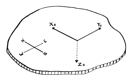
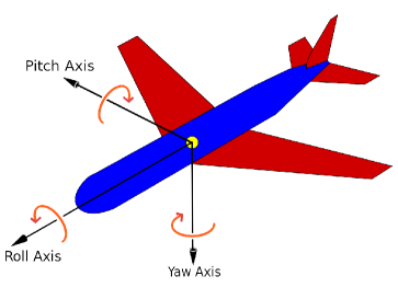
a) b)

Figure 1: a) Earth frame and b) body frame.

The body frame or aircraft referential is defined as in figure 1 (b), where $x_{b}$ corresponds to the roll axis, $y_{b}$ to the pitch axes and $z_{b}$ to the yaw axes, oriented downward. The angular velocity vector $(p,q,r)$ is given in this referential, or to be more precise, at each time, in the Galilean referential that is tangent to this referential.

The wind frame, with origin the center of gravity of the aircraft has an axis $x_{w}$, in the direction of the velocity of the aircraft, the axis $z_{w}$ being in the plane of symmetry of the aircraft. The Euler angles that define the orientation of the wind frame in the earth frame are denoted $\chi(t),\gamma(t),\mu(t)$, and are respectively the aerodynamic azimuth or heading angle, the flight path angle and the aerodynamic bank angle, positive if the port side of the aircraft is higher than the starboard side. See figure 2 (a). We go from earth referential to wind referential using first a rotation with respect to $z$ axis by the heading angle $\chi$, then a rotation with respect to $y$ axis by the flight path angle $\gamma$, and last a rotation with respect to $x$ axis by the bank angle $\mu$.

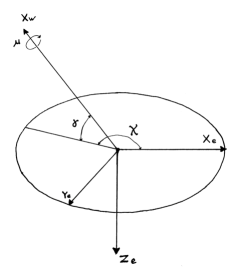
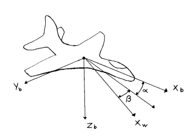
a) b)

Figure 2: a) Wind frame and b) From wind to body frame.

The orientation of the wind frame with respect to the body frame is defined by two angles: the angle of attack $\alpha(t)$ and the sideslip angle $\beta(t)$, which is positive when the wind is on the starboard side of the aircraft, as in figure 2 (b). We go from the wind referential to the body referential using first a rotation with respect to $z$ axis by the side slip angle $\beta$ and then a rotation with respect to $y$ axis by the angle of attack $\alpha$.

5.1.3 Dynamics

In the sequel, we shall write $p(t),q(t),r(t)$ the coordinates of the rotation vector of the body frame with respect to the the earth frame expressed in a frame attached to a Galilean referential, that coincides at time $t$ with the body frame, and $L(t)$, $M(t)$, $N(t)$ the corresponding torques. In the same way $X(t)$, $Y(t)$ and $Z(t)$ denote the forces applied on the aircraft, expressed in a frame attached to a Galilean referential, that coincide at time $t$ with the the wind referential.

5.1.4 Aircraft geometry

The mass of the aircraft is denoted by $m$, $S$ is the surface of the wings. In the body frame, we assume that the aircraft is symmetrical with respect to the $xz$-plane, so that the tensor of inertia has the following form:

$$J:=\left[\begin{matrix}I_{xx}&0&-I_{xz}\\ 0&I_{yy}&0\\ -I_{xz}&0&I_{zz}\end{matrix}\right].$$ (26)

In the standard equations (30), we also need $a$, that stands for the wing span and $b$ for the mean aerodynamic chord.

5.1.5 Forces and torques

The force $(X,Y,Z)$ in the wind frame and the torque $(L,M,N)$ are expressed by the following formulas:

$$X =F(t)\cos(\alpha+\epsilon)\cos(\beta(t))-\frac{\rho}{2}SV(t)^{2}C_{x}-gm\sin{\left(\gamma(t)\right)};$$ (27a)

$$Y =F(t)\cos(\alpha+\epsilon)\sin(\beta(t))+\frac{\rho}{2}SV(t)^{2}C_{y}+gm\cos(\gamma(t))\sin(\mu(t));$$ (27b)

$$Z =-F(t)\sin(\alpha+\epsilon)-\frac{\rho}{2}SV(t)^{2}C_{z}+gm\cos(\gamma(t))\cos(\mu(t));$$ (27c)

$$L =-y_{p}\sin(\epsilon)(F_{1}(t)-F_{2}(t))+\frac{\rho}{2}SV(t)^{2}bC_{l};$$ (27d)

$$M =\frac{\rho}{2}SV(t)^{2}cC_{m};$$ (27e)

$$N =y_{p}\cos(\epsilon)(F_{1}(t)-F_{2}(t))+\frac{\rho}{2}SV(t)^{2}cC_{n}.$$ (27f)

The angle $\epsilon$ is related to the lack of parallelism of the reactors with respect to the $xy-$plane in the body frame and is small.

The aerodynamic coefficients $C_{x},C_{y},C_{z},C_{l},C_{m},C_{n}$ depend on $\alpha$ and $\beta$ and also on the angular speeds $p$, $q$, $r$ and the controls are virtual angles $\delta_{l}$, $\delta_{m}$ and $\delta_{n}$, that respectively express the positions of the ailerons, elevator and rudder.

Remark 84.

One may use $\eta=(F_{1}-F_{2})/(F_{1}+F_{2})$ as an alternative control instead of $\delta_{n}$ in case of rudder jam, where $F_{1}$ and $F_{2}$ represent the thrust of the right and left engines, the sum of which is equal to the total thrust $F$.

5.1.6 Equations

Following Martin [47, 48], the dynamics of the system is modeled by the following set of explicit differential equations (28a–28n,29):

$$\frac{d}{dt}x(t) =V(t)\cos(\chi(t))\cos(\gamma(t));$$ (28a)

$$\frac{d}{dt}y(t) =V(t)\sin(\chi(t))\cos(\gamma(t));$$ (28b)

$$\frac{d}{dt}z(t) =-V(t)\sin(\gamma(t));$$ (28c)

$$\frac{d}{dt}V(t) =\frac{X}{m};$$ (28d)

$$\frac{d}{dt}\gamma(t) =-\frac{Y\sin(\mu(t))+Z\cos(\mu(t))}{mV(t)};$$ (28e)

$$\frac{d}{dt}\chi(t) =\frac{Y\cos(\mu(t))-Z\sin(\mu(t))}{\cos(\gamma(t))mV(t)};$$ (28f)

$$\frac{d}{dt}\alpha(t) =\begin{array}[t]{l}\frac{1}{\cos(\beta(t))}(-p\cos(\alpha(t))\sin(\beta(t))+q\cos(\beta(t))\\ -r\sin(\alpha(t))\sin(\beta(t))+\frac{Z}{mV(t)});\end{array}$$ (28i)

$$\frac{d}{dt}\beta(t) =+p\sin(\alpha(t))-r\cos(\alpha(t))+\frac{Y}{mV(t)};$$ (28j)

$$\frac{d}{dt}\mu(t) =\begin{array}[t]{l}\frac{1}{\cos(\beta(t))}(p\cos(\alpha(t))+r\sin(\alpha(t))\\ +\frac{1}{mV(t)}(Y\cos(\mu(t))\tan(\gamma(t))\cos(\beta(t))\\ -Z(\sin(\mu(t))\tan(\gamma(t))\cos(\beta(t))+sin(\beta(t)))));\end{array}$$ (28n)

$$\left(\begin{array}[]{l}\frac{d}{dt}p(t)\\ \frac{d}{dt}q(t)\\ \frac{d}{dt}r(t)\end{array}\right)=J^{-1}\left(\begin{array}[]{l}(I_{yy}-I_{zz})qr+I_{xz}pq+L\\ (I_{zz}-I_{xx})pr+I_{xz}(r^{2}-p^{2})+M\\ (I_{xx}-I_{yy})pq-I_{xz}rq+N\end{array}\right).$$ (29)

In the last expressions, the terms depending on gravity have been incorporated to the expressions $X$, $Y$ and $Z$, as in [48].

We notice with Martin that this set of equations imply $\cos(\beta)\cos(\gamma)V\neq 0$. The non vanishing of $V$ and $\cos(\beta)$ seems granted in most situations; the vanishing of $V$ may occur with aircrafts equipped with vectorial thrust, which means a larger set of controls, that we won’t consider here. The vanishing of $\cos(\gamma)$ can occur with loopings etc. and would require the choice of a second chart with other sets of Euler angles. According to (28c), the value of $z$ is negative, as in fig. 1 a), the axis $z$ points to the ground.

5.2 The GNA model

In the last equations, $\rho$ can depend on $z$, as the air density vary with altitude. The expression of $C_{x}$ and $C_{z}$ could also depend on $z$ to take in account ground effect. These expressions that depend on $\alpha$, $\beta$, $p$, $q$, $r$, $\delta_{l}$, $\delta_{m}$ and $\delta_{n}$, should also depend on the Mach number, but most available formulas are given for a limited speed range and the dependency on $V$ is limited to the $V^{2}$ term in factor. In the literature, the available expressions are often partial or limited to linear approximations. McLean [49] provides such data for various types of aircrafts; for different speed and flight conditions, including landing conditions with gears and flaps extended.

We have chosen here to use the Generic Nonlinear Aerodynamic (GNA) subsonic models, given by Grauer and Morelli [23] that cover a wider range of values, given in the following table.

$-4\hbox{${}^{\circ}$}\leq\alpha\leq 30\hbox{${}^{\circ}$}$	$-20\hbox{${}^{\circ}$}\leq\beta\leq 20\hbox{${}^{\circ}$}$,
$-100\hbox{${}^{\circ}$}/\mbox{s}\leq p\leq 100\hbox{${}^{\circ}$}/\mbox{s}$	$-50\hbox{${}^{\circ}$}/\mbox{s}\leq q\leq 50\hbox{${}^{\circ}$}/\mbox{s}$	$-50\hbox{${}^{\circ}$}/\mbox{s}\leq r\leq 50\hbox{${}^{\circ}$}/\mbox{s}$
$-10\hbox{${}^{\circ}$}\leq\delta_{l}\leq 10\hbox{${}^{\circ}$}$	$-20\hbox{${}^{\circ}$}\leq\delta_{m}\leq 10\hbox{${}^{\circ}$}$	$-30\hbox{${}^{\circ}$}\leq\delta_{n}\leq 30\hbox{${}^{\circ}$}$

Figure 3: Range of values for the GNA model

Among the 8 aircrafts in their database, we have made simulations with 4: fighters F-4 and F-16C, STOL utility aircraft DHC-6 Twin Otter and the sub-scale model of a transport aircraft GTM (see [28]).

The GNA model depends on 45 coefficients:

$$\begin{array}[]{lll}C_{D}&=&\theta_{1}+\theta_{2}\alpha+\theta_{3}\alpha\tilde{q}+\theta_{4}\alpha\delta_{m}+\theta_{5}\alpha^{2}+\theta_{6}\alpha^{2}\tilde{q}+\theta_{7}\delta_{m}+\theta_{8}\alpha^{3}+\theta_{9}\alpha^{3}\tilde{q}+\theta_{10}\alpha^{4},\\ C_{y}&=&\theta_{11}\beta+\theta_{12}\tilde{p}+\theta_{13}\tilde{r}+\theta_{14}\delta_{l}+\theta_{15}\delta_{n},\\ C_{L}&=&\theta_{16}+\theta_{17}\alpha+\theta_{18}\tilde{q}+\theta_{19}\delta_{n}+\theta_{20}\alpha\tilde{q}+\theta_{21}\alpha^{2}+\theta_{22}\alpha^{3}+\theta_{23}\alpha^{4},\\ C_{l}&=&\theta_{24}\beta+\theta_{25}\tilde{p}+\theta_{26}\tilde{r}+\theta_{27}\delta_{l}+\theta_{28}\delta_{n}\\ C_{m}&=&\theta_{29}+\theta_{30}\alpha+\theta_{31}\tilde{q}+\theta_{32}\delta_{e}+\theta_{33}\alpha\tilde{q}+\theta_{34}\alpha^{2}\tilde{q}+\theta_{35}\alpha^{2}\delta_{e}+\theta_{36}\alpha^{3}\tilde{q}+\theta_{37}\alpha^{3}\delta_{e}+\theta_{38}\alpha^{4},\\ C_{n}&=&\theta_{39}\beta+\theta_{40}\tilde{p}+\theta_{41}\tilde{r}+\theta_{42}\delta_{l}+\theta_{43}\delta_{n}+\theta_{44}\beta^{2}+\theta_{45}\beta^{3},\end{array}$$ (30)

where $\tilde{p}=ap$, $\tilde{r}=ar$, $\tilde{q}=bq$ (see 5.1.4 for the meaning of $a$ and $b$). The aerodynamic coefficient $C_{D}$, $C_{Y}$ and $C_{L}$ are defined by [23, (1)]. The coefficients $C_{x}$ $C_{y}$ and $C_{z}$ in the wind frame are then given by the formulas:

$$\begin{array}[]{lll}C_{x}&=&\cos(\beta)C_{D}-\sin(\beta)C_{Y},\\ C_{y}&=&\sin(\beta)C_{D}+\cos(\beta)C_{Y},\\ C_{z}&=&C_{L}\end{array}$$ (31)

Definition 85.

The simplified model is obtained by replacing $p,q,r$, $\delta_{\ell}$, $\delta_{m}$ an $\delta_{n}$ by $0$ (or some known constants) in the expressions of $C_{x}$, $C_{y}$ and $C_{z}$.

5.3 Block triangular structure of the simplified model

Using the simplified model, the order matrix, where $-\infty$ terms do not appear for better readability, is the following:

$$\begin{array}[]{l}\phantom{\eqref{eq::aircraft1:x}}\begin{array}[]{cccc||ccc||cccc||ccc||ccc}\phantom{x\hskip-0.48ptx}&\hbox to5.0pt{\hss{$x$}\hss}&\hbox to5.0pt{\hss{$y$}\hss}&\hbox to5.0pt{\hss{$z$}\hss}&\hbox to5.0pt{\hss{$V$}\hss}&\hbox to5.0pt{\hss{$\gamma$}\hss}&\hbox to5.0pt{\hss{$\chi$}\hss}&\hbox to5.0pt{\hss{$\alpha$}\hss}&\hbox to5.0pt{\hss{$\beta$}\hss}&\hbox to5.0pt{\hss{$\mu$}\hss}&\hbox to5.0pt{\hss{$F$}\hss}&\hbox to5.0pt{\hss{$p$}\hss}&\hbox to5.0pt{\hss{$q$}\hss}&\hbox to5.0pt{\hss{$r$}\hss}&\hbox to5.0pt{\hss{$\delta_{\ell}$}\hss}&\hbox to5.0pt{\hss{$\delta_{m}$}\hss}&\hbox to5.0pt{\hss{$\delta_{n}$}\hss}\end{array}\\ \begin{array}[]{c}\eqref{eq::aircraft1:x}\\ \eqref{eq::aircraft1:y}\\ \eqref{eq::aircraft1:z}\\ \hline\cr\hline\cr\eqref{eq::aircraft1:V}\\ \eqref{eq::aircraft1:gamma}\\ \eqref{eq::aircraft1:chi}\\ \hline\cr\hline\cr\eqref{eq::aircraft1:alpha}\\ \eqref{eq::aircraft1:beta}\\ \eqref{eq::aircraft1:mu}\\ \hline\cr\hline\cr(\ref{eq::aircraft2}\hbox{p})\\ (\ref{eq::aircraft2}\hbox{q})\\ (\ref{eq::aircraft2}\hbox{r})\end{array}\left(\begin{array}[]{ccc||ccc||cccc||ccc||ccc}1&&&0&0&0&&&&&&&&&&\\ &1&&0&0&0&&&&&&&&&&\\ &&1&0&0&&&&&&&&&&&\\ \hline\cr\hline\cr&&0&1&&&0&0&&0&&&&&&\\ &&0&0&1&&0&0&0&0&&&&&&\\ &&0&0&0&1&0&0&0&0&&&&&&\\ \hline\cr\hline\cr&&0&0&&&1&0&&0&0&0&&&&\\ &&0&0&&&0&1&&0&0&&0&&&\\ &&0&0&0&&0&0&1&0&0&&0&&&\\ \hline\cr\hline\cr&&0&0&&0&&&&0&1&0&0&0&0&0\\ &&0&0&&0&&&&0&0&1&0&0&0&0\\ &&0&0&&0&&&&0&0&0&1&0&0&0\end{array}\right).\end{array}$$

So, algorithm Ō-test provides the following partition, proceeding as in sec. 4.2: with $\Xi_{0}:=\{x,y,z\}$, $\Xi_{1}:=\{V,\gamma,\chi\}$, $\Xi_{2}:=\{\alpha,\beta,\mu,F\}$, $\Xi_{3}:=\{p,q,r\}$ and $\Xi_{4}:=\{\delta_{\ell},\delta_{m},\delta_{n}\}$ or $\Xi_{4}:=\{\delta_{\ell},\delta_{m},\eta\}$ when differential thrust is used (see rem. 84), we see that, for $1\leq k\leq 3$, $\dot{\Xi}_{i}$ only depends on $\bigcup_{\kappa=0}^{k+1}\Xi_{\kappa}$, so that the model is block triangular with $\Sigma_{1}$ corresponding to (28a–28c), $\Sigma_{2}$ corresponding to (28d–28f), $\Sigma_{3}$ corresponding to (28i–28n) and $\Sigma_{4}$ to (29).

Simple computations show that

$$\left|\frac{\partial P}{\partial\xi}|P\in\Sigma_{1};\>\xi\in\Xi_{1}\right|=-V^{2}\cos(\gamma);\quad\left|\frac{\partial P}{\partial\xi}|P\in\Sigma_{3};\>\xi\in\Xi_{3}\right|=\frac{1}{\cos}(\beta),$$ (32)

that do not vanish. In the same way,

$$\left|\frac{\partial P}{\partial\xi}|P\in\Sigma_{4};\>\xi\in\Xi_{3}\right|=\frac{\rho^{3}}{8}S^{3}V^{6}a^{2}b|J|^{-1}\left|\frac{\partial C_{i}}{\partial\delta_{j}}|(i,j)\in\{\ell,m,n\}^{2}\right|,$$ (33)

does not vanish as the diagonal terms ${\partial C_{i}}/{\partial\delta_{i}}$, $i=\ell,m,n$, are much bigger than the others.

So, to apply th. 57, we only need to consider the rank of the Jacobian matrix

$$\left(\frac{\partial P}{\partial\xi}|P\in\Sigma_{2};\>\xi\in\Xi_{2}\right),$$

which is equal to the rank of the Jacobian matrix

$$\Delta:=\left(\frac{\partial Q}{\partial\xi}|Q\in\{X,\sin(\mu)Y+\cos(\mu)Z,-\cos(\mu)Y+\sin(\mu)Z\};\>\xi\in\Xi_{2}\right).$$ (34)

Proposition 86.

The simplified aircraft is flat when the matrix $\Delta$ has full rank.

Let $\Delta_{\xi}$ be the matrix $\Delta$ where the column corresponding to $\xi\in\Xi_{2}$ has been suppressed. If $|\Delta_{\xi}|\neq 0$ at some point, then $x,y,z,\xi$ is a regular flat output at that point.

Proof.

This is a direct consequence of th. 57 ii). ∎

Example 87.

We can associate a diffiety to our aircraft model, which is defined by $\mathbb{R}^{12}\times\left(\mathbb{R}^{\mathbb{N}}\right)^{4}$, and a derivation ð defined by $\text{\dh}:=\text{\dh}_{0}+\text{\dh}_{1}$, where $\text{\dh}_{1}$ is the trivial derivation on $\left(\mathbb{R}^{\mathbb{N}}\right)^{4}$: $\text{\dh}_{1}:=\sum_{z\in\{F,\delta_{l},\delta_{m},\delta_{n}\}}^{m}\sum_{k\in\mathbb{N}}z_{i}^{(k+1)}\partial/\partial z_{i}^{(k+1)}$ and $\text{\dh}_{0}$ is defined on $\mathbb{R}^{12}$ by the differential equations (28a–28n,29):

$$\delta_{0}:=V(t)\cos{\left(\chi(t)\right)}\cos{\left(\gamma(t)\right)}\frac{\partial}{\partial x}+V(t)\sin{\left(\chi(t)\right)}\cos{\left(\gamma(t)\right)}\frac{\partial}{\partial y}+\cdots$$

In practice, the diffiety is defined a smaller open set, because of the bounds that exist on the variables. The values of the controls are bounded and one wishes to restrict the values of the angle of attack $\alpha$ or side-slip angle $\beta$ for safety reasons. The maximal values for the GNA model are given below in table 3. Other limitations must be included, such as the maximal value of the thrust. The speed $V$ should also be greater than the stalling speed (see 5.5).

We will now consider more closely the possible choices of flat outputs.

5.4 Choices of flat outputs

5.4.1 The side-slip angle choice

Martin [47, 48] has used the set of flat outputs: $x,y,z,\beta$. We need to explicit under which condition such a flat output may be chosen, i.e. when the Jacobian determinant

$$\Delta_{\beta}=\left|\begin{array}[]{ccc}\frac{\partial X}{\partial\alpha}&\frac{\partial X}{\partial\mu}&\frac{\partial X}{\partial F}\\ \frac{\partial(\sin\mu\,Y+\cos\mu\,Z)}{\partial\alpha}&\frac{\partial(\sin\mu\,Y+\cos\mu\,Z)}{\partial\mu}&\frac{\partial(\sin\mu\,Y+\cos\mu\,Z)}{\partial F}\\ \frac{\partial(\cos\mu\,Y-\sin\mu\,Z)}{\partial\alpha}&\frac{\partial(\cos\mu\,Y-\sin\mu\,Z)}{\partial\mu}&\frac{\partial(\cos\mu\,Y-\sin\mu\,Z)}{\partial F}\end{array}\right|$$

does not vanish, according to prop. 86. First, we remark, following Martin [47, p. 80] that when $Y=gm\cos(\gamma)\sin(\mu)$ and $Z=gm\sin(\gamma)\sin(\mu)$, i.e. when the lift is zero, $\sin\mu\,Y+\cos\mu\,Z=gm\cos(\gamma)$ and $\cos\mu\,Y-\sin\mu\,Z=0$, so that the last row of $D_{1}$ is zero and the determinant vanishes. This means that $0$-g flight trajectories are singular for this flat output. On the other hand, when $\beta$ and $\alpha$ are close to $0$, which is the case in straight and level flight, easy computations using eq. (27a–27c) allow Martin to conclude that

$$|\Delta_{\beta}|\approx-Z\left(\frac{\rho}{2}SV^{2}\frac{\partial C_{z}}{\partial\alpha}+F\right)\gg 0.$$

To go further, one may use the expression of $X$ eq (27a) and deduce from it

$$F=\frac{X+\frac{\rho}{2}SV^{2}C_{x}+gm\sin(\gamma)}{\cos(\alpha+\epsilon)\cos(\beta)},$$ (35)

assuming $\cos(\alpha+\epsilon)\cos(\beta)$. Substituting this expression in $Y$ and $Z$, we define $\tilde{Y}$ and $\tilde{Z}$ and further define $\hat{Y}:=\cos(\mu)\tilde{Y}-\sin(\mu)\tilde{Z}$ and $\hat{Z}:=\sin(\mu)\tilde{Y}+\cos(\mu)\tilde{Z}$. Then, $|\Delta_{\beta}|\neq 0$ when

$$\left|\begin{array}[]{cc}\frac{\partial\hat{Y}}{\partial\alpha}&\frac{\partial\hat{Y}}{\partial\mu}\\ \frac{\partial\hat{Z}}{\partial\alpha}&\frac{\partial\hat{Z}}{\partial\mu}\end{array}\right|\neq 0.$$ (36)

The main interest of this choice is to be able to impose easily $\beta=0$, which is almost always required.

5.4.2 The bank angle choice

As the angle $\mu$ is known, we may compute from $\Xi_{1}^{\prime}$ and $\Xi_{1}^{\prime\prime}$ the values $X$, $Y$ and $Z$. So, singularities for this flat outputs are such that

$$|\Delta_{\mu}|=\left|\begin{array}[]{ccc}\frac{\partial X}{\partial\alpha}&\frac{\partial X}{\partial\beta}&\frac{\partial X}{\partial F}\\ \frac{\partial Y}{\partial\alpha}&\frac{\partial Y}{\partial\beta}&\frac{\partial Y}{\partial F}\\ \frac{\partial Z}{\partial\alpha}&\frac{\partial Z}{\partial\beta}&\frac{\partial Z}{\partial F}\end{array}\right|\neq 0$$ (37)

Using $\tilde{Y}$ and $\tilde{Z}$, as defined in subsec. 5.4.1, we see that this is equivalent to

$$\left|\begin{array}[]{cc}\frac{\partial\hat{Y}}{\partial\alpha}&\frac{\partial\hat{Y}}{\partial\beta}\\ \frac{\partial\hat{Z}}{\partial\alpha}&\frac{\partial\hat{Z}}{\partial\beta}\end{array}\right|\neq 0.$$ (38)

When $\beta$ is $0$, $\partial\tilde{Z}/\partial\beta$ is also $0$, due to the aircraft symmetry. Using the GNA model (see 5.2), we have $\partial C_{x}/\beta=0$ and $\partial C_{z}/\partial\beta=0$, so that $\partial\tilde{Z}/\partial\beta=0$. The value of the determinant (38) is then

$$-\frac{\partial\hat{Z}}{\partial\alpha}\frac{\partial\hat{Y}}{\partial\beta}.$$ (39)

For most aircrafts, $\partial C_{y}/\partial\beta$ is negative at $\beta=0$, with values in the range $[-1.,-0.5]$. Delta wing aircrafts seem to be a exception, with smaller absolute values ($-0.014$ for the X-31) or even negative ones ($+0.099$ for the F-16XL). It seems granted that for regular transport planes, $\partial C_{y}/\partial\beta$ is negative, so that the determinant vanishes only when $\partial\tilde{Z}/\partial\alpha$ is $0$. We will see in 5.5 that this may be interpreted as stalling condition and that the vanishing of (39) on a trajectory with constant controls means that the points of this trajectory are flat singularities, so that no other flat outputs could work.

This choice is the best to impose $\mu=0$ and is natural for decrabe maneuver, that is when landing with a lateral wind, which implies $\beta\neq 0$. We then need to maintain $\mu$ close to $0$ to avoid the wings hitting the runway.

It is also a good choice when $Y=Z=0$, a situation that may be encountered in aerobatics or when training for space condition with $0$-g flights (see subsec 7.2). The choices $\beta$ and $\mu$ are compared in [57, 7.1] with the simulation of a twin otter flying with one engine.

5.4.3 The thrust choice

The choice of thrust $F$ has one main interest: to set $F=0$ and consider the case of a aircraft having lost all its engines. The aircraft must land by gliding when all engines are lost. This is a rare situation, but many successful examples are known, including the famous US Airways Flight 1549 [5]. The singularities of this flat output are such that

$$|\Delta_{F}|=\left|\begin{array}[]{ccc}\frac{\partial X}{\partial\alpha}&\frac{\partial X}{\partial\mu}&\frac{\partial X}{\partial\beta}\\ \frac{\partial(\sin\mu\,Y+\cos\mu\,Z)}{\partial\alpha}&\frac{\partial(\sin\mu\,Y+\cos\mu\,Z)}{\partial\mu}&\frac{\partial(\sin\mu\,Y+\cos\mu\,Z)}{\partial\beta}\\ \frac{\partial(\cos\mu\,Y-\sin\mu\,Z)}{\partial\alpha}&\frac{\partial(\cos\mu\,Y-\sin\mu\,Z)}{\partial\mu}&\frac{\partial(\cos\mu\,Y-\sin\mu\,Z)}{\partial\beta}\end{array}\right|$$

vanishes. When $F=0$, by eq. (27a–27c), the vanishing of $D_{3}$ is equivalent to

$$\left|\begin{array}[]{ccc}\frac{\partial C_{x}}{\partial\alpha}&0&\frac{\partial C_{x}}{\partial\beta}\\ \frac{\partial(\cos\mu\,C_{z})}{\partial\alpha}&\frac{\partial(\sin\mu\,C_{y}+\cos\mu\,C_{z})}{\partial\mu}&\frac{\partial(\sin\mu\,C_{y})}{\partial\beta}\\ \frac{\partial(-\sin\mu\,C_{z})}{\partial\alpha}&\frac{\partial(\cos\mu\,C_{y}-\sin\mu\,C_{z})}{\partial\mu}&\frac{\partial(\cos\mu\,C_{y})}{\partial\beta}\end{array}\right|=\frac{\partial C_{x}}{\partial\alpha}\left(C_{y}\frac{\partial C_{y}}{\partial\beta}-C_{z}\frac{\partial C_{x}}{\partial\beta}\right).$$

When $\beta$ vanishes, $C_{y}$ and $\partial C_{z}/\partial\beta$ also vanish, due to the aircraft symmetry with respect to the $xz$-plane. So, we need have $\beta\neq 0$ to use those flat outputs. Using the GNA model, $C_{x}$ and $C_{z}$ depend only on $\alpha$ and $C_{y}$ depends linearly on $\beta$.

In the case of a gliding aircraft, situations with $\beta\neq 0$ could precisely be useful to achieve the forward slip maneuver. When the aircraft is too high, combining non zero $\beta$ and $\mu$ precisely allows a fast descent while keeping a moderate speed. This is very useful when gliding, as there is no option for a go around when approaching the landing strip too high or too fast. This maneuver was performed with success by the “Gimli Glider” [46], Air Canada Flight 143, that ran out of fuel on July 23, 1983, which could land safely in Gimli former Air Force base. A simulation of the forward slip may be found in [57, 7.2].

5.4.4 Other sets of flat outputs

Among the other possible choices for completing the set $\Xi_{1}$ in order to get flat outputs, the interest of $\alpha$ is mostly academic. Indeed,

$$\Delta_{\alpha}=\left|\begin{array}[]{ccc}\frac{\partial X}{\partial\beta}&\frac{\partial X}{\partial\mu}&\frac{\partial X}{\partial F}\\ \frac{\partial(\sin\mu\,Y+\cos\mu\,Z)}{\partial\beta}&\frac{\partial(\sin\mu\,Y+\cos\mu\,Z)}{\partial\mu}&\frac{\partial(\sin\mu\,Y+\cos\mu\,Z)}{\partial F}\\ \frac{\partial(\cos\mu\,Y-\sin\mu\,Z)}{\partial\beta}&\frac{\partial(\cos\mu\,Y-\sin\mu\,Z)}{\partial\mu}&\frac{\partial(\cos\mu\,Y-\sin\mu\,Z)}{\partial F}\end{array}\right|$$

Then, $|\Delta_{\alpha}|=0$ when

$$\left|\begin{array}[]{cc}\frac{\partial\hat{Y}}{\partial\beta}&\frac{\partial\hat{Y}}{\partial\mu}\\ \frac{\partial\hat{Z}}{\partial\beta}&\frac{\partial\hat{Z}}{\partial\mu}\end{array}\right|=0.$$ (40)

Easy computations show that it is the case when $\mu=\beta=0$, so that $\alpha$ is not a suitable alternative input near stalling conditions, except possibly when $\mu\neq 0$. But mostly, our aerodynamic model cannot fully reflect the real behavior near stalling so that it seems safe to exclude stalling a.o.a from the domain of definition.

One may also consider time-varying expressions, e.g. linear combinations of $\beta$ and $\mu$, to smoothly go from one choice to another.

5.5 Stalling conditions

It is known that the lift of a wing reaches a maximum at a critical angle of attack, due to flow separation. This phenomenon can be hardly reversible and creates a sudden drop of the lift force $Z$ from its peack value. Our mathematical model is too poor to fully reflect such behavior, but a maximum for the lift can still be computed.

We need to take also in account the contribution of the thrust in the expression of $Z$, and simple computations show that the critical angle of attack corresponds in our setting to a maximum of $\tilde{Z}$, that is $\partial\tilde{Z}/\partial\alpha=0$, which corresponds to the singularity for flat output $\mu$ already observed above (39).

Three cases may appear with stalling:

1) to reach an extremal value of $\tilde{Z}$, meaning that $\partial\tilde{Z}/\partial\alpha$ vanishes;

2) to reach the maximum thrust $F_{\mbox{max}}$ before reaching a maximum of $\tilde{Z}$;

3) reaching no maximum of $\tilde{Z}$ with a aircraft with trust/weight ratio greater than $1$: in such a case, there is no stalling.

For horizontal straight line trajectories, we may compute the speed $V$ and the thrust $F$, depending on $\alpha$, for $\beta=\mu=0$, using the simplified model. We may also use the full model. As $\alpha$, $\beta$ and $\mu$ are constants, $p=q=r=0$, which further allows to express $\delta_{\ell}$, $\delta_{m}$ and $\delta_{n}$ depending on $\alpha$, so that $C_{\ell}=C_{m}=C_{n}=0$, which is easy with the GNA model that is linear in those quantities.

E.g., For the F4, setting the weight to $38924\mbox{lb}$ [23], the evaluated stall speed, angle of attack and thrusts are respectively $67.6789$m/s ($131.56$kn), $0.4200\mbox{rad}$ ($24.07\hbox{${}^{\circ}$}$) and $77.0436$ for the full model and $64.0904$m/s, $0.4366\mbox{rad}$ and $78.8806$ for the simplified one, without thrust limitations. These thrust values are below the thrust of J79-GE-17A engines of later versions ($79.38$kN with afterburning). Assuming a maximal thrust of $2\times 71.8\mbox{kN}$, that corresponds to the J79-GE-2 engines of the first production aircrafts, the stall speed and angle of attack are $67.9835$m/s and $0.3969\mbox{rad}$ with the full model, $64.5515$m/s and $0.4057\mbox{rad}$ with the simplified one. The full model stall speed of about $132$kn agrees more or so with the stall speed values of $146\mbox{KCAS}$ or $148\mbox{KCAS}$, according to the models, computed with the NATOPS manual [51, fig. 4.1 and 4.2] at $10000$ ft and below and the computed a.o.a of $23\hbox{${}^{\circ}$}$ with the indicated stall a.o.a of $27$ to $28$ “units”, keeping in mind that those units are not exactly degrees and that our mathematical definition of stalling cannot fully match the actual behavior. See fig. 4.

We notice in the figure that the curves become unrealistic outside the range of values of the GNA model given in fig. 3, so that $F$ even takes negative values for $\alpha<0.065\mbox{rad}$, which is very close to the $-4\hbox{${}^{\circ}$}$ limit.

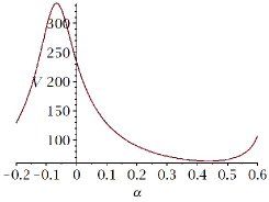
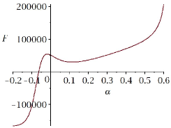
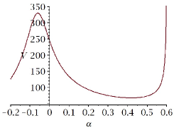
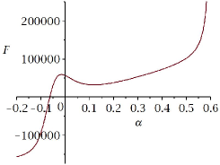
a) b) c) d)

Figure 4: F-4: values of $V$ and $F$ depending on $\alpha$. a) & b) full generic nonlinear aerodynamic model; c) & d) simplified model

We have the following theorem, that shows that stalling condition means that the system is not flat for some trajectories with $\beta=\mu=0$.

Theorem 88.

Let a trajectory be such that $\alpha$, $\beta$, $\mu$, $F$, $\gamma$ and $V$ are constants, with moreover $\beta=0$, $\alpha$ and $V$ respectively equal to the stall a.o.a. and stall speed. There is no flat point in this trajectory.

Proof.

Simple computations show that when $\beta=0$, $\alpha$ is equal to stalling a.o.a and $V$ the stall speed, the rank of the Jacobian matrix $(\partial P/\partial x\mid P\in\Sigma_{2},\>x\in\Xi_{3})$ is at most $3$. This is then a straightforward consequence of th. 83, noticing that $\chi^{\prime}$ is the only term involving $\chi$ in the equations and that it appears linearly. ∎

5.6 Restricted model with 9 state functions

When foccussing on flight handling quality, one may restrict to $9$ state variables by neglecting $x$, $y$ and $\chi$ and suppressing equations (28a,28b28f), as those variables do not appear in the remaining $9$ equations. We get then the order matrix:

$$\begin{array}[]{l}\phantom{\eqref{eq::aircraft1:x}}\begin{array}[]{cc||cc||cccc||ccc||ccc}\phantom{x\hskip-0.48ptx}&\hbox to5.0pt{\hss{$z$}\hss}&\hbox to5.0pt{\hss{$V$}\hss}&\hbox to5.0pt{\hss{$\gamma$}\hss}&\hbox to5.0pt{\hss{$\alpha$}\hss}&\hbox to5.0pt{\hss{$\beta$}\hss}&\hbox to5.0pt{\hss{$\mu$}\hss}&\hbox to5.0pt{\hss{$F$}\hss}&\hbox to5.0pt{\hss{$p$}\hss}&\hbox to5.0pt{\hss{$q$}\hss}&\hbox to5.0pt{\hss{$r$}\hss}&\hbox to5.0pt{\hss{$\delta_{\ell}$}\hss}&\hbox to5.0pt{\hss{$\delta_{m}$}\hss}&\hbox to5.0pt{\hss{$\delta_{n}$}\hss}\end{array}\\ \begin{array}[]{c}\eqref{eq::aircraft1:z}\\ \hline\cr\hline\cr\eqref{eq::aircraft1:V}\\ \eqref{eq::aircraft1:gamma}\\ \hline\cr\hline\cr\eqref{eq::aircraft1:alpha}\\ \eqref{eq::aircraft1:beta}\\ \eqref{eq::aircraft1:mu}\\ \hline\cr\hline\cr(\ref{eq::aircraft2}\hbox{p})\\ (\ref{eq::aircraft2}\hbox{q})\\ (\ref{eq::aircraft2}\hbox{r})\end{array}\left(\begin{array}[]{c||cc||cccc||ccc||ccc}1&0&0&&&&&&&&&&\\ \hline\cr\hline\cr 0&1&&0&0&&0&&&&&&\\ 0&0&1&0&0&0&0&&&&&&\\ \hline\cr\hline\cr 0&0&&1&0&&0&0&0&&&&\\ 0&0&&0&1&&0&0&&0&&&\\ 0&0&0&0&0&1&0&0&&0&&&\\ \hline\cr\hline\cr 0&0&&0&&&0&1&0&0&0&0&0\\ 0&0&&0&&&0&0&1&0&0&0&0\\ 0&0&&0&&&0&0&0&1&0&0&0\end{array}\right).\end{array}$$

Following the construction of subsec. 4.2, as we did in subsec. 5.3, we define $\bar{\Xi}_{0}:=\{z\}$, $\bar{\Xi}_{1}:=\{V,\gamma\}$, $\bar{\Xi}_{2}:=\{\alpha,\beta,\mu,F)=\Xi_{2}$, $\bar{\Xi}_{3}:=\{p,q,r\}=\Xi_{3}$ and $\bar{\Xi}_{4}:=\{delta_{\ell},\delta_{m},\delta_{n}\}=\Xi_{4}$, we see that, for $1\leq k\leq 3$, $\dot{\Xi}_{i}$ only depends on $\bigcup_{\kappa=0}^{k+1}\Xi_{\kappa}$, so that this new model is also block triangular with $\bar{\Sigma}_{1}$ corresponding to (28c), $\bar{\Sigma}_{2}$ corresponding to (28d–28e), $\Sigma_{3}$ corresponding to (28i–28n) and $\Sigma_{4}$ to (29). It is easily seen that the only Jacobian matrix that may possibly not be of full rank is $(\partial P/\partial\xi|(P,\xi\in\bar{\Sigma}_{2}\times\Xi_{2})$. As it is a submatrix of $(\partial P/\partial\xi|(P,\xi\in\Sigma_{2}\times\Xi_{2})$, points that do not satisfy the regularity condition of th. 57 for the $9$ state variables system do not satify it for the $12$ state variables system. We can associate to this ō-system $12$ possible sets of linearizing outputs: first, we take $\xi_{1}=z$, then $\xi_{2}\in\bar{\Xi}_{1}$ (2 possibilities) and $\{\xi_{3},\xi_{4}\}\in\bar{\Xi}_{2}$ (6 possibilities).

6 Simulations using the simplified flat model

In this section, we show simulations done with the flat approximation of the model. These simulations are conducted with the classical set of flat outputs described in section 5.4.1, that is $x,y,z,\beta$.

As mentioned above, the flat approximation was obtained by neglecting the dependency of $C_{x},C_{y},C_{z}$ on $p,q,r,\delta_{l},\delta_{m},\delta_{n}$. Comparing with the full aircraft model considered in the next section, no significant change of behaviour could be noticed. We show here that the model remains robust to various perturbations in the expression of the forces.

This tends to show that in many contexts the flat approximation is quite sufficient.

Moreover, we show that the flat model allows a high flexibility in trajectory planning and tracking.

All these suitable properties remain when one reactor is out of order.

6.1 Theoretical setting for feed-back design

The great advantage of flatness is that the flat motion planning makes an open loop control immediately available. When a closed loop is required, the feedback is designed from the difference between the actual values of the flat outputs and their reference values, so that this difference, being the solution of some differential equation, tends to zero. The reader may refer to [6] for more robust approach of the control of flat systems.

In the framework of the flat aircraft model, the feedback is done is two stages. Indeed the dependency of the system variables on $F,p,q,r$ has a slow dynamics in comparison to the rapidity of the dynamics that controls $p,q,r$ from $\delta_{l},\delta_{m},\delta_{n}$. This allows to construct a cascade feedback, as done in [48]. More precisely, one can build a dynamic linearizing feedback that allows controlling the partial state vector $\Xi=(x,y,z,V,\alpha,\beta,\gamma,\chi,\mu,F)$ using the command $\dot{F},p,q,r$, which allows following the reference trajectories of the flat outputs $x,y,z,\beta$, using static linearizing feedback. More precisely, one can compute a vector valued function $\Delta_{0}$ and a matrix valued function $\Delta_{1}$, both depending on $x,y,z,V,\alpha,\beta,\gamma,\chi,\mu,F$ such that:

$$\left(\begin{array}[]{c}x^{(3)}\\ y^{(3)}\\ z^{(3)}\\ \dot{\beta}\end{array}\right)=\Delta_{0}+\Delta_{1}\left(\begin{array}[]{c}p\\ q\\ r\\ \dot{F}\end{array}\right)$$

At this stage, the variables $p,q,r,\dot{F}$ are seen as commands. In order to make the system linear, one introduces a new vector valued command $v$, such that:

$$\left(\begin{array}[]{c}p\\ q\\ r\\ \dot{F}\end{array}\right)=\Delta_{1}^{-1}(v-\Delta_{0})$$

Eventually the command $v$ is chosen of the form:

$$v(t)=\left(\begin{array}[]{c}P_{0}(x_{\hbox{ref}}(t)-x(t))+P_{1}(\dot{x}_{\hbox{ref}}(t)-\dot{x}(t))+P_{2}(\ddot{x}_{\hbox{ref}}(t)-\ddot{x}(t))+P_{3}x_{\hbox{ref}}^{(3)}(t)\\ P_{0}(y_{\hbox{ref}}(t)-y(t))+P_{1}(\dot{y}_{\hbox{ref}}(t)-\dot{y}(t))+P_{2}(\ddot{y}_{\hbox{ref}}(t)-\ddot{y}(t))+P_{3}y_{\hbox{ref}}^{(3)}(t)\\ P_{0}(z_{\hbox{ref}}(t)-z(t))+P_{1}(\dot{z}_{\hbox{ref}}(t)-\dot{z}(t))+P_{2}(\ddot{z}_{\hbox{ref}}(t)-\ddot{z}(t))+P_{3}z_{\hbox{ref}}^{(3)}(t)\\ -k_{1}(\beta_{\hbox{ref}}(t)-\beta(t))+\dot{\beta}_{\hbox{ref}}(t),\end{array}\right)$$

where $P(X)=P_{0}+P_{1}X+P_{2}X^{2}+P_{X}^{3}$ is actually the following polynomial $P(X)=(X-k_{1})^{3}$. Therefore the error function $e_{s}(t)=s_{\hbox{ref}}(t)-s(t)$ satisfies the following differential equations $P(e_{s}(t))=0$. In our experiments, $k_{1}=-5$, so that $e_{s}(t)\underset{t\rightarrow+\infty}{\longrightarrow}0$, for each value of $s$ in $x,y,z,\beta$. The value of $k_{1}$ has tuned manually and is similar to values found in [47].

In a second stage the variables $p,q,r$ are controlled through a static linearizing feedback based on $\delta_{l},\delta_{m},\delta_{n}$. This part of the system, as mentioned above, is fast in comparison to the first part. More precisely, one can compute the vector valued function $\Lambda_{0}$ and a matrix valued function $\Lambda_{1}$, both depending on $V,\alpha,\beta,p,q,r$ such that:

$$\left(\begin{array}[]{c}\dot{p}\\ \dot{q}\\ \dot{r}\\ \end{array}\right)=\Lambda_{0}+\Lambda_{1}\left(\begin{array}[]{c}\delta_{l}\\ \delta_{m}\\ \delta_{n}\\ \end{array}\right)$$

Then as previously, one introduced a new command $w$ such that

$$\left(\begin{array}[]{c}\delta_{l}\\ \delta_{m}\\ \delta_{n}\\ \end{array}\right)=\Lambda_{1}^{-1}(w-\Lambda_{0})$$

and

$$w=\left(\begin{array}[]{c}-k_{2}(p_{\hbox{ref}}(t)-p(t))+\dot{p}_{\hbox{ref}}(t)\\ -k_{2}(q_{\hbox{ref}}(t)-q(t))+\dot{q}_{\hbox{ref}}(t)\\ -k_{2}(r_{\hbox{ref}}(t)-r(t))+\dot{r}_{\hbox{ref}}(t)\\ \end{array}\right),$$

where $k_{2}=-15$ in our experiments. Therefore $s(t)-s_{\hbox{ref}}(t)\underset{t\rightarrow+\infty}{\longrightarrow}0$, for $s\in\{p,q,r\}$.

The rational behind this cascade feedback is the following. The variables $(x,y,z,V,\alpha,\beta,\gamma,\chi,\mu,F)$ are slowly controlled through $\dot{F},p,q,r$. Once the required values of $p,q,r$ are known, they are quickly reached through the control performed with $\delta_{l},\delta_{m},\delta_{n}$. The respective values of $k_{1}$ and $k_{2}$ reflect the disparity of speed between the two dynamics. See e.g. [35, 62] and the references therin for a singular perturbation approach of such systems.

6.2 Conventions used in our simulations

We now show a series of experiments that illustrate the strength of the flat approximation to control the aircraft in various situations. Those experiments were all performed with GTM extracted from [28]. The implementation is made in Python, relying on the symbolic library sympy, the numerical array library numpy and the numerical integration of ODE systems from the library scipy.

The experiments are all about following a reference trajectory defined by the following expressions:

$$\left\{\begin{array}[]{rcl}x_{\hbox{ref}}(t)&=&V_{1}\cos(\pi(t-T_{\hbox{initial}})/(T_{\hbox{final}}-T_{\hbox{initial}}))\\ y_{\hbox{ref}}(t)&=&V_{1}\sin(\pi(t-T_{\hbox{initial}})/(T_{\hbox{final}}-T_{\hbox{initial}}))\\ z_{\hbox{ref}}(t)&=&-V_{2}t-1000\\ \beta_{\hbox{ref}}(t)&=&0\end{array}\right.,$$

where $T_{\hbox{initial}}=0s,T_{\hbox{final}}=30s,V_{1}=30ms^{-1},V_{2}=5ms^{-1}$. This reference trajectory is an upward helix.

6.3 Initial perturbation

We carried out experiments where the aircraft started away from the reference trajectory and then joined it after a few seconds. If the initial perturbation is not too big, the feedback alone is capable to attract the aircraft to the reference trajectory. If the initial starting point is really far away from the reference trajectory, the flexibility of the flatness based approach allows designing very easily transition trajectory which can be followed with the feedback and that brings to aircraft to the reference upward helix trajectory.

The experiment is moreover performed when a one reactor is broken. We observe that the actual trajectory of the aircraft merges with the reference one, as shown in figure 5. The reference and the actual trajectories merge perfectly, even when starting from a point off the trajectory. In [57, fig. 2], the power of one engine is slowly reduced, so that one can see the variation of state functions, such as bank angle.

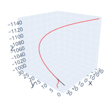
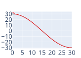
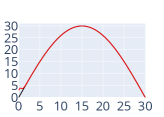
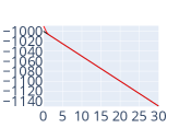
a)  simulated trajectory with initial perturbation reference trajectory $x\>(\mbox{m})$ b) time (s) $y\>(\mbox{m})$ c) time (s) $z\>(\mbox{m})$ d) time (s) $\beta\>(\mbox{rad})$ e) time (s)

Figure 5: The values of the GTM trajectory, one engine: the aircraft converges toward the reference trajectory. a) Trajectory, $3$D view; b)–e) Histories of $x,y,z,\beta$

6.4 Variable wind

In this section, we address the most critical problem about the flat approximation. Since the dependency of the aerodynamic coefficient on $p,q,r,\delta_{l},\delta_{m},\delta_{n}$ is discarded, one can wonder if the model is robust enough to significant perturbations in the values of the thrust. It turns out that under mild external forces, the model remains reliable.

In the last experiment, the motion of the aircraft is perturbed by a variable wind. This perturbation force is a sinusoidal function which amplitude is 50lbf and frequency is 0.1Hz. This perturbation is assumed to roughly model a quasi-periodic change in wind direction. Doing a more realistic analysis is beyond our scope.

This setting is applied to the GTM with the piece-wise trajectory defined above. We observe a very robust behavior of the model, as rendered in figures 6 and 7. The reference and the actual trajectories still merge perfectly with a variable wind. For the variables $F,\alpha,p,q,r$ variations due to the variable wind are noticeable in the graphs.

$x\>(\mbox{m})$ a) time (s) $y\>(\mbox{m})$ b) time (s) $z\>(\mbox{m})$ c) time (s)

Figure 6: Variable wind. a)–d) Histories of $x,y,z$

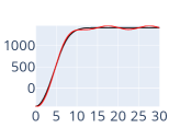
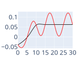
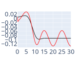
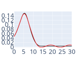
$F\>(\mbox{N})$ a) time (s) $\mu\>(\mbox{rad})$ b) time (s) $p\>(\mbox{rad}/\mbox{s})$ c) time (s) $q\>(\mbox{rad}/\mbox{s})$ d) time (s)

Figure 7: Variable wind. a)–e) Histories of $F,\mu,p,q$

7 Simulations using the full model

7.1 Implementation in Maple

Our implementation computes power series approximations of all state variables and control at regular time interval. We proceed in the same way for the feed-back, which is also approximated with power series at the same time interval for better efficiency during numerical integration.

The structure of the equations implies the existence of a lazy flat parametrization, as shown by th. 49. Moreover, it means that the requested power series can be computed in a fast way using Newton’s method, when initialized with suitable values. Most of the time, values for state variables such as $\beta$ or $\alpha$ are close to $0$. If not, calibration functions can give e.g. the value of $\alpha$, assuming that $V$, $\gamma^{\prime}$, $\chi$, $\beta$ and $\mu$ are constants. See [57, § 4] for more details.

We denote by $\hat{\xi}(t)$ the planed function for any state variable $\xi$, according to the motion planning using the simplified flat system and the choice of $\hat{x}$, $\hat{y}$, $\hat{z}$ and $\hat{\beta}$ (or $\hat{\mu}$). We also denote by $\updelta\xi$ the difference $\xi-\hat{\xi}$ between the planed trajectory and the trajectory computed with the full model. We did not manage to get a working feed-back without using integrals $I_{1}$, $I_{2}$, $I_{3}$, $I_{4}$ of $\cos(\chi)\updelta x+\sin(\chi)\updelta y$, $-\sin(\chi)\updelta x+\cos(\chi)\updelta y$, $\updelta z$ and $\updelta\beta$ (or $\updelta\mu$) respectively. When using the flat outputs $x,y,z,F$, $I_{4}$ is no longer needed.

For the feed-back, we choose positive real numbers $\lambda_{i,j}$, with $1\leq i\leq 4$, and $1\leq j\leq 5$ for $i=2$ or $i=3$ and $1\leq j\leq 3$ for $i=1$ or $i=4$. The value of $\updelta F$, $\updelta\delta_{l}$, $\updelta\delta_{m}$, $\updelta\delta_{n}$, are computed, so that $\prod_{i=1}^{3}(d/dt+\lambda_{1,i})I_{1}=0$, $\prod_{i=1}^{3}(d/dt+\lambda_{4,i})I_{4}=0$, $\prod_{i=1}^{5}(d/dt+\lambda_{2,i})I_{2}=0$, $\prod_{i=1}^{5}(d/dt+\lambda_{3,i})I_{3}=0$, using the derivation $d/dt$ of the linearized simplified system around the planed trajectory. Then, we use the controls $\hat{\delta}_{l}+\updelta\delta_{l}$, $\hat{\delta}_{m}+\updelta\delta_{m}$, $\hat{\delta}_{n}+\updelta\delta_{n}$, $\hat{F}+\updelta F$ in the numerical integration. If the $\updelta\xi$ are small enough to behave like the $\mathrm{d}\xi$ of the linearized system, and the solution of the full model not too far from the planed solution of the simplified model, the convergence is granted.

In practice, the choice of suitable $\lambda_{i,j}$ is difficult and empirical: two small, the trajectory is lost, two high, increasing oscillations may appear. We neglect here the dynamics of the actuator, our goal being to show that the feed-back is able to provide a solution for the full model, using the trajectory planed with the simplified one, the linearizing outputs remaining close to their original values. The feedback used here relies on a linear approximation around the planned trajectory. I has the advantage of fast computation but will not work any more when perturbations are too great. One may refer e.g. to [6] or [74] for more robust control of flat systems.

Unless otherwise stated, angles are expressed in radians, lengths in meters, times in seconds, thrusts in Newtons, masses in kg. Curves in red correspond to the planed trajectory $\hat{\xi}$, while curves in blue correspond to the integration of the full model. For more clarity $z$ has been replaced by $-z$ to get positive values when drawing curves.

Computation times are given using Maple 19 with an Intel processor Core i5 $2.5$GHz. These are just indications that can vary from a session to another.

7.2 Using flat outputs with $\mathbf{\mu}$. Gravity-free flight with the F16

We experiment here a $0$-g flight with a parabolic trajectory, using the F-16 model for which $C_{z}$ vanishes for a value of $\alpha$ close to $-0.016$ rad. See fig. 8, where $\updelta z$ corresponds to the difference between the reference altitude and the altitude of the simulated model. For this simulation, we used an expression of air density $\rho(z)$ varying with altitude $z$, following Martin [47, A.16 p. 97]. The total computation time of the simulation is $371$s.

$$\begin{array}[]{ll}x&=750t\mathrm{km}/\mathrm{h};\quad y=0;\quad z=g\frac{t^{2}}{2}-2000;\quad\mu=0;\\ \lambda_{i,j}&=5.;\\ \rho(z)&=1.225(1+0.0065z/288.15)^{(9.80665/287.053\times 0.0065-1)}\end{array}$$ (41)

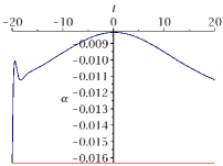
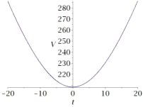
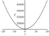
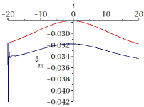
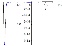
a) b) c) d) e)

Figure 8: F-16 $0$-g flight. a) $\alpha\>(\mbox{rad})$; b) $V\>(\mbox{m}/\mbox{s})$; c) $F\>(\mbox{N})$; d) $\delta_{m}\>(\mbox{rad})$ and e) $\updelta z\>(\mbox{m})$.

8 Conclusion

We have introduced a notion of oudephippical systems, or ō-systems, that generalizes many special cases of chained or triangular systems previously know in the control literature. We further gave algorithms to test in polynomial time if a given system belongs to this category and to test regularity conditions that are sufficient to imply that the system is flat at a some point.

Then, as the flat outputs are state variables, the computation of the flat parametrization and the design of a feedback to stabilize the system around the planned trajectory are computationally easy, even for non trivial systems, such as the aircraft model used as an illustration. This model is flat if one neglects some terms and our simulations show that a suitable feedback is able to compensate model errors due to this simplification.

The systematic study of all possible flat outputs in our setting made us discover new flat outputs for the aircraft, some of them of practical interest. They provide a set of charts with flat parametrization, that cover all common flight situations, flat singularities being close to stalling conditions. We are moreover able to prove a sufficient condition for flat singularity that could be applied to the aircraft model.

Simulations show that the mathematical framework can handle complex models. A systematic study of stabilization issues is left for further investigations.

Declarations

• Funding. F. Ollivier thanks the French ANR project ANR-22-CE48-0016 NODE (Numeric-symbolic resolution of differential equations) and the ANR project ANR-22-CE48-0008 OCCAM (Theory and practice of differential elimination).

• Competing interests. No foundings or relations between the authors and companies or entities having interests in space or aircraft industries or control devices or softwares is likely to call into question the objectivity of this work.

• Code availability. The most recent implementation in Maple for aircraft motion planning, including generalized flatness, is available at http://www.lix.polytechnique.fr/~ollivier/GFLAT/.

• Authors’ contributions. Y.J. Kaminski is responsible for Python implementations and F. Ollivier for Maple implementations.

References

- [1] G.M. Adel’son-Vel’skii and E.M. Landis, An algorithm for the organization of information, Soviet Mathematics Doklady 3 (1962), 1259–1263.
- [2] Mario Asselin, An introduction to aircraft performance, American Institute of Aeronautics and Astronautics, Reston, Virginia, 1997.
- [3] Logan E. Beaver and Andreas A. Malikopoulos, Optimal control of differentially flat systems is surprisingly easy, 2022.
- [4] National Transportation Safety Board, Aircraft accident report NTSB/AAR-73-02: American Airlines, Inc. McDonnell Douglas DC-10-10, N103AA. Near Windsor, Ontario, Canada. 12 June 1972, 1973.
- [5] , Loss of thrust in both engines after encountering a flock of birds and subsequent ditching on the Hudson River US Airways Flight 1549 Airbus A320-214, N106US Weehawken, New Jersey January 15, 2009, 2010.
- [6] Davide Buccieri, Damien Perritaz, Philippe Mullhaupt, Zhong-Ping Jiang, and Dominique Bonvin, Velocity-scheduling control for a unicycle mobile robot: Theory and experiments, IEEE Transactions on Robotics 25 (2009), no. 2, 451–458.
- [7] Rainer Burkard, Mauro Dell’Amico, and Silvano Martello, Assignment problems, Society for Industrial and Applied Mathematics, Philadelphia, 2012.
- [8] Élie Cartan, Sur l’équivalence absolue de certains systèmes d’équations différentielles et sur certaines familles de courbes, Bulletin de la Société Mathématique de France 42 (1914), 12–48.
- [9] , Sur l’intégration de certains systèmes indéterminés d’équations différentielles, Journal für die reine und angewandte Mathematik 145 (1915), 86–151.
- [10] G. Chèze and T. Combot, Symbolic computations of first integrals for polynomial vector fields, Found. Comput. Math. 20 (2020), 681–752.
- [11] George Chrystal, A fundamental theorem regarding the equivalence of systems of differential equations, and its application to the determination of the order and the systematic solution of a determinate system of such equations, Transactions of the Royal Society of Edinburgh 38 (1897), 163–178.
- [12] Frédéric Chyzak, Alexandre Goyer, and Marc Mezzarobba, Numeric factorization of differential operators, In Proceedings of the 2022 Int’l Symposium on Symbolic and Algebraic Computation (ISSAC ’22) (New York), ACM Press, 2022, pp. 73–82.
- [13] Richard James Duffin, Chrystal’s theorem on differential equation systems, Journal of Mathematical Analysis and Applications (1963), no. 8, 325–331.
- [14] Timm Faulwasser, Veit Hagenmeyer, and Rolf Findeisen, Optimal exact path-following for constrained differentially flat systems, IFAC Proceedings Volumes 44 (2011), no. 1, 9875–9880, 18th IFAC World Congress.
- [15] M. Fliess, J. Lévine, Ph. Martin, and P. Rouchon, Flatness and defect of non-linear systems: introduction theory and examples, Int. Journal of Control 61 (1995), no. 6, 1327–1361.
- [16] , A Lie-Bäcklund approach to equivalence and flatness of nonlinear systems, IEEE Trans. Automatic Control 44 (1999), no. 5, 922–937.
- [17] Michel Fliess, Jean Lévine, Philippe Martin, and Pierre Rouchon, Défaut d’un système non linéaire et commande haute fréquence, C. R. Acad. Sci. Paris, Automatique 316 (1993), 513–518.
- [18] , Flatness and defect of non-linear systems: introduction theory and examples, Int. Journal of Control 61 (1995), no. 6, 1327–1361.
- [19] , A lie-bäcklund approach to equivalence and flatness of nonlinear systems, IEEE Trans. Automatic Control 44 (1999), no. 5, 922–937.
- [20] Melvin E. Flores and Mark B. Milam, Trajectory generation for differentially flat systems via nurbs basis functions with obstacle avoidance, 2006 American Control Conference (2006), 7 pp.–.
- [21] Jaume Franch, Sunil Agrawal, S. Oh, and Abbas Fattah, Design of differentially flat planar space robots: a step forward in their planning and control, Proceedings 2003 IEEE/RSJ International Conference on Intelligent Robots and Systems (IROS 2003) (Cat. No.03CH37453), vol. 3, 11 2003, pp. 3053 – 3058.
- [22] Ferdinand Georg Frobenius, Über zerlegbare determinanten, Sitzungsberichte der Königlich Preußischen Akademie der Wissenschaften zu Berlin (1917), 274–277.
- [23] Jared A. Grauer and Eugene A. Morelli, A generic nonlinear aerodynamic model for aircraft, AIAA Atmospheric Flight Mechanics Conference, 2014.
- [24] Conrad Gstöttner, Bernd Kolar, and Markus Schöberl, A structurally flat triangular form based on the extended chained form, International Journal of Control 95 (2022), no. 5, 1144–1163.
- [25] Snorri Gudmundsson, General aviation aircraft design: applied methods and procedures, Butterworth-Heinemann (Elsevier), Oxford, 2014.
- [26] David Hilbert, Über den Begriff der Klasse von Differentialgleichungen, Math. Annalen 73 (1912), 95–108.
- [27] John E. Hopcroft and Richard M. Karp, An algorithm for maximum matchings in bipartite graphs, SIAM Journal on Computing 2 (1973), no. 4, 225–231.
- [28] R.M. Hueschen, Development of the transport class model (tcm) aircraft simulation from a sub-scale generic transport model (gtm) simulation, Technical Memorandum 217169, NASA, Langley Research Center, Hampton, VA, 2011.
- [29] Carl Gustav Jacob Jacobi, Looking for the order of a system of arbitrary ordinary differential equations. de investigando ordine systematis aequationum differentialum vulgarium cujuscunque, AAECC 20 (2009), no. 1, 7–32.
- [30] , The reduction to normal form of a non-normal system of differential equations. de aequationum differentialum systemate non normali ad formam normalem revocando, AAECC 20 (2009), no. 1, 33–64.
- [31] Nathan Jacobson, Pseudo-linear transformations, Ann. of Math. 38 (1937), no. 2, 484–507.
- [32] Yirmeyahu Kaminski, Jean Lévine, and François Ollivier, Intrinsic and apparent singularities in differentially flat systems, and application to global motion planning, Systems & Control Letters 113 (2018), 117–124.
- [33] , On singularities of flat affine systems with n states and controls, international journal of robust and nonlinear control, International Journal of Robust and Nonlinear Control 30 (2020), no. 9, 3547–3565.
- [34] Donald Ervin Knuth, The art of computer programming, , volume iii, “sorting and searchin”, 2nd edition, Addison-Wesley, 1998.
- [35] Petar V. Kokotović, John O’Reilly, and Hassan K. Khalil, Singular perturbation methods in control: Analysis and design, Academic Press, Inc., USA, 1986.
- [36] Bernd Kolar, Markus Schöberl, and Kurt Schlacher, Remarks on a triangular form for 1-flat faffian systems with two inputs, IFAC-PapersOnLine 48 (2015), no. 11, 109–114.
- [37] M.V. Kondratieva, A.V. Mikhalev, and E.V. Pankratiev, Jacobi’s bound for independent systems of algebraic partial differential equations, AAECC 20 (2009), no. 1, 65–71.
- [38] V.V. Krasil’shchik, V.V. Lychagin, and A.M. Vinogradov, Geometry of jet spaces and nonlinear partial differential equations, Gordon and Breach, New York, 1986.
- [39] Harold W. Kuhn, A tale of three eras: The discovery and rediscovery of the hungarian method, Eur. J. Oper. Res. 219 (2012), no. 3, 641–651.
- [40] Dénes Kőnig, Gráfok és mátrixok, Matematikai és Fizikai Lapok 38 (1931), 116–119.
- [41] Jean Lévine, Analysis and control of nonlinear systems: A flatness-based approach, Mathematical Engineering, Springer, Berlin Heidelberg, 2009.
- [42] , On necessary and sufficient conditions for differential flatness, Applicable Algebra in Engineering, Communication and Computing 22 (2011), no. 1, 47–90.
- [43] Shun-Jie LI and Witold RESPONDEK, A kinematic model of the nonholonomic n-bar system: Geometry and flatness, IFAC Proceedings Volumes 43 (2010), no. 14, 689–694, 8th IFAC Symposium on Nonlinear Control Systems.
- [44] Shun-Jie Li and Witold Respondek, Flat outputs of two-input driftless control systems, ESAIM: COCV 18 (2012), no. 3, 774–798, 8th IFAC Symposium on Nonlinear Control Systems.
- [45] Shunjie Li, Florentina Nicolau, and Witold Respondek, Multi-input control-affine systems static feedback equivalent to a triangular form and their flatness, International Journal of Control 89 (2016), no. 1, 1–24.
- [46] George H. Lockwood, Final report of the board of inquiry into air canada boeing 767 c-gaun accident — gimli, manitoba, july 23, 1983, Tech. report, Canadian Government Publishing Center, 1985.
- [47] Philippe Martin, Contribution à l’étude des systèmes différentiellement plats, Ph.D. thesis, Ecole Nationale Supérieure des Mines de Paris, Paris, France, 1992.
- [48] , Aircraft control using flatness, CESA’96 – Symposium on Control, Optimization and Supervision (Lille, France), IMACS/IEEE-SMC Multiconference, 1996, pp. 194–199.
- [49] Donald McLean, Automatic flight control systems, Prentice Hall, New York, 1990.
- [50] Gaspard Monge, Supplément où l’on fait savoir que les équations aux différences ordinaires, pour lesquelles les conditions d’intégrabilité ne sont pas satisfaites sont susceptibles d’une véritable intégration et que c’est de cette intégration que dépend celle des équations aux différences partielles élevées., Histoire de l’Académie royale des sciences, année MDCCLXXXIV (1787), 502–576.
- [51] NATOPS, NATOPS flight manual, navy model, F-4F aircraft, 1978.
- [52] Jan Oldenburg and Wolfgang Marquardt, Flatness and higher order differential model representations in dynamic optimization, Computers & Chemical Engineering 26 (2002), 385–400.
- [53] François Ollivier, A negative answer to the -lüroth problem in two variables, Comptes Rendus de l’Académie des Sciences - Series I - Mathematics 327 (1998), no. 10, 881–886.
- [54] , Une réponse négative au problème de noether différentiel, Comptes Rendus de l’Académie des Sciences - Series I - Mathematics 328 (1999), no. 2, 99–104.
- [55] François Ollivier, Looking for the order of a system of arbitrary ordinary differential equations, AAECC 20 (2009), no. 1, 7–32.
- [56] , The reduction to normal form of a non-normal system of differential equations, AAECC 20 (2009), no. 1, 33–64.
- [57] François Ollivier, Extending flat motion planning to non-flat systems. experiments on aircraft models using maple, ISSAC ’22: International Symposium on Symbolic and Algebraic Computation, Villeneuve-d’Ascq, France, July 4 - 7, 2022 (New York) (Marc Moreno Maza and Lihong Zhi, eds.), ACM, 2022, pp. 499–507.
- [58] François Ollivier, Jacobi’s bound: Jacobi’s results translated in könig’s, egerváry’s and ritt’s mathematical languages, AAECC 34 (2023), 793–885.
- [59] François Ollivier and Brahim Sadik, Jacobi’s bound for a diffiety defined by a quasi-regular system, Comptes Rendus Mathematique 345 (2009), no. 3, 139–144.
- [60] François Ollivier and Alexandre Sedoglavic, A generalization of flatness to nonlinear systems of partial differential equations. application to the command of a flexible rod, IFAC Proceedings Volumes 34 (2001), no. 6, 219–223, 5th IFAC Symposium on Nonlinear Control Systems 2001, St Petersburg, Russia, 4-6 July 2001.
- [61] Michel Petitot, Polynômes non commutatifs et applications à l’automatique, Talk at the seminar Aleph et Géode, Polytechnique, Palaiseau, France, 1992.
- [62] Wenjing Ren, Bin Jiang, and Hao Yang, A survey on singular perturbation theory in aerospace application, 2016 IEEE Chinese Guidance, Navigation and Control Conference (CGNCC), 2016, pp. 675–680.
- [63] Joseph Fels Ritt, Differential algebra, American Mathematical Society, Rhode Island, 1950.
- [64] Joseph Fles Ritt, Jacobi’s problem on the order of a system of differential equations, Annals of Mathematics 36 (1935), 303–312.
- [65] I.M. Ross and F. Fahroo, Pseudospectral methods for optimal motion planning of differentially flat systems, Proceedings of the 41st IEEE Conference on Decision and Control, 2002., vol. 1, 2002, pp. 1135–1140 vol.1.
- [66] P. Rouchon, M. Fliess, J. Lévine, and P. Martin, Flatness and motion planning: the car with n trailers, IN PROC. EUROPEAN CONTROL CONFERENCE, 1993, pp. 1518–1522.
- [67] P. Rouchon, M. Fliess, J. Levine, and P. Martin, Flatness, motion planning and trailer systems, Proceedings of 32nd IEEE Conference on Decision and Control, 1993, pp. 2700–2705 vol.3.
- [68] Philippe Martin; Pierre Rouchon, Feedback linearization and driftless systems, Mathematics of Control, Signals, and Systems (MCSS) 1994-sep vol. 7 iss. 3 7 (1994), 235–254.
- [69] Hector B. Silveira, Paulo S. Pereira da Silva, and Pierre Rouchon, A flat triangular form for nonlinear systems with two inputs: Necessary and sufficient conditions, European Journal of Control 22 (2015), 17–22.
- [70] Hector Bessa Silveira, Formas triangulares para sistemas não-lineares com duas entradas e controle de sistemas sem arrasto em su(n) com aplicações em mecânica quântica, Ph.D. thesis, Escola Politécnica, Universidade de São Paulo, São Paulo, Brasil, 2010.
- [71] Timo Ströhle and Peter Betsch, A simultaneous space-time discretization approach to the inverse dynamics of geometrically exact strings, International Journal for Numerical Methods in Engineering 123 (2022), no. 11, 2573–2609.
- [72] Gábor Szárnyas, Graphs and matrices: A translation of “graphok és matrixok” by dénes kőnig (1931), 2020.
- [73] Burak Yueksel, Gabriele Buondonno, and Antonio Franchi, Differential flatness and control of protocentric aerial manipulators with any number of arms and mixed rigid-/elastic-joints, 2016 IEEE/RSJ International Conference on Intelligent Robots and Systems (IROS), 10 2016, pp. 561–566.
- [74] M. Zerar, A. Zolghadri, and F. Cazaurang, Coupled linear parameter varying and flatness-based approach for space re-entry vehicles guidance, IET Control Theory & Applications 3 (2009), 1081–1092.
- [75] Victor V. Zharinov, Geometrical aspects of partial differential equations, Series on Soviet and East European Mathematics, World Scientific, Singapore, 1992.