Provable Benefits of Representational Transfer in
Reinforcement Learning

Abstract

We study the problem of representational transfer in RL, where an agent first pretrains in a number of source tasks to discover a shared representation, which is subsequently used to learn a good policy in a target task. We propose a new notion of task relatedness between source and target tasks, and develop a novel approach for representational transfer under this assumption. Concretely, we show that given a generative access to source tasks, we can discover a representation, using which subsequent linear RL techniques quickly converge to a near-optimal policy in the target task. The sample complexity is close to knowing the ground truth features in the target task, and comparable to prior representation learning results in the source tasks. We complement our positive results with lower bounds without generative access, and validate our findings with empirical evaluation on rich observation MDPs that require deep exploration. In our experiments, we observe speed up in learning in the target by pre-training, and also validate the need for generative access in source tasks.

1 Introduction

Leveraging historical experiences acquired in learning past skills to accelerate the learning of a new skill is a hallmark of intelligent behavior. In this paper, we study this question in the context of reinforcement learning (RL). Specifically, we consider a setting where the learner is exposed to multiple tasks and ask the following question:

Can we accelerate RL by sharing representations across multiple related tasks?

There is rich empirical literature which studies multiple approaches to this question and various paradigms for instantiating it. For instance, in a multi-task learning scenario, the learner has simultaneous access to different tasks and tries to improve the sample complexity by sharing data across them (Caruana, 1997). Other works study a transfer learning setting, where the learner has access to multiple source tasks during a pre-training phase, followed by a target task (Pan and Yang, 2009). The goal is to learn features and/or a policy which can be quickly adapted to succeed in the target task. More generally, the paradigms of meta-learning (Finn et al., 2017), lifelong learning (Parisi et al., 2019) and curriculum learning (Bengio et al., 2009) also consider related questions.

On the theoretical side, questions of representation learning have received an increased recent emphasis owing to their practical significance, both in supervised learning and RL settings. In RL, a limited form of transfer learning across multiple downstream reward functions is enabled by several recent reward-free representation learning approaches (Jin et al., 2020a; Zhang et al., 2020; Wang et al., 2020; Du et al., 2019; Misra et al., 2020; Agarwal et al., 2020; Modi et al., 2021). Inspired by recent treatments of representation transfer in supervised (Maurer et al., 2016; Du et al., 2020) and imitation learning (Arora et al., 2020), some works also study more general task collections in bandits (Hu et al., 2021; Yang et al., 2020, 2022) and RL (Hu et al., 2021; Lu et al., 2021). Almost all these works study settings where the representation is frozen after pre-training in the source tasks, and a linear policy or optimal value function approximation is trained in the target task using these learned features. This setting, which we call representational transfer, is the main focus of our paper.

A crucial question in formalizing representational transfer settings is the notion of similarity between source and target tasks. Prior works in supervised learning make the stringent assumption that the covariates $x$ follow the same underlying distribution in all the tasks, and only the conditional $P(y|x)$ can vary across tasks (Du et al., 2020). This assumption does not nicely generalize to RL settings, where state distributions are typically policy dependent, and prior extensions to RL (Lu et al., 2021; Cheng et al., 2022) resulted in strong assumptions during the learning setup.

With this context, we summarize our main contributions below.

• Task relatedness: We propose a new state-dependent linear span assumption of task relatedness, which generalizes all prior settings for representational transfer in RL, e.g., Cheng et al. (2022). We give examples captured by this assumption, and it generalizes all prior settings for representational transfer in RL. We do not make any linearity assumptions on our feature maps.

• Generative access to source tasks: We propose RepTransfer and prove that it successfully pre-trains a representation for downstream online learning in any target task satisfying the linear span assumption. Our algorithm uses a novel cross-sampling procedure made possible by generative access in the source tasks. Our key result is that the regret in the target task, up to a task-relatedness constant, matches that of learning in a linear MDP equipped with known ground truth features, which is the strongest possible benchmark to compete with. A key technical contribution is a novel analysis of Lsvi-Ucb that attains regret under an average-case misspecified linear MDP.

• Lower bound without generative access: We further show a counter-example where representational transfer fails without generative access under our assumptions. As a partial remedy, we posit that every observed state is reachable in each source task, and show a modification of RepTransfer is still sufficient for transfer learning with only online access. While strong, this observational reachability assumption still generalizes prior results in transfer RL, e.g., Cheng et al. (2022).

• Empirical validation: We empirically validate RepTransfer on a challenging benchmark (Misra et al., 2020), and show that RepTransfer saves an order of magnitude of target samples compared to training from scratch using the SOTA Block MDP algorithm BRIEE.

Our intermediate results may also be of independent interest: (1) to pre-train a representation, we developed an oracle-efficient reward-free exploration algorithm for low-rank MDPs, (2) to transfer the pre-trained representation to the target task, we develop a new analysis for linear MDP under an average case model misspecification extending prior work which relies on a much stronger $\ell_{\infty}$ style model misspecification (Jin et al., 2020b).

1.1 Related Work

	Task-relatedness	Access type (source/target)	Reachability	Generalization (assumption)
Lu et al. (2021)	Full rank LSVI weight matrix from source	Gen/Gen	Distribution $q$ (given) covers observations	$\text{err}(s,a)\leq C\mathbb{E}_{q}[\text{err}]\forall s,a$
Cheng et al. (2022)	$P^{\star}_{\text{target}}(s^{\prime}|s,a)=\sum_{i=1}^{K}\alpha_{i}P^{\star}_{i}(s^{\prime}|s,a)$	On/On	Observational reachability	$\text{err}(s,a)\leq C\mathbb{E}_{\text{Unif}}[\text{err}]\forall s,a$
Theorem 3.1 (this paper)	$P^{\star}_{\text{target}}(s^{\prime}|s,a)=\sum_{i=1}^{K}{\color[rgb]{1,0,0}\alpha_{i}(s^{\prime})}P^{\star}_{i}(s^{\prime}|s,a)$	Gen/On	Feature reachability ($\phi^{\star}$)	None
Theorem 4.2 (this paper)	$P^{\star}_{\text{target}}(s^{\prime}|s,a)=\sum_{i=1}^{K}{\color[rgb]{1,0,0}\alpha_{i}(s^{\prime})}P^{\star}_{i}(s^{\prime}|s,a)$	On/On	Observational reachability	None
Theorem 4.1 (lower bound)	$P^{\star}_{\text{target}}(s^{\prime}|s,a)=\sum_{i=1}^{K}{\color[rgb]{1,0,0}\alpha_{i}(s^{\prime})}P^{\star}_{i}(s^{\prime}|s,a)$	On/On	Feature reachability ($\phi^{\star}$)	None

Table 1: Assumptions for representational transfer in low-rank MDPs. “Gen” and “On” refer to generative or online access to source and target tasks. Feature reachability means that each source task a policy with a full rank covariance under the features $\phi^{\star}$ (Assumption 3.2). Observational reachability requires each high-dimensional raw observation to be reachability with some lower bounded probability (Assumption 4.1). The last row is a lower bound which precludes learning under the assumptions of Theorem 3.1 without generative access in the source tasks.

Transfer Learning in Low-rank MDPs. The closest work to ours is Cheng et al. (2022), which also performs reward-free exploration in the source tasks for representation learning, and use the learned representation in the target task to perform online learning. Cheng et al. (2022) proposed a linear span assumption with globally fixed coefficients, which is generalized by our state-dependent linear span assumption. However, despite the more stringent relatedness condition, their work still makes stronger assumptions to enable transfer. First, their Assumption 5.3 sidesteps the need to handle generalization by assuming point-wise error is bounded by average-case error (this allows them to directly use the result from Jin et al. (2020b)), whereas our analysis only relies on standard in-distribution generalization and indeed one of our key technical contributions is showing that Lsvi-Ucb succeeds even with average-case misspecification. Our Theorem 4.2 generalizes the result of Cheng et al. (2022). Second, their Assumption 5.1 assumes reachability in the high-dimensional observation space, whereas we show that with our novel cross-sampling, it is possible to require the much more realistic spectral coverage in the ground truth (unknown) feature space (Assumption 3.2).

Another work on transfer learning in low-rank MDPs is Lu et al. (2021), which also makes much stronger assumptions than our work. First, they require generative access in both source and target tasks. Second, they require the covariance of any pair of features (in feature class $\Phi$) to be full rank, while we only require this reachability condition for the true feature $\phi^{\star}$. Third, they assume a given distribution $q$ on which the learned representation can extrapolate, whereas we explicitly construct such a data distribution using the novel cross-sampling procedure. In sum, compared to the prior works Cheng et al. (2022); Lu et al. (2021), we leverage a novel cross-sampling procedure to enable transfer under significantly weaker assumptions. Furthermore, we prove a lower bound showing that generative access is necessary unless stronger assumptions, e.g., those in Cheng et al. (2022), are made. We summarize the comparision to these prior works in Table 1.

Transfer Learning in Bandit and small-size MDPs. Lazaric et al. (2013) study spectral techniques for online sequential transfer learning in multi-arm bandits. Brunskill and Li (2014) study transfer in semi-MDPs by learning options. Lecarpentier et al. (2021) consider lifelong learning in Lipschitz MDP. All these works consider tabular models while we focus on large-state MDPs.

Multi-task learning. While the multi-task setting also deals with multiple tasks, it is different from the transfer learning setting in its objective. The goal of multi-task learning is to perform well over all tasks (typically the average performance of tasks), while transfer learning cares exclusively about performance in the target task. Thus, the results from multi-task learning are not directly comparable to the transfer learning results that we focus on in this paper. We survey some multi-task literature for completeness. For multi-task learning in low-rank MDPs, Huang et al. (2023) only assumed $\phi^{\star}$ to be shared ($\mu^{\star}$ can be arbitrarily different between tasks), and showed that the sample complexity of a multi-task variant of BiLin-UCB (Du et al., 2021) does not scale as $K|\Phi|$ but only as $|\Phi|$. However, like BiLin-UCB, the algorithm is not computationally efficient. Several recent works study multi-task linear bandits with linear representations ($\phi(s)=A\,s$ with unknown $A$) (Hu et al., 2021; Yang et al., 2020, 2022). The techniques developed in these works crucially rely on the linear structure and can not be applied to nonlinear function classes.

For a discussion of the empirical transfer literature, as well as more detailed comparisons to related works, please see Section C.

2 Preliminaries

In this paper, we study transfer learning in finite-horizon, episodic Markov Decision Processes (MDPs), $\mathcal{M}=\langle H,{\mathcal{S}},\mathcal{A},\{P_{h}^{\star}\}_{0:H-1},\{r_{h}\}_{0:H-1},d_{0}\rangle$, specified by the episode length $H$, state space ${\mathcal{S}}$, discrete action space $\mathcal{A}$ of size $A$, unknown transition dynamics $P_{h}^{\star}:{\mathcal{S}}\times\mathcal{A}\to\Delta({\mathcal{S}})$, known reward functions $r_{h}:{\mathcal{S}}\times\mathcal{A}\to[0,1]$, and a known initial distribution $d_{0}\in\Delta({\mathcal{S}})$. We now define the value, $Q$ functions and visitation distribution, where we make the dependence on the transition dynamics $P^{\star}=\{P_{h}^{\star}\}_{0:H-1}$ and reward functions $r=\{r_{h}\}_{0:H-1}$ explicit. For any Markov policy $\pi:{\mathcal{S}}\to\Delta(\mathcal{A})$, let $\mathbb{E}_{\pi,P^{\star}}\left[\cdot\right]$ denote the expectation under the trajectory distribution of executing $\pi$ in an MDP with transitions $P^{\star}$, i.e., start at an initial state $s_{0}\sim d_{0}$, then for all $h\in[0:H-1]$, $a_{h}\sim\pi_{h}(s_{h}),s_{h+1}\sim P_{h}^{\star}(s_{h},a_{h})$. If $P^{\star}$ is clear from context, we use $\mathbb{E}_{\pi}\left[\cdot\right]$ instead. The value function is the expected reward-to-go of $\pi$ starting at state $s$ in step $h$, i.e.,$V^{\pi}_{P^{\star},r;h}(s)=\mathbb{E}_{\pi,P^{\star}}\left[\sum_{\tau=h}^{H-1}r_{\tau}(s_{\tau},a_{\tau})\mid s_{h}=s\right]$. The $Q$ function is $Q^{\pi}_{P^{\star},r;h}(s,a):=r_{h}(s,a)+\mathbb{E}_{s^{\prime}\sim P_{h}^{\star}(\cdot|s,a)}V^{\pi}_{P^{\star},r;h+1}(s^{\prime})$. We denote the expected total reward of a policy $\pi$ as $V^{\pi}_{P,r}:=\mathbb{E}_{s_{0}\sim d_{0}}V^{\pi}_{P,r;0}(s_{0})$. We define the state-action occupancy distribution $d^{\pi}_{P^{\star};h}(s,a)$ as the probability of $\pi$ visiting $(s,a)$ at time step $h$.

The transfer learning problem consists of two phases: (1) the pre-training phase where the agent interacts with $K$ source tasks with transition dynamics $\{P_{k}^{\star}\}_{k\in[K]}$, and (2) the deployment phase where the agent is deployed into the target task with transition dynamics $P^{\star}_{\text{target}}$ and can no longer access the source tasks. The performance of a transfer learning algorithm is measured by (1) the sample complexity in the source tasks during pre-training, and (2) the regret in the target task during deployment, which is defined as $\operatorname{Regret}(T)=\sum_{t=1}^{T}V_{\text{target}}^{\star}-V^{\pi^{t}}_{P^{\star}_{\text{target}},r},$ where $V_{\text{target}}^{\star}$ is the optimal value that can be obtained in the target task, and $\pi^{t}$ is the policy played in the $t$-th episode of deployment. For notation, we let $d^{\pi}_{k;h}$ be short-hand for $d^{\pi}_{P^{\star}_{k};h}$.

We begin formalizing our problem with the low-rank MDP model.

Definition 2.1 (Low-rank MDP (Jiang et al., 2017; Agarwal et al., 2020)).

A transition model $P_{h}^{\star}:{\mathcal{S}}\times\mathcal{A}\to\Delta({\mathcal{S}})$ is low rank with rank $d\in\mathbb{N}$ if there exist two unknown embedding functions $\phi_{h}^{\star}:{\mathcal{S}}\times\mathcal{A}\mapsto\mathbb{R}^{d}$, $\mu_{h}^{\star}:{\mathcal{S}}\mapsto\mathbb{R}^{d}$ such that $\forall s,s^{\prime}\in{\mathcal{S}},a\in\mathcal{A}:P_{h}^{\star}(s^{\prime}\mid s,a)=\mu_{h}^{\star}(s^{\prime})^{\top}{\phi_{h}^{\star}(s,a)}$, where $\|\phi_{h}^{\star}(s,a)\|_{2}\leq 1$ for all $(s,a)$ and for any function $g:{\mathcal{S}}\to[0,1]$, $\left\lVert\int g(s)\mathrm{d}\mu_{h}^{\star}(s)\right\rVert_{2}\leq\sqrt{d}$. An MDP is a low rank MDP if $P_{h}^{\star}$ admits such a low rank decomposition for all $h\in[0:H-1]$.

Low-rank MDPs capture the latent variable model (Agarwal et al., 2020) where $\phi^{\star}(s,a)$ is a distribution over a discrete latent state space $\mathcal{Z}$, and the block-MDP model (Du et al., 2019) where $\phi^{\star}(s,a)$ is a one-hot encoding vector. Note that $\Phi$ can be a non-linear, flexible function class, so the low-rank framework generalizes prior works with linear representations (Hu et al., 2021; Yang et al., 2020, 2022). Next, we define what it means for a policy to be exploratory in a low-rank MDP.

Definition 2.2 (Feature coverage).

For $\alpha\in\mathbb{R}_{+}$, a policy $\pi$ is $\alpha$-exploratory in an MDP with transition dynamics $P^{\star}$ if for all $h\in[0:H-1]$, we have $\lambda_{\min}(\mathbb{E}_{\pi,P^{\star}}\left[\phi_{h}^{\star}(s_{h},a_{h})\phi_{h}^{\star\top}(s_{h},a_{h})^{\top}\right])\geq\alpha$.

An exploratory $\pi$ intuitively ensures that the whole $\mathbb{R}^{d}$ feature space is well-explored in a spectral sense. Note this generalizes the notion of “Policy Cover” in Block MDPs from Misra et al. (2019).

We now make two mild structural assumptions on the tasks to enable representational transfer.

Assumption 2.1 (Common $\phi^{\star}$).

All tasks are low-rank MDPs with a shared representation $\phi_{h}^{\star}(s,a)$.

Assumption 2.2 (Point-wise Linear span).

For any $h\in[0:H-1]$ and $s^{\prime}\in{\mathcal{S}}_{h+1}$, there is a vector $\alpha_{h}(s^{\prime})\in\mathbb{R}^{K}$ such that $\mu^{\star}_{\text{target};h}(s^{\prime})=\sum_{k=1}^{K}\alpha_{k;h}(s^{\prime})\mu^{\star}_{k;h}(s^{\prime})$.

The motivation for Assumption 2.2 is: if $s^{\prime}$ is reachable from an $(s,a)$ pair in the target task, then it must be reachable from the same $(s,a)$ pair in at least one of the source tasks. Intuitively, this is necessary for transfer learning to succeed, as $s^{\prime}$ could be a high rewarding state in the target. Based on Assumption 2.2, we define, $\alpha_{\max}=\max_{h;k,s^{\prime}\in{\mathcal{S}}}|\alpha_{k;h}(s^{\prime})|$ and $\bar{\alpha}=\max_{h}\sum_{k=1}^{K}\max_{s^{\prime}\in{\mathcal{S}}}|\alpha_{k;h}(s^{\prime})|$. Note that $\alpha_{\max}\leq\bar{\alpha}$, which we assume is bounded. We conclude the section with a couple of examples where these assumptions are satisfied.

Example 2.1 (Mixture of source tasks).

The mixture model posits that the target task’s transition dynamics is a mixture of the source tasks, i.e., $P^{\star}_{\text{target}}(s^{\prime}|s,a)=\sum_{k=1}^{K}\alpha_{k}P^{\star}_{k}(s^{\prime}|s,a)$. This maps to Assumption 2.2 with $\alpha_{k;h}(s^{\prime})=p_{k}$ where $\{p_{k}\}_{k\in[K]}$ is a probability distribution, so $\bar{\alpha}=1$. These mixture models have been studied in the context of known source models (Modi et al., 2020; Ayoub et al., 2020), and, corresponding to our Assumption 2.1, unknown low-rank source models with the same $\phi^{\star}$ (Cheng et al., 2022). Our linear span Assumption 2.2 strictly generalizes the mixture model by allowing linear span coefficients to flexibly depend on $s^{\prime}$, which is more realistic in practice.

In Example 2.1, $\bar{\alpha}$ (and hence $\alpha_{\max}$) was nicely bounded by $1$. However, if the target task largely focuses on observations quite rare under the source tasks, then $\bar{\alpha}$ can grow large.

Example 2.2 (Block MDPs with shared latent dynamics).

Here, each MDP $P_{k}^{\star}$ is a Block MDP (Du et al., 2019) with a shared latent space $\mathcal{Z}$ and a shared decoder $\psi^{\star}~{}:~{}{\mathcal{S}}\to\mathcal{Z}$. In a block MDP, given state action pair $(s,a)$, the decoder $\psi^{\star}$ maps $s$ to a latent state $z$, the next latent state is sampled from the latent transition $z^{\prime}\sim P(\cdot|z,a)$, and the next state is generated from an emission distribution $s^{\prime}\sim o(\cdot|z^{\prime})$. Recall that $o(s^{\prime}|z^{\prime})>0$ at only one $z^{\prime}\in\mathcal{Z}$ for any $s^{\prime}\in{\mathcal{S}}$ for a block MDP. We assume that the latent transition model $P(z^{\prime}|z,a)$ is shared across all the tasks, but the emission process differs across the MDPs. For instance, in a typical navigation example used to motivate Block MDPs, the latent dynamics might correspond to navigating in a shared 2-D map, while emission distributions capture different wall colors or lighting conditions across multiple rooms. Then Definition 2.2 posits that the agent can visit the entire 2-D map, while Assumption 2.2 requires that the color/lighting conditions of the target task resemble that of at least one source task. The coefficients $\alpha$ for any $s^{\prime}$ are non-zero on the source tasks which can generate that observation.

3 Representational Transfer with Generative Access in Source Tasks

In this section, we study transfer learning assuming generative access to the source tasks.

Assumption 3.1 (Generative access in the source tasks).

For any $k\in[K],h\in[0:H-1]$ and $s,a\in{\mathcal{S}}\times\mathcal{A}$, we can query independent samples from $P^{\star}_{k;h}(s,a)$.

The generative model access is not unrealistic, especially in applications where a high-quality simulation environment is available. Perhaps surprisingly, we will also show (in Section 4) that generative access in source tasks is necessary assuming only feature coverage, as in  Definition 2.2.

3.1 The Algorithm

Algorithm 1 Exploratory Policy Search (EPS)

1:  Input: MDP $\mathcal{M}$ with online access, num. Lsvi-Ucb episodes $N_{\textsc{Lsvi-Ucb}}$, num. model-learning episodes $N_{\textsc{RewardFree}}$, failure probability $\delta$.

2:  Learn model $\{\widehat{P}_{h}=(\widehat{\phi}_{h},\widehat{\mu}_{h})\}_{h=0}^{H-1}$ by running RewardFree Rep-UCB (Algorithm 3) in $\mathcal{M}$ for $N_{\textsc{RewardFree}}$ episodes.

3:  Set $\beta=dH\sqrt{\log(dHN_{\textsc{Lsvi-Ucb}}/\delta)}$.

4:  Return $\rho=\textsc{Lsvi-Ucb}\left(\{\widehat{\phi}_{h}\}_{h=0}^{H-1},r=0,N_{\textsc{Lsvi-Ucb}},\beta,\textsc{UniformActions}=\textsc{True}\right)$ by simulating in the learned model $\widehat{P}$ (Algorithm 5). Note this step requires no samples from $P^{\star}$.

Algorithm 2 Transfer learning with generative access (RepTransfer)

Pre-Training Phase
Input: exploratory policies in the source tasks $\{\pi_{k}\}_{1:K}$, function classes $\Phi,\left\{\Upsilon_{k}\right\}_{1:K}$, size of cross-sampled datasets $n$, failure probability $\delta$.

1:  for task pairs $i,j$, i.e., for all $i,j\in[K]$ do {cross sampling procedure}

2:     For each $h\in[H-1]$, sample dataset $\mathcal{D}_{ij;h}$ containing $n$ i.i.d. $(s,a,s^{\prime})$ tuples sampled as:

$$(\tilde{s},\tilde{a})\sim d^{\pi_{i}}_{i;h-1},s\sim P^{\star}_{j;h-1}(\cdot|\tilde{s},\tilde{a}),a\sim\operatorname{unif}(\mathcal{A}),s^{\prime}\sim P^{\star}_{i;h}(\cdot|s,a).$$ (1)

For $h=0$, use $s\sim P^{\star}_{j;h-1}(\cdot|\tilde{s},\tilde{a}),a\sim\operatorname{unif}(\mathcal{A}),s^{\prime}\sim P^{\star}_{i;h}(\cdot|s,a)$.

3:  end for

4:  For each $h\in[0:H-1]$, learn features with MLE, i.e., “Multi-task RepLearn”,

$$\widehat{\phi}_{h},\widehat{\mu}_{1:K}=\mathop{\mathrm{argmax}}_{\phi\in\Phi,\mu_{k}\in\Upsilon_{k}}\sum_{i,j\in[K]}\mathbb{E}_{\mathcal{D}_{ij;h}}\left[\log\phi(s,a)^{\top}\mu_{k}(s^{\prime})\right].$$ (2)

Deployment Phase
Additional Input: number of deployment episodes $T$.

1:  Set $\beta=H\sqrt{d}+\bar{\alpha}dH\sqrt{\log(dHT/\delta)}$.

2:  Run $\textsc{Lsvi-Ucb}\left(\{\widehat{\phi}_{h}\}_{h=0}^{H-1},r=r_{\text{target}},T,\beta\right)$ in the target task $P_{\text{target}}^{\star}$ (Algorithm 5).

We first describe the helper algorithm Exploratory Policy Search (EPS) (Algorithm 1) to discover exploratory policies in low-rank MDPs. EPS has two steps. First, it runs a reward-free variant of Rep-UCB(Uehara et al., 2021) in each source task $k$, to learn a linear MDP which approximates the true low-rank MDP $P_{k}^{\star}$. Then, an exploratory policy is learned via reward-free exploration in the learned linear MDP (e.g., using Lsvi-Ucb with zero reward), which involves no further interactions with the true environment. Intuitively, the policy $\pi_{k}$ is trained to fit Definition 2.2 in the source task $k$.

We now present our main algorithm RepTransfer (Algorithm 2), which takes as input exploratory policies in each source task that can be obtained from EPS. During the pre-training phase, RepTransfer collects a dataset via a novel cross-sampling procedure across all pairs of source tasks. Note this step is only possible due to generative access in the source tasks. Specifically, given exploratory policies $\pi_{i},\pi_{j}$ in source tasks $i,j$, for any $h\in[H-1]$ we first sample from the visitation distribution of $\pi_{i}$ in task $i$, i.e., $s_{h-1},a_{h-1}\sim d^{\pi_{i}}_{i;h-1}$. Then, in the simulator of task $j$, we reset to $(s_{h-1},a_{h-1})$ and perform a transition step to $s_{h}$, i.e., $s_{h}\sim P_{j;h-1}(s_{h-1},a_{h-1})$. Next, we uniformly sample an action $a_{h}$, reset the simulator of task $k$ to state $s_{h},a_{h}$, and transition to $s_{h+1}$, i.e., $s_{h+1}\sim P^{\star}_{k}(s_{h},a_{h})$. We then perform Maximum Likelihood Estimation (MLE) representation learning in Eq. (2) using the union of the cross-sampled datasets across all pairs of source tasks. In sum, RepTransfer learns a single representation $\widehat{\phi}$ in the pre-training phase using MLE on the cross-sampled datasets from exploratory policies across tasks. In the deployment phase, RepTransfer runs optimistic least squares value iteration (Lsvi-Ucb) in the target task with the learned representation. First proposed by Jin et al. (2020b), Lsvi-Ucb is displayed in Algorithm 5, which at a high level is as follows. Given any dataset, $\{s,a,r,s^{\prime}\}$ feature $\phi$, and reward $r$, LSVI learns a $Q$ function backward, i.e., at step $h$ via $\hat{w}_{h}=\arg\min_{w}\sum_{s,a,s^{\prime}}(w^{\top}\phi(s,a)-\hat{V}_{h+1}(s^{\prime}))^{2}+\lambda\|w\|^{2}$ and sets $\hat{V}_{h}(s)=\max_{a}(r(s,a)+\hat{w}_{h}^{\top}\phi(s,a)),\forall s$. UCB, short for Upper Confidence Bound, refers to an exploration bonus added to basic LSVI.

3.2 Main Result

In this section, we prove our main transfer learning result, which shows that RepTransfer achieves near optimal regret in the target task with nice pre-training sample complexity in the source tasks. Our main result requires two assumptions. First, we need to ensure that EPS can successfully discover an exploratory policy in the source tasks, i.e., there should exist a policy that non-trivially reaches the whole $\mathbb{R}^{d}$ in the feature space. Without exploratory policies in the source tasks, it may be possible that the optimal target policy visits subspaces unexplorable in any source task, in which case, pre-training will not have any benefits.

Assumption 3.2 (Reachability in source tasks).

There exists a $\psi\in\mathbb{R}_{+}$ such that for all $k\in[K],h\in[0:H-1]$, there exists a policy $\pi$ such that $\lambda_{\min}\left(\mathbb{E}_{\pi,P_{k}^{\star}}[\phi^{\star}_{h}(s_{h},a_{h})\phi^{\star}_{h}(s_{h},a_{h})^{\top}]\right)\geq\psi$.

Note that this low-rank reachability assumption generalizes the reachability assumption in latent variable and block MDPs, e.g. (Modi et al., 2021; Misra et al., 2020).

Second, For the MLE in Eq. (2) to succeed, we need to assume the standard realizability assumption, which is made in almost all prior works in low-rank MDPs.

Assumption 3.3 (Realizability).

For any source task $k\in[K]$ and any $h\in[H]$, $\phi^{\star}_{h}\in\Phi$ and $\mu^{\star}_{k;h}\in\Upsilon_{k}$. For normalization, we assume that for all $\phi\in\Phi,\mu\in\Upsilon_{k},g:{\mathcal{S}}\to[0,1]$, we have $\|\phi(s,a)\|_{2}\leq 1$ and $\left\lVert\int g(s)\mathrm{d}\mu_{h}^{\star}(s)\right\rVert_{2}\leq\sqrt{d}$.

This leads to our main theorem.

Theorem 3.1 (Regret under generative source access).

Suppose Assumptions 2.1,2.2,3.1,3.2,3.3 hold, and fix any $\delta\in(0,1)$. Then, running RepTransfer with policies from EPS (parameters set as in Lemma 3.1) has regret in the target task of $\widetilde{\mathcal{O}}\left(\bar{\alpha}H^{2}d^{1.5}\sqrt{T\log(1/\delta)}\right)$, with at most
$\widetilde{\mathcal{O}}\left(A^{4}\alpha_{\max}^{3}d^{5}H^{7}K^{2}T\psi^{-2}\left(\log(|\Phi|/\delta)+K\log|\Upsilon|\right)\right)$ generative accesses per source task.

Remarkably, Theorem 3.3 shows that with the pre-trained features, we achieve the same regret bound on the target task to the setting of linear MDP with known $\phi^{\star}$ (Jin et al., 2020b), up to the additional $\bar{\alpha}$ factor that depends on the linear span coefficients and captures the intrinsic hardness of transfer learning. For special cases such as convex combination, i.e., $\alpha$ is state-independent and $\alpha_{h}\in\Delta(K)$, then $\bar{\alpha}=1$. In the worst-case, some dependence on the scale of $\alpha$ seems unavoidable as we can have a state $s^{\prime}$ such that $\mu_{\text{target}}(s^{\prime})=1$ and $\mu_{k}(s^{\prime})\ll 1$ with $\alpha_{k}(s^{\prime})\gg 1$. This corresponds to a rarely observed state for the source task encountered often in the target, and our estimates of transitions involving this state can be highly unreliable if it is not seen in any other source, roughly scaling the error between target and source tasks as $|\alpha_{k}(s^{\prime})|$. Obtaining formal lower bounds that capture a matching dependence on structural properties of $\alpha$ is an interesting question for future research.

3.3 Proof Sketch

The proof can be broken down into three parts. First, under reachability, we show in Lemma 3.1 that EPS can indeed identify an exploratory policy. Second, we show in Lemma 3.2 that our novel cross-sampling procedure with MLE can learn a representation that linearly approximates $P^{\star}_{\text{target}}$, in an average-case sense. Third, we prove that even under average-case misspecification, LSVI-UCB succeeds with low regret. We start by showing that EPS can identify an exploratory policy.

Lemma 3.1 (Source task exploration).

Suppose Assumptions 3.2,3.3 hold. Then, for any $\delta\in(0,1)$, w.p. $1-\delta$, running EPS in any source task with $N_{\textsc{Lsvi-Ucb}}=\widetilde{\Theta}\left(A^{3}d^{6}H^{8}\psi^{-2}\right)$ and $N_{\textsc{RewardFree}}=\widetilde{\mathcal{O}}\left(A^{3}d^{4}H^{6}\log\left(\tfrac{|\Phi||\Upsilon|}{\delta}\right)N_{\textsc{Lsvi-Ucb}}^{2}\right)$ returns a $\lambda_{\min}$-exploratory policy where $\lambda_{\min}=\widetilde{\Omega}\left(A^{-3}d^{-5}H^{-7}\psi^{2}\right)\,.$ The sample complexity in the source task is $N_{\textsc{RewardFree}}$ episodes.

To the best of our knowledge, Lemma 3.1 is the first result that finds an exploratory policy in low-rank MDPs, and might be of independent interest. Wagenmaker et al. (2022) recently obtained a related guarantee in the linear MDP setting with known features $\phi^{\star}$. Cheng et al. (2022, REFUEL) is also a reward-free modification of Rep-UCB, but the algorithm proceeds jointly over all tasks while we run RewardFree Rep-UCB in each task independently. We note that REFUEL involves optimizing the Pseudo-Cumulative Value Function (PCV), which may be computationally hard in the planning step. Our RewardFree Rep-UCB’s planning step is the same as Rep-UCB (i.e., planning in a known linear MDP model), and is computationally efficient. We also remark that this step of identifying exploratory policies is modular and one could also directly use the reward-free algorithm FLAMBE (Agarwal et al., 2020), despite having a worse sample complexity in source.

We now analyze our novel cross-sampling procedure using the MLE generalization analysis of Agarwal et al. (2020). For any $h$, let $\mathcal{D}_{k;h}$ be a dataset of size $N$ sampled from some distribution $\nu_{k;h}$. Under realizability, running multi-task MLE in (2) with these datasets satisfies w.p. at least $1-\delta$,

$$\sum_{i,j\in[K]}\mathbb{E}_{\nu_{ij;h}}\left\lVert\widehat{\phi}_{h}(s,a)^{\top}\widehat{\mu}_{k;h}(\cdot)-\phi_{h}^{\star}(s,a)^{\top}\mu_{k;h}^{\star}(\cdot)\right\rVert_{TV}^{2}\leq\zeta_{N}\coloneqq\mathcal{O}\left(\nicefrac{{\left(\log\left(\nicefrac{{|\Phi|}}{{\delta}}\right)+K\log(|\Upsilon|)\right)}}{{N}}\right).$$ (3)

where $\|\cdot\|_{TV}$ denotes the total variation (TV) norm, and $\nu_{ij;h}$ is the distribution from which we sampled $\mathcal{D}_{ij;h}$. That is, $s,a\sim\nu_{ij;h}$ is equivalent to $(\widetilde{s},\widetilde{a})\sim d^{\pi_{i}}_{i;h-1},s\sim P_{j;h-1}^{\star}(\widetilde{s},\widetilde{a}),a\sim\operatorname{unif}(\mathcal{A})$. Then, by applying the one-step back lemma (due to the low-rank structure of the target), followed by the linear span assumption, we can prove the following lemma.

Lemma 3.2 (Target model error).

Suppose Assumption 2.2 holds and $\pi_{k}$ is $\lambda_{\min}$-exploratory for each source task $k$. For any $\delta\in(0,1)$, w.p. $1-\delta$, $\forall~{}h\in[0:H-1]$, $\exists~{}\widetilde{\mu}_{h}:{\mathcal{S}}\rightarrow\mathbb{R}^{d}$ such that

$$\sup_{\pi}\mathbb{E}_{\pi,P_{\text{target}}^{\star}}\left\lVert\widehat{\phi}_{h}(s_{h},a_{h})^{\top}\widetilde{\mu}_{h}(\cdot)-\phi_{h}^{\star}(s_{h},a_{h})^{\top}\mu_{\text{target};h}^{\star}(\cdot)\right\rVert_{TV}\leq\varepsilon_{TV}\coloneqq\sqrt{|\mathcal{A}|\alpha^{3}_{\max}K\zeta_{n}/\lambda_{\min}},$$ (4)

and, for any function $g:{\mathcal{S}}\to[0,1]$, $\|\int g(s)\mathrm{d}\widetilde{\mu}_{h}(s)\|_{2}\leq\bar{\alpha}\sqrt{d}$.

Lemma 3.2 implies that the learned $\widehat{\phi}$ is a feature such that $P^{\star}_{\text{target}}$ is approximately linear in $\widehat{\phi}$, under the occupancy distribution induced by any policy. Remarkably, this guarantee holds before the agent has ever interacted with the target task! Intuitively, this is because cross-sampling ensures that our training data contains all possible states that can be encountered in the target task. Failure modes without this can be found in the discussion following Theorem 4.1.

The final step is to show that the deployment phase, which runs Lsvi-Ucb in an approximately linear MDP of the target task, achieves low regret. Note that we face an approximately linear MDP, as Lemma 3.2 shows, due to the use of learned features $\widehat{\phi}$, even though $P^{\star}_{\text{target}}$ is linear in the unknown features $\phi^{\star}$. Online learning in approximately linear MDPs has been studied in Jin et al. (2020b), but under a much stronger $\ell_{\infty}$ error bound. Instead, we work under the weaker, and more realistic, average-case misspecification in Eq. (4). Indeed, it is possible that some states are unlikely to be visited by any policy, so we should not impose strong misspecification restrictions on these parts of the state space. We now state our novel Lsvi-Ucb regret bound.

Theorem 3.2 (Lsvi-Ucb under average-misspecification).

Under Eq. (4), for any $\delta\in(0,1)$, w.p. $1-\delta$, Lsvi-Ucb in the deployment phase has regret $\widetilde{\mathcal{O}}\left(dH^{2}T\varepsilon_{TV}+\bar{\alpha}d^{1.5}H^{2}\sqrt{T}\log(1/\delta)\right).$

The key step in proving Theorem 3.2 is showing almost-optimism under the occupancy distribution of the optimal policy $\pi^{\star}$. As a technical remark, we also employ a novel trajectory-wise indicator to deal with the clipping of the value estimates. Note the $\bar{\alpha}$ in the leading term comes from the scaling of the $\widetilde{\mu}$ in Lemma 3.2. The full proof and general Lsvi-Ucb result is in Theorem H.2. To the best of our knowledge, this is the strongest result for learning in an approximately linear MDP, which may be of independent interest.

We arrive at the final regret bound by collecting enough samples in the source tasks to make $\varepsilon_{TV}=1/\sqrt{T}$, which makes the first linear-in-$T$ term lower order. This gives the RepTransfer guarantee. Note that the guarantee holds independent of the mechanism used for obtain exploratory policies in the source tasks.

Theorem 3.3 (RepTransfer).

Suppose Assumptions 2.1,2.2,3.1,3.3, and $\pi_{k}$ is $\lambda_{\min}$-exploratory for each source task $k$. Then, for any $\delta\in(0,1)$, w.p. $1-\delta$, RepTransfer when deployed in the target task has regret at most $\widetilde{\mathcal{O}}\left(\bar{\alpha}H^{2}d^{1.5}\sqrt{T\log(1/\delta)}\right)$, with at most $Kn$ generative accesses per source task, with
$n=\mathcal{O}\left(\lambda_{\min}^{-1}A\alpha_{\max}^{3}KT\left(\log\frac{|\Phi|}{\delta}+K\log|\Upsilon|\right)\right)$.

Combining with the $\lambda_{\min}$ specified in Lemma 3.1, we conclude the proof sketch.

4 Failure of transfer learning without generative access to source tasks

In the previous section, we show that efficient transfer learning is possible under very weak structural assumptions, but requires generative access to the source tasks. One natural question is whether transfer learning is possible with only online access to the source tasks. Somewhat surprisingly, we show that this is impossible without significantly stronger assumption.

Theorem 4.1 (Lower bound for online access to source tasks).

Let $\mathcal{M}=\{(P_{1}^{\star},...,P_{K}^{\star},P_{\text{target}}^{\star})\}$ be a set of $K+1$ tasks that satisfies (1) all tasks are Block MDPs; (2) all tasks satisfy Assumption 3.2 and Assumption 2.2; (3) the latent dynamics are exactly the same for all source and target tasks. For any pre-training algorithm $\mathcal{A}$ which outputs a feature $\hat{\phi}$ by interacting with the source tasks $k\in[K]$, there exists $(P_{1}^{\star},...,P_{K}^{\star},P_{\text{target}}^{\star})\in\mathcal{M}$, such that with probability at least $1/2$, $\mathcal{A}$ will output a feature $\hat{\phi}$, such that for any policy taking the functional form of $\pi(s)=f\left(\{\hat{\phi}(s,a)\}_{a\in\mathcal{A}},\{r(s,a)\}_{a\in\mathcal{A}}\right)$, we have $V_{target}^{\star}-V_{target}^{\pi}\geq 1/2.$

Here, the particular functional form $f$ is defined so that the policy $\pi$ cannot distinguish between two state-action pair with the same feature embedding. Theorem 4.1 implies that a representation learned only from online access to source tasks does not enable learning in downstream tasks if the downstream task algorithm is restricted to use the representation as the only information of the state-action pairs (e.g., running Lsvi-Ucb with $\hat{\phi}$).

We briefly explain the intuition behind the above lower bound. In a Block MDP, for any $(s,a)$, we can model the ground-truth $\phi^{\star}$ as a one-hot encoding $e_{(z,a)}$ corresponding to the latent state-action pair $(z,a)$ with $z=\psi^{\star}(s)$ being the encoded latent state. The key observation here is that any permutation of $\phi^{\star}$ will also be a perfect feature in terms of characterizing the Block MDPs, since it corresponds to simply permuting the indices of the latent states. Therefore, without cross referencing, the agent could potentially learn different permutations in different source tasks, which would collapse in the target task. A precise constructive proof of Theorem 4.1 can be found in Section D. Part of the reason that the above example fails is that each source task has its own observed subset of raw states, which permits such a permutation to happen.

4.1 Representational Transfer under Observational Reachability

To complement the impossibility result, we next show that under an additional assumption on the reachability of raw states, a slight variant of the same algorithm (Algorithm 4 in Section G) can achieve the same regret with only online access to the source tasks. The main difference in Algorithm 4 is that it performs sampling directly from the occupancy distribution of $\pi_{k}$ in source task $k$ (in an online, episodic manner without needing generative access) instead of the cross-sampling procedure used in Algorithm 2.

Assumption 4.1 (Reachability in the raw states).

For all source tasks $k\in[K]$, any policy $\pi$ and $h\in[0:H-1]$, we have $\inf_{s\in{\mathcal{S}},a\in\mathcal{A}}d^{\pi}_{k;h}(s,a)\geq\psi_{raw}\lambda_{\min}\left(\mathbb{E}_{\pi,P_{k}^{\star}}\left[\phi^{\star}_{h}(s_{h},a_{h})\phi^{\star}_{h}(s_{h},a_{h})^{\top}\right]\right)$.

Assumption 4.1 implies that for each source task, any policy that achieves a full-rank covariance matrix also achieves global coverage across the raw state-action space. In addition, in order to apply importance sampling (IS) to transfer the TV error from source task to target task, we need to assume that the target task distribution has bounded density. This is true, for example, when ${\mathcal{S}}$ is discrete.

Assumption 4.2 (Bounded density).

For all $(\pi,h,s,a)$, we have $d^{\pi}_{\text{target};h}(s,a)\leq 1$.

Theorem 4.2 (Regret with online access).

Suppose Assumptions 2.1-2.2,4.1,4.2 hold. W.p. $1-\delta$, Algorithm 4 with appropriate parameters achieves a regret in the target $\widetilde{\mathcal{O}}\left(\bar{\alpha}d^{1.5}H^{2}\sqrt{T\log(1/\delta)}\right)$, with
$\operatorname{poly}\left(A,\alpha_{\max},d,H,K,T,\psi^{-1},\psi_{raw}^{-1},\log(|\Phi||\Upsilon|/\delta)\right)$ online queries in the source tasks.

Assumption 4.1 is satisfied in a Block MDP, when, for example, the emission function $o(s|z)$ satisfies that $\forall s,\exists z,\text{ s.t., }o(s|z)\geq c$. That is, for any source task, any state in the state space can be generated by at least one latent state. However, we believe such a covering condition is generally too strong to hold in practice. Furthermore, the parameter $\psi_{raw}$ will typically scale with the number of observed states, which we expect to be prohibitively large in most interesting problems, and view the this result has mainly to quantify the degree of applicability of Theorem 4.1.

5 Experiments

(a)	Source   O-RepTransfer   G-RepTransfer   Oracle   Target Observational and Feature Coverage   $\infty$   8006 (294.7)   7790 (267.6)   7048 (164.8)   181450 (147600.2) Feature Coverage Only   $\infty$   $\infty$   7764 (145.7)   7336 (270.7)   85000 (14469.8) (b)

Figure 1: (a): A visualization of the rich observation comblock environment (see Appendix J.1 for details). (b) Top: Number of episodes required to solve the target environment under the observational coverage setting. (b) Bottom: Number of episodes required to solve the target environment under the feature coverage setting. An algorithm solves the target task if it can achieve the optimal return (i.e., 1) for 5 consecutive iterations with 50 evaluation runs each. We include the mean and standard deviation (in the brackets) for 5 random seeds. $\infty$ denotes that an algorithm can not solve the target task within a fixed sample budget. The sample efficiency of RepTransfer under feature and observational coverage verifies the benefit of representational transfer, and the failure of O-RepTransfer without observational coverage suggests the necessity of generative assumption during representational transfer. In Figure 2 in the appendix, we further provide the visualization of the representations that is learned in both settings.

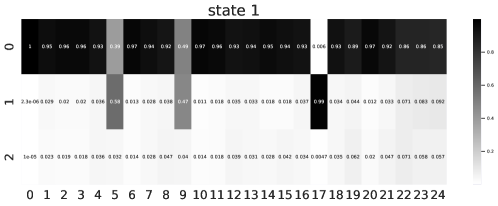
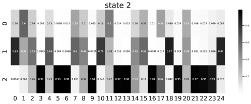
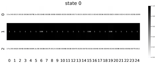
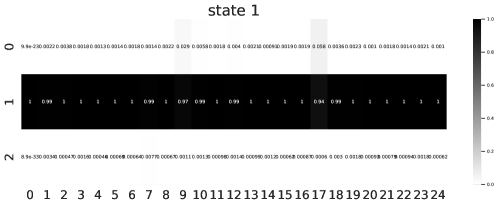
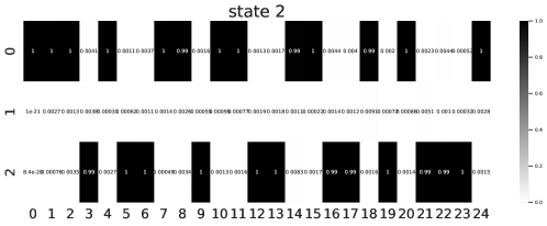
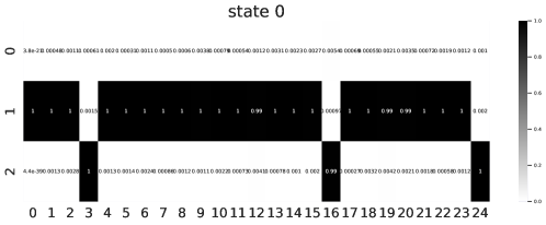
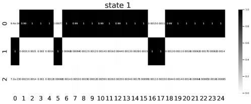
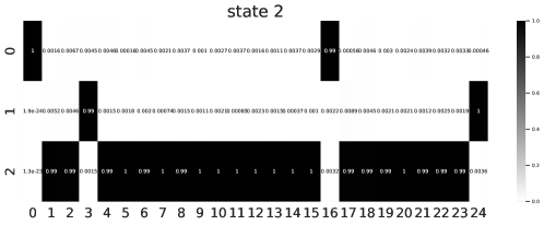
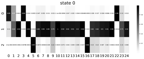
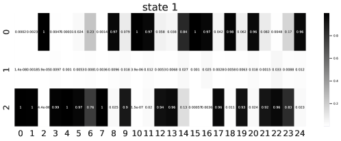
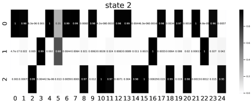
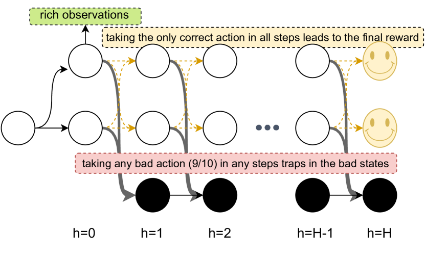
In this section we empirically study the following questions: i) the effectiveness of pretraining with RepTransfer, under the linear span and feature/observation coverage assumptions. ii) the hardness of representational transfer under the linear span assumption without the generative model access. Our experiments are under the Block MDP setting, with the challenging Rich Observation Combination Lock (comblock) benchmark (Fig. 1(a)). We design two sets of experiments to investigate the above questions respectively. We defer the details of the experiments in Appendix J.

Baselines.

We denote Source as the smallest sample complexity of Lsvi-Ucb using learned features from any of the source tasks; O-RepTransfer as RepTransfer with only online access to the source tasks; G-RepTransfer as RepTransfer with generative access to the source tasks; Oracle as learning in the target task with ground truth features; and Target as running Briee (Zhang et al., 2022) — the SOTA Block MDP algorithm, in the target task with no pretraining.

Effectiveness of RepTransfer.

We first analyze the how representational transfer benefits where both feature coverage (Theorem 3.1) and observational coverage (Theorem 4.2) assumptions are met. We use 5 source tasks (horizon $H=25$), with different latent dynamics. To ensure linear span assumption (Assumption 2.2), for each timestep $h$, we make the target latent transition dynamics from one of the sources uniformly at random. For the coverage assumptions, note that for comblock, the feature coverage assumption (Assumption 3.2) is always satisfied. We also guarantee the observational coverage (Assumption 4.1) by equipping all environments with the same emission distribution on a compact observational space. We record the number of episodes in the target environment that each method takes to solve the target environment in Table. 1(b). We first observe that RepTransfer with either online or generative access can solve the target task (since. Assumption 4.1 holds). Second, we observe that directly applying the learned feature from any single source task does not suffice to solve the target environment. This is because the representation learned from a single source task may collapse two latent states into a single one during encoding (e.g., if two latent states at the same time step have exactly identical latent transitions). Third, the result shows that RepTransfer saves order of magnitude of target samples compared with training in the target environment from scratch using the SOTA Block MDPs algorithm BRIEE. This set of results verifies the empirical benefits of representation learning from multiple tasks, i.e., resolves ambiguity and speeds up downstream task learning.

Hardness without the generative access.

In this section, following the intuition of our lower bound (Theorem 4.1), we construct a setting where the supports of the emission distributions from each task are completely disjoint, while the emission distribution in the target task is a mixture of all source emissions and the latent dynamics are identical across tasks. Hence the latent coverage (Assumption 2.2) holds while observational coverage (Assumption 4.1) fails. So we expect that an algorithm without generative access to source tasks will fail based on Theorem 4.1. We record the number of target episodes for each method to solve the target task in Table. 1(b). We observe that indeed the online version fails while the generative version still succeeds. This ablation verifies that source generative model access is needed without the observational coverage.

6 Conclusion

We study representational transfer among low rank MDPs which share the same unknown representation. Under a reasonably flexible linear span task relatedness assumption, we propose an algorithm that provably transfers the representation learned from source tasks to the target task. The regret in target task matches the bound obtained with oracle access to the true representation, using only polynomial number of samples from source tasks. Our approach relies on the generative model access in source tasks, which we prove is not avoidable in the worst case under the linear span assumption. To complement the lower bound, we propose a stronger assumption on the conditions of the reachability in raw states, under which online access to source tasks suffices for provably efficient representation transfer. Finding modalities other than generative access which avoid the lower bound, and a more extensive empirical evaluation beyond the proof-of-concept experiments here are important directions for future research

Appendices

Appendix A Notations

Table 2: List of Notations

${\mathcal{S}},\mathcal{A},A$	State and action spaces, and $A=|\mathcal{A}|$.
$\Delta(S)$	The set of distributions supported by $S$.
$\lambda_{\min}(A)$	Smallest eigenvalue of matrix $A$.
$e_{j}$	One-hot encoding of $j$, i.e. $0$ at each index except the one corresponding to $j$.
	Length of vector implied from context.
$(x)_{\leq y}$	$\min\{x,y\}$.
$H$	Episode length of MDPs, a.k.a. time horizon. We index steps as $h=0,1,...,H-1$.
$K$	The number of source tasks.
$d$	dimension of the low-rank MDP, i.e. dimension of $\phi^{\star}$.
$P^{\star}_{k;h}$	Ground truth transition at time $h$ for source task $k$.
$P^{\star}_{\text{target};h}$	Ground truth transition at time $h$ for target task.
$r_{\text{target};h}$	Reward function of the target task.
$\mathbb{E}_{\pi,P}\left[\cdot\right]$	Expectation under the distribution of trajectories when $\pi$ is executed in $P$.
	We sometimes omit $P$ when the MDP is clear from context.
$d^{\pi}_{P;h}$	Occupancy distribution of $\pi$ under transitions $P$ at time $h$.
$d^{\pi}_{k;h}$	Occupancy distribution for the $k$-th task, i.e. $d^{\pi}_{P^{\star}_{k};h}$.
$\phi_{h}^{\star}(s,a)$	Embedding function for $(s,a)$ at time $h$.
$\Phi_{h}$	Realizable function class for $\phi_{h}^{\star}$.
$|\Phi|$	Defined as $\max_{h}|\Phi_{h}|$.
$\mu_{k;h}^{\star}(s^{\prime})$	Emission embedding function for $s^{\prime}$ at time $h$ for environment $k$.
$\Upsilon_{k;h}$	Realizable function class for $\mu_{k;h}^{\star}$.
$|\Upsilon|$	Defined as $\max_{k;h}|\Upsilon_{k,h}|$.
$\alpha_{\max}$	$\max_{h;k,s^{\prime}\in{\mathcal{S}}}|\alpha_{k;h}(s^{\prime})|$ (based on Assumption 2.2).
$\bar{\alpha}$	$\max_{h}\sum_{k=1}^{K}\max_{s^{\prime}\in{\mathcal{S}}}|\alpha_{k;h}(s^{\prime})|$ (based on Assumption 2.2).
$\psi$	Feature reachability in the source task (Assumption 3.2).
$\psi_{raw}$	Raw states reachability parameter (Assumption 4.1)

Appendix B Omitted Algorithms

Algorithm 3 RewardFree Rep-UCB

1:  Input: Regularizer $\lambda_{n}$, bonus scaling $\alpha_{n}$, model class $\mathcal{M}=\Phi\times\Upsilon$, number of episodes $N$.

2:  Initialize $\widehat{\pi}_{0}$ as random and $\mathcal{D}_{h,0},\mathcal{D}_{h,0}^{\prime}=\emptyset$.

3:  for episode $n=1,2,...,N$ do

4:     Data collection from $\widehat{\pi}_{n-1}$: for $h=1,2,...,H-1$,

$$s\sim d^{\widehat{\pi}_{n-1}}_{h},a\sim\operatorname{Unif}(\mathcal{A}),s^{\prime}\sim P^{\star}_{h}(s,a);$$

$$\widetilde{s}\sim d^{\widehat{\pi}_{n-1}}_{h-1},\widetilde{a}\sim\operatorname{Unif}(\mathcal{A}),\widetilde{s}^{\prime}\sim P^{\star}_{h-1}(\widetilde{s},\widetilde{a}),\widetilde{a}^{\prime}\sim\operatorname{Unif}(\mathcal{A}),\widetilde{s}^{\prime\prime}\sim P^{\star}_{h}(\widetilde{s}^{\prime},\widetilde{a}^{\prime});$$

$$\mathcal{D}_{h,n}=\mathcal{D}_{h,n-1}\cup\left\{(s,a,s^{\prime})\right\},\mathcal{D}_{h,n}^{\prime}=\mathcal{D}_{h,n-1}^{\prime}\cup\left\{(\widetilde{s}^{\prime},\widetilde{a}^{\prime},\widetilde{s}^{\prime\prime})\right\}.$$

For $h=0$, only collect $\mathcal{D}_{0,n}$.

5:     Learn model via MLE: for all $h=0,1,...,H-1$,

$$\widehat{P}_{h,n}=(\widehat{\phi}_{h,n},\widehat{\mu}_{h,n})=\mathop{\mathrm{argmax}}_{\phi_{h},\mu_{h}\in\mathcal{M}_{h}}\mathbb{E}_{\mathcal{D}_{h,n}\cup\mathcal{D}_{h,n}^{\prime}}\left[\log\phi_{h}(s,a)^{T}\mu_{h}(s^{\prime})\right].$$

6:     Update exploration bonus: for all $h=0,1,...,H-1$,

$$\widehat{b}_{h,n}(s,a)=\alpha_{n}\left\lVert\widehat{\phi}_{h,n}(s,a)\right\rVert_{\widehat{\Sigma}_{h,n}^{-1}}$$

$$\widehat{\Sigma}_{h,n}=\sum_{(s,a,\_)\in\mathcal{D}_{h,n}}\widehat{\phi}_{h,n}(s,a)\widehat{\phi}_{h,n}(s,a)^{T}+\lambda_{n}I.$$

7:     Learn policy $\widehat{\pi}_{n}=\mathop{\mathrm{argmax}}_{\pi}V^{\pi}_{\widehat{P}_{n},\widehat{b}_{n}}$ and let $\widehat{V}_{n}$ be its value.

8:  end for

9:  Let $\widehat{n}=\mathop{\mathrm{argmin}}_{n\geq N/2}\widehat{V}_{n}$.

10:  Output: $\widehat{n},\widehat{P}_{\widehat{n}}$.

Algorithm 4 Transfer learning with online access

Pre-Training Phase
Input: num. Lsvi-Ucb episodes $N_{\textsc{Lsvi-Ucb}}$, num. model-learning episodes $N_{\textsc{RewardFree}}$, size of cross-sampled datasets $n$, failure probability $\delta$.

1:  for source task $k=1,...,K-1$ do

2:     Find policy cover $\pi_{k}=$RewardFree$(P_{k}^{\star},N_{\textsc{Lsvi-Ucb}},N_{\textsc{RewardFree}},\delta)$. (Algorithm 1)

3:  end for

4:  for source task $k=1,...,K-1$ do

5:     For each $h\in[0:H-1]$, sample $\mathcal{D}_{k}$ as $n$ i.i.d. $(s_{h},a_{h},s_{h+1})$ tuples from $\pi_{k}$.

6:  end for

7:  For each $h\in[0:H-1]$, learn features with MLE,

$$\widehat{\phi}_{h},\widehat{\mu}_{1:K}=\mathop{\mathrm{argmax}}_{\phi\in\Phi,\mu_{k}\in\Upsilon_{k}}\sum_{k\in[K]}\mathbb{E}_{\mathcal{D}_{k;h}}\left[\log\phi(s,a)^{\top}\mu_{k}(s^{\prime})\right].$$

Deployment Phase

Additional Input: number of deployment episodes $T$.

1:  Set $\beta=H\sqrt{d}+\bar{\alpha}dH\sqrt{\log(dHT/\delta)}$.

2:  Run $\textsc{Lsvi-Ucb}\left(\{\widehat{\phi}_{h}\}_{h=0}^{H-1},r=r_{K},T,\beta\right)$ in the target task $P_{\text{target}}^{\star}$ (Algorithm 5).

Let $(x)_{\leq y}$ refer to the clamping operator, i.e. $(x)_{\leq y}=\min\{x,y\}$. Let $M_{V}$ be the maximum possible value in the MDP with the given reward function.

Algorithm 5 Lsvi-Ucb

1:  Input: Features $\{\widehat{\phi}_{h}\}_{h=0,1,...,H-1}$, reward $\{r_{h}\}_{h=0,1,...,H-1}$, number of episodes $N$, bonus scaling parameter $\beta$, UniformActions = False.

2:  for episode $e=1,2,...,N$ do

3:     Initialize $\widehat{V}_{H,e}(s)=0,\forall s$

4:     for step $h=H-1,H-2...,0$ do

5:        Learn best predictor for $\widehat{V}_{h+1}^{e}$,

$$\Lambda_{h,e}=\sum_{k=1}^{e-1}\widehat{\phi}_{h}(s_{h}^{k},a_{h}^{k})\widehat{\phi}_{h}(s_{h}^{k},a_{h}^{k})^{\top}+I,$$

$$\widehat{w}_{h,e}=\Lambda_{h,e}^{-1}\sum_{k=1}^{e-1}\widehat{\phi}_{h}(s_{h}^{k},a_{h}^{k})\widehat{V}_{h+1,e}(s^{k}_{h+1}).$$

6:        Set bonus and value functions,

$$b_{h,e}(s,a)=\left\lVert\widehat{\phi}_{h}(s,a)\right\rVert_{\Lambda_{h,e}^{-1}},$$

$$\widehat{Q}_{h,e}(s,a)=\widehat{w}_{h,e}^{\top}\widehat{\phi}_{h}(s,a)+r_{h}(s,a)+\beta b_{h,e}(s,a),$$

$$\widehat{V}_{h,e}(s)=\left(\max_{a}\left\{\widehat{Q}_{h,e}(s,a)\right\}\right)_{\leq M_{V}}.$$

7:        Set $\pi_{h}^{e}(s)=\mathop{\mathrm{argmax}}_{a}\widehat{Q}_{h,e}(s,a)$.

8:     end for

9:     Execute $\pi^{e}$ to collect a trajectory $(s^{e}_{h},a_{h}^{e})_{h=0}^{H-1}$.

10:     If UniformActions = True, discard $a_{h}^{e}$ and draw freshly sampled uniform actions independently for all $h$, i.e. $a_{h}^{e}\sim\operatorname{Unif}(\mathcal{A})$.

11:  end for

12:  Return: uniform mixture $\rho=\text{Uniform}(\{\pi^{e}\}_{e=1}^{N})$.

Appendix C More discussion on related works

C.1 Empirical works in transfer learning

The idea of learning transferable representation has been extensively explored in the empirical literature. Here we don’t intend to provide a comprehensive survey of all existing works on this topic. Instead, we discuss a few representative approach that may be of interest.
Towards transfer learning across different environments, progressive neural network (Rusu et al., 2016) is among the first neural-based attempt to learning a transferable representation for a sequence of downstream tasks that tries to overcome the challenge of catastrophic forgetting. It maintains the learned neural models for all previous tasks and introduce additional connections between the network of the current tasks to those of prior tasks to allow information reuse. However, a drawback common to such an approach is that the network size grows linearly with the number of tasks. Other approaches include directly learning a multi-task policy that can perform well on a set of source tasks, with the hope that it will generalize to future tasks (Parisotto et al., 2015). Such an approach requires the tasks to be similar in their optimal policy, which is a much stronger assumption than ours.
Slightly off-topic are the works about “transfer learning” inside the same environment but across different reward functions, which is more restricted than the setting considered in this paper. Several prior works design representation learning algorithms that aim to learn a representation that generalize across multiple reward function/goals (Dayan, 1993; Barreto et al., 2017; Touati and Ollivier, 2021; Blier et al., 2021). These are related to the RewardFree Rep-UCB we developped in Section E. The key difference is that we concern representation learning along with efficient exploration to derive an end-to-end polynomial sample complexity bound. These prior works do not consider exploration and do not come with provable sample complexity bounds. We refer interested readers to a recent survey (Zhu et al., 2020) for a comprehensive discussion of other empirical approaches.

C.2 Comparison to Lu et al. (2021)

In the prior work of Lu et al. (2021), which also studies transfer learning in low-rank MDPs with nonlinear function approximations, they need to make the following assumptions:

1. shared representation (identical to our Assumption 2.1).

2. task diversity (similar to our Assumption 2.2).

3. generative model access to both the source and the target tasks. In contrast, we only require generative model access to the source tasks and allow online learning in the target task.

4. a somewhat strong coverage assumption saying that the data covariance matrix (under the generative data distribution) between arbitrary pairs of features $\phi,\phi^{\prime}\in\Phi$ must be full rank. In contrast, our analysis only requires coverage in the true feature $\phi^{\star}$ in the source tasks.

5. the existence of an ideal distribution q on which the learned representation can extrapolate. We do not require an assumption of a similar nature. Instead, we show that the data collected from our strategic reward-free exploration phase suffices for successful transfer.

6. the uniqueness for each $\phi$ in the sense of linear-transform equivalence. Two representation functions $\phi$ and $\phi^{\prime}$ can yield similar estimation result if and only if they differ by just an invertible linear transformation. In contrast, we do not make any additional structural assumptions on the function class $\Phi$ beyond realizability.

In summary, our work present a theoretical framework that permits successful representation transfer based on significantly weaker assumptions. We believe that this is a solid step towards understanding transfer learning in RL.

C.3 Comparison to Cheng et al. (2022)

Cheng et al. (2022) studies representational transfer in low-rank MDPs, with not only a weaker notion of task relatedness (with global coefficients in the linear span) but also stronger assumptions. Particularly, we restate the following strong assumption from Cheng et al. (2022, Assumption 5.3).

Assumption C.1.

For any two different models in the model class $\Phi\times\Psi$, say $P^{1}(s^{\prime}|s,a)=\langle\phi^{1}(s,a),\mu^{1}(s^{\prime})\rangle$ and $P^{2}(s^{\prime}|s,a)=\langle\phi^{2}(s,a),\mu^{2}(s^{\prime})\rangle$, there exists a constant $C_{R}$ such that for all $(s,a)\in{\mathcal{S}}\times\mathcal{A}$ and $h\in[H]$,

$$\|P^{1}(\cdot|s,a)-P^{2}(\cdot|s,a)\|_{TV}\leq C_{R}\mathbb{E}_{(s,a)\sim\mathcal{U}({\mathcal{S}},\mathcal{A})}\|P^{1}(\cdot|s,a)-P^{2}(\cdot|s,a)\|_{TV}$$

This assumption ensures that the point-wise TV error is bounded, as long as the population-level TV error is bounded. Cheng et al. (2022) used this to transfer the MLE error from the source tasks to the target task. This type of assumption is strong in the sense that we typically expect $C_{R}$ to scale with $|{\mathcal{S}}|$. In contrast, our analysis (Lemma G.1) shows that this assumption is in fact not necessary, even assuming online access only to source tasks. The generative access to source task studied here, which enables transfer under weaker reachability assumptions is not studied in their work.

It is worth noting that Cheng et al. (2022) also study offline RL in the target task which we do not cover, while we mainly focus on the setting of generative models in the source tasks and demonstrating a more complete picture by proving generative model access in source tasks is needed without additional assumptions. Comparing to (Cheng et al., 2022), we also further implement and perform experimental evaluations of our algorithm.

C.4 Works in multi-task learning

Multi-task and Transfer Learning in Supervised Learning. The theoretical benefit of representation learning are well studied under conditions such as the i.i.d. task assumption (Maurer et al., 2016) and the diversity assumption (Du et al., 2020; Tripuraneni et al., 2020). Many works below successfully adopt the frameworks and assumptions to sequential decision making problems.

Multi-task and Transfer Learning in Bandit and small-size MDPs. Several recent works study multi-task linear bandits with linear representations ($\phi(s)=A\,s$ with unknown $A$) (Hu et al., 2021; Yang et al., 2020, 2022). The techniques developed in these works crucially rely on the linear structure and can not be applied to nonlinear function classes. Lazaric et al. (2013) study spectral techniques for online sequential transfer learning. Brunskill and Li (2013) study multi-task RL under a fixed distribution over finitely many MDPs, while Brunskill and Li (2014) consider transfer in semi-MDPs by learning options. Lecarpentier et al. (2021) consider lifelong learning in Lipschitz MDP. All these works consider small size tabular models while we focus on large-scale MDPs.

Multi-task and Transfer Learning in RL via representation learning. Beyond tabular MDPs, Arora et al. (2020) and D’Eramo et al. (2019) show benefits of representation learning in imitation learning and planning, but do not address exploration. Lu et al. (2021) study transfer learning in low-rank MDPs with general nonlinear representations, but make a generative model assumption on both the source tasks and the target task, along with other distributional and structural assumptions. We do not require generative access to the target task and make much weaker structural assumptions on the source-target relatedness. Recently and independently, Cheng et al. (2022) also studied transfer learning in low-rank MDPs in the online learning setting, identical to the setting we study in Section 4. However, their analysis relies on an additional assumption that bounds the point-wise TV error with the population TV error, which we show is in fact not necessary.

Efficient Representation Learning in RL. Even in the single task setting, efficient representation learning is an active area witnessing recent advances with exploration (Agarwal et al., 2020; Modi et al., 2021; Uehara et al., 2021; Zhang et al., 2022) or without (Ren et al., 2021). Other papers study feature selection (e.g. Farahmand and Szepesvári, 2011; Jiang et al., 2015; Pacchiano et al., 2020; Cutkosky et al., 2021; Lee et al., 2021; Zhang et al., 2021) or sparse models (Hao et al., 2021a, b).

Appendix D Impossibility Results

Here, we present an interesting result showing that the above assumptions we make are so weak that they do not even permit efficient transfer in supervised learning:

Theorem D.1 (Counter-example in supervised learning).

Assume that we want to perform conditional density estimation, where $P^{\star}_{k}(y|x)=\phi^{\star}(x)^{\top}\mu_{k}^{\star}(y)$. Under Assumption 2.1 (shared representation) and Assumption 2.2 (linear span), and assume that in each source task, one have access to a data generating distribution $\rho_{k}(x)$ such that $\lambda_{\min}\mathbb{E}_{\rho_{k}}[\phi^{\star}(x)\phi^{\star}(x)^{\top}]\geq\psi$ (reachability). No algorithm can consistently achieve $\mathbb{E}_{\rho_{K}}[\|\hat{P}^{\star}_{\text{target}}(y|x)-P^{\star}_{\text{target}}(y|x)\|_{TV}]\leq 1/2$ on the target task using the feature learned from the source tasks with probability more than $1/2$.

Proof of Theorem D.1.

Consider the following example. $X=\mathbb{R}^{2}$ and we have the following 3 sets.

$${\mathcal{S}}_{1}= \;B_{1/2}((-1,-1))$$

$${\mathcal{S}}_{2}= \;B_{1/2}((-2,-2))$$

$${\mathcal{S}}_{3}= \;B_{1/2}((0,1))$$

where $B_{a}((x,y))$ stands for the ball with radius $a$ centered at $(x,y)$. These will be the support of 3 tasks: task 1 and 2 are two source tasks, task 3 is the target task. Let’s assume that $P^{\star}_{k}(x)$ are uniform distribution on ${\mathcal{S}}_{k}$.

Suppose that the feature class $\Phi$ only contains two functions:

$$\phi_{1}:\{x_{1}\leq 0\And x_{2}\geq x_{1}\}\rightarrow(1,0)\text{, and $(0,1)$ otherwise}$$

$$\phi_{2}:\{x_{2}\leq 0\And x_{1}\geq x_{2}\}\rightarrow(0,1)\text{, and $(1,0)$ otherwise}$$

That is, the feature maps from $\mathbb{R}^{2}$ to the set of binary encoding of dimension 2, i.e. $\{(1,0),(0,1)\}$. We further assume that $\mu^{\star}_{k}=(p_{1}(y),p_{2}(y))$ for some distributions $p_{1},p_{2}$, which is identical for all task $k$, where $\|p_{1},p_{2}\|_{TV}=1$. We also assume that $\mu^{\star}_{k}$ is known to the learner a prior, i.e. $\Upsilon_{k}=\{\mu^{\star}_{k}\}$ for all $k\in[K]$, so all the learner needs to do is to pick the correct $\phi$ out of two candidates.

Given the above setup, it’s easy to verify that both Assumption 2.1 and Assumption 2.2 are satisfied, because the decision boundary of both $\phi_{1}$ and $\phi_{2}$ passes through the support of the source tasks, and all $\mu^{\star}_{k}$’s are identical. However, $\phi_{1}$ and $\phi_{2}$ are equivalent in ${\mathcal{S}}_{1}$ and ${\mathcal{S}}_{2}$ in terms of their representation power, therefore no algorithm can always pick the correct feature function with probability more than $1/2$, regardless of the number of samples. Suppose $\phi_{1}$ is the true feature and the algorithm incorrectly chooses $\phi_{2}$. Then, for $x\in S_{3}\bigcap\{x_{1}\geq 0\}$ which has probability mass $1/2$, $\hat{P}_{3}(y|x)=p_{2}$ whereas $P^{\star}_{3}(y|x)=p_{1}$. Thus, the expected total variation distance between $\hat{P}_{\text{target}}$ and $P^{\star}_{\text{target}}$ is $1/2$. ∎

The above construction shows that our assumption are not sufficient to permit reliable representation transfer, even in the supervised learning setting. Yet, surprisingly, these assumptions are sufficient in the RL setting, implying somehow that transfer learning in RL in easier than transfer learning in SL. To understand this phenomenon, observe that in RL, the marginal distribution on $(s,a)$ is not independent from the conditional density $P(s^{\prime}|s,a)$ we desire to estimate. In particular, if one collects data in the source tasks in an online fashion via running a policy, $\rho(s,a)$ is structurally restricted to be an occupancy distribution generated by the ground-truth transition $P^{\star}(s^{\prime}|s,a)$. Such a connection can only exist in Markov chains, and our analysis elegantly utilizes this additional structure to establish the soundness of the learned representation. Also note, crucially, that we never learn a representation to capture $d_{0}$, which would suffer from similar issues as the supervised learning setting, but is not necessary for sample-efficient RL.

Next, we prove the impossibility result in Theorem 4.1, restated below as Theorem D.3. This result shows that one can not achieve online learning in the source tasks without significantly stronger assumptions such as Assumption 4.1. Before that, we provide a preliminary version, showing that the learned $\hat{\phi}$ is not sufficient to fit the transition model in the target task, which motivates the construction in Theorem D.3.

Theorem D.2 (Impossibility Result: Model Learning).

Let $\mathcal{M}=\{(P_{1},...,P_{K},P_{\text{target}})\}$ be a set of $K+1$ tasks that satisfies

1. all tasks are Block MDPs;

2. all tasks satisfy Assumption 3.2 and Assumption 2.2;

3. the latent dynamics are exactly the same for all source and target tasks.

For any pre-training algorithm $\mathcal{A}$, there exists $(P_{1},...,P_{K},P_{\text{target}})\in\mathcal{M}$ and an occupancy distribution $\rho_{\text{target}}$ on the target task, such that with probability at least $1/2$, $\mathcal{A}$ will output a feature $\hat{\phi}$ and for any $\mu$

$$\mathbb{E}_{\rho_{\text{target}}}\|\hat{\phi}(s,a)^{\top}\mu(\cdot)-P^{\star}_{\text{target}}(\cdot|s,a)\|_{TV}\geq 1/2.$$

Proof of Theorem D.2.

Consider a tabular MDP with 2 latent states $z_{1},z_{2}$ and an observation state space ${\mathcal{S}}=R_{1}\bigcup R_{2}\bigcup B_{1}\bigcup B_{2}$, where in task 1 one can only observe $R_{1}\bigcup R_{2}$ and in task 2 one can only observe $B_{1}\bigcup B_{2}$. Correspondingly, $o_{1}(s|z)$ is only supported on $R_{1}\bigcup R_{2}$ (i.e., $o_{1}(R_{i}|z_{i})=1$) and similar for task 2. Let the latent state transition be such that $P(z_{1}|z_{1},a)=1$ and $P(z_{2}|z_{2},a)=1$, i.e. only self-transition regardless of the actions.

Now, consider a 2-element feature class $\Psi=\{\psi_{1},\psi_{2}\}$ such that

$$\psi_{1}= \;\{R_{1}\rightarrow 1,R_{2}\rightarrow 2,B_{1}\rightarrow 1,B_{2}\rightarrow 2\}$$

$$\psi_{2}= \;\{R_{1}\rightarrow 1,R_{2}\rightarrow 2,B_{1}\rightarrow 2,B_{2}\rightarrow 1\}$$

Denote $\phi_{i}(s,a)=e_{(\psi_{i}(s),a)}$ for $i\in[1,2]$. Consider for each task $k$, a 2-element $\Upsilon_{k}$ class in the form of $\Upsilon_{k}=\{(o_{k}(s|z_{1}),o_{k}(s|z_{2})),(o_{k}(s|z_{2}),o_{k}(s|z_{1}))\}$.

Notice that $\phi_{1}$ and $\phi_{2}$ are merely permutations of one another and so given any single task data, the two hypothesis will not be distinguishable by any means. Therefore, for any algorithm, there is at least probability $1/2$ that it will choose the wrong hypothesis if the ground truth $\phi^{\star}$ is sampled between $\phi_{1}$ and $\phi_{2}$ uniformly at random. Suppose $\phi_{1}$ is the correct hypothesis and $\phi_{2}$ is the one that the algorithm picks (i.e., $\hat{\phi}=\phi_{2}$). Let task 3 be such that any state emits to $R_{1}\bigcup R_{2}$ and $B_{1}\bigcup B_{2}$ each with probability $1/2$ (i.e., $o_{3}(R_{i}|z_{i})=o_{3}(B_{i}|z_{i})=0.5$). This construction satisfies Assumption 3.2 and Assumption 2.2.

Then, within task 3, one would encounter observations from both $R_{1}$ and $B_{2}$ which should be mapped to latent state $z_{1}$ and $z_{2}$ respectively by the true decoder $\phi_{1}$, but are instead both mapped to latent state $z_{1}$ by the learned decoder $\phi_{2}$, and thus $z_{1}$ and $z_{2}$ become indistinguishable. Suppose $\rho_{\text{target}}(z_{1})=\rho_{\text{target}}(z_{2})=1/2$, then

$$\;\mathbb{E}_{\rho_{\text{target}}}[\|\hat{\phi}(s,a)^{\top}\mu(\cdot)-P^{\star}(\cdot|s,a)\|_{TV}]$$

$$\;=\frac{1}{4}\|\hat{\phi}(R_{1})^{\top}\mu(\cdot)-\phi(R_{1})^{\star\top}\mu^{\star}(\cdot)\|_{TV}+\frac{1}{4}\|\hat{\phi}(B_{1})^{\top}\mu(\cdot)-\phi(B_{1})^{\star\top}\mu^{\star}(\cdot)\|_{TV}$$

$$\;\quad\quad+\frac{1}{4}\|\hat{\phi}(R_{2})^{\top}\mu(\cdot)-\phi(R_{2})^{\star\top}\mu^{\star}(\cdot)\|_{TV}+\frac{1}{4}\|\hat{\phi}(B_{2})^{\top}\mu(\cdot)-\phi(B_{2})^{\star\top}\mu^{\star}(\cdot)\|_{TV}$$

$$\;=\|o_{1}-o_{1}^{\star}\|_{TV}/4+\|o_{2}-o_{1}^{\star}\|_{TV}/4+\|o_{2}-o_{2}^{\star}\|_{TV}/4+\|o_{1}-o_{2}^{\star}\|_{TV}/4$$

$$\;\geq\frac{1}{4}\|o_{1}^{\star}-o_{2}^{\star}\|_{TV}+\frac{1}{4}\|o_{1}^{\star}-o_{2}^{\star}\|_{TV}$$

$$\;=\frac{1}{2},$$

where the last second inequality uses triangle inequality, and the last equality comes from the fact that $o_{3}(\cdot|z_{1})$ and $o_{3}(\cdot|z_{2})$ have disjoint support which implies that $\|p_{1}^{\star}-p_{2}^{\star}\|_{TV}=1$. ∎

Now, we are ready to restate and prove Theorem 4.1.

Theorem D.3 (Impossibility Result: Optimal Policy Identification).

Let $\mathcal{M}=\{(P_{1},...,P_{K},P_{\text{target}})\}$ be a set of $K+1$ tasks that satisfies

1. all tasks are Block MDPs;

2. all tasks satisfy Assumption 3.2 and Assumption 2.2;

3. the latent dynamics are exactly the same for all source and target tasks.

For any pre-training algorithm $\mathcal{A}$, there exists $(P_{1},...,P_{K},P_{\text{target}})\in\mathcal{M}$, such that with probability at least $1/2$, $\mathcal{A}$ will output a feature $\hat{\phi}$, such that for any policy taking the functional form of $\pi(s)=f\left(\{\hat{\phi}(s,a)\}_{a\in\mathcal{A}},\{r(s,a)\}_{a\in\mathcal{A}}\right)$, we have

$$V^{\star}-V^{\pi}\geq 1/2.$$

Proof of Theorem D.3.

Consider a tabular MDP with $H=2$, two latent states $z_{1},z_{2}$ for $h=1$ and two latent states $z_{3},z_{4}$ for $h=2$.

• For $h=1$, let there be two actions $a_{1},a_{2}$. Let the observation state space be ${\mathcal{S}}=R_{1}\bigcup R_{2}\bigcup B_{1}\bigcup B_{2}$, where in task 1 one can only observe $R_{1}\bigcup R_{2}$ and in task 2 one can only observe $B_{1}\bigcup B_{2}$. Correspondingly, $o_{1}(s|z)$ is only supported on $R_{1}\bigcup R_{2}$ (i.e., $o_{1}(R_{i}|z_{i})=1$) and similar for task 2. Let the latent state transition be such that $P(z_{3}|z_{1},a_{1})=P(z_{3}|z_{2},a_{2})=1$, and $P(z_{4}|z_{1},a_{2})=P(z_{4}|z_{2},a_{1})=1$. All rewards are $0$ for $h=1$.

• For $h=2$, in state $z_{3}$, all actions have reward $1$, and in state $z_{4}$ all actions have reward $0$.

• The initial state distribution is $d_{0}(z_{1})=d_{0}(z_{2})=1/2$.

Now, consider a 2-element feature class $\Psi=\{\psi_{1},\psi_{2}\}$ for $h=1$, such that

$$\psi_{1}= \;\{R_{1}\rightarrow 1,R_{2}\rightarrow 2,B_{1}\rightarrow 1,B_{2}\rightarrow 2\}$$

$$\psi_{2}= \;\{R_{1}\rightarrow 1,R_{2}\rightarrow 2,B_{1}\rightarrow 2,B_{2}\rightarrow 1\}$$

Denote $\phi_{i}(s,a)=e_{(\psi_{i}(s),a)}$ for $i\in[1,2]$. In addition, define $\Upsilon=\{\mu_{1},\mu_{2}\}$ where

$$\mu_{1}= \;\{z_{3}\rightarrow(1,0),z_{4}\rightarrow(0,1)\}$$

$$\mu_{2}= \;\{z_{4}\rightarrow(1,0),z_{3}\rightarrow(0,1)\}$$

Notice that $\phi_{1}$ and $\phi_{2}$ are merely permutations of one another and so given any single task data, the two hypothesis will not be distinguishable by any means. Therefore, for any algorithm, there is at least probability $1/2$ that it will choose the wrong hypothesis. Suppose $\phi_{1}$ is the correct hypothesis and $\phi_{2}$ is the one that the algorithm picks (i.e., $\hat{\phi}=\phi_{2}$). Let task 3 be such that any state emits to $R_{1}\bigcup R_{2}$ and $B_{1}\bigcup B_{2}$ each with probability $1/2$ (i.e., $o_{3}(R_{i}|z_{i})=o_{3}(B_{i}|z_{i})=0.5$). This construction satisfies Assumption 3.2 and Assumption 2.2.

Then, for any policy that only make decision based on $\hat{\phi}(s,a)$ and $r(s,a)$, $\pi$ would output the same action for observations in $R_{1}$ and $B_{2}$, or for $B_{1}$ and $R_{2}$. However, notice that the optimal policy, which would try to go to $z_{3}$ from either $z_{1}$ or $z_{2}$, will pick $a_{1}$ at $R_{1}$ and $B_{1}$ while picking $a_{2}$ at $R_{2}$ and $B_{2}$, which means that the optimal policy will not agree on $R_{1}$ and $B_{2}$, and it also will not agree on $R_{2}$ and $B_{1}$. Thus clearly, no such policy as defined above is capable of capturing the optimal policy. From the reward perspective, notice that $d^{\pi}(z_{1})=d^{\pi}(z_{2})=1/2$ and $d^{\pi}(R_{1})=d^{\pi}(R_{2})=d^{\pi}(B_{1})=d^{\pi}(B_{1})=1/4$. Since $\pi(R_{1})=\pi(B_{2})$, the agent will only be able to collect reward at one of the $R_{1}$ and $B_{2}$ (but not at both). Similarly, since $\pi(R_{2})=\pi(B_{1})$, the agent will only be able to collect reward at one of the $R_{2}$ and $B_{1}$ by reaching $z_{3}$ (but not at both). This means that $\pi$ will have average reward $1/2$. Since the optimal policy will be able to collect reward at all $R_{1},R_{2},B_{1},B_{2}$, it will have average reward $1$. This concludes the proof. ∎

Theorem D.2 and Theorem D.3 show that it’s impossible to allow online learning in the source tasks without much stronger assumptions. In our paper, we show that our Assumption 4.1, which ensures reachability in the raw states, is sufficient to establish an end-to-ending online transfer learning result. However, it is unclear if Assumption 4.1 is necessary for online learning. We leave this as an important direction of future work.

Appendix E Reward-free Rep-UCB

In this section, we adapt the Rep-UCB algorithm (Uehara et al., 2021) for reward-free exploration in a single task. We drop all task subscripts as this section is for a single task only, i.e. think about the task as being each source task. The original Rep-UCB algorithm was for infinite-horizon discounted MDPs, so we modify it to work for our undiscounted and finite-horizon setting. Our goal is to prove that Rep-UCB can learn a model that satisfies strong TV guarantees, i.e. Theorem E.1 and (7). Note that FLAMBE (Agarwal et al., 2020, Theorem 2) can be used for this directly, but at a worse (polynomial) sample complexity. Thus, we do a bit more work to derive a new model-learning algorithm for low-rank MDPs, based on Rep-UCB, that is more sample efficient in the source tasks.

A finite-horizon analysis of Rep-UCB was done in BRIEE (Zhang et al., 2022), so here we just need to replace BRIEE’s RepLearn $\zeta_{n}$ with that of the MLE, which is how we learn $\widehat{\phi}$ and $\widehat{\mu}$, as in Rep-UCB. Recall the notation of (Zhang et al., 2022),

$$\rho_{h,n}(s,a)=\frac{1}{n}\sum_{i=0}^{n-1}d^{\widehat{\pi}_{i}}_{h}(s)\operatorname{Unif}(a)$$

$$\beta_{h,n}(s,a)=\frac{1}{n}\sum_{i=0}^{n-1}\mathbb{E}_{\widetilde{s}\sim d^{\widehat{\pi}_{i}}_{h-1},\widetilde{a}\sim\operatorname{Unif}(\mathcal{A})}\left[P_{h}^{\star}(s\mid\widetilde{s},\widetilde{a})\operatorname{Unif}(a)\right]$$

$$\gamma_{h,n}(s,a)=\frac{1}{n}\sum_{i=0}^{n-1}d^{\widehat{\pi}_{i}}_{h}(s,a)$$

$$\Sigma_{\rho,\phi,n}=n\mathbb{E}_{\rho}\left[\phi(s,a)\phi(s,a)^{T}\right]+\lambda_{n}I.$$

By using MLE (Uehara et al., 2021, Lemma 18) to learn models, with probability at least $1-\delta$, for any $n=1,2,...,N$ and $h=0,1,...,H-1$, we have

$$\max\left\{\mathbb{E}_{\rho_{h,n}}\left\lVert\widehat{P}_{h,n}(s,a)-P^{\star}_{h}(s,a)\right\rVert_{TV}^{2},\mathbb{E}_{\beta_{h,n}}\left\lVert\widehat{P}_{h,n}(s,a)-P^{\star}_{h}(s,a)\right\rVert_{TV}^{2}\right\}\leq\zeta_{n},$$ (5)

where

$$\zeta_{n}=\mathcal{O}\left(\frac{\log\left(|\mathcal{M}|nH/\delta\right)}{n}\right),$$

and $|\mathcal{M}|=\max_{h\in[H]}|\Phi_{h}||\Upsilon_{h}|$. We also adopt the same choice of $\alpha_{n},\lambda_{n}$ parameters as BRIEE, which we assume from now on.

$$\lambda_{n}=\Theta\left(d\log(|\mathcal{M}|nH/\delta)\right)$$

$$\alpha_{n}=\Theta\left(\sqrt{n|\mathcal{A}|^{2}\zeta_{n}+\lambda_{n}d}\right).$$

As in Rep-UCB, we posit standard assumptions about realizability and normalization, on the (source) task of interest.

Assumption E.1.

For any $h=0,1,...,H-1$, we have $\phi_{h}^{\star}\in\Phi_{h}$ and $\mu_{h}^{\star}\in\Upsilon_{h}$. For any $\phi\in\Phi_{h}$, $\|\phi(s,a)\|_{2}\leq 1$. For all $\mu\in\Upsilon_{h}$ and any function $g:{\mathcal{S}}\to\mathbb{R}$, we have $\|\int_{s}g(s)\mathrm{d}\mu(s)\|_{2}\leq\|g\|_{\infty}\sqrt{d}$.

Lemma E.1.

Let $r$ be any reward function. Suppose we ran Algorithm 3 with line 7 having reward $r+\widehat{b}_{n}$ instead of just $\widehat{b}_{n}$. Then, for any $\delta\in(0,1)$, w.p. at least $1-\delta$, we have

$$\sum_{n=0}^{N-1}V^{\widehat{\pi}_{n}}_{\widehat{P}_{n},r+\widehat{b}_{n}}-V^{\widehat{\pi}_{n}}_{P^{\star},r}\leq\mathcal{O}\left(H^{2}d^{2}|\mathcal{A}|^{1.5}\sqrt{N\log(|\mathcal{M}|NH/\delta)}\right)$$

Proof.

Start from the third equation of Zhang et al. (2022, Theorem A.4). Following their proof until the last page of their proof, we arrive at the following: for any $n=1,2,...,N$,

$$V^{\widehat{\pi}_{n}}_{\widehat{P}_{n},r+\widehat{b}_{n}}-V^{\widehat{\pi}_{n}}_{P^{\star},r}$$

$$\lesssim\sum_{h=0}^{H-2}\mathbb{E}_{\widetilde{s},\widetilde{a}\sim d^{\widehat{\pi}_{n}}_{P^{\star},h}}\left\lVert\phi^{\star}_{h}(\widetilde{s},\widetilde{a})\right\rVert_{\Sigma_{\gamma_{h,n},\phi^{\star}_{h}}^{-1}}\sqrt{|\mathcal{A}|\alpha_{n}^{2}d+\lambda_{n}d}+\sqrt{|\mathcal{A}|\alpha_{1}^{2}d/n}$$

$$+(2H+1)\sum_{h=0}^{H-2}\mathbb{E}_{\widetilde{s},\widetilde{a}\sim d^{\widehat{\pi}_{n}}_{P^{\star},h}}\left\lVert\phi^{\star}_{h}(\widetilde{s},\widetilde{a})\right\rVert_{\Sigma_{\gamma_{h,n},\phi^{\star}_{h}}^{-1}}\sqrt{n|\mathcal{A}|\zeta_{n}+\lambda_{n}d}+(2H+1)\sqrt{|\mathcal{A}|\zeta_{n}}.$$

By elliptical potential arguments, we have

$$\sum_{n=0}^{N-1}\mathbb{E}_{\widetilde{s},\widetilde{a}\sim d^{\widehat{\pi}_{n}}_{P^{\star},h}}\left\lVert\phi^{\star}_{h}(\widetilde{s},\widetilde{a})\right\rVert_{\Sigma_{\gamma_{h,n},\phi^{\star}_{h}}^{-1}}\leq\sqrt{dN\log\left(1+\frac{N}{d\lambda_{1}}\right)}.$$

Thus, summing over $n$, noting that $n\zeta_{n},\alpha_{n},\lambda_{n}$ are increasing in $n$, we can combine the above to get,

$$\sum_{n=0}^{N-1}V^{\widehat{\pi}_{n}}_{\widehat{P}_{n},r+\widehat{b}_{n}}-V^{\widehat{\pi}_{n}}_{P^{\star},r}$$

$$\lesssim\sqrt{dN\log\left(1+\frac{N}{d\lambda_{1}}\right)}\left(H\sqrt{|\mathcal{A}|\alpha_{N}^{2}d+\lambda_{N}d}+H^{2}\sqrt{N|\mathcal{A}|\zeta_{N}+\lambda_{N}d}\right)$$

$$\lesssim\sqrt{dN\log\left(1+\frac{N}{d\lambda_{1}}\right)}\left(H\sqrt{N|\mathcal{A}|^{3}\zeta_{N}d+\lambda_{N}d^{2}}+H^{2}\sqrt{N|\mathcal{A}|\zeta_{N}+\lambda_{N}d}\right)$$

$$\lesssim\sqrt{dN\log\left(1+\frac{N}{d\lambda_{1}}\right)}\left(H^{2}\sqrt{d|\mathcal{A}|^{3}\log(|\mathcal{M}|NH/\delta)+d^{3}\log(|\mathcal{M}|NH/\delta)}\right)$$

$$\in\mathcal{O}\left(H^{2}d^{2}|\mathcal{A}|^{1.5}\sqrt{N\log(|\mathcal{M}|NH/\delta)}\right).$$

∎

This gives the following useful corollary for reward free exploration.

Lemma E.2.

For any $\delta\in(0,1)$ w.p. at least $1-\delta$ we have

$$\widehat{V}_{\widehat{n}}\leq\mathcal{O}\left(H^{2}d^{2}|\mathcal{A}|^{1.5}\sqrt{\frac{\log(|\mathcal{M}|NH/\delta)}{N}}\right).$$

Proof.

By definition of $\widehat{V}_{\widehat{n}}$, we have

$$\frac{N}{2}\widehat{V}_{\widehat{n}}\leq\sum_{n=N/2}^{N-1}V^{\widehat{\pi}_{\widehat{n}}}_{\widehat{P}_{n},\widehat{b}_{n}}\leq\sum_{n=0}^{N-1}V^{\widehat{\pi}_{\widehat{n}}}_{\widehat{P}_{n},\widehat{b}_{n}},$$

which is bounded by the previous lemma and the fact that $V^{\widehat{\pi}_{n}}_{P^{\star},r=0}=0$, since in Algorithm 3, the reward function is zero. ∎

Conditioning on this, we now show that the environment $\widehat{P}_{\widehat{n}}$ has low TV error for any policy-induced distribution.

Theorem E.1.

For any policy $\pi$, we have

$$\sum_{h=0}^{H-1}\mathbb{E}_{d^{\pi}_{P^{\star},h}}\left\lVert P^{\star}_{h}(s,a)-\widehat{P}_{h,\widehat{n}}(s,a)\right\rVert_{TV}\leq\mathcal{O}\left(H^{3}d^{2}|\mathcal{A}|^{1.5}\sqrt{\frac{\log(|\mathcal{M}|NH/\delta)}{N}}\right):=\varepsilon_{TV}.$$

Proof.

In this proof, let $\widehat{P}=\widehat{P}_{\widehat{n}}$, which is the returned environment from the algorithm. Let $r(s,a)=\left\lVert P^{\star}_{h}(s,a)-\widehat{P}_{h}(s,a)\right\rVert_{TV}\in[0,2]$. Then,

$$\sum_{h=0}^{H-1}\left(\mathbb{E}_{d^{\pi}_{P^{\star},h}}-\mathbb{E}_{d^{\pi}_{\widehat{P},h}}\right)[r(s,a)]$$

$$=V_{P^{\star},r}^{\pi}-V_{\widehat{P},r}^{\pi}$$

$$=\sum_{h=0}^{H-1}\mathbb{E}_{d^{\pi}_{\widehat{P},h}}\left[\left(\mathbb{E}_{P_{h}^{\star}(s,a)}-\mathbb{E}_{\widehat{P}_{h}(s,a)}\right)V^{\pi}_{P^{\star},r,h+1}(s^{\prime})\right]$$ (Simulation lemma)

$$\leq 2H\sum_{h=0}^{H-1}\mathbb{E}_{d^{\pi}_{\widehat{P},h}}\left\lVert P^{\star}_{h}(s,a)-\widehat{P}_{h}(s,a)\right\rVert_{TV}.$$

Thus,

$$\sum_{h=0}^{H-1}\mathbb{E}_{d^{\pi}_{P^{\star},h}}\left\lVert P^{\star}_{h}(s,a)-\widehat{P}_{h}(s,a)\right\rVert_{TV}$$

$$\leq(2H+1)\sum_{h=0}^{H-1}\mathbb{E}_{d^{\pi}_{\widehat{P},h}}\left\lVert P^{\star}_{h}(s,a)-\widehat{P}_{h}(s,a)\right\rVert_{TV}$$ (by (Zhang et al., 2022, Lemma A.1))

$$\lesssim H\left(\sum_{h=0}^{H-2}\mathbb{E}_{d^{\pi}_{\widehat{P},h}}\left[\widehat{b}_{h,\widehat{n}}(s,a)\right]+\sqrt{|\mathcal{A}|\zeta_{N/2}}\right)$$

$$\leq H\left(V^{\pi}_{\widehat{P},\widehat{b}_{\widehat{n}}}+\sqrt{2|\mathcal{A}|\frac{\log(|\mathcal{M}|NH/\delta)}{N}}\right)$$

$$\leq H\left(V^{\widehat{\pi}_{\widehat{n}}}_{\widehat{P},\widehat{b}_{\widehat{n}}}+\sqrt{2|\mathcal{A}|\frac{\log(|\mathcal{M}|NH/\delta)}{N}}\right)$$

$$\lesssim H\left(H^{2}d^{2}|\mathcal{A}|^{1.5}\sqrt{\frac{\log(|\mathcal{M}|NH/\delta)}{N}}+\sqrt{|\mathcal{A}|\frac{\log(|\mathcal{M}|NH/\delta)}{N}}\right)$$ (by Lemma E.2)

$$\in\mathcal{O}\left(H^{3}d^{2}|\mathcal{A}|^{1.5}\sqrt{\frac{\log(|\mathcal{M}|NH/\delta)}{N}}\right).$$

∎

This also gives us a guarantee on the TV distance between the visitation distributions induced by $P^{\star}$ vs. by $\widehat{P}$.

Lemma E.3.

Suppose $\widehat{P}$ satisfies the following for all $h=0,1,...,H-1$,

$$\forall\pi:\mathbb{E}_{d^{\pi}_{P^{\star},h}}\left\lVert\widehat{P}_{h}(s,a)-P_{h}^{\star}(s,a)\right\rVert_{TV}\leq\varepsilon_{h}.$$ (6)

Then, for any $h=0,1,...,H-1$, we have

$$\forall\pi:\left\lVert d^{\pi}_{\widehat{P},h}-d^{\pi}_{P^{\star},h}\right\rVert_{TV}\leq\sum_{t=0}^{h-1}\varepsilon_{t}.$$

Note, for $h=0$, the sum is empty so the right hand side is $0$.

Proof.

We proceed by induction for $h=0,1,...,H-1$. For the base case of $h=0$, no transition has been taken, so that $d^{\pi}_{\widehat{P},0}=d^{\pi}_{P^{\star},0}$. Now let $h\in\{0,1,...,H-2\}$ be arbitrary, and suppose that the claim is true for $h$ (IH). We want to show the claim holds for $h+1$. One key fact we’ll use is that, for any measure $\mu$, we have $\|\mu\|_{TV}=\sup_{\|f\|_{\infty}\leq 1}|\mathbb{E}_{\mu}[f]|$. Below we use the notation that $f(s,\pi)=\mathbb{E}_{a\sim\pi(s)}f(s,a)$.

$$\;\|d^{\pi}_{\widehat{P},h+1}-d^{\pi}_{h+1}\|_{TV}$$

$$= \;\sup_{\|f\|_{\infty}\leq 1}\left\lvert\mathbb{E}_{d^{\pi}_{\widehat{P},h+1}}\left[f(s,a)\right]-\mathbb{E}_{d^{\pi}_{h+1}}\left[f(s,a)\right]\right\rvert$$

$$= \;\sup_{\|f\|_{\infty}\leq 1}\left\lvert\mathbb{E}_{(\widetilde{s},\widetilde{a})\sim d^{\pi}_{\widehat{P},h},(s,a)\sim\widehat{P}_{h}(\widetilde{s},\widetilde{a})}\left[f(s,\pi_{h+1})\right]-\mathbb{E}_{(\widetilde{s},\widetilde{a})\sim d^{\pi}_{h},(s,a)\sim P_{h}^{\star}(\widetilde{s},\widetilde{a})}\left[f(s,\pi_{h+1})\right]\right\rvert$$

$$\leq \;\sup_{\|f\|_{\infty}\leq 1}\left\lvert\left(\mathbb{E}_{(\widetilde{s},\widetilde{a})\sim d^{\pi}_{\widehat{P},h}}-\mathbb{E}_{(\widetilde{s},\widetilde{a})\sim d^{\pi}_{h}}\right)\mathbb{E}_{\widehat{P}_{h}(\widetilde{s},\widetilde{a})}f(s,\pi_{h+1})\right\rvert$$

$$\;+\sup_{\|f\|_{\infty}\leq 1}\left\lvert\mathbb{E}_{(\widetilde{s},\widetilde{a})\sim d^{\pi}_{h}}\left[\mathbb{E}_{\widehat{P}_{h}(\widetilde{s},\widetilde{a})}f(s,a)-\mathbb{E}_{P_{h}^{\star}(\widetilde{s},\widetilde{a})}f(s,\pi_{h+1})\right]\right\rvert$$

$$\leq \;\sum_{t=0}^{h-1}\varepsilon_{t}+\mathbb{E}_{(\widetilde{s},\widetilde{a})\sim d^{\pi}_{h}}\left[\sup_{\|f\|_{\infty}\leq 1}\left\lvert\left(\mathbb{E}_{\widehat{P}_{h}(\widetilde{s},\widetilde{a})}-\mathbb{E}_{P_{h}^{\star}(\widetilde{s},\widetilde{a})}\right)f(s,\pi_{h+1})\right\rvert\right]$$ (by IH and Jensen)

$$\leq \;\sum_{t=0}^{h-1}\varepsilon_{t}+\varepsilon_{h}, \|f(s,\pi_{h+1})\|\leq 1$$ (by (6) and )

as desired. ∎

Thus, when combined with Theorem E.1, we have for $h=0,1,...,H-1$ and any policy $\pi$,

$$\|d^{\pi}_{\widehat{P},h}-d^{\pi}_{P^{\star},h}\|_{TV}\leq\mathcal{O}\left(H^{3}d^{2}|\mathcal{A}|^{1.5}\sqrt{\frac{\log(|\mathcal{M}|NH/\delta)}{N}}\right)=\varepsilon_{TV}.$$ (7)

In other words, the sample complexity needed for a model-error of $\varepsilon_{TV}$ is

$$\mathcal{O}\left(\frac{H^{6}d^{4}|\mathcal{A}|^{3}\log(|\mathcal{M}|NH/\delta)}{\varepsilon_{TV}^{2}}\right).$$

Note this is much better than FLAMBE’s guarantee (Agarwal et al., 2020, Theorem 2) which requires,

$$\mathcal{O}\left(\frac{H^{22}d^{7}|\mathcal{A}|^{9}\log(|\mathcal{M}|NH/\delta)}{\varepsilon_{TV}^{10}}\right).$$

Appendix F Reward-free Exploration

In this section, we show that the mixture policy returned by Algorithm 1 is exploratory. Recall that Algorithm 1 contains two main steps:

1. Learn a model $\widehat{P}$. This was the focus of the previous section, where our modified Rep-UCB method obtained a strong TV guarantee ((7)) by requiring number of episodes at most,

   $$N_{\textsc{RewardFree}}=\mathcal{O}\left(\frac{H^{6}d^{4}|\mathcal{A}|^{3}\log(|\mathcal{M}|NH/\delta)}{\varepsilon_{TV}^{2}}\right).$$

2. Run Lsvi-Ucb (Algorithm 5) in the learned model $\widehat{P}$ with reward at the $e$-th episode being $b_{h,e}$ and UniformActions = True. The optimistic bonus pushes the algorithm to explore directions that are not well-covered yet by the mixture policy up to this point. With elliptical potential, we can establish that this process will terminate in polynomial number of steps.

We now focus on Step 2. Let $\pi_{h}^{+1}$ denote rolling-in $\pi$ for $h$ steps and taking uniform actions on the $h+1$ step, thus inducing a distribution over $s_{h+1},a_{h+1}$. We abuse the notation a little and use $\pi_{-1}^{+1}$ for a policy that just takes one uniform action from the initial distribution $d_{0}$.

Lemma F.1.

Let $\delta\in(0,1)$ and run RewardFree (Algorithm 1). Let $\Lambda_{h,N}$ be the empirical covariance at the $N$-th iteration of Lsvi-Ucb (Algorithm 5). Then, w.p. at least $1-\delta$ we have,

$$\sup_{\pi}\sum_{h=0}^{H-1}\mathbb{E}_{\pi_{h-1}^{+1},\widehat{P}}\left\lVert\widehat{\phi}_{h}(s_{h},a_{h})\right\rVert_{\Lambda_{h,N}^{-1}}\lesssim Ad^{1.5}H^{3}\sqrt{\log(dNH/\delta)/N}.$$

Proof.

In this proof, we’ll treat the empirical MDP as $P^{\star}$, as that is the environment we’re running in. Thus, we abuse notation and $\widehat{P}_{h,e}$ is the model-based perpsective of the linear MDP, i.e. $\widehat{\phi}_{h}\widehat{\mu}_{h,e}$ where $\widehat{\mu}_{h,e}$ is $\Lambda_{h,e}^{-1}\sum_{k=1}^{e-1}\widehat{\phi}_{h}(s_{h}^{k},a_{h}^{k})\delta(s_{h+1}^{k})$. Also, in Algorithm 1, we set reward to be zero, but for the purpose of this analysis, suppose the reward function is precisely the (unscaled) bonus in Lsvi-Ucb, i.e. $r_{h,e}(s_{h},a_{h})=b_{h,e}(s_{h},a_{h})$. This does not change the algorithm at all since the $\beta$-scaling of the bonus dominates this reward in the definition of $\widehat{Q}_{h,e}$, but thinking about the reward in this way will make our analysis simpler.

Recall the high-level proof structure of reward free guarantee of linear MDP (with known features $\widehat{\phi}$) (Wang et al., 2020, Lemma 3.2).

1. Show that $\widehat{V}_{h,e}\in\mathcal{V}_{h}$ and w.p. $1-\delta$, for all $h,e$,

   $$\forall s_{h},a_{h}:\sup_{f\in\mathcal{V}_{h}}\left\lvert\widehat{P}_{h,e}(s_{h},a_{h})-P^{\star}_{h}(s_{h},a_{h})\right\rvert f\leq\beta b_{h,e}(s_{h},a_{h}).$$

   This step only uses self-normalized martingale bounds. So, line 10 can use any martingale sequence of states and actions, and this claim still holds, with bonus $b_{h,e}$ using the appropriate covariance under the data.

2. Show optimism conditioned on Step 1. Specifically, for all $e=1,2,...,N$, we have $\mathbb{E}_{d_{0}}\left[V^{\star}_{0}(s_{0},r_{e})-\widehat{V}_{0,e}(s_{0})\right]\leq 0$. To show this, we need that $\widehat{V}_{h,e}(s_{h})=\widehat{Q}_{h,e}(s_{h},\pi^{e}_{h}(s_{h}))\geq\widehat{Q}_{h,e}(s_{h},\pi^{\star}_{h}(s_{h}))$ (this is for the unclipped case of $V$-optimism), which we have satisfied in the algorithm, i.e. $\pi^{e}_{h}$ is greedy w.r.t. $\widehat{Q}_{h,e}$.

3. Bound the sum $\sum_{e}\widehat{V}_{h,e}$, where we decompose it as a sum of expected bonuses with the expectation is under $\pi^{e}$.

Step 3 is the only place where we use the fact that $s_{h}^{k},a_{h}^{k}$ are data sampled from rolling out $\widehat{\pi}^{e}$. For Step 1 and 2, please refer to existing proofs in (Agarwal et al., 2019; Jin et al., 2020b; Wang et al., 2020).

Now we show Step 3 for our modified algorithm with uniform actions. First, let us show a simulation lemma. For any episode $e=1,2,...,N$, for any $s$, recalling definition of reward being $b_{h,e}$, we have

$$\widehat{V}_{0,e}(s_{0}) \leq(1+\beta)b_{0,e}(s_{0},\pi^{e}_{0}(s_{0}))+\widehat{P}_{0,e}(s_{0},\pi^{e}(s_{0}))\widehat{V}_{1,e}$$

$$\leq(1+2\beta)b_{0,e}(s_{0},\pi^{e}_{0}(s_{0}))+P_{0,e}^{\star}(s_{0},\pi^{e}(s_{0}))\widehat{V}_{1,e},$$

where the first inequality is due to the thresholding on $\widehat{V}_{h,e}$’s and the second inequality is due to Step 1. Continuing in this fashion, we have

$$\mathbb{E}_{d_{0}}\left[\widehat{V}_{0,e}(s_{0})\right]\leq(1+2\beta)\sum_{h=0}^{H-1}\mathbb{E}_{\pi^{e}}\left[b_{h,e}(s_{h},a_{h})\right].$$

Summing over $e=1,2,...,N$, we have

$$\sum_{e=1}^{N}\mathbb{E}_{d_{0}}\left[\widehat{V}_{0,e}(s_{0})\right] \lesssim\beta\sum_{h=0}^{H-1}\sum_{e=1}^{N}\mathbb{E}_{\pi^{e}}\left[b_{h,e}(s_{h},a_{h})\right]$$

$$\leq A\beta\sum_{h=0}^{H-1}\sum_{e=1}^{N}\mathbb{E}_{\left(\pi^{e}_{h-1}\right)^{+1}}\left[b_{h,e}(s_{h},a_{h})\right]$$

For each $$h=0,1,...,H-1 \Delta_{e}=\mathbb{E}_{\left(\pi^{e}_{h-1}\right)^{+1}}\left[b_{h,e}(s_{h},a_{h})\right]-b_{h,e}(s_{h}^{e},a_{h}^{e}) 2 1-\delta$$, apply Azuma’s inequality to the martingale difference sequence . The envelope is at most . So, w.p. ,

$$\leq A\beta\sum_{h=0}^{H-1}\sum_{e=1}^{N}b_{h,e}(s_{h}^{e},a_{h}^{e})+A\beta\sqrt{N\log(H/\delta)}.$$

Now apply a self-normalized elliptical potential bound to the first term, giving that

$$\sum_{h=0}^{H-1}\sum_{e=1}^{N}b_{h,e}(s_{h}^{e},a_{h}^{e})\leq\sum_{h=0}^{H-1}\sqrt{N}\sqrt{\sum_{e=1}^{N}b_{h,e}(s_{h}^{e},a_{h}^{e})^{2}}\lesssim H\sqrt{dN\log(N)}.$$

Thus, we finally have

$$\sum_{e=1}^{N}\mathbb{E}_{d_{0}}\left[\widehat{V}_{0,e}(s_{0})\right]\lesssim A\beta H\sqrt{dN\log(NH/\delta)}.$$

Consider any episode $e=1,2,...,N$. By definition, $\Lambda_{h,N}\succeq\Lambda_{h,e}$, so for all $s,a$ we have pointwise that $b_{h,N}(s,a)\leq b_{h,e}(s,a)$. Hence, for all $s$, we have $V_{0}^{\star}(s;r^{N})\leq V_{0}^{\star}(s;r^{e})$, and further using optimism, we have

$$N\mathbb{E}_{d_{0}}\left[V_{0}^{\star}(s_{0};r_{N})\right]\leq\sum_{e=1}^{N}\mathbb{E}_{d_{0}}\left[V_{0}^{\star}(s_{0};r_{e})\right]\leq\sum_{e=1}^{N}\mathbb{E}_{d_{0}}\left[\widehat{V}_{0,e}(s_{0})\right]\lesssim A\beta H\sqrt{dN\log(NH/\delta)}.$$

Now consider any $h$ and policy $\pi$, and consider rolling it out for $h-1$ steps and taking a random action. Then we have

$$\mathbb{E}_{\pi_{h-1}^{+1},\widehat{P}}\left\lVert\widehat{\phi}_{h}(s_{h},a_{h})\right\rVert_{\Lambda_{h,N}^{-1}}\leq\mathbb{E}_{d_{0}}\left[V_{0}^{\pi_{h-1}^{+1}}(s_{0};r_{N})\right]\leq A\beta H\sqrt{d\log(NH/\delta)/N}.$$

Summing over $h$ incurs an extra $H$ factor on the right. This concludes the proof. ∎

Lemma F.2 (One-step back for Linear MDP).

Suppose $P_{h}=(\phi_{h},\mu_{h})$ is a linear MDP. Suppose $\rho$ is any mixture of $n$ policies, and let $\Sigma_{h}:=n\mathbb{E}_{\rho}\left[\phi_{h}(s_{h},a_{h})\phi_{h}(s_{h},a_{h})^{\top}\right]+\lambda I$ denote the unnormalized covariance. For any $g:S\times A\to\mathbb{R}$, policy $\pi$, and $h=0,1,...,H-2$, we have

$$\mathbb{E}_{\pi}\left[g(s_{h+1},a_{h+1})\right]\leq \;\mathbb{E}_{\pi}\left[\|\phi_{h}(s_{h},a_{h})\|_{\Sigma_{h}^{-1}}\right]\sqrt{nA\mathbb{E}_{\rho_{h}^{+1}}\left[g(s_{h+1},a_{h+1})^{2}\right]+\lambda d\|g\|_{\infty}^{2}}$$

Proof.

$$\mathbb{E}_{\pi}\left[g(s_{h+1},a_{h+1})\right]= \;\left\langle\mathbb{E}_{\pi}\left[\phi_{h}(s_{h},a_{h})\right],\int_{s_{h+1}}g(s_{h+1},\pi_{h+1})\mathrm{d}\mu_{h}(s_{h+1})\right\rangle$$

$$\leq \;\mathbb{E}_{\pi}\left\lVert\phi_{h}(s_{h},a_{h})\right\rVert_{\Sigma_{h}^{-1}}\left\lVert\int_{s_{h+1}}g(s_{h+1},\pi_{h+1})\mathrm{d}\mu_{h}(s_{h+1})\right\rVert_{\Sigma_{h}},$$

where

$$\;\left\lVert\int_{s_{h+1}}g(s_{h+1},\pi_{h+1})\mathrm{d}\mu_{h}(s_{h+1})\right\rVert_{\Sigma_{h}}$$

$$= \;n\mathbb{E}_{\rho}\left[\left(\mathbb{E}_{s_{h+1}\sim P_{h}(s_{h},a_{h})}\left[g(s_{h+1},\pi_{h+1})\right]\right)^{2}\right]+\lambda\left\lVert\int_{s_{h+1}}g(s_{h+1},\pi_{h+1})\mathrm{d}\mu_{h}(s_{h+1})\right\rVert^{2}$$

$$\leq \;n|\mathcal{A}|\mathbb{E}_{\rho_{h}^{+1}}\left[g(s_{h+1},a_{h+1})^{2}\right]+\lambda d\|g\|_{\infty}^{2}.$$

∎

Under reachability, we can show that small (squared) bonuses and spectral coverage, in the sense of having lower bounded eigenvalues, are somewhat equivalent.

Lemma F.3.

Let $\Sigma$ be a symmetric positive definite matrix and define the bonus $b_{h}(s,a)=\|\phi^{\star}_{h}(s,a)\|_{\Sigma^{-1}}$. Then we have

1. For any policy $\pi$, $\mathbb{E}_{d^{\pi}_{h}}\left[b_{h}^{2}(s,a)\right]\leq\frac{1}{\lambda_{\min}(\Sigma)}$. That is, coverage implies small squared bonus.

2. Suppose reachability under $\phi^{\star}$ (Assumption 3.2), then we have the converse: there exists $\widehat{\pi}$, for any policy $\pi$, $\mathbb{E}_{d^{\widetilde{\pi}}_{h}}\left[b_{h}^{2}(s,a)\right]\geq\frac{\psi}{\lambda_{\min}(\Sigma)}$. That is, small squared bonus implies coverage.

Proof.

The first claim follows directly from Cauchy-Schwartz. Indeed, for any policy $\pi$, we have

$$\mathbb{E}_{d^{\pi}_{h}}\left[b_{h}^{2}(s,a)\right]\leq\mathbb{E}_{d^{\pi}_{h}}\left[\|\phi^{\star}_{h}(s,a)\|_{2}^{2}\|\Sigma^{-1}\|_{2}\right]\leq\frac{1}{\lambda_{\min}(\Sigma)}.$$

For the second claim, Assumption 3.2 implies that there exist a policy $\widetilde{\pi}$ such that for all vectors $v\in\mathbb{R}^{d}$ with $\|v\|_{2}=1$, we have $\mathbb{E}_{d^{\widetilde{\pi}}_{h}}\left[(\phi^{\star}_{h}(s,a)^{\top}v)^{2}\right]\geq\psi$. Now decompose $\Sigma=\sum_{i=1}^{d}\lambda_{i}v_{i}v_{i}^{\top}$, where $\lambda_{i},v_{i}$ are eigenvalue/vector pairs with $\|v_{i}\|_{2}=1$ and $\lambda_{1}\geq\lambda_{2}\geq...\geq\lambda_{d}$. Then substituting this into the definition of the bonus, we have

$$\mathbb{E}_{d^{\widetilde{\pi}}_{h}}\left[b_{h}^{2}(s,a)\right]= \;\sum_{i=1}^{d}\frac{1}{\lambda_{i}}\mathbb{E}_{d^{\widetilde{\pi}}_{h}}\left[(\phi^{\star}_{h}(s,a)^{T}v_{i})^{2}\right]$$

$$\geq \;\frac{1}{\lambda_{d}}\mathbb{E}_{d^{\widetilde{\pi}}_{h}}\left[(\phi^{\star}_{h}(s,a)^{T}v_{d})^{2}\right]$$

$$\geq \;\frac{\psi}{\lambda_{\min}(\Sigma)}.$$

∎

We now prove our main lemma for reward-free exploration, Lemma 3.1. See 3.1

Proof of Lemma 3.1.

In this proof, let

$$\Lambda_{h}^{\star}=N_{\textsc{Lsvi-Ucb}}\mathbb{E}_{\rho_{h-1}^{+1}}\left[\phi_{h}^{\star}(s_{h},a_{h})\phi_{h}^{\star}(s_{h},a_{h})^{\top}\right]+\lambda I,$$

$$\widehat{\Lambda}_{h}=N_{\textsc{Lsvi-Ucb}}\mathbb{E}_{\rho_{h-1}^{+1}}\left[\widehat{\phi}_{h}(s_{h},a_{h})\widehat{\phi}_{h}(s_{h},a_{h})^{\top}\right]+\lambda I,$$

where $\lambda=dH\log(N_{\textsc{Lsvi-Ucb}}/\delta)\geq 1$. This setting of $\lambda$ satisfies the precondition for the Concentration of Inverse Covariances Zanette et al. (2021, Lemma 39), which implies w.p. at least $1-\delta$ that

$$\widehat{\Lambda}_{h}^{-1}\preceq 2\left(\sum_{e=1}^{N_{\textsc{Lsvi-Ucb}}}\widehat{\phi}_{h}(s_{h}^{e},a_{h}^{e})\widehat{\phi}_{h}(s_{h}^{e},a_{h}^{e})^{\top}+\lambda I\right)^{-1}\preceq 2\Lambda_{h,N_{\textsc{Lsvi-Ucb}}}^{-1},$$

where we’ve also used the fact that $\lambda\geq 1$, so $(A+\lambda I)^{-1}\preceq(A+I)^{-1}$.

Under this event, for any $\pi$, we have,

$$\sum_{h=1}^{H}\mathbb{E}_{\pi,\widehat{P}}\left\lVert\widehat{\phi}_{h}(s_{h},a_{h})\right\rVert_{\widehat{\Lambda}_{h}^{-1}}\lesssim\;\sum_{h=1}^{H}\mathbb{E}_{\pi,\widehat{P}}\left\lVert\widehat{\phi}_{h}(s_{h},a_{h})\right\rVert_{\widehat{\Lambda}_{h,N_{\textsc{Lsvi-Ucb}}}^{-1}}.$$ (8)

Now let $h=0,1,...,H-2$ be arbitrary. By Assumption 3.2 (there exists some policy $\widetilde{\pi}$ with coverage) such that,

$$\;\frac{\psi}{\lambda_{\min}\left(\Lambda^{\star}_{h+1}\right)}$$

$$\leq \;\mathbb{E}_{\widetilde{\pi}}\left\lVert\phi_{h+1}^{\star}(s_{h+1},a_{h+1})\right\rVert_{\left(\Lambda^{\star}_{h+1}\right)^{-1}}^{2}$$ (by Lemma F.3)

$$\leq \;\mathbb{E}_{\widetilde{\pi}}\left\lVert\phi_{h+1}^{\star}(s_{h+1},a_{h+1})\right\rVert_{\left(\Lambda^{\star}_{h+1}\right)^{-1}} \lambda\geq 1$$ (by )

$$\leq \;\mathbb{E}_{\widetilde{\pi},\widehat{P}}\left\lVert\widehat{\phi}_{h}(s_{h},a_{h})\right\rVert_{\widehat{\Lambda}_{h}^{-1}}\sqrt{A(2d+\varepsilon_{TV}N_{\textsc{Lsvi-Ucb}})}+\varepsilon_{TV}$$ (by Corollary F.1)

$$\leq \;\mathbb{E}_{\widetilde{\pi},\widehat{P}}\left\lVert\widehat{\phi}_{h}(s,a)\right\rVert_{\widehat{\Lambda}_{h}^{-1}}\sqrt{A(2d+1)}+1/N_{\textsc{Lsvi-Ucb}} \varepsilon_{TV}=1/N_{\textsc{Lsvi-Ucb}}$$ (by )

$$\lesssim \;A^{1.5}d^{2}H^{3}\sqrt{\log(dHN_{\textsc{Lsvi-Ucb}}/\delta)/N_{\textsc{Lsvi-Ucb}}}+1/N_{\textsc{Lsvi-Ucb}}$$ (by (8) and Lemma F.1)

$$\lesssim \;A^{1.5}d^{2}H^{3}\sqrt{\log(dHN_{\textsc{Lsvi-Ucb}}/\delta)/N_{\textsc{Lsvi-Ucb}}}.$$

Recall that $\lambda=dH\log(N_{\textsc{Lsvi-Ucb}}/\delta)$, we have,

$$\;\lambda_{\min}\left(\mathbb{E}_{\rho_{h}^{+1}}\left[\phi_{h+1}^{\star}(s,a)\phi_{h+1}^{\star}(s,a)^{T}\right]\right)$$

$$= \;\frac{\lambda_{\min}\left(\Lambda^{\star}_{h+1}\right)-\lambda}{N_{\textsc{Lsvi-Ucb}}}$$

$$\geq \;\frac{1}{N_{\textsc{Lsvi-Ucb}}}\left(\frac{C\psi}{A^{1.5}d^{2}H^{3}\sqrt{\log(dHN_{\textsc{Lsvi-Ucb}}/\delta)/N_{\textsc{Lsvi-Ucb}}}}-dH\log(N_{\textsc{Lsvi-Ucb}}/\delta)\right)$$

$$\gtrsim \;\frac{C\psi}{A^{1.5}d^{2}H^{3}\sqrt{N_{\textsc{Lsvi-Ucb}}}}-\frac{dH}{N_{\textsc{Lsvi-Ucb}}},$$

where we’ve omitted the $\log$ terms for simplicity in the $\gtrsim$. Now we optimize $N_{\textsc{Lsvi-Ucb}}$ to maximize this bound. For $a,b>0$, to maximize a function of the form $f(x)=\frac{a}{\sqrt{x}}-\frac{b}{x}$, it’s best to set $x^{\star}$ such that $\sqrt{x^{\star}}=\frac{2b}{a}$, resulting in value $f(x^{\star})=\frac{a^{2}}{4b}$. Setting,

$$x=N_{\textsc{Lsvi-Ucb}},$$

$$a=\frac{C\psi}{A^{1.5}d^{2}H^{3}},$$

$$b=dH.$$

Hence, we need to set

$$N_{\textsc{Lsvi-Ucb}}=\widetilde{\Theta}\left(b^{2}/a^{2}\right)=\widetilde{\Theta}\left(\frac{A^{3}d^{6}H^{8}}{\psi^{2}}\right),$$

which results in a $\lambda_{\min}$ lower bound of

$$\lambda_{\min}\left(\mathbb{E}_{\rho_{h}^{+1}}\left[\phi_{h+1}^{\star}(s_{h+1},a_{h+1})\phi_{h+1}^{\star}(s_{h+1},a_{h+1})^{T}\right]\right)=\widetilde{\Omega}\left(a^{2}/b\right)=\widetilde{\Omega}\left(\frac{\psi^{2}}{A^{3}d^{5}H^{7}}\right).$$

Finally, we used the fact that $\varepsilon_{TV}=1/N_{\textsc{Lsvi-Ucb}}$, which is set by the choice of $N_{\textsc{RewardFree}}$ in the lemma statement to satisfy (7).

The above proves coverage of $\rho_{h}^{+1}$ for $h=0,1,...,H-2$. Finally to argue for $\rho_{-1}^{+1}$, which is simply taking a random action at time $h$, we can simply invoke Assumption 3.2 for $h=0$ to get a policy $\widetilde{\pi}$ that

$$\mathbb{E}_{\rho_{-1}^{+1}}\left[\phi^{\star}_{0}(s_{0},a_{0})\phi^{\star}_{0}(s_{0},a_{0})^{\top}\right]\succeq\frac{1}{A}\mathbb{E}_{\widetilde{\pi}}\left[\phi^{\star}_{0}(s_{0},a_{0})\phi^{\star}_{0}(s_{0},a_{0})^{\top}\right]\succeq\frac{\psi}{A}.$$

∎

Corollary F.1.

Let $\lambda,\Lambda^{\star}_{h},\widehat{\Lambda}_{h}$ be defined as in the proof of Lemma 3.1. For any $h=0,1,...,H-2$ and any policy $\pi$, we have

$$\mathbb{E}_{\pi}\left[\left\lVert\phi_{h+1}^{\star}(s_{h+1},a_{h+1})\right\rVert_{\left(\Lambda_{h+1}^{\star}\right)^{-1}}\right]\leq\mathbb{E}_{\pi,\widehat{P}}\left[\left\lVert\widehat{\phi}_{h}(s_{h},a_{h})\right\rVert_{\widehat{\Lambda}_{h}^{-1}}\right]\sqrt{|\mathcal{A}|(2d+\varepsilon_{TV}N_{\textsc{Lsvi-Ucb}})}+\varepsilon_{TV}.$$

Intuitively, this means that coverage in the learned features implies coverage in the true features.

Proof.

For shorthand, let $N=N_{\textsc{Lsvi-Ucb}}$. Apply Lemma F.2 (one-step back) to the learned model $\widehat{P}$ and the function $(s,a)\mapsto\|\phi_{h+1}^{\star}(s,a)\|_{\left(\Lambda_{h+1}^{\star}\right)^{-1}}$, which is bounded by $\lambda^{-1/2}\leq 1$. We have,

$$\;\mathbb{E}_{\pi,\widehat{P}}\left\lVert\phi_{h+1}^{\star}(s_{h+1},a_{h+1})\right\rVert_{\left(\Lambda_{h+1}^{\star}\right)^{-1}}$$

$$\leq \;\mathbb{E}_{\pi,\widehat{P}}\left\lVert\widehat{\phi}_{h}(s_{h},a_{h})\right\rVert_{\widehat{\Lambda}_{h}^{-1}}\sqrt{N|\mathcal{A}|\mathbb{E}_{\rho_{h}^{+1},\widehat{P}}\|\phi_{h+1}^{\star}(s_{h+1},a_{h+1})\|_{\left(\Lambda_{h+1}^{\star}\right)^{-1}}^{2}+d}$$

$$\leq \;\mathbb{E}_{\pi,\widehat{P}}\left\lVert\widehat{\phi}_{h}(s_{h},a_{h})\right\rVert_{\widehat{\Lambda}_{h}^{-1}}\sqrt{N|\mathcal{A}|\mathbb{E}_{\rho_{h}^{+1}}\|\phi_{h+1}^{\star}(s_{h+1},a_{h+1})\|_{\left(\Lambda_{h+1}^{\star}\right)^{-1}}^{2}+N|\mathcal{A}|\varepsilon_{TV}+d}$$

$$\leq \;\mathbb{E}_{\pi,\widehat{P}}\left\lVert\widehat{\phi}_{h}(s_{h},a_{h})\right\rVert_{\widehat{\Lambda}_{h}^{-1}}\sqrt{d|\mathcal{A}|+N|\mathcal{A}|\varepsilon_{TV}+d},$$

where we used the fact that

$$\mathbb{E}_{\rho_{h}^{+1}}\|\phi_{h+1}^{\star}(s_{h+1},a_{h+1})\|_{\left(\Lambda_{h+1}^{\star}\right)^{-1}}^{2}$$

$$=\operatorname{Tr}\left(\mathbb{E}_{\rho_{h}^{+1}}\left[\phi_{h+1}^{\star}(s_{h+1},a_{h+1})\phi_{h+1}^{\star}(s_{h+1},a_{h+1})^{\top}\right]\left(N\mathbb{E}_{\rho_{h}^{+1}}\left[\phi^{\star}_{h}(s_{h},a_{h})\phi^{\star}_{h}(s_{h},a_{h})^{\top}\right]+\lambda I\right)^{-1}\right)$$

$$=\frac{1}{N}\operatorname{Tr}(I-M)\leq\frac{d}{N},$$

where $M$ is a positive definite matrix. Thus, doing an initial change from $d^{\pi}_{h+1}$ to $d^{\pi}_{\widehat{P},h+1}$ concludes the proof. ∎

Appendix G Representation Transfer

First, we prove Lemma 3.2, restated below. See 3.2

Proof of Lemma 3.2.

Fix an arbitrary $\pi$. Denote $\mu_{h}(s^{\prime})=\sum_{k=0}^{K-1}\alpha_{k;h}(s^{\prime})\widehat{\mu}_{k;h}(s^{\prime})$. First, note that

$$\;\max_{g:{\mathcal{S}}\to[0,1]}\left\|\int\mu_{h}(s)g(s){\textnormal{d}}(s)\right\|_{2}$$

$$\leq \;\max_{g:{\mathcal{S}}\to[0,1]}\sum_{k=0}^{K-1}\left\|\int\widehat{\mu}_{k;h}(s)\alpha_{k;h}(s)g(s){\textnormal{d}}(s)\right\|_{2}$$

$$\leq \;\sum_{k=0}^{K-1}\max_{s}\alpha_{k;h}(s)\sqrt{d} \int\widehat{\mu}_{k;h}(s)g(s){\textnormal{d}}(s)\leq\sqrt{d}$$ (Since by 3.3)

$$= \;\bar{\alpha}\sqrt{d}$$

For any $h=0,1,...,H-1$, we have

$$\;\mathbb{E}_{\pi,P_{\text{target}}^{\star}}\left\lVert\widehat{\phi}_{h}(s_{h},a_{h})^{\top}\mu_{h}(\cdot)-\phi^{\star}_{h}(s_{h},a_{h})^{\top}\mu_{K;h}^{\star}(\cdot)\right\rVert_{TV}$$

$$= \;\mathbb{E}_{\pi,P_{\text{target}}^{\star}}\left[\sum_{s_{h+1}}\left\lvert\sum_{k=1}^{K}\alpha_{k;h}(s_{h+1})\left(\widehat{\phi}_{h}(s_{h},a_{h})^{\top}\widehat{\mu}_{k;h}(s_{h+1})-\phi^{\star}_{h}(s_{h},a_{h})^{\top}\mu_{k;h}^{\star}(s_{h+1})\right)\right\rvert\right]$$

$$\leq \;\mathbb{E}_{\pi,P_{\text{target}}^{\star}}\left[\sum_{s_{h+1}}\sum_{k=1}^{K}\left\lvert\alpha_{k;h}(s_{h+1})\right\rvert\left\lvert\widehat{\phi}_{h}(s_{h},a_{h})^{\top}\widehat{\mu}_{k;h}(s_{h+1})-\phi^{\star}_{h}(s_{h},a_{h})^{\top}\mu_{k;h}^{\star}(s_{h+1})\right\rvert\right]$$

$$\leq \;\alpha_{\max}\sum_{k=1}^{K}\mathbb{E}_{\pi,P_{\text{target}}^{\star}}\left\lVert\widehat{\phi}_{h}(s_{h},a_{h})^{\top}\widehat{\mu}_{k;h}(\cdot)-\phi^{\star}_{h}(s_{h},a_{h})^{\top}\mu_{k;h}^{\star}(\cdot)\right\rVert_{TV}.$$

First consider the case when $h=0$. At $h=0$, the distribution under $P_{\text{target}}^{\star}$ is the same as $\nu_{k,h}$, and so, we directly get that the above quantity is at most $\alpha_{\max}\zeta_{n}^{1/2}\leq\varepsilon$, which proves the $h=0$ case.

Now consider any $h=1,2,...,H-1$. To simplify notation, let us denote

$$\text{err}_{k;h}(s_{h},a_{h})=\left\lVert\widehat{\phi}_{h}(s_{h},a_{h})^{\top}\widehat{\mu}_{k;h}(\cdot)-\phi_{h}^{\star}(s_{h},a_{h})^{\top}\mu_{k;h}^{\star}(\cdot)\right\rVert_{TV},$$

$$w_{k;h}=\int_{s_{h}}\mathrm{d}\mu^{\star}_{\text{target};h-1}(s_{h})\mathbb{E}_{a_{h}\sim\pi_{h}(s_{h})}\text{err}_{k;h}(s_{h},a_{h}),$$

$$\Sigma_{k,h}=\mathbb{E}_{\pi_{k},P_{k}^{\star}}\left[\phi^{\star}_{h}(s_{h},a_{h})\phi^{\star}_{h}(s_{h},a_{h})^{\top}\right].$$

Note that $\lambda_{\min}(\Sigma_{k,h})\geq\lambda_{\min}$ by assumption. Now continuing from where we left off, we take a one-step back as follows,

$$\;\alpha_{\max}\sum_{k=1}^{K}\mathbb{E}_{\pi,P_{\text{target}}^{\star}}\text{err}_{k;h}(s_{h},a_{h})$$

$$= \;\alpha_{\max}\sum_{k=1}^{K}\mathbb{E}_{\pi,P_{\text{target}}^{\star}}\left\langle\phi^{\star}_{h-1}(s_{h-1},a_{h-1}),w_{k;h}\right\rangle$$

$$\leq \;\alpha_{\max}\sum_{k=1}^{K}\left(\mathbb{E}_{\pi,P_{\text{target}}^{\star}}\left\lVert\phi^{\star}_{h-1}(s_{h-1},a_{h-1})\right\rVert_{\Sigma_{k;h-1}^{-1}}\right)\left\lVert w_{k;h}\right\rVert_{\Sigma_{k;h-1}}$$

By $$\lambda_{\min} \Sigma_{k,h}$$ guarantee of , and Jensen’s inequality to push the square inside,

$$\leq \;\frac{\alpha_{\max}}{\sqrt{\lambda_{\min}}}\sum_{k=1}^{K}\sqrt{\mathbb{E}_{s_{h-1},a_{h-1}\sim\pi_{k},P_{k}^{\star}}\mathbb{E}_{s_{h}\sim P^{\star}_{\text{target};h-1}(s_{h-1},a_{h-1}),a_{h}\sim\pi_{h}(s_{h})}\text{err}_{k;h}(s_{h},a_{h})^{2}}$$

$$\leq \;\frac{A^{1/2}\alpha_{\max}}{\sqrt{\lambda_{\min}}}\sum_{k=1}^{K}\sqrt{\mathbb{E}_{s_{h-1},a_{h-1}\sim\pi_{k},P_{k}^{\star}}\mathbb{E}_{s_{h}\sim P^{\star}_{\text{target};h-1}(s_{h-1},a_{h-1}),a_{h}\sim\operatorname{unif}(\mathcal{A})}\text{err}_{k;h}(s_{h},a_{h})^{2}}$$

By Assumption 2.2, the expectation over $$P_{\text{target};h-1}^{\star} P_{j;h-1}^{\star}$$ is a linear combination of expectations over ,

$$\leq \;\frac{A^{1/2}\alpha_{\max}^{3/2}}{\sqrt{\lambda_{\min}}}\sum_{k=1}^{K}\sqrt{\sum_{j=1}^{K}\mathbb{E}_{s_{h-1},a_{h-1}\sim\pi_{k},P_{k}^{\star}}\mathbb{E}_{s_{h}\sim P^{\star}_{j;h-1}(s_{h-1},a_{h-1}),a_{h}\sim\operatorname{unif}(\mathcal{A})}\text{err}_{k;h}(s_{h},a_{h})^{2}}$$

$$\leq \;\frac{A^{1/2}\alpha_{\max}^{3/2}K^{1/2}}{\sqrt{\lambda_{\min}}}\sqrt{\sum_{k=1}^{K}\sum_{j=1}^{K}\mathbb{E}_{s_{h-1},a_{h-1}\sim\pi_{k},P_{k}^{\star}}\mathbb{E}_{s_{h}\sim P^{\star}_{j;h-1}(s_{h-1},a_{h-1}),a_{h}\sim\operatorname{unif}(\mathcal{A})}\text{err}_{k;h}(s_{h},a_{h})^{2}}$$

$$\leq \;\frac{A^{1/2}\alpha^{3/2}_{\max}K^{1/2}\zeta_{n}^{1/2}}{\sqrt{\lambda_{\min}}},$$

where we used the MLE guarantee (3) in the last step. ∎

Next we state an analogous lemma for when we don’t need generative access to the source task, but instead assume Assumption 4.1, and Assumption 4.2.

Lemma G.1.

Suppose Assumption 4.1, and Assumption 4.2. Now take the setup of Lemma 3.2 with the only difference being that $\widehat{\phi}$ is learned as in Algorithm 4. Then, the same guarantee of Lemma 3.2 holds with a slightly different right hand side for the bound on the TV-error,

$$\sup_{\pi}\mathbb{E}_{\pi,P_{\text{target}}^{\star}}\left\lVert\widehat{\phi}_{h}(s_{h},a_{h})^{\top}\widehat{\mu}_{h}(\cdot)-\phi_{h}^{\star}(s_{h},a_{h})^{\top}\mu_{K;h}^{\star}(\cdot)\right\rVert_{TV}\leq\frac{\alpha_{\max}K^{1/2}\zeta_{n}^{1/2}}{\left(\psi_{raw}\lambda_{\min}\right)^{1/2}}.$$

Proof of Lemma G.1.

Fix an arbitrary $\pi$. Denote $\mu_{h}(s^{\prime})=\sum_{k=0}^{K-1}\alpha_{k;h}(s^{\prime})\hat{\mu}_{k;h}(s^{\prime})$. Then, some algebra with importance sampling gives us the bound,

$$\;\mathbb{E}_{\pi,P_{\text{target}}^{\star}}\left\lVert\widehat{\phi}_{h}(s_{h},a_{h})^{\top}\mu_{h}(\cdot)-\phi_{h}^{\star}(s_{h},a_{h})^{\top}\mu_{K;h}^{\star}(\cdot)\right\rVert_{TV}$$

$$\leq \;\mathbb{E}_{\pi,P_{\text{target}}^{\star}}\left[\sum_{s_{h+1}}\left\lvert\sum_{k=1}^{K-1}\alpha_{k;h}(s_{h+1})\left(\widehat{\phi}_{h}(s_{h},a_{h})^{\top}\widehat{\mu}_{k;h}(s_{h+1})-\phi_{h}^{\star}(s_{h},a_{h})^{\top}\mu_{k;h}^{\star}(s_{h+1})\right)\right\rvert\right]$$

$$\leq \;\alpha_{\max}\sum_{k=1}^{K}\mathbb{E}_{\pi,P_{\text{target}}^{\star}}\left\lVert\widehat{\phi}_{h}(s_{h},a_{h})^{\top}\widehat{\mu}_{k;h}(\cdot)-\phi_{h}^{\star}(s_{h},a_{h})^{\top}\mu_{k;h}^{\star}(\cdot)\right\rVert_{TV}$$

$$\leq \;\alpha_{\max}K^{1/2}\sqrt{\sum_{k=1}^{K}\mathbb{E}_{\pi,P_{\text{target}}^{\star}}\left\lVert\widehat{\phi}_{h}(s_{h},a_{h})^{\top}\widehat{\mu}_{k;h}(\cdot)-\phi_{h}^{\star}(s_{h},a_{h})^{\top}\mu_{k;h}^{\star}(\cdot)\right\rVert_{TV}^{2}}$$

By Assumption 4.1, Assumption 4.2, for any $$s,a \frac{d^{\pi}_{K;h}(s,a)}{d^{\pi_{k}}_{k;h}(s,a)}\leq\frac{1}{\psi_{raw}\lambda_{\min}\left(\mathbb{E}_{\pi_{k},P_{k}^{\star}}\left[\phi_{h}^{\star}(s_{h},a_{h})\phi_{h}^{\star}(s_{h},a_{h})^{\top}\right]\right)}\leq\frac{1}{\psi_{raw}\lambda_{\min}} \pi_{k} k=1,2,...,K-1 \left\lVert\frac{\mathrm{d}d^{\pi}_{K;h}}{\mathrm{d}d^{\pi_{k}}_{k;h}}\right\rVert_{\infty}\leq\frac{1}{\psi_{raw}\lambda_{\min}}$$, we have , where we used the coverage-under- assumption in the last inequality. In other words, for each , we have , hence we can importance sample,

$$\leq \;\frac{\alpha_{\max}K^{1/2}}{\left(\psi_{raw}\lambda_{\min}\right)^{1/2}}\sqrt{\sum_{k=1}^{K}\mathbb{E}_{\pi_{k},P_{k}^{\star}}\left\lVert\widehat{\phi}_{h}(s_{h},a_{h})^{\top}\widehat{\mu}_{k;h}(\cdot)-\phi_{h}^{\star}(s_{h},a_{h})^{\top}\mu_{k;h}^{\star}(\cdot)\right\rVert_{TV}^{2}}$$

$$\leq \;\frac{\alpha_{\max}K^{1/2}\zeta_{n}^{1/2}}{\left(\psi_{raw}\lambda_{\min}\right)^{1/2}}.$$

∎

Appendix H Proofs for Lsvi-Ucb under average-case misspecification

H.1 Auxiliary RL Lemmas

Lemma H.1 (Self-normalized Martingale).

Consider filtrations $\left\{F_{i}\right\}_{i=1,2,...}$, so that $\mathbb{E}[\varepsilon_{i}\mid F_{i-1}]=0$ and $\left\{\varepsilon_{i}\mid F_{i-1}\right\}_{i=1,2,...}$ are sub-Gaussian with parameter $\sigma^{2}$. Let $\left\{X_{i}\right\}_{i=1,2,...}$ be random variables in a hilbert space $\mathcal{H}$. Suppose a linear operator $\Sigma_{0}:\mathcal{H}\to\mathcal{H}$ is positive definite. For any $t$, define $\Sigma_{t}=\Sigma_{0}+\sum_{i=1}^{t}X_{i}X_{i}^{T}$. Then w.p. at least $1-\delta$, we have,

$$\forall t\geq 1:\left\lVert\sum_{i=1}^{t}X_{i}\varepsilon_{i}\right\rVert_{\Sigma_{t}^{-1}}^{2}\leq\sigma^{2}\log\left(\frac{\det(\Sigma_{t})\det(\Sigma_{0})^{-1}}{\delta^{2}}\right).$$

Proof.

Lemma A.8 of (Agarwal et al., 2019). ∎

Lemma H.2.

Let $\Lambda_{t}=\lambda I+\sum_{i=1}^{t}x_{i}x_{i}^{T}$ for $x_{i}\in\mathbb{R}^{d}$ and $\lambda>0$. Then $\sum_{i=1}^{t}x_{i}^{T}(\Lambda_{t})^{-1}x_{i}\leq d$.

Proof.

Lemma D.1 of (Jin et al., 2020b). ∎

H.2 Proof of main result

Previously, Jin et al. (2020b) analyzed Lsvi-Ucb under point-wise model-misspecification. Here, we show that similar guarantees hold under a more general policy-distribution model-misspecification $\varepsilon_{ms}$, captured by Assumption H.1.

Assumption H.1.

Suppose for every $h=0,1,...,H-1$, there exist $\widetilde{\mu}_{h}$ such that for any policy $\pi$,

$$\mathbb{E}_{\pi}\left[\left\lVert\widetilde{\mu}_{h}(\cdot)^{T}\widehat{\phi}_{h}(s_{h},a_{h})-P_{h}^{\star}(\cdot\mid s_{h},a_{h})\right\rVert_{TV}\right]\leq\varepsilon_{ms}.$$

We further assume that $\sup_{s,a,h}\left\lVert\widetilde{\mu}_{h}(\cdot)^{T}\widehat{\phi}(s,a)\right\rVert_{TV}\leq M_{\mu}$ and $\|f^{T}\widetilde{\mu}_{h}\|_{2}\leq M_{\mu}\sqrt{d}\|f\|_{\infty}$ $\forall f:{\mathcal{S}}\to\mathbb{R}$, for some positive constant $M_{\mu}$.

In other words, we only need the model to be accurate on average under the occupancy distributions realizable by policies. We also make a slight generalization on the regularization constant $M_{\mu}$, which is set to $1$ in the original linear MDP definition (Jin et al., 2020b). Later, we will later instantiate the above assumption with our transferred $\widetilde{\mu}_{h}(s^{\prime})=\sum_{k=1}^{K}\alpha_{k;h}(s^{\prime})\widehat{\mu}_{k;h}(s^{\prime})$, then for any $s,a$, we have

$$\|\widetilde{\mu}_{h}\widehat{\phi}_{h}(s,a)\|_{TV} =\sum_{s^{\prime}}\left|\sum_{k=1}^{K}\alpha_{k;h}(s^{\prime})\widehat{\mu}_{k;h}(s^{\prime})^{T}\widehat{\phi}_{h}(s,a)\right|$$

$$\leq\sum_{s^{\prime}}\sum_{k=1}^{K}|\alpha_{k;h}(s^{\prime})||\widehat{\mu}_{k;h}(s^{\prime})^{T}\widehat{\phi}_{h}(s,a)|$$

$$\leq\sum_{k=1}^{K}\max_{s^{\prime}}|\alpha_{k;h}(s^{\prime})| \left\lVert\widehat{\mu}_{k;h}\widehat{\phi}_{h}(s,a)\right\rVert_{TV}\leq 1$$ (by )

$$\leq\bar{\alpha}.$$

Also,

$$\|f^{T}\widetilde{\mu}_{h}\|_{2} =\left\lVert\sum_{s^{\prime}}\sum_{k=1}^{K-1}\alpha_{k;h}(s^{\prime})\widehat{\mu}_{k;h}(s^{\prime})f(s^{\prime})\right\rVert_{2}$$

$$=\sum_{k=1}^{K-1}\max_{s^{\prime}}|\alpha_{k;h}(s^{\prime})|\left\lVert\sum_{s^{\prime}}\widehat{\mu}_{k;h}(s^{\prime})f(s^{\prime})\right\rVert_{2}$$

$$\leq\bar{\alpha}\sqrt{d}\|f\|_{\infty}. \|f^{T}\widehat{\mu}_{k;h}\|_{2}\leq\sqrt{d}\|f\|_{\infty}$$ (by )

So we will set $M_{\mu}=\bar{\alpha}$.

Note that we only need the existence of $\widetilde{\mu}_{h}$ here, and $\widetilde{\mu}_{h}(\cdot)^{T}\widehat{\phi}_{h}(s,a)$ need not be a valid probability kernel. In fact, it may even be negative valued.

In this section, we make a model-based analysis of LSVI. Similar approaches have been used in prior works, e.g. Lykouris et al. (2021); Agarwal et al. (2019); Zhang et al. (2022). For simplicity, we suppose that ${\mathcal{S}}$ is finite, but may be exponentially large, as we suffer no dependence on $|{\mathcal{S}}|$. The proof can be easily extended to infinite state spaces by replacing inner products with $P$ by integrals.

Consider the following quantity,

$$\;\widehat{\mu}_{h,e}=\left(\sum_{k=1}^{e-1}\delta(s_{h+1}^{k})\widehat{\phi}_{h}(s_{h}^{k},a_{h}^{k})^{T}\right)(\Lambda_{h,e})^{-1}\in\mathop{\mathrm{argmin}}_{\mu\in\mathbb{R}^{S\times d}}\sum_{k=1}^{e-1}\|\mu\widehat{\phi}_{h}(s_{h}^{i},a_{h}^{i})-\delta(s_{h+1}^{i})\|_{2}+\|\mu\|_{F}^{2},$$

where $\delta(s)$ is a one-hot encoding of the state $s$. In words, this is the best choice for linearly (in $\widehat{\phi}_{h}(s,a)$) predicting $\mathbb{E}_{s^{\prime}\sim P_{h}^{\star}(s,a)}\left[\delta(s^{\prime})\right]=P_{h}^{\star}(s^{\prime}\mid s,a)$. We highlight that this is just a quantity for analysis and not computed in the algorithm. Finally, denote

$$\widehat{P}_{h,e}=\widehat{\mu}_{h,e}\widehat{\phi}_{h},$$

$$\widetilde{P}_{h}=\widetilde{\mu}_{h}\widehat{\phi}_{h}.$$

We will also sometimes use the shorthand $Pf(s,a)$ for $\mathbb{E}_{s^{\prime}\sim P(\cdot|s,a)}[f(s^{\prime})]$.

For each $h=0,1,...,H-1$, let $\mathcal{V}_{h}$ denote the class of functions

$$\left\{s\mapsto\left(\max_{a}\left\{w^{T}\widehat{\phi}_{h}(s,a)+r_{h}(s,a)+\widetilde{\beta}\|\widehat{\phi}_{h}(s,a)\|_{\Lambda^{-1}}\right\}\right)_{\leq M_{V}}\bigg{|}\|w\|_{2}\leq NM_{V},\widetilde{\beta}\in[0,B],\Lambda\succeq I\mbox{ symmetric}\right\}$$

The motivation behind this construction is that $\mathcal{V}_{h}$ satisfies the key property that all of the learned value functions $\widehat{V}_{h,e}$ during Algorithm 5 are captured in this class.

Lemma H.3.

For any $h=0,1,...,H-1$,

1. $\sup_{s}\left\lvert\widehat{V}_{h,e}(s)\right\rvert\leq M_{V}$.

2. For any $e=1,2,...,N$, we have $\widehat{V}_{h,e}\in\mathcal{V}_{h}$.

3. $\forall f\in\mathcal{V}_{h}$, we have $\sup_{s}\left\lvert f(s)\right\rvert\leq M_{V}$.

Proof.

Recall that

$$\widehat{V}_{h,e}(s)=\left(\max_{a}\left\{\widehat{w}_{h,e}^{T}\widehat{\phi}_{h}(s,a)+r_{h}(s,a)+\beta b_{h,e}(s,a)\right\}\right)_{\leq M_{V}}$$

where $$\widehat{w}_{h,e}=\Lambda_{h,e}^{-1}\sum_{k=1}^{e-1}\widehat{\phi}_{h}(s_{h}^{k},a_{h}^{k})\widehat{V}_{h+1,e}(s^{k}_{h+1}).$$

From the thresholding, we have

$$\left\lvert\widehat{V}_{h,e}(s)\right\rvert\leq M_{V}.$$

We can bound the norm of $\widehat{w}_{h,e}$ as follows,

$$\left\lVert\widehat{w}_{h,e}\right\rVert\leq\left\lVert\Lambda_{h,e}^{-1}\right\rVert_{2}\sum_{k=1}^{e-1}\left\lvert\widehat{V}_{h+1,e}(s_{h+1}^{k})\right\rvert\leq N\sup_{s}\left\lvert\widehat{V}_{h+1,e}(s)\right\rvert\leq NM_{V}.$$

We also required $\beta\leq B$, and we regularized the covariance with $I$, so $\lambda_{\min}$ is at least 1. Hence $\widehat{V}_{h,e}$ satisfies all the conditions to be in $\mathcal{V}_{h}$. ∎

Now we control the metric entropy of $\mathcal{V}_{h}$ in $\ell_{\infty}$, i.e. $d(f_{1},f_{2})=\sup_{s}\left\lvert f_{1}(s)-f_{2}(s)\right\rvert$ for $f_{i}\in\mathcal{V}_{h}$.

Lemma H.4.

Let $\varepsilon>0$ be arbitrary and let $\mathcal{N}_{\varepsilon}$ be the smallest $\varepsilon$-net with $\ell_{\infty}$ of $\mathcal{V}_{h}$. Then,

$$\log\left\lvert\mathcal{N}_{\varepsilon}\right\rvert\leq d\log(1+6L/\varepsilon)+\log(1+6B/\varepsilon)+d^{2}\log(1+18B^{2}\sqrt{d}/\varepsilon^{2}).$$

Proof.

Let $f_{1},f_{2}\in\mathcal{V}_{h}$. Then,

$$\left\lvert f_{1}(s)-f_{2}(s)\right\rvert$$

$$\leq\max_{a}\left\lvert(w_{1}-w_{2})^{T}\widehat{\phi}_{h}(s,a)+\beta_{1}\left\lVert\widehat{\phi}_{h}(s,a)\right\rVert_{\Lambda_{1}^{-1}}-\beta_{2}\left\lVert\widehat{\phi}_{h}(s,a)\right\rVert_{\Lambda_{2}^{-1}}\right\rvert$$

$$\leq\left\lVert w_{1}-w_{2}\right\rVert_{2}+\max_{a}\left\lvert(\beta_{1}-\beta_{2})\left\lVert\widehat{\phi}_{h}(s,a)\right\rVert_{\Lambda_{1}^{-1}}\right\rvert+\beta_{2}\max_{a}\left\lvert\left\lVert\widehat{\phi}_{h}(s,a)\right\rVert_{\Lambda_{1}^{-1}}-\left\lVert\widehat{\phi}_{h}(s,a)\right\rVert_{\Lambda_{2}^{-1}}\right\rvert$$

$$\leq\left\lVert w_{1}-w_{2}\right\rVert_{2}+\left\lvert\beta_{1}-\beta_{2}\right\rvert+B\max_{a}\sqrt{\left\lVert\widehat{\phi}_{h}(s,a)\right\rVert_{\Lambda_{1}^{-1}}-\left\lVert\widehat{\phi}_{h}(s,a)\right\rVert_{\Lambda_{2}^{-1}}} \lambda_{\min}(\Lambda_{1})\geq 1$$ ()

$$\leq\left\lVert w_{1}-w_{2}\right\rVert_{2}+\left\lvert\beta_{1}-\beta_{2}\right\rvert+B\sqrt{\left\lVert\Lambda_{1}^{-1}-\Lambda_{2}^{-1}\right\rVert_{2}},$$

where we used for any $a,b\geq 0$, we have $\left\lvert\sqrt{a}-\sqrt{b}\right\rvert=\frac{\sqrt{\left\lvert a-b\right\rvert}}{\sqrt{a}+\sqrt{b}}\sqrt{\left\lvert a-b\right\rvert}\leq\sqrt{|a-b|}$. Now proceeding like the Lemma 8.6 in the RL Theory Monograph (Agarwal et al., 2019), we have the result. ∎

In this section, we’ll use the following bonus scaling parameter,

$$\;\beta:=\mathcal{O}\left(\sqrt{Nd}\varepsilon_{ms}M_{V}+M_{V}M_{\mu}d\sqrt{\log(dNM_{V}/\delta)}\right).$$ (9)

The following high probability event ($\mathcal{E}_{model}$) is a key step in our proof. Essentially, Theorem H.1 guarantees that, for all functions in $\mathcal{V}_{h}$, the model we learn is an accurate predictor of the expectation, up to a bonus and some vanishing terms.

For all the following lemmas and theorems, suppose Assumption H.1 and the bonus scaling $\beta$ is set as in (9). Throughout the section, $\zeta_{h}(\tau_{h})$ refers to indicator functions of the trajectory $\tau_{h}$, where $\tau_{h}=(s_{0},s_{1},...,s_{h})$. As before, the expectations $\mathbb{E}_{\pi}\left[g(\tau_{h})\right]$ are with respect to the distribution of trajectories when $\pi$ is executed in the environment $P^{\star}$.

Theorem H.1.

Let $\delta\in(0,1)$. Then, w.p. $1-\delta$, for any time $h$, episode $e$, indicator functions $\zeta_{1},\ldots,\zeta_{H}$, and policy $\pi$, we have

$$\sup_{f\in\mathcal{V}}\left\lvert\mathbb{E}_{\pi}\left[\left(\widehat{P}_{h,e}(s_{h},a_{h})-P_{h}^{\star}(s_{h},a_{h})\right)f\zeta_{h}(\tau_{h})\right]\right\rvert\leq\beta\mathbb{E}_{\pi}\left[b_{h}^{e}(s_{h},a_{h})\zeta_{h}(\tau_{h})\right]+\|\mathcal{V}_{h}\|_{\infty}\varepsilon_{ms}. \mathcal{E}_{model}$$ ()

Proof.

Condition on the outcome of Lemma H.5, which implies that w.p. $1-\delta$, for any $h,e,\pi,\zeta_{h}$, we have

$$\sup_{f\in\mathcal{V}_{h}}\left\lvert\mathbb{E}_{\pi}\left[\left(\widehat{P}_{h,e}(s_{h},a_{h})-\widetilde{P}_{h}(s_{h},a_{h})\right)f\zeta_{h}(\tau_{h})\right]\right\rvert\leq\beta\mathbb{E}_{\pi}\left[b_{h}^{e}(s_{h},a_{h})\zeta_{h}(\tau_{h})\right].$$

Also, for any $h,e,\pi,\zeta_{h}$, by Assumption H.1, we have (w.p. 1) that

$$\sup_{f\in\mathcal{V}_{h}}\left\lvert\mathbb{E}_{\pi}\left[\left(\widetilde{P}_{h}(s_{h},a_{h})-P_{h}^{\star}(s_{h},a_{h})\right)f\zeta_{h}(\tau_{h})\right]\right\rvert \leq\mathbb{E}_{\pi}\left[\sup_{f\in\mathcal{V}_{h}}\left\lvert\left(\widetilde{P}_{h}(s_{h},a_{h})-P_{h}^{\star}(s_{h},a_{h})\right)f\right\rvert\zeta_{h}(\tau_{h})\right]$$

$$\leq\mathbb{E}_{\pi}\left[\sup_{f\in\mathcal{V}_{h}}\left\lvert\left(\widetilde{P}_{h}(s_{h},a_{h})-P_{h}^{\star}(s_{h},a_{h})\right)f\right\rvert\right]$$

$$\leq\|\mathcal{V}_{h}\|_{\infty}\varepsilon_{ms}.$$

Combining these two yields the result, as

$$\;\sup_{f\in\mathcal{V}_{h}}\left\lvert\mathbb{E}_{\pi}\left[\left(\widehat{P}_{h,e}(s_{h},a_{h})-P_{h}^{\star}(s_{h},a_{h})\right)f\zeta_{h}(\tau_{h})\right]\right\rvert$$

$$\leq \;\sup_{f\in\mathcal{V}_{h}}\left\lvert\mathbb{E}_{\pi}\left[\left(\widetilde{P}_{h}(s_{h},a_{h})-P_{h}^{\star}(s_{h},a_{h})\right)f\zeta_{h}(\tau_{h})\right]\right\rvert+\sup_{f\in\mathcal{V}_{h}}\left\lvert\mathbb{E}_{\pi}\left[\left(\widehat{P}_{h,e}(s_{h},a_{h})-\widetilde{P}_{h}(s_{h},a_{h})\right)f\zeta_{h}(\tau_{h})\right]\right\rvert.$$

∎

Lemma H.5.

Suppose Assumption H.1 and the bonus scaling $\beta$ is set as in (9). For any $\delta\in(0,1)$, w.p. at least $1-\delta$, we have for any time $h$, episode $e$, and policy $\pi$,

$$\forall s_{h},a_{h}:\sup_{f\in\mathcal{V}_{h}}\left\lvert\left(\widehat{P}_{h,e}(s_{h},a_{h})-\widetilde{P}_{h}(s_{h},a_{h})\right)f\right\rvert\leq\beta b_{h,e}(s_{h},a_{h}).$$

Proof.

Consider any $h,e,\pi$. Define $\varepsilon_{h}^{k}:=-\delta(s_{h+1}^{k})+P_{h}^{\star}(s^{k}_{h+1}|s_{h}^{k},a_{h}^{k})$, so that $\mathbb{E}[\varepsilon_{h}^{k}\mid\mathcal{H}_{k-1}]=0$, where $\mathcal{H}_{k-1}$ contains the states and actions before episode $k$. In what follows, we slightly abuse notation, as $P(s,a)\widehat{\phi}^{T}(s,a)$ will denote the outer product, and hence a $\mathbb{R}^{S\times d}$ quantity.

$$\widehat{\mu}_{h,e}\Lambda_{h,e}= \;\sum_{k=1}^{e-1}\delta(s_{h+1}^{k})\widehat{\phi}_{h}(s_{h}^{k},a_{h}^{k})^{T}$$

$$= \;\sum_{k=1}^{e-1}\left(P_{h}^{\star}(s_{h}^{k},a_{h}^{k})-\widetilde{P}_{h}(s_{h}^{k},a_{h}^{k})\right)\widehat{\phi}_{h}(s_{h}^{k},a_{h}^{k})^{T}+\sum_{k=0}^{e-1}\left(\widetilde{P}_{h}(s_{h}^{k},a_{h}^{k})-\varepsilon_{h}^{k}\right)\widehat{\phi}_{h}(s_{h}^{k},a_{h}^{k})^{T}$$

$$= \;\sum_{k=1}^{e-1}\left(P_{h}^{\star}(s_{h}^{k},a_{h}^{k})-\widetilde{P}_{h}(s_{h}^{k},a_{h}^{k})\right)\widehat{\phi}_{h}(s_{h}^{k},a_{h}^{k})^{T}+\widetilde{\mu}_{h}(\Lambda_{h,e}-I)-\left(\sum_{k=0}^{e-1}\varepsilon_{h}^{k}\widehat{\phi}_{h}(s_{h}^{k},a_{h}^{k})^{T}\right).$$

Rearranging, we have

$$\widehat{\mu}_{h,e}-\widetilde{\mu}_{h}= \;\left(\sum_{k=0}^{e-1}\left(P_{h}^{\star}(s_{h}^{k},a_{h}^{k})-\widetilde{P}_{h}(s_{h}^{k},a_{h}^{k})\right)\widehat{\phi}_{h}(s_{h}^{k},a_{h}^{k})^{T}\right)\left(\Lambda_{h,e}\right)^{-1}$$

$$\;-\widetilde{\mu}_{h}\left(\Lambda_{h,e}\right)^{-1}-\left(\sum_{k=0}^{e-1}\varepsilon_{h}^{k}\widehat{\phi}_{h}(s_{h}^{k},a_{h}^{k})^{T}\right)\left(\Lambda_{h,e}\right)^{-1}.$$

Now let $f\in\mathcal{V}_{h}$ be arbitrary. For any $s_{h},a_{h}$, multiply the above with $\widehat{\phi}_{h}(s_{h},a_{h})$ and multiply with $f$, we have

$$\left\lvert\left(\widehat{P}_{h,e}(s_{h},a_{h})-\widetilde{P}_{h}(s_{h},a_{h})\right)f\right\rvert$$

$$=\left\lvert f^{T}\left(\widehat{\mu}_{h,e}-\widetilde{\mu}_{h}\right)\widehat{\phi}_{h}(s_{h},a_{h})\right\rvert$$

$$\leq\;\underbrace{\left\lvert f^{T}\left(\sum_{k=1}^{e-1}\left(P_{h}^{\star}(s_{h}^{k},a_{h}^{k})-\widetilde{P}_{h}(s_{h}^{k},a_{h}^{k})\right)\widehat{\phi}_{h}(s_{h}^{k},a_{h}^{k})^{T}\right)\Lambda_{h,e}^{-1}\widehat{\phi}_{h}(s_{h},a_{h})\right\rvert}_{\sf{Term(a)}}$$

$$\;+\underbrace{\left\lvert f^{T}\widetilde{\mu}_{h}\Lambda_{h,e}^{-1}\widehat{\phi}_{h}(s_{h},a_{h})\right\rvert}_{\sf{Term(b)}}$$

$$\;+\underbrace{\left\lvert f^{T}\left(\sum_{k=1}^{e-1}\varepsilon_{h}^{k}\widehat{\phi}_{h}(s_{h}^{k},a_{h}^{k})^{T}\right)\Lambda_{h,e}^{-1}\widehat{\phi}_{h}(s_{h},a_{h})\right\rvert}_{\sf{Term(c)}}.$$

We can deterministically bound Term (b) as follows,

$$\;\sup_{f\in\mathcal{V}_{h}}\left\lvert f^{T}\widetilde{\mu}_{h}\Lambda_{h,e}^{-1}\widehat{\phi}_{h}(s_{h},a_{h})\right\rvert$$

$$= \;\sup_{f\in\mathcal{V}_{h}}\left\lvert(\Lambda_{h,e}^{-1/2}f^{T}\widetilde{\mu}_{h})^{T}\left(\Lambda_{h,e}^{-1/2}\widehat{\phi}_{h}(s_{h},a_{h})\right)\right\rvert$$

$$\leq \;\sup_{f\in\mathcal{V}_{h}}\left\lVert\Lambda_{h,e}^{-1/2}\right\rVert_{2}\|f^{T}\widetilde{\mu}_{h}\|_{2}b_{h,e}(s_{h},a_{h})$$

$$\leq \;\|\mathcal{V}_{h}\|_{\infty}M_{\mu}\sqrt{d}b_{h,e}(s_{h},a_{h}).$$ (by Assumption H.1)

This term will be lower order compared to the other two.

We now derive the bound for Term (c) for any fixed $f\in\mathcal{V}_{h}$. Observe that

$$\;\left\lvert f^{T}\left(\sum_{k=1}^{e-1}\varepsilon_{h}^{k}\widehat{\phi}_{h}(s_{h}^{k},a_{h}^{k})^{T}\right)\Lambda_{h,e}^{-1}\widehat{\phi}_{h}(s_{h},a_{h})\right\rvert= \;\left\lvert\left(\Lambda_{h,e}^{-1/2}\sum_{k=1}^{e-1}\widehat{\phi}_{h}(s_{h}^{k},a_{h}^{k})(f^{T}\varepsilon_{h}^{k})\right)^{T}\left(\Lambda_{h,e}^{-1/2}\widehat{\phi}_{h}(s_{h},a_{h})\right)\right\rvert$$

$$\leq \;\left\lVert\sum_{k=1}^{e-1}\widehat{\phi}_{h}(s_{h}^{k},a_{h}^{k})(f^{T}\varepsilon_{h}^{k})\right\rVert_{\Lambda_{h,e}^{-1}}b_{h,e}(s_{h},a_{h}).$$

Now we argue w.p. $1-\delta$, for any $e,h$ we have

$$\left\lVert\sum_{k=1}^{e-1}\widehat{\phi}_{h}(s_{h}^{k},a_{h}^{k})(f^{T}\varepsilon_{h}^{k})\right\rVert_{\Lambda_{h,e}^{-1}}\leq\left(2\|\mathcal{V}_{h}\|_{\infty}\sqrt{2\log(1/\delta)+d\log(N+1)}\right),$$

which implies the claim about all $s_{h},a_{h}$. Indeed, we can apply Lemma H.1. Checking the preconditions, $\mathbb{E}_{P_{h}^{\star}(s_{h},a_{h})}\left[f^{T}\varepsilon_{h}^{k}\mid\mathcal{H}_{k-1}\right]=0$, $\sigma\leq|f^{T}\varepsilon_{h}^{k}|\leq\|f\|_{\infty}\|\varepsilon_{h}^{k}\|_{1}\leq 2\|\mathcal{V}_{h}\|_{\infty}$, $\det(\Sigma_{0})=\det I=1$, and $\det(\Sigma_{t})=\det(\Lambda_{h,e})\leq(e+1)^{d}$ since the largest eigenvalue is $e+1$. So, w.p. at least $1-\delta$, for all $e$, we have the above inequality.

Thus, for any fixed $f\in\mathcal{V}_{h}$, w.p. $1-\delta$, for all $e,h$ we have,

$$\left\lvert\left(\widehat{P}_{h,e}(s_{h},a_{h})-\widetilde{P}_{h}(s_{h},a_{h})\right)f\right\rvert$$

$$\leq\;\sf{Term(a)}+\sf{Term(b)}+\sf{Term(c)}$$

$$\leq\;\left(4\|\mathcal{V}_{h}\|_{\infty}(1+M_{\mu})\sqrt{\log(1/\delta)+d\log(N)}+\sqrt{dN}\|\mathcal{V}_{h}\|_{\infty}\varepsilon_{ms}\right)b_{h,e}(s_{h},a_{h})$$

$$+\;\left(\|\mathcal{V}_{h}\|_{\infty}M_{\mu}\sqrt{d}\right)b_{h,e}(s_{h},a_{h})$$

$$+\;\left(4\|\mathcal{V}_{h}\|_{\infty}\sqrt{\log(1/\delta)+d\log(N)}\right)b_{h,e}(s_{h},a_{h})$$

$$\lesssim\;\left(\sqrt{dN}\|\mathcal{V}_{h}\|_{\infty}\varepsilon_{ms}+\|\mathcal{V}_{h}\|_{\infty}M_{\mu}\sqrt{\log(1/\delta)+d\log(N)}\right)b_{h,e}(s_{h},a_{h}).$$

Now we apply a covering argument. Namely, union bound the above argument to every element in an $\varepsilon_{net}$-net of $\mathcal{V}_{h}$. For any $f\in\mathcal{V}_{h}$, let $\widetilde{f}$ be its neighbor in the net s.t. $\|\widetilde{f}-f\|_{\infty}\leq\varepsilon_{net}$, so we have

$$\left\lvert\left(\widehat{P}_{h,e}(s_{h},a_{h})-\widetilde{P}_{h}(s_{h},a_{h})\right)f\right\rvert \leq\left\lvert\left(\widehat{P}_{h,e}(s_{h},a_{h})-\widetilde{P}_{h}(s_{h},a_{h})\right)\widetilde{f}\right\rvert+\left\lvert\left(\widehat{P}_{h,e}(s_{h},a_{h})-\widetilde{P}_{h}(s_{h},a_{h})\right)(\widetilde{f}-f)\right\rvert$$

and

$$\left\lvert\left(\widehat{P}_{h,e}(s_{h},a_{h})-\widetilde{P}_{h}(s_{h},a_{h})\right)(\widetilde{f}-f)\right\rvert\lesssim\|\widetilde{f}-f\|_{\infty}(N+1)\lesssim\varepsilon_{net}N.$$

Setting $\varepsilon_{net}=N$, the metric entropy is of the order $d\log(N(M_{V}+B))+\log(BN)+d^{2}\log(BdN)$. The error incurred with this epsilon net is a constant, which is lower order.

Thus, we have

$$\forall s_{h},a_{h}: \sup_{f\in\mathcal{V}_{h}}\left\lvert\left(\widehat{P}_{h,e}(s_{h},a_{h})-\widetilde{P}_{h}(s_{h},a_{h})\right)f\right\rvert$$

$$\lesssim\left(\sqrt{dN}\|\mathcal{V}_{h}\|_{\infty}\varepsilon_{ms}+\|\mathcal{V}_{h}\|_{\infty}M_{\mu}\sqrt{\log(1/\delta)+d\log(M_{V})+d^{2}\log(BdN)}\right)b_{h,e}(s_{h},a_{h})$$

$$\lesssim\left(\sqrt{dN}M_{V}\varepsilon_{ms}+M_{V}M_{\mu}\sqrt{\log(1/\delta)+d\log(M_{V})+d^{2}\log(BdN)}\right)b_{h,e}(s_{h},a_{h})$$

Note that $\beta$ scales as $\sqrt{\log B}$, so one can find a valid $B$ by solving $\beta\leq B$ for $B$.

∎

Lemma H.6.

Let $f\in\mathcal{V}_{h}$. For any $\delta\in(0,1)$, w.p. at least $1-\delta$, for any time $h$, episode $e$, we have

$$\forall s_{h},a_{h}: \;\left\lvert f^{T}\left(\sum_{k=1}^{e-1}P_{h}^{\star}(s_{h}^{k},a_{h}^{k})-\widetilde{P}_{h}(s_{h}^{k},a_{h}^{k})\right)\widehat{\phi}_{h}(s_{h}^{k},a_{h}^{k})^{T}\Lambda_{h,e}^{-1}\widehat{\phi}_{h}(s_{h},a_{h})\right\rvert$$

$$\leq \;\left(4\|\mathcal{V}_{h}\|_{\infty}(1+M_{\mu})\sqrt{\log(1/\delta)+d\log(N)}+\sqrt{dN}\|\mathcal{V}_{h}\|_{\infty}\varepsilon_{ms}\right)b_{h,e}(s_{h},a_{h}).$$

Proof.

First observe that

$$\;\left\lvert f^{T}\left(\sum_{k=1}^{e-1}(P_{h}^{\star}(s_{h}^{k},a_{h}^{k})-\widetilde{\mu}_{h}\widehat{\phi}_{h}(s_{h}^{k},a_{h}^{k}))\widehat{\phi}_{h}(s_{h}^{k},a_{h}^{k})^{T}\right)\Lambda_{h,e}^{-1}\widehat{\phi}_{h}(s_{h},a_{h})\right\rvert$$

$$= \;\left\lvert\left(\Lambda_{h,e}^{-1/2}\sum_{k=1}^{e-1}\widehat{\phi}_{h}(s_{h}^{k},a_{h}^{k})f^{T}(P_{h}^{\star}(s_{h}^{k},a_{h}^{k})-\widetilde{\mu}_{h}\widehat{\phi}_{h}(s_{h}^{k},a_{h}^{k}))\right)^{T}\left(\Lambda_{h,e}^{-1/2}\widehat{\phi}_{h}(s_{h},a_{h})\right)\right\rvert$$

$$\leq \;\left\|\sum_{k=1}^{e-1}\widehat{\phi}_{h}(s_{h}^{k},a_{h}^{k})\widetilde{\varepsilon}_{k}\right\|_{\Lambda_{h,e}^{-1}}b_{h,e}(s_{h},a_{h}),$$

where $\widetilde{\varepsilon}_{k}=\left(P_{h}^{\star}(s_{h}^{k},a_{h}^{k})-\widetilde{P}_{h}(s_{h}^{k},a_{h}^{k})\right)f$.

Now we will argue that w.p. $1-\delta$, for all $e,h$,

$$\left\|\sum_{k=1}^{e-1}\widehat{\phi}_{h}(s_{h}^{k},a_{h}^{k})\widetilde{\varepsilon}_{k}\right\|_{\Lambda_{h,e}^{-1}}\leq\left(4\|\mathcal{V}_{h}\|_{\infty}(1+M_{\mu})\sqrt{\log(1/\delta)+d\log(N)}+\sqrt{dN}\|\mathcal{V}_{h}\|_{\infty}\varepsilon_{ms}\right),$$

which will imply the claim for all $s_{h},a_{h}$.

Apply self-normalized martingale concentration (Lemma H.1) to $X_{i}=\widehat{\phi}_{h}(s_{h}^{i},a_{h}^{i})$ and $\varepsilon_{i}=\widetilde{\varepsilon}_{i}-\mathbb{E}\left[\widetilde{\varepsilon}_{i}\mid\mathcal{H}_{i-1}\right]$, where the expectation is over $(s_{h}^{i},a_{h}^{i})$ in the definition of $\widetilde{\varepsilon}_{i}$. To see sub-Gaussianity, bound the envelope, $|\widetilde{\varepsilon}_{k}|\leq\|f\|_{\infty}\|P_{h}^{\star}(s_{h}^{k},a_{h}^{k})-\widetilde{\mu}_{h}\widehat{\phi}_{h}(s_{h}^{k},a_{h}^{k})\|_{TV}\leq\|\mathcal{V}_{h}\|_{\infty}(1+M_{\mu})$, and thus $\sigma\leq|\tilde{\varepsilon}_{k}|\leq 2\|\mathcal{V}_{h}\|_{\infty}(1+M_{\mu})$. Now compute the determinants: $\det(\Lambda_{h,0})=1$ and since $\lambda_{\max}(\Lambda_{h,e})\leq e+1$, we have that $\log\det(\Lambda_{h,e})\leq d\log(e+1)$. Hence, w.p. at least $1-\delta$, we have

$$\forall e:\left\lVert\sum_{k=1}^{e-1}\widehat{\phi}_{h}(s_{h}^{k},a_{h}^{k})\left(\widetilde{\varepsilon}_{k}-\mathbb{E}\left[\widetilde{\varepsilon}_{k}\mid\mathcal{H}_{k-1}\right]\right)\right\rVert_{\Lambda_{h,e}^{-1}}\leq 2\|\mathcal{V}_{h}\|_{\infty}(1+M_{\mu})\sqrt{2\log(1/\delta)+d\log(N+1)}.$$

By Assumption H.1 applied to $\pi^{k}$ (the data-generating policy for episode $k$), we have $\left\lvert\mathbb{E}\left[\widetilde{\varepsilon}_{k}\mid\mathcal{H}_{k-1}\right]\right\rvert\leq\|\mathcal{V}_{h}\|_{\infty}\varepsilon_{ms}$. Recall for any scalars $c_{i}$ and vectors $x_{i}$, we have $\|\sum_{i}c_{i}x_{i}\|\leq\sum_{i}|c_{i}|\|x_{i}\|\leq\sqrt{\sum_{i}c_{i}^{2}}\sqrt{\sum_{i}\|x_{i}\|^{2}}$. Thus,

$$\left\lVert\sum_{k=1}^{e-1}\widehat{\phi}_{h}(s_{h}^{k},a_{h}^{k})\mathbb{E}\left[\widetilde{\varepsilon}_{k}\mid\mathcal{H}_{k-1}\right]\right\rVert_{\Lambda_{h,e}^{-1}}$$

$$\leq\sqrt{\sum_{k=1}^{e-1}\|\widehat{\phi}_{h}(s_{h}^{k},a_{h}^{k})\|_{\Lambda_{h,e}^{-1}}^{2}}\sqrt{\sum_{k=1}^{e-1}\mathbb{E}\left[\widetilde{\varepsilon}_{k}\mid\mathcal{H}_{k-1}\right]^{2}}$$

$$\leq\sqrt{d}\sqrt{(e-1)}\|\mathcal{V}_{h}\|_{\infty}\varepsilon_{ms}.$$ (by Lemma H.2)

Combining these two bounds concludes the proof.

∎

Lemma H.7 (Optimism).

Suppose ($\mathcal{E}_{model}$) holds. Let $\iota=\|\mathcal{V}_{h}\|_{\infty}\varepsilon_{ms}$. Then, for any episode $e=1,2,...,N$, we have

$$\forall h=0,1,...,H-1:\mathbb{E}_{\pi^{\star}}\left[\left(Q^{\star}_{h}(s_{h},a_{h})-\widehat{Q}_{h,e}(s_{h},a_{h})\right)\zeta_{h}(\tau_{h})\right]\leq(H-h)\iota,$$

and

$$\forall h=0,1,...,H-1:\mathbb{E}_{\pi^{\star}}\left[\left(V^{\star}_{h}(s_{h})-\widehat{V}_{h,e}(s_{h})\right)\zeta_{h-1}(\tau_{h-1})\right]\leq(H-h)\iota,$$

where

$$\zeta_{h}(s_{h}):=\mathbb{I}\left[\widehat{Q}_{h,e}(s_{h},\widehat{\pi}_{h}^{e}(s_{h}))\leq M_{V}\right]$$

$$\zeta_{h}(\tau_{h})=\prod_{h^{\prime}=0}^{h}\zeta_{h^{\prime}}(s_{h^{\prime}}).$$

Abusing notation, $\zeta_{-1}(\cdot)$ is the constant function 1.

In particular, we have that

$$\mathbb{E}_{d_{0}}\left[V^{\star}_{0}(s_{0})-\widehat{V}_{0,e}(s_{0})\right]\leq H\iota.$$

Proof.

Fix any episode $e$. We prove both claims via induction on $h=H,H-1,H-2...,1,0$. The base case holds trivially since $\widehat{V}_{H,e}$ and $V^{\star}_{H}$ are zero at every state by definition. Indeed, we have that for any $\pi$, including $\pi^{\star}$, that

$$\mathbb{E}_{\pi}\left[\left(P_{H-1}^{\star}(s_{H-1},a_{H-1})(V^{\star}_{H}-\widehat{V}_{H,e})\right)\zeta_{H-1}(\tau_{H-1})\right]$$

$$=\mathbb{E}_{\pi}\left[\left(0-0\right)\zeta_{H-1}(\tau_{H-1})\right]=0.$$

Now let’s show the inductive step. Let $h\in\{H-1,H-2,...,1,0\}$ be arbitrary and suppose the inductive hypothesis. So suppose that $V$-optimism holds at $h+1$ (we don’t even need $Q$-optimism in the future), i.e.

$$\mathbb{E}_{\pi^{\star}}\left[\left(P_{h}^{\star}(s_{h},a_{h})(V^{\star}_{h+1}-\widehat{V}_{h+1,e})\right)\zeta_{h}(\tau_{h})\right] =\mathbb{E}_{\pi^{\star}}\left[\left(V^{\star}_{h+1}(s_{h+1})-\widehat{V}_{h+1,e}(s_{h+1})\right)\zeta_{h}(\tau_{h})\right]$$

$$\leq(H-h-1)\iota$$ (IH)

Recalling that $\widehat{Q}_{h,e}(s_{h},a_{h})=r_{h}(s_{h},a_{h})+\widehat{P}_{h,e}(s_{h},a_{h})\widehat{V}_{h+1,e}+\beta b_{h,e}(s_{h},a_{h})$, we have

$$\;\mathbb{E}_{\pi^{\star}}\left[\left(Q^{\star}_{h}(s_{h},a_{h})-\widehat{Q}_{h,e}(s_{h},a_{h})\right)\zeta_{h}(\tau_{h})\right]$$

$$= \;\mathbb{E}_{\pi^{\star}}\left[\left(P_{h}^{\star}(s_{h},a_{h})V_{h+1}^{\star}-\widehat{P}_{h,e}(s_{h},a_{h})\widehat{V}_{h+1,e}-\beta b_{h,e}(s_{h},a_{h})\right)\zeta_{h}(\tau_{h})\right]$$

$$\leq \;\mathbb{E}_{\pi^{\star}}\left[\left(\left(P_{h}^{\star}(s_{h},a_{h})-\widehat{P}_{h,e}(s_{h},a_{h})\right)\widehat{V}_{h+1,e}-\beta b_{h,e}(s_{h},a_{h})\right)\zeta_{h}(\tau_{h})\right]+(H-h-1)\iota$$ (by (IH))

$$\leq \;\left\lvert\mathbb{E}_{\pi^{\star}}\left[\left(\widehat{P}_{h,e}(s_{h},a_{h})-P_{h}^{\star}(s_{h},a_{h})\right)\widehat{V}_{h+1,e}\zeta_{h}(\tau_{h})\right]\right\rvert-\mathbb{E}_{\pi^{\star}}\left[\beta b_{h,e}(s_{h},a_{h})\zeta_{h}(\tau_{h})\right]+(H-h-1)\iota$$

$$\leq \;\iota+(H-h-1)\iota=(H-h)\iota, \mathcal{E}_{model} \widehat{V}_{h+1,e}\in\mathcal{V}_{h}$$ (by () and (Lemma H.3))

which proves the $Q$-optimism claim.

Now let’s prove $V$-optimism.

$$\mathbb{E}_{\pi^{\star}}\left[\left(V^{\star}_{h}(s_{h})-\widehat{V}_{h,e}(s_{h})\right)\zeta_{h-1}(\tau_{h-1})\right]$$

$$=\mathbb{E}_{\pi^{\star}}\left[\left(Q^{\star}_{h}(s_{h},a_{h})-\left(\widehat{Q}_{h,e}(s_{h},\widehat{\pi}_{h}^{e}(s_{h}))\right)_{\leq M_{V}}\right)\zeta_{h-1}(\tau_{h-1})\right]$$

$$=\mathbb{E}_{\pi^{\star}}\left[(Q^{\star}_{h}(s_{h},a_{h})-M_{V})\zeta_{h-1}(\tau_{h-1})(1-\zeta_{h}(s_{h}))\right]$$

$$+\mathbb{E}_{\pi^{\star}}\left[\left(Q^{\star}_{h}(s_{h},a_{h})-\widehat{Q}_{h,e}(s_{h},\widehat{\pi}_{h}^{e}(s_{h}))\right)\zeta_{h-1}(\tau_{h-1})\zeta_{h}(s_{h})\right]$$

$$\leq\mathbb{E}_{\pi^{\star}}\left[\left(Q^{\star}_{h}(s_{h},a_{h})-\widehat{Q}_{h,e}(s_{h},\widehat{\pi}_{h}^{e}(s_{h}))\right)\zeta_{h}(\tau_{h})\right]$$

$$\leq\mathbb{E}_{\pi^{\star}}\left[\left(Q^{\star}_{h}(s_{h},a_{h})-\widehat{Q}_{h,e}(s_{h},\pi^{\star}_{h}(s_{h}))\right)\zeta_{h}(\tau_{h})\right]$$

$$\leq(H-h)\iota,$$

by $Q$-optimism. ∎

Remark H.1.

We did not require $\widehat{P}_{h,e}$ to be a valid transition! It is in general unbounded and can even have negative entries!

Lemma H.8 (Simulation).

For any episode $e=1,2,...,N$, we have

$$\mathbb{E}_{d_{0}}\left[\widehat{V}_{0,e}(s_{0})-V_{0}^{\pi^{e}}(s_{0})\right]\leq\sum_{h=0}^{H-1}\mathbb{E}_{\widehat{\pi}^{e}}\left[b_{h,e}(s_{h},a_{h})+(\widehat{P}_{h}(s_{h},a_{h})-P_{h}^{\star}(s_{h},a_{h}))\widehat{V}_{h+1,e}]\right]$$

Proof.

We progressively unravel the left hand side. For any $s_{0}$,

$$\;\widehat{V}_{0,e}(s_{0})-V_{0}^{\pi^{e}}(s_{0})$$

$$\leq \;\widehat{Q}_{0,e}(s_{0},\pi_{0}^{e}(s_{0}))-Q_{0}^{\pi^{e}}(s_{0},\pi_{0}^{e}(s_{0}))$$

$$= \;b_{0,e}(s_{0},\pi_{0}^{e}(s))+\left(\widehat{P}_{0,e}(s_{0},\pi_{0}^{e}(s))-P_{0}^{\star}(s_{0},\pi_{0}^{e}(s_{0}))\right)\widehat{V}_{1,e}+P_{0}^{\star}(s_{0},\pi_{0}^{e}(s_{0}))\left(\widehat{V}_{1,e}-V_{1}^{\pi^{e}}\right),$$

where the inequality is due to the thresholding on the value function. Now, perform this recursively on the $P_{0}^{\star}(s_{0},\pi_{0}^{e}(s_{0}))\left(\widehat{V}_{1,e}-V_{1}^{\pi^{e}}\right)$ term. Doing this unravelling $h$ times gives the result. ∎

Theorem H.2.

Suppose Assumption H.1. Then, for any $\delta\in(0,1)$, w.p. at least $1-\delta$, we have that Lsvi-Ucb (with $\beta$ set to (9)) has regret at most,

$$NV^{\star}-\sum_{e=0}^{N-1}V^{\widehat{\pi}^{e}}\leq\widetilde{\mathcal{O}}\left(dHNM_{V}\sqrt{\log(HN/\delta)}\varepsilon_{ms}+d^{1.5}H\sqrt{N}M_{V}M_{\mu}\log(dHN/\delta)\right)$$

where $\widetilde{\mathcal{O}}$ hides $\log$ dependence.

Proof.

We first condition on the high-probability event ($\mathcal{E}_{model}$), which occurs w.p. at least $1-\delta$. Fix any arbitrary episode $e$. By optimism Lemma H.7 and the simulation lemma Lemma H.8,

$$\mathbb{E}_{d_{0}}\left[V_{0}^{\star}(s_{0})-V_{0}^{\widehat{\pi}^{e}}(s_{0})\right]\leq \;\mathbb{E}_{d_{0}}\left[\widehat{V}_{0}^{e}(s_{0})-V_{0}^{\widehat{\pi}^{e}}(s_{0})\right]+H\iota$$

$$\leq \;\sum_{h=0}^{H-1}\mathbb{E}_{\widehat{\pi}^{e}}\left[\beta b_{h}^{e}(s_{h},a_{h})+\left(\widehat{P}_{h,e}(s_{h},a_{h})-P_{h}^{\star}(s_{h},a_{h})\right)\widehat{V}_{h+1,e}\right]+H\iota$$

Applying ($$\mathcal{E}_{model} \zeta_{h}(\tau_{h})=1$$) with no indicators, i.e. always, gives,

$$\leq \;\sum_{h=0}^{H-1}\mathbb{E}_{\widehat{\pi}^{e}}\left[2\beta b_{h,e}(s_{h},a_{h})\right]+2H\iota.$$

Now, summing over $e=1,2,...,N$, we have

$$\sum_{e=1}^{N}\mathbb{E}_{d_{0}}\left[V_{0}^{\star}(s_{0})-V_{0}^{\widehat{\pi}^{e}}(s_{0})\right]$$

$$\leq 2HN\iota+2\beta\sum_{h=0}^{H-1}\sum_{e=1}^{N}\mathbb{E}_{\widehat{\pi}^{e}}\left[b_{h,e}(s_{h},a_{h})\right]$$

By Azuma’s inequality applied to the martingale difference $$\Delta_{e}=\mathbb{E}_{\widehat{\pi}^{e}}\left[b_{h,e}(s_{h},a_{h})\right]-b_{h,e}(s_{h}^{e},a_{h}^{e}) 2 1-\delta$$, which has envelope bounded by , implies w.p. ,

$$\leq 2HN\iota+2\beta\sum_{h=0}^{H-1}\sum_{e=1}^{N}b_{h,e}(s_{h}^{e},a_{h}^{e})+4\beta\sqrt{N\log(HN/\delta)}.$$

It remains to bound the sum of expected bonuses. By Lemma H.2, we know that almost surely,

$$\sum_{h=0}^{H-1}\sum_{e=1}^{N}b_{h,e}(s_{h}^{e},a_{h}^{e})\leq H\sqrt{dN\log(N)}.$$

So, putting everything together,

$$\sum_{e=1}^{N}\mathbb{E}_{d_{0}}\left[V_{0}^{\star}(s_{0})-V_{0}^{\widehat{\pi}^{e}}(s_{0})\right]$$

$$\lesssim HN\iota+\beta H\sqrt{dN\log(N)}+\beta\sqrt{N\log(HN/\delta)}$$

$$\lesssim HN\iota+\left(\sqrt{dN}M_{V}\varepsilon_{ms}+M_{V}M_{\mu}d\sqrt{\log(dHN/\delta)}\right)\cdot H\sqrt{dN\log(HN/\delta)}$$

$$=HN\iota+dHNM_{V}\sqrt{\log(HN/\delta)}\varepsilon_{ms}+d^{1.5}H\sqrt{N}M_{V}M_{\mu}\log(dHN/\delta).$$

Note that $H\iota=H\|\mathcal{V}\|_{\infty}\varepsilon_{ms}=HM_{V}\varepsilon_{ms}$ is of lower order (with respect to $N$), we can simply drop it. This concludes the proof. ∎

Corollary H.1.

By setting $\delta=1/N$, we have that expected regret also has the same rate as above.

Proof.

The expected regret by law of total probability, since regret is at most $NH$,

$$\mathbb{E}\left[\operatorname{Reg}_{N}\right]\leq \;\mathbb{E}\left[\operatorname{Reg}_{N}\mid\hyperref@@ii[eq:E_model]{\textup{(\ref*{eq:E_model})}}\right]+NH(1-\mathbb{P}(\hyperref@@ii[eq:E_model]{\textup{(\ref*{eq:E_model})}}))$$

$$\leq \;\mathbb{E}\left[\operatorname{Reg}_{N}\mid\hyperref@@ii[eq:E_model]{\textup{(\ref*{eq:E_model})}}\right]+H.$$

Since $H$ is lower-order, we have the same rate. ∎

Appendix I Proof of Main Theorems

First we prove Theorem 3.3 and Theorem 3.1. See 3.3 See 3.1

Proof of Theorem 3.3 and Theorem 3.1.

For the regret bound, set $M_{V}=H$ and $M_{\mu}=\bar{\alpha}$ and apply Theorem H.2. This choice of $M_{\mu}$ is valid by the argument following Assumption H.1. This gives us a regret bound of

$$\widetilde{\mathcal{O}}\left(dH^{2}T\varepsilon_{ms}+\bar{\alpha}d^{1.5}H^{2}\sqrt{T}\log(1/\delta)\right),$$

where $\varepsilon_{ms}$ can be made smaller than $1/\sqrt{T}$, in which the second term dominates.

Now, we calculate the pre-training phase sample complexity in a source task.

First, let’s calculate the reward-free model learning sample complexity, i.e. this is the number of samples required for learning $\widehat{P}_{k}$. Recall that we need this to be sufficiently large such that $\varepsilon_{TV}=1/N_{\textsc{Lsvi-Ucb}}$. As required by Lemma 3.1, we need,

$$N_{\textsc{RewardFree}}= \;\widetilde{\mathcal{O}}\left(A^{3}d^{4}H^{6}\log\left(|\Phi||\Upsilon|/\delta\right)N_{\textsc{Lsvi-Ucb}}^{2}\right)$$

$$= \;\widetilde{\mathcal{O}}\left(A^{3}d^{4}H^{6}\log\left(|\Phi||\Upsilon|/\delta\right)\left(A^{3}d^{6}H^{8}\psi^{-2}\right)^{2}\right)$$

$$= \;\widetilde{\mathcal{O}}\left(A^{9}d^{16}H^{22}\psi^{-4}\log\left(|\Phi||\Upsilon|/\delta\right)\right).$$

Second, we calculate the cross-sampling sample complexity. Recall that $n$ is the number of samples in each pairwise dataset. In order to reduce $\epsilon_{ms}$ to $1/\sqrt{T}$, by Lemma 3.2, we need

$$1/\sqrt{T}\leq\varepsilon_{ms}\leq \;\left(A\alpha_{\max}^{3}K/\lambda_{\min}\right)^{1/2}\sqrt{\zeta_{n}}$$

$$\leq \;\left(A\alpha_{\max}^{3}K/\lambda_{\min}\right)^{1/2}\sqrt{\frac{1}{n}\left(\log\frac{|\Phi|}{\delta}+K\log|\Upsilon|\right)}$$ (by (3))

which implies that we need

$$n\leq\lambda_{\min}^{-1}A\alpha_{\max}^{3}KT\left(\log\frac{|\Phi|}{\delta}+K\log|\Upsilon|\right).$$

Incorporating the coverage result from Lemma 3.1 gives,

$$n\leq A^{4}\alpha_{\max}^{3}d^{5}H^{7}KT\psi^{-2}\left(\log\frac{|\Phi|}{\delta}+K\log|\Upsilon|\right).$$

Since each task is in at most $K-2$ pairwise datasets, each of size $n$, the total pre-training sample complexity per task is at most,

$$N_{\textsc{RewardFree}}+(K-2)\cdot n$$

$$=\widetilde{\mathcal{O}}\left(A^{9}d^{16}H^{22}\psi^{-4}\log\left(|\Phi||\Upsilon|/\delta\right)+A^{4}\alpha_{\max}^{3}d^{5}H^{7}K^{2}T\psi^{-2}\left(\log\frac{|\Phi|}{\delta}+K\log|\Upsilon|\right)\right).$$

∎

Now we prove Theorem 4.2, restated below. See 4.2

Proof of Theorem 4.2.

We follows the same format as the proof of Theorem 3.3. The regret bound is identical.

Now let’s compute the pre-training sample complexity. The regret bound requires us to set $\varepsilon_{ms}\leq 1/\sqrt{T}$. Here, our $\varepsilon_{ms}$ comes from Lemma G.1, so

$$1/\sqrt{T}\leq\frac{\alpha_{\max}K^{1/2}}{\left(\psi_{raw}\lambda_{\min}\right)^{1/2}}\sqrt{\frac{1}{n}\left(\log\frac{|\Phi|}{\delta}+K\log|\Upsilon|\right)},$$

which implies we need

$$n\leq\frac{\alpha_{\max}^{2}K}{\psi_{raw}\lambda_{\min}}\left(\log\frac{|\Phi|}{\delta}+K\log|\Upsilon|\right).$$

Plugging in the coverage of Lemma 3.1,

$$n \leq\frac{\alpha_{\max}^{2}KT}{\psi_{raw}}\left(\log\frac{|\Phi|}{\delta}+K\log|\Upsilon|\right)\left(A^{-3}d^{-5}H^{-7}\psi^{2}\right)^{-1}$$

$$\leq\frac{A^{3}\alpha_{\max}^{2}d^{5}H^{7}KT}{\psi_{raw}\psi^{2}}\left(\log\frac{|\Phi|}{\delta}+K\log|\Upsilon|\right).$$

Here, we only collect one dataset, so the total pre-training sample complexity is

$$N_{\textsc{RewardFree}}+n$$

$$=\widetilde{\mathcal{O}}\left(A^{9}d^{16}H^{22}\psi^{-4}\log\left(|\Phi||\Upsilon|/\delta\right)+A^{3}\alpha_{\max}^{2}d^{5}H^{7}KT\psi_{raw}^{-1}\psi^{-2}\left(\log\frac{|\Phi|}{\delta}+K\log|\Upsilon|\right)\right).$$

∎

Appendix J Experiment Details

J.1 Construction of Comblock

In this section we first introduce the vanilla Combination lock (Comblock) environment that is widely used as the benchmark for algorithms for Block MDPs. We provide a visualization of the comblock environment in Fig. 1(a). Concretely, the environment has a horizon $H$, and 3 latent states $z_{i;h},i\in\{0,1,2\}$ for each timestep $h$ and 10 actions. Among the three latent states, we denote $z_{0},z_{1}$ as the good states which leads to the final reward and $z_{2}$ as the bad states. At the beginning of the task, the environment will uniformly and independent sample 1 out of the 10 actions for each good state $z_{0;h}$ and $z_{1;h}$ for each timestep $h$, and we denote these actions $a_{0;h},a_{1;h}$ as the optimal actions (corresponding to each latent state). These optimal actions, along with the task itself, determines the dynamics of the environment. At each good latent state $s_{0;h}$ or $s_{1;h}$, if the agent takes the correct action, the environment transits to the either good state at the next timestep (i.e., $s_{0;h+1}$, $s_{1;h+1}$) with equal probability. Otherwise, if the agent takes any 9 of the bad actions, the environment will transition to the bad state $s_{2;h+1}$ deterministicly, and the bad states transit to only bad states at the next timestep deterministicly. There are two situations where the agent receives a reward: one is uponing arriving the good states at the last timestep, the agent receives a reward of 1. The other is upon the first ever transition into the bad state, the agent receives an “anti-shaped” reward of 0.1 with probability 0.5. Such design makes greedy algorithms without strategic exploration such as policy optimization methods easily fail. For the initial state distribution, the environment starts in $s_{0;0}$ or $s_{1;0}$ with equal probability. The dimension of the observation is $2^{\left\lceil\log(H+|\mathcal{S}|+1)\right\rceil}$. For the emission distribution, given a latent state $s_{i;h}$, the observation is generated by first concatenate the one hot vectors of the state and the horizon, adding i.i.d. $\mathcal{N}$(0,0.1) noise at each entry, appending 0 at the end if necessary. Then finally we apply a linear transfermation on the observation with a Hadamard matrix. Note that without a good feature or strategic exploration, it takes $10^{H}$ actions to reach the final goal with random actions.

J.2 Construction of transfer setup in the observational coverage setting

In this section we introduce the detailed construction of our first experiment. For the source environment, we simply generate 5 random vanilla comblock environment described in Section.J.1. Note that in this way we ensure that the emission distribution shares across the sources, but the latent dynamics are different because the optimal actions are independently randomly selected. For the target environment, for each timestep $h$, we randomly acquire the optimal actions at $h$ from one of the sources and set it to be the optimal action of the target environment at timestep $h$, if the selected optimal actions are different for the two good states. Otherwise we keep sampling until they are different. Note that under such construction, since we fix the emission distribution, Assumption 2.2 is satisfied if we set $\alpha=1$ for the source environment where we select the optimal action and $\alpha=0$ for the other sources, at each timestep. To see how Assumption 4.1 is satisfied, recall that comblock environment naturally satisfies Assumption 3.2, and identical emission implies that the conditional ratio of all observations between source and target is 1.

J.3 Construction of transfer setup in feature coverage setting

Now we introduce the construction of the Comblock with Partitioned Observation (Comblock-PO) environment, which we use in our second experiment. Comparing with the vanilla comblock environment, the major difference is in the observation space. In this setting, the size of the observation depends on the number of source environments $K$. Let the size of the original observation space be $O=|\mathcal{O}|$, the size of the observation for comblock-PO is $KO$. For the $k$-th source environment, where $k\in[K]$, the environment first generates the $O$-dimensional observation vector as in the original comblock, and then embed it to the $(k-1)O$-th to $kO$-th entries of the $KO$-dimensional observation vector, where it is 0 everywhere else. Thus we can see that the observation space for each source environment is disjoint (and thus the name partitioned observations). For the target enviornment, since the latent dynamcis are the same, we only need to design the emission distribution: for each latent state $s_{i;h}$, we assign the emission distribution uniformly at random from one of the sources.

J.4 Implementation details

Our implementation builds on Briee (Zhang et al., 2022). In the Multi-task RepLearn stage, we requires our learned feature to predict the Bellman backup of all the sources simultaneously. Therefore, in each iteration we have $k$ discriminators and $k$ sets of linear weights (instead of 1 in Briee), where $k$ is the number of source environments. For the deployment stage we implement LSVI following Algorithm 5.

To create the training dataset for Multi-task RepLearn, for each $(i,j)$ environment pairs where $i\neq j$, we collect $500$ samples for each timestep $h$. For each $(i,i)$ environment pairs, we collect $500\times(k-1)\times k$ samples for each timestep $h$, where $k$ denotes the number of sources. Thus we ensure that the number of samples from cross transition of different environments is the same as the number of samples from cross transition of the same environment. For the online setting, we simply sample $1000\times(k-1)\times k$ samples for each $(i,i)$ cross transition to ensure that the total number of samples is the same for G-RepTransfer and O-RepTransfer.

To sample the initial state action pair (i.e., $(\tilde{s},\tilde{a})$ pair as in (1)), for $90\%$ of the samples, we follow the final policy from each source environment trained using Briee. For the remaining $10\%$, we follow the same policy to state $\tilde{s}$, and then take a uniform random policy to get $\tilde{a}$. With this sampling scheme we ensure that Assumption 3.2 is satisfied. In the setting of Section. LABEL:exp:sec:partition, we follow a more simple procedure to ensure that the samples are more balanced among the three states: we skip the first sampling step from environment $i$ (i.e., sample $s$ given $(\tilde{s},\tilde{a})$), and simply reset environment $i$ to $s$, where $s$ is one of the three states with equal probability, and generate the observation accordingly. Note that such visitation distribution is also possible in the online setting with a more nuanced sampling procedure, and in the experiment we use the same sampling procedure for both G-RepTransfer and O-RepTransfer for a fair comparison.

J.5 Hyperparameters

In this section, we record the hyperparameters we try and the final hyperparameter we use for each baselines. The hyperparameters for RepTransfer in the first experiment is in Table. 3. The hyperparameters for RepTransfer in the second experiment is in Table. 4. The hyperparameters for Briee is in Table. 5. We use the same set of hyperparameters for G-RepTransfer and O-RepTransfer.

Table 3: Hyperparameters for RepTransfer in Comblock.

	Value Considered	Final Value
Decoder $\phi$ learning rate	{1e-2}	1e-2
Discriminator $f$ learning rate	{1e-2}	1e-2
Discriminator $f$ hidden layer size	{256}	256
RepLearn Iteration $T$	{30}	30
Decoder $\phi$ number of gradient steps	{64}	64
Discriminator $f$ number of gradient steps	{64}	64
Decoder $\phi$ batch size	{256}	256
Discriminator $f$ batch size	{512}	512
RepLearn regularization coefficient $\lambda$	{0.01}	0.01
Decoder $\phi$ softmax temperature	{1}	1
Decoder $\phi_{0}$ softmax temperature	{0.1}	0.1
LSVI bonus coefficient $\beta$	{1,$\frac{H}{5}$}	1
LSVI regularization coefficient $\lambda$	{1}	1
Buffer size	{1e5}	1e5
Update frequency	{50}	50
Optimizer	{SGD}	SGD

Table 4: Hyperparameters for RepTransfer in Comblock-PO.

	Value Considered	Final Value
Decoder $\phi$ learning rate	{1e-2}	1e-2
Discriminator $f$ learning rate	{1e-2}	1e-2
Discriminator $f$ hidden layer size	{256,512}	256
Discriminator $f$ hidden layer number	{2,3}	3
RepLearn Iteration $T$	{30,40,50,100,150}	50
Decoder $\phi$ number of gradient steps	{64,80,128,256}	64
Discriminator $f$ number of gradient steps	{64,80,128,256}	64
Decoder $\phi$ batch size	{256,512}	512
Discriminator $f$ batch size	{256,512}	512
RepLearn regularization coefficient $\lambda$	{0.01}	0.01
Decoder $\phi$ softmax temperature	{1}	1
Decoder $\phi_{0}$ softmax temperature	{0.1,1}	1
LSVI bonus coefficient $\beta$	{1,$\frac{H}{5}$}	1
LSVI regularization coefficient $\lambda$	{1}	1
Buffer size	{1e5}	1e5
Update frequency	{50}	50
Optimizer	{SGD, Adam}	Adam

Table 5: Hyperparameters for Briee in Comblock and Comblock-PO.

	Value Considered	Final Value
Decoder $\phi$ learning rate	{1e-2}	1e-2
Discriminator $f$ learning rate	{1e-2}	1e-2
Discriminator $f$ hidden layer size	{256}	256
RepLearn Iteration $T$	{30}	30
Decoder $\phi$ number of gradient steps	{64}	64
Discriminator $f$ number of gradient steps	{64}	64
Decoder $\phi$ batch size	{512}	512
Discriminator $f$ batch size	{512}	512
RepLearn regularization coefficient $\lambda$	{0.01}	0.01
Decoder $\phi$ softmax temperature	{1}	1
Decoder $\phi_{0}$ softmax temperature	{0.1}	0.1
LSVI bonus coefficient $\beta$	{$\frac{H}{5}$}	$\frac{H}{5}$
LSVI regularization coefficient $\lambda$	{1}	1
Buffer size	{1e5}	1e5
Update frequency	{50}	50

J.6 Visualizations

In this section we provide a comprehensive visualization of the decoders for all baselines in the target environment. We observe that the behaviors of all baselines are similar across the 5 random seeds. Thus to avoid redundancy, we only show the visualization from 1 random seed. We provide an example in Fig. 3 on how to interpret the visualization: let the emission function of the target environment be $o$, and let the decoder that we are evaluating be $\phi$, and to generate the blue block in Fig. 3, we sample 30 observations $\{s_{n}\}_{n=1}^{30}$from the target environment at $z_{1,13}$, the latent state 1 (the title of the subplot) from timestep $13$ (the x-axis). Concretely, $\{s_{n}\}_{n=1}^{30}\sim o(\cdot\mid z_{1,13})$. The blue block denotes the three-dimensional decoded latent states $\hat{z}$ from these 30 observations: $\hat{z}=\frac{1}{30}\sum_{n=1}^{30}\phi(s_{n})$.

In Figure. 2, we provide a runnning example that explains the results showed in Figure. 1 (b). We then follow the detailed visualizations in the following sections.

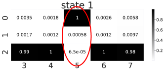
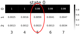
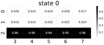
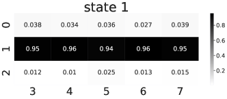
(a)

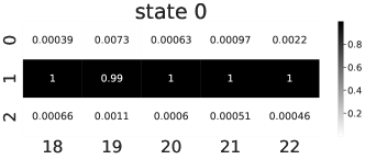
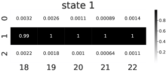
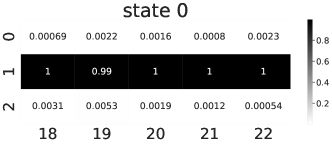
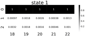
(b)

Figure 2: (a): Visualization of the decoder source (top) and G-RepTransfer (bottom). (b): Visualization of the decoder O-RepTransfer (top) and G-RepTransfer (bottom). For each baseline, The $h$-th column in the $i$-th image denotes the averaged decoded states from the 30 observations generated by latent state $z_{i,h}$, for $i\in\{0,1,2\}$ and $h\in[25]$, from the corresponding target environment. The optimal decoder should recover the latent states up to a permutation. In Fig a (top), note that the learned features in source task fail to solve the target because of the collapse at timestep 5: both observations from state 0 and 1 are mapped to state 0. Note in the source task where this feature is trained, such collapse can happen when state $0$ and $1$ have identical latent transition (for detailed discussion we refer to Misra et al. (2020)). In Fig b (top), RepTransfer with only online access learns an incorrect decoder when the source tasks’ observation spaces are disjoint. This is because the learned feature can decode each source task with a different permutation.

J.6.1 Visualizations from the observational coverage experiment

We record the visualization of the 5 sources from Fig. 3 to Fig. 7; O-RepTransfer in Fig.8; G-RepTransfer in Fig. 9; running Briee on target in Fig. 10.

Figure 3: Visualization of decoders from source 1. Note the collapse happens at timestep 5, 9 and 17.

Figure 4: Visualization of decoders from source 2. Note the collapse happens at timestep 1 and 10.

Figure 5: Visualization of decoders from source 3. Note the collapse happens at timestep 14 and 15.

Figure 6: Visualization of decoders from source 4. Note the collapse happens at timestep 7, 16, 24.

Figure 7: Visualization of decoders from source 3. Note the collapse happens at timestep 13 and 16.

Figure 8: Visualization of decoders from O-RepTransfer

Figure 9: Visualization of decoders from G-RepTransfer

Figure 10: Visualization of decoders from running Briee on target.

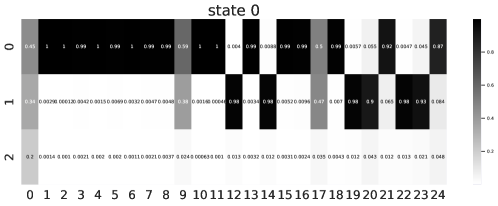
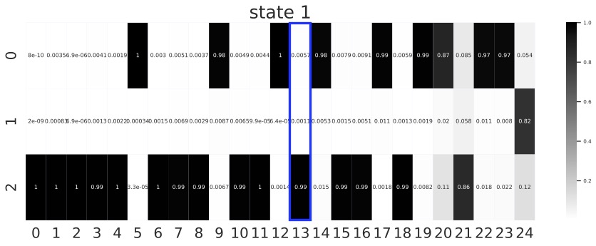
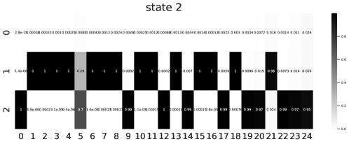
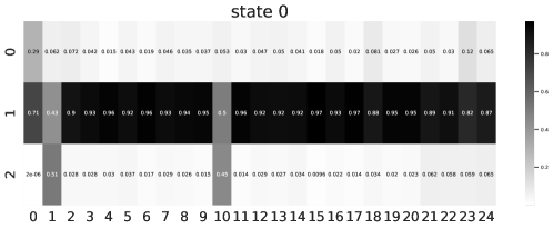
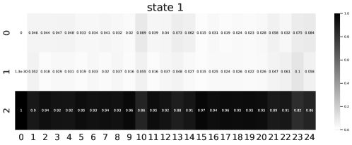
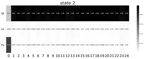
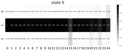
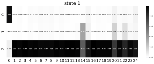
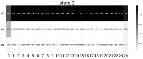
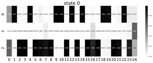
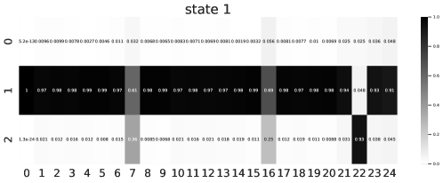
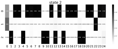
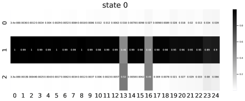
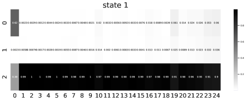
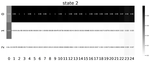
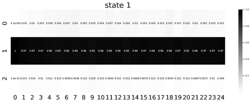
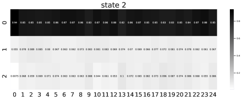
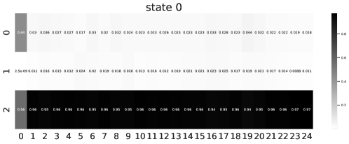
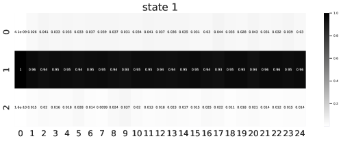
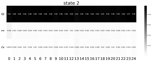
J.6.2 Visualizations from the feature coverage experiment

We record the visualization of the 2 sources from Fig. 11 and Fig. 12; O-RepTransfer in Fig.13; G-RepTransfer in Fig. 14; running Briee on target in Fig. 15. Note that the features collapse at some timesteps in Fig. 14 and Fig. 15, but this is acceptable because the optimal actions at those timesteps are the same for the collapsed states.

Figure 11: Visualization of decoders from source environment 1.

Figure 12: Visualization of decoders from source environment 2.

Figure 13: Visualization of decoders from O-RepTransfer.

Figure 14: Visualization of decoders from G-RepTransfer.

Figure 15: Visualization of decoders running Briee in the target.

References

- Agarwal et al. (2019) Alekh Agarwal, Nan Jiang, Sham M Kakade, and Wen Sun. Reinforcement learning: Theory and algorithms. CS Dept., UW Seattle, Seattle, WA, USA, Tech. Rep, 2019.
- Agarwal et al. (2020) Alekh Agarwal, Sham Kakade, Akshay Krishnamurthy, and Wen Sun. Flambe: Structural complexity and representation learning of low rank mdps. In Advances in Neural Information Processing Systems, volume 33, pages 20095–20107, 2020.
- Arora et al. (2020) Sanjeev Arora, Simon Du, Sham Kakade, Yuping Luo, and Nikunj Saunshi. Provable representation learning for imitation learning via bi-level optimization. In International Conference on Machine Learning, pages 367–376. PMLR, 2020.
- Ayoub et al. (2020) Alex Ayoub, Zeyu Jia, Csaba Szepesvari, Mengdi Wang, and Lin Yang. Model-based reinforcement learning with value-targeted regression. In International Conference on Machine Learning, pages 463–474. PMLR, 2020.
- Barreto et al. (2017) André Barreto, Will Dabney, Rémi Munos, Jonathan J Hunt, Tom Schaul, Hado P van Hasselt, and David Silver. Successor features for transfer in reinforcement learning. Advances in neural information processing systems, 30, 2017.
- Bengio et al. (2009) Yoshua Bengio, Jérôme Louradour, Ronan Collobert, and Jason Weston. Curriculum learning. In Proceedings of the 26th annual international conference on machine learning, pages 41–48, 2009.
- Blier et al. (2021) Léonard Blier, Corentin Tallec, and Yann Ollivier. Learning successor states and goal-dependent values: A mathematical viewpoint. arXiv preprint arXiv:2101.07123, 2021.
- Brunskill and Li (2013) Emma Brunskill and Lihong Li. Sample complexity of multi-task reinforcement learning. arXiv preprint arXiv:1309.6821, 2013.
- Brunskill and Li (2014) Emma Brunskill and Lihong Li. Pac-inspired option discovery in lifelong reinforcement learning. In International conference on machine learning, pages 316–324. PMLR, 2014.
- Caruana (1997) Rich Caruana. Multitask learning. Machine learning, 28(1):41–75, 1997.
- Cheng et al. (2022) Yuan Cheng, Songtao Feng, Jing Yang, Hong Zhang, and Yingbin Liang. Provable benefit of multitask representation learning in reinforcement learning. arXiv preprint arXiv:2206.05900, 2022.
- Cutkosky et al. (2021) Ashok Cutkosky, Christoph Dann, Abhimanyu Das, Claudio Gentile, Aldo Pacchiano, and Manish Purohit. Dynamic balancing for model selection in bandits and rl. In International Conference on Machine Learning, pages 2276–2285. PMLR, 2021.
- Dayan (1993) Peter Dayan. Improving generalization for temporal difference learning: The successor representation. Neural computation, 5(4):613–624, 1993.
- D’Eramo et al. (2019) Carlo D’Eramo, Davide Tateo, Andrea Bonarini, Marcello Restelli, and Jan Peters. Sharing knowledge in multi-task deep reinforcement learning. In International Conference on Learning Representations, 2019.
- Du et al. (2019) Simon Du, Akshay Krishnamurthy, Nan Jiang, Alekh Agarwal, Miroslav Dudik, and John Langford. Provably efficient rl with rich observations via latent state decoding. In International Conference on Machine Learning, pages 1665–1674. PMLR, 2019.
- Du et al. (2020) Simon S Du, Wei Hu, Sham M Kakade, Jason D Lee, and Qi Lei. Few-shot learning via learning the representation, provably. arXiv preprint arXiv:2002.09434, 2020.
- Du et al. (2021) Simon S Du, Sham M Kakade, Jason D Lee, Shachar Lovett, Gaurav Mahajan, Wen Sun, and Ruosong Wang. Bilinear classes: A structural framework for provable generalization in rl. International Conference on Machine Learning, 2021.
- Farahmand and Szepesvári (2011) Amir-massoud Farahmand and Csaba Szepesvári. Model selection in reinforcement learning. Machine learning, 85(3):299–332, 2011.
- Finn et al. (2017) Chelsea Finn, Pieter Abbeel, and Sergey Levine. Model-agnostic meta-learning for fast adaptation of deep networks. In International conference on machine learning, pages 1126–1135. PMLR, 2017.
- Hao et al. (2021a) Botao Hao, Yaqi Duan, Tor Lattimore, Csaba Szepesvári, and Mengdi Wang. Sparse feature selection makes batch reinforcement learning more sample efficient. In International Conference on Machine Learning, pages 4063–4073. PMLR, 2021a.
- Hao et al. (2021b) Botao Hao, Tor Lattimore, Csaba Szepesvári, and Mengdi Wang. Online sparse reinforcement learning. In International Conference on Artificial Intelligence and Statistics, pages 316–324. PMLR, 2021b.
- Hu et al. (2021) Jiachen Hu, Xiaoyu Chen, Chi Jin, Lihong Li, and Liwei Wang. Near-optimal representation learning for linear bandits and linear rl. In International Conference on Machine Learning, pages 4349–4358. PMLR, 2021.
- Huang et al. (2023) Baihe Huang, Jason D. Lee, Zhaoran Wang, and Zhuoran Yang. Provably efficient multi-task reinforcement learning in large state spaces, 2023. URL https://openreview.net/forum?id=p6wiThIOS5m.
- Jiang et al. (2015) Nan Jiang, Alex Kulesza, and Satinder Singh. Abstraction selection in model-based reinforcement learning. In International Conference on Machine Learning, pages 179–188. PMLR, 2015.
- Jiang et al. (2017) Nan Jiang, Akshay Krishnamurthy, Alekh Agarwal, John Langford, and Robert E Schapire. Contextual decision processes with low bellman rank are pac-learnable. In International Conference on Machine Learning, pages 1704–1713. PMLR, 2017.
- Jin et al. (2020a) Chi Jin, Akshay Krishnamurthy, Max Simchowitz, and Tiancheng Yu. Reward-free exploration for reinforcement learning. In International Conference on Machine Learning, pages 4870–4879. PMLR, 2020a.
- Jin et al. (2020b) Chi Jin, Zhuoran Yang, Zhaoran Wang, and Michael I Jordan. Provably efficient reinforcement learning with linear function approximation. In Conference on Learning Theory, pages 2137–2143. PMLR, 2020b.
- Lazaric et al. (2013) Alessandro Lazaric, Emma Brunskill, et al. Sequential transfer in multi-armed bandit with finite set of models. Advances in Neural Information Processing Systems, 26, 2013.
- Lecarpentier et al. (2021) Erwan Lecarpentier, David Abel, Kavosh Asadi, Yuu Jinnai, Emmanuel Rachelson, and Michael L Littman. Lipschitz lifelong reinforcement learning. In Proceedings of the AAAI Conference on Artificial Intelligence, volume 35, pages 8270–8278, 2021.
- Lee et al. (2021) Jonathan Lee, Aldo Pacchiano, Vidya Muthukumar, Weihao Kong, and Emma Brunskill. Online model selection for reinforcement learning with function approximation. In International Conference on Artificial Intelligence and Statistics, pages 3340–3348. PMLR, 2021.
- Lu et al. (2021) Rui Lu, Gao Huang, and Simon S Du. On the power of multitask representation learning in linear mdp. arXiv preprint arXiv:2106.08053, 2021.
- Lykouris et al. (2021) Thodoris Lykouris, Max Simchowitz, Alex Slivkins, and Wen Sun. Corruption-robust exploration in episodic reinforcement learning. In Conference on Learning Theory, pages 3242–3245. PMLR, 2021.
- Maurer et al. (2016) Andreas Maurer, Massimiliano Pontil, and Bernardino Romera-Paredes. The benefit of multitask representation learning. Journal of Machine Learning Research, 17(81):1–32, 2016.
- Misra et al. (2019) Dipendra Misra, Mikael Henaff, Akshay Krishnamurthy, and John Langford. Kinematic state abstraction and provably efficient rich-observation reinforcement learning. arXiv preprint arXiv:1911.05815, 2019.
- Misra et al. (2020) Dipendra Misra, Mikael Henaff, Akshay Krishnamurthy, and John Langford. Kinematic state abstraction and provably efficient rich-observation reinforcement learning. In International conference on machine learning, pages 6961–6971. PMLR, 2020.
- Modi et al. (2020) Aditya Modi, Nan Jiang, Ambuj Tewari, and Satinder Singh. Sample complexity of reinforcement learning using linearly combined model ensembles. In International Conference on Artificial Intelligence and Statistics, pages 2010–2020. PMLR, 2020.
- Modi et al. (2021) Aditya Modi, Jinglin Chen, Akshay Krishnamurthy, Nan Jiang, and Alekh Agarwal. Model-free representation learning and exploration in low-rank mdps. arXiv preprint arXiv:2102.07035, 2021.
- Pacchiano et al. (2020) Aldo Pacchiano, Christoph Dann, Claudio Gentile, and Peter Bartlett. Regret bound balancing and elimination for model selection in bandits and rl. arXiv preprint arXiv:2012.13045, 2020.
- Pan and Yang (2009) Sinno Jialin Pan and Qiang Yang. A survey on transfer learning. IEEE Transactions on knowledge and data engineering, 22(10):1345–1359, 2009.
- Parisi et al. (2019) German I Parisi, Ronald Kemker, Jose L Part, Christopher Kanan, and Stefan Wermter. Continual lifelong learning with neural networks: A review. Neural Networks, 113:54–71, 2019.
- Parisotto et al. (2015) Emilio Parisotto, Jimmy Lei Ba, and Ruslan Salakhutdinov. Actor-mimic: Deep multitask and transfer reinforcement learning. arXiv preprint arXiv:1511.06342, 2015.
- Ren et al. (2021) Tongzheng Ren, Tianjun Zhang, Csaba Szepesvári, and Bo Dai. A free lunch from the noise: Provable and practical exploration for representation learning. arXiv preprint arXiv:2111.11485, 2021.
- Rusu et al. (2016) Andrei A Rusu, Neil C Rabinowitz, Guillaume Desjardins, Hubert Soyer, James Kirkpatrick, Koray Kavukcuoglu, Razvan Pascanu, and Raia Hadsell. Progressive neural networks. arXiv preprint arXiv:1606.04671, 2016.
- Touati and Ollivier (2021) Ahmed Touati and Yann Ollivier. Learning one representation to optimize all rewards. Advances in Neural Information Processing Systems, 34:13–23, 2021.
- Tripuraneni et al. (2020) Nilesh Tripuraneni, Michael Jordan, and Chi Jin. On the theory of transfer learning: The importance of task diversity. Advances in Neural Information Processing Systems, 33:7852–7862, 2020.
- Uehara et al. (2021) Masatoshi Uehara, Xuezhou Zhang, and Wen Sun. Representation learning for online and offline rl in low-rank mdps. In International Conference on Learning Representations, 2021.
- Wagenmaker et al. (2022) Andrew Wagenmaker, Yifang Chen, Max Simchowitz, Simon S Du, and Kevin Jamieson. Reward-free rl is no harder than reward-aware rl in linear markov decision processes. arXiv preprint arXiv:2201.11206, 2022.
- Wang et al. (2020) Ruosong Wang, Simon S Du, Lin Yang, and Russ R Salakhutdinov. On reward-free reinforcement learning with linear function approximation. Advances in neural information processing systems, 33:17816–17826, 2020.
- Yang et al. (2020) Jiaqi Yang, Wei Hu, Jason D Lee, and Simon Shaolei Du. Impact of representation learning in linear bandits. In International Conference on Learning Representations, 2020.
- Yang et al. (2022) Jiaqi Yang, Qi Lei, Jason D Lee, and Simon S Du. Nearly minimax algorithms for linear bandits with shared representation. arXiv preprint arXiv:2203.15664, 2022.
- Zanette et al. (2021) Andrea Zanette, Ching-An Cheng, and Alekh Agarwal. Cautiously optimistic policy optimization and exploration with linear function approximation. COLT, 2021.
- Zhang et al. (2021) Weitong Zhang, Jiafan He, Dongruo Zhou, Amy Zhang, and Quanquan Gu. Provably efficient representation learning in low-rank markov decision processes. arXiv preprint arXiv:2106.11935, 2021.
- Zhang et al. (2020) Xuezhou Zhang, Yuzhe Ma, and Adish Singla. Task-agnostic exploration in reinforcement learning. Advances in Neural Information Processing Systems, 33:11734–11743, 2020.
- Zhang et al. (2022) Xuezhou Zhang, Yuda Song, Masatoshi Uehara, Mengdi Wang, Wen Sun, and Alekh Agarwal. Efficient reinforcement learning in block mdps: A model-free representation learning approach. arXiv preprint arXiv:2202.00063, 2022.
- Zhu et al. (2020) Zhuangdi Zhu, Kaixiang Lin, and Jiayu Zhou. Transfer learning in deep reinforcement learning: A survey. arXiv preprint arXiv:2009.07888, 2020.