Conditionally Calibrated Predictive Distributions by Probability-Probability Map: Application to Galaxy Redshift Estimation and Probabilistic Forecasting

Abstract

Uncertainty quantification is crucial for assessing the predictive ability of AI algorithms. Much research has been devoted to describing the predictive distribution (PD) $F(y|{\mathbf{x}})$ of a target variable $y\in\mathbb{R}$ given complex input features ${\mathbf{x}}\in\mathcal{X}$. However, off-the-shelf PDs (from, e.g., normalizing flows and Bayesian neural networks) often lack conditional calibration with the probability of occurrence of an event given input ${\mathbf{x}}$ being significantly different from the predicted probability. Current calibration methods do not fully assess and enforce conditionally calibrated PDs. Here we propose Cal-PIT, a method that addresses both PD diagnostics and recalibration by learning a single probability-probability map from calibration data. The key idea is to regress probability integral transform scores against ${\mathbf{x}}$. The estimated regression provides interpretable diagnostics of conditional coverage across the feature space. The same regression function morphs the misspecified PD to a re-calibrated PD for all ${\mathbf{x}}$. We benchmark our corrected prediction bands (a by-product of corrected PDs) against oracle bands and state-of-the-art predictive inference algorithms for synthetic data. We also provide results for two applications: (i) conditional density estimation of galaxy distances given imaging data (so-called photometric redshift estimation), and (ii) probabilistic nowcasting given sequences of satellite images.

, , ,
, , and

1 Introduction

Prediction bands are useful in quantifying uncertainties in predictive algorithms, but we have over the past couple of decades witnessed a transformation across scientific disciplines from point forecasts to the entire predictive distribution (PD) of a (continuous) response or “target” variable $Y$ given input features or covariates $X$; see, e.g., Gneiting (2008) for probabilistic forecasting in weather predictions, Timmermann (2000) for financial risk management, Alkema, Raftery and Clark (2007) for epidemiological projections, and Mandelbaum et al. (2008) and Malz and Hogg (2022) for the importance of PDs for astrophysical studies. There are broadly speaking two main forces behind this paradigm shift. First, new survey technology in the engineering, physical and biological sciences is producing data of unprecedented depth, richness and scope. To fully leverage these data in down-stream analysis, we need more precise estimates of the uncertainty in predicted quantities in terms of predictive (or posterior) distributions. Second, we are experiencing a rapid growth of high-capacity machine learning algorithms that allow such quantification for complex data of different modalities, including, e.g., sequences of satellite images combined with other observational data.

Approaches to obtaining PDs can roughly be divided into the following categories:

• conditional density estimation (CDE), which directly estimates the conditional density functions $f(y|{\mathbf{x}})$ via, e.g., mixture density networks (MDN; Bishop 1994), kernel mixture networks (Ambrogioni et al., 2017), Bayesian neural networks (see e.g. Goan and Fookes 2020 and references therein), normalizing flows including neural autoregressive models (Papamakarios et al., 2019a; Kobyzev, Prince and Brubaker, 2021), Gaussian process CDEs (Dutordoir et al., 2018), or simpler nonparametric CDE methods (Izbicki and Lee, 2016; Izbicki and Lee, 2017; Dalmasso et al., 2020a);

• implicit CDE methods, which encode the PD implicitly, e.g., variational autoencoders (VAEs; Kingma and Welling 2013), conditional generative adversarial networks (cGANs; Mirza and Osindero 2014), diffusion models (Sohl-Dickstein et al., 2015; Ho, Jain and Abbeel, 2020; Nichol and Dhariwal, 2021; Dhariwal and Nichol, 2021; Ho and Salimans, 2022) and transformer-based generative models (Vaswani et al., 2017; Radford et al., 2019);

• quantile regression methods that estimate all quantiles simultaneously (Chung et al., 2021a; Fasiolo et al., 2021; Tagasovska and Lopez-Paz, 2019; Amerise, 2018; Liu and Wu, 2011).

• dropout and other ensemble techniques, which estimate the uncertainty about $y$ by generating multiple predictions using different models (Gal and Ghahramani, 2016; Lakshminarayanan, Pritzel and Blundell, 2017; Rahaman et al., 2021).

1.1 Conditional versus Marginal Calibration

Though there are many ways one can quantify uncertainties in a regression setting, PDs can lead to overly optimistic or misleading conclusions regarding a model’s predictive ability unless the PD approximately satisfies individual or conditional calibration, meaning that the estimated predicted distribution $\widehat{F}(y|{\mathbf{x}})=F(y|{\mathbf{x}})$ for all $y\in\mathbb{R}$ and all ${\mathbf{x}}\in\mathcal{X}$. In words, the predicted conditional probability of an event happening given input ${\mathbf{x}}$ should match its observed probability, regardless of the value of ${\mathbf{x}}$. Such instance-wise uncertainties are crucial in practical applications. For example, for weather forecasts that predict the probability of rainfall given the current state of environmental predictors, and for medical research that estimate the efficacy of a drug for individuals of specific demographics after taking a given dose. Achieving instance-wise uncertainties can also be important for algorithmic fairness so as not to over- or under-predict risks for certain groups of individuals (Kleinberg, Mullainathan and Raghavan, 2016; Zhao, Ma and Ermon, 2020).

Individual calibration can however be difficult to verify. Most works instead consider a weaker notion of calibration such as average or marginal calibration,

$${\mathbb{E}}_{{\mathbf{X}}\sim F_{{\mathbf{X}}}}\left[{\mathbb{E}}_{Y\sim F_{Y|{\mathbf{X}}}}\left[{\mathbb{I}}\left(\widehat{F}(Y|{\mathbf{X}})\leq p\right)\right]\right]=p,\ \ \forall p\in[0,1].$$

Indeed, average calibration is often simply referred to as just “calibration” (see, e.g., Gneiting and Katzfuss 2014; Kuleshov, Fenner and Ermon 2018).

1.2 Predictive Distributions and Prediction Sets

From PDs, one can derive various quantities of interest, such as moments, kurtosis, prediction intervals, or even more general prediction bands; such as Highest Predictive Density (HPD) regions. By construction, individually calibrated PDs lead to conditionally valid prediction bands: if $C_{\alpha}({\mathbf{X}})$ is a prediction band derived from $\widehat{F}$ with nominal coverage $1-\alpha$, individually calibrated prediction distributions $\widehat{F}$ imply

$$\mathbb{P}(Y\in C_{\alpha}({\mathbf{X}})|{\mathbf{X}}={\mathbf{x}})=1-\alpha,\ \ \forall{\mathbf{x}}\in\mathcal{X}.$$ (1)

On the other hand, it is difficult to convert prediction sets and quantile estimates to entire PDs without additional assumptions. That is, calibrated PDs implies calibrated prediction sets but not vice versa.

1.3 Motivating Applications

Our work is motivated by two main applications in the physical sciences:

(i) Estimating photometric redshifts of galaxies. Redshift ($z$) is a measurable proxy for the distance to a galaxy and is crucial for studies of astrophysics and cosmology. Direct redshift measurement via spectroscopy is however not feasible for a very large number of galaxies. Redshift estimates are hence often predicted from less resource-intensive imaging data, resulting in measurements called photometric redshifts or photo-$z$’s.

Upcoming multi-billion dollar cosmology experiments like the Rubin Observatory’s Legacy Survey of Space and Time (LSST) will crucially depend on photo-$z$’s to achieve its science goals. Moreover, for cosmological applications, prediction intervals are not sufficient and full distributions are required due to the presence of multi-modality within such distributions. The requirements for the precision of photo-$z$ CDEs are extremely stringent: errors in the moments of the distributions should be within $\sim 0.1\%$ of the truth for any downstream physical analysis to not be affected (The LSST Dark Energy Science Collaboration et al., 2018). We have chosen the photo-$z$ application because of its high impact on the physical sciences, and because of clear existing benchmarks against state-of-the-art photo-$z$ estimation methods made available via the LSST-Dark Energy Science Collaboration photo-$z$ data challenge (Schmidt et al., 2020).

(ii) Probabilistic Forecasting of Tropical Cyclone Intensity from Satellite Imagery. Tropical cyclones are highly organized, rotating storms that are among the most costly natural disasters in the United States. TC intensity forecasts have improved in recent years, but these improvements have been relatively slow during the last decade compared to improvements in track forecasts, particularly at 24-hour lead times (DeMaria et al., 2014). The latest generation of geostationary satellites (GOES), such as GOES-16, now provides unprecedented spatio-temporal resolution of TC structure and evolution (Schmit et al., 2017). A broad array of recent works involving neural networks has explored the wealth of information of GOES imagery for TC short-term intensity prediction (e.g., Olander et al. 2021; Griffin, Wimmers and Velden 2022), but so far statistical forecasting techniques have not been able to produce ensemble or probabilistic forecasts that reliably quantify uncertainty in the predictions.

1.4 Challenges: Miscalibration and Lack of Diagnostics for Conditional Coverage

Off-the-shelf PDs, such as the ones listed above, are usually far from being even marginally calibrated: CDEs and quantile regression methods are typically fitted by minimizing a loss function that does not directly depend upon calibration. Examples of such loss functions include, e.g, the KL divergence, integral probability metrics (Papamakarios et al., 2019b; Dalmasso et al., 2020b), and the pinball loss (Koenker and Hallock, 2001). As noted by, e.g., Guo et al. (2017) and Chung et al. (2021b, Proposition 1), modern machine learning methods tend to unequally favor prediction accuracy and sharpness calibration. Different solutions have been proposed, including proposing new loss functions that trade off sharpness and calibration (Chung et al., 2021b), and loss functions that enforce independence of sharpness and coverage (Feldman, Bates and Romano, 2021).

An additional obstacle to achieving conditional calibration (beyond constructing loss functions that enforce instance-wise uncertainty quantification) is that most metrics that assess the calibration of PDs — such as the widely adopted probability integral transform (PIT; Gan and Koehler 1990) and simulator-based calibration (SBC; Talts et al. 2018) — only assess average or marginal calibration over the entire distribution of ${\mathbf{X}}\in\mathcal{X}$. As noted by, e.g., Schmidt et al. (2020), the PIT statistic may be uniformly distributed even if $\widehat{F}(y|{\mathbf{x}})=F(y)$; that is, when the CDE completely ignores the input ${\mathbf{x}}$. More generally, inconsistencies in various regions of the feature space can cancel out to produce optimal results when looked at as an ensemble (Zhao et al., 2021; Jitkrittum, Kanagawa and Schölkopf, 2020a; Luo et al., 2021).

To ensure reliable uncertainty quantification of predictive models, there is both a need for (i) methods that can produce PDs that are approximately calibrated for all ${\mathbf{x}}$, and for (ii) interpretable and computationally tractable diagnostics that can assess calibration across the entire feature space.

1.5 Our Approach

We propose a two-pronged non-parametric approach of diagnostics of conditional densities with a means of visualization, followed by recalibration which reliably quantifies individual uncertainties (thereby providing local consistency, Definition 2).

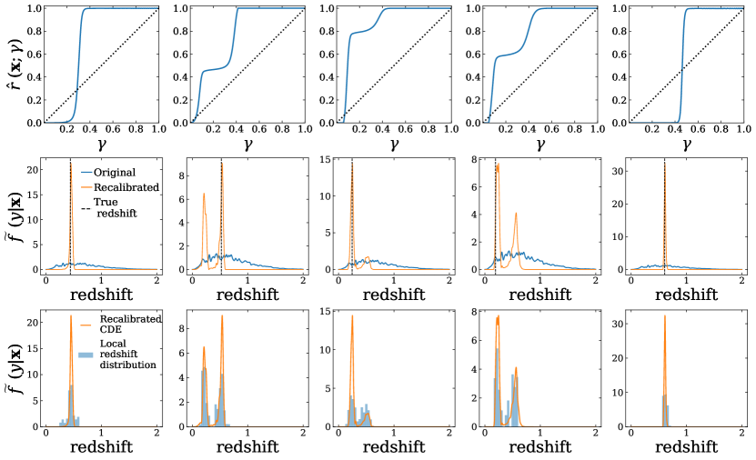
Our approach builds on the key observation that an estimate $\widehat{F}$ is locally consistent if and only if its probability integral transform (PIT) value ${\rm PIT}(Y;{\mathbf{X}}):=\widehat{F}(Y|{\mathbf{X}})$ is uniformly distributed conditionally on ${\mathbf{x}}$. Thus, if a model is well-calibrated, $r^{\widehat{f}}(\gamma;{\mathbf{x}}):=\mathbb{P}\left({\rm PIT}(Y;{\mathbf{X}})\leq\gamma\ \middle|\ {\mathbf{x}}\right)$ is close to $\gamma$ for all ${\mathbf{x}}$’s. We achieve this by learning the function $r$ via, for example, monotonic neural networks. Since ${\rm PIT}(y;{\mathbf{x}})<\gamma\iff y\in(-\infty,\widehat{F}^{-1}(\gamma|{\mathbf{x}}))$, the $L^{2}$ loss function used for training directly targets conditional calibration. Moreover, our procedure is amortized, in the sense that we can train on ${\mathbf{x}}$ and $\gamma$ jointly, after which the function $r$ can be evaluated for any ${\mathbf{x}}$’s and $\gamma$. By evaluating how far $r^{\widehat{f}}(\gamma;{\mathbf{x}})$ is from $\gamma$, one can assess at what locations in feature space $\widehat{F}$ is well-estimated. Of particular note is that the learnt function $\widehat{r}^{\widehat{f}}(\gamma;{\mathbf{x}})$ itself suggests how $\widehat{F}$ should be adjusted. We are providing the practitioner with interpretable quantification and visualization tools of potential modes of failures across the entire feature space via so-called Amortized Local P-P plots (see Figure 2), together with a means to correcting such discrepancies via a P-P map (Equation 6). Figure 8 showcases the valuable insights Cal-PIT offers for our main photo-z application. The top row provides information concerning the deviations between estimated and true redshift distributions. The center row shows recalibrated estimates. By reshaping the original densities via the P-P map, our method is able to recover multimodal distributions, as illustrated by the bottom row.

1.6 Relation to Other Methods

Goodness-of-Fit Tests and Calibration

Goodness-of-fit of conditional density models to observed data can be assessed by two-sample tests (Stute and Zhu, 2002; Moreira, 2003; Jitkrittum, Kanagawa and Schölkopf, 2020b). Such tests are useful for deciding whether a PD needs to be improved, but do not provide any means to correct discrepancies.

One way to recalibrate PDs (proposed by, e.g., Bordoloi, Lilly and Amara 2010) is by first assessing how the marginal distribution of the PIT values differs from a uniform distribution by diagnostics tools (Cook, Gelman and Rubin, 2006; Freeman, Izbicki and Lee, 2017; Talts et al., 2018; D’Isanto and Polsterer, 2018), and then applying corrections to bring them into agreement. However, by construction, such recalibration schemes only improve marginal calibration. In this work, we instead build on Zhao et al. (2021), which proposes a version of PIT that is estimated across the entire input feature space, thereby allowing us to directly assess and target conditional coverage.

Quantile Regression

Quantile regression intervals converge to the oracle $C^{*}_{\alpha}({\mathbf{X}})=\left[F^{-1}(0.5\alpha|{\mathbf{X}}),F^{-1}(1-0.5\alpha|{\mathbf{X}})\right]$ (Koenker and Bassett Jr., 1978; Taylor and Bunn, 1999). Even though $C^{*}_{\alpha}({\mathbf{X}})$ satisfies Equation 1, the standard pinball loss can yield highly miscalibrated UQ models for finite data sets (Chung et al., 2021b; Feldman, Bates and Romano, 2021). New loss functions have been proposed to address this issue (Chung et al., 2021b; Feldman, Bates and Romano, 2021). Our approach also provides calibrated prediction regions but is more general — yielding full PDs, and not only prediction intervals.

Conformal Inference

Conformal prediction methods have the appealing property of yielding prediction sets with finite-sample marginal validity, $\mathbb{P}(Y\in C({\mathbf{X}}))\geq 1-\alpha$, as long as the data are exchangeable (Vovk, Gammerman and Shafer, 2005; Lei et al., 2018). However, there is no guarantee that Equation 1 is satisfied, even approximately. More recent efforts have addressed approximate conditional validity (Romano, Patterson and Candès, 2019; Izbicki, Shimizu and Stern, 2020; Chernozhukov, Wüthrich and Zhu, 2021; Izbicki, Shimizu and Stern, 2022) by designing conformal scores with an approximately homogeneous distribution across $\mathcal{X}$. Unfortunately, it is difficult to check whether these methods provide good conditional coverage in practice. Conformal prediction bands are also not conditionally valid, even asymptotically, if the initial model is misspecified. Finally, unlike conformal inference, our method provides estimates of the full PD.

Optimal Transport

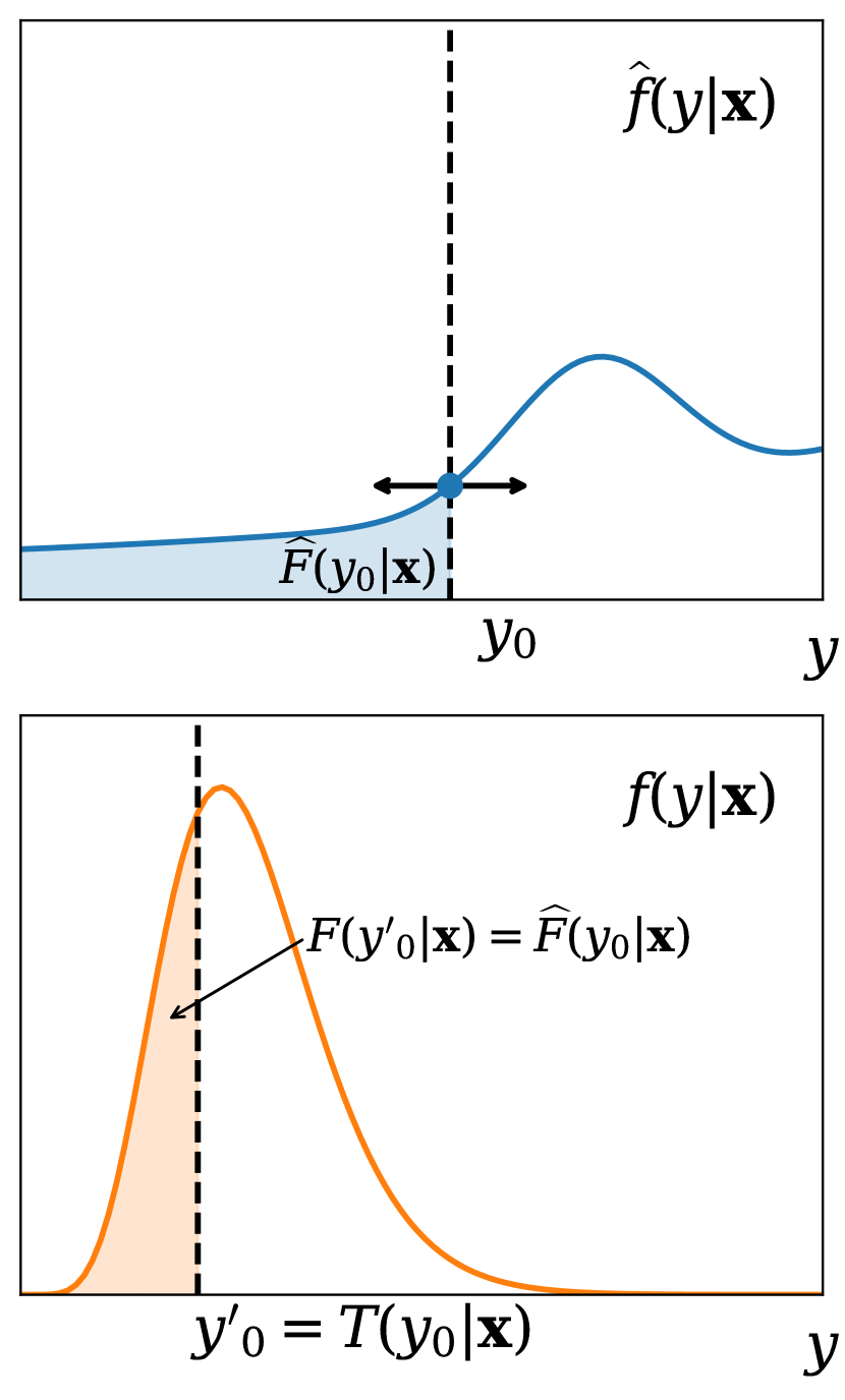
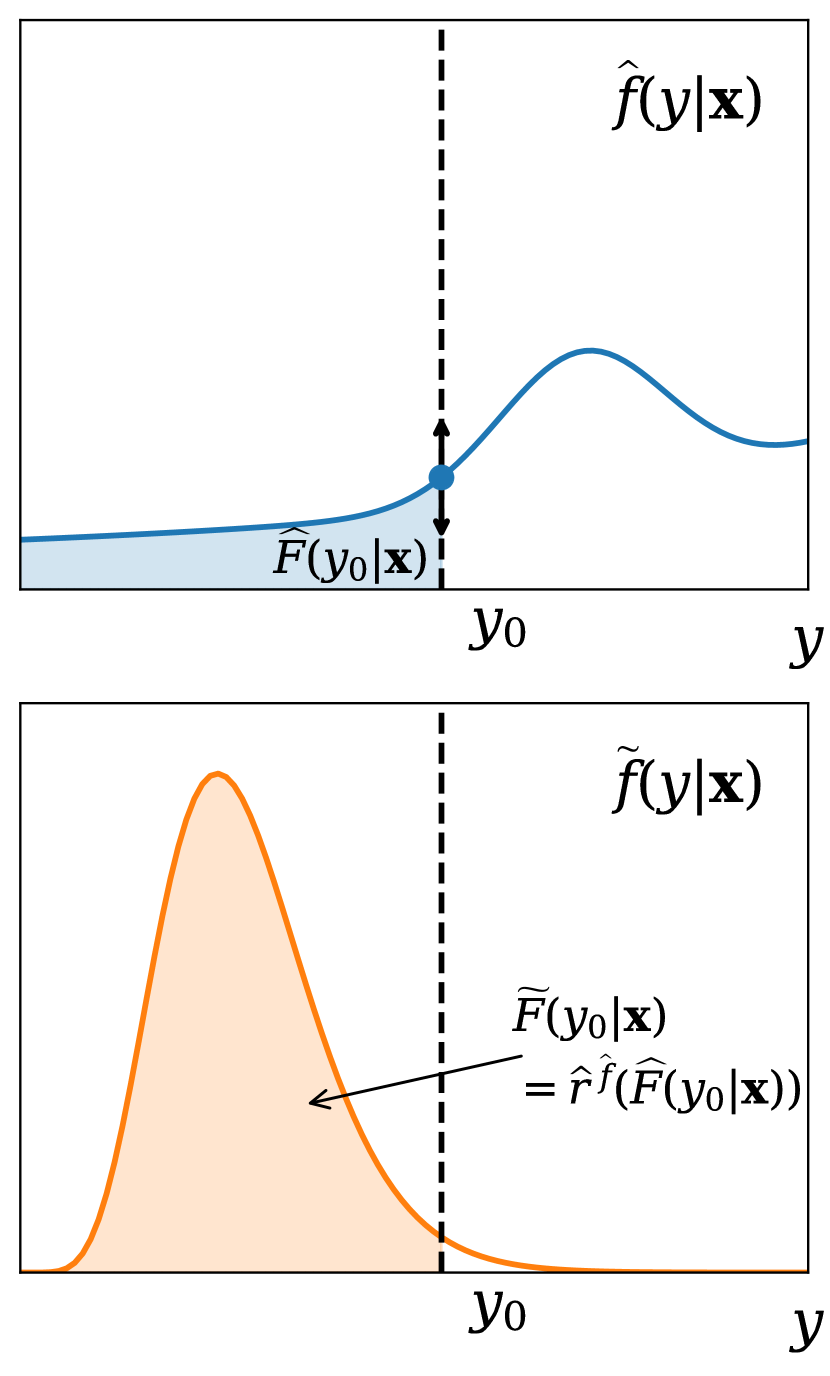
Cal-PIT can be thought of as a regression approach to estimating the optimal transport (see Appendix A for a review of optimal transport) that morphs a reference distribution $\widehat{F}(y|{\mathbf{x}})$ into a target distribution $F(y|{\mathbf{x}})$. Figure 1 illustrates the parallel views of Cal-PIT and Optimal Transport (OT). The details are as follows:

Let $Y\sim\widehat{F}_{Y|{\mathbf{X}}}$ and $Y^{\prime}\sim F_{Y|{\mathbf{X}}}$ be continuous random variables with respective conditional densities $\widehat{f}(y|{\mathbf{x}})$ and $f(y|{\mathbf{x}})$. We assume that $Y,Y^{\prime}\in\mathcal{Y}\subseteq\mathbb{R}$ and ${\mathbf{X}}\in\mathcal{X}\subseteq\mathbb{R}^{d}$, where $d$ can be large. We also assume that we have access to an i.i.d. sample or “calibration set” $\mathcal{D}=\{({\mathbf{X}}^{\prime}_{1},Y^{\prime}_{1}),...,({\mathbf{X}}^{\prime}_{n},Y^{\prime}_{n})\}$ from the joint distribution $F_{{\mathbf{X}},Y}$ of the target data ${\mathbf{X}}$ and $Y$.

For every fixed ${\mathbf{x}}\in\mathcal{X}$, there exists a unique optimal transport map $T_{{\mathbf{x}}}:\mathcal{Y}\rightarrow\mathcal{Y}$ for all strictly convex functions, such that the distribution of $T_{{\mathbf{x}}}(Y):=T(Y|{\mathbf{x}})$ is $F_{Y|{\mathbf{x}}}$ (Santambrogio, 2015).

The OT solution performs quantile matching so that $F(y^{\prime}_{0}|{\mathbf{x}})=\widehat{F}(y_{0}|{\mathbf{x}}),$ for every $y_{0}\in\mathcal{Y}$ (as illustrated in the left panel of Figure 1), where the OT map is given by

$$T(y_{0}|{\mathbf{x}}):=F^{-1}\left(\widehat{F}(y_{0}|{\mathbf{x}})|{\mathbf{x}}\right).$$ (2)

However, it is difficult to perform conditional quantile matching in practice, as the CDF $F(\cdot|{\mathbf{x}})$ is unknown and difficult to estimate well across the feature space $\mathcal{X}$ for high-dimensional covariates ${\mathbf{x}}$. In fact, that was the original motivation for this work.

Instead of conditional quantile matching, the Cal-PIT approach morphs the density $\widehat{f}(y|{\mathbf{x}})$ into a new density $\widetilde{f}(y|{\mathbf{x}})$ by mapping probabilities (as illustrated in the right panel of Figure 1) through $\widetilde{F}\left(y_{0}|{\mathbf{x}}\right):=\widehat{r}^{\widehat{f}}\left(\widehat{F}(y_{0}|{\mathbf{x}});{\mathbf{x}}\right),$ for every $y_{0}\in\mathcal{Y}$ and ${\mathbf{x}}\in\mathcal{X}$. The value of this approach is that $\widehat{F}(\cdot|{\mathbf{x}})$ is known, and we can directly compute the conditional P-P map $\widehat{r}^{\widehat{f}}(\gamma;{\mathbf{x}})$ by regressing a scalar quantity against ${\mathbf{x}}$ and $\gamma$ (Algorithm 1). If we have $\widehat{r}^{\widehat{f}}$, we can also easily derive an estimate of the OT solution (Eq. 2) for every ${\mathbf{x}}\in\mathcal{X}$ by $\widehat{T}(y_{0}|{\mathbf{x}}):=\widetilde{F}^{-1}\left(\widehat{F}(y_{0}|{\mathbf{x}})|{\mathbf{x}}\right).$

(a) OT by Matching Quantiles

(b) Cal-PIT by Mapping Probabilities

Figure 1: Left: The optimal transport (OT) map from $\widehat{F}(y|{\mathbf{x}})$ to $F(y|{\mathbf{x}})$ performs quantile matching for fixed ${\mathbf{x}}$ to match calibration data, where the OT map is given by $T(y_{0}|{\mathbf{x}}):=F^{-1}\left(\widehat{F}(y_{0}|{\mathbf{x}})\mid{\mathbf{x}}\right)$. The OT map rearranges one PDF into another. Right: Cal-PIT constructs an estimate of the entire conditional distribution $F(y|{\mathbf{x}})$ by mapping probabilities, yielding the recalibrated distribution $\widetilde{F}\left(y_{0}|{\mathbf{x}}\right):=\widehat{r}^{\widehat{f}}\left(\widehat{F}(y_{0}|{\mathbf{x}});{\mathbf{x}}\right)$, and hence an estimate of the OT map through $\widehat{T}(y_{0}|{\mathbf{x}}):=\widetilde{F}^{-1}\left(\widehat{F}(y_{0}|{\mathbf{x}})\mid{\mathbf{x}}\right)$ for every ${\mathbf{x}}\in\mathcal{X}$ and $y_{0}\in\mathcal{Y}$. That is, the P-P map reshapes the original PDF, but the end result is the same. Thus, Cal-PIT offers a computationally efficient means to estimating the OT map across a potentially high-dimensional feature space $\mathcal{X}$.

1.7 Contribution and Relevance

The contribution of this paper is two-fold: On the methodology side, we present a unified framework for diagnostics and recalibration of entire predictive distributions through a single P-P map learnt from calibration data. Our approach offers a regression-based approach to estimating an optimal transport map from an initial distribution $F_{0}(y|{\mathbf{x}})$ to a target distribution $F(y|{\mathbf{x}})$ across a potentially high-dimensional feature space. Our method directly targets conditional coverage and provides interpretable diagnostics, with well-calibrated prediction sets as a by-product of our PDs. Although estimating entire distributions nonparametrically is difficult, our methods’s performance, in terms of conditional coverage and efficiency (i.e. tight regions), is on par with state-of-the-art predictive inference algorithms for constructing prediction sets; see Section 4.1 for comparisons. Our method can adjust for model misspecifications; see Section  4.2 for an example of diagnostics and recalibration in a setting with distributional shift. A ready-to-use and flexible implementation of Cal-PIT is available at https://github.com/lee-group-cmu/Cal-PIT.

On the applied side, for photo-z applications, the Cal-PIT method represents a great improvement over the state-of-the-art by ensuring that CDEs are well calibrated everywhere in parameter space, not only as a full ensemble. More generally, our framework can be applied to stationary time series and other settings with dependent high-dimensional data; see Section 5.2 for an example with probabilistic nowcasting based on sequences of images.

Remark 1 (Simulation-Based Calibration of Bayesian Posterior Distributions).

In Bayesian inference, the posterior distribution $F(\theta|{\mathbf{x}})$ is fundamental for quantifying uncertainty about the parameter $\theta$ given the data ${\mathbf{x}}$. In many cases, exact computation of the posterior distribution is intractable, and Markov Chain Monte Carlo (MCMC) methods are used to approximate $F(\theta|{\mathbf{x}})$ (Robert, Casella and Casella, 1999). Recent advances in machine learning algorithms and simulations have also led to the development of simulation-based inference (SBI; Cranmer, Brehmer and Louppe 2020) methods that directly estimate the posterior distribution $F(\theta|{\mathbf{x}})$ from simulated data in settings where the likelihood function is not analytically tractable (Beaumont, Zhang and Balding, 2002; Papamakarios and Murray, 2016; Marin et al., 2012; Lueckmann et al., 2017; Sisson, Fan and Beaumont, 2018; Izbicki, Lee and Pospisil, 2019; Greenberg, Nonnenmacher and Macke, 2019).

Cal-PIT can assess the quality of estimated posterior distributions $\widehat{F}(\theta|{\mathbf{x}})$ from MCMC or Bayesian SBI methods, and if needed, adjust $\widehat{F}(\theta|{\mathbf{x}})$ to be consistent with the posterior distribution $F(\theta|{\mathbf{x}})$ that is associated with the assumed prior and likelihood. For implicit models of $\widehat{F}(\theta|{\mathbf{x}})$, such as MCMC, we approximate the PIT values by forward simulating data. Specifically, for a fixed ${\mathbf{x}}\in\mathcal{X}$ and $\theta\in\Theta$, we draw $\theta_{1},\ldots,\theta_{L}\sim\widehat{F}(\cdot|{\mathbf{x}})$ and approximate ${\rm PIT}(\theta;{\mathbf{x}})$ using $L^{-1}\sum_{i=1}^{L}{\mathbb{I}}(\theta_{i}\leq\theta)$.

Unlike simulation-based calibration (SBC) by Talts et al. (2018), Cal-PIT yields conditionally calibrated posteriors that are approximately locally consistent (Definition 2). The Cal-PIT framework is also different from likelihood-free frequentist inference (LF2I; Dalmasso et al. 2021; Masserano et al. 2022), which constructs and runs diagnostics for frequentist confidence sets based on simulations and a Neyman inversion of hypothesis tests.

2 Methodology

Notation and objectives. Suppose that $\widehat{f}(y|{\mathbf{x}})$ is a conditional density estimate (CDE) of a continuous random variable $Y\in\mathcal{Y}\subseteq\mathbb{R}$ given a random vector ${\mathbf{X}}\in\mathcal{X}\subseteq\mathbb{R}^{d}$. Let $\mathcal{D}=\{({\mathbf{X}}_{1},Y_{1}),...,({\mathbf{X}}_{n},Y_{n})\}$ denote an i.i.d. sample from $F_{{\mathbf{X}},Y}$, the joint distribution of $({\mathbf{X}},Y)$. Our goal is to use $\mathcal{D}$ to recalibrate our CDE, so as to achieve correct conditional coverage. We refer to $\mathcal{D}$ as “calibration data”, which are independent from the “train data” used to construct $\widehat{f}(y|{\mathbf{x}})$.

2.1 Local Consistency Analysis and Diagnostics of PDs

Our calibration framework uses diagnostics developed by Zhao et al. (2021) for assessing conditional density models. For fixed ${\mathbf{x}}\in\mathcal{X}$ and $y\in\mathcal{Y}$, the local probability integral transform (PIT) of $y$ at ${\mathbf{x}}$ is given by

$${\rm PIT}(y;{\mathbf{x}}):=\int_{-\infty}^{y}\widehat{f}(y^{\prime}|{\mathbf{x}})dy^{\prime}=\widehat{F}(y|{\mathbf{x}}).$$ (3)

where $\widehat{F}$ is the predictive distribution associated with $\widehat{f}$. The diagnostics require the estimation of the CDF of the PIT values, which we refer to as the PIT-CDF:

Definition 1 (PIT-CDF).

For every ${\mathbf{x}}\in\mathcal{X}$ and $\gamma\in(0,1)$, the CDF of the local PIT is given by

$$r^{\widehat{f}}(\gamma;{\mathbf{x}}):=\mathbb{P}\left({\rm PIT}(Y;{\mathbf{x}})\leq\gamma\ \middle|\ {\mathbf{x}}\right).$$ (4)

We learn $r^{\widehat{f}}(\gamma;{\mathbf{x}})$ using regression. In this paper, we improve upon Zhao et al. (2021) by first augmenting the calibration data ${\mathcal{D}}$ by drawing multiple values $\gamma_{i,1},\ldots,\gamma_{i,K}\sim U(0,1)$ for each data point ($i=1,\ldots,n$), then regressing the random variable

$$W_{i,j}:={\mathbb{I}}({\rm PIT}(Y_{i};{\mathbf{X}}_{i})\leq\gamma_{i,j})$$ (5)

on both ${\mathbf{X}}_{i}$ and $\gamma_{i,j}$ using the augmented calibration sample $\mathcal{D}^{\prime}=\{({\mathbf{X}}_{i},\gamma_{i,j},W_{i,j})\}_{i,j}$, for $i=1,\ldots,n$ and $j=1,\ldots,K$. As $r^{\widehat{f}}(\gamma;{\mathbf{x}})$ is a non-decreasing function of $\gamma$, we use monotonic neural networks (Wehenkel and Louppe, 2019) for most applications with complex inputs, though any other suitable regression method may be used.

The PIT-CDF values $r^{\widehat{f}}(\gamma;{\mathbf{x}})$ characterize the local consistency of $\widehat{f}$, defined as follows:

Definition 2 (Local consistency).

A density estimate $\widehat{f}(\cdot|{\mathbf{x}})$ is locally consistent at a fixed ${\mathbf{x}}$ if, and only if, $\widehat{F}(\cdot|{\mathbf{x}})=F(\cdot|{\mathbf{x}})$.

Indeed, for fixed ${\mathbf{x}}$, $\widehat{f}(\cdot|{\mathbf{x}})$ is locally consistent, if and only if, the distribution of ${\rm PIT}(Y;{\mathbf{x}})$ is uniform over $(0,1)$ (conditionally on ${\mathbf{x}}$), which is also equivalent to $r^{\widehat{f}}(\gamma;{\mathbf{x}})=\gamma$ for every $\gamma\in(0,1)$ (Zhao et al., 2021, Corollary 1).

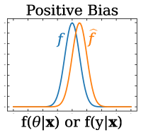
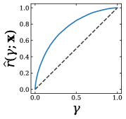
By creating a graphical plot of $r^{\widehat{f}}(\gamma;{\mathbf{x}})$ versus $\gamma$, referred to as an Amortized Local Probability-Probability Plot (ALP), we can assess how close $\widehat{f}$ is to $f$ across the entire feature space. Figure 2 illustrates how these ALPs provide interpretable information regarding possible modes of deviation.

BIAS                                                      DISPERSION

Figure 2: P-P plots are commonly used to assess how well a density model fits actual data. Such plots display, in a clear and interpretable way, effects like bias (left panel) and dispersion (right panel) in an estimated distribution $\widehat{f}$ vis-a-vis the true data-generating distribution $f$. Our framework yields a computationally efficient way to constructing “Amortized Local P-P Plots” (ALPs), for comparing conditional densities $\widehat{f}(\theta|{\mathbf{x}})$ or $\widehat{f}(y|{\mathbf{x}})$ at any location ${\mathbf{x}}$ of the feature space $\mathcal{X}$. Figure adapted from Zhao et al. 2021.

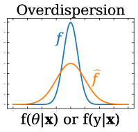
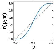
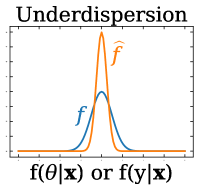
In Appendix C we describe Monte Carlo procedures for constructing confidence sets of $\widehat{r}^{\widehat{f}}(\gamma;{\mathbf{x}})$, and for testing the local null hypothesis $H_{0}({\mathbf{x}}):\widehat{F}(y|{\mathbf{x}})=F(y|{\mathbf{x}})\mbox{ for every }y\in\mathcal{Y}$.

2.2 Recalibration via P-P Map

Cal-PIT uses the estimated regression function $\widehat{r}^{\widehat{f}}(\gamma;{\mathbf{x}}):=\widehat{\mathbb{P}}\left({\rm PIT}(Y;{\mathbf{x}})\leq\gamma\ \middle|\ {\mathbf{x}}\right)$ to reshape the original CDE $\widehat{f}$, so that the recalibrated CDE $\widetilde{f}$ is approximately locally consistent across the feature space.

The procedure is as follows: Consider a fixed evaluation point ${\mathbf{x}}$ and any $y_{0}\in\mathcal{Y}$. Let $\gamma:=\widehat{F}(y_{0}|x)$. If the regression is perfectly estimated (that is, $\widehat{r}^{\widehat{f}}=r^{\widehat{f}}$), then, as long as both $F$ and $\widehat{F}$ are continuous and $\widehat{F}$ dominates $F$ (see Assumptions 1 and 2 in Section 3 for details),

$$r^{\widehat{f}}(\gamma;{\mathbf{x}}):= \mathbb{P}\left(\widehat{F}(Y|{\mathbf{x}})\leq\gamma\ \middle|\ {\mathbf{x}}\right)=\mathbb{P}\left(Y\leq y_{0}\ \middle|\ {\mathbf{x}}\right)$$

$$= F(y_{0}|{\mathbf{x}}).$$

That is, the regression function $r^{\widehat{f}}$ reshapes the initial CDE so that the probability of observing the response variable $Y$ below $y_{0}$ is now indeed $F(y_{0}|{\mathbf{x}})$ rather than $\widehat{F}(y_{0}|{\mathbf{x}})$, as illustrated by the right panel of Figure 1.

The above result suggests that we define a new conditional (cumulative) distribution function $\widetilde{F}$ with density $\widetilde{f}$:

Definition 3 (Recalibrated PD).

The recalibrated predictive distribution (PD) of $Y$ given ${\mathbf{x}}$ is defined through a P-P map,

$$\widetilde{F}(y|{\mathbf{x}}):=\widehat{r}^{\widehat{f}}\left(\widehat{F}(y|{\mathbf{x}});{\mathbf{x}}\right),$$ (6)

where $\widehat{r}^{\widehat{f}}$ is the regression estimator of the PIT-CDF (Equation 4).

Definition 4 (Estimated OT).

We define an estimate of the optimal transport from $\widehat{F}$ to $F$ by

$$\widehat{T}(y|{\mathbf{x}}):=\widetilde{F}^{-1}\left(\widehat{F}(y|{\mathbf{x}})|{\mathbf{x}}\right).$$ (7)

The rate of convergence of $\widetilde{F}(y|{\mathbf{x}})$ to the target distribution $F(y|{\mathbf{x}})$ is given by Corollary 1. Algorithm 1 details the Cal-PIT procedure for computing the PIT-CDF from calibration data, and for constructing recalibrated PDs, CDEs and prediction intervals. In practice, we employ a scheme where we, for each ${\mathbf{x}}$ of interest, first evaluate $\widetilde{F}(y|{\mathbf{x}})$ across a grid $G$ of $y$-values, and then use splines to interpolate between these values. By differentiating the spline functions, we finally obtain $\widetilde{f}(y|{\mathbf{x}})$, our estimate of the recalibrated CDE at ${\mathbf{x}}$.

The Cal-PIT prediction interval at ${\mathbf{x}}$, defined as

$$C_{\alpha}({\mathbf{x}}):=\left[\widetilde{F}^{-1}(0.5\alpha|{\mathbf{x}}),\ \widetilde{F}^{-1}(1-0.5\alpha|{\mathbf{x}})\right],$$ (8)

approximately achieves $1-\alpha$ conditional coverage. Alternatively, one may use Highest Predictive Density (HPD) sets, defined as $C_{\alpha}({\mathbf{x}})=\{y:\widetilde{f}(y|{\mathbf{x}})\geq\widetilde{t}_{{\mathbf{x}},\alpha}\}$, where $\widetilde{t}_{{\mathbf{x}},\alpha}$ is such that $\int_{y\in C_{\alpha}({\mathbf{x}})}\widetilde{f}(y|{\mathbf{x}})dy=1-\alpha$ and $\widetilde{f}$ is the density associated to $\widetilde{F}$. HPD regions can produce more informative and considerably smaller prediction sets than intervals for multimodal and skewed densities. See Appendix B for additional details.

Algorithm 1 Cal-PIT

Require: initial CDE $\widehat{f}(y|{\mathbf{x}})$ evaluated at $y\in G$; calibration set $\mathcal{D}=\{({\mathbf{X}}_{1},Y_{1}),\ldots,({\mathbf{X}}_{n},Y_{n})\}$; oversampling factor $K$; evaluation points $\mathcal{V}\subset\mathcal{X}$; nominal miscoverage level $\alpha$, flag HPD (true if computing HPD sets)
Ensure: recalibrated PD $\widetilde{F}(y|{\mathbf{x}})$, Cal-PIT interval $C({\mathbf{x}})$, recalibrated CDE $\widetilde{f}(y|{\mathbf{x}})$, for all ${\mathbf{x}}\in\mathcal{V}$

1:// Learn PIT-CDF from augmented and upsampled calibration data $\mathcal{D^{\prime}}$

2:Set $\mathcal{D^{\prime}}\leftarrow\emptyset$

3:for $i$ in $\{1,...,n\}$ do

4:     for $j$ in $\{1,...,K\}$ do

5:         Draw $\gamma_{i,j}\sim U(0,1)$

6:         Compute $W_{i,j}\leftarrow{\mathbb{I}}\left({\rm PIT}(Y_{i};{\mathbf{X}}_{i})\leq\gamma_{i,j}\right)$

7:         Let $\mathcal{D^{\prime}}\leftarrow\mathcal{D^{\prime}}\cup\{\left({\mathbf{X}}_{i},\gamma_{i,j},W_{i,j}\right)\}$

8:     end for

9:end for

10:Use $\mathcal{D^{\prime}}$ to learn $\widehat{r}^{\widehat{f}}(\gamma;{\mathbf{x}}):=\widehat{\mathbb{P}}\left({\rm PIT}(Y;{\mathbf{x}})\leq\gamma\ \middle|\ {\mathbf{x}}\right)$ via a regression of $W$ on ${\mathbf{X}}$ and $\gamma$, which is monotonic w.r.t. $\gamma$.

11:

12:// Recalibration using PIT-CDF as a P-P map

13:for ${\mathbf{x}}\in\mathcal{V}$  do

14:     // Construct recalibrated PD and CDE

15:     Compute $\widehat{F}(y|{\mathbf{x}})\leftarrow\mathrm{cumsum}(\widehat{f}(y|{\mathbf{x}}))$ for $y\in G$

16:     Let $\widetilde{F}(y|{\mathbf{x}})\leftarrow\widehat{r}^{\widehat{f}}\left(\widehat{F}(y|{\mathbf{x}});{\mathbf{x}}\right)$ for $y\in G$

17:     Apply interpolating (or smoothing) splines to obtain $\widetilde{F}(\cdot|{\mathbf{x}})$ and $\widetilde{F}^{-1}(\cdot|{\mathbf{x}})$

18:     Differentiate $\widetilde{F}(y|{\mathbf{x}})$ to obtain recalibrated CDE $\widetilde{f}(y|{\mathbf{x}})$ for $y\in G$

19:     Renormalize $\widetilde{f}(y|{\mathbf{x}})$ according to Izbicki and Lee (2016, Section 2.2)

20:     

21:     // Construct Cal-PIT interval with conditional coverage $1-\alpha$

22:     Compute $C({\mathbf{x}})\leftarrow[\widetilde{F}^{-1}(0.5\alpha|{\mathbf{x}});\widetilde{F}^{-1}(1-0.5\alpha|{\mathbf{x}})]$.

23:     if HPD then

24:         Obtain HPD sets $C({\mathbf{x}})=\{y:\widetilde{f}(y|{\mathbf{x}})\geq\widetilde{t}_{{\mathbf{x}},\alpha}\}$, where $\widetilde{t}_{{\mathbf{x}},\alpha}$ is such that $\int_{y\in C_{\alpha}({\mathbf{x}})}\widetilde{f}(y|{\mathbf{x}})dy=1-\alpha$

25:     end if

26:end for

27:return $\widetilde{F}(y|{\mathbf{x}})$, $C({\mathbf{x}})$, $\widetilde{f}(y|{\mathbf{x}})$, for all ${\mathbf{x}}\in\mathcal{V}$

Remark 2.

If the initial model is good, then $r$ is easy to estimate; for instance, $\widehat{f}=f$ implies a constant function $r^{\widehat{f}}(\gamma;{\mathbf{x}})=\gamma$. However, $\widehat{f}$ needs to be supported on the entire feature space $\mathcal{X}$. Depending on the application, a viable initial model could, for example, be a uniform distribution on finite support (as in Experiment 2 of Section 4.1), an estimate of the marginal distribution $f(y)$ (as in the photo-z application in Section 5.1), or an initial fit of the density with an MDN with a wide Gaussian distribution (as in the TC application in Section 5.2).

3 Theoretical Properties

Next, we show how the performance of the recalibrated PD estimator $\widetilde{F}$ relates to the mean squared error of the regression function $\widehat{r}^{\widehat{f}}$, and provide convergence rates. We also show that Cal-PIT intervals achieve asymptotic conditional validity even if the initial CDE $\widehat{f}$ is not consistent. The following results are conditional on $\widehat{f}$; all uncertainty refers to the calibration sample. We assume that the true distribution of $Y|{\mathbf{x}}$ and its initial estimate are continuous, and that $\widehat{F}$ places its mass on a region that is at least as large as that of $F$:

Assumption 1 (Continuity of the cumulative distribution functions).

For every ${\mathbf{x}}\in\mathcal{X}$, $\widehat{F}(\cdot|{\mathbf{x}})$ and $F(\cdot|{\mathbf{x}})$ are continuous functions.

Assumption 2 ($\widehat{F}$ dominates $F$).

For every ${\mathbf{x}}\in\mathcal{X}$, $\widehat{F}(\cdot|{\mathbf{x}})$ dominates $F(\cdot|{\mathbf{x}})$.

We also assume that $F(\cdot|{\mathbf{x}})$ cannot place too much mass in regions where the initial estimate $\widehat{F}(\cdot|{\mathbf{x}})$ places little mass:

Assumption 3 (Bounded density).

There exists $K>0$ such that, for every ${\mathbf{x}}\in\mathcal{X}$, the Radon-Nikodym derivative of $F(\cdot|{\mathbf{x}})$ with respect to $\widehat{F}(\cdot|{\mathbf{x}})$ is bounded above by $K$.

Under the above assumptions, we can relate the performance of the recalibrated PD with the performance of the regression function:

Theorem 1 (Performance of the recalibrated PD).

Under Assumptions 1, 2 and 3,

$${\mathbb{E}}\left[\int\int\left(\widetilde{F}(y|{\mathbf{x}})-F(y|{\mathbf{x}})\right)^{2}dP(y,{\mathbf{x}})\right]=K{\mathbb{E}}\left[\int\int\left(\widehat{r}^{\widehat{f}}(\gamma;{\mathbf{x}})-r^{\widehat{f}}(\gamma;{\mathbf{x}})\right)^{2}d\gamma dP({\mathbf{x}})\right].$$

To provide rates of convergence for the recalibrated PD, we will in addition assume that the regression method converges at a rate $O(n^{-\kappa})$:

Assumption 4 (Convergence rate of the regression method).

The regression method used to estimate $r^{\widehat{f}}$ is such that its convergence rate is given by

$${\mathbb{E}}\left[\int\int\left(\widehat{r}^{\widehat{f}}(\gamma;{\mathbf{x}})-r^{\widehat{f}}(\gamma;{\mathbf{x}})\right)^{2}d\gamma dP({\mathbf{x}})\right]=O\left(\frac{1}{n^{\kappa}}\right)$$

for some $\kappa>0$.

Many methods satisfy Assumption 4 for some value $\kappa$, which is typically rated to the dimension of $\mathcal{X}$ and the smoothness of the true regression $r$ (see for instance Györfi et al. 2002).

Under these assumptions, we can derive the rate of convergence for $\widetilde{F}$:

Corollary 1 (Convergence rate of recalibrated PD).

Under Assumptions 1, 2, 3 and 4,

$${\mathbb{E}}\left[\int\int\left(\widetilde{F}(y|{\mathbf{x}})-F(y|{\mathbf{x}})\right)^{2}dP(y,{\mathbf{x}})\right]=O\left(\frac{1}{n^{\kappa}}\right).$$

Next, we show that with an uniformly consistent regression estimator $\widehat{r}^{\widehat{f}}(\gamma;{\mathbf{x}})$ (see Bierens 1983; Hardle et al. 1984; Liero 1989; Girard, Guillou and Stupfler 2014 for some examples), Cal-PIT intervals achieve asymptotic conditional validity, even if the initial CDE $\widehat{f}(y|{\mathbf{x}})$ is not consistent.

Assumption 5 (Uniform consistency of the regression estimator).

The regression estimator is such that

$$\sup_{{\mathbf{x}}\in\mathcal{X},\gamma\in[0,1]}|\widehat{r}^{\widehat{f}}(\gamma;{\mathbf{x}})-r^{\widehat{f}}(\gamma;{\mathbf{x}})|\xrightarrow[n\longrightarrow\infty]{\enskip\text{a.s.}\enskip}0,$$

where the convergence is with respect to the calibration set $\mathcal{D}$ only; $\widehat{f}$ is fixed.

Theorem 2 (Consistency and conditional coverage of Cal-PIT intervals).

Let $C^{*}_{\alpha}({\mathbf{x}})=\left[F^{-1}(0.5\alpha|{\mathbf{x}});F^{-1}(1-0.5\alpha|{\mathbf{x}})\right]$ be the oracle prediction band, and let $C^{n}_{\alpha}({\mathbf{x}})$ denote the Cal-PIT interval. Under Assumptions 1, 2 and 5,

$$\lambda\left(C_{\alpha}^{n}({\mathbf{X}})\Delta C_{\alpha}^{*}({\mathbf{X}})\right)\xrightarrow[n\longrightarrow\infty]{\enskip\text{a.s.}\enskip}0,$$

where $\lambda$ is the Lebesgue measure in $\mathbb{R}$ and $\Delta$ is the symmetric difference between two sets. It follows that $C_{\alpha}^{n}({\mathbf{X}})$ has asymptotic conditional coverage of $1-\alpha$ (Lei et al., 2018).

See Appendix D.1 for theoretical results for Cal-PIT(HPD).

4 Synthetic Examples

4.1 Example 1: IID Data. No Model Misspecification

In photo-z estimation, multiple widely different distances (redshift) can be consistent with the observed features (colors) of a galaxy. This, as mentioned, results in PDs that are multimodal in parts of the feature space. Motivated by the photo-z application, we have modified the two-group example of Feldman, Bates and Romano (2021) to have bimodal structure due to limited predictor information. Here the target variable $Y$ depends on three variables: $X_{0},X_{1},X_{2}$. Variable $X_{0}$ indicates group membership but it is not measured; that is, $X_{1}$ and $X_{2}$ are our only predictors. The missing membership information results in the CDE $f(y|x_{1},x_{2})$ being bimodal in the regime $X_{1}>0$ with one branch corresponding to each class. Appendix Conditionally Calibrated Predictive Distributions by Probability-Probability Map: Application to Galaxy Redshift Estimation and Probabilistic Forecasting details the data-generating process (DGP), and Figure 3 visualizes one random instance of data drawn from $f(y|x_{1},x_{2})$ with the “majority” and “minority” groups displayed as blue versus orange points.

Our primary goal is to calibrate entire PDs, but because of the rich recent literature on calibrated prediction sets, we design two experiments for benchmarking Cal-PIT prediction sets against results from conformal inference, quantile regression and normalizing flows:

• Experiment 1 (comparison with conformal inference): For this experiment, we split a sample of total size $n$ in two halves: the first half is used to train an initial model, the second half is used for calibration.

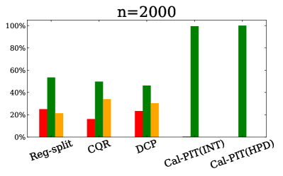
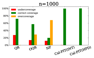
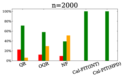
  The empirical coverage of the final prediction sets are computed via $1000$ Monte Carlo (MC) simulations from the true DGP at each test point on a grid. Test points with coverage within two standard deviations (SD) of the nominal coverage of $1-\alpha=0.9$ based on 100 random realizations are labeled as having “correct” coverage. We report the proportion of test points in the feature space with “under-”, “correct”, versus “over-” coverage.

• Experiment 2 (comparison with quantile regression and normalizing flows): Here we use the entire sample of size $n$ to compute quantiles or to estimate the conditional density. As above, we use MC simulations on a grid to assess conditional coverage.

The top row of Figure 4 shows results for Experiment 1. We compare $90\%$ prediction sets for $Y$ using Cal-PIT(INT) and Cal-PIT(HPD) with prediction sets from Reg-split (Lei et al., 2018), conformalized quantile regression (CQR; Romano, Patterson and Candès 2019), and distributional conformal prediction (DCP; Chernozhukov, Wüthrich and Zhu 2021). Reg-split and CQR are trained with XGBoost (Chen and Guestrin, 2016). Our Cal-PIT methods use an initial CDE trained using FlexCode with an XGBoost regressor (Izbicki and Lee, 2017; Dalmasso et al., 2020a) and monotonic neural networks (Wehenkel and Louppe, 2019) for learning $\widehat{r}^{\widehat{f}}(\gamma;{\mathbf{x}})$ with a mean-squared-error loss. DCP computes a conformal score based on PIT values derived from the same initial CDE as Cal-PIT. All methods improve in terms of conditional coverage with increasing sample size, but only Cal-PIT consistently attains the nominal $90\%$ coverage across the feature space for $n\geq 2000$.

The bottom row of Figure 4 shows results for Experiment 2. Cal-PIT (INT) and Cal-PIT (HPD) reshape a uniform distribution on ${\mathbf{x}}\in[-5,5]$; hence, there is no need for a separate training set. The Cal-PIT prediction sets are then compared to output from quantile regression (QR; Koenker and Bassett Jr. 1978) trained with XGBoost and a pinball loss, orthogonal quantile regression (OQR; Feldman, Bates and Romano 2021) which introduces a penalty on the pinball loss to improve conditional coverage, and normalizing flows (NF). We use the PZFlow (Crenshaw, Yan and vladislav doster, 2023) implementation of Normalizing Flows which has been optimized to work well out-of-the-box with tabular data and uses Neural Spline Flows (Dinh, Krueger and Bengio, 2014; Dinh, Sohl-Dickstein and Bengio, 2016; Durkan et al., 2019) as the backbone.

Figure 3: Visualization of one random instance of the data used for Example 1. There are two covariates ($X_{1},X_{2}$), and a target variable $Y$. The analytic form of the true data distribution is defined in Appendix Conditionally Calibrated Predictive Distributions by Probability-Probability Map: Application to Galaxy Redshift Estimation and Probabilistic Forecasting. The data set consists of two groups with different spreads. $Y$ splits into two branches for $X_{1}>0$; that is, the true CDE is bimodal in this region.

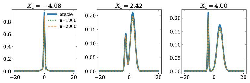
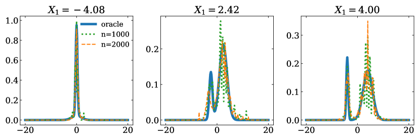
Figure 5a, top row, shows some examples of calibrated CDEs from Cal-PIT. The estimates reveal that the true conditional density is bimodal for $X_{1}>0$; thus, the most efficient prediction sets in this feature subspace would not be single intervals, but rather pairs of intervals. Indeed, Cal-PIT (HPD) yields smaller prediction sets than Cal-PIT (INT); see Fig. 15 in Supplementary Material. Because HPD sets can capture the bimodality in the data while intervals cannot, this is a case where Cal-PIT (HPD) has better efficiency. This qualitative insight is only possible because Cal-PIT estimates the entire PDs. Normalizing flows also provide entire CDEs (see Figure 5b, bottom row) but can be difficult to train.

(a)

(b)

Figure 4: The proportion of test points with correct conditional coverage for (a) “Experiment 1” with state-of-the-art conformal inference methods, using data of total size $n$ split into a train and a calibration set, and (b) “Experiment 2” with quantile regression and normalizing flow approaches, which use all data for training. See text for details. Only Cal-PIT consistently attains the nominal $90\%$ coverage across the feature space with increasing sample size $n$.

(a) CDEs from Cal-PIT

(b) CDEs from Normalizing Flows

Figure 5: CDEs at three different values of $X_{1}$ ($X_{2}=0$) for (a) Cal-PIT and (b) Normalizing Flows for “Experiment 2”. The results for $n=1000$ and $n=2000$ are compared to the “oracle” probability density functions.

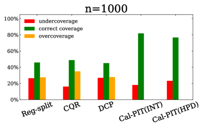
4.2 Example 2: Misspecified Models

Conformal inference methods can perform poorly if the initial model is misspecified. Cal-PIT will, on the other hand, by construction attempt to morph the initial density into the density of the calibration data. This property is, for example, useful for settings with distributional shift. Here we show what the morphing of densities by diagnostic ALPs might look like for a synthetic example with a single predictor $X$. The original model is trained on data $\mathcal{T}=\{(X_{1},Y_{1}),...,(X_{n},Y_{n})\}$ from a Gaussian conditional density,

$$Y|X\sim\mathcal{N}(\mu=X,\sigma=2),$$

but the target has a distribution that is either skewed with

$$Y_{A}|X\sim\text{sinh-arcsinh}(\mu=X,\sigma=2-|X|,\gamma=X,\tau=1),$$

or kurtotic with

$$Y_{B}|X\sim\text{sinh-arcsinh}(\mu=X,\sigma=2,\gamma=0,\tau=1-X/4).$$

In both settings, we have access to calibration data $\mathcal{D}=\{({\mathbf{X}}^{\prime}_{1},Y^{\prime}_{1}),...,({\mathbf{X}}^{\prime}_{n},Y^{\prime}_{n})\}$ from the true target distribution. We use monotonic neural networks to learn the PIT-CDF, $\widehat{r}^{\widehat{f}}$ for $n=10000$. The final coverage is assessed via MC simulations from the true DGP.

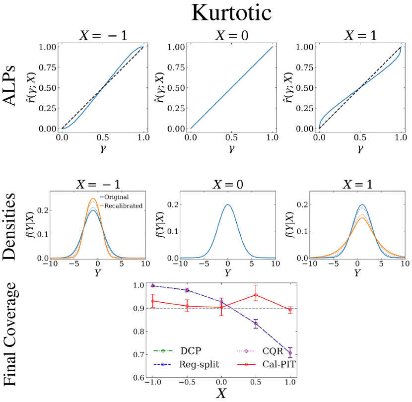
Figure 3, top row, shows diagnostic ALPs at three different evaluation points of $X$ for the “skewed” setting. These plots provide information on how the estimated conditional density $\widehat{f}(y|x)$ deviates from the true density $f(y|x)$ at the evaluation points. In addition, the function $\widehat{r}^{\widehat{f}}$ itself provides us with an approximation of the entire optimal transport map from $\widehat{f}(y|x)$ to $f(y|x)$ at any ${\mathbf{x}}$; the second row shows examples of morphing of the initial density (blue color) into the recalibrated density (orange color) via Cal-PIT.

The bottom row of Figure 6 shows that the PDs are approximately calibrated after reshaping the densities via Cal-PIT whereas reg-split, CQR and DCP fail to achieve conditional coverage when the initial model is mis-specified, even though the densities are recalibrated using data from the true data-generating process. Finally, our method is the only one that pinpoints the nature of the discrepancy from the estimated distribution and then directly corrects for deviations in conditional coverage. Figure 7 showcases similar results for the “kurtotic” setting.

Figure 6: The initial fit is Gaussian, but the target distribution is skewed, so the model is misspecified. Top: Diagnostic ALPs. Cal-PIT identifies that the model is positively/negative biased relative to calibration data at $X=-1$/$X=1$ but well estimated at $X=0$. The diagnostics define P-P maps for reshaping the initial densities so as to fit calibration data across the feature space. Center: Morphing of densities via Cal-PIT. Bottom: Empirical coverage for different calibration methods; nominal coverage level $1-\alpha=0.9$. Cal-PIT is the only method to achieve approximate conditional calibration for all inputs $X$ when the initial model is misspecified due to a distributional shift.

Figure 7: Left: The initial fit is Gaussian, but the target distribution is kurtotic, so the model is misspecified. Top: Diagnostic ALPs. Cal-PIT identifies that the model is over/under-dispersed relative to the calibration data at $X=-1$/$X=1$ but well estimated at $X=0$. The diagnostics define P-P maps for reshaping the initial densities so as to fit calibration data across the feature space. Center: Morphing of densities via Cal-PIT. Bottom: Empirical coverage for different calibration methods; nominal coverage level $1-\alpha=0.9$. Cal-PIT is the only method to achieve approximate conditional calibration for all inputs $X$ when the initial model is misspecified due to a distributional shift.

5 Applications

5.1 Calibrating CDEs of Galaxy Photometric Redshift

Our main application is the problem of estimating CDEs for galaxy photometric redshifts.

As images contain limited information about redshifts, galaxies at very different redshifts can have similar image properties, resulting in, e.g., complex multi-modal distributions that are not well summarized by point estimates or standard probability distributions

(Benítez, 2000; Mandelbaum et al., 2008; Malz and Hogg, 2022).

When sufficient training data are available, machine learning-based techniques are widely utilized for predicting photo-$z$ distributions (e.g., Beck et al. 2016; Zhou et al. 2021; Dalmasso et al. 2020a; Almosallam, Jarvis and Roberts 2016; Dey et al. 2021). However, these methods do not guarantee accurate coverage.

As a solution, previous studies, such as Bordoloi, Lilly and Amara (2010); Euclid Collaboration et al. (2021), have employed PIT-based recalibration schemes for photo-$z$ CDEs to enforce marginal coverage. In contrast, our approach focuses on the more stringent requirement of achieving satisfactory conditional coverage.

Here we use the data set from Schmidt et al. (2020),

which has previously been employed as a benchmark for evaluating photo-$z$ CDE prediction methods. The features used to train the models are called apparent magnitudes and colors which are various measures of total light in an image. For our calibration set, we employ the “training set” described in Schmidt et al. (2020), comprising approximately 44,000 instances, and we adopt the same test set as the aforementioned study.

We apply Cal-PIT by recalibrating trainZ (Schmidt et al., 2020), which is an estimate of the marginal distribution of redshifts. Although this naive estimate does not contain any meaningful information about individual redshifts, Schmidt et al. (2020) demonstrated that

it can perform well on many commonly used metrics that check for marginal coverage.

Figure 8: Top: Diagnostic ALPs for five galaxies before recalibration. Center: Photo-$z$ CDEs for the corresponding galaxies before and after using Cal-PIT along with their true redshifts. We see that we can recover bimodal CDEs even if our initial estimate was not bimodal. Bottom: Comparison of the CDEs with the distribution of true redshifts of other galaxies having similar imaging properties. We observe that the histograms show bimodal distributions only when our inferred CDEs are bimodal.

We train $r^{\widehat{f}}$ on the calibration data and use Cal-PIT to recalibrate the CDEs of our validation and test sets. We assess the quality of our recalibrated CDEs with the Conditional Density Estimate (CDE) loss (Izbicki and Lee, 2017), a metric of conditional coverage that is independent of Cal-PIT and also employed in the Schmidt et al. (2020) benchmark study. The CDE loss is an analog of the root-mean-square-error. Given an estimate $\widetilde{f}$ of $f$, it is defined as

$$L(f,\widetilde{f})=\int\int[f(y|\mathbf{x}-\widetilde{f}(y|\mathbf{x}))]^{2}\mathrm{d}y\mathrm{d}P(\mathbf{x})$$

where $\mathrm{d}P(\mathbf{x})$ is the marginal distribution of features $\mathbf{x}$. The CDE loss cannot be evaluated directly as it depends on the unknown true density $f(y|\mathbf{x})$ but it can be estimated up to a constant ($K_{f}$; dependent on $f(y|\mathbf{x})$) by

$$\widehat{L}(f,\widetilde{f})={\mathbb{E}}_{\mathbf{x}}\left[\int\widetilde{f}(y|\mathbf{x})^{2}\mathrm{d}y\right]-2{\mathbb{E}}_{\mathbf{x},y}\left[\widetilde{f}(y|\mathbf{x})\right]+K_{f}$$

We infer the local CDF of PIT for every instance in the test set using the trained model. Fig. 8 (top) shows the diagnostic ALPs applied to the original estimate, $\widehat{f}(y)$, for a few galaxies in the test set. Even though the marginal PIT distribution follows the identity line closely, our ALPs are able to show that $\widehat{f}(y)$ is not a good estimate: the local CDF of PIT for these instances deviates significantly from the identity line.

Figure 8 (center) shows that multimodal CDEs can be recovered, even when the input CDE before calibration is unimodal.

Since we do not know the “ground truth” distributions, we generally have to rely on indirect methods to assess coverage. Fig. 8 (bottom) provides a rudimentary but direct demonstration that the CDEs from Cal-PIT are indeed meaningful. In the figure, we compare the CDEs with the distribution of true redshifts of other galaxies with similar imaging data. We identify those counterparts by searching for other galaxies in the training set whose colors and magnitudes (rescaled by subtracting the mean and dividing by the standard deviation for each feature) lie within a Euclidean distance of 0.5 units of our selected galaxies. Fig. 8 (bottom) shows their redshift distribution as an inverse-distance weighted histogram along with their predicted CDEs. We observe that the histograms show bimodal distributions when our inferred CDEs are bimodal, and unimodal when the inferred distribution is unimodal, matching astronomers’ expectations. Finally, Table 1 shows that Cal-PIT yields lower CDE loss than any of the methods in the LSST-DESC data challenge (Schmidt et al., 2020).

In particular, there is a large improvement in the value of the CDE loss, with a decrease from $-0.84$ to $-10.71$ after recalibration.

Table 1: Comparison with methods benchmarked in the LSST-DESC Photo-z Data Challenge (Schmidt et al., 2020). In terms of CDE loss, Cal-PIT performs better than all the other methods compared, including one approach which was specifically optimized for minimum CDE loss (FlexZBoost).

Photo-$z$ Algorithm	CDE Loss
ANNz2 (Sadeh, Abdalla and Lahav, 2016)	-6.88
BPZ (Benítez, 2000)	-7.82
Delight (Leistedt and Hogg, 2017)	-8.33
EAZY (Brammer, van Dokkum and Coppi, 2008)	-7.07
FlexZBoost (Izbicki and Lee, 2017)	-10.60
GPz (Almosallam, Jarvis and Roberts, 2016)	-9.93
LePhare (Arnouts et al., 1999)	-1.66
METAPhoR (Cavuoti et al., 2017)	-6.28
CMNN (Graham et al., 2018)	-10.43
SkyNet (Graff et al., 2014)	-7.89
TPZ (Carrasco Kind and Brunner, 2013)	-9.55
trainZ (Schmidt et al., 2020)	-0.83
Cal-PIT	-10.71

5.2 Probabilistic Nowcasting for Dependent High-Dimensional Data

Our next example is a toy version of TC intensity forecasting based on infrared (IR) satellite image data. This application is challenging both because of the high-dimensional nature of the image data, and because of observations being correlated in time.

Figure 9, right, shows an example of a 24-hour sequence $\mathbf{S}_{<t}$ of consecutive radial profiles (one-dimensional functions) extracted from Geostationary Operational Environmental Satellite (GOES) IR imagery (Janowiak, Joyce and Xie, 2020); see Appendix Conditionally Calibrated Predictive Distributions by Probability-Probability Map: Application to Galaxy Redshift Estimation and Probabilistic Forecasting for details. IR imagery as observed by GOES measures the cloud-top temperature, which is a proxy of the strength of convection (the key component of the mechanism through which TCs extract energy from the ocean). Hence, each computed sequence $\mathbf{S}_{<t}$ can be seen as a summary of the spatio-temporal evolution of TC convective structure leading up to time $t$. This 24-hour trajectory is closely related to the current storm intensity. Our objective is to “nowcast” the PD $Y_{t}|\mathbf{S}_{<t}$, where $Y_{t}$ is the TC intensity at time $t$.

Figure 9: Left: A sequence of TC-centered cloud-top temperature images from GOES. Center: We represent each GOES image with a radial profile of azimuthally-averaged cloud-top temperatures. Right: The 24-hour sequence of consecutive radial profiles, sampled every 30 minutes, defines a structural trajectory $\mathbf{S}_{<t}$ or Hovmöller diagram. Figure adapted from McNeely et al. (2022).

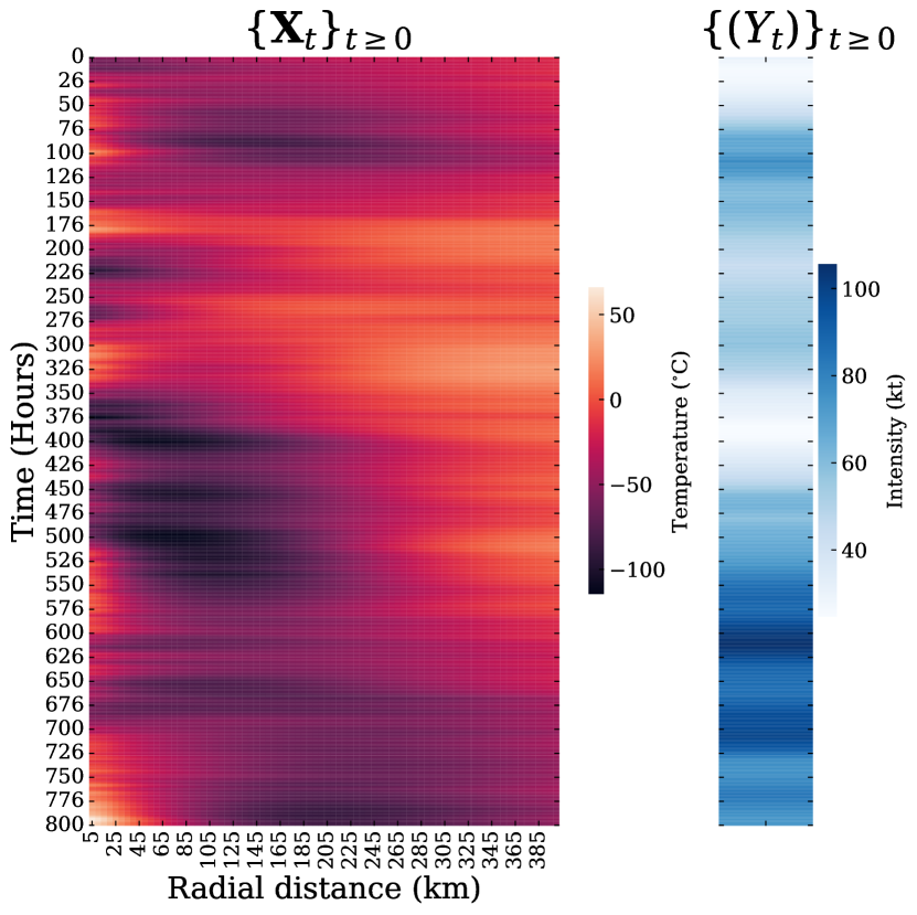
For the purposes of methods assessment via MC samples, we create a toy generative model based on TC intensity and location data from the NHC’s HURDAT2 best track database (Landsea and Franklin, 2013), and GOES longwave infrared imagery from NOAA’s MERGIR database (Janowiak, Joyce and Xie, 2020) of storms from the North Atlantic and Eastern North Pacific basins between 2000-2020: First, we fit a vector auto-regressive model to the principal components of radial profiles computed on historical data. Then, we simulate a series of scalar TC intensities $Y_{t}$ via a time series regression of $Y_{t}$ on its own most recent values and on $\mathbf{S}_{<t}$. The details are described in Appendix Conditionally Calibrated Predictive Distributions by Probability-Probability Map: Application to Galaxy Redshift Estimation and Probabilistic Forecasting. Figure 10 shows an example of a simulated storm. On the left, we have a toy Hovmöller diagram of the evolution of TC convective structure $\{({\mathbf{X}}_{t})\}_{t\geq 0}$, with each row representing the radial profile ${\mathbf{X}}_{t}\in\mathbb{R}^{120}$ of cloud-top temperatures as a function of radial distance from the TC center; time evolution is top-down in hours. On the right, we have $\{Y_{t}\}_{t\geq 0}$, the simulated TC intensities at corresponding times $t$. The trajectory $\mathbf{S}_{<t}:=({\mathbf{X}}_{t-48},{\mathbf{X}}_{t-47},\ldots,{\mathbf{X}}_{t})$ represents the 24-hour history of convective structure (49 radial profiles). We simulate 800 “storms” according to a fitted TC length distribution. Sequence data $\{(\mathbf{S}_{<t},Y_{t})\}$ from the same storm are shifted by 30 minutes; hence, they are strongly correlated. Sequence data from different storms, on the other hand, are independent.

Figure 10: Simulated radial profiles and intensities for an example TC. Left: Hovmöller diagram of the evolution of TC convective structure $\{{\mathbf{X}}_{t}\}_{t\geq 0}$; each row represents the radial profile ${\mathbf{X}}_{t}$ of cloud-top temperatures as a function of radial distance from the TC center at time $t$. Our predictors are 48-hour overlapping sequences $\{\mathbf{S}_{t}\}_{t\geq 0}$ with data from the same “storm” being highly dependent. Right: The target response, here shown as a time series $\{(Y_{t})\}_{t\geq 0}$ of simulated TC intensities.

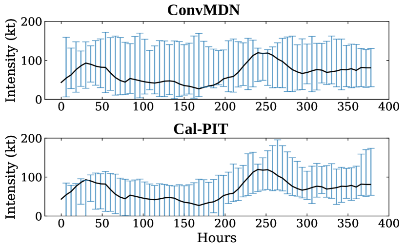
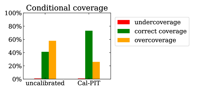
Our goal is to construct prediction sets for $Y_{t}|\mathbf{S}_{<t}$. Here we illustrate how Cal-PIT can improve upon an initial MDN fit. In our example, we perform training, calibration, and testing on different simulated “storms”: First, we fit an initial CDE (ConvMDN; D’Isanto and Polsterer 2018), which estimates $f(y|{\mathbf{s}})$ as a unimodal Gaussian, based on a train set with 8000 points, $\{(\mathbf{S}_{<t},Y_{t})\}$ (see Appendix Conditionally Calibrated Predictive Distributions by Probability-Probability Map: Application to Galaxy Redshift Estimation and Probabilistic Forecasting for details). Next, we apply Cal-PIT to learn $\widehat{r}^{\widehat{f}}(\gamma;{\mathbf{s}})$ using 8000 calibration points. (Note that the the data within the same storm are highly dependent; hence, the effective train or calibration sample sizes are much smaller than the nominal values.) Finally, we evaluate the conditional coverage of the initial CDE and Cal-PIT on MC samples at 4000 test points.

Fig. 11 summarizes the results. Cal-PIT recalibration improves upon the initial ConvMDN fit: The left panel displays prediction sets for $Y_{t}|\mathbf{S}_{<t}$ for a sample simulated TC, before and after calibration. The calibrated prediction sets track the behavior of the observed trajectory more closely (see Appendix Conditionally Calibrated Predictive Distributions by Probability-Probability Map: Application to Galaxy Redshift Estimation and Probabilistic Forecasting for more examples). The right panel illustrates that Cal-PIT also achieves better conditional coverage, even though the effective sample size is small due to dependencies between intensities in the same storm.

(a)

(b)

Figure 11: Left: Simulated TC example with dependent high-dimensional sequence data. Prediction sets for TC intensities, before and after calibration (blue bars), together with the actual trajectory of intensities $\{Y_{t}\}_{t}$ (solid black lines). Cal-PIT tracks the behavior of the trajectories more closely. Right: Conditional coverage of both methods across sequences ${\mathbf{s}}$. The initial ConvMDN fit with a single Gaussian component over-covers in certain regions of the feature space due to the true PD being skewed toward larger intensities (Appendix  Conditionally Calibrated Predictive Distributions by Probability-Probability Map: Application to Galaxy Redshift Estimation and Probabilistic Forecasting); Cal-PIT partly corrects for the over-coverage and returns more precise prediction sets.

6 Discussion

Whereas there are few reliable estimators for conditional densities or quantile regression, there is a large literature devoted to estimating regression functions. Our approach draws upon the success of high-capacity predictive algorithms, such as deep neural networks, to recalibrate PDs in complex data settings with a minimum of assumptions.

Cal-PIT can assess whether a PD estimate $\widehat{F}(\cdot|{\mathbf{x}})$ is well-calibrated for all inputs ${\mathbf{x}}$, as well as correct for discrepancies. In order for Cal-PIT corrections to give good results, the initial estimate $\widehat{F}(\cdot|{\mathbf{x}})$ needs to place its mass on a region which is at least as large as $F(\cdot|{\mathbf{x}})$, but the initial fit can be poor otherwise. Good results also require calibration data to learn the regression function (Eq. 4); empirically, we see that data sizes are still reasonable if using the right NN architecture and training correctly. Cal-PIT does not require exchangeable data, only stationary processes; hence it can be applied to (stationary) probabilistic time series forecasting. Individually calibrated PDs automatically return conditionally calibrated prediction sets. However, Cal-PIT works under the assumption that $Y$ is continuous and does not apply to classification tasks (unlike calibration schemes in, e.g., Kull et al. 2019; Wald and Globerson 2017).

Finally, Cal-PIT can potentially be extended to multivariate output vectors ${\mathbf{Y}}$ by the decomposition $f({\mathbf{y}}|{\mathbf{x}})=\prod_{i}f(y_{i}|{\mathbf{x}},{\mathbf{y}}_{<i})$; thus performing Cal-PIT corrections on auto-regressive components of the conditional distribution. This is a particularly promising direction for Deep Pixel-CNN and Pixel-RNN models (Van den Oord et al., 2016; van den Oord and Kalchbrenner, 2016). We are currently investigating whether Cal-PIT can improve structural forecasts for short-term tropical cyclone intensity guidance (McNeely et al., 2023). See also Linhart, Gramfort and Rodrigues (2022) for a multivariate extension specific to normalizing flows. Other open problems include fast sampling from recalibrated PDs to generate ensemble forecasts in real time.

See Supplementary Material for “Details on Example 1”, “Training a regression model to learn $\widehat{r}^{\widehat{f}}(\gamma;{\mathbf{x}})$”, and “Details on probabilistic nowcasting application”.

Appendix A Optimal Transport

Here we briefly review Monge’s continuous formulation of the OT distance; please consult Villani (2021) for a more complete and mathematical description of OT.

Consider two distributions $F_{0}$ and $F$ defined over respective domains $\Omega_{0},\Omega\subseteq\mathbb{R}^{d}$. Monge’s OT problem is to find a function $T:\Omega_{0}\rightarrow\Omega$ that pushes $F_{0}$ onto $F$ and minimizes the distance

$$d(F_{0},F)=\inf_{T}\int\|{\mathbf{x}}-T({\mathbf{x}})\|^{p}dF_{0}({\mathbf{x}})$$

subject to $T({\mathbf{X}})\sim F$, where $p\geq 1$ and ${\mathbf{X}}\sim F_{0}$. Such a minimizer $T^{*}$ exists if $F_{0}$ and $F$ both have densities. The minimizer $T^{*}$ is called the optimal transport map. The map $T_{t}({\mathbf{x}})=(1-t){\mathbf{x}}+tT^{*}({\mathbf{x}})$, for $t\in[0,1]$, gives the path of a particle of mass at ${\mathbf{x}}$. The distribution of $T_{t}({\mathbf{X}})$ is also the geodesic (that is, the shortest path according to the metric $d$) connecting $F_{0}$ to $F$; see Kolouri et al. (2017) for a technical definition.

If $\Omega=\Omega_{0}=\mathbb{R}$ and both $F$ and $F_{0}$ are absolutely continuous, with continuous densities which do not vanish, the optimal transport is given by

$$T(x)=F^{-1}\left(F_{0}(x)\right).$$

See Santambrogio (2015) for a detailed survey.

Appendix B Cal-PIT (HPD) and Cal-HPD

Cal-PIT (HPD) Cal-PIT can also be used to compute Highest Predictive Density regions (HPDs) instead of prediction intervals. The oracle (1-$\alpha$)-level HPD set is defined as

$$\text{HPD}_{\alpha}({\mathbf{x}})=\{y:f(y|{\mathbf{x}})\geq t_{{\mathbf{x}},\alpha}\},$$

where $t_{{\mathbf{x}},\alpha}$ is such that $\int_{y\in\text{HPD}_{\alpha}({\mathbf{x}})}f(y|{\mathbf{x}})dy=1-\alpha$. HPDs are the smallest prediction sets that have coverage $1-\alpha$, and thus they may be more precise (smaller set size) than quantile-based intervals, while maintaining the conditional coverage at the nominal level (see Appendix Conditionally Calibrated Predictive Distributions by Probability-Probability Map: Application to Galaxy Redshift Estimation and Probabilistic Forecasting for an example with a bimodal predictive distribution).

The Cal-PIT estimate of $\text{HPD}_{\alpha}({\mathbf{x}})$ is given by

$$C_{\alpha}({\mathbf{x}})=\{y:\widetilde{f}(y|{\mathbf{x}})\geq\widetilde{t}_{{\mathbf{x}},\alpha}\},$$

where $\widetilde{t}_{{\mathbf{x}},\alpha}$ is such that $\int_{y\in C_{\alpha}({\mathbf{x}})}\widetilde{f}(y|{\mathbf{x}})dy=1-\alpha$ and $\widetilde{f}$ is the Cal-PIT calibrated CDE (Algorithm 1).

Remark 3 (Cal-HPD).

Alternatively, one can directly use HPD values, defined as

$$\widehat{H}(y;{\mathbf{x}}):=\int_{\left\{y:\widehat{f}(y^{\prime}|{\mathbf{x}})\leq\widehat{f}(y|{\mathbf{x}})\right\}}\widehat{f}(y^{\prime}|{\mathbf{x}})dy^{\prime},$$

to recalibrate HPD prediction sets (rather than using PIT values). The idea is to estimate the local HPD coverage at each ${\mathbf{x}}$, $h^{\widehat{f}}(\gamma;{\mathbf{x}}):=\mathbb{P}(\widehat{H}(Y;{\mathbf{x}})\leq\gamma|{\mathbf{x}}),$ by regression, analogous to estimating the PIT-CDF in Cal-PIT. Let $\widehat{h}^{\widehat{f}}(\gamma;{\mathbf{x}})$ be such an estimate. The recalibrated $(1-\alpha)$-level HPD set at a location ${\mathbf{x}}$ is given by the $(1-\alpha^{*}({\mathbf{x}}))$-level HPD set of the original density $\widehat{f}(y|{\mathbf{x}})$, where $\alpha^{*}({\mathbf{x}})$ is such that $\widehat{h}^{\widehat{f}}(\alpha^{*}({\mathbf{x}});{\mathbf{x}})=\alpha$. This framework however does not yield full PDs. Moreover, although the approach corrects HPD sets, aiming for conditional coverage, the constructed sets will not be optimal if the initial model $\widehat{f}$ is misspecified.

In this work, we only report results for Cal-PIT(INT) and Cal-PIT(HPD); we do not report results for Cal-HPD.

Appendix C Local P-Values and Confidence Bands

The Local Coverage Test (LCT; Zhao et al. 2021) tests the null hypothesis at fixed ${\mathbf{x}}$

$$H_{0}({\mathbf{x}}):\widehat{F}(y|{\mathbf{x}})=F(y|{\mathbf{x}})\mbox{ for every }y\in\mathcal{Y}.$$ (9)

by using the test statistic

$$T({\mathbf{x}}):=\frac{1}{|G|}\sum_{\gamma\in G}(\widehat{r}^{\widehat{f}}(\gamma;{\mathbf{x}})-\gamma)^{2},$$

where $G\subset[0,1]$ is a set of $\gamma$ values. Large values of $T({\mathbf{x}})$ indicate a large discrepancy between $\widehat{f}$ and $f$ at ${\mathbf{x}}$ in terms of coverage. To find the critical value for rejecting $H_{0}({\mathbf{x}})$, LCT uses a Monte Carlo (MC) technique to simulate $T({\mathbf{x}})$ under $H_{0}({\mathbf{x}})$. The MC p-value is given by

$$p({\mathbf{x}}):=\frac{1}{B}\sum_{b=1}^{B}{\mathbb{I}}\left(T({\mathbf{x}})<T^{(b)}({\mathbf{x}})\right),$$

where $T^{(b)}({\mathbf{x}}):=\frac{1}{|G|}\sum_{\gamma\in G}\left(\widehat{r}^{(b)}(\gamma;{\mathbf{x}})({\mathbf{x}})-\gamma\right)^{2}$, and $\widehat{r}^{(b)}$ is the regression function of Definition 1 trained on the $b$:th augmented calibration sample $\mathcal{D}^{\prime(b)}=\{({\mathbf{X}}_{i},\gamma_{i,j},W^{(b)}_{i,j})\}_{i,j}$ for $i=1,\ldots,n$ and $j=1,\ldots,K$, where $W^{(b)}_{i,j}:={\mathbb{I}}(U_{i}^{(b)}\leq\gamma_{i,j})$ and $U_{i}^{(b)}$ are independent draws from a uniform distribution over $(0,1)$.

Next, we show that under appropriate conditions, the local p-values are approximately valid. We use the following assumption.

Assumption 6 (Local regression estimator).

There exists $\epsilon>0$ such that $\widehat{r}$ only uses the sample points in $\mathcal{D}^{\prime}$ with ${\mathbf{X}}_{i}\in B({\mathbf{x}};\epsilon)$, where $B({\mathbf{x}};\epsilon)$ is a ball of radius $\epsilon$ centered at ${\mathbf{x}}$.

Assumption 6 holds for regression estimators that are based on partitions, such as tree-based estimators (e.g., random forests, boosting methods) or smoothing kernel estimators with kernels with bounded support.

Theorem 3.

Under the null hypothesis

$$H_{0}^{\epsilon}({\mathbf{x}}):\widehat{F}(y|{\mathbf{x}}^{\prime})=F(y|{\mathbf{x}}^{\prime})\mbox{ for every }y\in\mathcal{Y}\text{ for all }\mathbf{x}^{\prime}\in B({\mathbf{x}};\epsilon)$$

and under Assumption 6, for any $0<\alpha<1$

$$\lim_{B\longrightarrow\infty}{\mathbb{P}}\left(p({\mathbf{x}})\leq\alpha\right)=\alpha.$$

We can also compute confidence bands for $\widehat{r}^{\widehat{f}}(\gamma;{\mathbf{x}})$ under $H_{0}({\mathbf{x}})$ (see the shaded regions in the ALPs in Figure 2) by using a similar Monte Carlo technique as above. For a given $\gamma$, we define the lower and upper limits of the $(1-\eta)$-level confidence band for $\widehat{r}^{\widehat{f}}(\gamma;{\mathbf{x}})$ to be the $\eta/2$ and $(1-\eta/2)$ quantiles, respectively, of the set $\left\{\widehat{r}^{(b)}(\gamma;{\mathbf{x}})\right\}_{b=1}^{B}$. These confidence bands are approximately valid as the number of MC repetitions $B\to\infty$.

Appendix D Proofs

Lemma 1.

Let $G$ and $H$ be two cumulative distribution functions such that $G$ dominates $H,$ and let $\mu_{G}$ and $\mu_{H}$ be their associated measures over $\mathbb{R}$. Then, for every fixed $y\in\mathbb{R}$,

$$\mu_{H}\left(\{y^{\prime}\in\mathbb{R}:y^{\prime}\leq y\}\right)=\mu_{H}\left(\{y^{\prime}\in\mathbb{R}:G(y^{\prime})\leq G(y)\}\right).$$

Proof.

Fix $y\in\mathbb{R}$ and let $A=\{y^{\prime}\in\mathbb{R}:y^{\prime}\leq y\}$ and $B=\{y^{\prime}\in\mathbb{R}:G(y^{\prime})\leq G(y)\}$. Because $A\subseteq B$,

$$\mu_{H}(A)\leq\mu_{H}(B).$$ (10)

We note that $\mu_{G}(B\cap A^{c})=0$. From this and the assumption that $G$ dominates $H$, we conclude that $\mu_{H}(B\cap A^{c})=0$. It follows that

$$\mu_{H}(B) =\mu_{H}(B\cap A)+\mu_{H}(B\cap A^{c})\leq\mu_{H}(A)+0$$

$$=\mu_{H}(A).$$ (11)

From Equations 10 and D, we conclude that $\mu_{H}(A)=\mu_{H}(B)$.

∎

Lemma 2.

Fix $y\in\mathbb{R}$ and let $\gamma:=\widehat{F}(y|{\mathbf{x}})$. Then, under Assumptions 1 and 2, $\widetilde{F}(y|{\mathbf{x}})=\widehat{r}^{\widehat{f}}(\gamma;{\mathbf{x}})$ and $F(y|{\mathbf{x}})=r^{\widehat{f}}(\gamma;{\mathbf{x}})$.

Proof.

We note that $\gamma=\widehat{F}(y|{\mathbf{x}})$ implies that $y=\widehat{F}^{-1}(\gamma|{\mathbf{x}})$. It follows then by construction,

$$\tilde{F}(y|{\mathbf{x}})=\tilde{F}\left(\widehat{F}^{-1}(\gamma|{\mathbf{x}})|{\mathbf{x}}\right)=\widehat{r}^{\widehat{f}}(\gamma;{\mathbf{x}}).$$

Moreover,

$$F(y|{\mathbf{x}}) ={\mathbb{P}}(Y\leq y|{\mathbf{x}})$$ (12)

$$={\mathbb{P}}\left(\widehat{F}(Y|{\mathbf{x}})\leq\widehat{F}(y|{\mathbf{x}})|{\mathbf{x}}\right)$$

$$\small(\text{Assumption \ref{assump:dominates} and Lemma \ref{lemma:equality_cumulative}})$$

$$={\mathbb{P}}\left(\text{PIT}(Y;{\mathbf{x}})\leq\widehat{F}(y|{\mathbf{x}})|{\mathbf{x}}\right)$$ (13)

$$={\mathbb{P}}\left(\text{PIT}(Y;{\mathbf{x}})\leq\gamma|{\mathbf{x}}\right)$$

$$=r^{\widehat{f}}(\gamma;{\mathbf{x}}),$$ (14)

which concludes the proof. ∎

Proof of Theorem 1.

Consider the change of variables $\gamma=\widehat{F}(y|{\mathbf{x}})$, so that $d\gamma=\widehat{f}(y|{\mathbf{x}})dy$. Lemma 2 implies that $\widetilde{F}(y|{\mathbf{x}})=\widehat{r}^{\widehat{f}}(\gamma;{\mathbf{x}})$ and $F(y|{\mathbf{x}})=r^{\widehat{f}}(\gamma;{\mathbf{x}})$. It follows from that and Assumption 3 that

$$\int\int \left(\widetilde{F}(y|{\mathbf{x}})-F(y|{\mathbf{x}})\right)^{2}dP(y,{\mathbf{x}})$$

$$\leq K\int\int\left(\widetilde{F}(y|{\mathbf{x}})-F(y|{\mathbf{x}})\right)^{2}\widehat{f}(y|{\mathbf{x}})dyP({\mathbf{x}})$$

$$=K\int\int\left(\widehat{r}^{\widehat{f}}(\gamma;{\mathbf{x}})-r^{\widehat{f}}(\gamma;{\mathbf{x}})\right)^{2}d\gamma dP({\mathbf{x}}),$$

which concludes the proof. ∎

Proof of Corollary 1.

Follows directly from Assumption 4 and Theorem 1. ∎

Proof of Theorem 2.

From Lemma 2,

$$\sup_{{\mathbf{x}}\in\mathcal{X},y\in\mathbb{R}} |\tilde{F}(y|{\mathbf{x}})-F(y|{\mathbf{x}})|$$

$$=\sup_{{\mathbf{x}}\in\mathcal{X},\gamma\in[0,1]} |\widehat{r}^{\widehat{f}}(\gamma;{\mathbf{x}})-r^{\widehat{f}}(\gamma;{\mathbf{x}})|\xrightarrow[n\longrightarrow\infty]{\enskip\text{a.s.}\enskip}0,$$

where the last step follows from Assumption 5. It then follows from Assumption 1 that

$$\sup_{{\mathbf{x}}\in\mathcal{X},\gamma\in[0,1]}|\tilde{F}^{-1}(\gamma|{\mathbf{x}})-F^{-1}(\gamma|{\mathbf{x}})|\xrightarrow[n\longrightarrow\infty]{\enskip\text{a.s.}\enskip}0,$$

and, in particular,

$$\sup_{{\mathbf{x}}\in\mathcal{X},\alpha\in\{.5\alpha,1-.5\alpha\}}|\tilde{F}^{-1}(\alpha|{\mathbf{x}})-F^{-1}(\alpha|{\mathbf{x}})|\xrightarrow[n\longrightarrow\infty]{\enskip\text{a.s.}\enskip}0,$$

from which the conclusion of the theorem follows. ∎

D.1 Theory for Cal-PIT HPD sets

For every ${\mathbf{x}}\in\mathcal{X}$, let $C_{\alpha}({\mathbf{x}})=\{y:\widetilde{f}(y|{\mathbf{x}})\geq\widetilde{t}_{{\mathbf{x}},\alpha}\}$, where $\widetilde{t}_{{\mathbf{x}},\alpha}$ is such that $\int_{y\in C_{\alpha}({\mathbf{x}})}\widetilde{f}(y|{\mathbf{x}})dy=1-\alpha$ be the Cal-PIT HPD-set. Similarly, let $\text{HPD}_{\alpha}({\mathbf{x}})=\{y:f(y|{\mathbf{x}})\geq t_{{\mathbf{x}},\alpha}\}$, where $t_{{\mathbf{x}},\alpha}$ is such that $\int_{y\in\text{HPD}_{\alpha}({\mathbf{x}})}f(y|{\mathbf{x}})dy=1-\alpha$ be the true HPD-set. The next theorem shows that if the probabilistic classifier is well estimated, then Cal-PIT HPD sets are exactly equivalent to oracle HPD sets.

Theorem 4 (Fisher consistency Cal-PIT HPD-sets).

Fix ${\mathbf{x}}\in\mathcal{X}$. If $\widehat{r}(\gamma;{\mathbf{x}})=r(\gamma;{\mathbf{x}})$ for every $\gamma\in[0,1]$, $C_{\alpha}({\mathbf{x}})=\text{HPD}_{\alpha}({\mathbf{x}})$ and ${\mathbb{P}}(Y\in C_{\alpha}({\mathbf{X}})|{\mathbf{x}})=1-\alpha$.

Proof of Theorem 4.

Fix $y\in\mathbb{R}$ and let $\gamma=\widehat{F}(y|{\mathbf{x}})$, so that $y=\widehat{F}^{-1}(\gamma|{\mathbf{x}})$. It follows that

$$\tilde{F}(y|{\mathbf{x}}) =\tilde{F}\left(\widehat{F}^{-1}(\gamma|{\mathbf{x}})|{\mathbf{x}}\right)=\widehat{r}(\gamma;{\mathbf{x}})=r(\gamma;{\mathbf{x}})$$

$$={\mathbb{P}}\left(\widehat{F}(Y|{\mathbf{x}})\leq\widehat{F}(y|{\mathbf{x}})|{\mathbf{x}},\gamma\right)={\mathbb{P}}\left(Y\leq y|{\mathbf{x}},\gamma\right)$$

$$=F(y|{\mathbf{x}}),$$

and therefore $\tilde{f}(y|{\mathbf{x}})=f(y|{\mathbf{x}})$ for almost every $y\in\mathbb{R}$. It follows that $C_{\alpha}({\mathbf{x}})=\text{HPD}_{\alpha}({\mathbf{x}})$. The claim about conditional coverage follows from the definition of the HPD. ∎

Proof of Theorem 3.

Notice that, under $H_{0}^{\epsilon}({\mathbf{x}})$, for every ${\mathbf{x}}^{\prime}\in B({\mathbf{x}};\epsilon)$,

$${\rm PIT}(Y_{i};{\mathbf{X}}_{i})|{\mathbf{X}}_{i}={\mathbf{x}}^{\prime}\sim\text{Unif}(0,1),$$

and therefore

$$({\mathbf{X}}_{i},\gamma_{i,j},W^{(b)}_{i,j})|{\mathbf{X}}_{i}={\mathbf{x}}^{\prime},\gamma_{i,j}\overset{\text{i.i.d.}}{\sim}({\mathbf{X}}_{i},\gamma_{i,j},W_{i,j})|{\mathbf{X}}_{i}={\mathbf{x}}^{\prime},\gamma_{i,j}.$$

It follows that

$$\mathcal{D}^{\prime}_{\mathbf{x}}|\mathcal{C}\ \overset{\text{i.i.d.}}{\sim}\ \mathcal{D}^{(b)}_{\mathbf{x}}|\mathcal{C},$$

where

$$\mathcal{C}=\{({\mathbf{X}}_{i},\gamma_{i,j})\}_{i,j},$$

$$\mathcal{D}^{\prime}_{\mathbf{x}}=\left\{({\mathbf{X}}_{i},\gamma_{i,j},W_{i,j})\in\mathcal{D}^{\prime}:{\mathbf{X}}_{i}\in B({\mathbf{x}};\epsilon)\right\}$$

and

$$\mathcal{D}^{(b)}_{\mathbf{x}}:=\left\{({\mathbf{X}}_{i},\gamma_{i,j},W^{(b)}_{i,j})\in\mathcal{D}^{(b)}:{\mathbf{X}}_{i}\in B({\mathbf{x}};\epsilon)\right\}.$$

Now, by Assumption 6, $T({\mathbf{x}})$ (similarly, $T^{(b)}({\mathbf{x}})$) is a function of $\mathcal{D}^{\prime}_{\mathbf{x}}$ (similarly, $\mathcal{D}^{(b)}_{\mathbf{x}}$). It follows that

$$T({\mathbf{x}})|\mathcal{C}\ \overset{\text{i.i.d.}}{\sim}\ T^{(b)}({\mathbf{x}})|\mathcal{C}.$$

Thus, by the law of large numbers, for every fixed augmented dataset $\mathcal{D}^{\prime}=d_{\text{obs}}$,

$$p({\mathbf{x}})|\mathcal{C},\mathcal{D}^{\prime}=d_{\text{obs}}\xrightarrow[B\longrightarrow\infty]{\enskip\mbox{a.s.}\enskip} {\mathbb{P}}\left(T_{\mathcal{D}^{\prime}=d_{\text{obs}}}({\mathbf{x}})<T_{\mathcal{D}^{\prime}}({\mathbf{x}})|\mathcal{C}\right)$$

$$=1-F_{T_{\mathcal{D}^{\prime}}({\mathbf{x}})|\mathcal{C}}(T_{\mathcal{D}^{\prime}=d_{\text{obs}}}({\mathbf{x}})),$$

where $T_{\mathcal{D}^{\prime}=d_{\text{obs}}}$ is the test statistic computed at $\mathcal{D}^{\prime}=d_{\text{obs}}$, and hence

$$p({\mathbf{x}})|\mathcal{C}\xrightarrow[B\longrightarrow\infty]{\enskip\mathcal{L}\enskip}1-F_{T_{\mathcal{D}^{\prime}}({\mathbf{x}})|\mathcal{C}}(T_{\mathcal{D}^{\prime}}({\mathbf{x}})),$$

The conclusion follows from the fact that $F_{T_{\mathcal{D}^{\prime}}({\mathbf{x}})|\mathcal{C}}(T_{\mathcal{D}^{\prime}}({\mathbf{x}}))$ is a uniform random variable, and therefore so is $1-F_{T_{\mathcal{D}^{\prime}}({\mathbf{x}})|\mathcal{C}}(T_{\mathcal{D}^{\prime}}({\mathbf{x}}))$. ∎

[Acknowledgments] The authors would like to thank Trey McNeely for helpful discussions and for preparing the tropical cyclone data that were used to fit the TC-inspired model. ABL is grateful to Jing Lei and Larry Wasserman for valuable comments on the P-P map, and to Tudor Manole and Philipp Windischhofer for providing references and a helpful tutorial on Optimal Transport at the workshop “Systematic Effects and Nuisance Parameters in Particle Physic Data Analyses” at Banff, April 2023. This research used resources of the National Energy Research Scientific Computing Center (NERSC), a U.S. Department of Energy Office of Science User Facility located at Lawrence Berkeley National Laboratory, operated under Contract No. DE-AC02-05CH11231. This work is supported in part by NSF DMS-2053804, NSF PHY-2020295, and the C3.ai Digital Transformation Institute. BD, BHA, and JAN acknowledge the support of the National Science Foundation under Grant No. AST-2009251. Any opinions, findings, and conclusions, or recommendations expressed in this material are those of the author(s) and do not necessarily reflect the views of the National Science Foundation. RI is grateful for the financial support of CNPq (309607/2020-5 and 422705/2021-7) and FAPESP (2019/11321-9).

Details on Example 1

The data for Example 1 (Section 4.1) consist of two groups with different spreads:

Figure 12: Visualization of one random instance of the data used for Example 1 (Section 4.1). There are three covariates ($X_{0},X_{1},X_{2}$), and a target variable $Y$. The analytic form of the true data distribution is defined in Section Conditionally Calibrated Predictive Distributions by Probability-Probability Map: Application to Galaxy Redshift Estimation and Probabilistic Forecasting. The data set consists of two groups with different spreads. The minority group has a larger spread. The first covariate is categorical and indicates which group the data point belongs to. $Y$ splits into two branches for $X_{1}>0$; that is, the true CDE is bimodal in this region.

Figure 13: Proportion of test points with correct conditional coverage. With 5000 training and calibration points each, both Cal-PIT (INT) and Cal-PIT (HPD) achieve approximate conditional coverage.

Figure 14: Average prediction set sizes for test points which is a measure of conditional efficiency along with the ideal “Oracle Band”. Cal-PIT (HPD) captures the fork in the data, and so has smaller prediction sets than Cal-PIT (INT) which produces intervals.

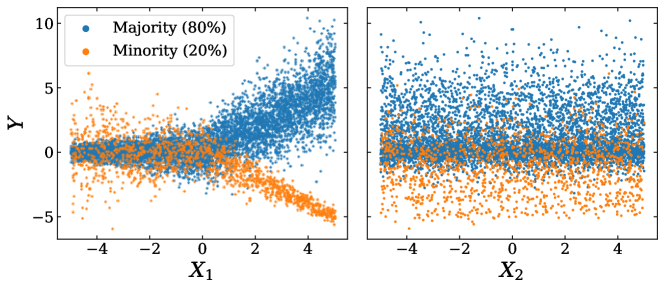
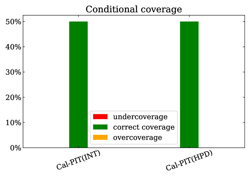
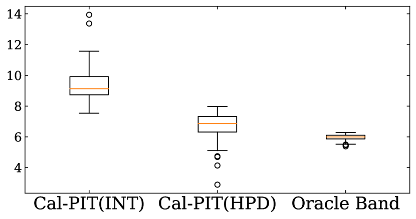
Figure 15 shows that both Cal-PIT (INT) and Cal-PIT (HPD) have set sizes that are as small as their optimal counterparts (“Oracle Band” and “Oracle HPD”, respectively), and that Cal-PIT (HPD) sets are indeed more informative (that is, the regions are smaller) than Cal-PIT (INT).

Figure 15: Average prediction set sizes for test points for different methods along with the ideal “Oracle Band” and “Oracle HPD”. Box plots show the size distribution for multiple trials of the experiment. Cal-PIT achieves prediction sets that are at least as tight as those by other methods, while simultaneously providing more accurate coverage.

We saw that this example is difficult for both quantile regression (QR) and orthogonal quantile regression (OQR) to learn (see Figure 4). OQR augments the standard pinball loss of QR with a penalty on the correlation between prediction set size and coverage, which can improve conditional coverage in certain settings (Feldman, Bates and Romano, 2021), but is not very helpful in this example. Figure 16 shows that the initial prediction sets learned by QR have bad conditional coverage, but also do not have much correlation between size and coverage. Thus, the penalty applied by OQR is unable to substantially improve upon the QR results.

Figure 16: Top: Prediction sets from quantile regression (QR). We see clear correlations between size and coverage, but note that $X_{0}$ is not actually available as a predictor, i.e. we cannot “see” the blue and orange colors. The overall correlations, without the colors, are weak. Bottom: Prediction sets from orthogonalized quantile regression (OQR). Because the overall correlation between size and coverage is weak, penalizing it does not change the results very much. In particular, we still see high correlations (and bad conditional coverage) in the minority group.

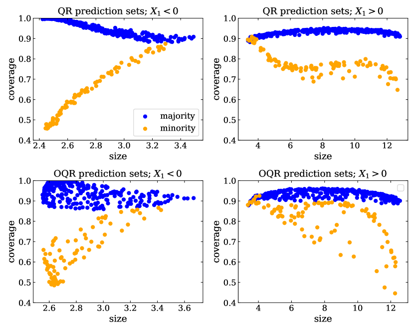
We emphasize that methods like OQR target proxies for conditional coverage, while our Cal-PIT method directly targets conditional coverage. Therefore, our method succeeds in more general settings. Example 1 is a case where penalizing the correlation between prediction set size and coverage is not a good proxy for achieving conditional coverage, so OQR is not as successful as Cal-PIT at achieving conditional coverage.

Training a regression model to learn $\widehat{r}^{\widehat{f}}(\gamma;{\mathbf{x}})$
The success of Cal-PIT depends entirely on learning an accurate representation of $\widehat{r}^{\widehat{f}}(\gamma;{\mathbf{x}})$. One can in principle choose any regression algorithm and pair it with 1. We use monotonic neural networks from Wehenkel and Louppe (2019) as our regression method as we find this architecture gives reasonably good results for all of our experiments. The network is constrained to be monotonic w.r.t. the coverage level ($\alpha$) and uses identical sets of fully connected sub-networks to learn the monotonic dependence and the unconstrained dependence separately, with the two results merged in the final layer of the network. It is known that neural networks struggle with categorical inputs and in that case, tree-based regression methods or an additional embedding step might produce better results.

For synthetic example-1 and the photometric redshift demonstration, we use a network architecture with 3 hidden layers with 512 nodes each and for synthetic example-2 we use a network architecture with 3 hidden layers with 128 nodes each (see Section Conditionally Calibrated Predictive Distributions by Probability-Probability Map: Application to Galaxy Redshift Estimation and Probabilistic Forecasting for the details on example 3). We use the reLU activation function Glorot, Bordes and Bengio (2011) for all the hidden layers and the AdamW optimizer Loshchilov and Hutter (2019) with an initial learning rate of 0.001 and weight decay parameter set to 0.01. We follow a multiplicative weight decay schedule given by the rule: $\mathrm{learning\ rate\ (epoch)}=\mathrm{initial\ learning\ rate}\times 0.95^{\mathrm{epoch}}$. Following assumption 4, we minimize the mean squared error to train the models. The data used to train the model is split into 90:10 partitions where 90% of the data is used to optimize the loss function and 10% of the data is used to calculate a validation mean squared error loss every epoch on a fixed grid of $\alpha$. To prevent our model from over-fitting we stop training once the validation loss does not decrease for 10 epochs and save the model with the best validation loss. We use a batch size of 2048 throughout and oversample our training data by a factor ($K$) of 50.

We used PyTorch Paszke et al. (2019) to create and train our neural network models and trained them on a single Nvidia A100 GPU. If a value of any hyperparameter is not explicitly mentioned here in the text, it implies that we used the default values set in PyTorch. Training times for all our experiments range from a few minutes to about an hour at maximum.

Details on Probabilistic Nowcasting Application

D.2 Tropical Cyclone Data

We fit our TC example to TC intensity and location data from NHC’s HURDAT2 best track database (Landsea and Franklin, 2013), and GOES longwave infrared imagery from NOAA’s MERGIR database (Janowiak, Joyce and Xie, 2020). HURDAT2 best tracks are provided at 6-hour time resolution, while the GOES IR imagery is available at a 30-minute×4-km resolution over both the North Atlantic (NAL) and Eastern North Pacific (ENP) basins from 2000–2020. Every thirty minutes during the lifetime of a storm, we record a $\sim$800 km×800 km “stamp” of IR imagery surrounding the TC location, showing cloud-top temperatures for the storm. Figure 9 (left) shows two such stamps.

The radial profile, defined as $T(r)=\frac{1}{2\pi}\int_{0}^{2\pi}T_{b}(r,\theta)d\theta$, captures the structure of cloud-top temperatures $T_{b}$ as a function of radius $r$ from the TC center and serves as an easily interpretable description of the depth and location of convection near the TC core (McNeely et al., 2020; Sanabia, Barrett and Fine, 2014). The radial profiles are computed at 5-km resolution from 0-400km (d = 80) (Figure 9, center). Finally, at each time t we stack the preceding 24 hours (48 profiles) into a structural trajectory, $\mathbf{S}_{<t}$, consisting of an image of the most recent 48 rows of the data. We visualize these summaries over time with Hovmöller diagrams (Hovmöller (1949); see Figure 9, right).

Figure 17 shows an example sequence of observed radial profiles every 30 minutes for a real TC, along with observed wind speed $Y$. We interpolate $Y$, which is available every 6 hours, to a 30-minute resolution.

Our goal is to create a synthetic example that has a similar dependency structure as actual TCs.

(a) Observed

(b) Reconstructed

Figure 17: Observed and reconstructed radial profiles ${\mathbf{X}}_{t}$ over time for Hurricane Teddy 2020 (left). These are recorded every 30 mins. We obtain a decent reconstruction by using the first 3 PCs. Observed wind speed values $Y_{t}$, recorded every 6 hours but interpolated on the same 30 min grid (right).

Figure 18: Top 3 PCA components, or empirical orthogonal functions (EOFs), for TC radial profiles.

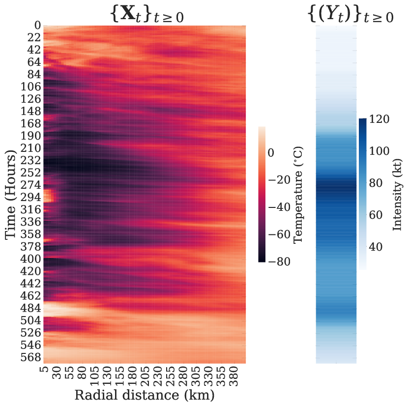
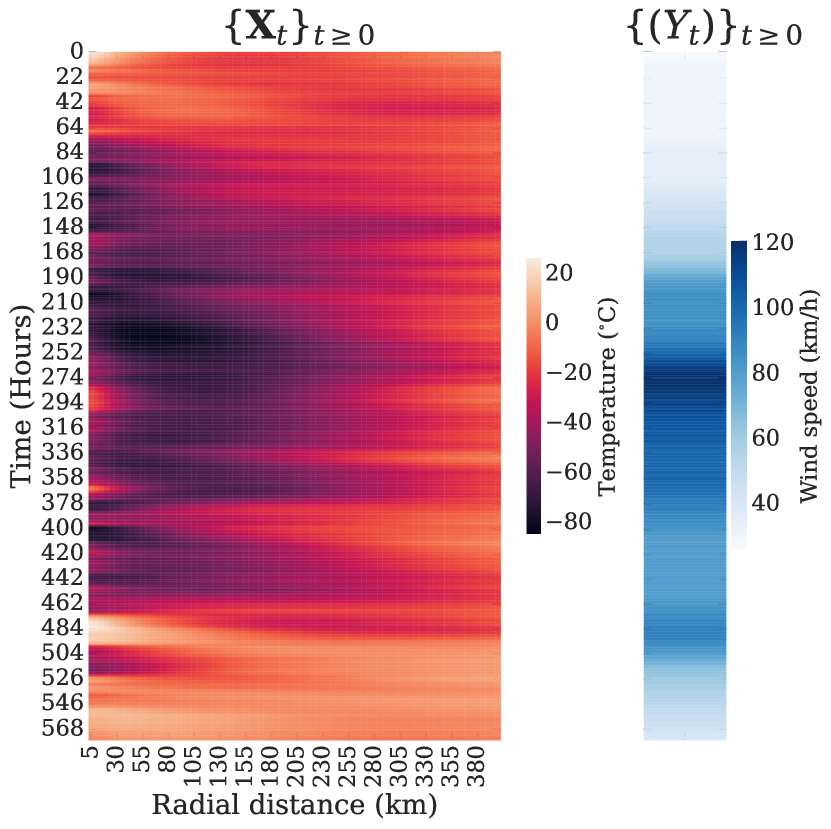
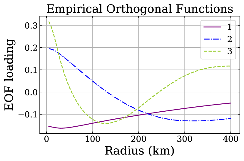
D.3 Synthetic Model for High-Dimensional Sequence Data

Using the radial profiles from all TC data, we perform a principal component analysis (PCA). Figure 18 shows the first three principal components, or empirical orthogonal functions (EOFs). Figure 17 shows the observation and reconstruction of the TC using just these three EOFs. To create the synthetic data in Example 3, we use a similar reconstruction scheme:

Let $\Delta PC_{t}:=PC_{t}-PC_{t-30m}$ be the 30-minute change in a PC coefficient at time $t$ for observed data. We fit a vector autoregression (VAR) model to $(\Delta PC1_{t},\Delta PC2_{t},\Delta PC3_{t})$ to capture the dependence of each component on its own lags as well as the lags of the other components. The model chosen by the BIC criterion has order 3, for a lag of 90 minutes.

With the fitted VAR model, we can jointly simulate synthetic time series data for $PC1,PC2,PC3$. A TC structural trajectory is constructed by multiplying simulated time series of PCA coefficients with their corresponding eigenvectors (Figure 18).

D.4 Synthetic Model for Intensities

To model the time evolution of intensities $Y$, we fit a time series regression of intensity change on its past values together with PC coefficients for present and past TC structure.

Let $Z:=\textrm{logit}(Y/200)$ so that simulated values of intensities $Y$ are reasonable, i.e. fall between 0 and 200. We then define $\Delta Z_{t}=Z_{t}-Z_{t-6h}$. Finally, we fit the following linear regression model for $\Delta Z$:

$$\Delta Z_{t}= \beta_{0}+\beta_{1}Z_{t-6h}+\beta_{2}\Delta Z_{t-6h}+\beta_{3}PC1_{t}+\beta_{4}PC2_{t}+\beta_{5}PC3_{t}$$ (15)

$$+\beta_{6}PC1_{t-6h}+\beta_{7}PC2_{t-6h}+\beta_{8}PC3_{t-6h}+\beta_{9}PC1_{t-12h}$$

$$+\beta_{10}PC2_{t-12h}+\beta_{11}PC3_{t-18h}+\beta_{12}PC2_{t-24h}+\epsilon_{t}$$

where $\epsilon_{t}$ is Gaussian noise with mean 0 and standard deviation set to the root mean squared error between the real and predicted radial profiles in the training set. Note that $\Delta Z_{t}$ has dependencies on its own lagged values as well as lagged values of $PC_{t}$.
Figure 10 in Section 5.2 shows an example TC with simulated radial profiles that update every 30 minutes, with accompanying simulated wind speed $Y$ every 30 minutes.
As a sanity check, we check that the marginal distributions of the simulated and real wind speed values ($Y$) look similar, as shown in Figure 19.

Figure 19: Left: Marginal distribution of generated wind speed values $Y$, based on the model in Equation 15. Right: Marginal distribution of observed wind speed values.

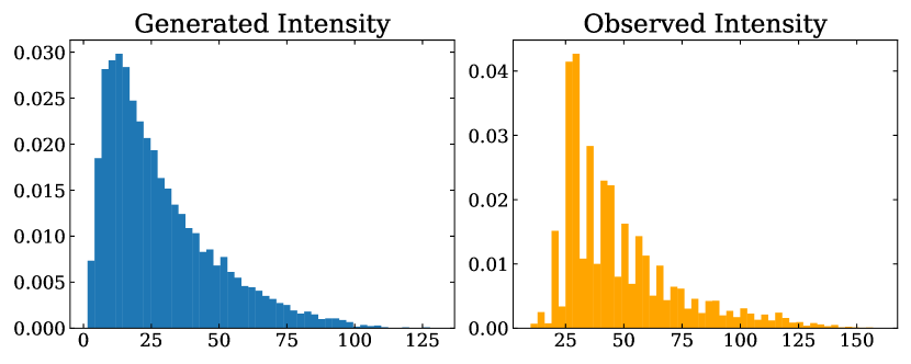
D.5 Re-calibration of Convolutional MDN Results of Intensity Distribution

With our trained VAR model, we generate a very long time series for $PC1,PC2,PC3$ with a value of the $PC$’s randomly selected from the training set of storms as the initial point. The time series is then divided into 24-hour-long chunks and the structural trajectory and intensities are reconstructed. We create 8000 such instances for our training set, 8000 more for our calibration set, and 4000 instances for our test sets. We rejected a 24-hour long window between each chunk of the time series to ensure that each instance has no memory of the previous ones.

We fit a unimodal Gaussian neural density model to estimate the conditional density $f(y|{\mathbf{s}})$ of TC intensities given past radial profiles. Specifically, we fit a convolutional mixture density network (ConvMDN, D’Isanto and Polsterer (2018)) with a single Gaussian component, two convolutional and two fully connected layers which gives an initial estimate of $f(y|{\mathbf{s}})$.

We then use a convolutional neural network LeCun et al. (1989); Fukushima and Miyake (1982) model with two convolutional layers followed by 5 fully connected layers which take the structural trajectory images and the coverage level ($\alpha$) as inputs training. The network output is restricted to be monotonic w.r.t. $\alpha$ Wehenkel and Louppe (2019). For both the models we use ReLU activations (Glorot, Bordes and Bengio, 2011) for intermediate layers and train using the Adam optimizer (Kingma and Ba, 2014) with learning rate $10^{-3}$, $\beta_{1}=0.9$, and $\beta_{2}=0.999$. We use the same multiplicative learning rate decay schedule mentioned in Conditionally Calibrated Predictive Distributions by Probability-Probability Map: Application to Galaxy Redshift Estimation and Probabilistic Forecasting.

D.6 Additional Example 3 Results

Figure 20: Oracle bands for the distribution of $Y_{t+6h}$ conditional on $\{\mathbf{S}_{<t}\}$ and $\{Y_{<t}\}$ at fixed values of $t$, for simulated TCs. The distributions show skewness, which may explain why the uncalibrated ConvMDN does not fit perfectly. Moreover, the calibrated prediction sets appear to track the observed trajectories (black curves) more closely than the ConvMDN.

Figure 21: Prediction sets for simulated TCs, before and after calibration. True trajectories are solid black, and prediction sets at test points are in blue.

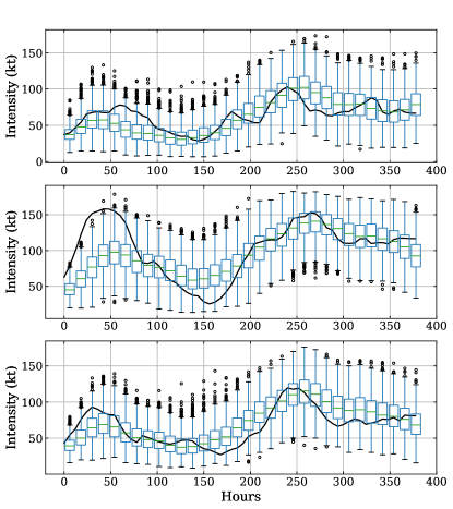
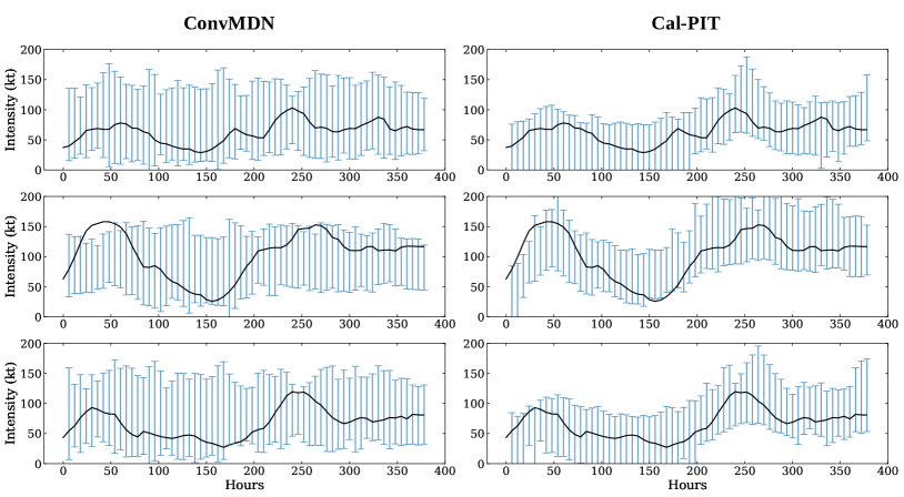
The ConvMDN struggles in this example because of the conditional distribution of $Y|\mathbf{S}$ sometimes being skewed towards larger intensities; this phenomenon can partly be observed in Figure 20, where we show the distribution of $Y_{t}$ at fixed values of $t$ for some example simulated TCs. Cal-PIT is able to adjust for the model misspecification (similar to Example 2), resulting in narrower prediction bands that are still conditionally valid. Figure 21 shows a few more examples of prediction sets for simulated TCs before and after calibration.

References

- Alkema, Raftery and Clark (2007) {barticle}[author] \bauthor\bsnmAlkema, \bfnmLeontine\binitsL., \bauthor\bsnmRaftery, \bfnmAdrian E\binitsA. E. and \bauthor\bsnmClark, \bfnmSamuel J\binitsS. J. (\byear2007). \btitleProbabilistic projections of HIV prevalence using Bayesian melding. \bjournalThe annals of applied statistics \bvolume1 \bpages229–248. \endbibitem
- Almosallam, Jarvis and Roberts (2016) {barticle}[author] \bauthor\bsnmAlmosallam, \bfnmIbrahim A.\binitsI. A., \bauthor\bsnmJarvis, \bfnmMatt J.\binitsM. J. and \bauthor\bsnmRoberts, \bfnmStephen J.\binitsS. J. (\byear2016). \btitleGPZ: non-stationary sparse Gaussian processes for heteroscedastic uncertainty estimation in photometric redshifts. \bjournalMNRAS \bvolume462 \bpages726-739. \bdoi10.1093/mnras/stw1618 \endbibitem
- Ambrogioni et al. (2017) {barticle}[author] \bauthor\bsnmAmbrogioni, \bfnmLuca\binitsL., \bauthor\bsnmGüçlü, \bfnmUmut\binitsU., \bauthor\bsnmvan Gerven, \bfnmMarcel A. J.\binitsM. A. J. and \bauthor\bsnmMaris, \bfnmEric\binitsE. (\byear2017). \btitleThe Kernel Mixture Network: A Nonparametric Method for Conditional Density Estimation of Continuous Random Variables. \bjournalarXiv e-prints \bpagesarXiv:1705.07111. \endbibitem
- Amerise (2018) {barticle}[author] \bauthor\bsnmAmerise, \bfnmIlaria Lucrezia\binitsI. L. (\byear2018). \btitleQuantile Regression Estimation Using Non-Crossing Constraints. \bjournalJournal of Mathematics and Statistics \bvolume14 \bpages107-118. \bdoi10.3844/jmssp.2018.107.118 \endbibitem
- Arnouts et al. (1999) {barticle}[author] \bauthor\bsnmArnouts, \bfnmS.\binitsS., \bauthor\bsnmCristiani, \bfnmS.\binitsS., \bauthor\bsnmMoscardini, \bfnmL.\binitsL., \bauthor\bsnmMatarrese, \bfnmS.\binitsS., \bauthor\bsnmLucchin, \bfnmF.\binitsF., \bauthor\bsnmFontana, \bfnmA.\binitsA. and \bauthor\bsnmGiallongo, \bfnmE.\binitsE. (\byear1999). \btitleMeasuring and modelling the redshift evolution of clustering: the Hubble Deep Field North. \bjournalMNRAS \bvolume310 \bpages540-556. \bdoi10.1046/j.1365-8711.1999.02978.x \endbibitem
- Barnes, Barnes and Gordillo (2021) {barticle}[author] \bauthor\bsnmBarnes, \bfnmElizabeth A\binitsE. A., \bauthor\bsnmBarnes, \bfnmRandal J\binitsR. J. and \bauthor\bsnmGordillo, \bfnmNicolas\binitsN. (\byear2021). \btitleAdding Uncertainty to Neural Network Regression Tasks in the Geosciences. \bjournalarXiv preprint arXiv:2109.07250. \endbibitem
- Beaumont, Zhang and Balding (2002) {barticle}[author] \bauthor\bsnmBeaumont, \bfnmMark A\binitsM. A., \bauthor\bsnmZhang, \bfnmWenyang\binitsW. and \bauthor\bsnmBalding, \bfnmDavid J\binitsD. J. (\byear2002). \btitleApproximate Bayesian computation in population genetics. \bjournalGenetics \bvolume162 \bpages2025–2035. \endbibitem
- Beck et al. (2016) {barticle}[author] \bauthor\bsnmBeck, \bfnmRóbert\binitsR., \bauthor\bsnmDobos, \bfnmLászló\binitsL., \bauthor\bsnmBudavári, \bfnmTamás\binitsT., \bauthor\bsnmSzalay, \bfnmAlexander S.\binitsA. S. and \bauthor\bsnmCsabai, \bfnmIstván\binitsI. (\byear2016). \btitlePhotometric redshifts for the SDSS Data Release 12. \bjournalMNRAS \bvolume460 \bpages1371-1381. \bdoi10.1093/mnras/stw1009 \endbibitem
- Benítez (2000) {barticle}[author] \bauthor\bsnmBenítez, \bfnmNarciso\binitsN. (\byear2000). \btitleBayesian Photometric Redshift Estimation. \bjournalApJ \bvolume536 \bpages571-583. \bdoi10.1086/308947 \endbibitem
- Bierens (1983) {barticle}[author] \bauthor\bsnmBierens, \bfnmHerman J\binitsH. J. (\byear1983). \btitleUniform consistency of kernel estimators of a regression function under generalized conditions. \bjournalJournal of the American Statistical Association \bvolume78 \bpages699–707. \endbibitem
- Bishop (1994) {bunpublished}[author] \bauthor\bsnmBishop, \bfnmChristopher M.\binitsC. M. (\byear1994). \btitleMixture density networks. \endbibitem
- Bordoloi, Lilly and Amara (2010) {barticle}[author] \bauthor\bsnmBordoloi, \bfnmR.\binitsR., \bauthor\bsnmLilly, \bfnmS. J.\binitsS. J. and \bauthor\bsnmAmara, \bfnmA.\binitsA. (\byear2010). \btitlePhoto-z performance for precision cosmology. \bjournalMonthly Notices of the Royal Astronomical Society \bvolume406 \bpages881-895. \endbibitem
- Brammer, van Dokkum and Coppi (2008) {barticle}[author] \bauthor\bsnmBrammer, \bfnmGabriel B.\binitsG. B., \bauthor\bsnmvan Dokkum, \bfnmPieter G.\binitsP. G. and \bauthor\bsnmCoppi, \bfnmPaolo\binitsP. (\byear2008). \btitleEAZY: A Fast, Public Photometric Redshift Code. \bjournalApJ \bvolume686 \bpages1503-1513. \bdoi10.1086/591786 \endbibitem
- Carrasco Kind and Brunner (2013) {barticle}[author] \bauthor\bsnmCarrasco Kind, \bfnmMatias\binitsM. and \bauthor\bsnmBrunner, \bfnmRobert J.\binitsR. J. (\byear2013). \btitleTPZ: photometric redshift PDFs and ancillary information by using prediction trees and random forests. \bjournalMNRAS \bvolume432 \bpages1483-1501. \bdoi10.1093/mnras/stt574 \endbibitem
- Cavuoti et al. (2017) {barticle}[author] \bauthor\bsnmCavuoti, \bfnmS.\binitsS., \bauthor\bsnmAmaro, \bfnmV.\binitsV., \bauthor\bsnmBrescia, \bfnmM.\binitsM., \bauthor\bsnmVellucci, \bfnmC.\binitsC., \bauthor\bsnmTortora, \bfnmC.\binitsC. and \bauthor\bsnmLongo, \bfnmG.\binitsG. (\byear2017). \btitleMETAPHOR: a machine-learning-based method for the probability density estimation of photometric redshifts. \bjournalMNRAS \bvolume465 \bpages1959-1973. \bdoi10.1093/mnras/stw2930 \endbibitem
- Chen and Guestrin (2016) {binproceedings}[author] \bauthor\bsnmChen, \bfnmTianqi\binitsT. and \bauthor\bsnmGuestrin, \bfnmCarlos\binitsC. (\byear2016). \btitleXGBoost: A Scalable Tree Boosting System. In \bbooktitleProceedings of the 22nd ACM SIGKDD International Conference on Knowledge Discovery and Data Mining. \bseriesKDD ’16 \bpages785–794. \bpublisherACM, \baddressNew York, NY, USA. \bdoi10.1145/2939672.2939785 \endbibitem
- Chernozhukov, Wüthrich and Zhu (2021) {barticle}[author] \bauthor\bsnmChernozhukov, \bfnmVictor\binitsV., \bauthor\bsnmWüthrich, \bfnmKaspar\binitsK. and \bauthor\bsnmZhu, \bfnmYinchu\binitsY. (\byear2021). \btitleDistributional conformal prediction. \bjournalProceedings of the National Academy of Sciences \bvolume118. \endbibitem
- Chung et al. (2021a) {binproceedings}[author] \bauthor\bsnmChung, \bfnmYoungseog\binitsY., \bauthor\bsnmNeiswanger, \bfnmWillie\binitsW., \bauthor\bsnmChar, \bfnmIan\binitsI. and \bauthor\bsnmSchneider, \bfnmJeff\binitsJ. (\byear2021a). \btitleBeyond Pinball Loss: Quantile Methods for Calibrated Uncertainty Quantification. In \bbooktitleAdvances in Neural Information Processing Systems 34: Annual Conference on Neural Information Processing Systems 2021, NeurIPS 2021, December 6-14, 2021, virtual (\beditor\bfnmMarc’Aurelio\binitsM. \bsnmRanzato, \beditor\bfnmAlina\binitsA. \bsnmBeygelzimer, \beditor\bfnmYann N.\binitsY. N. \bsnmDauphin, \beditor\bfnmPercy\binitsP. \bsnmLiang and \beditor\bfnmJennifer Wortman\binitsJ. W. \bsnmVaughan, eds.) \bpages10971–10984. \endbibitem
- Chung et al. (2021b) {binproceedings}[author] \bauthor\bsnmChung, \bfnmYoungseog\binitsY., \bauthor\bsnmNeiswanger, \bfnmWillie\binitsW., \bauthor\bsnmChar, \bfnmIan\binitsI. and \bauthor\bsnmSchneider, \bfnmJeff\binitsJ. (\byear2021b). \btitleBeyond pinball loss: Quantile methods for calibrated uncertainty quantification. In \bbooktitleAdvances in Neural Information Processing Systems \bvolume35. \bpublisherCurran Associates, Inc. \endbibitem
- The LSST Dark Energy Science Collaboration et al. (2018) {barticle}[author] \bauthor\bsnmThe LSST Dark Energy Science Collaboration, \bauthor\bsnmMandelbaum, \bfnmRachel\binitsR., \bauthor\bsnmEifler, \bfnmTim\binitsT., \bauthor\bsnmHložek, \bfnmRenée\binitsR., \bauthor\bsnmCollett, \bfnmThomas\binitsT., \bauthor\bsnmGawiser, \bfnmEric\binitsE., \bauthor\bsnmScolnic, \bfnmDaniel\binitsD., \bauthor\bsnmAlonso, \bfnmDavid\binitsD., \bauthor\bsnmAwan, \bfnmHumna\binitsH., \bauthor\bsnmBiswas, \bfnmRahul\binitsR., \bauthor\bsnmBlazek, \bfnmJonathan\binitsJ., \bauthor\bsnmBurchat, \bfnmPatricia\binitsP., \bauthor\bsnmChisari, \bfnmNora Elisa\binitsN. E., \bauthor\bsnmDell’Antonio, \bfnmIan\binitsI., \bauthor\bsnmDigel, \bfnmSeth\binitsS., \bauthor\bsnmFrieman, \bfnmJosh\binitsJ., \bauthor\bsnmGoldstein, \bfnmDaniel A.\binitsD. A., \bauthor\bsnmHook, \bfnmIsobel\binitsI., \bauthor\bsnmIvezić, \bfnmŽeljko\binitsŽ., \bauthor\bsnmKahn, \bfnmSteven M.\binitsS. M., \bauthor\bsnmKamath, \bfnmSowmya\binitsS., \bauthor\bsnmKirkby, \bfnmDavid\binitsD., \bauthor\bsnmKitching, \bfnmThomas\binitsT., \bauthor\bsnmKrause, \bfnmElisabeth\binitsE., \bauthor\bsnmLeget, \bfnmPierre-François\binitsP.-F., \bauthor\bsnmMarshall, \bfnmPhilip J.\binitsP. J., \bauthor\bsnmMeyers, \bfnmJoshua\binitsJ., \bauthor\bsnmMiyatake, \bfnmHironao\binitsH., \bauthor\bsnmNewman, \bfnmJeffrey A.\binitsJ. A., \bauthor\bsnmNichol, \bfnmRobert\binitsR., \bauthor\bsnmRykoff, \bfnmEli\binitsE., \bauthor\bsnmSanchez, \bfnmF. Javier\binitsF. J., \bauthor\bsnmSlosar, \bfnmAnže\binitsA., \bauthor\bsnmSullivan, \bfnmMark\binitsM. and \bauthor\bsnmTroxel, \bfnmM. A.\binitsM. A. (\byear2018). \btitleThe LSST Dark Energy Science Collaboration (DESC) Science Requirements Document. \bjournalarXiv e-prints \bpagesarXiv:1809.01669. \bdoi10.48550/arXiv.1809.01669 \endbibitem
- Euclid Collaboration et al. (2021) {barticle}[author] \bauthor\bsnmEuclid Collaboration, \bauthor\bsnmIlbert, \bfnmO.\binitsO., \bauthor\bsnmde la Torre, \bfnmS.\binitsS., \bauthor\bsnmMartinet, \bfnmN.\binitsN., \bauthor\bsnmWright, \bfnmA. H.\binitsA. H., \bauthor\bsnmPaltani, \bfnmS.\binitsS., \bauthor\bsnmLaigle, \bfnmC.\binitsC., \bauthor\bsnmDavidzon, \bfnmI.\binitsI., \bauthor\bsnmJullo, \bfnmE.\binitsE., \bauthor\bsnmHildebrandt, \bfnmH.\binitsH., \bauthor\bsnmMasters, \bfnmD. C.\binitsD. C., \bauthor\bsnmAmara, \bfnmA.\binitsA., \bauthor\bsnmConselice, \bfnmC. J.\binitsC. J., \bauthor\bsnmAndreon, \bfnmS.\binitsS., \bauthor\bsnmAuricchio, \bfnmN.\binitsN., \bauthor\bsnmAzzollini, \bfnmR.\binitsR., \bauthor\bsnmBaccigalupi, \bfnmC.\binitsC., \bauthor\bsnmBalaguera-Antolínez, \bfnmA.\binitsA., \bauthor\bsnmBaldi, \bfnmM.\binitsM., \bauthor\bsnmBalestra, \bfnmA.\binitsA., \bauthor\bsnmBardelli, \bfnmS.\binitsS., \bauthor\bsnmBender, \bfnmR.\binitsR., \bauthor\bsnmBiviano, \bfnmA.\binitsA., \bauthor\bsnmBodendorf, \bfnmC.\binitsC., \bauthor\bsnmBonino, \bfnmD.\binitsD., \bauthor\bsnmBorgani, \bfnmS.\binitsS., \bauthor\bsnmBoucaud, \bfnmA.\binitsA., \bauthor\bsnmBozzo, \bfnmE.\binitsE., \bauthor\bsnmBranchini, \bfnmE.\binitsE., \bauthor\bsnmBrescia, \bfnmM.\binitsM., \bauthor\bsnmBurigana, \bfnmC.\binitsC., \bauthor\bsnmCabanac, \bfnmR.\binitsR., \bauthor\bsnmCamera, \bfnmS.\binitsS., \bauthor\bsnmCapobianco, \bfnmV.\binitsV., \bauthor\bsnmCappi, \bfnmA.\binitsA., \bauthor\bsnmCarbone, \bfnmC.\binitsC., \bauthor\bsnmCarretero, \bfnmJ.\binitsJ., \bauthor\bsnmCarvalho, \bfnmC. S.\binitsC. S., \bauthor\bsnmCasas, \bfnmS.\binitsS., \bauthor\bsnmCastander, \bfnmF. J.\binitsF. J., \bauthor\bsnmCastellano, \bfnmM.\binitsM., \bauthor\bsnmCastignani, \bfnmG.\binitsG., \bauthor\bsnmCavuoti, \bfnmS.\binitsS., \bauthor\bsnmCimatti, \bfnmA.\binitsA., \bauthor\bsnmCledassou, \bfnmR.\binitsR., \bauthor\bsnmColodro-Conde, \bfnmC.\binitsC., \bauthor\bsnmCongedo, \bfnmG.\binitsG., \bauthor\bsnmConversi, \bfnmL.\binitsL., \bauthor\bsnmCopin, \bfnmY.\binitsY., \bauthor\bsnmCorcione, \bfnmL.\binitsL., \bauthor\bsnmCostille, \bfnmA.\binitsA., \bauthor\bsnmCoupon, \bfnmJ.\binitsJ., \bauthor\bsnmCourtois, \bfnmH. M.\binitsH. M., \bauthor\bsnmCropper, \bfnmM.\binitsM., \bauthor\bsnmCuby, \bfnmJ.\binitsJ., \bauthor\bsnmDa Silva, \bfnmA.\binitsA., \bauthor\bsnmDegaudenzi, \bfnmH.\binitsH., \bauthor\bsnmDi Ferdinando, \bfnmD.\binitsD., \bauthor\bsnmDubath, \bfnmF.\binitsF., \bauthor\bsnmDuncan, \bfnmC.\binitsC., \bauthor\bsnmDupac, \bfnmX.\binitsX., \bauthor\bsnmDusini, \bfnmS.\binitsS., \bauthor\bsnmEalet, \bfnmA.\binitsA., \bauthor\bsnmFabricius, \bfnmM.\binitsM., \bauthor\bsnmFarrens, \bfnmS.\binitsS., \bauthor\bsnmFerreira, \bfnmP. G.\binitsP. G., \bauthor\bsnmFinelli, \bfnmF.\binitsF., \bauthor\bsnmFosalba, \bfnmP.\binitsP., \bauthor\bsnmFotopoulou, \bfnmS.\binitsS., \bauthor\bsnmFranceschi, \bfnmE.\binitsE., \bauthor\bsnmFranzetti, \bfnmP.\binitsP., \bauthor\bsnmGaleotta, \bfnmS.\binitsS., \bauthor\bsnmGarilli, \bfnmB.\binitsB., \bauthor\bsnmGillard, \bfnmW.\binitsW., \bauthor\bsnmGillis, \bfnmB.\binitsB., \bauthor\bsnmGiocoli, \bfnmC.\binitsC., \bauthor\bsnmGozaliasl, \bfnmG.\binitsG., \bauthor\bsnmGraciá-Carpio, \bfnmJ.\binitsJ., \bauthor\bsnmGrupp, \bfnmF.\binitsF., \bauthor\bsnmGuzzo, \bfnmL.\binitsL., \bauthor\bsnmHaugan, \bfnmS. V. H.\binitsS. V. H., \bauthor\bsnmHolmes, \bfnmW.\binitsW., \bauthor\bsnmHormuth, \bfnmF.\binitsF., \bauthor\bsnmJahnke, \bfnmK.\binitsK., \bauthor\bsnmKeihanen, \bfnmE.\binitsE., \bauthor\bsnmKermiche, \bfnmS.\binitsS., \bauthor\bsnmKiessling, \bfnmA.\binitsA., \bauthor\bsnmKirkpatrick, \bfnmC. C.\binitsC. C., \bauthor\bsnmKunz, \bfnmM.\binitsM., \bauthor\bsnmKurki-Suonio, \bfnmH.\binitsH., \bauthor\bsnmLigori, \bfnmS.\binitsS., \bauthor\bsnmLilje, \bfnmP. B.\binitsP. B., \bauthor\bsnmLloro, \bfnmI.\binitsI., \bauthor\bsnmMaino, \bfnmD.\binitsD., \bauthor\bsnmMaiorano, \bfnmE.\binitsE., \bauthor\bsnmMarggraf, \bfnmO.\binitsO., \bauthor\bsnmMarkovic, \bfnmK.\binitsK., \bauthor\bsnmMarulli, \bfnmF.\binitsF., \bauthor\bsnmMassey, \bfnmR.\binitsR., \bauthor\bsnmMaturi, \bfnmM.\binitsM., \bauthor\bsnmMauri, \bfnmN.\binitsN., \bauthor\bsnmMaurogordato, \bfnmS.\binitsS., \bauthor\bsnmMcCracken, \bfnmH. J.\binitsH. J., \bauthor\bsnmMedinaceli, \bfnmE.\binitsE., \bauthor\bsnmMei, \bfnmS.\binitsS., \bauthor\bsnmMetcalf, \bfnmR. Benton\binitsR. B., \bauthor\bsnmMoresco, \bfnmM.\binitsM., \bauthor\bsnmMorin, \bfnmB.\binitsB., \bauthor\bsnmMoscardini, \bfnmL.\binitsL., \bauthor\bsnmMunari, \bfnmE.\binitsE., \bauthor\bsnmNakajima, \bfnmR.\binitsR., \bauthor\bsnmNeissner, \bfnmC.\binitsC., \bauthor\bsnmNiemi, \bfnmS.\binitsS., \bauthor\bsnmNightingale, \bfnmJ.\binitsJ., \bauthor\bsnmPadilla, \bfnmC.\binitsC., \bauthor\bsnmPasian, \bfnmF.\binitsF., \bauthor\bsnmPatrizii, \bfnmL.\binitsL., \bauthor\bsnmPedersen, \bfnmK.\binitsK., \bauthor\bsnmPello, \bfnmR.\binitsR., \bauthor\bsnmPettorino, \bfnmV.\binitsV., \bauthor\bsnmPires, \bfnmS.\binitsS., \bauthor\bsnmPolenta, \bfnmG.\binitsG., \bauthor\bsnmPoncet, \bfnmM.\binitsM., \bauthor\bsnmPopa, \bfnmL.\binitsL., \bauthor\bsnmPotter, \bfnmD.\binitsD., \bauthor\bsnmPozzetti, \bfnmL.\binitsL., \bauthor\bsnmRaison, \bfnmF.\binitsF., \bauthor\bsnmRenzi, \bfnmA.\binitsA., \bauthor\bsnmRhodes, \bfnmJ.\binitsJ., \bauthor\bsnmRiccio, \bfnmG.\binitsG., \bauthor\bsnmRomelli, \bfnmE.\binitsE., \bauthor\bsnmRoncarelli, \bfnmM.\binitsM., \bauthor\bsnmRossetti, \bfnmE.\binitsE., \bauthor\bsnmSaglia, \bfnmR.\binitsR., \bauthor\bsnmSánchez, \bfnmA. G.\binitsA. G., \bauthor\bsnmSapone, \bfnmD.\binitsD., \bauthor\bsnmSchneider, \bfnmP.\binitsP., \bauthor\bsnmSchrabback, \bfnmT.\binitsT., \bauthor\bsnmScottez, \bfnmV.\binitsV., \bauthor\bsnmSecroun, \bfnmA.\binitsA., \bauthor\bsnmSeidel, \bfnmG.\binitsG., \bauthor\bsnmSerrano, \bfnmS.\binitsS., \bauthor\bsnmSirignano, \bfnmC.\binitsC., \bauthor\bsnmSirri, \bfnmG.\binitsG., \bauthor\bsnmStanco, \bfnmL.\binitsL., \bauthor\bsnmSureau, \bfnmF.\binitsF., \bauthor\bsnmTallada Crespá, \bfnmP.\binitsP., \bauthor\bsnmTenti, \bfnmM.\binitsM., \bauthor\bsnmTeplitz, \bfnmH. I.\binitsH. I., \bauthor\bsnmTereno, \bfnmI.\binitsI., \bauthor\bsnmToledo-Moreo, \bfnmR.\binitsR., \bauthor\bsnmTorradeflot, \bfnmF.\binitsF., \bauthor\bsnmTramacere, \bfnmA.\binitsA., \bauthor\bsnmValentijn, \bfnmE. A.\binitsE. A., \bauthor\bsnmValenziano, \bfnmL.\binitsL., \bauthor\bsnmValiviita, \bfnmJ.\binitsJ., \bauthor\bsnmVassallo, \bfnmT.\binitsT., \bauthor\bsnmWang, \bfnmY.\binitsY., \bauthor\bsnmWelikala, \bfnmN.\binitsN., \bauthor\bsnmWeller, \bfnmJ.\binitsJ., \bauthor\bsnmWhittaker, \bfnmL.\binitsL., \bauthor\bsnmZacchei, \bfnmA.\binitsA., \bauthor\bsnmZamorani, \bfnmG.\binitsG., \bauthor\bsnmZoubian, \bfnmJ.\binitsJ. and \bauthor\bsnmZucca, \bfnmE.\binitsE. (\byear2021). \btitleEuclid preparation. XI. Mean redshift determination from galaxy redshift probabilities for cosmic shear tomography. \bjournalA&A \bvolume647 \bpagesA117. \bdoi10.1051/0004-6361/202040237 \endbibitem
- Cook, Gelman and Rubin (2006) {barticle}[author] \bauthor\bsnmCook, \bfnmSamantha R.\binitsS. R., \bauthor\bsnmGelman, \bfnmAndrew\binitsA. and \bauthor\bsnmRubin, \bfnmDonald B.\binitsD. B. (\byear2006). \btitleValidation of software for Bayesian models using posterior quantiles. \bjournalJournal of Computational and Graphical Statistics \bvolume15 \bpages675-692. \endbibitem
- Cranmer, Brehmer and Louppe (2020) {barticle}[author] \bauthor\bsnmCranmer, \bfnmKyle\binitsK., \bauthor\bsnmBrehmer, \bfnmJohann\binitsJ. and \bauthor\bsnmLouppe, \bfnmGilles\binitsG. (\byear2020). \btitleThe frontier of simulation-based inference. \bjournalProceedings of the National Academy of Sciences \bvolume117 \bpages30055-30062. \endbibitem
- Crenshaw, Yan and vladislav doster (2023) {bmisc}[author] \bauthor\bsnmCrenshaw, \bfnmJohn Franklin\binitsJ. F., \bauthor\bsnmYan, \bfnmZi’ang\binitsZ. and \bauthor\bparticlevladislav \bsnmdoster (\byear2023). \btitlejfcrenshaw/pzflow: v3.1.1. \bdoi10.5281/zenodo.7843901 \endbibitem
- Dalmasso et al. (2020a) {barticle}[author] \bauthor\bsnmDalmasso, \bfnmN.\binitsN., \bauthor\bsnmPospisil, \bfnmT.\binitsT., \bauthor\bsnmLee, \bfnmA. B.\binitsA. B., \bauthor\bsnmIzbicki, \bfnmR.\binitsR., \bauthor\bsnmFreeman, \bfnmP. E.\binitsP. E. and \bauthor\bsnmMalz, \bfnmA. I.\binitsA. I. (\byear2020a). \btitleConditional density estimation tools in python and R with applications to photometric redshifts and likelihood-free cosmological inference. \bjournalAstronomy and Computing \bvolume30 \bpages100362. \bdoi10.1016/j.ascom.2019.100362 \endbibitem
- Dalmasso et al. (2020b) {barticle}[author] \bauthor\bsnmDalmasso, \bfnmN.\binitsN., \bauthor\bsnmPospisil, \bfnmT.\binitsT., \bauthor\bsnmLee, \bfnmA. B.\binitsA. B., \bauthor\bsnmIzbicki, \bfnmR.\binitsR., \bauthor\bsnmFreeman, \bfnmP. E.\binitsP. E. and \bauthor\bsnmMalz, \bfnmA. I.\binitsA. I. (\byear2020b). \btitleConditional density estimation tools in python and R with applications to photometric redshifts and likelihood-free cosmological inference. \bjournalAstronomy and Computing \bvolume30 \bpages100362. \bdoi10.1016/j.ascom.2019.100362 \endbibitem
- Dalmasso et al. (2021) {barticle}[author] \bauthor\bsnmDalmasso, \bfnmNiccolo\binitsN., \bauthor\bsnmMasserano, \bfnmLuca\binitsL., \bauthor\bsnmZhao, \bfnmDavid\binitsD., \bauthor\bsnmIzbicki, \bfnmRafael\binitsR. and \bauthor\bsnmLee, \bfnmAnn B\binitsA. B. (\byear2021). \btitleLikelihood-Free Frequentist Inference: Confidence Sets with Correct Conditional Coverage. \bjournalarXiv preprint arXiv:2107.03920. \endbibitem
- DeMaria et al. (2014) {barticle}[author] \bauthor\bsnmDeMaria, \bfnmMark\binitsM., \bauthor\bsnmSampson, \bfnmCharles R.\binitsC. R., \bauthor\bsnmKnaff, \bfnmJohn A.\binitsJ. A. and \bauthor\bsnmMusgrave, \bfnmKate D.\binitsK. D. (\byear2014). \btitleIs Tropical Cyclone Intensity Guidance Improving? \bjournalBulletin of the American Meteorological Society \bvolume95 \bpages387-398. \bdoi10.1175/BAMS-D-12-00240.1 \endbibitem
- Dey et al. (2021) {barticle}[author] \bauthor\bsnmDey, \bfnmBiprateep\binitsB., \bauthor\bsnmAndrews, \bfnmBrett H.\binitsB. H., \bauthor\bsnmNewman, \bfnmJeffrey A.\binitsJ. A., \bauthor\bsnmMao, \bfnmYao-Yuan\binitsY.-Y., \bauthor\bsnmRau, \bfnmMarkus Michael\binitsM. M. and \bauthor\bsnmZhou, \bfnmRongpu\binitsR. (\byear2021). \btitlePhotometric Redshifts from SDSS Images with an Interpretable Deep Capsule Network. \bjournalarXiv e-prints \bpagesarXiv:2112.03939. \endbibitem
- Dhariwal and Nichol (2021) {binproceedings}[author] \bauthor\bsnmDhariwal, \bfnmPrafulla\binitsP. and \bauthor\bsnmNichol, \bfnmAlexander Quinn\binitsA. Q. (\byear2021). \btitleDiffusion Models Beat GANs on Image Synthesis. In \bbooktitleAdvances in Neural Information Processing Systems 34: Annual Conference on Neural Information Processing Systems 2021, NeurIPS 2021, December 6-14, 2021, virtual (\beditor\bfnmMarc’Aurelio\binitsM. \bsnmRanzato, \beditor\bfnmAlina\binitsA. \bsnmBeygelzimer, \beditor\bfnmYann N.\binitsY. N. \bsnmDauphin, \beditor\bfnmPercy\binitsP. \bsnmLiang and \beditor\bfnmJennifer Wortman\binitsJ. W. \bsnmVaughan, eds.) \bpages8780–8794. \endbibitem
- Dinh, Krueger and Bengio (2014) {barticle}[author] \bauthor\bsnmDinh, \bfnmLaurent\binitsL., \bauthor\bsnmKrueger, \bfnmDavid\binitsD. and \bauthor\bsnmBengio, \bfnmYoshua\binitsY. (\byear2014). \btitleNICE: Non-linear Independent Components Estimation. \bjournalarXiv e-prints \bpagesarXiv:1410.8516. \bdoi10.48550/arXiv.1410.8516 \endbibitem
- Dinh, Sohl-Dickstein and Bengio (2016) {barticle}[author] \bauthor\bsnmDinh, \bfnmLaurent\binitsL., \bauthor\bsnmSohl-Dickstein, \bfnmJascha\binitsJ. and \bauthor\bsnmBengio, \bfnmSamy\binitsS. (\byear2016). \btitleDensity estimation using Real NVP. \bjournalarXiv e-prints \bpagesarXiv:1605.08803. \bdoi10.48550/arXiv.1605.08803 \endbibitem
- Durkan et al. (2019) {barticle}[author] \bauthor\bsnmDurkan, \bfnmConor\binitsC., \bauthor\bsnmBekasov, \bfnmArtur\binitsA., \bauthor\bsnmMurray, \bfnmIain\binitsI. and \bauthor\bsnmPapamakarios, \bfnmGeorge\binitsG. (\byear2019). \btitleNeural Spline Flows. \bjournalarXiv e-prints \bpagesarXiv:1906.04032. \bdoi10.48550/arXiv.1906.04032 \endbibitem
- Dutordoir et al. (2018) {binproceedings}[author] \bauthor\bsnmDutordoir, \bfnmVincent\binitsV., \bauthor\bsnmSalimbeni, \bfnmHugh\binitsH., \bauthor\bsnmHensman, \bfnmJames\binitsJ. and \bauthor\bsnmDeisenroth, \bfnmMarc Peter\binitsM. P. (\byear2018). \btitleGaussian Process Conditional Density Estimation. In \bbooktitleAdvances in Neural Information Processing Systems 31: Annual Conference on Neural Information Processing Systems 2018, NeurIPS 2018, December 3-8, 2018, Montréal, Canada (\beditor\bfnmSamy\binitsS. \bsnmBengio, \beditor\bfnmHanna M.\binitsH. M. \bsnmWallach, \beditor\bfnmHugo\binitsH. \bsnmLarochelle, \beditor\bfnmKristen\binitsK. \bsnmGrauman, \beditor\bfnmNicolò\binitsN. \bsnmCesa-Bianchi and \beditor\bfnmRoman\binitsR. \bsnmGarnett, eds.) \bpages2391–2401. \endbibitem
- D’Isanto and Polsterer (2018) {barticle}[author] \bauthor\bsnmD’Isanto, \bfnmAntonio\binitsA. and \bauthor\bsnmPolsterer, \bfnmKai Lars\binitsK. L. (\byear2018). \btitlePhotometric redshift estimation via deep learning. Generalized and pre-classification-less, image based, fully probabilistic redshifts. \bjournalAstronomy & Astrophysics \bvolume609 \bpagesA111. \endbibitem
- Fasiolo et al. (2021) {barticle}[author] \bauthor\bsnmFasiolo, \bfnmMatteo\binitsM., \bauthor\bsnmWood, \bfnmSimon N.\binitsS. N., \bauthor\bsnmZaffran, \bfnmMargaux\binitsM., \bauthor\bsnmNedellec, \bfnmRaphaël\binitsR. and \bauthor\bsnmGoude, \bfnmYannig\binitsY. (\byear2021). \btitleFast Calibrated Additive Quantile Regression. \bjournalJournal of the American Statistical Association \bvolume116 \bpages1402-1412. \bdoi10.1080/01621459.2020.1725521 \endbibitem
- Feldman, Bates and Romano (2021) {barticle}[author] \bauthor\bsnmFeldman, \bfnmShai\binitsS., \bauthor\bsnmBates, \bfnmStephen\binitsS. and \bauthor\bsnmRomano, \bfnmYaniv\binitsY. (\byear2021). \btitleImproving Conditional Coverage via Orthogonal Quantile Regression. \bjournalarXiv \bpages1–20. \endbibitem
- Freeman, Izbicki and Lee (2017) {barticle}[author] \bauthor\bsnmFreeman, \bfnmPeter\binitsP., \bauthor\bsnmIzbicki, \bfnmRafael\binitsR. and \bauthor\bsnmLee, \bfnmAnn B.\binitsA. B. (\byear2017). \btitleA unified framework for constructing, tuning and assessing photometric redshift density estimates in a selection bias setting. \bjournalMonthly Notices of the Royal Astronomical Society \bvolume468 \bpages4556-4565. \bdoi10.1093/mnras/stx764 \endbibitem
- Fukushima and Miyake (1982) {barticle}[author] \bauthor\bsnmFukushima, \bfnmKunihiko\binitsK. and \bauthor\bsnmMiyake, \bfnmSei\binitsS. (\byear1982). \btitleNeocognitron: A new algorithm for pattern recognition tolerant of deformations and shifts in position. \bjournalPattern Recognition \bvolume15 \bpages455-469. \bdoihttps://doi.org/10.1016/0031-3203(82)90024-3 \endbibitem
- Gal and Ghahramani (2016) {binproceedings}[author] \bauthor\bsnmGal, \bfnmYarin\binitsY. and \bauthor\bsnmGhahramani, \bfnmZoubin\binitsZ. (\byear2016). \btitleDropout as a bayesian approximation: Representing model uncertainty in deep learning. In \bbooktitleInternational Conference on Machine Learning. \bseriesProceedings of Machine Learning Research \bpages1050-1059. \bpublisherPMLR. \endbibitem
- Gan and Koehler (1990) {barticle}[author] \bauthor\bsnmGan, \bfnmF. F.\binitsF. F. and \bauthor\bsnmKoehler, \bfnmK. J.\binitsK. J. (\byear1990). \btitleGoodness-of-Fit Tests Based on P-P Probability Plots. \bjournalTechnometrics \bvolume32 \bpages289-303. \bdoi10.1080/00401706.1990.10484682 \endbibitem
- Girard, Guillou and Stupfler (2014) {barticle}[author] \bauthor\bsnmGirard, \bfnmStéphane\binitsS., \bauthor\bsnmGuillou, \bfnmArmelle\binitsA. and \bauthor\bsnmStupfler, \bfnmGilles\binitsG. (\byear2014). \btitleUniform strong consistency of a frontier estimator using kernel regression on high order moments. \bjournalESAIM: Probability and Statistics \bvolume18 \bpages642–666. \endbibitem
- Glorot, Bordes and Bengio (2011) {binproceedings}[author] \bauthor\bsnmGlorot, \bfnmXavier\binitsX., \bauthor\bsnmBordes, \bfnmAntoine\binitsA. and \bauthor\bsnmBengio, \bfnmYoshua\binitsY. (\byear2011). \btitleDeep Sparse Rectifier Neural Networks. In \bbooktitleProceedings of the Fourteenth International Conference on Artificial Intelligence and Statistics (\beditor\bfnmGeoffrey\binitsG. \bsnmGordon, \beditor\bfnmDavid\binitsD. \bsnmDunson and \beditor\bfnmMiroslav\binitsM. \bsnmDudík, eds.). \bseriesProceedings of Machine Learning Research \bvolume15 \bpages315–323. \bpublisherJMLR Workshop and Conference Proceedings, \baddressFort Lauderdale, FL, USA. \endbibitem
- Gneiting (2008) {barticle}[author] \bauthor\bsnmGneiting, \bfnmTilmann\binitsT. (\byear2008). \btitleProbabilistic forecasting. \bjournalJournal of the Royal Statistical Society. Series A (Statistics in Society) \bpages319–321. \endbibitem
- Gneiting and Katzfuss (2014) {barticle}[author] \bauthor\bsnmGneiting, \bfnmTilmann\binitsT. and \bauthor\bsnmKatzfuss, \bfnmMatthias\binitsM. (\byear2014). \btitleProbabilistic Forecasting. \bjournalAnnual Review of Statistics and Its Application \bvolume1 \bpages125-151. \bdoi10.1146/annurev-statistics-062713-085831 \endbibitem
- Goan and Fookes (2020) {barticle}[author] \bauthor\bsnmGoan, \bfnmEthan\binitsE. and \bauthor\bsnmFookes, \bfnmClinton\binitsC. (\byear2020). \btitleBayesian Neural Networks: An Introduction and Survey. \bjournalCoRR \bvolumeabs/2006.12024. \endbibitem
- Graff et al. (2014) {barticle}[author] \bauthor\bsnmGraff, \bfnmPhilip\binitsP., \bauthor\bsnmFeroz, \bfnmFarhan\binitsF., \bauthor\bsnmHobson, \bfnmMichael P.\binitsM. P. and \bauthor\bsnmLasenby, \bfnmAnthony\binitsA. (\byear2014). \btitleSKYNET: an efficient and robust neural network training tool for machine learning in astronomy. \bjournalMNRAS \bvolume441 \bpages1741-1759. \bdoi10.1093/mnras/stu642 \endbibitem
- Graham et al. (2018) {barticle}[author] \bauthor\bsnmGraham, \bfnmMelissa L.\binitsM. L., \bauthor\bsnmConnolly, \bfnmAndrew J.\binitsA. J., \bauthor\bsnmIvezić, \bfnmŽeljko\binitsŽ., \bauthor\bsnmSchmidt, \bfnmSamuel J.\binitsS. J., \bauthor\bsnmJones, \bfnmR. Lynne\binitsR. L., \bauthor\bsnmJurić, \bfnmMario\binitsM., \bauthor\bsnmDaniel, \bfnmScott F.\binitsS. F. and \bauthor\bsnmYoachim, \bfnmPeter\binitsP. (\byear2018). \btitlePhotometric Redshifts with the LSST: Evaluating Survey Observing Strategies. \bjournalAJ \bvolume155 \bpages1. \bdoi10.3847/1538-3881/aa99d4 \endbibitem
- Greenberg, Nonnenmacher and Macke (2019) {binproceedings}[author] \bauthor\bsnmGreenberg, \bfnmDavid\binitsD., \bauthor\bsnmNonnenmacher, \bfnmMarcel\binitsM. and \bauthor\bsnmMacke, \bfnmJakob\binitsJ. (\byear2019). \btitleAutomatic posterior transformation for likelihood-free inference. In \bbooktitleInternational Conference on Machine Learning \bpages2404–2414. \bpublisherPMLR. \endbibitem
- Griffin, Wimmers and Velden (2022) {barticle}[author] \bauthor\bsnmGriffin, \bfnmSarah M\binitsS. M., \bauthor\bsnmWimmers, \bfnmAnthony\binitsA. and \bauthor\bsnmVelden, \bfnmChristopher S\binitsC. S. (\byear2022). \btitlePredicting Rapid Intensification in North Atlantic and Eastern North Pacific Tropical Cyclones using a Convolutional Neural Network. \bjournalWeather and Forecasting. \endbibitem
- Guo et al. (2017) {binproceedings}[author] \bauthor\bsnmGuo, \bfnmChuan\binitsC., \bauthor\bsnmPleiss, \bfnmGeoff\binitsG., \bauthor\bsnmSun, \bfnmYu\binitsY. and \bauthor\bsnmWeinberger, \bfnmKilian Q.\binitsK. Q. (\byear2017). \btitleOn Calibration of Modern Neural Networks. In \bbooktitleProceedings of the 34th International Conference on Machine Learning (\beditor\bfnmDoina\binitsD. \bsnmPrecup and \beditor\bfnmYee Whye\binitsY. W. \bsnmTeh, eds.). \bseriesProceedings of Machine Learning Research \bvolume70 \bpages1321–1330. \bpublisherPMLR. \endbibitem
- Györfi et al. (2002) {bbook}[author] \bauthor\bsnmGyörfi, \bfnmLászló\binitsL., \bauthor\bsnmKohler, \bfnmMichael\binitsM., \bauthor\bsnmKrzyzak, \bfnmAdam\binitsA., \bauthor\bsnmWalk, \bfnmHarro\binitsH. \betalet al. (\byear2002). \btitleA distribution-free theory of nonparametric regression \bvolume1. \bpublisherSpringer. \endbibitem
- Hardle et al. (1984) {barticle}[author] \bauthor\bsnmHardle, \bfnmW\binitsW., \bauthor\bsnmLuckhaus, \bfnmStephan\binitsS. \betalet al. (\byear1984). \btitleUniform consistency of a class of regression function estimators. \bjournalThe Annals of Statistics \bvolume12 \bpages612–623. \endbibitem
- Ho, Jain and Abbeel (2020) {barticle}[author] \bauthor\bsnmHo, \bfnmJonathan\binitsJ., \bauthor\bsnmJain, \bfnmAjay\binitsA. and \bauthor\bsnmAbbeel, \bfnmPieter\binitsP. (\byear2020). \btitleDenoising Diffusion Probabilistic Models. \bjournalCoRR \bvolumeabs/2006.11239. \endbibitem
- Ho and Salimans (2022) {barticle}[author] \bauthor\bsnmHo, \bfnmJonathan\binitsJ. and \bauthor\bsnmSalimans, \bfnmTim\binitsT. (\byear2022). \btitleClassifier-Free Diffusion Guidance. \bjournalCoRR \bvolumeabs/2207.12598. \bdoi10.48550/arXiv.2207.12598 \endbibitem
- Hovmöller (1949) {barticle}[author] \bauthor\bsnmHovmöller, \bfnmErnest\binitsE. (\byear1949). \btitleThe trough-and-ridge diagram. \bjournalTellus \bvolume1 \bpages62-66. \endbibitem
- Izbicki and Lee (2016) {barticle}[author] \bauthor\bsnmIzbicki, \bfnmRafael\binitsR. and \bauthor\bsnmLee, \bfnmAnn B\binitsA. B. (\byear2016). \btitleNonparametric conditional density estimation in a high-dimensional regression setting. \bjournalJournal of Computational and Graphical Statistics \bvolume25 \bpages1297–1316. \endbibitem
- Izbicki and Lee (2017) {barticle}[author] \bauthor\bsnmIzbicki, \bfnmRafael\binitsR. and \bauthor\bsnmLee, \bfnmAnn B\binitsA. B. (\byear2017). \btitleConverting high-dimensional regression to high-dimensional conditional density estimation. \bjournalElectronic Journal of Statistics \bvolume11 \bpages2800–2831. \endbibitem
- Izbicki, Lee and Pospisil (2019) {barticle}[author] \bauthor\bsnmIzbicki, \bfnmRafael\binitsR., \bauthor\bsnmLee, \bfnmAnn B.\binitsA. B. and \bauthor\bsnmPospisil, \bfnmTaylor\binitsT. (\byear2019). \btitleABC–CDE: Toward Approximate Bayesian Computation With Complex High-Dimensional Data and Limited Simulations. \bjournalJournal of Computational and Graphical Statistics \bpages1–20. \bdoi10.1080/10618600.2018.1546594 \endbibitem
- Izbicki, Shimizu and Stern (2020) {binproceedings}[author] \bauthor\bsnmIzbicki, \bfnmRafael\binitsR., \bauthor\bsnmShimizu, \bfnmGilson\binitsG. and \bauthor\bsnmStern, \bfnmRafael\binitsR. (\byear2020). \btitleFlexible distribution-free conditional predictive bands using density estimators. In \bbooktitleInternational Conference on Artificial Intelligence and Statistics \bpages3068–3077. \bpublisherPMLR. \endbibitem
- Izbicki, Shimizu and Stern (2022) {barticle}[author] \bauthor\bsnmIzbicki, \bfnmRafael\binitsR., \bauthor\bsnmShimizu, \bfnmGilson\binitsG. and \bauthor\bsnmStern, \bfnmRafael B.\binitsR. B. (\byear2022). \btitleCD-split and HPD-split: Efficient Conformal Regions in High Dimensions. \bjournalJournal of Machine Learning Research \bvolume23 \bpages1-32. \endbibitem
- Janowiak, Joyce and Xie (2020) {bmisc}[author] \bauthor\bsnmJanowiak, \bfnmJohn\binitsJ., \bauthor\bsnmJoyce, \bfnmBob\binitsB. and \bauthor\bsnmXie, \bfnmPingping\binitsP. (\byear2020). \btitleNCEP/CPC L3 half hourly 4km global (60S - 60N) merged IR v1. \endbibitem
- Jitkrittum, Kanagawa and Schölkopf (2020a) {binproceedings}[author] \bauthor\bsnmJitkrittum, \bfnmWittawat\binitsW., \bauthor\bsnmKanagawa, \bfnmHeishiro\binitsH. and \bauthor\bsnmSchölkopf, \bfnmBernhard\binitsB. (\byear2020a). \btitleTesting Goodness of Fit of Conditional Density Models with Kernels. In \bbooktitleProceedings of the Thirty-Sixth Conference on Uncertainty in Artificial Intelligence, UAI 2020, virtual online, August 3-6, 2020 (\beditor\bfnmRyan P.\binitsR. P. \bsnmAdams and \beditor\bfnmVibhav\binitsV. \bsnmGogate, eds.). \bseriesProceedings of Machine Learning Research \bvolume124 \bpages221–230. \bpublisherAUAI Press. \endbibitem
- Jitkrittum, Kanagawa and Schölkopf (2020b) {binproceedings}[author] \bauthor\bsnmJitkrittum, \bfnmWittawat\binitsW., \bauthor\bsnmKanagawa, \bfnmHeishiro\binitsH. and \bauthor\bsnmSchölkopf, \bfnmBernhard\binitsB. (\byear2020b). \btitleTesting Goodness of Fit of Conditional Density Models with Kernels. In \bbooktitleProceedings of the 36th Conference on Uncertainty in Artificial Intelligence (UAI) (\beditor\bfnmJonas\binitsJ. \bsnmPeters and \beditor\bfnmDavid\binitsD. \bsnmSontag, eds.). \bseriesProceedings of Machine Learning Research \bvolume124 \bpages221–230. \bpublisherPMLR. \endbibitem
- Jones and Pewsey (2009) {barticle}[author] \bauthor\bsnmJones, \bfnmM Chris\binitsM. C. and \bauthor\bsnmPewsey, \bfnmArthur\binitsA. (\byear2009). \btitleSinh-arcsinh distributions. \bjournalBiometrika \bvolume96 \bpages761–780. \endbibitem
- Jones and Pewsey (2019) {bmisc}[author] \bauthor\bsnmJones, \bfnmChris\binitsC. and \bauthor\bsnmPewsey, \bfnmArthur\binitsA. (\byear2019). \btitleThe sinh-arcsinh normal distribution. \endbibitem
- Kingma and Ba (2014) {barticle}[author] \bauthor\bsnmKingma, \bfnmDiederik P.\binitsD. P. and \bauthor\bsnmBa, \bfnmJimmy\binitsJ. (\byear2014). \btitleAdam: A method for stochastic optimization. \bjournalarXiv preprint arXiv:1412.6980. \endbibitem
- Kingma and Welling (2013) {barticle}[author] \bauthor\bsnmKingma, \bfnmDiederik P\binitsD. P. and \bauthor\bsnmWelling, \bfnmMax\binitsM. (\byear2013). \btitleAuto-Encoding Variational Bayes. \bjournalarXiv e-prints \bpagesarXiv:1312.6114. \bdoi10.48550/arXiv.1312.6114 \endbibitem
- Kleinberg, Mullainathan and Raghavan (2016) {barticle}[author] \bauthor\bsnmKleinberg, \bfnmJon\binitsJ., \bauthor\bsnmMullainathan, \bfnmSendhil\binitsS. and \bauthor\bsnmRaghavan, \bfnmManish\binitsM. (\byear2016). \btitleInherent trade-offs in the fair determination of risk scores. \bjournalarXiv preprint arXiv:1609.05807. \endbibitem
- Kobyzev, Prince and Brubaker (2021) {barticle}[author] \bauthor\bsnmKobyzev, \bfnmIvan\binitsI., \bauthor\bsnmPrince, \bfnmSimon J. D.\binitsS. J. D. and \bauthor\bsnmBrubaker, \bfnmMarcus A.\binitsM. A. (\byear2021). \btitleNormalizing Flows: An Introduction and Review of Current Methods. \bjournalIEEE Trans. Pattern Anal. Mach. Intell. \bvolume43 \bpages3964–3979. \bdoi10.1109/TPAMI.2020.2992934 \endbibitem
- Koenker and Bassett Jr. (1978) {barticle}[author] \bauthor\bsnmKoenker, \bfnmRoger\binitsR. and \bauthor\bsnmBassett Jr., \bfnmGilbert\binitsG. (\byear1978). \btitleRegression quantiles. \bjournalEconometrica: Journal of the Econometric Society \bpages33–50. \endbibitem
- Koenker and Hallock (2001) {barticle}[author] \bauthor\bsnmKoenker, \bfnmRoger\binitsR. and \bauthor\bsnmHallock, \bfnmKevin F.\binitsK. F. (\byear2001). \btitleQuantile regression. \bjournalJournal of Economic Perspectives \bvolume15 \bpages143–156. \endbibitem
- Kolouri et al. (2017) {barticle}[author] \bauthor\bsnmKolouri, \bfnmSoheil\binitsS., \bauthor\bsnmPark, \bfnmSe Rim\binitsS. R., \bauthor\bsnmThorpe, \bfnmMatthew\binitsM., \bauthor\bsnmSlepcev, \bfnmDejan\binitsD. and \bauthor\bsnmRohde, \bfnmGustavo K\binitsG. K. (\byear2017). \btitleOptimal mass transport: Signal processing and machine-learning applications. \bjournalIEEE signal processing magazine \bvolume34 \bpages43–59. \endbibitem
- Kuleshov, Fenner and Ermon (2018) {binproceedings}[author] \bauthor\bsnmKuleshov, \bfnmVolodymyr\binitsV., \bauthor\bsnmFenner, \bfnmNathan\binitsN. and \bauthor\bsnmErmon, \bfnmStefano\binitsS. (\byear2018). \btitleAccurate uncertainties for deep learning using calibrated regression. In \bbooktitleInternational conference on machine learning \bpages2796–2804. \bpublisherPMLR. \endbibitem
- Kull et al. (2019) {barticle}[author] \bauthor\bsnmKull, \bfnmMeelis\binitsM., \bauthor\bsnmPerelló-Nieto, \bfnmMiquel\binitsM., \bauthor\bsnmKängsepp, \bfnmMarkus\binitsM., \bauthor\bparticlede Menezes e \bsnmSilva Filho, \bfnmTelmo\binitsT., \bauthor\bsnmSong, \bfnmHao\binitsH. and \bauthor\bsnmFlach, \bfnmPeter A.\binitsP. A. (\byear2019). \btitleBeyond temperature scaling: Obtaining well-calibrated multiclass probabilities with Dirichlet calibration. \bjournalCoRR \bvolumeabs/1910.12656. \endbibitem
- Lakshminarayanan, Pritzel and Blundell (2017) {barticle}[author] \bauthor\bsnmLakshminarayanan, \bfnmBalaji\binitsB., \bauthor\bsnmPritzel, \bfnmAlexander\binitsA. and \bauthor\bsnmBlundell, \bfnmCharles\binitsC. (\byear2017). \btitleSimple and scalable predictive uncertainty estimation using deep ensembles. \bjournalAdvances in neural information processing systems \bvolume30. \endbibitem
- Landsea and Franklin (2013) {barticle}[author] \bauthor\bsnmLandsea, \bfnmChristopher W.\binitsC. W. and \bauthor\bsnmFranklin, \bfnmJames L.\binitsJ. L. (\byear2013). \btitleAtlantic hurricane database uncertainty and presentation of a new database format. \bjournalMonthly Weather Review \bvolume141 \bpages3576-3592. \endbibitem
- LeCun et al. (1989) {barticle}[author] \bauthor\bsnmLeCun, \bfnmYann\binitsY., \bauthor\bsnmBoser, \bfnmBernhard E.\binitsB. E., \bauthor\bsnmDenker, \bfnmJohn S.\binitsJ. S., \bauthor\bsnmHenderson, \bfnmDonnie\binitsD., \bauthor\bsnmHoward, \bfnmRichard E.\binitsR. E., \bauthor\bsnmHubbard, \bfnmWayne E.\binitsW. E. and \bauthor\bsnmJackel, \bfnmLawrence D.\binitsL. D. (\byear1989). \btitleBackpropagation Applied to Handwritten Zip Code Recognition. \bjournalNeural Comput. \bvolume1 \bpages541–551. \bdoi10.1162/neco.1989.1.4.541 \endbibitem
- Lei et al. (2018) {barticle}[author] \bauthor\bsnmLei, \bfnmJing\binitsJ., \bauthor\bsnmG’Sell, \bfnmMax\binitsM., \bauthor\bsnmRinaldo, \bfnmAlessandro\binitsA., \bauthor\bsnmTibshirani, \bfnmRyan J\binitsR. J. and \bauthor\bsnmWasserman, \bfnmLarry\binitsL. (\byear2018). \btitleDistribution-free predictive inference for regression. \bjournalJournal of the American Statistical Association \bvolume113 \bpages1094–1111. \endbibitem
- Leistedt and Hogg (2017) {barticle}[author] \bauthor\bsnmLeistedt, \bfnmBoris\binitsB. and \bauthor\bsnmHogg, \bfnmDavid W.\binitsD. W. (\byear2017). \btitleData-driven, Interpretable Photometric Redshifts Trained on Heterogeneous and Unrepresentative Data. \bjournalApJ \bvolume838 \bpages5. \bdoi10.3847/1538-4357/aa6332 \endbibitem
- Liero (1989) {barticle}[author] \bauthor\bsnmLiero, \bfnmHannelore\binitsH. (\byear1989). \btitleStrong uniform consistency of nonparametric regression function estimates. \bjournalProbability theory and related fields \bvolume82 \bpages587–614. \endbibitem
- Linhart, Gramfort and Rodrigues (2022) {barticle}[author] \bauthor\bsnmLinhart, \bfnmJulia\binitsJ., \bauthor\bsnmGramfort, \bfnmAlexandre\binitsA. and \bauthor\bsnmRodrigues, \bfnmPedro LC\binitsP. L. (\byear2022). \btitleValidation Diagnostics for SBI algorithms based on Normalizing Flows. \bjournalarXiv preprint arXiv:2211.09602. \endbibitem
- Liu and Wu (2011) {barticle}[author] \bauthor\bsnmLiu, \bfnmYufeng\binitsY. and \bauthor\bsnmWu, \bfnmYichao\binitsY. (\byear2011). \btitleSimultaneous multiple non-crossing quantile regression estimation using kernel constraints. \bjournalJournal of Nonparametric Statistics \bvolume23 \bpages415-437. \bnotePMID: 22190842. \bdoi10.1080/10485252.2010.537336 \endbibitem
- Loshchilov and Hutter (2019) {binproceedings}[author] \bauthor\bsnmLoshchilov, \bfnmIlya\binitsI. and \bauthor\bsnmHutter, \bfnmFrank\binitsF. (\byear2019). \btitleDecoupled Weight Decay Regularization. In \bbooktitle7th International Conference on Learning Representations, ICLR 2019, New Orleans, LA, USA, May 6-9, 2019. \bpublisherOpenReview.net. \endbibitem
- Lueckmann et al. (2017) {barticle}[author] \bauthor\bsnmLueckmann, \bfnmJan-Matthis\binitsJ.-M., \bauthor\bsnmGoncalves, \bfnmPedro J\binitsP. J., \bauthor\bsnmBassetto, \bfnmGiacomo\binitsG., \bauthor\bsnmÖcal, \bfnmKaan\binitsK., \bauthor\bsnmNonnenmacher, \bfnmMarcel\binitsM. and \bauthor\bsnmMacke, \bfnmJakob H\binitsJ. H. (\byear2017). \btitleFlexible statistical inference for mechanistic models of neural dynamics. \bjournalAdvances in neural information processing systems \bvolume30. \endbibitem
- Luo et al. (2021) {barticle}[author] \bauthor\bsnmLuo, \bfnmRachel\binitsR., \bauthor\bsnmBhatnagar, \bfnmAadyot\binitsA., \bauthor\bsnmWang, \bfnmHuan\binitsH., \bauthor\bsnmXiong, \bfnmCaiming\binitsC., \bauthor\bsnmSavarese, \bfnmSilvio\binitsS., \bauthor\bsnmBai, \bfnmYu\binitsY., \bauthor\bsnmZhao, \bfnmShengjia\binitsS. and \bauthor\bsnmErmon, \bfnmStefano\binitsS. (\byear2021). \btitleLocalized Calibration: Metrics and Recalibration. \bjournalCoRR \bvolumeabs/2102.10809. \endbibitem
- Malz and Hogg (2022) {barticle}[author] \bauthor\bsnmMalz, \bfnmAlex I.\binitsA. I. and \bauthor\bsnmHogg, \bfnmDavid W.\binitsD. W. (\byear2022). \btitleHow to Obtain the Redshift Distribution from Probabilistic Redshift Estimates. \bjournalApJ \bvolume928 \bpages127. \bdoi10.3847/1538-4357/ac062f \endbibitem
- Mandelbaum et al. (2008) {barticle}[author] \bauthor\bsnmMandelbaum, \bfnmR.\binitsR., \bauthor\bsnmSeljak, \bfnmU.\binitsU., \bauthor\bsnmHirata, \bfnmC. M.\binitsC. M., \bauthor\bsnmBardelli, \bfnmS.\binitsS., \bauthor\bsnmBolzonella, \bfnmM.\binitsM., \bauthor\bsnmBongiorno, \bfnmA.\binitsA., \bauthor\bsnmCarollo, \bfnmM.\binitsM., \bauthor\bsnmContini, \bfnmT.\binitsT., \bauthor\bsnmCunha, \bfnmC. E.\binitsC. E., \bauthor\bsnmGarilli, \bfnmB.\binitsB., \bauthor\bsnmIovino, \bfnmA.\binitsA., \bauthor\bsnmKampczyk, \bfnmP.\binitsP., \bauthor\bsnmKneib, \bfnmJ. P.\binitsJ. P., \bauthor\bsnmKnobel, \bfnmC.\binitsC., \bauthor\bsnmKoo, \bfnmD. C.\binitsD. C., \bauthor\bsnmLamareille, \bfnmF.\binitsF., \bauthor\bsnmLe Fèvre, \bfnmO.\binitsO., \bauthor\bsnmLe Borgne, \bfnmJ. F.\binitsJ. F., \bauthor\bsnmLilly, \bfnmS. J.\binitsS. J., \bauthor\bsnmMaier, \bfnmC.\binitsC., \bauthor\bsnmMainieri, \bfnmV.\binitsV., \bauthor\bsnmMignoli, \bfnmM.\binitsM., \bauthor\bsnmNewman, \bfnmJ. A.\binitsJ. A., \bauthor\bsnmOesch, \bfnmP. A.\binitsP. A., \bauthor\bsnmPerez-Montero, \bfnmE.\binitsE., \bauthor\bsnmRicciardelli, \bfnmE.\binitsE., \bauthor\bsnmScodeggio, \bfnmM.\binitsM., \bauthor\bsnmSilverman, \bfnmJ.\binitsJ. and \bauthor\bsnmTasca, \bfnmL.\binitsL. (\byear2008). \btitlePrecision photometric redshift calibration for galaxy-galaxy weak lensing. \bjournalMNRAS \bvolume386 \bpages781-806. \bdoi10.1111/j.1365-2966.2008.12947.x \endbibitem
- Marin et al. (2012) {barticle}[author] \bauthor\bsnmMarin, \bfnmJean-Michel\binitsJ.-M., \bauthor\bsnmPudlo, \bfnmPierre\binitsP., \bauthor\bsnmRobert, \bfnmChristian P\binitsC. P. and \bauthor\bsnmRyder, \bfnmRobin J\binitsR. J. (\byear2012). \btitleApproximate Bayesian computational methods. \bjournalStatistics and computing \bvolume22 \bpages1167–1180. \endbibitem
- Masserano et al. (2022) {barticle}[author] \bauthor\bsnmMasserano, \bfnmLuca\binitsL., \bauthor\bsnmDorigo, \bfnmTommaso\binitsT., \bauthor\bsnmIzbicki, \bfnmRafael\binitsR., \bauthor\bsnmKuusela, \bfnmMikael\binitsM. and \bauthor\bsnmLee, \bfnmAnn B\binitsA. B. (\byear2022). \btitleSimulation-Based Inference with WALDO: Perfectly Calibrated Confidence Regions Using Any Prediction or Posterior Estimation Algorithm. \bjournalarXiv preprint arXiv:2205.15680. \endbibitem
- McNeely et al. (2020) {barticle}[author] \bauthor\bsnmMcNeely, \bfnmTrey\binitsT., \bauthor\bsnmLee, \bfnmAnn B.\binitsA. B., \bauthor\bsnmWood, \bfnmKimberly M.\binitsK. M. and \bauthor\bsnmHammerling, \bfnmDorit\binitsD. (\byear2020). \btitleUnlocking GOES: A statistical framework for quantifying the evolution of convective structure in tropical cyclones. \bjournalJournal of Applied Meteorology and Climatology \bvolume59 \bpages1671-1689. \endbibitem
- McNeely et al. (2022) {barticle}[author] \bauthor\bsnmMcNeely, \bfnmTrey\binitsT., \bauthor\bsnmVincent, \bfnmGalen\binitsG., \bauthor\bsnmLee, \bfnmAnn B.\binitsA. B., \bauthor\bsnmIzbicki, \bfnmRafael\binitsR. and \bauthor\bsnmWood, \bfnmKimberly M.\binitsK. M. (\byear2022). \btitleDetecting Distributional Differences in Labeled Sequence Data with Application to Tropical Cyclone Satellite Imagery. \bjournalarXiv preprint arXiv:2202.02253. \endbibitem
- McNeely et al. (2023) {barticle}[author] \bauthor\bsnmMcNeely, \bfnmTrey\binitsT., \bauthor\bsnmKhokhlov, \bfnmPavel\binitsP., \bauthor\bsnmDalmasso, \bfnmNiccolo\binitsN., \bauthor\bsnmWood, \bfnmKimberly M\binitsK. M. and \bauthor\bsnmLee, \bfnmAnn B\binitsA. B. (\byear2023). \btitleStructural forecasting for short-term tropical cyclone intensity guidance. \bjournalWeather and Forecasting. \endbibitem
- Mirza and Osindero (2014) {barticle}[author] \bauthor\bsnmMirza, \bfnmMehdi\binitsM. and \bauthor\bsnmOsindero, \bfnmSimon\binitsS. (\byear2014). \btitleConditional Generative Adversarial Nets. \bjournalCoRR \bvolumeabs/1411.1784. \endbibitem
- Moreira (2003) {barticle}[author] \bauthor\bsnmMoreira, \bfnmM. J.\binitsM. J. (\byear2003). \btitleA conditional likelihood ratio test for structural models. \bjournalEconometrica \bvolume71 \bpages1027 – 1048. \endbibitem
- Nichol and Dhariwal (2021) {binproceedings}[author] \bauthor\bsnmNichol, \bfnmAlexander Quinn\binitsA. Q. and \bauthor\bsnmDhariwal, \bfnmPrafulla\binitsP. (\byear2021). \btitleImproved Denoising Diffusion Probabilistic Models. In \bbooktitleProceedings of the 38th International Conference on Machine Learning, ICML 2021, 18-24 July 2021, Virtual Event (\beditor\bfnmMarina\binitsM. \bsnmMeila and \beditor\bfnmTong\binitsT. \bsnmZhang, eds.). \bseriesProceedings of Machine Learning Research \bvolume139 \bpages8162–8171. \bpublisherPMLR. \endbibitem
- Olander et al. (2021) {barticle}[author] \bauthor\bsnmOlander, \bfnmTimothy\binitsT., \bauthor\bsnmWimmers, \bfnmAnthony\binitsA., \bauthor\bsnmVelden, \bfnmChristopher\binitsC. and \bauthor\bsnmKossin, \bfnmJames P\binitsJ. P. (\byear2021). \btitleInvestigation of Machine Learning Using Satellite-Based Advanced Dvorak Technique Analysis Parameters to Estimate Tropical Cyclone Intensity. \bjournalWeather and Forecasting \bvolume36 \bpages2161–2186. \endbibitem
- Papamakarios and Murray (2016) {barticle}[author] \bauthor\bsnmPapamakarios, \bfnmGeorge\binitsG. and \bauthor\bsnmMurray, \bfnmIain\binitsI. (\byear2016). \btitleFast -free inference of simulation models with bayesian conditional density estimation. \bjournalAdvances in neural information processing systems \bvolume29. \endbibitem
- Papamakarios et al. (2019a) {barticle}[author] \bauthor\bsnmPapamakarios, \bfnmGeorge\binitsG., \bauthor\bsnmNalisnick, \bfnmEric\binitsE., \bauthor\bsnmJimenez Rezende, \bfnmDanilo\binitsD., \bauthor\bsnmMohamed, \bfnmShakir\binitsS. and \bauthor\bsnmLakshminarayanan, \bfnmBalaji\binitsB. (\byear2019a). \btitleNormalizing Flows for Probabilistic Modeling and Inference. \bjournalarXiv e-prints \bpagesarXiv:1912.02762. \endbibitem
- Papamakarios et al. (2019b) {bmisc}[author] \bauthor\bsnmPapamakarios, \bfnmGeorge\binitsG., \bauthor\bsnmNalisnick, \bfnmEric\binitsE., \bauthor\bsnmRezende, \bfnmDanilo Jimenez\binitsD. J., \bauthor\bsnmMohamed, \bfnmShakir\binitsS. and \bauthor\bsnmLakshminarayanan, \bfnmBalaji\binitsB. (\byear2019b). \btitleNormalizing Flows for Probabilistic Modeling and Inference. \endbibitem
- Paszke et al. (2019) {bincollection}[author] \bauthor\bsnmPaszke, \bfnmAdam\binitsA., \bauthor\bsnmGross, \bfnmSam\binitsS., \bauthor\bsnmMassa, \bfnmFrancisco\binitsF., \bauthor\bsnmLerer, \bfnmAdam\binitsA., \bauthor\bsnmBradbury, \bfnmJames\binitsJ., \bauthor\bsnmChanan, \bfnmGregory\binitsG., \bauthor\bsnmKilleen, \bfnmTrevor\binitsT., \bauthor\bsnmLin, \bfnmZeming\binitsZ., \bauthor\bsnmGimelshein, \bfnmNatalia\binitsN., \bauthor\bsnmAntiga, \bfnmLuca\binitsL., \bauthor\bsnmDesmaison, \bfnmAlban\binitsA., \bauthor\bsnmKopf, \bfnmAndreas\binitsA., \bauthor\bsnmYang, \bfnmEdward\binitsE., \bauthor\bsnmDeVito, \bfnmZachary\binitsZ., \bauthor\bsnmRaison, \bfnmMartin\binitsM., \bauthor\bsnmTejani, \bfnmAlykhan\binitsA., \bauthor\bsnmChilamkurthy, \bfnmSasank\binitsS., \bauthor\bsnmSteiner, \bfnmBenoit\binitsB., \bauthor\bsnmFang, \bfnmLu\binitsL., \bauthor\bsnmBai, \bfnmJunjie\binitsJ. and \bauthor\bsnmChintala, \bfnmSoumith\binitsS. (\byear2019). \btitlePyTorch: An Imperative Style, High-Performance Deep Learning Library. In \bbooktitleAdvances in Neural Information Processing Systems 32 (\beditor\bfnmH.\binitsH. \bsnmWallach, \beditor\bfnmH.\binitsH. \bsnmLarochelle, \beditor\bfnmA.\binitsA. \bsnmBeygelzimer, \beditor\bfnmF.\binitsF. \bparticled' \bsnmAlché-Buc, \beditor\bfnmE.\binitsE. \bsnmFox and \beditor\bfnmR.\binitsR. \bsnmGarnett, eds.) \bpages8024–8035. \bpublisherCurran Associates, Inc. \endbibitem
- Radford et al. (2019) {barticle}[author] \bauthor\bsnmRadford, \bfnmAlec\binitsA., \bauthor\bsnmWu, \bfnmJeff\binitsJ., \bauthor\bsnmChild, \bfnmRewon\binitsR., \bauthor\bsnmLuan, \bfnmDavid\binitsD., \bauthor\bsnmAmodei, \bfnmDario\binitsD. and \bauthor\bsnmSutskever, \bfnmIlya\binitsI. (\byear2019). \btitleLanguage Models are Unsupervised Multitask Learners. \endbibitem
- Rahaman et al. (2021) {barticle}[author] \bauthor\bsnmRahaman, \bfnmRahul\binitsR. \betalet al. (\byear2021). \btitleUncertainty quantification and deep ensembles. \bjournalAdvances in Neural Information Processing Systems \bvolume34 \bpages20063–20075. \endbibitem
- Robert, Casella and Casella (1999) {bbook}[author] \bauthor\bsnmRobert, \bfnmChristian P\binitsC. P., \bauthor\bsnmCasella, \bfnmGeorge\binitsG. and \bauthor\bsnmCasella, \bfnmGeorge\binitsG. (\byear1999). \btitleMonte Carlo statistical methods \bvolume2. \bpublisherSpringer. \endbibitem
- Romano, Patterson and Candès (2019) {binproceedings}[author] \bauthor\bsnmRomano, \bfnmYaniv\binitsY., \bauthor\bsnmPatterson, \bfnmEvan\binitsE. and \bauthor\bsnmCandès, \bfnmEmmanuel\binitsE. (\byear2019). \btitleConformalized quantile regression. In \bbooktitleAdvances in Neural Information Processing Systems \bvolume32 \bpages3543-3553. \bpublisherCurran Associates, Inc. \endbibitem
- Sadeh, Abdalla and Lahav (2016) {barticle}[author] \bauthor\bsnmSadeh, \bfnmI.\binitsI., \bauthor\bsnmAbdalla, \bfnmF. B.\binitsF. B. and \bauthor\bsnmLahav, \bfnmO.\binitsO. (\byear2016). \btitleANNz2: Photometric Redshift and Probability Distribution Function Estimation using Machine Learning. \bjournalPASP \bvolume128 \bpages104502. \bdoi10.1088/1538-3873/128/968/104502 \endbibitem
- Sanabia, Barrett and Fine (2014) {barticle}[author] \bauthor\bsnmSanabia, \bfnmElizabeth R.\binitsE. R., \bauthor\bsnmBarrett, \bfnmBradford S.\binitsB. S. and \bauthor\bsnmFine, \bfnmCaitlin M.\binitsC. M. (\byear2014). \btitleRelationships between tropical cyclone intensity and eyewall structure as determined by radial profiles of inner-core infrared brightness temperature. \bjournalMonthly Weather Review \bvolume142 \bpages4581-4599. \endbibitem
- Santambrogio (2015) {barticle}[author] \bauthor\bsnmSantambrogio, \bfnmFilippo\binitsF. (\byear2015). \btitleOptimal transport for applied mathematicians. \bjournalBirkäuser, NY \bvolume55 \bpages94. \endbibitem
- Schmidt et al. (2020) {barticle}[author] \bauthor\bsnmSchmidt, \bfnmS. J.\binitsS. J., \bauthor\bsnmMalz, \bfnmA. I.\binitsA. I., \bauthor\bsnmSoo, \bfnmJ. Y. H.\binitsJ. Y. H., \bauthor\bsnmAlmosallam, \bfnmI. A.\binitsI. A., \bauthor\bsnmBrescia, \bfnmM.\binitsM., \bauthor\bsnmCavuoti, \bfnmS.\binitsS., \bauthor\bsnmCohen-Tanugi, \bfnmJ.\binitsJ., \bauthor\bsnmConnolly, \bfnmA. J.\binitsA. J., \bauthor\bsnmDeRose, \bfnmJ.\binitsJ., \bauthor\bsnmFreeman, \bfnmP. E.\binitsP. E., \bauthor\bsnmGraham, \bfnmM. L.\binitsM. L., \bauthor\bsnmIyer, \bfnmK. G.\binitsK. G., \bauthor\bsnmJarvis, \bfnmM. J.\binitsM. J., \bauthor\bsnmKalmbach, \bfnmJ. B.\binitsJ. B., \bauthor\bsnmKovacs, \bfnmE.\binitsE., \bauthor\bsnmLee, \bfnmA. B.\binitsA. B., \bauthor\bsnmLongo, \bfnmG.\binitsG., \bauthor\bsnmMorrison, \bfnmC. B.\binitsC. B., \bauthor\bsnmNewman, \bfnmJ. A.\binitsJ. A., \bauthor\bsnmNourbakhsh, \bfnmE.\binitsE., \bauthor\bsnmNuss, \bfnmE.\binitsE., \bauthor\bsnmPospisil, \bfnmT.\binitsT., \bauthor\bsnmTranin, \bfnmH.\binitsH., \bauthor\bsnmWechsler, \bfnmR. H.\binitsR. H., \bauthor\bsnmZhou, \bfnmR.\binitsR., \bauthor\bsnmIzbicki, \bfnmR.\binitsR. and \bauthor\bsnmLSST Dark Energy Science Collaboration (\byear2020). \btitleEvaluation of probabilistic photometric redshift estimation approaches for The Rubin Observatory Legacy Survey of Space and Time (LSST). \bjournalMNRAS \bvolume499 \bpages1587-1606. \bdoi10.1093/mnras/staa2799 \endbibitem
- Schmit et al. (2017) {barticle}[author] \bauthor\bsnmSchmit, \bfnmTimothy J\binitsT. J., \bauthor\bsnmGriffith, \bfnmPaul\binitsP., \bauthor\bsnmGunshor, \bfnmMathew M\binitsM. M., \bauthor\bsnmDaniels, \bfnmJaime M\binitsJ. M., \bauthor\bsnmGoodman, \bfnmSteven J\binitsS. J. and \bauthor\bsnmLebair, \bfnmWilliam J\binitsW. J. (\byear2017). \btitleA closer look at the ABI on the GOES-R series. \bjournalBulletin of the American Meteorological Society \bvolume98 \bpages681–698. \endbibitem
- Sisson, Fan and Beaumont (2018) {bbook}[author] \bauthor\bsnmSisson, \bfnmScott A\binitsS. A., \bauthor\bsnmFan, \bfnmYanan\binitsY. and \bauthor\bsnmBeaumont, \bfnmMark\binitsM. (\byear2018). \btitleHandbook of approximate Bayesian computation. \bpublisherCRC Press. \endbibitem
- Sohl-Dickstein et al. (2015) {barticle}[author] \bauthor\bsnmSohl-Dickstein, \bfnmJascha\binitsJ., \bauthor\bsnmWeiss, \bfnmEric A.\binitsE. A., \bauthor\bsnmMaheswaranathan, \bfnmNiru\binitsN. and \bauthor\bsnmGanguli, \bfnmSurya\binitsS. (\byear2015). \btitleDeep Unsupervised Learning using Nonequilibrium Thermodynamics. \bjournalCoRR \bvolumeabs/1503.03585. \endbibitem
- Stute and Zhu (2002) {barticle}[author] \bauthor\bsnmStute, \bfnmW.\binitsW. and \bauthor\bsnmZhu, \bfnmL. X.\binitsL. X. (\byear2002). \btitleModel checks for generalized linear models. \bjournalScandinavian Journal of Statistics \bvolume29 \bpages535 – 545. \endbibitem
- Tagasovska and Lopez-Paz (2019) {binproceedings}[author] \bauthor\bsnmTagasovska, \bfnmNatasa\binitsN. and \bauthor\bsnmLopez-Paz, \bfnmDavid\binitsD. (\byear2019). \btitleSingle-Model Uncertainties for Deep Learning. In \bbooktitleAdvances in Neural Information Processing Systems 32: Annual Conference on Neural Information Processing Systems 2019, NeurIPS 2019, December 8-14, 2019, Vancouver, BC, Canada (\beditor\bfnmHanna M.\binitsH. M. \bsnmWallach, \beditor\bfnmHugo\binitsH. \bsnmLarochelle, \beditor\bfnmAlina\binitsA. \bsnmBeygelzimer, \beditor\bfnmFlorence\binitsF. \bsnmd’Alché-Buc, \beditor\bfnmEmily B.\binitsE. B. \bsnmFox and \beditor\bfnmRoman\binitsR. \bsnmGarnett, eds.) \bpages6414–6425. \endbibitem
- Talts et al. (2018) {barticle}[author] \bauthor\bsnmTalts, \bfnmSean\binitsS., \bauthor\bsnmBetancourt, \bfnmMichael\binitsM., \bauthor\bsnmSimpson, \bfnmDaniel\binitsD., \bauthor\bsnmVehtari, \bfnmAki\binitsA. and \bauthor\bsnmGelman, \bfnmAndrew\binitsA. (\byear2018). \btitleValidating Bayesian inference algorithms with simulation-based calibration. \bjournalarXiv preprint arXiv:1804.06788. \endbibitem
- Taylor and Bunn (1999) {barticle}[author] \bauthor\bsnmTaylor, \bfnmJames W\binitsJ. W. and \bauthor\bsnmBunn, \bfnmDerek W\binitsD. W. (\byear1999). \btitleA quantile regression approach to generating prediction intervals. \bjournalManagement Science \bvolume45 \bpages225–237. \endbibitem
- Timmermann (2000) {barticle}[author] \bauthor\bsnmTimmermann, \bfnmAllan\binitsA. (\byear2000). \btitleDensity forecasting in economics and finance. \bjournalJournal of Forecasting \bvolume19 \bpages231. \endbibitem
- van den Oord and Kalchbrenner (2016) {barticle}[author] \bauthor\bparticlevan den \bsnmOord, \bfnmAäron\binitsA. and \bauthor\bsnmKalchbrenner, \bfnmNal\binitsN. (\byear2016). \btitlePixel RNN. \endbibitem
- Van den Oord et al. (2016) {barticle}[author] \bauthor\bparticleVan den \bsnmOord, \bfnmAaron\binitsA., \bauthor\bsnmKalchbrenner, \bfnmNal\binitsN., \bauthor\bsnmEspeholt, \bfnmLasse\binitsL., \bauthor\bsnmVinyals, \bfnmOriol\binitsO., \bauthor\bsnmGraves, \bfnmAlex\binitsA. \betalet al. (\byear2016). \btitleConditional image generation with pixelcnn decoders. \bjournalAdvances in neural information processing systems \bvolume29. \endbibitem
- Vaswani et al. (2017) {binproceedings}[author] \bauthor\bsnmVaswani, \bfnmAshish\binitsA., \bauthor\bsnmShazeer, \bfnmNoam\binitsN., \bauthor\bsnmParmar, \bfnmNiki\binitsN., \bauthor\bsnmUszkoreit, \bfnmJakob\binitsJ., \bauthor\bsnmJones, \bfnmLlion\binitsL., \bauthor\bsnmGomez, \bfnmAidan N.\binitsA. N., \bauthor\bsnmKaiser, \bfnmLukasz\binitsL. and \bauthor\bsnmPolosukhin, \bfnmIllia\binitsI. (\byear2017). \btitleAttention is All you Need. In \bbooktitleAdvances in Neural Information Processing Systems 30: Annual Conference on Neural Information Processing Systems 2017, December 4-9, 2017, Long Beach, CA, USA (\beditor\bfnmIsabelle\binitsI. \bsnmGuyon, \beditor\bfnmUlrike\binitsU. \bparticlevon \bsnmLuxburg, \beditor\bfnmSamy\binitsS. \bsnmBengio, \beditor\bfnmHanna M.\binitsH. M. \bsnmWallach, \beditor\bfnmRob\binitsR. \bsnmFergus, \beditor\bfnmS. V. N.\binitsS. V. N. \bsnmVishwanathan and \beditor\bfnmRoman\binitsR. \bsnmGarnett, eds.) \bpages5998–6008. \endbibitem
- Villani (2021) {bbook}[author] \bauthor\bsnmVillani, \bfnmCédric\binitsC. (\byear2021). \btitleTopics in optimal transportation \bvolume58. \bpublisherAmerican Mathematical Soc. \endbibitem
- Vovk, Gammerman and Shafer (2005) {bbook}[author] \bauthor\bsnmVovk, \bfnmVladimir\binitsV., \bauthor\bsnmGammerman, \bfnmAlex\binitsA. and \bauthor\bsnmShafer, \bfnmGlenn\binitsG. (\byear2005). \btitleAlgorithmic Learning in a Random World. \bpublisherSpringer Science & Business Media. \endbibitem
- Wald and Globerson (2017) {binproceedings}[author] \bauthor\bsnmWald, \bfnmYoav\binitsY. and \bauthor\bsnmGloberson, \bfnmAmir\binitsA. (\byear2017). \btitleRobust Conditional Probabilities. In \bbooktitleAdvances in Neural Information Processing Systems 30: Annual Conference on Neural Information Processing Systems 2017, December 4-9, 2017, Long Beach, CA, USA (\beditor\bfnmIsabelle\binitsI. \bsnmGuyon, \beditor\bfnmUlrike\binitsU. \bparticlevon \bsnmLuxburg, \beditor\bfnmSamy\binitsS. \bsnmBengio, \beditor\bfnmHanna M.\binitsH. M. \bsnmWallach, \beditor\bfnmRob\binitsR. \bsnmFergus, \beditor\bfnmS. V. N.\binitsS. V. N. \bsnmVishwanathan and \beditor\bfnmRoman\binitsR. \bsnmGarnett, eds.) \bpages6359–6368. \endbibitem
- Wehenkel and Louppe (2019) {binproceedings}[author] \bauthor\bsnmWehenkel, \bfnmAntoine\binitsA. and \bauthor\bsnmLouppe, \bfnmGilles\binitsG. (\byear2019). \btitleUnconstrained Monotonic Neural Networks. In \bbooktitleAdvances in Neural Information Processing Systems 32: Annual Conference on Neural Information Processing Systems 2019, NeurIPS 2019, December 8-14, 2019, Vancouver, BC, Canada (\beditor\bfnmHanna M.\binitsH. M. \bsnmWallach, \beditor\bfnmHugo\binitsH. \bsnmLarochelle, \beditor\bfnmAlina\binitsA. \bsnmBeygelzimer, \beditor\bfnmFlorence\binitsF. \bsnmd’Alché-Buc, \beditor\bfnmEmily B.\binitsE. B. \bsnmFox and \beditor\bfnmRoman\binitsR. \bsnmGarnett, eds.) \bpages1543–1553. \endbibitem
- Zhao, Ma and Ermon (2020) {binproceedings}[author] \bauthor\bsnmZhao, \bfnmShengjia\binitsS., \bauthor\bsnmMa, \bfnmTengyu\binitsT. and \bauthor\bsnmErmon, \bfnmStefano\binitsS. (\byear2020). \btitleIndividual calibration with randomized forecasting. In \bbooktitleInternational Conference on Machine Learning \bpages11387–11397. \bpublisherPMLR. \endbibitem
- Zhao et al. (2021) {binproceedings}[author] \bauthor\bsnmZhao, \bfnmDavid\binitsD., \bauthor\bsnmDalmasso, \bfnmNiccolò\binitsN., \bauthor\bsnmIzbicki, \bfnmRafael\binitsR. and \bauthor\bsnmLee, \bfnmAnn B.\binitsA. B. (\byear2021). \btitleDiagnostics for conditional density models and Bayesian inference algorithms. In \bbooktitleProceedings of the Thirty-Seventh Conference on Uncertainty in Artificial Intelligence (\beditor\bfnmCassio\binitsC. \bparticlede \bsnmCampos and \beditor\bfnmMarloes H.\binitsM. H. \bsnmMaathuis, eds.). \bseriesProceedings of Machine Learning Research \bvolume161 \bpages1830–1840. \bpublisherPMLR. \endbibitem
- Zhou et al. (2021) {barticle}[author] \bauthor\bsnmZhou, \bfnmRongpu\binitsR., \bauthor\bsnmNewman, \bfnmJeffrey A.\binitsJ. A., \bauthor\bsnmMao, \bfnmYao-Yuan\binitsY.-Y., \bauthor\bsnmMeisner, \bfnmAaron\binitsA., \bauthor\bsnmMoustakas, \bfnmJohn\binitsJ., \bauthor\bsnmMyers, \bfnmAdam D.\binitsA. D., \bauthor\bsnmPrakash, \bfnmAbhishek\binitsA., \bauthor\bsnmZentner, \bfnmAndrew R.\binitsA. R., \bauthor\bsnmBrooks, \bfnmDavid\binitsD., \bauthor\bsnmDuan, \bfnmYutong\binitsY., \bauthor\bsnmLandriau, \bfnmMartin\binitsM., \bauthor\bsnmLevi, \bfnmMichael E.\binitsM. E., \bauthor\bsnmPrada, \bfnmFrancisco\binitsF. and \bauthor\bsnmTarle, \bfnmGregory\binitsG. (\byear2021). \btitleThe clustering of DESI-like luminous red galaxies using photometric redshifts. \bjournalMNRAS \bvolume501 \bpages3309-3331. \bdoi10.1093/mnras/staa3764 \endbibitem