Frustratingly Easy Regularization on Representation Can
Boost Deep Reinforcement Learning

Abstract

Deep reinforcement learning (DRL) gives the promise that an agent learns good policy from high-dimensional information, whereas representation learning removes irrelevant and redundant information and retains pertinent information. In this work, we demonstrate that the learned representation of the $Q$-network and its target $Q$-network should, in theory, satisfy a favorable distinguishable representation property. Specifically, there exists an upper bound on the representation similarity of the value functions of two adjacent time steps in a typical DRL setting. However, through illustrative experiments, we show that the learned DRL agent may violate this property and lead to a sub-optimal policy. Therefore, we propose a simple yet effective regularizer called Policy Evaluation with Easy Regularization on Representation (PEER), which aims to maintain the distinguishable representation property via explicit regularization on internal representations. And we provide the convergence rate guarantee of PEER. Implementing PEER requires only one line of code. Our experiments demonstrate that incorporating PEER into DRL can significantly improve performance and sample efficiency. Comprehensive experiments show that PEER achieves state-of-the-art performance on all 4 environments on PyBullet, 9 out of 12 tasks on DMControl, and 19 out of 26 games on Atari. To the best of our knowledge, PEER is the first work to study the inherent representation property of $Q$-network and its target. Our code is available at https://sites.google.com/view/peer-cvpr2023/.

1 Introduction

Deep reinforcement learning (DRL) leverages the function approximation abilities of deep neural networks (DNN) and the credit assignment capabilities of RL to enable agents to perform complex control tasks using high-dimensional observations such as image pixels and sensor information [1, 2, 3, 4]. DNNs are used to parameterize the policy and value functions, but this requires the removal of irrelevant and redundant information while retaining pertinent information, which is the task of representation learning. As a result, representation learning has been the focus of attention for researchers in the field [5, 6, 7, 8, 9, 10, 11, 12, 13]. In this paper, we investigate the inherent representation properties of DRL.

The action-value function is a measure of the quality of taking an action in a given state. In DRL, this function is approximated by the action-value network or $Q$-network. To enhance the training stability of the DRL agent, Mnih et al. [2] introduced a target network, which computes the target value with the frozen network parameters. The weights of a target network are either periodically replicated from learning $Q$-network, or exponentially averaged over time steps. Despite the crucial role played by the target network in DRL, previous studies[14, 15, 16, 6, 17, 9, 18, 19, 20, 21, 22, 23, 24, 5, 7, 8, 10, 11, 12, 13] have not considered the representation property of the target network. In this work, we investigate the inherent representation property of the $Q$-network. Following the commonly used definition of representation of $Q$-network [25, 26, 17], the $Q$-network can be separated into a nonlinear encoder and a linear layer, with the representation being the output of the nonlinear encoder. By employing this decomposition, we reformulate the Bellman equation [27] from the perspective of representation of $Q$-network and its target. We then analyze this formulation and demonstrate theoretically that a favorable distinguishable representation property exists between the representation of $Q$-network and that of its target. Specifically, there exists an upper bound on the representation similarity of the value functions of two adjacent time steps in a typical DRL setting, which differs from previous work.

We subsequently conduct experimental verification to investigate whether agents can maintain the favorable distinguishable representation property. To this end, we choose two prominent DRL algorithms, TD3 [28] and CURL [6] (without/with explicit representation learning techniques). The experimental results indicate that the TD3 agent indeed maintains the distinguishable representation property, which is a positive sign for its performance. However, the CURL agent fails to preserve this property, which can potentially have negative effects on the model’s overall performance.

These theoretical and experimental findings motivate us to propose a simple yet effective regularizer, named Policy Evaluation with Easy Regularization on Representation (PEER). PEER aims to ensure that the agent maintains the distinguishable representation property via explicit regularization on the $Q$-network’s internal representations. Specifically, PEER regularizes the policy evaluation phase by pushing the representation of the $Q$-network away from its target. Implementing PEER requires only one line of code. Additionally, we provide a theoretical guarantee for the convergence of PEER.

We evaluate the effectiveness of PEER by combining it with three representative DRL methods TD3 [28], CURL [6], and DrQ [9]. The experiments show that PEER effectively maintains the distinguishable representation property in both state-based PyBullet [29] and pixel-based DMControl [30] suites. Additionally, comprehensive experiments demonstrate that PEER outperforms compared algorithms on four tested suites PyBullet, MuJoCo [31], DMControl, and Atari [32]. Specifically, PEER achieves state-of-the-art performance on 4 out of 4 environments on PyBullet, 9 out of 12 tasks on DMControl, and 19 out of 26 games on Atari. Moreover, our results also reveal that combining algorithms (e.g., TD3, CURL, DrQ) with the PEER loss outperforms their respective backbone methods. This observation suggests that the performance of DRL algorithms may be negatively impacted if the favorable distinguishable representation property is not maintained. The results also demonstrate that the PEER loss is orthogonal to existing representation learning methods in DRL.

Our contributions are summarized as follows. (i) We theoretically demonstrate the existence of a favorable property, distinguishable representation property, between the representation of $Q$-network and its target. (ii) The experiments show that learned DRL agents may violate such a property, possibly leading to sub-optimal policy. To address this issue, we propose an easy-to-implement and effective regularizer PEER that ensures that the property is maintained. To the best of our knowledge, the PEER loss is the first work to study the inherent representation property of $Q$-network and its target and be leveraged to boost DRL. (iii) In addition, we provide the convergence rate guarantee of PEER. (iv) To demonstrate the effectiveness of PEER, we perform comprehensive experiments on four commonly used RL suits PyBullet, MuJoCo, DMControl, and Atari suites. The empirical results show that PEER can dramatically boost state-of-the-art representation learning DRL methods.

2 Preliminaries

DRL aims to optimize the policy through return, which is defined as $R_{t}=\sum_{i=t}^{T}\gamma^{i-t}r(s_{i},a_{i})$.

$Q$-network and its target. Action value function $Q^{\pi}(s,a)$ represents the quality of a specific action $a$ in a state $s$. Formally, the action value (Q) function is defined as

$$Q^{\pi}(s,a)=\mathbb{E}_{\tau\sim\pi,p}[R_{\tau}|s_{0}=s,a_{0}=a],$$ (1)

where trajectory $\tau$ is a state-action sequence $(s_{0},a_{0},s_{1},a_{1},s_{2},a_{2}\cdots)$ induced by policy $\pi$ and transition probability function $p$. A four-tuple $(s_{t},a_{t},r_{t},s_{t+1})$ is called a transition. The $Q$ value can be recursively computed by Bellman equation [27]

$$Q^{\pi}(s,a)=r(s,a)+\gamma\mathbb{E}_{s^{\prime},a^{\prime}}[Q^{\pi}(s^{\prime},a^{\prime})],$$ (2)

where $s^{\prime}\sim p(\cdot|s,a)$ and $a^{\prime}\sim\pi(s^{\prime})$. The process of evaluating value function is known as the policy evaluation phase. To stabilize the training of DRL, Mnih et al. [2] introduced a target network to update the learning network with $\theta^{\prime}\leftarrow\eta\theta+(1-\eta)\theta^{\prime}$, where $\eta$ is a small constant controlling the update scale. $\theta$ is the parameters of the $Q$-network. And $\theta^{\prime}$ denotes the parameters of the target network.

Representation of $Q$-network. We consider a multi-layer neural network representing the Q function parameterized by $\Theta$. Let $\Theta_{i}$ represent the parameters of $i-$th layer, $\Theta_{-1}$ represent the parameters of the last layer, and $\Theta_{+}$ represent the parameters of the neural networks except for those of the last layer. The representation $\Phi$ of the $Q$-network is defined as

$$Q(s,a;\Theta)=\left\langle\Phi(s,a;\Theta_{+}),\Theta_{-1}\right\rangle.$$ (3)

One intuitive way to comprehend the representation of the $Q$-network is to view the network as composed of a nonlinear encoder and a linear layer. The representation of the $Q$-network is the output of the encoder [33, 25, 26, 34, 17].

3 Method

In this section, we start with a theoretical analysis of the $Q$-network and demonstrate the existence of the distinguishable representation property. The preliminary experiments (fig. 1) reveal the desirable property may be violated by agents learned with existing methods. To ensure agents maintain such property and therefore alleviate the potential negative impact on model performance, we propose Policy Evaluation with Easy Regularization on Representation (PEER), a simple yet effective regularization loss on the representation of the Q-/target network. Finally, we employ a toy example to demonstrate the efficacy of the proposed PEER. We defer all the proofs to Appendix section 7.

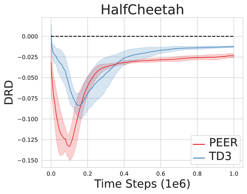
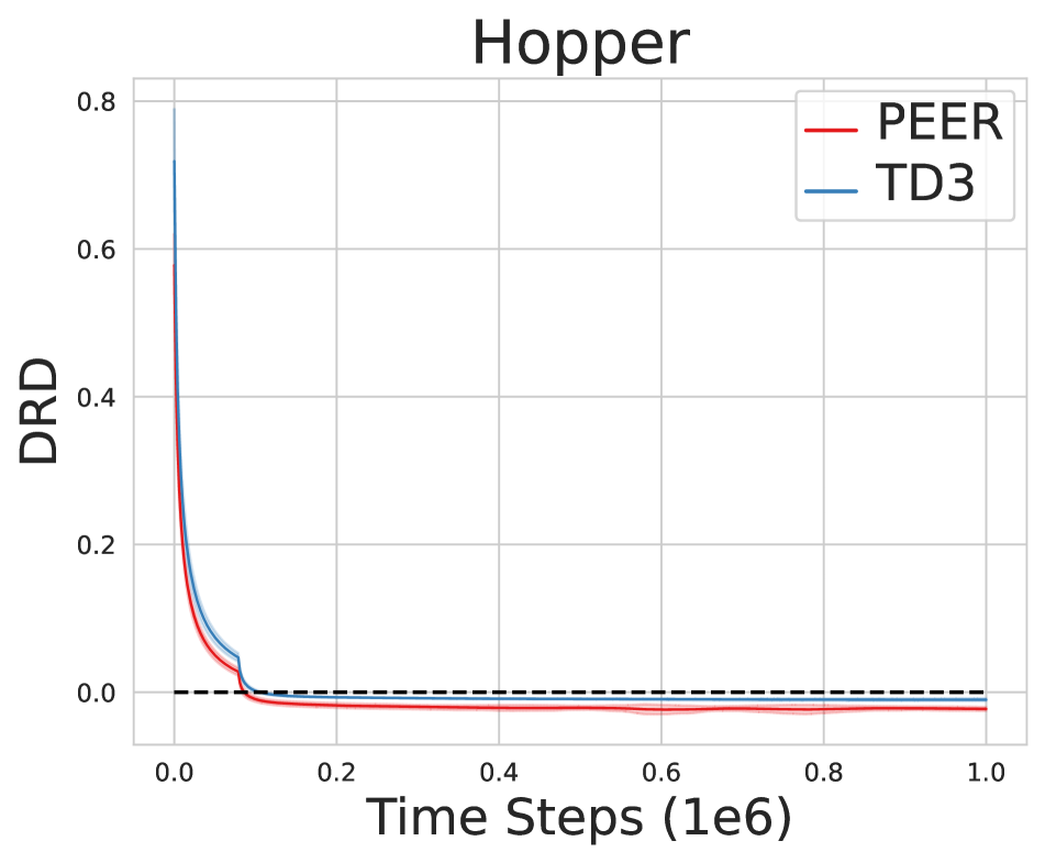
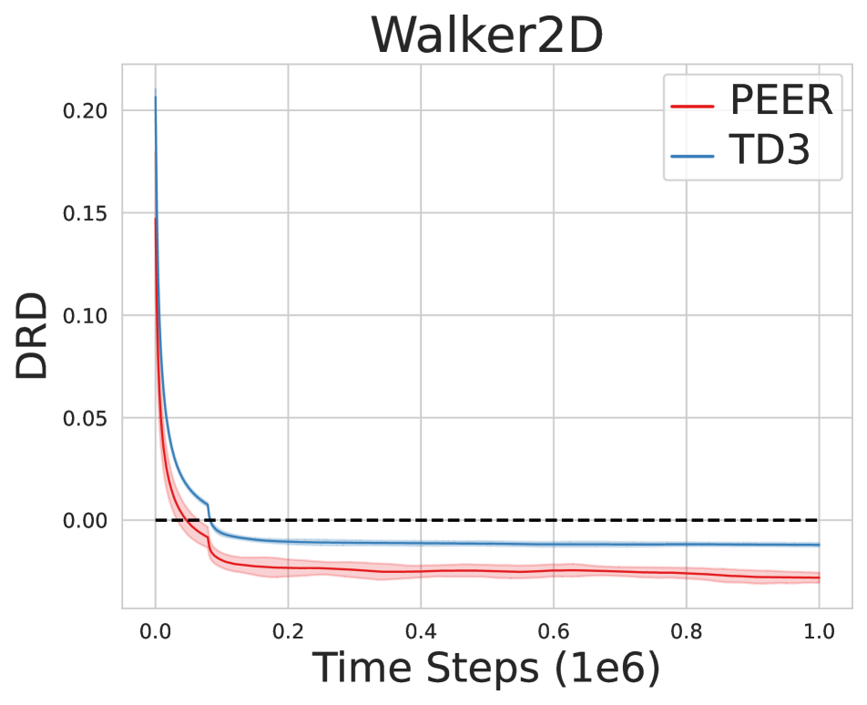
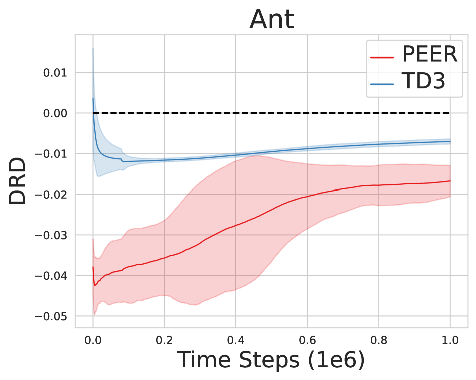
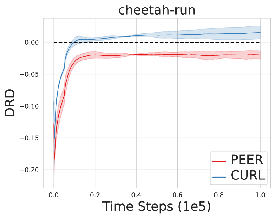
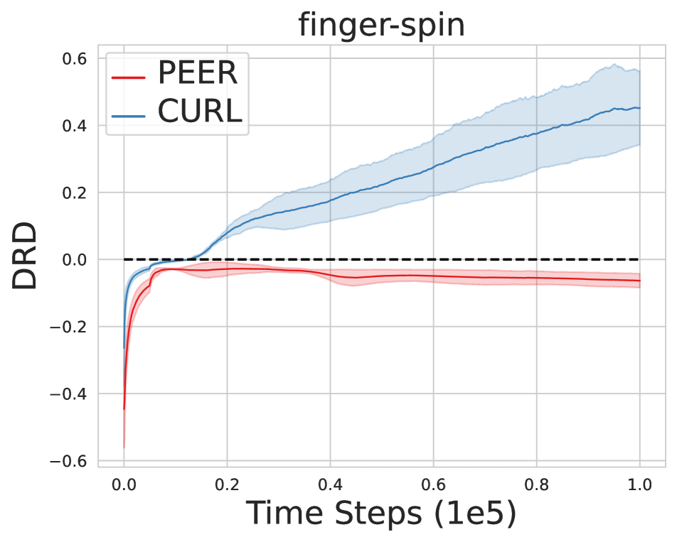
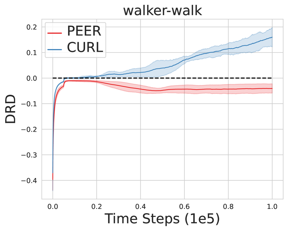
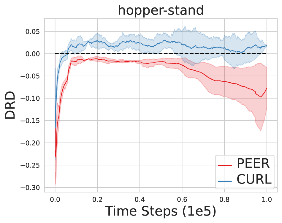
Figure 1: Distinguishable representation discrepancy (DRD) of TD3, CURL, and PEER agents on PyBullet and DMControl suites. TD3 agent does enjoy the distinguishable representation property. But the CURL agent does not satisfy the distinguishable representation property, which might negatively affect the model performance (see table 2). Not only does PEER enjoy the distinguishable representation property on state-based inputs environment bullets, but also in the pixel-based environment DMControl. The shaded area stands for a standard deviation.

3.1 Theoretical analysis

First of all, we theoretically examine the property that the internal representations of a Q-network and its target should satisfy under 3.1. Specifically, we show that the similarity of internal representations among two adjacent action-state pairs must be below a constant value, determined by both the neural network and reward function.

Assumption 3.1.

The $l_{2}$-norm of the representation is uniformly bounded by the square of some positive constant $G$, i.e. $\lVert\Phi(X;\Theta_{+})\rVert^{2}\leq G^{2}$ for any $X\in\mathcal{S}\times\mathcal{A}$ and network weights $\Theta$.

Theorem 3.2 (Distinguishable Representation Property).

The similarity (defined as inner product $\langle\cdot,\cdot\rangle$) between normalized representations $\Phi(s,a;\Theta_{+})$ of the $Q$-network and $\mathbb{E}_{s^{\prime},a^{\prime}}\Phi(s^{\prime},a^{\prime};\Theta^{\prime}_{+})$ satisfies

$$\langle\Phi(s,a;\Theta_{+}),\mathbb{E}_{s^{\prime},a^{\prime}}\Phi(s^{\prime},a^{\prime};\Theta^{\prime}_{+})\rangle\leq\frac{1}{\gamma}-\frac{r(s,a)^{2}}{2\lVert\Theta_{-1}\rVert^{2}},$$ (4)

where $s,a$ and $\Theta_{+}$ are state, action, and parameters of the $Q$-network except for those of the last layer. While $s^{\prime},a^{\prime},\Theta^{\prime}_{+}$ are the state, action at the next time step, and parameters of the target $Q$-network except for those of the last layer. And $\Theta_{-1}$ is the parameters of the last layer of $Q$-network.

Intuitively, theorem 3.2 indicates that the internal representations of different action-state pairs should be distinguishable so that the model is able to better pick the right action from action space. We define distinguishable representation discrepancy (DRD) as

$$\text{DRD}=\langle\Phi(s,a;\Theta_{+}),\mathbb{E}_{s^{\prime},a^{\prime}}\Phi(s^{\prime},a^{\prime};\Theta^{\prime}_{+})\rangle-\big{(}\frac{1}{\gamma}-\frac{r(s,a)^{2}}{2\lVert\Theta_{-1}\rVert^{2}}\big{)}.$$ (5)

We determine whether the internal representations of the Q-network and its target satisfy the distinguishable representation property by examining the value of DRD. If DRD $\leq 0$, then the property is satisfied; otherwise, it is not. Then, we evaluate whether this property is maintained by agents learned with two representative DRL methods, namely TD3 [28] and CURL [6] (without/with explicit representation learning techniques). The results are shown in fig. 1. From the results, we see that the TD3 agent does preserve the distinguishable representation property. While the CURL agent using explicit representation learning techniques does not satisfy the distinguishable representation property. This violation of the property could have a detrimental impact on agent performance (see section 4.2). These theoretical and experimental results motivate us to propose the following PEER regularization loss. This loss ensures that the learned model satisfies the distinguishable representation property through explicit regularization on representations.

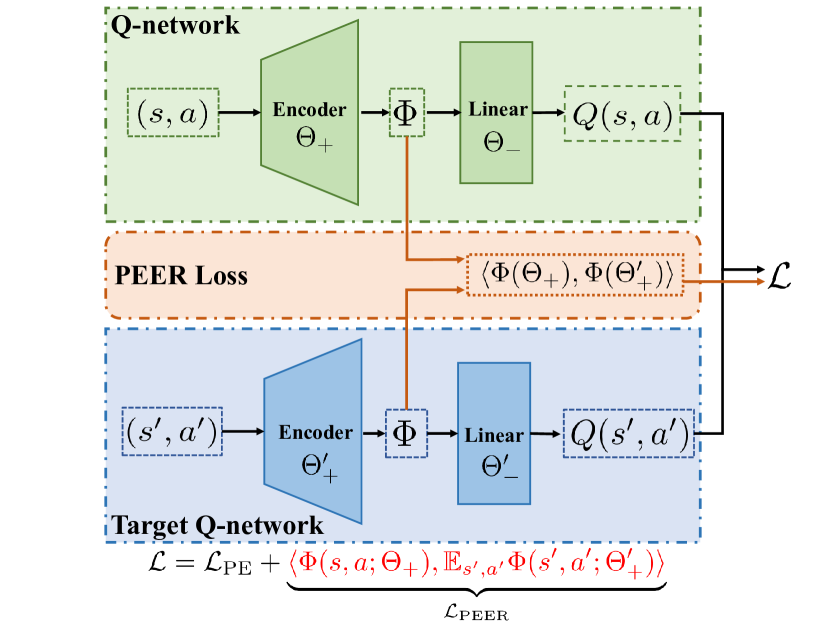
Figure 2: How the PEER loss is computed. The encoder is a nonlinear operator, and the state action pairs generate the representation $\Phi$ through the encoder and then the action value through a linear layer. PEER regularizes the policy evaluation phase by differing the representation $\Phi$ of the $Q$-network from that of its target. $\mathcal{L}_{\text{PE}}$ is a form of policy evaluation loss. And $\beta$ is a small positive constant, controlling the magnitude of the regularization effectiveness.

3.2 PEER

Specifically, the PEER loss is defined as

$$\mathcal{L}_{\text{ PEER}}(\Theta)=\langle\Phi(s,a;\Theta_{+}),\mathbb{E}_{s^{\prime},a^{\prime}}\big{[}\Phi(s^{\prime},a^{\prime};\Theta^{\prime}_{+})\big{]}\rangle,$$ (6)

where the $Q$-network takes the current state and action as inputs, and the inputs to the target network are the state and action at the next time step. This simple loss can be readily incorporated with the optimization objective of standard policy evaluation methods [35, 4, 2], leading to

$$\mathcal{L}(\Theta)=\mathcal{L}_{\text{PE}}(\Theta)+\beta\mathcal{L}_{\text{ PEER}}(\Theta),$$ (7)

where hyper-parameter $\beta$ controls the magnitude of the regularization effect of PEER. And $\mathcal{L}_{\text{PE}}(\Theta)$ is a policy evaluation phase loss e.g.

$$\mathcal{L}_{\text{PE}}(\Theta)=\Big{[}Q(s,a;\Theta)-\Big{(}r(s,a)+\gamma\mathbb{E}_{s^{\prime},a^{\prime}}\big{[}Q(s^{\prime},a^{\prime};\Theta^{\prime})\big{]}\Big{)}\Big{]}^{2}.$$

PEER can be combined with any DRL method that includes a policy evaluation phase, such as DQN [2], TD3, SAC [4]. Experiments presented in fig. 1 demonstrate that PEER maintains the distinguishable representation property. Furthermore, extensive experiments demonstrate PEER significantly improves existing algorithms by keeping the such property. The Pytorch-like pseudocode for the PEER loss can be found in Appendix section 8.3. And fig. 2 illustrates how the PEER loss is computed.

Convergence Guarantee.

We additionally provide a convergence guarantee of our algorithm. Following the definition in [36], let $\mathcal{F}$ be a class of measurable functions, a $\delta$-cover for $\mathcal{F}$ with $\delta>0$ is a finite set $\Gamma_{\delta}\subset\mathcal{F}$ such that $\forall f\in\mathcal{F}$, there exists $g\in\Gamma_{\delta}$ such that $\lVert f-g\rVert_{\infty}\leq\delta$, where $\lVert\cdot\rVert_{\infty}$ is the $l_{\infty}$-norm. A minimal $\delta$-cover is a $\delta$-cover and if taking out any of its elements, it is no longer a $\delta$-cover for $\mathcal{F}$. Let $T$ be the Bellman Operator. We have the following convergence result for the core update step in PEER.

Theorem 3.3 (One-step Approximation Error of the PEER Update).

Suppose 3.1 hold, let $\mathcal{F}\subset\mathcal{B}(\mathcal{S}\times\mathcal{A})$ be a class of measurable function on $\mathcal{S}\times\mathcal{A}$ that are bounded by $V_{\max}=R_{\max}/(1-\gamma)$, and let $\sigma$ be a probability distribution on $\mathcal{S}\times\mathcal{A}$. Also, let $\{(S_{i},A_{i})\}_{i\in[n]}$ be $n$ i.i.d. random variables in $\mathcal{S}\times\mathcal{A}$ following $\sigma$. For each $i\in[n]$, let $R_{i}$ and $S_{i}$ be the reward and the next state corresponding to $(s_{i},a_{i})$. In addition, for $Q\in\mathcal{F}$, we define $Y_{i}=R_{i}+\gamma\cdot\max_{a\in\mathcal{A}}Q(S^{\prime}_{i},a)$. Based on $\{(X_{i},A_{i},Y_{i})\}_{i\in[n]}$, we define $\hat{O}$ as the solution to the lease-square with regularization problem,

$$\min_{f\in\mathcal{F}}\frac{1}{n}\sum_{i=1}^{n}[f(S_{i},A_{i})-Y_{i}]^{2}+\beta\langle\Phi(s,a;\Theta),\mathbb{E}\Phi_{s^{\prime},a^{\prime}}(s^{\prime},a^{\prime};\Theta^{\prime})\rangle.$$ (8)

Meanwhile, for any $\delta>0$, let $\mathcal{N}(\delta,\mathcal{F},\lVert\cdot\rVert_{\infty})$ be the minimal $\delta$-covering set of $\mathcal{F}$ with respect to $l_{\infty}$-norm, and we denote by $N_{\delta}$ its cardinality. Then for any $\epsilon\in(0,1]$ and any $\delta>0$, we have

$$\lVert\hat{O}-TQ\rVert_{\sigma}^{2}\leq(1+\epsilon)^{2}\cdot\omega(\mathcal{F})+C\cdot V_{\max}^{2}/(n\cdot\epsilon)+C^{\prime}\cdot V_{\max}\cdot\delta+2\beta\cdot G^{2},$$ (9)

where $C$ and $C^{\prime}$ are two absolute constants and are defined as

$$\omega(\mathcal{F})=\sup_{g\in\mathcal{F}}\inf_{f\in\mathcal{F}}\lVert f-Tg\rVert_{\sigma}.$$ (10)

This result suggests the convergence rate of the previous result without PEER is maintained while PEER only adds a constant term $2\beta\cdot G^{2}$.

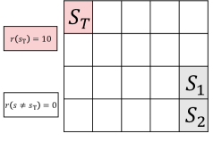
(a) Grid World

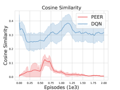
(b) Cosin similarity

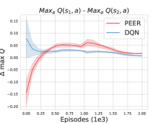
(c) Q value difference

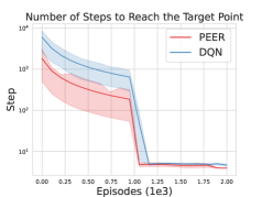
(d) Steps

Figure 3: Experiments on the grid world. (a) Grid world. We are interested in the values of $S_{1}$ and $S_{2}$. The policies are supposed to be able to differentiate the values of states $S_{1}$ and $S_{2}$ and tell that $S_{1}$ has the higher value. (b) The cosine similarity between the representation of the $Q$-network and its target. PEER (combined with DQN) effectively alleviates the similarity. (c) The difference between the max Q values of $S_{1}$ and $S_{2}$. Compared with DQN, PEER is able to better distinguish the Q values of two adjacent states by differentiating the representation of the $Q$-network and its target. (d) The number of steps to reach the $S_{T}$. PEER is better than DQN. The results are reported over five seeds and the shaded area represents a half standard deviation.

3.3 A toy example

We provide a toy example of a grid world (fig. 3(a)) to intuitively illustrate the functionality of PEER. In the grid world, the red state is the only state with a reward. We are interested in the Q values of the two gray states $S_{1}$ and $S_{2}$. Ideally, the policy is supposed to differentiate between those two adjacent states and accurately determine that $S_{1}$ has a higher value. We show the similarity between the representation of the $Q$-network and its target and the difference between the maximum Q value of two adjacent states in fig. 3. As shown in the fig. 3(b), PEER is able to better distinguish the representation of the $Q$-network and its target compared to DQN. Thus, PEER is better equipped to differentiate between the maximum Q values of the two nearby states $S_{1}$ and $S_{2}$ (fig. 3(c)). Consequently, PEER yields a better policy (fig. 3(d)).

4 Experiments

We perform comprehensive experiments to thoroughly assess PEER. Specifically, we evaluate (i) performance by measuring average returns on multiple suites when combined with different backbone algorithms; (ii) sample efficiency by comparing it with other algorithms at fixed timesteps; (iii) compatibility: whether PEER can be combined with other DRL algorithms such as off-policy methods TD3, contrastive unsupervised representation learning (CURL), and DrQ through extensive experiments; and (iv) the distinguishable representation property of PEER. To achieve this, we couple PEER with three representative DRL algorithms TD3 [28], CURL [6], and DrQ [9], and perform extensive experiments on four suites, namely, PyBullet, MuJoCo, DMControl, and Atari. PEER’s simplicity and ease of implementation are noteworthy, requiring only one line of code. We deliberately avoid using any engineering tricks that could potentially enhance its performance. This decision is made to ensure that the reproducibility crisis, which has been a growing concern in the field of DRL [37, 38], is not further exacerbated. We also maintain a fixed newly introduced hyper-parameter $\beta$ across all the experiments to achieve fair comparisons. Additional experimental details can be found in the Appendix.

4.1 Experimental settings

Hyper-parameters. We introduce only one additional hyper-parameter $\beta$ to control the magnitude of regularization effectiveness of PEER. We report all results using a fixed value of $\beta=5e-4$. It is important to note that PEER may benefit from selecting a $\beta$ value that is better suited to a specific environment.

Random seeds. To ensure the reproducibility of our experiments, we evaluate each tested algorithm using ten fixed random seeds unless otherwise specified. Moreover, we maintain fixed seeds across all experiments, including those used in PyTorch, Numpy, Gym, and CUDA packages.

Environments. To evaluate PEER, we use both state-based (state represented as vectors containing sensor information such as velocity, position, friction, etc) PyBullet and MuJoCo, and pixel-based (state represented as images) DMControl and Atari suites. The action space of PyBullet, MuJoCo, and DMControl is continuous, while that of Atari is discrete. Through the four experimental suites, we can check the performance and sample efficiency of PEER. We use the Gym [39] library for the interactive protocol. For PyBullet and MuJoCo suites, we run each tested algorithm for 1 million timesteps and evaluate the average return of the algorithm every 5k timesteps over ten episodes. For DMControl and Atari suites, following the commonly used experimental setting [6, 9], we measure the performance and sample-efficiency of tested algorithms at 100k and 500k environment timesteps, resulting in DMControl100k, DMControl500k, and Atari100k settings.

Algorithm	Ant	HalfCheetah	Hopper	Walker2D
PEER	3003 $\pm$ 204	2494 $\pm$ 276	2106 $\pm$ 164	1966 $\pm$ 58
TD3	2731 $\pm$ 278	2359 $\pm$ 229	1798 $\pm$ 471	1646 $\pm$ 314
METD3	2601 $\pm$ 246	2345 $\pm$ 151	1929 $\pm$ 351	1901 $\pm$ 111
SAC	2561 $\pm$ 146	1675 $\pm$ 567	1984 $\pm$ 103	1716 $\pm$ 30
PPO2	539 $\pm$ 25	397 $\pm$ 63	403 $\pm$ 70	390 $\pm$ 106
TRPO	693 $\pm$ 74	639 $\pm$ 154	1140 $\pm$ 469	496 $\pm$ 206

Table 1: The average return of the last ten evaluations over ten random seeds. PEER (coupled with TD3) outperforms all the compared algorithms, which shows that the PEER loss works in state-based environments. The best score is marked with colorbox. $\pm$ corresponds to a standard deviation over trials.

500K Step Scores	State SAC	PlaNet	Dreamer	SAC+AE	DrQ	DrQ-v2	CURL	PEER
Finger, Spin	923 $\pm$ 21	561 $\pm$ 284	796 $\pm$ 183	884 $\pm$ 128	938 $\pm$ 103	789 $\pm$ 124	926 $\pm$ 45	864 $\pm$ 160
Cartpole, Swingup	848 $\pm$ 15	475 $\pm$ 71	762 $\pm$ 27	735 $\pm$ 63	868 $\pm$ 10	845 $\pm$ 18	841 $\pm$ 45	866 $\pm$ 17
Reacher, Easy	923 $\pm$ 24	210 $\pm$ 390	793 $\pm$ 164	627 $\pm$ 58	942 $\pm$ 71	748 $\pm$ 229	929 $\pm$ 44	980 $\pm$ 3
Cheetah, run	795 $\pm$ 30	305 $\pm$ 131	570 $\pm$ 253	550 $\pm$ 34	660 $\pm$ 96	607 $\pm$ 32	518 $\pm$ 28	732 $\pm$ 41
Walker, Walk	948 $\pm$ 54	351 $\pm$ 58	897 $\pm$ 49	847 $\pm$ 48	921 $\pm$ 45	696 $\pm$ 370	902 $\pm$ 43	946 $\pm$ 17
Ball_in_cup, Catch	974 $\pm$ 33	460 $\pm$ 380	879 $\pm$ 87	794 $\pm$ 58	963 $\pm$ 9	844 $\pm$ 174	959 $\pm$ 27	973 $\pm$ 5
100K Step Scores
Finger, Spin	811 $\pm$ 46	136 $\pm$ 216	341 $\pm$ 70	740 $\pm$ 64	901 $\pm$ 104	325 $\pm$ 292	767 $\pm$ 56	820 $\pm$ 166
Cartpole, Swingup	835 $\pm$ 22	297 $\pm$ 39	326 $\pm$ 27	311 $\pm$ 11	759 $\pm$ 92	677 $\pm$ 214	582 $\pm$ 146	863 $\pm$ 17
Reacher, Easy	746 $\pm$ 25	20 $\pm$ 50	314 $\pm$ 155	274 $\pm$ 14	601 $\pm$ 213	256 $\pm$ 145	538 $\pm$ 233	961 $\pm$ 28
Cheetah, run	616 $\pm$ 18	138 $\pm$ 88	235 $\pm$ 137	267 $\pm$ 24	344 $\pm$ 67	273 $\pm$ 130	299 $\pm$ 48	499 $\pm$ 74
Walker, Walk	891 $\pm$ 82	224 $\pm$ 48	277 $\pm$ 12	394 $\pm$ 22	612 $\pm$ 164	171 $\pm$ 160	403 $\pm$ 24	714 $\pm$ 148
Ball_in_cup, Catch	746 $\pm$ 91	0 $\pm$ 0	246 $\pm$ 174	391 $\pm$ 82	913 $\pm$ 53	359 $\pm$ 228	769 $\pm$ 43	968 $\pm$ 7

Table 2: Scores achieved by PEER (coupled with CURL) on DMControl continuous control suite. PEER achieves superior performance on the majority (9 out of 12) tasks. And PEER also outperforms its backbone algorithm CURL on 11 out of 12 tasks by a large margin. The best score is marked with colorbox. $\pm$ corresponds to a standard deviation over trials.

Game	Human	Random	OTRainbow	Eff. Rainbow	Eff. DQN	DrQ	CURL	PEER+CURL	PEER+DrQ
Alien	7127.7	227.8	824.7	739.9	558.1	771.2	558.2	1218.9	712.7
Amidar	1719.5	5.8	82.8	188.6	63.7	102.8	142.1	185.2	163.1
Assault	742	222.4	351.9	431.2	589.5	452.4	600.6	631.2	721
Asterix	8503.3	210	628.5	470.8	341.9	603.5	734.5	834.5	918.2
BankHeist	753.1	14.2	182.1	51	74	168.9	131.6	78.6	12.7
BattleZone	37187.5	2360	4060.6	10124.6	4760.8	12954	14870	15727.3	5000
Boxing	12.1	0.1	2.5	0.2	-1.8	6	1.2	3.7	14.5
Breakout	30.5	1.7	9.8	1.9	7.3	16.1	4.9	3.9	8.5
ChopperCommand	7387.8	811	1033.3	861.8	624..4	780.3	1058.5	1451.8	1233.6
CrazyClimber	35829.4	10780.5	21327.8	16185.3	5430.6	20516.5	12146.5	18922.7	18154.5
DemonAttack	1971	152.1	711.8	508	403.5	1113.4	817.6	742.9	1236.7
Freeway	29.6	0	25	27.9	3.7	9.8	26.7	30.4	21.2
Frostbite	4334.7	65.2	231.6	866.8	202.9	331.1	1181.3	2151	537.4
Gopher	2412.5	257.6	778	349.5	320.8	636.3	669.3	583.6	681.8
Hero	30826.4	1027	6458.8	6857	2200.1	3736.3	6279.3	7499.9	3953.2
Jamesbond	302.8	29	112.3	301.6	133.2	236	471	414.1	213.6
Kangaroo	3035	52	605.4	779.3	448.6	940.6	872.5	1148.2	663.6
Krull	2665.5	1598	3277.9	2851.5	2999	4018.1	4229.6	4116.1	5444.7
KungFuMaster	22736.3	258.5	5722.2	14346.1	2020.9	9111	14307.8	15439.1	4090.9
MsPacman	6951.6	307.3	941.9	1204.1	872	960.5	1465.5	1768.4	1027.3
Pong	14.6	-20.7	1.3	-19.3	-19.4	-8.5	-16.5	-9.5	-18.2
PrivateEye	69571.3	24.9	100	97.8	351.3	-13.6	218.4	3207.7	8.2
Qbert	13455	163.9	509.3	1152.9	627.5	854.4	1042.4	2197.7	913.6
RoadRunner	7845	11.5	2696.7	9600	1491.9	8895.1	5661	10697.3	6900
Seaquest	42054.7	68.4	286.9	354.1	240.1	301.2	384.5	538.5	409.6
UpNDown	11693.2	533.4	2847.6	2877.4	2901.7	3180.8	2955.2	6813.5	7680.9

Table 3: Scores achieved by PEER (coupled with CURL and DrQ) and baselines on Atari. PEER achieves state-of-the-art performance on 19 out of 26 games. PEER implemented on top of CURL/DrQ improves over CURL/DrQ on 19/16 out of 26 games. Algorithms combined with PEER are reported across 10 random seeds. We also see that PEER achieves superhuman performance on Boxing, Freeway, JamesBond, Krull, and RoadRunner games. The best score is marked with colorbox.

Baselines. We first evaluate PEER on the state-based PyBullet suite, using TD3, SAC [4], TRPO [40], PPO[41] as our baselines for their superior performance. And we couple PEER with TD3 on PyBullet and MuJoCo experiments. PEER works as preventing the similarity between the representation of the Q-network and its target. Another relevant baseline is MEPG [42], which enforces a dropout operator on both the Q-network and its target. Dropout operator [43, 44] is generally believed to prevent feature co-adaptation, which is close to what PEER achieves. Therefore, we use MEPG combined with TD3 as a baseline, denoted as METD3. We employ the authors’ TD3 implementation, along with the public implementation [45] for SAC, and the Baselines codebase [46] for TRPO and PPO. We opt to adhere to the authors’ recommended default hyper-parameters for all considered algorithms.

Then we evaluate PEER on the pixel-based DMControl and Atari suites, combining it with CURL and DrQ algorithms. For DMControl, we select (i) PlaNet [5] and (ii) Dreamer [7], which learn a world model in latent space and execute planning; (iii) SAC+AE [8] uses VAE [47] and a regularized encoder; (iv) CURL using contrastive unsupervised learning to extract high-level features from raw pixels; (v) DrQ [9] and (vi) DrQ-v2 [18], which adopt data augmentation technique; and (vii) state-based SAC. For Atari suite, we select CURL, OTRainbow [48], Efficient Rainbow [49], Efficient DQN [9], and DrQ as baselines.

4.2 Results

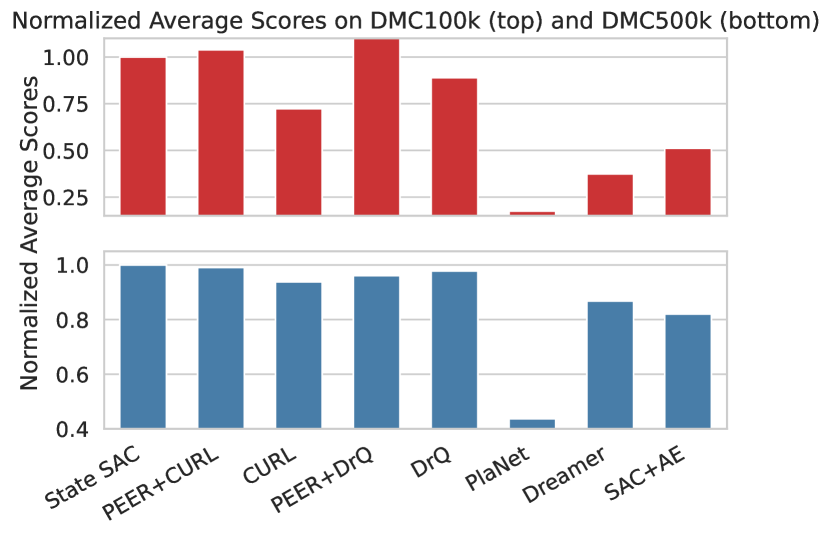
Figure 4: The normalized average scores on the DMControl suite. We normalize the average score of the tested algorithm by the average scores of State SAC. On the DMC100k benchmark, PEER (coupled with CURL and DrQ) outperforms all the compared algorithms including State SAC.

PyBullet. We first evaluate the PEER loss in the state-based suite PyBullet. We show the final ten evaluation average return in table 1. The results show (i) PEER coupled with TD3 outperforms TD3 on all environments. Furthermore, (ii) PEER also surpasses all other tested algorithms. The superior performance of PEER shows that the PEER loss can improve the empirical performance of the off-policy model-free algorithm that does not adopt any representation learning techniques.

DMControl. We then perform experiments on the DMControl suite. Specifically, we couple PEER with the CURL and DrQ algorithms, and run them in DMControl500k and DMControl100k settings. The results are shown in table 2 and fig. 4. The key findings are as follows: (i) On the DMControll500k setting, PEER coupled with CURL outperforms its backbone by a large margin on 5 out of 6 tasks, which shows the proposed PEER does improve the performance of its backbone algorithm. And the performance improvement on DMC500k shows that the PEER is beneficial for contrastive unsupervised learning (CURL). (ii) On the DMControl100k setting, The PEER (coupled with CURL) outperforms its backbone CURL on 6 out of 6 tasks. Besides, results in fig. 4 demonstrates that PEER (coupled with DrQ) improves the sample efficiency of DrQ by a large margin. Overall, the PEER achieves SOTA performance on 11 out of 12 tasks. (iii) PEER outperforms State SAC on 6 out of 12 tasks. In fig. 4, we computed the average score of the tested algorithm on all environments under DMControl100k and DMControl500k settings, normalized by the score of State SAC. The results in DMControl100k show that PEER (combined with CURL and DrQ) is more sample-efficient than State SAC and other algorithms. And in the DMControl500k suite, the sample efficiency of PEER matches that of State SAC. These results illustrate that PEER remarkably improves the empirical performance and sample efficiency of the backbone algorithms TD3, CURL, and DrQ.

Atari. We present Atari100k experiments in table 3, which show that (i) PEER achieves state-of-the-art performance on 19 out of 26 environments in given timesteps. And (ii) PEER implemented on top of CURL/DrQ improves over CURL on 19/16 out of 26 games. (iii) We also see that PEER achieves superhuman performance on Boxing, Freeway, JamesBond, Krull, and RoadRunner games. The empirical results demonstrate that PEER dramatically improves the sample efficiency of backbone algorithms.

4.3 Compatibility

Given a fixed hyper-parameter $\beta=5e-4$, PEER, as a plug-in, outperforms its backbone CURL algorithm on DMControl (11 out of 12) and Atari (19 out of 26) tasks, which shows that PEER is able to be incorporated into contrastive learn-based and data-augmentation methods to improve performance and sample efficiency. Besides, PEER coupled with DrQ also outperforms DrQ on 16 out of 26 environments. For state-based continuous control tasks, PEER (coupled with TD3) surpasses all the tested algorithms. These facts show that the compatibility of the PEER loss is remarkable and the PEER can be extended to incorporate more DRL algorithms. Theoretically, PEER tackles representation learning from the perspective of the representation of the Bellman equation, which is contrasting with other representation learning methods in DRL. Empirically, the performance of PEER loss coupled with representation learning DRL methods is better than that of backbone methods, which means that the PEER loss is orthogonal to other representation learning methods in DRL. Thus the compatibility of the PEER loss is auspicious.

4.4 PEER preserves distinguishable representation property

To validate whether the PEER regularizer preserves the distinguishable representation property or not, we measure the distinguishable representation discrepancy of the action value network and its target in PEER following section 3.1. We show the experimental results in fig. 1. The results show (i) TD3 and PEER (based on TD3) agents do enjoy the distinguishable representation property but that of PEER is more evident, which reveals the performance gain of PEER in this setting comes from better distinguishable representation property. (ii) The CURL agent does not maintain the distinguishable representation property on the tested DMControl suite, which negatively affects the model performance. And (iii) PEER also enjoys the distinguishable representation property on the pixel-based environment DMControl. Thus the performance of PEER is naturally improved due to the property being desirable. (iv) Combined with the performance improvement shown in performance experiments (section 4.2), PEER does improve the sample efficiency and performance by preserving the distinguishable representation property of the $Q$-network and its target.

5 Related Work

Representation learning [50, 51, 52, 53, 54, 16] aims at learning good or rich features of data. Such learned representation may be helpful for downstream tasks. The fields of natural language processing and computer vision have benefited from such techniques. It [19, 6, 9, 18, 20, 16] is widely acknowledged that good representations are conducive to improving the performance of DRL [55, 56, 35, 28, 4, 41, 42, 57]. Recent works [14, 15, 16, 6, 17, 9, 18] used self-supervised, unsupervised, contrastive representation learning, and data-augmentation approaches to improve the performance of DRL methods. There emerged several works studying representation learning from a geometric view [21, 22, 23]. Lyle et al. [24] explicitly considers representation capacity, which imposes regularization on the neural networks. The closest work to PEER is DR3 [58], which proposed a regularizer to tackle the implicit regularization effect of stochastic gradient descent in an offline RL setting. Despite the coincidental synergistic use of dot product form in PEER and DR3, we prove its necessity with different derivations and motivations. Our upper bound is rigorously derived for the representation of critic and its target network. But DR3 does not specify which network they select. DR3 only works in the offline setting, while PEER is, in theory, applicable to both online and offline settings.

Our work differentiates from previous works from the following three perspectives. First, PEER tackles representation learning by preserving the distinguishable representation property instead of learning good representations with the help of auxiliary tasks. The convergence rate guarantee of PEER can be proved. Second, the experiments show that PEER is orthogonal to existing representation learning methods in DRL. Third, PEER is also suitable for environments based on both states and pixels while other representation learning methods in DRL are almost only performed on pixel-based suites.

6 Conclusion

In this work, we initiated an investigation of the representation property of the $Q$-network and its target and found that they ought to satisfy an inherently favorable distinguishable representation property. Then illustrative experimental results demonstrate that deep RL agents may not be able to preserve this desirable property during training. As a solution to maintain the distinguishable representation property of deep RL agents, we propose a straightforward yet effective regularizer, PEER, and provide a convergence rate guarantee. Our extensive empirical results indicate that, with a fixed hyper-parameter, PEER exhibits superior improvements across all suites. Furthermore, the observed performance improvements are attributable to the preservation of distinguishable representational properties. Previous work on value function representations often makes the representations of adjacent moments similar, which is thought to maintain some smoothing. However, our work demonstrates that there is an upper bound on this similarity and that minimizing it can preserve a beneficial property, leading to sampling efficiency and performance improvements. In some cases, the performance of PEER is commensurate with that of State SAC. However, we leave the task of further analyzing the reasons for this parity for future research. To the best of our knowledge, PEER is the first work to study the inherent representation property of $Q$-network and its target. We believe that our work sheds light on the nature of the inherent representational properties arising from combining the parameterization tool neural networks and RL.

7 Appendix: Theoretical Derivation

Theorem 7.1 (Distinguishable Representation Property).

The similarity (defined as inner product $\langle\cdot,\cdot\rangle$) between normalized representations $\Phi(s,a;\Theta_{+})$ of the $Q$-network and $\mathbb{E}_{s^{\prime},a^{\prime}}\Phi(s^{\prime},a^{\prime};\Theta^{\prime}_{+})$ satisfies

$$\langle\Phi(s,a;\Theta_{+}),\mathbb{E}_{s^{\prime},a^{\prime}}\Phi(s^{\prime},a^{\prime};\Theta^{\prime}_{+})\rangle\leq\frac{1}{\gamma}-\frac{r(s,a)^{2}}{2\lVert\Theta_{-1}\rVert^{2}},$$ (11)

where $s,a$ and $\Theta_{+}$ are state, action, and parameters of the $Q$-network except for those of the last layer. While $s^{\prime},a^{\prime},\Theta^{\prime}_{+}$ are the state, action at the next time step, and parameters of the target $Q$-network except for those of the last layer. And $\Theta_{-1}$ is the parameters of the last layer of $Q$-network.

Proof.

Following eq. 3, the Bellman Equation eq. 2 can be rewritten as

$$\begin{split}\Phi(s,a;\Theta_{+})^{\top}\Theta_{-1}&=r(s,a)+\gamma\mathbb{E}_{s^{\prime},a^{\prime}}\Phi(s^{\prime},a^{\prime};\Theta^{\prime}_{+})^{\top}\Theta^{\prime}_{-1}.\end{split}$$ (12)

After the policy evaluation converges, $\Theta\text{ and }\Theta^{\prime}$ satisfy $\Theta=\Theta^{\prime}.$ Thus we have

$$\begin{split}(\Phi(s,a;\Theta_{+})^{\top}-\gamma\mathbb{E}_{s^{\prime},a^{\prime}}\Phi(s^{\prime},a^{\prime};\Theta^{\prime}_{+})^{\top})\Theta_{-1}&=r(s,a)\\ \lVert(\Phi(s,a;\Theta_{+})^{\top}-\gamma\mathbb{E}_{s^{\prime},a^{\prime}}\Phi(s^{\prime},a^{\prime};\Theta^{\prime}_{+})^{\top})\Theta_{-1}\rVert&=|r(s,a)|\\ \lVert(\Phi(s,a;\Theta_{+})^{\top}-\gamma\mathbb{E}_{s^{\prime},a^{\prime}}\Phi(s^{\prime},a^{\prime};\Theta^{\prime}_{+})^{\top})\rVert\lVert\Theta_{-1}\rVert\cos{\varphi}&=|r(s,a)|\\ \lVert(\Phi(s,a;\Theta_{+})^{\top}-\gamma\mathbb{E}_{s^{\prime},a^{\prime}}\Phi(s^{\prime},a^{\prime};\Theta^{\prime}_{+})^{\top})\rVert\lVert\Theta_{-1}\rVert&\geq|r(s,a)|\\ \lVert(\Phi(s,a;\Theta_{+})^{\top}-\gamma\mathbb{E}_{s^{\prime},a^{\prime}}\Phi(s^{\prime},a^{\prime};\Theta^{\prime}_{+})^{\top})\rVert&\geq\frac{|r(s,a)|}{\lVert\Theta_{-1}\rVert}.\\ \end{split}$$ (13)

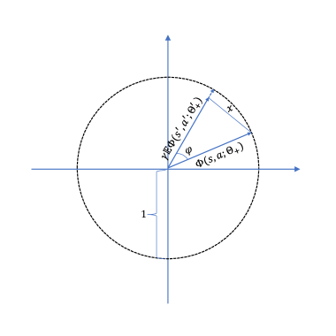
Figure 5: Normalized representation vectors.

Since the representation vectors are normalized, they should co-exist on some tangent plane as visualized in fig. 5. Let $x$ be $\|\Phi(s,a;\Theta_{+})-\gamma\mathbb{E}\Phi(s^{\prime},a^{\prime};\Theta^{\prime}_{+}\|$, then we have $x\geq\frac{|r(s,a)|}{\lVert\Theta_{-1}\rVert}$, and

$$\cos\varphi=\frac{\|\Phi(s,a;\Theta_{+})\|^{2}+\|\gamma\mathbb{E}\Phi(s^{\prime},a^{\prime};\Theta^{\prime}_{+})\|^{2}-x^{2}}{2\|\Phi(s,a;\Theta_{+})\|\|\gamma\mathbb{E}\Phi(s^{\prime},a^{\prime};\Theta^{\prime}_{+})\|}.$$ (14)

Now we have

$$\langle\Phi(s,a;\Theta_{+}),\gamma\mathbb{E}_{s^{\prime},a^{\prime}}\Phi(s^{\prime},a^{\prime};\Theta^{\prime}_{+})\rangle =\|\Phi(s,a;\Theta_{+})\|\|\gamma\mathbb{E}_{s^{\prime},a^{\prime}}\Phi(s^{\prime},a^{\prime};\Theta^{\prime}_{+})\|\cos\varphi$$ (15)

$$=1\cdot\|\gamma\mathbb{E}_{s^{\prime},a^{\prime}}\Phi(s^{\prime},a^{\prime};\Theta^{\prime}_{+})\|\cdot\frac{\|\Phi(s,a;\Theta_{+})\|^{2}+\|\gamma\mathbb{E}\Phi(s^{\prime},a^{\prime};\Theta^{\prime}_{+})\|^{2}-x^{2}}{2\|\Phi(s,a;\Theta_{+})\|\|\gamma\mathbb{E}\Phi(s^{\prime},a^{\prime};\Theta^{\prime}_{+})\|}$$

$$=\frac{1+\|\gamma\mathbb{E}\Phi(s^{\prime},a^{\prime};\Theta^{\prime}_{+})\|^{2}-x^{2}}{2}$$

$$\leq\frac{1+\gamma^{2}}{2}-\frac{r(s,a)^{2}}{2\lVert\Theta_{-1}\rVert^{2}}$$

$$\leq 1-\frac{r(s,a)^{2}}{2\lVert\Theta_{-1}\rVert^{2}}.$$

Thus, we have

$$\langle\Phi(s,a;\Theta_{+}),\mathbb{E}_{s^{\prime},a^{\prime}}\Phi(s^{\prime},a^{\prime};\Theta^{\prime}_{+})\rangle \leq\frac{1}{\gamma}-\frac{r(s,a)^{2}}{2\gamma\lVert\Theta_{-1}\rVert^{2}}$$ (16)

$$\leq\frac{1}{\gamma}-\frac{r(s,a)^{2}}{2\lVert\Theta_{-1}\rVert^{2}}.$$

∎

In the following, for notational simplicity, we use $X_{i}$ to denote $S_{i},A_{i}$ for all $i\in[n]$. For any $f\in\mathcal{F}$, $\lVert f\rVert_{n}^{2}=1/n\cdot\sum_{i=1}^{n}[f(X_{i})]^{2}$. Since both $\hat{O}$ and $TQ$ are bounded by $V_{\max}=R_{\max}/(1-\gamma)$, we only need to consider the case where $\log{N_{\delta}}\leq n$.

Let $f_{1},\cdots,f_{N_{\delta}}$ be the centers of minimal $\delta$-cover the of $\mathcal{F}$. By the definition of $\delta$-cover, there exists $k^{*}\in[N_{\delta}]$ such that $\lVert\hat{O}-f_{k^{*}}\rVert_{\infty}\leq\delta$. Notice that $k^{*}$ is a random variable since $\hat{O}$ is obtained from data.

Theorem 7.2 (One-step Approximation Error of PEER Update).

Suppose 3.1 hold, let $\mathcal{F}\subseteq\mathcal{B}(\mathcal{S}\times\mathcal{A})$ be a class of measurable function on $\mathcal{S}\times\mathcal{A}$ that are bounded by $V_{\max}=R_{\max}/(1-\gamma)$, and let $\sigma$ be a probability distribution on $\mathcal{S}\times\mathcal{A}$. Also, let $\{(S_{i},A_{i})\}_{i\in[n]}$ be $n$ i.i.d. random variables in following $\sigma$. Based on $\{(X_{i},A_{i},Y_{i})\}_{i\in[n]}$, we define $\hat{O}$ as the solution to the lease-square with regularization problem,

$$\min_{f\in\mathcal{F}}\frac{1}{n}\sum_{i=1}^{n}[f(S_{i},A_{i})-Y_{i}]^{2}+\beta\Phi(s,a;\Theta)\mathbb{E}\Phi_{s^{\prime},a^{\prime}}(s^{\prime},a^{\prime};\Theta^{\prime}).$$ (17)

At the same time, for any $\delta>0$, let $\mathcal{N}(\delta,\mathcal{F},\lVert\cdot\rVert_{\infty})$ be the

$$\lVert\hat{O}-TQ\rVert_{\sigma}^{2}\leq(1+\epsilon)^{2}\cdot\omega(\mathcal{F})+C\cdot V_{\max}^{2}/(n\cdot\epsilon)+C^{\prime}\cdot V_{\max}\cdot\delta+2\beta\cdot G^{2},$$ (18)

where $C$ and $C^{\prime}$ are two absolute constants and is defined as

$$\omega(\mathcal{F})=\sup_{g\in\mathcal{F}}\inf_{f\in\mathcal{F}}\lVert f-Tg\rVert_{\sigma}.$$ (19)

Proof.

Step (i): We relate $\mathbb{E}[\lVert\hat{O}-TQ\rVert_{n}^{2}]$ with its empirical counterpart $\lVert\hat{O}-TQ\rVert_{n}^{2}$. Since $Y_{i}=R_{i}+\gamma\max_{a\in\mathcal{A}}Q(S_{i+1},a)$ for each $i\in[n]$. By the definition of $\hat{O}$, for any $f\in\mathcal{F}$ we have

$$\sum_{i=1}^{n}[Y_{i}-\hat{O}(X_{i})]^{2}+\beta\Phi^{\top}(X_{i};\Theta_{\hat{O}})\mathbb{E}\Phi_{X_{i+1}}(X_{i+1};\Theta_{\hat{O}}^{\prime})\leq\sum_{i=1}^{n}[Y_{i}-f(X_{i})]^{2}+\beta\Phi^{\top}(X_{i};\Theta_{f})\mathbb{E}\Phi_{X_{i+1}}(X_{i+1};\Theta_{f}^{\prime}).$$ (20)

For each $i\in[n]$, we define $\xi_{i}=Y_{i}-(TQ)(X_{i})$. Then eq. 20 can be rewritten as

$$\begin{split}\lVert\hat{O}-TQ\rVert_{n}^{2}\leq\lVert f-TQ\rVert_{n}^{2}+\frac{1}{n}\sum_{i=1}^{n}\left[2\xi_{i}[\hat{O}(X_{i})-f(X_{i})]+\beta\left(\Phi^{\top}(X_{i};\Theta_{f})\mathbb{E}\Phi^{\top}(X_{i+1};\Theta_{f}^{\prime})-\Phi^{\top}(X_{i};\Theta_{\hat{O}})\mathbb{E}\Phi(X_{i+1};\Theta_{\hat{O}}^{\prime})\right)\right].\end{split}$$ (21)

We start by bounding the value of $\left(\Phi^{\top}(X_{i};\Theta_{f})\mathbb{E}\Phi(X_{i+1};\Theta_{f}^{\prime})-\Phi^{\top}(X_{i};\Theta_{\hat{O}})\mathbb{E}\Phi(X_{i+1};\Theta_{\hat{O}}^{\prime})\right)$. First, by Cauchy-Schwartz Inequality, we have

$$\left|\Phi(X_{i};\Theta_{f})\mathbb{E}\Phi(X_{i+1};\Theta_{f}^{\prime})\right|\leq\sqrt{\lVert\Phi(X_{i};\Theta_{f,+})\rVert^{2}}\cdot\sqrt{\lVert\mathbb{E}\Phi(X_{i+1};\Theta_{f,+}^{\prime})\rVert^{2}}\leq G^{2},$$ (22)

where we used 3.1 for the second inequality. Thus, by triangle inequality, we have

$$\left|\Phi^{\top}(X_{i};\Theta_{f})\mathbb{E}\Phi(X_{i+1};\Theta_{f}^{\prime})-\Phi(X_{i};\Theta_{\hat{O}})\mathbb{E}\Phi(X_{i+1};\Theta_{\hat{O}}^{\prime}\right|\leq 2G^{2}.$$ (23)

And eq. 21 reduces to

$$\lVert\hat{O}-TQ\rVert_{n}^{2}\leq\lVert f-TQ\rVert_{n}^{2}+\frac{2}{n}\sum_{i=1}^{n}\left[\xi_{i}[\hat{O}(X_{i})-f(X_{i})]+\beta G^{2}\right].$$ (24)

Then we bound the rest on the right side of eq. 21. Since both $f$ and $Q$ are deterministic, we have $\mathbb{E}(\lVert f-TQ\rVert^{2}_{n})=\lVert f-TQ\rVert^{2}_{\sigma}$. Moreover, since $\mathbb{E}(\xi_{i}|X_{i})=0$ by definition, we have $\mathbb{E}[\xi_{i}\cdot g(X_{i})]=0$ for any bounded and measurable function $g$. Thus it holds that

$$\mathbb{E}\left\{\sum_{i=1}^{n}\xi_{i}\cdot[\hat{O}(X_{i})-f(X_{i})]\right\}=\mathbb{E}\left\{\sum_{i=1}^{n}\xi_{i}\cdot[\hat{O}-(TQ)(X_{i})]\right\}.$$ (25)

In addition, by triangle inequality and eq. 25 we have

$$\left|\mathbb{E}\left\{\sum_{i=1}^{n}\xi_{i}\cdot[\hat{O}(X_{i})-(TQ)(X_{i})]\right\}\right|\leq\left|\mathbb{E}\left\{\sum_{i=1}^{n}\xi_{i}\cdot[\hat{O}-f_{k^{*}}(X_{i})]\right\}\right|+\left|\mathbb{E}\left\{\sum_{i=1}^{n}\xi_{i}\cdot[f_{k^{*}}(X_{i})-(TQ)(X_{i})]\right\}\right|,$$ (26)

where $f_{k*}$ satisfies $\lVert f_{k*}\rVert\leq\delta$. In the following, we upper bound the two terms on the right side of eq. 26 respectively. For the first term, by applying the Cauchy-Schwarz inequality twice, we have

$$\begin{split}\left|\mathbb{E}\left\{\sum_{i=1}^{n}\xi_{i}\cdot[\hat{O}-f_{k^{*}}(X_{i})]\right\}\right|&\leq\sqrt{n}\cdot\left|\mathbb{E}\left[\left(\sum_{i=1}^{n}\xi_{i}^{2}\right)^{1/2}\cdot\lVert\hat{O}-f_{k^{*}}\rVert_{n}\right]\right|\\ &\leq\sqrt{n}\cdot[\mathbb{E}(\sum_{i=1}^{n}\xi_{i}^{2})]^{1/2}\cdot[\mathbb{E}(\lVert\hat{O}-f_{k^{*}}\rVert_{n}^{2})]^{1/2}\leq n\delta\cdot[\mathbb{E}(\xi_{i}^{2})]^{1/2}.\end{split}$$ (27)

where we use the fact that $\{\xi_{i}\}_{i\in[n]}$ have the same marginal distributions and $\lVert\hat{O}-f_{k*}\rVert_{n}\leq\delta$. Since both $Y_{i}$ and $TQ$ are bounded by $V_{\max}$, $\xi_{i}$ is a bounded random variable by its definition. Thus, there exists a constant $C_{\xi}>0$ depending on $\xi$ such that $\mathbb{E}(\xi_{i}^{2})\leq C_{\xi}^{2}\cdot V_{\max}^{2}$. Then eq. 27 implies

$$\left|\mathbb{E}\left\{\sum_{i=1}^{n}\xi_{i}\cdot[\hat{O}(X_{i})-f_{k^{*}}(X_{i})]\right\}\right|\leq C_{\xi}\cdot V_{\max}\cdot n\delta.$$ (28)

It remains to upper bound the second term on the right side of eq. 26. We define $N_{\delta}$ self-normalized random variables

$$Z_{j}=\frac{1}{\sqrt{n}}\sum_{i=1}^{n}\xi_{i}\cdot[f_{j}(X_{i})-(TQ)(X_{i})]\cdot\lVert f_{j}-(TQ)\rVert_{n}^{-1}$$ (29)

for all $j\in[N_{\delta}]$. Here recall that $\left\{f_{j}\right\}_{j\in[N_{\delta}]}$ are the centers of the minimal $\delta$-covering of $\mathcal{F}$. Then we have

$$\begin{split}\left|\mathbb{E}\left\{\sum_{i=1}^{n}\xi_{i}\cdot[f_{k*}(X_{i})-(TQ)(X_{i})]\right\}\right|&=\sqrt{n}\cdot\mathbb{E}[{\lVert f_{k^{*}}-TQ\rVert_{n}}\cdot|Z_{k^{*}}|]\\ &\leq\sqrt{n}\cdot\mathbb{E}\left\{[\lVert\hat{O}-TQ\rVert_{n}+\lVert\hat{O}-f_{k^{*}}\rVert_{n}]\cdot|Z_{k^{*}}|\right\}\leq\sqrt{n}\cdot\left\{[\lVert\hat{O}-TQ\rVert_{n}+\delta]\cdot|Z_{k^{*}}|\right\},\end{split}$$ (30)

where the first inequality follows from triangle inequality and the second follows from the fact that $\leq\delta$ eq. 30, we obtain

$$\begin{split}\mathbb{E}\left\{[\lVert\hat{O}-TQ\rVert_{n}+\delta]\cdot|Z_{k^{*}}|\right\}&\leq\left(\mathbb{E}\left\{[\lVert\hat{O}-TQ\rVert_{n}+\delta]^{2}\right\}\right)^{1/2}\cdot[\mathbb{E}(Z_{k^{*}}^{2})]^{1/2}\\ &\leq\left(\left\{\mathbb{E}[\lVert\hat{O}-TQ\rVert_{n}^{2}]\right\}^{1/2}+\delta\right)\cdot[\mathbb{E}(\max_{j\in[n]}Z_{j}^{2})]^{1/2},\end{split}$$ (31)

where the last inequality follows from

$$\mathbb{E}[{\lVert\hat{O}-TQ\rVert_{n}}]\leq\left\{\mathbb{E}[\lVert\hat{O}-TQ\rVert_{n}^{2}]\right\}^{1/2}.$$ (32)

Moreover, since $\xi_{i}$ is centered conditioning on $\left\{X_{i}\right\}$, $\xi_{i}$ is a sub-Gaussian random variable. Specifically, there exists an absolute constant $H_{\xi}>0$ such that $\lVert\xi_{i}\rVert_{\psi_{2}}\leq H_{\xi}\cdot V_{\max}$ for each $i\in[n]$. Here the $\psi_{2}$-norm of a random variable $W$ is defined as

$$\lVert W\rVert_{\psi_{2}}=\sup_{p\geq 1}p^{-1/2}[\mathbb{E}({|W|^{p}})]^{1/p}.$$ (33)

By the definition of $Z_{j}$ in eq. 29, conditioning on $\left\{X_{i}\right\}_{i\in[n]}$, $\xi_{i}\cdot[f_{j}(X_{i})-(TQ)(X_{i})]$ is a centered and sub-Guassian random variable with

$$\lVert\xi_{i}\cdot[f_{j}(X_{i})-TQ(X_{i})]\rVert_{\psi_{2}}\leq H_{\xi}\cdot V_{\max}\cdot|f_{j}(X_{i})-(TQ)(X_{i})|.$$ (34)

Moreover, since $Z_{j}$ is a summation of independent sub-Gaussian random variables, by Lemma 5.9 of [59], the $\psi_{2}$-norm of $Z_{j}$ satisfies

$$\lVert Z_{j}\rVert_{\psi_{2}}\leq C\cdot H_{\xi}\cdot V_{\max}\cdot\lVert f_{j}-TQ\rVert_{n}^{-1}\cdot\left[\frac{1}{n}\sum_{i=1}^{n}|[f_{j}(X_{i})-(TQ)(X_{i})]|^{2}\right]^{1/2}\leq C\cdot H_{\xi}\cdot V_{\max},$$ (35)

where $C>0$ is an absolute constant. Furthermore, by Lemma 5.14 and 5.15 of [59], $Z_{j}^{2}$ is a sub-exponential random variable, and its moment-generating function is bounded by

$$\mathbb{E}\left[\exp(t\cdot Z_{j}^{2})\right]\leq\exp(C\cdot t^{2}\cdot H_{\xi}^{4}\cdot V_{\max}^{4})$$ (36)

for any $t$ satisfying $C^{\prime}\cdot|t|\cdot H_{\xi}^{2}\cdot V_{\max}^{2}\leq 1$, where $C$ and $C^{\prime}$ are two positive absolute constants. Moreover, by Jensen’s Inequality, we bound the moment-generating function of $\max_{j\in[N_{\delta}]}Z_{j}^{2}$ by

$$\mathbb{E}\left[\exp(t\cdot\max_{j\in[N_{\delta}]}Z_{j}^{2})\right]\leq\sum_{j\in[N_{\delta}]}\mathbb{E}[\exp(t\cdot Z_{j}^{2})].$$ (37)

Combining eq. 36 and eq. 37, we have

$$\mathbb{E}(\max_{j\in[N]}Z_{j}^{2})\leq C^{2}\cdot H_{\xi}^{2}\cdot V_{\max}^{2}\cdot\log{N_{\delta}},$$ (38)

where $C>0$ is an absolute constant. Hence, plugging eq. 38 into eq. 30 and eq. 31, we upper bound the second term of eq. 25 by

$$\begin{split}\left|\mathbb{E}\left\{\sum_{i=1}^{n}\xi_{i}\cdot[f_{k^{*}}(X_{i})-(TQ)(X_{i})]\right\}\right|&\leq\left(\left\{\mathbb{E}\lVert\hat{O}-TQ\rVert_{n}^{2}\right\}^{1/2}+\delta\right)\cdot C\cdot H_{\xi}\cdot V_{\max}\cdot\sqrt{n\cdot\log{N_{\delta}}}.\end{split}$$ (39)

Finally, combining eq. 24, eq. 28 and eq. 39, we obtain the following inequality

$$\begin{split}\mathbb{E}[\lVert\hat{O}-TQ\rVert_{n}^{2}]&\leq\inf_{f\in\mathcal{F}}\mathbb{E}[\lVert f-TQ\rVert_{n}^{2}]+C_{\xi}\cdot V_{\max}\cdot\delta\\ &+\left(\left\{\mathbb{E}\lVert\hat{O}-(TQ)\rVert\right\}^{1/2}+\delta\right)\cdot C\cdot H_{\xi}\cdot V_{\max}+\sqrt{\log{N_{\delta}/n}}+2\cdot\beta\cdot G^{2}\\ &\leq C\cdot V_{\max}\sqrt{\log{N_{\delta}/n}}+\inf_{f\in\mathcal{F}}\mathbb{E}[\lVert f-TQ\rVert_{n}^{2}]+C^{\prime}\cdot V_{\max}\delta+2\cdot\beta\cdot G^{2},\end{split}$$ (40)

where $C$ and $C^{\prime}$ are two constants. Here in the first inequality we take the infimum over $\mathcal{F}$ because eq. 20 holds for any $f\in\mathcal{F}$, and the second inequality holds because $\log{N_{\delta}}\leq n$.

Now we invoke a fact to obtain the final bound for $\mathbb{E}[\lVert\hat{O}-TQ\rVert_{n}^{2}]$ from eq. 40. Let $a,b$ and $c$ be positive numbers satisfying $a^{2}\leq 2ab+c$. For any $\epsilon\in(0,1]$, since $2ab\leq\frac{\epsilon}{1+\epsilon}a^{2}+\frac{1+\epsilon}{\epsilon}b^{2}$, we have

$$a^{2}\leq(1+\epsilon)^{2}\cdot b^{2}/\epsilon+(1+\epsilon)\cdot c.$$ (41)

Therefore, applying eq. 41 to eq. 40 with $a^{2}=\mathbb{E}[\lVert\hat{O}-TQ\rVert_{n}^{2}]$, $b=C\cdot V_{\max}\cdot\sqrt{\log{N}}$ and $c=\inf_{f\in\mathcal{F}}\mathbb{E}[\lVert f-TQ\rVert_{n}^{2}]+C^{\prime}\cdot V_{\max}\cdot\delta$, we obtain

$$\mathbb{E}[\lVert\hat{O}-TQ\rVert_{n}^{2}]\leq(1+\epsilon)\cdot\inf_{f\in\mathcal{F}}\mathbb{E}[\lVert f-TQ\rVert_{n}^{2}]+C\cdot V_{\max}^{2}\cdot\log{N_{\delta}}/(n\epsilon)+C^{\prime}\cdot V_{\max}\cdot\delta+2\beta G^{2},$$ (42)

where $C$ and $C^{\prime}$ are two positive absolute constants. This concludes the first step.

Step (ii): In this step, we relate the population risk $\lVert\hat{O}-TQ\rVert^{2}_{\delta}$ with $\mathbb{E}[\lVert\hat{O}-TQ\rVert^{2}_{n}]$, which is bounded in the first step. To begin with, we generate $n$ i.i.d. random variables $\left\{\tilde{X}_{i}=(\tilde{S}_{i},\tilde{A}_{i})\right\}_{i\in[n]}$ following $\sigma$, independent of $\{(S_{i},A_{i},R_{i},S^{\prime}_{i})\}_{i\in[n]}$. Since $\lVert\hat{O}-f_{k^{*}}\rVert_{\infty}\leq\delta$, for any $x\in\mathcal{S}\times\mathcal{A}$, we have

$$\begin{split}\left|[\hat{O}(x)-(TQ)(x)]^{2}-[f_{k^{*}}(x)-(TQ)(x)]^{2}\right|=\left|\hat{O}(x)-f_{k^{*}}(x)\right|\cdot\left|\hat{O}(x)+f_{k^{*}}(x)-2(TQ)(x)\right|\leq 4V_{\max}\cdot\delta,\end{split}$$ (43)

where the last inequality follows from the fact that $\lVert TQ\rVert_{\infty}\leq V_{\max}$ and $\lVert f\rVert_{\infty}\leq V_{\max}$ for any $f\in\mathcal{F}$.

Then by the definition of $\lVert\hat{O}-TQ\rVert^{2}_{\delta}$ and eq. 43, we have

$$\begin{split}\lVert\hat{O}-TQ\rVert_{\sigma}^{2}&=\mathbb{E}\left\{\frac{1}{n}\sum_{i=1}^{n}[\hat{O}(\tilde{X_{i}})-(TQ)(\tilde{X_{i}})]^{2}\right\}\\ &\leq\mathbb{E}\left\{\lVert\hat{O}-TQ\rVert^{2}_{n}+\frac{1}{n}\sum_{i=1}^{n}[f_{k^{*}}(\tilde{X_{i}})-(TQ)(\tilde{X_{i}})]^{2}-\frac{1}{n}\sum_{i=1}^{n}[f_{k^{*}}(X_{i})-(TQ)(\tilde{X_{i}})]^{2}\right\}+8V_{\max}\cdot\delta\\ &=\mathbb{E}(\lVert\hat{O}-TQ\rVert^{2}_{n})+\mathbb{E}[\frac{1}{n}\sum^{n}h_{k^{*}}(X_{i},\tilde{X_{i}})]+8V_{\max}\cdot\delta,\end{split}$$ (44)

where we apply eq. 43 to obtain the first inequality, and in the last equality we define

$$h_{j}(x,y)=[f_{j}(y)-(TQ)(y)]^{2}-[f_{j}(x)-(TQ)(x)]^{2},$$ (45)

for any $x,y\in\mathcal{S}\times\mathcal{A}$ and any $j\in[N_{\delta}]$. Note that $h_{k^{*}}$ is a random function since $k^{*}$ is random. By the definition of $h_{j}$, we have $|h_{j}(x,y)|\leq 4V_{\max}^{2}$ for any $(x,y)\in\mathcal{S}\times\mathcal{A}$ and $\mathbb{E}[h_{j}(X_{i},\tilde{X}_{i})]=0$ for any $i\in[n]$. Moreover, the variance of $h_{j}(X_{i},\tilde{X_{i}})$ satisfies

$$\begin{split}\operatorname{Var}[h_{j}(X_{i},\tilde{X_{i}})]&=2\operatorname{Var}{\left\{[f_{j}(X_{i})-(TQ)(X_{i})]^{2}\right\}}\\ &\leq 2\mathbb{E}\left\{[f_{j}(X_{i})-(TQ)(X_{i})]^{4}\right\}\leq 8\Upsilon^{2}\cdot V_{\max}^{2},\end{split}$$ (46)

where we define $\Upsilon$ by letting

$$\Upsilon=\max(4V_{\max}^{2}\cdot\log{N_{\delta}/n},\max_{j\in[N_{\delta}]}\mathbb{E}\left\{[f_{j}(X_{i})-(TQ)(X_{i})]^{2}\right\}).$$ (47)

Furthermore, we define

$$T=\sup_{j\in[N_{\delta}]}\left|\sum_{i=1}^{n}h(X_{i},\tilde{X_{i}})/\Upsilon\right|.$$ (48)

Combining eq. 44 and eq. 48,

$$\lVert\hat{O}-TQ\rVert_{\sigma}^{2}\leq\mathbb{E}[\lVert\hat{O}-TQ\rVert_{n}^{2}]+\Upsilon/n\cdot\mathbb{E}[T]+8V_{\max}\cdot\delta.$$ (49)

In the following, we use Bernstein’s Inequality to establish an upper bound for $\mathbb{E}(T)$:

Lemma 7.3.

(Bernstein’s Inequality) Let $U_{1},\cdots,U_{n}$ be n independent random variables satisfying $\mathbb{E}(U_{i})=0$ and $\leq$ for all $i\in[n]$. Then for any $t>0$, we have

$$\mathbb{P}\left(\left|\sum_{i=1}^{n}U_{i}\right|\geq t\right)\leq 2\exp(\frac{-t^{2}}{2M\cdot t/3+2\sigma^{2}}),$$ (50)

where $\sigma^{2}=\sum_{i=1}^{n}$ is the variance of $\sum_{i=1}^{n}U_{i}$.

We first apply Bernstein’s Inequality by setting $U_{i}=h_{j}(X_{i},\tilde{X_{i}})/\Upsilon$ for each $i\in[n]$. Then we take a union bound for all $j\in[N_{\delta}]$ to obtain

$$\mathbb{P}(T\geq t)=\mathbb{P}\left[\sup_{j\in[N_{\delta}]}\frac{1}{n}\left|\sum_{i=1}^{n}h_{j}(X_{i},\tilde{X_{i}})/\Upsilon\right|\geq t\right]\leq 2N_{\delta}\cdot\exp\left\{\frac{-t^{2}}{8V_{\max}^{2}\cdot[t/(3\Upsilon)+n]}\right\}.$$ (51)

Since $T$ is nonnegative, $\mathbb{E}(T)=\int_{0}^{\infty}\mathbb{P}(T\geq t)dt$. Thus, for any $u\in(0,3\Upsilon\cdot n)$,

$$\begin{split}\mathbb{E}(T)&\leq u+\int_{u}^{\infty}\mathbb{P}(T\geq t)\,dt\leq u+2N_{\delta}\int_{u}^{3\Upsilon\cdot n}\exp\left(\frac{-t^{2}}{16V_{\max}^{2}\cdot n}\right)\,dt+2N_{\delta}\int_{3\Upsilon\cdot n}^{\infty}\exp{\left(\frac{-3\Upsilon\cdot t}{16V_{\max}^{2}}\right)}\,dt\\ &\leq u+32N_{\delta}\cdot V_{\max}\cdot n/u\cdot\exp\left(\frac{-u^{2}}{16V_{\max}^{2}\cdot n}\right)+32N_{\delta}\cdot V_{\max}^{2}/(3\Upsilon)\cdot\exp{\left(\frac{-9\Upsilon^{2}\cdot n}{16V_{\max}^{2}}\right)},\end{split}$$ (52)

where in the second inequality we use the fact that $\int_{s}^{\infty}\exp{(-t^{2}/2)}dt\leq 1/s\cdot\exp(-s^{2}/2)$. Now we set $u=4V_{\max}\sqrt{n\cdot\log{N_{\delta}}}$ in eq. 52 and plug in the definition of $\Upsilon$ in eq. 46 to obtain

$$\mathbb{E}\leq 4V_{\max}\log{n\cdot N_{\delta}}+8V_{\max}\sqrt{n/\log{N_{\delta}}}+6V_{\max}\sqrt{n/\log{N_{\delta}}}\leq 8V_{\max}\sqrt{n\cdot\log{N_{\delta}}},$$ (53)

where the last inequality holds when $\log{N_{\delta}}\geq 4$. Moreover, the definition of $\Upsilon$ in eq. 46 implies that $\Upsilon\leq\max[2V_{\max}\sqrt{\log{N_{\delta}/n}},\lVert\hat{O}-TQ\rVert^{2}_{\sigma}+\delta]$. In the following, we only need to consider the case where $\Upsilon\leq\lVert\hat{O}-TQ\rVert_{\sigma}+\delta$, since we already have eq. 18 if $\lVert\hat{O}-TQ\rVert+\delta\leq 2V_{\max}\sqrt{\log{N_{\delta}/n}}$, which concludes the proof.

Then, when $\Upsilon\leq\lvert\hat{O}-TQ\rVert_{\sigma}+\delta$ holds, combining eq. 49 and eq. 53 we have,

$$\begin{split}\lVert\hat{O}-TQ\rVert_{\delta}^{2}&\leq\mathbb{E}[\lVert\hat{O}-TQ\rVert_{n}^{2}]+8V_{\max}\sqrt{\log{N_{\delta}}/n}\cdot\lVert\hat{O}-TQ\rVert_{\delta}+8V_{\max}\sqrt{\log{N_{\delta}/n}}\cdot\delta+8V_{\max}\cdot\delta\\ &\leq\mathbb{E}[\lVert\hat{O}-TQ\rVert_{n}^{2}]+8V_{\max}\sqrt{\log{N_{\delta}/n}}\cdot\lVert\hat{O}-TQ\rVert_{\sigma}+16V_{\max}\cdot\delta.\end{split}$$ (54)

We apply the inequality in eq. 41 to eq. 54 with $a=\lVert\hat{O}-TQ\rVert_{\sigma}$, $b=8V_{\max}\sqrt{\log{N_{\delta}}/n}$, and $c=\mathbb{E}[\lVert\hat{O}-TQ\rVert_{n}^{2}]+16V_{\max}\cdot\delta$ we have. Hence we found

$$\begin{split}\lVert\hat{O}-TQ\rVert_{\sigma}^{2}\leq(1+\epsilon)\cdot\mathbb{E}[\lVert\hat{O}-TQ\rVert_{n}^{2}]+(1+\epsilon)^{2}\cdot 64V_{\max}\cdot\log{N_{\delta}}/(n\cdot\epsilon)+(1+\epsilon)\cdot 18V_{\max}\cdot\delta,\end{split}$$ (55)

which concludes the second step of the proof.

Finally, combining steps (i) and together, i.e., eq. 42 and eq. 55, we conclude that

$$\lVert\hat{O}-TQ\rVert_{\sigma}^{2}\leq(1+\epsilon)^{2}\cdot\inf_{f\in\mathcal{F}}\mathbb{E}[\lVert f-TQ\rVert^{2}_{n}]+C_{1}\cdot V_{\max}^{2}\cdot\log{N_{\delta}/(n\cdot\epsilon)}+C_{2}\cdot V_{\max}\cdot\delta+2\beta G^{2},$$ (56)

where $C_{1}$ and $C_{2}$ are two absolute constants. Moreover, since $Q\in\mathcal{F}$

$$\inf_{f\in\mathcal{F}}\mathbb{E}[\lVert f-TQ\rVert_{n}^{2}]\leq\sup_{Q\in\mathcal{F}}\left\{\inf_{f\in\mathcal{F}}\mathbb{E}[\lVert f-TQ\rVert_{n}^{2}]\right\},$$ (57)

which concludes the proof of theorem 3.3. ∎

8 Appendix: Experimental Settings

In this section, we provide the experimental settings in detail.

8.1 Code

Our project is available at https://sites.google.com/view/peer-cvpr2023/.

8.2 Experimental Details

Our implementation of PEER coupled with CURL/DrQ is based on the CURL/DrQ codebase.

Computational resources. All experiments are conducted on two GPU servers. The first one has 3 Titan XP GPUs and Intel(R) Xeon(R) CPU E5-2640 v4 @ 2.40GHz. The second one has 4 Titan RTX GPUs and an Intel(R) Xeon(R) Gold 6137 CPU @ 3.90GHz. Each run for DMControl takes fifty hours to finish. For PyBullet, MuJoCo, and Atari tasks, it takes 5 hours to finish a run. For PyBullet and MuJoCo suites, we simultaneously launch 70 seeds. For the DMControl and Atari suites, we simultaneously run 15 random seeds.

How to plot fig. 1. Before computing the distinguishable representation discrepancy (DRD), the representation of $Q$-network is normalized as shown in theorem 7.1. Then we compute DRD in mini-batch samples. We compute the average DRD of mini-batch samples, and plot fig. 1 over five random seeds.

The source of data in table 2. The evaluation results of State SAC, PlaNet, Dreamer, SAC+AE, and CURL in table 2 are taken from the original CURL paper [6]. And the results of DrQ are taken from the original DrQ paper [9]. As for the data of DrQ-v2, we took from the authors’ data (link: https://github.com/facebookresearch/drqv2) and presented the statistics in the same way as the rest of table 2. Note that the author only provides DrQ-v2 results over nine seeds.

The source of data in table 3. The evaluation results of Human, Random, OTRainbow, Eff.Rainbow, and CURL in table 3 are taken from the original CURL paper [6]. And the results of Eff. DQN and DrQ are taken from the original DrQ paper [9].

Data in fig. 4. We do not include the DrQ-v2 results in fig. 4 because DrQ is better than DrQ-v2 as shown in table 2.

Random seeds. If not otherwise specified, we evaluate each tested algorithm over 10 random seeds to ensure the reproducibility of our experiments. Also, we set all seeds fixed in our experiments.

Grid world. The grid world is shown in fig. 3(a). If the agent arrives at $S_{T}$, it gets a reward of 10, and other states get a reward of 0. We present the remaining hyper-parameters for the grid world in table 4.

PyBullet. When we train the agent on the Pybullet suite, the agent starts by randomly collecting 25,000 states and actions for better exploration. Then we evaluate the agent for ten episodes every 5,000 timesteps. We take the average return of ten episodes as a key evaluation metric. To ensure a fair evaluation of the algorithms, we do not apply any exploration tricks during the evaluation phase (e.g. injecting noise into actions in TD3), because these exploration tricks may harm the performance of tested algorithms. The complete timesteps are 1 million. The results are reported over ten random seeds. For the hyper-parameter $\beta$ of PEER, we take $5e-4$ for every task.

For all algorithms except METD3, we use the author’s implementation [28] or a commonly used public repository [46]. Our implementations of PEER and METD3 are based on TD3 implementation. To fairly evaluate our algorithm, we keep all the original TD3’s hyper-parameters without any modification. For the hyper-parameter of METD3, we set the dropout rate equal to $0.1$ as the author [42] did. The soft update style is adopted for METD3, PEER with $\eta=0.005$. We summarize the hyper-parameter settings for the PyBullet suite in table 5.

MuJoCo. All experiments on MuJoCo are consistent with the PyBullet settings, except for the code of SAC used. We found that the performance of SAC [45] deteriorates on the MuJoCo suite. Therefore, we use the code of Stable-Baselines3 [60] for SAC implementation with the same hyper-parameters under PyBullet settings.

DMControl. We utilize the authors’ implementation of CURL and DrQ without any further modification as we discussed. And we do not change the default hyper-parameters for CURL. For a fair comparison, we keep the hyper-parameters of PEER the same as CURL and DrQ. And the hyper-parameter $\beta=5e-4$ is kept in each environment. We summarize the hyper-parameter settings for the DMControl suite in table 6 and table 7.

Atari. Our implementation PEER is based on CURL. For a fair comparison, we keep the hyper-parameters and settings of CURL the same as CURL. And the hyper-parameter $\beta=5e-4$ is kept in each environment. Check table 8 and table 9 for more details.

8.3 Pseudocode for PEER Loss

We provide PyTorch-like pseudocode for the PEER loss as follows.

⬇

1def PE_loss_with_PEER(representation, Q, target_representation, target_Q, beta):

2 """

3 representation: shape = Batch_size * N, representation of critic

4 Q: shape = Batch_size * 1, current Q value

5 target_representation: shape = Batch_size * N, representation of critic_target

6 target_Q: shape = Batch_size * 1, target Q value ( r + \mathcal{E}Q(s’,a’) )

7 beta: a small constant, controlling the regularization effectiveness of PEER

8 """

9 PEER_loss = torch.einsum(’ij,ij->i’, [representation, target_representation]).mean()

10 PE_loss = torch.nn.functional.mse_loss(Q, target_Q).mean()

11

12 loss = PE_loss + beta * PEER_loss

13 return loss

Listing 1: Pytorch-like pseudocode for the PEER loss

Hyper-parameter	Value
Shared hyper-parameters
State space	integer: from 0 to 19
Action space	Discrete(4): up, down, left, right
Discount ($\gamma$)	0.99
Replay buffer size	$10^{5}$
Optimizer	Adam [61]
Learning rate for Q-network	$1\times 10^{-4}$
Number of hidden layers for all networks	2
Number of hidden units per layer	32
Activation function	ReLU
Mini-batch size	64
Random starting exploration time steps	$10^{3}$
Target smoothing coefficient ($\eta$)	0.005
Gradient Clipping	False
Exploration Method	Epsilon-Greedy
$\epsilon$	0.1
Evaluation Episode	10
Number of Episodes	2000
PEER
PEER coefficient ($\beta$)	$5\times 10^{-4}$

Table 4: Hyper-parameters settings for Grid World experiments

Hyper-parameter	Value
Shared hyper-parameters
Discount ($\gamma$)	0.99
Replay buffer size	$10^{6}$
Optimizer	Adam [61]
Learning rate for actor	$3\times 10^{-4}$
Learning rate for critic	$3\times 10^{-4}$
Number of hidden layers for all networks	2
Number of hidden units per layer	256
Activation function	ReLU
Mini-batch size	256
Random starting exploration time steps	$2.5\times 10^{4}$
Target smoothing coefficient ($\eta$)	0.005
Gradient Clipping	False
Target update interval ($d$)	2
TD3
Variance of exploration noise	0.2
Variance of target policy smoothing	0.2
Noise clip range	$[-0.5,0.5]$
Delayed policy update frequency	2
PEER
PEER coefficient ($\beta$)	$5\times 10^{-4}$
SAC
Target Entropy	- dim of $\mathcal{A}$
Learning rate for $\alpha$	$1\times 10^{-4}$

Table 5: Hyper-parameters settings for PyBullet and MuJoCo experiments

Hyper-parameter	Value
PEER coefficient ($\beta$)	$5\times 10^{-4}$
Discount $\gamma$	0.99
Replay buffer size	100000
Optimizer	Adam
Learning rate	$1\times 10^{-4}$
Learning rate $\left(f_{\theta},\pi_{\psi},Q_{\phi}\right)$	$2\times 10^{-4}$ cheetah, run
	1 $\times 10^{-3}$ otherwise
Convolutional layers	4
Number of filters	32
Activation function	ReLU
Encoder EMA $\eta$	0.05
Q function EMA ($\eta$)	0.01
Mini-batch size	512
Target Update interval $(d)$	2
Latent dimension	50
Initial temperature	0.99
Number of hidden units per layer ( MLP )	1024
Evaluation episodes	10
Random crop	True
Observation rendering	(100,100)
Observation downsampling	(84,84)
Initial steps	1000
Stacked frames	3
Action repeat	2 finger, spin; walker, walk
	8 cartpole, swingup
	4 otherwise
$\left(\beta_{1},\beta_{2}\right)\rightarrow\left(f_{\theta},\pi_{\psi},Q_{\phi}\right)$	(.9, .999)
$\left(\beta_{1},\beta_{2}\right)\rightarrow(\alpha)$	(.9, .999)

Table 6: Hyper-parameters settings for PEER (coupled with CURL) DMControl experiments.

Hyper-parameter	Value
PEER coefficient ($\beta$)	$5\times 10^{-4}$
Replay buffer capacity	$100000$
Seed steps	$1000$
Main results minibatch size	$512$
Discount $\gamma$	$0.99$
Optimizer	Adam
Learning rate	$10^{-3}$
Critic target update frequency	$2$
Critic Q-function soft-update rate $\tau$	$0.01$
Actor update frequency	$2$
Actor log stddev bounds	$[-10,2]$
Init temperature	$0.1$

Table 7: Hyper-parameters settings for PEER (coupled with DrQ) DMControl experiments.

Hyper-parameter	Value
PEER coefficient ($\beta$)	$5\times 10^{-4}$
Random crop	True
Image size	$(84,84)$
Data Augmentation	Random Crop (Train)
Replay buffer size	$100000$
Training frames	$400000$
Training steps	$100000$
Frame skip	$4$
Stacked frames	$4$
Action repeat	$4$
Replay period every	$1$
Q network: channels	$32$, $64$
Q network: filter size	$5\times 5,5\times 5$
Q network: stride	$5$, $5$
Q network: hidden units	$256$
Momentum (EMA for CURL) $\tau$	$0.001$
Non-linearity	ReLU
Reward Clipping	$[-1,1]$
Multi step return	$20$
Minimum replay size for sampling	$1600$
Max frames per episode	$108$K
Update	Distributional Double Q
Target Network Update Period	every $2000$ updates
Support-of-Q-distribution	$51$ bins
Discount $\gamma$	$0.99$
Batch Size	$32$
Optimizer	Adam
Optimizer: learning rate	$0.0001$
Optimizer: $\beta 1$	$0.9$
Optimizer: $\beta 2$	$0.999$
Optimizer $\epsilon$	$0.000015$
Max gradient norm	$10$
Exploration	Noisy Nets
Noisy nets parameter	$0.1$
Priority exponent	$0.5$
Priority correction	$0.4\rightarrow 1$
Hardware	GPU

Table 8: Hyper-parameters used for Atari100K PEER (coupled with CURL) experiments.

Hyperparameter	Value
PEER coefficient ($\beta$)	$5\times 10^{-4}$
Data augmentation	Random shifts and Intensity
Grey-scaling	True
Observation down-sampling	$84\times 84$
Frames stacked	$4$
Action repetitions	$4$
Reward clipping	$[-1,1]$
Terminal on loss of life	True
Max frames per episode	$108$k
Update	Double Q
Dueling	True
Target network: update period	$1$
Discount factor	$0.99$
Minibatch size	$32$
Optimizer	Adam
Optimizer: learning rate	$0.0001$
Optimizer: $\beta_{1}$	$0.9$
Optimizer: $\beta_{2}$	$0.999$
Optimizer: $\epsilon$	$0.00015$
Max gradient norm	$10$
Training steps	$100$k
Evaluation steps	$125$k
Min replay size for sampling	$1600$
Memory size	Unbounded
Replay period every	$1$ step
Multi-step return length	$10$
Q network: channels	$32,64,64$
Q network: filter size	$8\times 8$, $4\times 4$, $3\times 3$
Q network: stride	$4,2,1$
Q network: hidden units	$512$
Non-linearity	ReLU
Exploration	$\epsilon$-greedy
$\epsilon$-decay	$5000$

Table 9: Hyper-parameters used for Atari100K PEER (coupled with DrQ algorithm) experiments.

9 Appendix: Experimental Suites

The experimental suites we use are Bullet [29], MuJoCo[31], DMcontrol[30], and Atari[32]. We show the environments of bullet, MuJoCo, DMControl, and Atari in fig. 6, fig. 7, fig. 8, fig. 9, and fig. 10, respectively.

Besides, We list the state and action information for the four suites in table 10, table 11, table 12, and table 13. respectively.

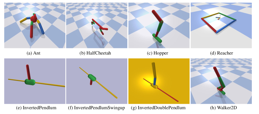
Figure 6: Images for PyBullet suite used in our experiments. The states for this suite are vectors.

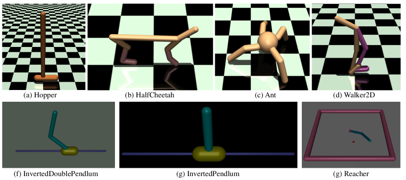
Figure 7: Images for MuJoCo suite used in our experiments. The states for this suite are vectors.

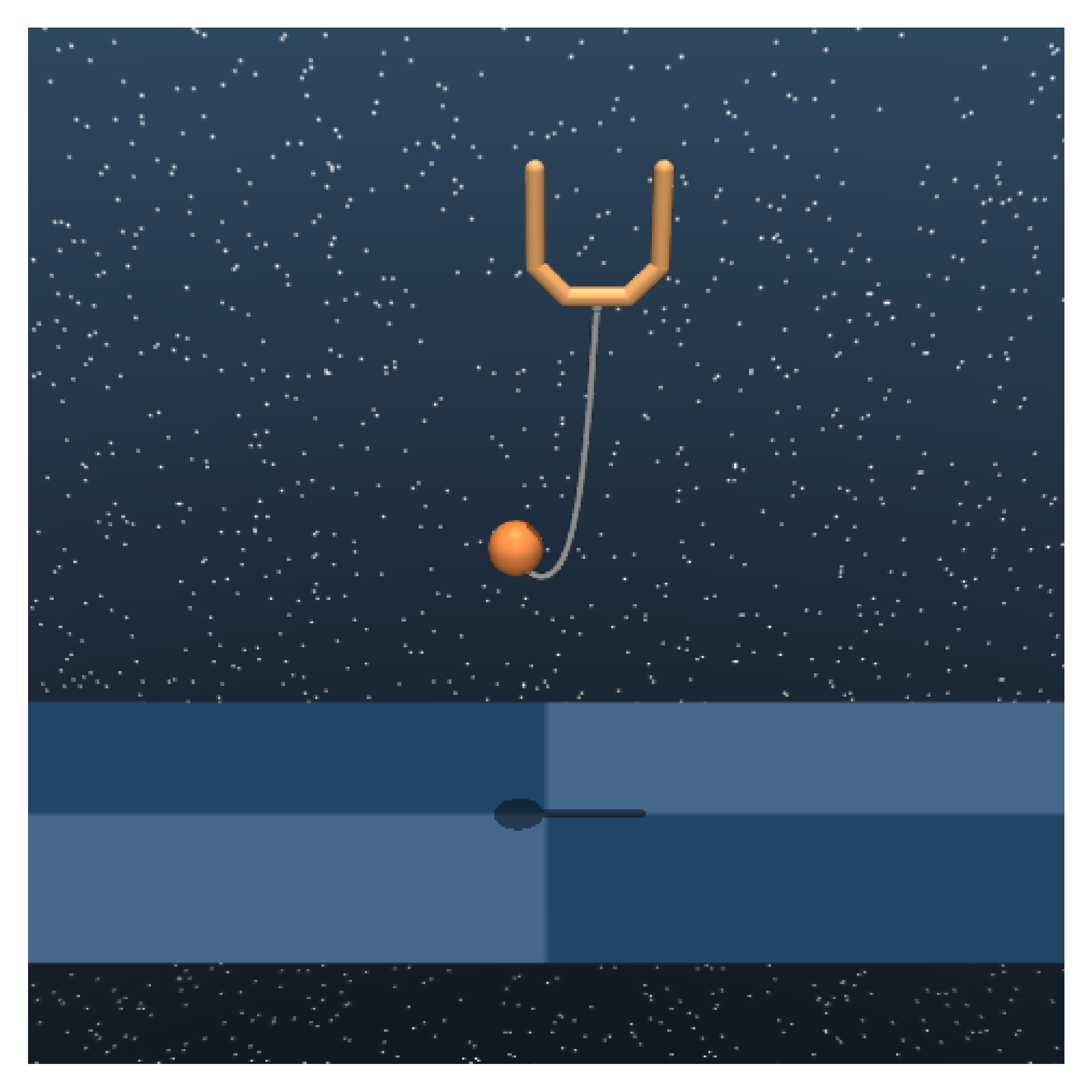
(a) ball_in_cup_catch

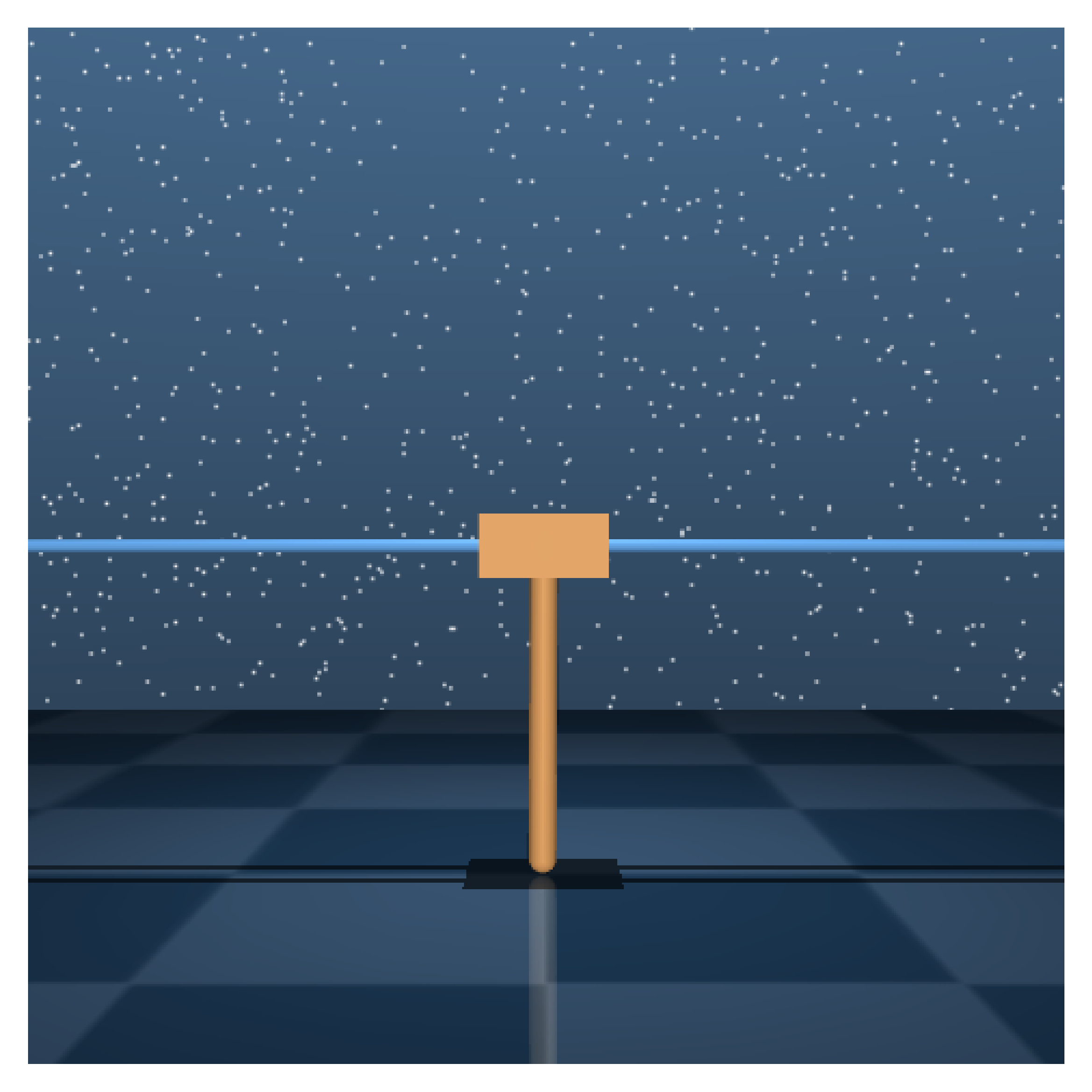
(b) cartpole_swingup

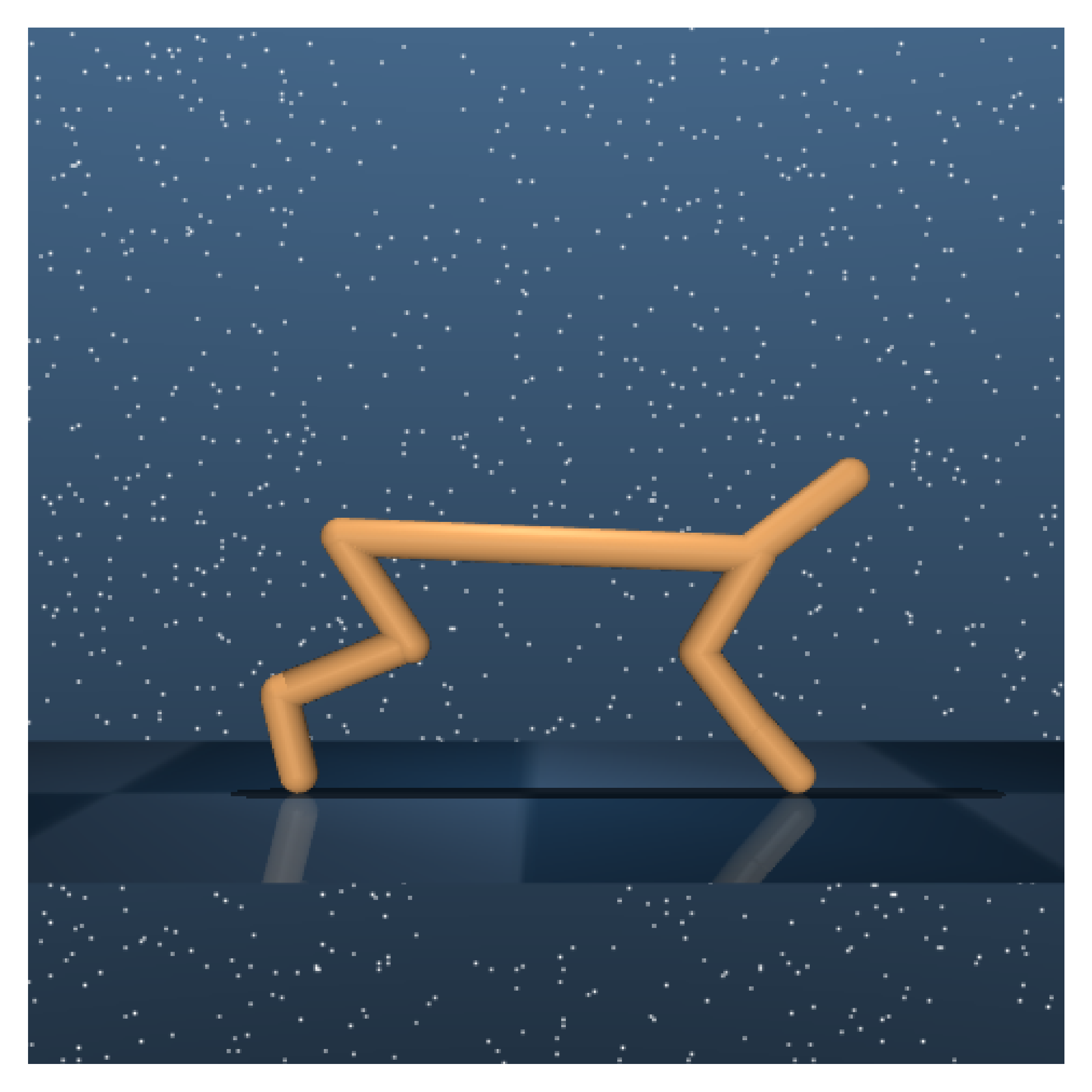
(c) cheetah_run

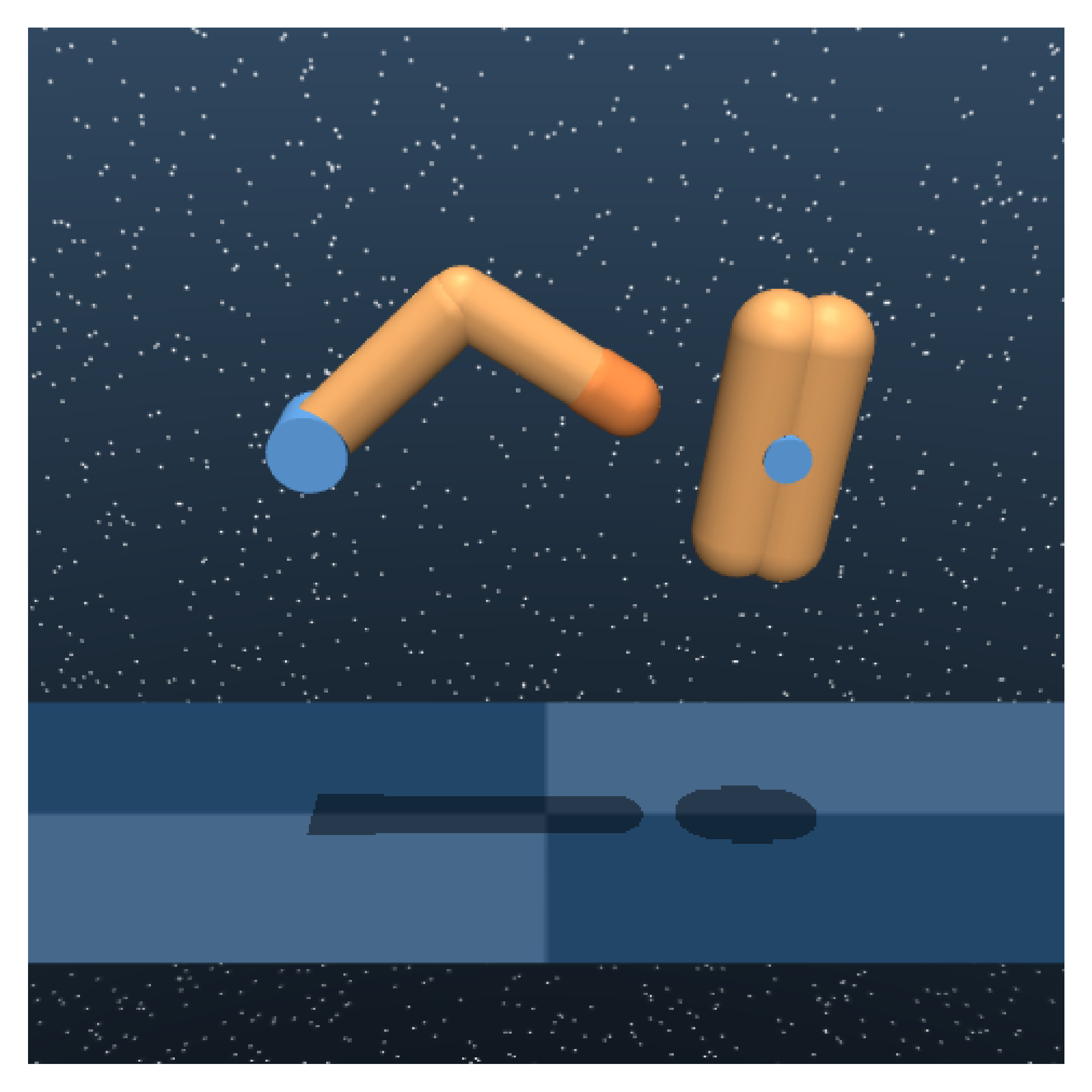
(d) finger_spin

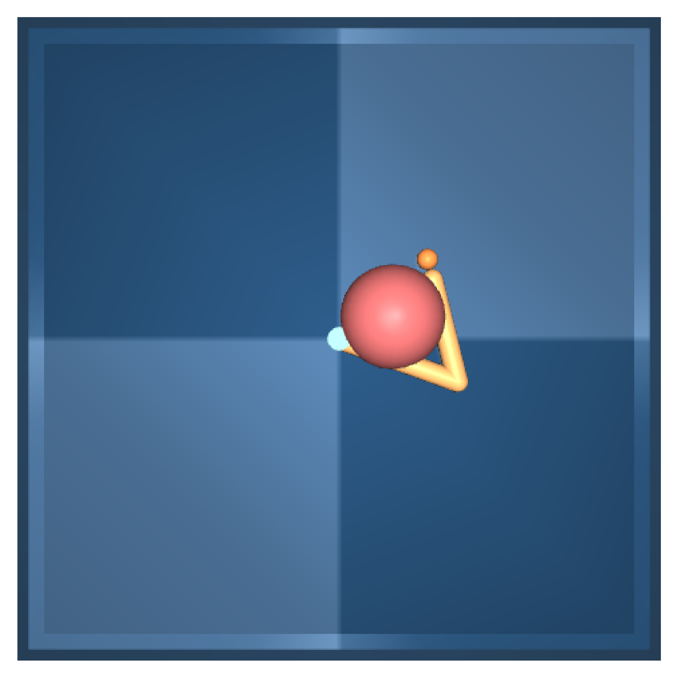
(e) reacher_easy

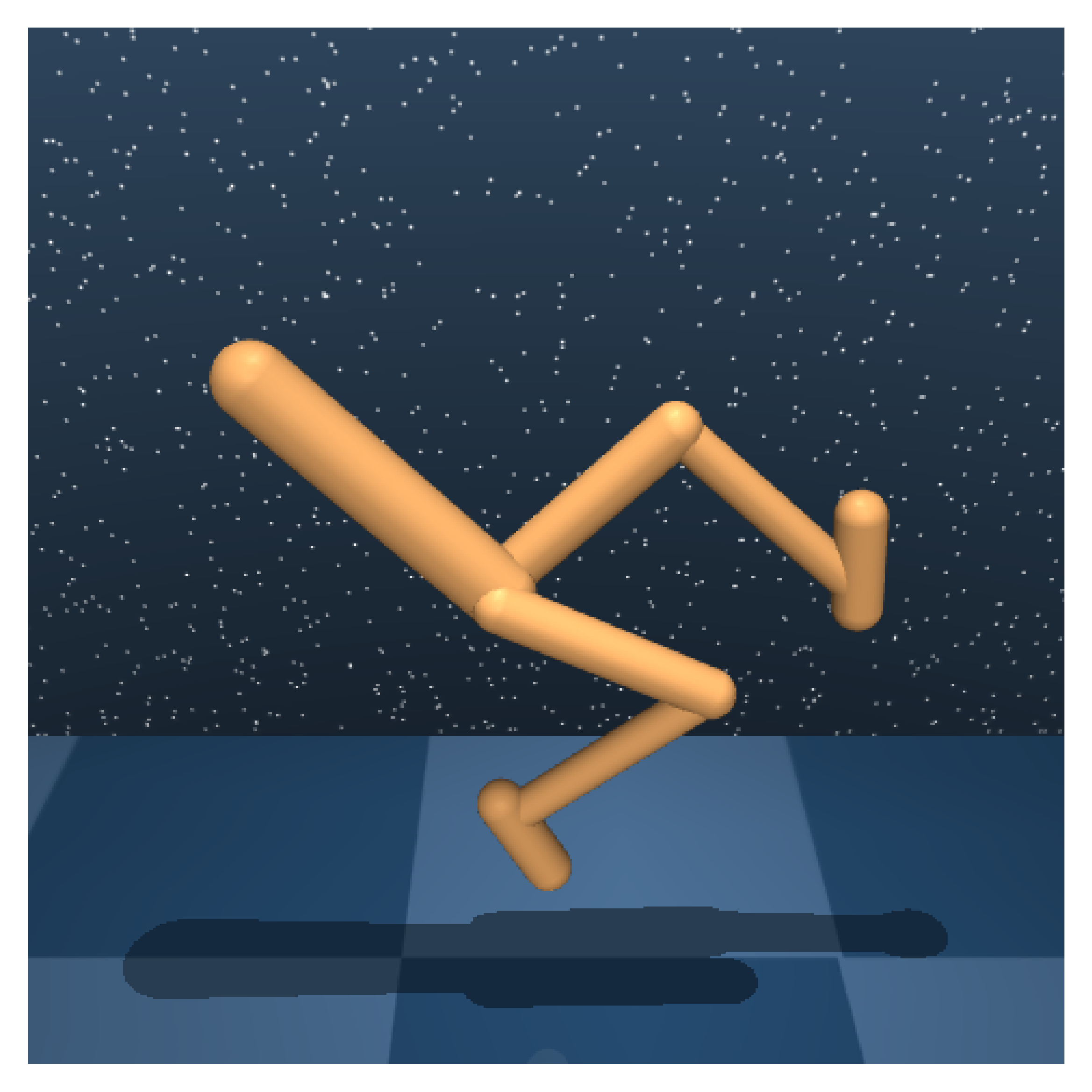
(f) walker_walk

Figure 8: Images for DMControl suites used in our experiments. Each image is a frame of a specific DMControl suite.

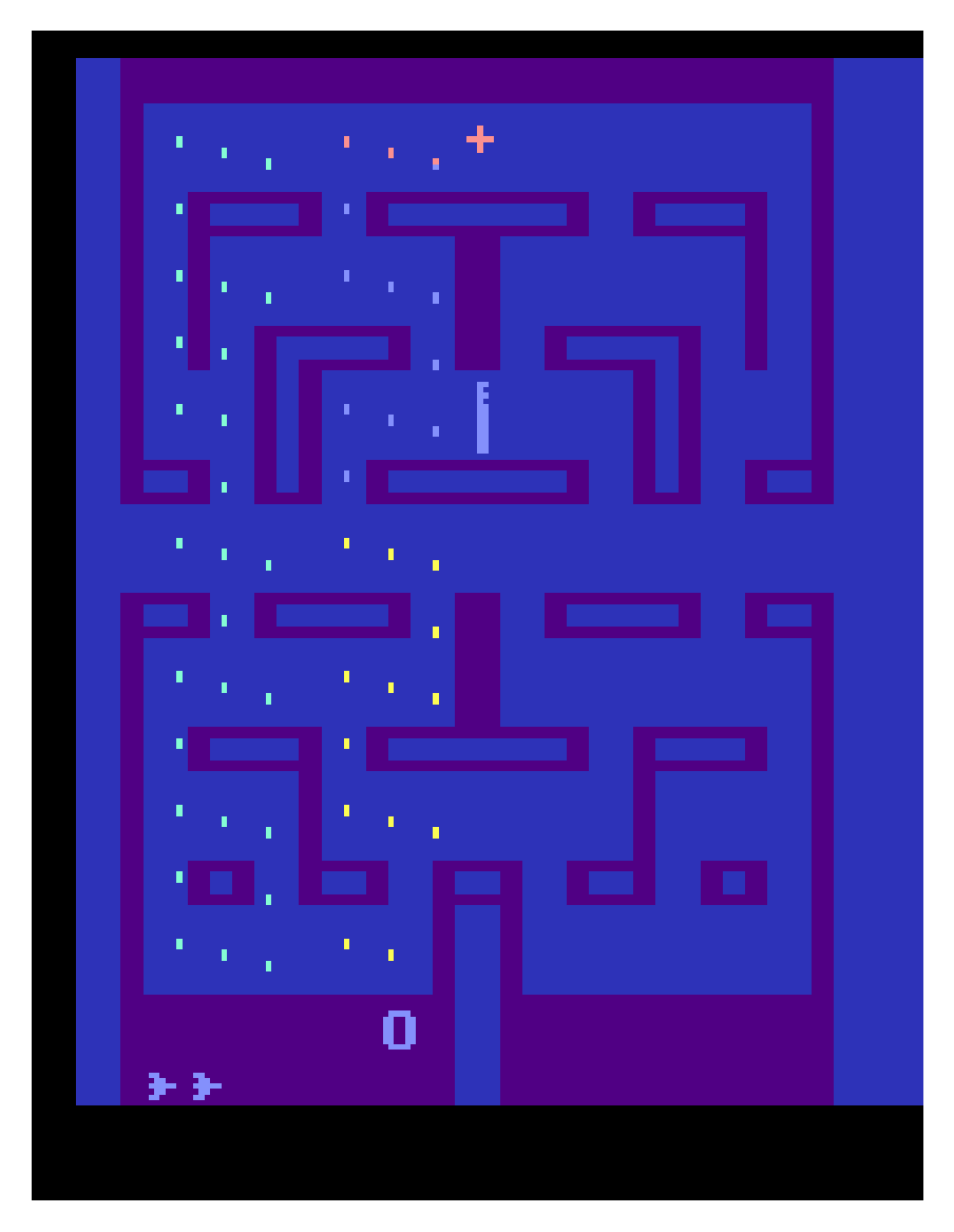
(a) Alien

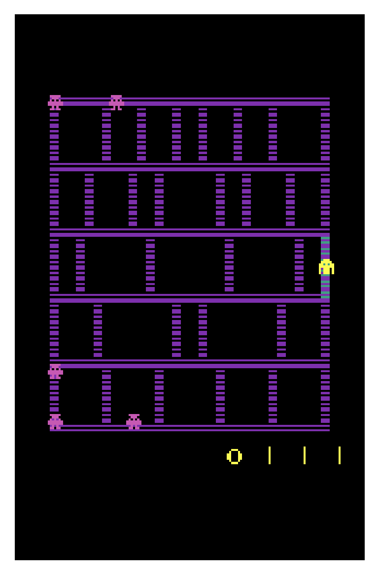
(b) Amidar

(c) Assault

(d) Asterix

(e) BankHeist

(f) BattleZone

(g) Boxing

(h) Breakout

(i) ChopperCommand

(j) CrazyClimber

(k) DemonAttack

(l) Freeway

(m) Frostbite

(n) Gopher

(o) Hero

(p) Jamesbond

Figure 9: Images for Atari100k suites used in our experiments. Each image is a frame of a specific Atari game.

(a) Kangaroo

(b) Krull

(c) KungFuMaster

(d) MsPacman

(e) Pong

(f) PrivateEye

(g) Qbert

(h) RoadRunner

(i) Seaquest

(j) UpNDown

Figure 10: Images for Atari100k suites used in our experiments (continuation of fig. 9). Each image is a frame of a specific Atari game.

Env	State Dimension	Action Dimension
InvertedPendulum	5	Continuous(1)
InvertedDoublePendulum	9	Continuous(1)
InvertedPendulumSwingup	5	Continuous(1)
Reacher	9	Continuous(2)
Walker2D	22	Continuous(6)
HalfCheetah	26	Continuous(6)
Ant	28	Continuous(8)
Hopper	15	Continuous(3)

Table 10: State dimension and action space for Bullet suite. Continuous($x$) means the action space is continuous with dimension $x$.

Env	State Dimension	Action Dimension
Reacher	11	Continuous(2)
Walker2d	17	Continuous(6)
HalfCheetah	17	Continuous(6)
Swimmer	8	Continuous(2)
Ant	111	Continuous(8)
Hopper	11	Continuous(3)
InvertedPendulum	4	Continuous(1)
InvertedDoublePendulum	11	Continuous(1)

Table 11: State space and action space for MuJoCo suite. Continuous($x$) means the action space is continuous with dimension $x$.

Domain	Tasks	State Space	Action Space
ball_in_cup	catch	(3, 100, 100)	Continuous(2)
cartpole	balance	(3, 100, 100)	Continuous(1)
cartpole	balance_sparse	(3, 100, 100)	Continuous(1)
cartpole	swingup	(3, 100, 100)	Continuous(1)
cartpole	swingup_sparse	(3, 100, 100)	Continuous(1)
cheetah	run	(3, 100, 100)	Continuous(6)
finger	spin	(3, 100, 100)	Continuous(2)
finger	turn_easy	(3, 100, 100)	Continuous(2)
finger	turn_hard	(3, 100, 100)	Continuous(2)
hopper	hop	(3, 100, 100)	Continuous(4)
hopper	stand	(3, 100, 100)	Continuous(4)
pendulum	swingup	(3, 100, 100)	Continuous(1)
reacher	easy	(3, 100, 100)	Continuous(2)
reacher	hard	(3, 100, 100)	Continuous(2)
walker	stand	(3, 100, 100)	Continuous(6)
walker	walk	(3, 100, 100)	Continuous(6)

Table 12: State space and action space for DMControl suite. Continuous($x$) means the action space is continuous with dimension $x$.

Game	State Space	Action Space
Alien	(210, 160, 3)	Discrete(18)
Amidar	(210, 160, 3)	Discrete(10)
Assault	(210, 160, 3)	Discrete(7)
Asterix	(210, 160, 3)	Discrete(9)
BankHeist	(210, 160, 3)	Discrete(18)
BattleZone	(210, 160, 3)	Discrete(18)
Boxing	(210, 160, 3)	Discrete(18)
Breakout	(210, 160, 3)	Discrete(4)
ChopperCommand	(210, 160, 3)	Discrete(18)
CrazyClimber	(210, 160, 3)	Discrete(9)
DemonAttack	(210, 160, 3)	Discrete(6)
Freeway	(210, 160, 3)	Discrete(3)
Frostbite	(210, 160, 3)	Discrete(18)
Gopher	(210, 160, 3)	Discrete(8)
Hero	(210, 160, 3)	Discrete(18)
Jamesbond	(210, 160, 3)	Discrete(18)
Kangaroo	(210, 160, 3)	Discrete(18)
Krull	(210, 160, 3)	Discrete(18)
KungFuMaster	(210, 160, 3)	Discrete(14)
MsPacman	(210, 160, 3)	Discrete(9)
Pong	(210, 160, 3)	Discrete(6)
PrivateEye	(210, 160, 3)	Discrete(18)
Qbert	(210, 160, 3)	Discrete(6)
RoadRunner	(210, 160, 3)	Discrete(18)
Seaquest	(210, 160, 3)	Discrete(18)
UpNDown	(210, 160, 3)	Discrete(6)

Table 13: State space and action space for Atari suite. Discrete($x$) means the action space is discrete with $x$ actions.

10 Appendix: Additional Experimental Results

In this section, we provide additional experimental results. PEER works by adding a regularization term to backbone DRL algorithms. Thus, the comparison with the backbone algorithm of PEER naturally becomes an ablation experiment. We provide more experiments to demonstrate the effectiveness of PEER.

10.1 Experiments on MuJoCo Suite

We present the performance of PEER on the MuJoCo suite in table 14. The results show that our proposed PEER outperforms or matches the compared algorithms in 5 out 7 MuJoCo environments. Compared with its backbone algorithm TD3, PEER surpasses it in 6 out of 7 environments.

Algorithm	Ant	HalfCheetah	Hopper	InvDouPen	InvPen	Reacher	Walker
PEER	​​5386 $\pm$493	10832 $\pm$ 501	​​3424 $\pm$180	7470 $\pm$ 3721	​​1000 $\pm$0	​​-4 $\pm$1	​​4223 $\pm$655
TD3	5102 $\pm$ 787	​​10858 $\pm$637	3163 $\pm$ 367	7312 $\pm$ 3653	1000 $\pm$ 0	-4 $\pm$ 1	3762 $\pm$ 956
METD3	2256 $\pm$ 431	5696 $\pm$ 1740	804 $\pm$ 71	7815 $\pm$ 0	912 $\pm$ 71	-8 $\pm$ 3	2079 $\pm$ 1096
SAC	4233 $\pm$ 806	10482 $\pm$ 959	2666 $\pm$ 320	​​9358 $\pm$0	1000 $\pm$ 0	-4 $\pm$ 0	4187 $\pm$ 304

Table 14: The average return of the last ten evaluations over ten random seeds. The maximum average returns are bolded. PEER outperforms or matches the other tested algorithms in 5 out of 7 environments.

In table 15, we show comparisons with model-free algorithm REDQ [62] on pybullet suite.

Algo	Ant	Hopper	Walker
PEER	​​5386 $\pm$ 493	​​3424 $\pm$ 180	​​4223 $\pm$ 655
REDQ	3900 $\pm$ 890	2656 $\pm$ 759	4211 $\pm$ 524

Table 15: Average return for PEER and REDQ. PEER surpasses REDQ on all tested tasks. The REDQ results are obtained using the authors’ implementation and are reported over 20 trials.

10.2 Combination with Model-based Algorithm

In table 16, we show comparisons with model-based methods algorithms TDMPC and Dreamer-v2 on DMControl suites. In table 17, we show comparisons with model-based algorithms Dreamer-v2. Note that the data we take directly from the authors’ dreamer-v2 codebase (https://github.com/danijar/dreamerv2/tree/main/scores), the amount of data they use is 1000k, which is 10 times more than our PEER. The PEER scores in table 17 are taken as the largest of PEER+DrQ and PEER+CURL.

500K Step Scores	Finger, Spin	Cartpole, Swingup	Reacher, Easy	Cheetah, run	Walker, Walk	Ball_in_cup, Catch
PEER + CURL	​​864 $\pm$ 160	​​866 $\pm$ 17	​​980 $\pm$ 3	​​732 $\pm$ 41	​​946 $\pm$ 17	​​971 $\pm$ 5
Dreamer-V2	386 $\pm$ 83	853 $\pm$ 15	876 $\pm$ 60	610 $\pm$ 117	934 $\pm$ 16	792 $\pm$300
100K Step Scores
PRER +TDMPC	772 $\pm$ 107	​​848 $\pm$ 25	​​841 $\pm$ 115	​​636 $\pm$ 35	​​876 $\pm$ 41	​​937 $\pm$ 96
TDMPC	​​943 $\pm$ 59	770 $\pm$ 70	628 $\pm$ 105	222 $\pm$ 88	577 $\pm$ 208	933 $\pm$ 24
Dreamer-V2	414 $\pm$ 93	697 $\pm$ 176	633 $\pm$ 248	501 $\pm$ 146	705 $\pm$ 232	693 $\pm$335

Table 16: Comparison with model-based methods. PEER outperforms Dreamer-v2 on 12 out of 12 tasks. PEER (combined with TDMPC [63]) outperforms TDMPC by on 5 out of 6 tasks.

Game	PEER	Dreamer-V2	MuZero
Alien	​​1218.9	384.1	530.0
Amidar	​​185.2	29.8	38.8
Assault	​​721.0	433.4	500.1
Asterix	918.2	330.6	​​1734.0
BHeist	78.6	127.1	​​192.5
BZone	​​15727.3	4200.0	7687.5
Boxing	14.5	​​37.7	15.1
Breakout	8.5	1.5	​​48.0
ChpCmd	​​1451.8	687.5	1350.0
CzClmr	18922.7	25232.5	​​56937.0
DmAttack	1236.7	182.9	​​3527.0
Freeway	​​30.4	11.6	21.8
Frostbite	​​2151.0	302.5	255.0
Gopher	681.8	820.2	​​1256.0
Hero	​​7499.9	2185.0	3095.0
Jbond	​​414.1	81.2	87.5
Kangaroo	​​1148.2	150.0	62.5
Krull	​​5444.7	3853.8	4890.8
KFMaster	15439.1	12420.3	​​18813.0
MsPacman	​​1768.4	647.9	1265.6
Pong	-9.5	-18.3	​​-6.7
PriEye	​​3207.7	188.8	56.3
Qbert	2197.7	318.6	​​3952.0
RdRunner	​​10697.3	3622.5	2500.0
Squest	​​538.5	356.0	208.0
UpNDown	7680.9	​​8025.1	2896.9

Table 17: PEER outperforms Dreamer-v2 and Muzero on 21 and 16 games of Atari26 where Dreamer-v2 even uses 10 times the data of PEER. Note that the data we take directly from the authors’ dreamer-v2 codebase, the amount of data for Dreamer-V2 they use is 1000k, which is 10 times more than our PEER.

10.3 Various $\beta$ for Performance Improvement

Fine-tuning for hyper-parameters probably improves the performance of PEER. To see this, we select 7 Atari environments to investigate the effect of fine-tuning $\beta$, where PEER (coupled with CURL) achieves SOTA performance. We present the results in fig. 11. There is no one value taken that is significantly better than the other. We see that large $\beta$ (=1e-2) may result in the failure of learning (on Freeway game) but may also bring the best performance improvements (on Kangaroo game). Overall, fine-tuning the hyper-parameter $\beta$ may improve the empirical performance by a large margin.

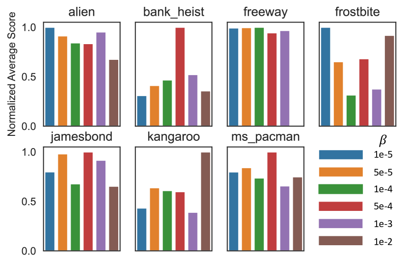
Figure 11: The average scores normalized by the max average score on the 7 Atari games for selected 6 hyper-parameter $\beta$. From the experiments, we can see that fine-tuning the $\beta$ may result in performance improvements.

10.4 Performance curves on DMControl Tasks

We present the performance curves of PEER on a total of 16 DMControl environments in fig. 12 and fig. 13. We run 10 seeds in each environment.

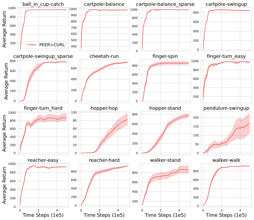
Figure 12: Performance curves for PEER (coupled with CURL) on DMControl suite. The shaded region represents half the standard deviation of the average evaluation over 10 seeds. The curves are smoothed by moving average.

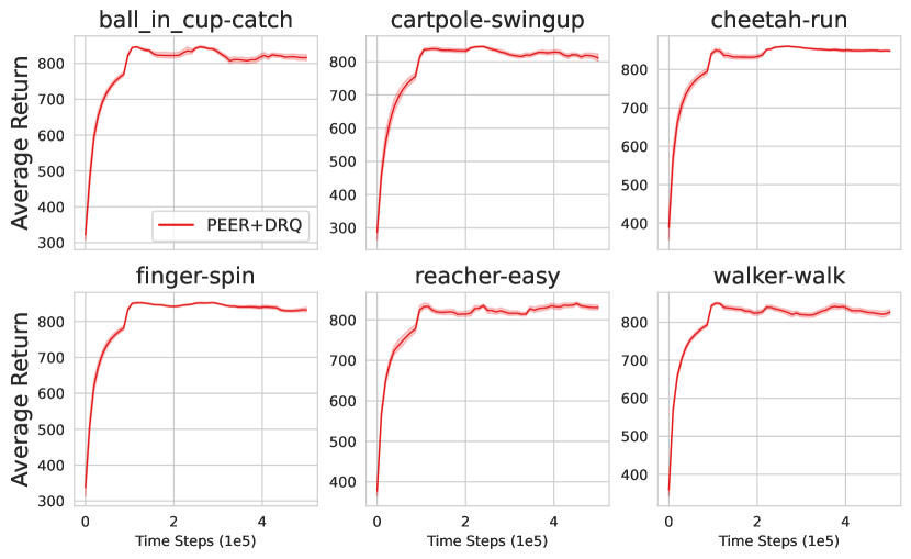
Figure 13: Performance curves for PEER (coupled with DrQ) on DMControl suite. The shaded region represents half the standard deviation of the average evaluation over 10 seeds. The curves are smoothed by moving average.

References

- Silver et al. [2018] David Silver, Thomas Hubert, Julian Schrittwieser, Ioannis Antonoglou, Matthew Lai, Arthur Guez, Marc Lanctot, Laurent Sifre, Dharshan Kumaran, Thore Graepel, et al. A general reinforcement learning algorithm that masters chess, shogi, and go through self-play. Science, 362(6419):1140–1144, 2018.
- Mnih et al. [2015] Volodymyr Mnih, Koray Kavukcuoglu, David Silver, Andrei A Rusu, Joel Veness, Marc G Bellemare, Alex Graves, Martin Riedmiller, Andreas K Fidjeland, Georg Ostrovski, et al. Human-level control through deep reinforcement learning. nature, 518(7540):529–533, 2015.
- Vinyals et al. [2019] Oriol Vinyals, Igor Babuschkin, Wojciech M Czarnecki, Michaël Mathieu, Andrew Dudzik, Junyoung Chung, David H Choi, Richard Powell, Timo Ewalds, Petko Georgiev, et al. Grandmaster level in starcraft ii using multi-agent reinforcement learning. Nature, 575(7782):350–354, 2019.
- Haarnoja et al. [2018] Tuomas Haarnoja, Aurick Zhou, Pieter Abbeel, and Sergey Levine. Soft actor-critic: Off-policy maximum entropy deep reinforcement learning with a stochastic actor. In International conference on machine learning, pages 1861–1870. PMLR, 2018.
- Hafner et al. [2019] Danijar Hafner, Timothy P. Lillicrap, Ian Fischer, Ruben Villegas, David Ha, Honglak Lee, and James Davidson. Learning latent dynamics for planning from pixels. In Kamalika Chaudhuri and Ruslan Salakhutdinov, editors, Proceedings of the 36th International Conference on Machine Learning, ICML 2019, 9-15 June 2019, Long Beach, California, USA, volume 97 of Proceedings of Machine Learning Research, pages 2555–2565. PMLR, 2019. URL http://proceedings.mlr.press/v97/hafner19a.html.
- Laskin et al. [2020a] Michael Laskin, Aravind Srinivas, and Pieter Abbeel. Curl: Contrastive unsupervised representations for reinforcement learning. In International Conference on Machine Learning, pages 5639–5650. PMLR, 2020a.
- Hafner et al. [2020] Danijar Hafner, Timothy P. Lillicrap, Jimmy Ba, and Mohammad Norouzi. Dream to control: Learning behaviors by latent imagination. In 8th International Conference on Learning Representations, ICLR 2020, Addis Ababa, Ethiopia, April 26-30, 2020. OpenReview.net, 2020. URL https://openreview.net/forum?id=S1lOTC4tDS.
- Yarats et al. [2021a] Denis Yarats, Amy Zhang, Ilya Kostrikov, Brandon Amos, Joelle Pineau, and Rob Fergus. Improving sample efficiency in model-free reinforcement learning from images. In Thirty-Fifth AAAI Conference on Artificial Intelligence, AAAI 2021, Thirty-Third Conference on Innovative Applications of Artificial Intelligence, IAAI 2021, The Eleventh Symposium on Educational Advances in Artificial Intelligence, EAAI 2021, Virtual Event, February 2-9, 2021, pages 10674–10681. AAAI Press, 2021a. URL https://ojs.aaai.org/index.php/AAAI/article/view/17276.
- Yarats et al. [2021b] Denis Yarats, Ilya Kostrikov, and Rob Fergus. Image augmentation is all you need: Regularizing deep reinforcement learning from pixels. In 9th International Conference on Learning Representations, ICLR 2021, Virtual Event, Austria, May 3-7, 2021. OpenReview.net, 2021b. URL https://openreview.net/forum?id=GY6-6sTvGaf.
- Chen et al. [2021] Lili Chen, Kevin Lu, Aravind Rajeswaran, Kimin Lee, Aditya Grover, Michael Laskin, Pieter Abbeel, Aravind Srinivas, and Igor Mordatch. Decision transformer: Reinforcement learning via sequence modeling. In Marc’Aurelio Ranzato, Alina Beygelzimer, Yann N. Dauphin, Percy Liang, and Jennifer Wortman Vaughan, editors, Advances in Neural Information Processing Systems 34: Annual Conference on Neural Information Processing Systems 2021, NeurIPS 2021, December 6-14, 2021, virtual, pages 15084–15097, 2021. URL https://proceedings.neurips.cc/paper/2021/hash/7f489f642a0ddb10272b5c31057f0663-Abstract.html.
- Janner et al. [2021] Michael Janner, Qiyang Li, and Sergey Levine. Offline reinforcement learning as one big sequence modeling problem. In Marc’Aurelio Ranzato, Alina Beygelzimer, Yann N. Dauphin, Percy Liang, and Jennifer Wortman Vaughan, editors, Advances in Neural Information Processing Systems 34: Annual Conference on Neural Information Processing Systems 2021, NeurIPS 2021, December 6-14, 2021, virtual, pages 1273–1286, 2021. URL https://proceedings.neurips.cc/paper/2021/hash/099fe6b0b444c23836c4a5d07346082b-Abstract.html.
- Schmidhuber [1990] Jiirgen Schmidhuber. Making the world differentiable: On using self-supervised fully recurrent neural networks for dynamic reinforcement learning and planning in non-stationary environments. Technical Report, 1990.
- Jaderberg et al. [2017] Max Jaderberg, Volodymyr Mnih, Wojciech Marian Czarnecki, Tom Schaul, Joel Z. Leibo, David Silver, and Koray Kavukcuoglu. Reinforcement learning with unsupervised auxiliary tasks. In 5th International Conference on Learning Representations, ICLR 2017, Toulon, France, April 24-26, 2017, Conference Track Proceedings. OpenReview.net, 2017. URL https://openreview.net/forum?id=SJ6yPD5xg.
- Jaderberg et al. [2016] Max Jaderberg, Volodymyr Mnih, Wojciech Marian Czarnecki, Tom Schaul, Joel Z Leibo, David Silver, and Koray Kavukcuoglu. Reinforcement learning with unsupervised auxiliary tasks. arXiv preprint arXiv:1611.05397, 2016.
- Guo et al. [2020] Zhaohan Daniel Guo, Bernardo Avila Pires, Bilal Piot, Jean-Bastien Grill, Florent Altché, Rémi Munos, and Mohammad Gheshlaghi Azar. Bootstrap latent-predictive representations for multitask reinforcement learning. In International Conference on Machine Learning, pages 3875–3886. PMLR, 2020.
- Oord et al. [2018] Aaron van den Oord, Yazhe Li, and Oriol Vinyals. Representation learning with contrastive predictive coding. arXiv preprint arXiv:1807.03748, 2018.
- Lyle et al. [2021a] Clare Lyle, Mark Rowland, Georg Ostrovski, and Will Dabney. On the effect of auxiliary tasks on representation dynamics. In International Conference on Artificial Intelligence and Statistics, pages 1–9. PMLR, 2021a.
- Yarats et al. [2021c] Denis Yarats, Ilya Kostrikov, and Rob Fergus. Image augmentation is all you need: Regularizing deep reinforcement learning from pixels. In International Conference on Learning Representations, 2021c. URL https://openreview.net/forum?id=GY6-6sTvGaf.
- Ghosh and Bellemare [2020] Dibya Ghosh and Marc G Bellemare. Representations for stable off-policy reinforcement learning. In International Conference on Machine Learning, pages 3556–3565. PMLR, 2020.
- Laskin et al. [2020b] Michael Laskin, Kimin Lee, Adam Stooke, Lerrel Pinto, Pieter Abbeel, and Aravind Srinivas. Reinforcement learning with augmented data. In Hugo Larochelle, Marc’Aurelio Ranzato, Raia Hadsell, Maria-Florina Balcan, and Hsuan-Tien Lin, editors, Advances in Neural Information Processing Systems 33: Annual Conference on Neural Information Processing Systems 2020, NeurIPS 2020, December 6-12, 2020, virtual, 2020b. URL https://proceedings.neurips.cc/paper/2020/hash/e615c82aba461681ade82da2da38004a-Abstract.html.
- Bellemare et al. [2019a] Marc Bellemare, Will Dabney, Robert Dadashi, Adrien Ali Taiga, Pablo Samuel Castro, Nicolas Le Roux, Dale Schuurmans, Tor Lattimore, and Clare Lyle. A geometric perspective on optimal representations for reinforcement learning. Advances in neural information processing systems, 32, 2019a.
- Dadashi et al. [2019] Robert Dadashi, Adrien Ali Taiga, Nicolas Le Roux, Dale Schuurmans, and Marc G Bellemare. The value function polytope in reinforcement learning. In International Conference on Machine Learning, pages 1486–1495. PMLR, 2019.
- Eysenbach et al. [2021] Benjamin Eysenbach, Ruslan Salakhutdinov, and Sergey Levine. The information geometry of unsupervised reinforcement learning. arXiv preprint arXiv:2110.02719, 2021.
- Lyle et al. [2021b] Clare Lyle, Mark Rowland, and Will Dabney. Understanding and preventing capacity loss in reinforcement learning. In Deep RL Workshop NeurIPS 2021, 2021b.
- Levine et al. [2017] Nir Levine, Tom Zahavy, Daniel J. Mankowitz, Aviv Tamar, and Shie Mannor. Shallow updates for deep reinforcement learning. In Isabelle Guyon, Ulrike von Luxburg, Samy Bengio, Hanna M. Wallach, Rob Fergus, S. V. N. Vishwanathan, and Roman Garnett, editors, Advances in Neural Information Processing Systems 30: Annual Conference on Neural Information Processing Systems 2017, December 4-9, 2017, Long Beach, CA, USA, pages 3135–3145, 2017. URL https://proceedings.neurips.cc/paper/2017/hash/393c55aea738548df743a186d15f3bef-Abstract.html.
- Dabney et al. [2021] Will Dabney, André Barreto, Mark Rowland, Robert Dadashi, John Quan, Marc G. Bellemare, and David Silver. The value-improvement path: Towards better representations for reinforcement learning. In Thirty-Fifth AAAI Conference on Artificial Intelligence, AAAI 2021, Thirty-Third Conference on Innovative Applications of Artificial Intelligence, IAAI 2021, The Eleventh Symposium on Educational Advances in Artificial Intelligence, EAAI 2021, Virtual Event, February 2-9, 2021, pages 7160–7168. AAAI Press, 2021. URL https://ojs.aaai.org/index.php/AAAI/article/view/16880.
- Sutton and Barto [2018] Richard S Sutton and Andrew G Barto. Reinforcement learning: An introduction. MIT press, 2018.
- Fujimoto et al. [2018] Scott Fujimoto, Herke Hoof, and David Meger. Addressing function approximation error in actor-critic methods. In International Conference on Machine Learning, pages 1587–1596. PMLR, 2018.
- Coumans and Bai [2016–2021] Erwin Coumans and Yunfei Bai. Pybullet, a python module for physics simulation for games, robotics and machine learning. http://pybullet.org, 2016–2021.
- Tunyasuvunakool et al. [2020] Saran Tunyasuvunakool, Alistair Muldal, Yotam Doron, Siqi Liu, Steven Bohez, Josh Merel, Tom Erez, Timothy Lillicrap, Nicolas Heess, and Yuval Tassa. dm-control: Software and tasks for continuous control. Software Impacts, 6:100022, 2020. ISSN 2665-9638. doi: https://doi.org/10.1016/j.simpa.2020.100022. URL https://www.sciencedirect.com/science/article/pii/S2665963820300099.
- Todorov et al. [2012] Emanuel Todorov, Tom Erez, and Yuval Tassa. Mujoco: A physics engine for model-based control. In 2012 IEEE/RSJ International Conference on Intelligent Robots and Systems, IROS 2012, Vilamoura, Algarve, Portugal, October 7-12, 2012, pages 5026–5033. IEEE, 2012. doi: 10.1109/IROS.2012.6386109. URL https://doi.org/10.1109/IROS.2012.6386109.
- Bellemare et al. [2013] M. G. Bellemare, Y. Naddaf, J. Veness, and M. Bowling. The arcade learning environment: An evaluation platform for general agents. Journal of Artificial Intelligence Research, 47:253–279, jun 2013.
- Boyan [1999] Justin A. Boyan. Least-squares temporal difference learning. In Ivan Bratko and Saso Dzeroski, editors, Proceedings of the Sixteenth International Conference on Machine Learning (ICML 1999), Bled, Slovenia, June 27 - 30, 1999, pages 49–56. Morgan Kaufmann, 1999.
- Bellemare et al. [2019b] Marc G. Bellemare, Will Dabney, Robert Dadashi, Adrien Ali Taïga, Pablo Samuel Castro, Nicolas Le Roux, Dale Schuurmans, Tor Lattimore, and Clare Lyle. A geometric perspective on optimal representations for reinforcement learning. In Hanna M. Wallach, Hugo Larochelle, Alina Beygelzimer, Florence d’Alché-Buc, Emily B. Fox, and Roman Garnett, editors, Advances in Neural Information Processing Systems 32: Annual Conference on Neural Information Processing Systems 2019, NeurIPS 2019, December 8-14, 2019, Vancouver, BC, Canada, pages 4360–4371, 2019b. URL https://proceedings.neurips.cc/paper/2019/hash/3cf2559725a9fdfa602ec8c887440f32-Abstract.html.
- Lillicrap et al. [2016] Timothy P Lillicrap, Jonathan J Hunt, Alexander Pritzel, Nicolas Heess, Tom Erez, Yuval Tassa, David Silver, and Daan Wierstra. Continuous control with deep reinforcement learning. In ICLR (Poster), 2016.
- Rudolf [2018] Daniel Rudolf. An upper bound of the minimal dispersion via delta covers. In Contemporary Computational Mathematics-A Celebration of the 80th Birthday of Ian Sloan, pages 1099–1108. Springer, 2018.
- Andrychowicz et al. [2021] Marcin Andrychowicz, Anton Raichuk, Piotr Stańczyk, Manu Orsini, Sertan Girgin, Raphaël Marinier, Léonard Hussenot, Matthieu Geist, Olivier Pietquin, Marcin Michalski, et al. What matters in on-policy reinforcement learning? a large-scale empirical study. In ICLR 2021-Ninth International Conference on Learning Representations, 2021.
- Henderson et al. [2018] Peter Henderson, Riashat Islam, Philip Bachman, Joelle Pineau, Doina Precup, and David Meger. Deep reinforcement learning that matters. In Thirty-Second AAAI Conference on Artificial Intelligence, 2018.
- Brockman et al. [2016] Greg Brockman, Vicki Cheung, Ludwig Pettersson, Jonas Schneider, John Schulman, Jie Tang, and Wojciech Zaremba. Openai gym, 2016.
- Schulman et al. [2015] John Schulman, Sergey Levine, Pieter Abbeel, Michael Jordan, and Philipp Moritz. Trust region policy optimization. In International conference on machine learning, pages 1889–1897, 2015.
- Schulman et al. [2017] John Schulman, Filip Wolski, Prafulla Dhariwal, Alec Radford, and Oleg Klimov. Proximal policy optimization algorithms. arXiv preprint arXiv:1707.06347, 2017.
- He et al. [2021] Qiang He, Chen Gong, Yuxun Qu, Xiaoyu Chen, Xinwen Hou, and Yu Liu. Mepg: A minimalist ensemble policy gradient framework for deep reinforcement learning. arXiv preprint arXiv:2109.10552, 2021.
- Warde-Farley et al. [2013] David Warde-Farley, Ian J. Goodfellow, Aaron Courville, and Yoshua Bengio. An empirical analysis of dropout in piecewise linear networks. 2013.
- Srivastava et al. [2014] Nitish Srivastava, Geoffrey Hinton, Alex Krizhevsky, Ilya Sutskever, and Ruslan Salakhutdinov. Dropout: a simple way to prevent neural networks from overfitting. The journal of machine learning research, 15(1):1929–1958, 2014.
- Yarats and Kostrikov [2020] Denis Yarats and Ilya Kostrikov. Soft actor-critic (sac) implementation in pytorch. https://github.com/denisyarats/pytorch_sac, 2020.
- Dhariwal et al. [2017] Prafulla Dhariwal, Christopher Hesse, Oleg Klimov, Alex Nichol, Matthias Plappert, Alec Radford, John Schulman, Szymon Sidor, Yuhuai Wu, and Peter Zhokhov. Openai baselines. https://github.com/openai/baselines, 2017.
- Doersch [2016] Carl Doersch. Tutorial on variational autoencoders. arXiv preprint arXiv:1606.05908, 2016.
- Kielak [2020] Kacper Piotr Kielak. Do recent advancements in model-based deep reinforcement learning really improve data efficiency? In URL https://openreview. net/forum, page 6, 2020.
- van Hasselt et al. [2019] Hado van Hasselt, Matteo Hessel, and John Aslanides. When to use parametric models in reinforcement learning? In Hanna M. Wallach, Hugo Larochelle, Alina Beygelzimer, Florence d’Alché-Buc, Emily B. Fox, and Roman Garnett, editors, Advances in Neural Information Processing Systems 32: Annual Conference on Neural Information Processing Systems 2019, NeurIPS 2019, December 8-14, 2019, Vancouver, BC, Canada, pages 14322–14333, 2019. URL https://proceedings.neurips.cc/paper/2019/hash/1b742ae215adf18b75449c6e272fd92d-Abstract.html.
- Devlin et al. [2019] Jacob Devlin, Ming-Wei Chang, Kenton Lee, and Kristina Toutanova. BERT: pre-training of deep bidirectional transformers for language understanding. In Jill Burstein, Christy Doran, and Thamar Solorio, editors, Proceedings of the 2019 Conference of the North American Chapter of the Association for Computational Linguistics: Human Language Technologies, NAACL-HLT 2019, Minneapolis, MN, USA, June 2-7, 2019, Volume 1 (Long and Short Papers), pages 4171–4186. Association for Computational Linguistics, 2019. doi: 10.18653/v1/n19-1423. URL https://doi.org/10.18653/v1/n19-1423.
- He et al. [2020] Kaiming He, Haoqi Fan, Yuxin Wu, Saining Xie, and Ross Girshick. Momentum contrast for unsupervised visual representation learning. In Proceedings of the IEEE/CVF conference on computer vision and pattern recognition, pages 9729–9738, 2020.
- Chen et al. [2020a] Xinlei Chen, Haoqi Fan, Ross Girshick, and Kaiming He. Improved baselines with momentum contrastive learning. arXiv preprint arXiv:2003.04297, 2020a.
- Chen et al. [2020b] Ting Chen, Simon Kornblith, Mohammad Norouzi, and Geoffrey E. Hinton. A simple framework for contrastive learning of visual representations. In Proceedings of the 37th International Conference on Machine Learning, ICML 2020, 13-18 July 2020, Virtual Event, volume 119 of Proceedings of Machine Learning Research, pages 1597–1607. PMLR, 2020b. URL http://proceedings.mlr.press/v119/chen20j.html.
- Hénaff [2020] Olivier J. Hénaff. Data-efficient image recognition with contrastive predictive coding. In Proceedings of the 37th International Conference on Machine Learning, ICML 2020, 13-18 July 2020, Virtual Event, volume 119 of Proceedings of Machine Learning Research, pages 4182–4192. PMLR, 2020. URL http://proceedings.mlr.press/v119/henaff20a.html.
- Van Hasselt et al. [2016] Hado Van Hasselt, Arthur Guez, and David Silver. Deep reinforcement learning with double q-learning. In Thirtieth AAAI conference on artificial intelligence, 2016.
- Bellemare et al. [2017] Marc G Bellemare, Will Dabney, and Rémi Munos. A distributional perspective on reinforcement learning. arXiv preprint arXiv:1707.06887, 2017.
- He and Hou [2020] Qiang He and Xinwen Hou. Wd3: Taming the estimation bias in deep reinforcement learning. In 2020 IEEE 32nd International Conference on Tools with Artificial Intelligence (ICTAI), pages 391–398. IEEE, 2020.
- Kumar et al. [2021] Aviral Kumar, Rishabh Agarwal, Tengyu Ma, Aaron Courville, George Tucker, and Sergey Levine. Dr3: Value-based deep reinforcement learning requires explicit regularization. In International Conference on Learning Representations, 2021.
- Vershynin [2010] Roman Vershynin. Introduction to the non-asymptotic analysis of random matrices. arXiv preprint arXiv:1011.3027, 2010.
- Raffin et al. [2021] Antonin Raffin, Ashley Hill, Adam Gleave, Anssi Kanervisto, Maximilian Ernestus, and Noah Dormann. Stable-baselines3: Reliable reinforcement learning implementations. Journal of Machine Learning Research, 22(268):1–8, 2021. URL http://jmlr.org/papers/v22/20-1364.html.
- Kingma and Ba [2015] Diederik P Kingma and Jimmy Ba. Adam: A method for stochastic optimization. In ICLR (Poster), 2015.
- Chen et al. [2020c] Xinyue Chen, Che Wang, Zijian Zhou, and Keith W Ross. Randomized ensembled double q-learning: Learning fast without a model. In International Conference on Learning Representations, 2020c.
- Hansen et al. [2022] Nicklas Hansen, Hao Su, and Xiaolong Wang. Temporal difference learning for model predictive control. In Kamalika Chaudhuri, Stefanie Jegelka, Le Song, Csaba Szepesvári, Gang Niu, and Sivan Sabato, editors, International Conference on Machine Learning, ICML 2022, 17-23 July 2022, Baltimore, Maryland, USA, volume 162 of Proceedings of Machine Learning Research, pages 8387–8406. PMLR, 2022. URL https://proceedings.mlr.press/v162/hansen22a.html.