Configurational microcanonical statistical mechanics from Riemannian geometry of equipotenital level sets

Abstract

In the present work, we present a detailed discussion of a Riemannian metric structure originally introduced in [Gori et al., J. Stat. Mech., 9 093204 (2018)] on the configuration space and on phase space allowing to interpret the derivatives of the configurational microcanonical entropy and of the canonical entropy in terms of integrals of extrinsic geoemtrical quantities associated to the equipotential level sets.

I Introduction

In the last decades, a field of research has been established aiming at investigating how thermodynamic properties of classical systems arise from the geometrical properties of the equipotential level sets in configuration spacePettini (2007); Franzosi (2011). For instance, the so-called Topological Theory (TT) on the origin of phase transitions (PT) in classical systems, developed in the last three decades, represents one of the conceptual frameworks that have contributed to orienting the research in this field and have provided a generalization of the statistical mechanical description of phase transitions in small or mesoscopic systems. According to TT, the singularities of thermodynamic potentials - arising in the thermodynamic limit in the canonical and grancanonical ensembles - would be induced by suitable topological changes of some submanifolds of configuration space. These same topological changes can occur for any finite number of degrees of freedom. This theory, supported by many pieces of evidence ranging from numerical simulations to exact analytic computations carried on different statistical models have been rigorously rooted in two theorems that associate topological changes of the equipotential level sets of configuration space with the loss of analyticity of microcanonical configuration entropy. In particular, one of these theorems named Necessity theorem, states that in its original formulation that if all the equipotential level sets in a certain interval of specific potential energy $\displaystyle[\bar{v}_{1},\bar{v}_{2}]$ are diffeomorphic among them at any finite, then the system cannot undergo any phase transition in the corresponding interval of temperatures for short-range regular potential. According to Morse Theory, this statement can be rephrased as follows: the absence of critical points of the potential energy in the specific potential energy $\displaystyle[\bar{v}_{1},\bar{v}_{2}]$ at any finite N implies the absence of phase transition in the corresponding interval of temperatures. In the last decade, a counterexample to the original formulation of the Necessity Theorem has been found: for the $\displaystyle\phi^{4}$ model on a 2D lattice and nearest neighbors interactions, there are no critical points of the potential energy for the critical value of the specific potential energy $\displaystyle\bar{v}_{c}$ corresponding to the second-order phase transition observed at the critical temperature $\displaystyle T_{c}$ in the thermodynamic limit. These findings oriented the research towards a refinement of the topological theory leading to a new formulation of the Necessity Theorem including the hypothesis of asymptotic diffeomorphicity of equipotential level sets in thermodynamic limit. In the conceptualization process leading to such a development of the Topological Theory (TT), it appears to be a key step to search for a clear connection between the Riemannian geometric properties of the regular equipotential level sets and the derivatives of the configurational microcanonical entropy with respect to specific potential energy. The natural kinetic energy metric in configuration space does not provide a suited framework for this purpose.
In the present work, we present a method to define a Riemannian metric structure both in configuration space in the absence of critical points of potential energy allowing to provide clear identification of the derivatives of the configurational microcanonical entropy with integrals of extrinsic geometric curvature over equipotential (isoenergetic) level sets.

II Geometry of regular potential energy level sets in configuration space

II.1 Microcanonical configurational statistical mechanics from differential topology of regular equipotential level sets

We consider in what follows the configurational microcanonical ensemble $\displaystyle(\Lambda_{q},\rho_{N}(\mathbf{q};\overline{v}))$ where the constraint is obtained by fixing the value of some specific potential energy function $\displaystyle\overline{V}_{N}:\Lambda_{q}\longrightarrow\mathbb{R}$ and the corresponding microcanonical configurational density function is given by

$$\rho_{N}(\mathbf{q};\overline{v})=\dfrac{\delta\left(\overline{V}_{N}(\mathbf{q})-\overline{v}\right)}{\int_{\mathcal{X}^{N}}\delta\left(\overline{V}_{N}(\mathbf{q})-\overline{v}\right)\mathrm{d}\mathrm{Vol}_{g}}.$$ (1)

where $\displaystyle g$ is a natural metric structure in configuration space and $\displaystyle\mathrm{d}\mathrm{Vol}_{g}$ the associated Riemannian volume form. The normalization constant in (1) is the microcanonical partition function according to Boltzmann’s definition:

$$\Omega_{N,\mathrm{Boltz}}(\overline{v})=\dfrac{\partial}{\partial\overline{v}}\Omega_{N,\mathrm{Gibbs}}(\overline{v})=\dfrac{\partial}{\partial\overline{v}}\int_{\Lambda_{q}}\Theta(\overline{V}_{N}(\mathbf{q})-\overline{v})\mathrm{d}\mathrm{Vol}_{g}=\int_{\Lambda_{q}}\delta\left(\overline{V}_{N}(\mathbf{q})-\overline{v}\right)\mathrm{d}\mathrm{Vol}_{g}$$ (2)

where $\displaystyle\Theta(x)$ is the Heaviside step function.
In analogy with the usual definitions in statistical microcanonical ensemble, the configurational microcanonical entropy density function is given by:

$$\overline{S}_{N,\mathrm{Boltz}}=\dfrac{1}{N}\ln\Omega_{N,\mathrm{Boltz}}(\overline{v})$$ (3)

As a consequence of eq.(3), the microcanonical volume of the level sets of $\displaystyle\overline{V}_{N}$ as a function of $\displaystyle\bar{v}$ contains the whole information on the thermodynamics of the system.
In what follows, the thermodynamic properties of the configurational microcanonical ensemble are expressed as integrals of quantities associated with the vector field that generates the diffeomorphism among the level sets of $\displaystyle\overline{V}_{N}$.

Definition II.1 (Equipotential level sets).

We recall that the equipotential level sets $\displaystyle\Sigma_{\bar{v}}^{\overline{V}_{N}}$ are defined as

$$\Sigma_{\bar{v}}^{\overline{V}_{N}}=\left\{q\in\Lambda_{q}|\overline{V}_{N}(q)=\overline{v}\right\}$$ (4)

Remark 1 (Compactness of level sets).

As $\displaystyle\overline{V}_{N}\in C^{\infty}(\Lambda_{q})$ is a continuous function then $\displaystyle\overline{V}_{N}^{-1}(\overline{v})\subseteq\Lambda_{q}$ is a compact set.

Let the gradient vector field $\displaystyle\boldsymbol{\mathrm{grad}}_{g}\overline{V}_{N}\in\mathfrak{X}(\Lambda_{q})$ of the function $\displaystyle\overline{V}_{N}$ be

$$g(\boldsymbol{\mathrm{grad}}_{g}\overline{V}_{N},\mathbf{X})=\mathrm{d}\overline{V}_{N}(X)\qquad\forall\mathbf{X}\in\mathfrak{X}(\Lambda_{q})\,\,.$$ (5)

Remark 2 (Non critical level set).

If there are no critical points of $\displaystyle\overline{V}_{N}$ on the level set $\displaystyle\Sigma_{\overline{v}}^{\overline{V}_{N}}$, i.e.:

$$\boldsymbol{\mathrm{grad}}_{g}\overline{V}_{N}\Bigr{|}_{\mathbf{q}}\neq\mathbf{0}\qquad\forall q\in\Sigma_{\overline{v}}$$ (6)

then $\displaystyle\Sigma_{\overline{v}}^{\overline{V}_{N}}$ is a regular compact hypersurface.

Let consider a configuration space subset where there is no critical point, i.e.

$$\mathcal{B}_{N}=\left\{q\in\Lambda_{q}|\ \boldsymbol{\mathrm{grad}}_{g}\overline{V}\Bigr{|}_{q}\neq\mathbf{0}\right\}.$$ (7)

and the set

$$M_{\left[\overline{v}_{0},\overline{v}_{1}\right]}^{\overline{V}_{N}}=\bigcup_{\bar{v}\in\left[\bar{v}_{0},\bar{v}_{1}\right]}\Sigma_{\bar{v}}^{\overline{V}_{N}}$$ (8)

and suppose that exist some $\displaystyle\overline{v}_{0},\overline{v}_{1}$ such that $\displaystyle M_{\left[\bar{v}_{0},\bar{v}_{1}\right]}^{\overline{V}_{N}}\subset B$. This means that the one-form $\displaystyle\mathrm{d}\overline{V}_{N}$ is non-degenerate over $\displaystyle M_{\left[\bar{v}_{0},\bar{v}_{1}\right]}^{\overline{V}_{N}}$.
It follows from Froebenius’ Theorem that a co-dimension one foliation can be defined on $\displaystyle M_{\left[\bar{v}_{0},\bar{v}_{1}\right]}^{\overline{V}_{N}}$ through regular level sets of $\displaystyle\overline{V}_{N}$. Hence, it is possible to define a unit normal vector field to the equipotential hypersurfaces (the leaves of the foliation):

$$\boldsymbol{\nu}_{N}=\dfrac{\mathbf{grad}_{g}\overline{V}_{N}}{\|\mathbf{grad}_{g}\overline{V}_{N}\|_{g}}$$ (9)

We stress that the absence of critical points of $\displaystyle\overline{V}_{N}$ over the manifold $\displaystyle M_{\left[\overline{v}_{0},\overline{v}_{1}\right]}^{\overline{V}_{N}}$ has important consequences on the topology of the level sets therein: in particular, we will use the following well known result in differential topology:

Theorem II.1 (Regular interval theorem(Hirsch (1997), p.153)).

Let $\displaystyle f:M\longrightarrow\left[a,b\right]$ be a $\displaystyle C^{r+1}$ map on a compact manifold $\displaystyle 1\leq r\leq\omega$ (where $\displaystyle\omega$ means analytical). Suppose $\displaystyle f$ has no critical points and $\displaystyle f(\partial M)=\{a,b\}$. Then all level surfaces of $\displaystyle f$ are diffeomorphic.

In the proof of the same theorem in Hirsch (1997), an explicit formulation is given for the vector field that generates the diffeomorphisms among the level sets and it is parametrized by the values taken by $\displaystyle f$ on them.
If the function $\displaystyle f$ is identified with $\displaystyle\overline{V}_{N}$ (as already mentioned in the previous Section) the vector field that generates the diffeomorphisms among the level sets, parametrized by $\displaystyle\bar{v}$, is

$$\overline{\boldsymbol{\xi}}_{N}=\dfrac{\boldsymbol{\mathrm{grad}}_{\mathbb{R}^{N}}\overline{V}_{N}}{\|\boldsymbol{\mathrm{grad}}_{g_{\mathbb{E}^{N}}}\overline{V}_{N}\|^{2}_{g_{\mathbb{E}^{N}}}}=\overline{\chi}_{N}\boldsymbol{\nu}_{N}\qquad\boldsymbol{\xi}_{N}\in\mathfrak{X}(M_{[v_{0},v_{1}]}^{N})\,.$$ (10)

where we have introduced the symbol $\displaystyle\overline{\chi}_{N}$ for the norm of vector field $\displaystyle\overline{\boldsymbol{\xi}}_{N}$ in the ambient space ($\displaystyle\Lambda_{q}$, $\displaystyle g$), i.e.:

$$\overline{\chi}_{N}=\dfrac{1}{\|\boldsymbol{\mathrm{grad}}_{g}\overline{V}_{N}\|_{g}}=\|\overline{\boldsymbol{\xi}}_{N}\|_{g}\,\,.$$ (11)

This means that the diffeomorphic flow generated by $\displaystyle\overline{\boldsymbol{\xi}}_{N}$ is normal to the level sets and is parametrized by the differences of $\displaystyle\overline{V}_{N}$ along the flow lines

$$\mathrm{d}\overline{V}_{N}(\overline{\boldsymbol{\xi}}_{N})=1\,$$ (12)

More in explicit, this means that there exists a diffeomorphism flow $\displaystyle\mathrm{Fl}:\Sigma_{\bar{v}_{0}}^{\overline{V}_{N}}\times[0;\bar{v}_{1}-\bar{v}_{0}]\rightarrow M_{[\bar{v}_{0},\bar{v}_{1}]}^{\overline{V}_{N}}$ among the level sets, s.t.

$$\begin{cases}\mathrm{Fl}_{t}(p)\in\Sigma_{\bar{v}_{0}+t}^{\overline{V}_{N}}\\ \dfrac{\mathrm{d}}{\mathrm{d}t}\left(f\circ\mathrm{Fl}_{t}\right)(p)\Biggr{|}_{t=(\bar{v}-\bar{v}_{0})}=\left(\overline{\boldsymbol{\xi}}_{N}f\right)(\mathrm{Fl}_{(\bar{v}-\bar{v}_{0})}(p))\qquad\forall p\in\Sigma_{\bar{v}_{0}}^{\overline{V}_{N}}\,\,\text{and}\,\,\forall\bar{v}\in[\bar{v}_{0};\bar{v}_{1}]\\ \end{cases}$$ (13)

where $\displaystyle f$ is an arbitrary function of class $\displaystyle\mathit{C}^{1}$ defined over an open set of $\displaystyle\Lambda_{q}$ containing $\displaystyle M_{[\bar{v}_{0},\bar{v}_{1}]}^{\overline{V}_{N}}$.

In this differential topological framework it is possible to express the microcanonical entropy and its derivatives in terms of integral of quantities related only to the vector field $\displaystyle\overline{\boldsymbol{\xi}}_{N}$: this establishes a link among the property of diffeomorphicity of the level sets in $\displaystyle M_{[\overline{v}_{0},\overline{v}_{1}]}^{\overline{V}_{N}}$ and the thermodynamic behaviour of the system. In particular the microcanonical partition function in eq.(2) can be rewritten in a more suitable form using the Coarea Formula Federer (2014); Nicolaescu (2014) which generalizes Fubini’s theorem.

Theorem II.2 (Co-Area formula (Nicolaescu (2014) Corllary 1.4, p.5)).

Suppose $\displaystyle\mathcal{M}$ is a $\displaystyle C^{1}$ manifold equipped with a $\displaystyle C^{1}$-metric $\displaystyle g$ and $\displaystyle f:M\longrightarrow\mathbb{R}$ is a function with no critical points. Then for any measurable function $\displaystyle\phi:\mathcal{M}\rightarrow\mathbb{R}$ we have

$$\int_{\mathcal{M}}\phi(p)\mathrm{d}\mathrm{Vol}_{g}=\int_{\mathbb{R}}\left(\int_{\Sigma_{t}^{f}}\dfrac{\phi(p)}{\|\mathbf{grad}_{g}f\|_{g}}\mathrm{d}\sigma_{\Sigma_{t}^{f},g}\right)\mathrm{d}t$$ (14)

where $\displaystyle\mathrm{d}\mathrm{Vol}_{g}$ is the Riemannian volume form on $\displaystyle\mathcal{M}$, and $\displaystyle\mathrm{d}\sigma_{\Sigma_{t}^{f},g_{\mathcal{M}}}$ is its restriction over the regular level set $\displaystyle\Sigma_{t}^{f}$. In particular, by setting $\displaystyle\phi=1$ it follows

$$\mathrm{Vol}_{g}(\mathcal{M})=\int_{\mathbb{R}}\left(\int_{\Sigma_{t}^{f}}\dfrac{\mathrm{d}\sigma_{\Sigma_{t}^{f},g}}{\|\mathbf{grad}_{g}f\|_{g}}\right)\mathrm{d}t$$ (15)

We can apply the Theorem (II.2) to derive an useful expression for the configurational microcanonical partition function $\displaystyle\Omega_{N}(\bar{v})$ for $\displaystyle\bar{v}\in\mathcal{B}_{N}$. In fact, let us consider two values $\displaystyle\bar{v}_{0},\bar{v}_{1}\in\mathcal{B}_{N}$ such that $\displaystyle\bar{v}_{0}<\bar{v}<\bar{v}_{1}$, then the smooth function $\displaystyle\overline{V}_{N}$ has no critical points in $\displaystyle M_{\left[\overline{v}_{0},\overline{v}_{1}\right]}^{\overline{V}_{N}}$ and it follows

$$\begin{split}\Omega_{N,\mathrm{Boltz}}(\bar{v})&=\dfrac{\partial}{\partial\bar{v}^{\prime}}\Omega_{N,\mathrm{Gibbs}}(\bar{v}^{\prime})\Biggr{|}_{\bar{v}^{\prime}=\bar{v}}=\dfrac{\partial}{\partial\bar{v}^{\prime}}\left[\Omega_{N,\mathrm{Gibbs}}(\bar{v}_{0})+\int_{M_{[\bar{v}_{0},\bar{v}^{\prime}]}^{\overline{V}_{N}}}\mathrm{d}\mathrm{Vol}_{g}\right]\Biggr{|}_{\bar{v}^{\prime}=\bar{v}}=\\ &=\dfrac{\partial}{\partial\bar{v}^{\prime}}\int_{\bar{v}_{0}}^{\bar{v}^{\prime}}\left(\int_{\Sigma_{t}^{\overline{V}_{N}}}\dfrac{\mathrm{d}\sigma_{\Sigma_{t}^{\overline{V}_{N}},g}}{\|\mathbf{grad}_{g}\overline{V}_{N}\|_{g}}\right)\mathrm{d}t\Biggr{|}_{\bar{v}^{\prime}=\bar{v}}=\int_{\Sigma_{\bar{v}}^{\overline{V}_{N}}}\dfrac{\mathrm{d}\sigma_{\Sigma_{\bar{v}}^{\overline{V}_{N}},g}}{\|\mathbf{grad}_{g}\overline{V}_{N}\|_{g}}\,.\end{split}$$ (16)

This very well known formula can be reinterpreted in order to make the vector field $\displaystyle\overline{\boldsymbol{\xi}}_{N}$ appear by simply using eq.(11):

$$\Omega_{N,\mathrm{Boltz}}(\bar{v})=\int_{\Sigma_{\bar{v}}^{\overline{V}_{N}}}\,\overline{\chi}_{N}\,\mathrm{d}\sigma_{\Sigma_{\bar{v}}^{\overline{V}_{N}},g}=\int_{\Sigma_{\bar{v}}^{\overline{V}_{N}}}\mathrm{d}\mu^{N-1}_{\bar{v}}$$ (17)

where

$$\mathrm{d}\mu^{N-1}_{\bar{v}}=\overline{\chi}_{N}\mathrm{d}\sigma_{\Sigma_{\bar{v}}^{\overline{V}_{N}},g}$$ (18)

is the microcanonical area $\displaystyle(N-1)$-form for non critical energy level sets. In what follows we refer only to the Boltzmann configurational microcanonical entropy, i.e. defined through the volume $\displaystyle\Omega_{N,\mathrm{Boltz}}(\bar{v})$.
As we have seen, the thermodynamic behaviour of a system is described by means of response functions which depend on the derivatives of the configurational microcanonical entropy and, consequently, of the configurational microcanonical partition function (volume). So we need to calculate the derivatives of $\displaystyle\Omega_{N,\mathrm{Boltz}}(\bar{v})$ in eq.(17) with respect to the control parameter $\displaystyle\bar{v}$ in the configurational microcanonical ensemble that we are considering, and then express these derivatives in terms of quantities directly related with the diffeomorphisms generating vector field.
The following result allows to do this

Theorem II.3 (Derivation of integral over regular level sets).

Let $\displaystyle O$ an open bounded set of a Riemannian manifold $\displaystyle(\mathcal{M}^{N},g)$ with a connection $\displaystyle\nabla$. Let $\displaystyle\psi\in\mathcal{C}^{p+1}(\overline{O})$ be constant on each connected component of the boundary $\displaystyle\partial\overline{O}$ and $\displaystyle f\in\mathcal{C}^{p}(O)$. Define $\displaystyle M_{]t,t^{\prime}[}^{N}=\left\{x\in O|t<\psi(x)<t^{\prime}\right\}$ and

$$F(v)=\int_{\Sigma_{v}^{\psi}}\,f\,\mathrm{d}\sigma_{\Sigma_{v}^{\psi},g}$$ (19)

where $\displaystyle\mathrm{d}\sigma_{\Sigma_{v}^{\psi},g}$ is the Riemannian area $\displaystyle N-1$-form induced over $\displaystyle\Sigma_{v}^{\psi}$. If $\displaystyle C>0$ exists such that for any $\displaystyle M_{]t,t^{\prime}[}^{\psi}$, $\displaystyle\|\mathbf{grad}_{g}\psi(x)\|_{g}\geq C$ and the level sets $\displaystyle\Sigma_{v}^{\psi}$ of $\displaystyle\psi$ are without boundary, then for any $\displaystyle k$ such that $\displaystyle 0\leq k\leq p$, for any $\displaystyle v\in]t,t^{\prime}[$, one has

$$\dfrac{\mathrm{d}^{k}F}{\mathrm{d}v^{k}}(v)=\int_{\Sigma_{v}^{\psi}}\,A_{\psi,g}^{k}f\,\mathrm{d}\sigma_{\Sigma_{v}^{\psi},g}$$ (20)

with

$$A_{\psi,g}f=\mathrm{div}_{g}\left(\boldsymbol{\nu}f\right)\dfrac{1}{\|\mathbf{grad}_{g}\psi(x)\|_{g}}\qquad\boldsymbol{\nu}=\dfrac{\mathbf{grad}_{g}\psi(x)}{\|\mathbf{grad}_{g}\psi(x)\|_{g}}$$ (21)

proof.

We prove the formula at the first order of derivation, namely for $\displaystyle k=1$

$$\dfrac{\mathrm{d}F}{\mathrm{d}v}(v)=\dfrac{\mathrm{d}}{\mathrm{d}v}\int_{\Sigma_{v}^{\psi}}\,A_{\psi,g}f\,\mathrm{d}\sigma_{\Sigma_{v}^{\psi},g}$$ (22)

as the case for $\displaystyle k>1$ can be obtained by recursion.
The absence of critical points of $\displaystyle\psi$ implies that the level sets $\displaystyle\Sigma_{v}^{\psi}$ of $\displaystyle\psi$ determine a foliation of the open manifold $\displaystyle M_{]t,t^{\prime}[}^{N}$. Moreover all the level sets are diffeomorphic by after Theorem II.1 and a vector field $\displaystyle{\boldsymbol{\xi}}$ generating a family of one-parameter group of diffeomorphisms $\displaystyle\mathrm{Fl}_{t}$ parametrized by differences of values of $\displaystyle\psi$ can be found, i.e.

$$\boldsymbol{\xi}=\dfrac{\mathbf{grad}_{g}\psi(x)}{\|\mathbf{grad}_{g}\psi(x)\|_{g}^{2}}=\chi\boldsymbol{\nu}\qquad\chi=\dfrac{1}{\|\mathbf{grad}_{g}\psi(x)\|_{g}}.$$ (23)

In order to pass the derivative into the integral in eq.(22) we use the transport property of integral under the action of the one-parameter group of diffeomorphisms:

$$\begin{split}\dfrac{\mathrm{d}F}{\mathrm{d}v}(v)&=\lim_{s\rightarrow+\infty}\dfrac{\displaystyle{\int_{\mathrm{Fl}_{s}(\Sigma_{v}^{\psi})}\,f\,\mathrm{d}\sigma_{\Sigma_{v}^{\psi},g}-\int_{\Sigma_{v}^{\psi}}\,f\,\mathrm{d}\sigma_{\Sigma_{v}^{f},g}}}{s}=\lim_{s\rightarrow+\infty}\int_{\Sigma_{v}^{\psi}}\,\dfrac{\mathrm{Fl}^{*}_{s}(f\,\mathrm{d}\sigma_{\Sigma_{v}^{\psi},g})-(f\,\mathrm{d}\sigma_{\Sigma_{v}^{\psi},g})}{s}=\\ &=\int_{\Sigma_{v}^{\psi}}\,\mathcal{L}_{\boldsymbol{\xi}}(f\,\mathrm{d}\sigma_{\Sigma_{v}^{\psi},g})=\int_{\Sigma_{v}^{\psi}}\,\chi\mathcal{L}_{\boldsymbol{\nu}}(f\,\mathrm{d}\sigma_{\Sigma_{v}^{\psi},g})=\int_{\Sigma_{v}^{\psi}}\,\chi\left[\mathcal{L}_{\boldsymbol{\nu}}(f)\mathrm{d}\sigma_{\Sigma_{v}^{\psi},g}+f\mathcal{L}_{\boldsymbol{\nu}}(\mathrm{d}\sigma_{\Sigma_{v}^{\psi},g}))\right]\end{split}$$ (24)

where we have used the definition of the Lie derivative $\displaystyle\mathcal{L}_{\boldsymbol{\xi}}$ of forms with respect to the vector field $\displaystyle\boldsymbol{\xi}$, and we used its linearity with respect to reparametrization of the one-parameter group of diffeomorphisms. As

$$\mathcal{L}_{\boldsymbol{\nu}}(\mathrm{d}\sigma_{\Sigma_{v}^{\psi},g})=\mathrm{Tr}^{g}(\mathrm{II})\mathrm{d}\sigma_{\Sigma_{v}^{\psi},g}=\tau_{1,g}\mathrm{d}\sigma_{\Sigma_{v}^{\psi},g}\,\,,$$ (25)

where $\displaystyle\mathrm{II}_{g}$ is the second fundamental form of the hypersurface $\displaystyle\Sigma_{v}^{\psi}$ and $\displaystyle\tau_{1,g}$ is the sum of principal curvatures (see section IV), the last expression in eq.(24) can be rewritten as

$$\dfrac{\mathrm{d}F}{\mathrm{d}v}(v)=\int_{\Sigma_{v}^{\psi}}\,\chi\left[\mathcal{L}_{\boldsymbol{\nu}}(f)+f\tau_{1,g}\right]\mathrm{d}\sigma_{\Sigma_{v}^{N},g}\,.$$ (26)

In order to complete the proof it is sufficient to show that $\displaystyle\mathrm{div}_{g}(f\boldsymbol{\nu})$ is equal to the expression in square brackets in eq.(26). Let us choos an adapted orthonormal frame $\displaystyle(\boldsymbol{\nu},\boldsymbol{e}_{1},...,\boldsymbol{e}_{N-1})$ to the regular set $\displaystyle\Sigma_{v}^{\psi}$, we have

$$\begin{split}\mathrm{div}_{g}(f\boldsymbol{\nu})&=\sum_{i=1}^{N-1}g(\nabla_{\boldsymbol{e}_{i}}(f\boldsymbol{\nu}),\boldsymbol{e}_{i})+g(\nabla_{\boldsymbol{\nu}}(f\boldsymbol{\nu}),\boldsymbol{\nu})=\\ &=\sum_{i=1}^{N-1}\,fg(\nabla_{\boldsymbol{e}_{i}}\boldsymbol{\nu},\boldsymbol{e}_{i})+\sum_{i=1}^{N-1}\,(\nabla_{\boldsymbol{e}_{i}}f)\,g(\boldsymbol{\nu},\boldsymbol{e}_{i})+fg(\nabla_{\boldsymbol{\nu}}\boldsymbol{\nu},\boldsymbol{\nu})+(\nabla_{\boldsymbol{\nu}}f)g(\boldsymbol{\nu},\boldsymbol{\nu})\,.\end{split}$$ (27)

Using the definition of the second fundamental form $\displaystyle\mathrm{II}_{g}(\mathbf{X},\mathbf{Y})=g(\nabla_{\mathbf{X}}\boldsymbol{\nu},\mathbf{Y})$ and the orthormality of the adapted frame we obtain:

$$\mathrm{div}_{g}(f\boldsymbol{\nu})=f\sum_{i=1}^{N-1}g(\nabla_{\boldsymbol{e}_{i}}\boldsymbol{\nu},\boldsymbol{e}_{i})+(\nabla_{\boldsymbol{\nu}}f)=f\mathrm{Tr}^{g}(\mathrm{II}_{g})+\mathcal{L}_{\boldsymbol{\nu}}f=\mathcal{L}_{\boldsymbol{\nu}}f+f\tau_{1,g}$$ (28)

as the actions of the covariant derivative and of the Lie derivative coincide on functions.

Remark 3.

This results is implicitly contained in the geometrical microcanonical formalism developed by Rugh in Rugh (1997, 1998, 2001) and Franzosi Franzosi (2011). Nevertheless we present this proof as we are interested to stress the connection among the thermodynamics of a (configurational) microcanonical system and the geometrical properties related with the Riemannian structure of configuration space.

As a corollary of the theorem above we obtain the following results for Euclidean spaces:

Corollary II.4 (Federer,Laurence (Federer (2014)Laurence (1989))).

Let $\displaystyle O\subset\mathbb{R}^{p}$ be a bounded open set. Let $\displaystyle\psi\in{\cal C}^{n+1}(\overline{O})$ be constant on each connected component of the boundary $\displaystyle\partial O$ and $\displaystyle f\in{\cal C}^{n}(O)$. Define $\displaystyle O_{t,t^{\prime}}=\{x\in O\mid t<\psi(x)<t^{\prime}\}$ and

$$F(v)=\int_{\{\psi=v\}}f\leavevmode\nobreak\ \mathrm{d}\sigma^{p-1}$$ (29)

where $\displaystyle d\sigma^{p-1}$ represents the Lebesgue measure of dimension $\displaystyle p-1$. If $\displaystyle\leavevmode\nobreak\ C>0$ exists such that for any $\displaystyle x\in O_{t,t^{\prime}},\|\boldsymbol{\mathrm{grad}}_{\mathbb{R}^{p}}\psi(x)\|_{\mathbb{R}^{p}}\geq C$, then for any $\displaystyle k$ such that $\displaystyle 0\leq k\leq n$, for any $\displaystyle v\in]t,t^{\prime}[$, one has

$$\frac{\mathrm{d}^{k}F}{\mathrm{d}v^{k}}(v)=\int_{\{\psi=v\}}A_{\psi,\mathbb{R}^{p}}^{k}f\leavevmode\nobreak\ \mathrm{d}\sigma^{p-1}\ .$$ (30)

with

$$A_{\psi,\mathbb{R}^{p}}f=\mathrm{div}_{\mathbb{R}^{p}}\left(\dfrac{\boldsymbol{\mathrm{grad}}_{\mathbb{R}^{p}}\psi}{\|\boldsymbol{\mathrm{grad}}_{\mathbb{R}^{p}}\psi\|_{\mathbb{R}^{p}}}f\right)\dfrac{1}{\|\boldsymbol{\mathrm{grad}}_{\mathbb{R}^{p}}\psi\|_{\mathbb{R}^{p}}}$$ (31)

Remark 4.

The operator $\displaystyle A_{\psi,g}$ acting on the set of $\displaystyle\mathit{C}^{\infty}$ functions defined over the manifold $\displaystyle\mathcal{B}_{N}$ is not a derivation. Although $\displaystyle A_{\psi,g}$ is $\displaystyle\mathbb{R}$-linear (as it is the sum of $\displaystyle\mathbb{R}$-linear operators), it does not verify the Leibniz rule, i.e.:

$$\begin{split}A_{\psi,g}(fh)&=f_{1}f_{2}\chi\tau_{1,g}+f_{2}\mathcal{L}_{\boldsymbol{\xi}_{N}}(f_{1})+f_{1}\mathcal{L}_{\boldsymbol{\xi}_{N}}(f_{2})\chi\tau_{1,g}=f_{1}(f_{2}\chi\tau_{1,g}+\mathcal{L}_{\overline{\boldsymbol{\xi}}_{N}}f_{2})+\\ &+f_{2}(f_{1}\chi\tau_{1,g}+\mathcal{L}_{\overline{\boldsymbol{\xi}}_{N}}f_{1})-(f_{1}f_{2})\chi\tau_{1,g}=\\ &=f_{1}A_{\psi,g}(f_{2})+f_{2}A_{\psi,g}(f_{1})-(f_{1}f_{2})\chi\tau_{1,g}\neq\\ &\neq f_{1}A_{\psi,g}(f_{2})+f_{2}A_{\psi,g}(f_{1})\,.\end{split}$$ (32)

for two arbitrary $\displaystyle C^{\infty}$ functions $\displaystyle f_{1},f_{2}$ over $\displaystyle\mathcal{B}_{N}$

Theorem II.3 allows also to calculate higher order derivatives of the microcanonical partition function $\displaystyle\Omega_{n}(\bar{v})$ at any order.

Corollary II.5 (Higher order derivatives of the microcanonical partition function).

Let $\displaystyle O$ be an open bounded set of a $\displaystyle N$-dimensional Riemannian manifold $\displaystyle\Lambda_{q},g$ and let $\displaystyle\nabla$ be a Levi-Civita connection. Let $\displaystyle\overline{V}_{N}\in\mathcal{C}^{p+1}(\overline{O})$ be a generalized potential constant on each connected component of the boundary $\displaystyle\partial\overline{O}$ and $\displaystyle f\in\mathcal{C}^{p}(O)$. Define $\displaystyle M_{]\bar{v}_{0},\bar{v}_{1}[}^{N}=\left\{x\in O|\bar{v}_{0}<\overline{V}_{N}(x)<\bar{v}_{1}\right\}$ and

$$\Omega_{N}(\bar{v})=\int_{\Sigma_{\bar{v}}^{N}}\,\mathrm{d}\mu_{\bar{v}}^{N-1}$$ (33)

where $\displaystyle\mathrm{d}\mu_{\bar{v}}^{N-1}$ is the microcanonical $\displaystyle(N-1)$-area-form of eq.(18) induced over $\displaystyle\int_{\Sigma_{\bar{v}}^{N}}$. If there exists $\displaystyle C>0$ such that for any $\displaystyle M_{]\bar{v}_{0},\bar{v}_{1}[}^{N}$, $\displaystyle\|\mathbf{grad}_{g}\overline{V}_{N}(x)\|_{g}\geq C$, and if the level sets $\displaystyle\Sigma_{\bar{v}}^{N}$ of $\displaystyle\overline{V}_{N}$ are without boundary, then for any $\displaystyle k$ such that $\displaystyle 0\leq k\leq p$, for any $\displaystyle\bar{v}\in]\bar{v}_{0},\bar{v}_{1}[$, one has

$$\dfrac{\mathrm{d}^{k}\Omega_{N}}{\mathrm{d}\overline{v}^{k}}(\bar{v})=\int_{\Sigma_{\bar{v}}^{f}}\,A^{k}_{\mu}(1)\,\mathrm{d}\mu_{\bar{v}}^{N-1}$$ (34)

with

$$A_{\mu}(f)=f\mathrm{div}_{g}\left(\overline{\boldsymbol{\xi}}_{N}\right)+\overline{\chi}_{N}\mathcal{L}_{\boldsymbol{\nu}_{N}}(f)=f\overline{\zeta}_{N}+\mathcal{L}_{\overline{\boldsymbol{\xi}}_{N}}(f)$$ (35)

Remark 5 (Derivatives of $\displaystyle\Omega_{N}(\bar{v})$ and properties of diffeomorphisms of level sets).

Equations (34) and (35) relate the thermodynamic behaviour of the system considered (higher derivatives of microcanonical partition function) with the diffeomorphic properties of equipotential level sets through the scalar quantities related to the vector field $\displaystyle\overline{\boldsymbol{\xi}}_{N}$: its divergence $\displaystyle\overline{\zeta}_{N}$ and its module $\displaystyle\overline{\chi}_{N}$. This would lead to the conclusion that some suitable analytical constraint on the behaviour of $\displaystyle\overline{\zeta}_{N}$ and $\displaystyle\overline{\chi}_{N}$ can determine the absence of phase transitions in certain given family of level sets.

Resorting to the above given formulas, we can readily express the derivatives of the microcanonical entropy as integrals of quantities over hypersurfaces only related to vector field $\displaystyle\overline{\boldsymbol{\xi}}_{N}$. Equations(34) and eqs.(35) allow to derive the links between microcanonical thermodynamics on one side and the geometrical properties of the vector field $\displaystyle\overline{\boldsymbol{\xi}}_{N}$ on the other side. The core of the proof of Necessity TheoremPettini (2007) consists in constructing uniform bounds in $\displaystyle N$ for the derivatives of configurational microcanonical entropy $\displaystyle\overline{S}_{N}(\bar{v})$ up to the fourth order: so we begin by calculating the derivatives of configurational microcanonical partition function $\displaystyle\Omega_{N}(\bar{v})$ up to the fourth order with respect to $\displaystyle\bar{v}$

$$\begin{split}&\dfrac{\mathrm{d}\Omega_{N}}{\mathrm{d}\bar{v}}(\bar{v})=\int_{\Sigma_{\bar{v}}^{\overline{V}_{N}}}\overline{\zeta}_{N}\,\mathrm{d}\mu^{N-1}_{\bar{v}}\\ &\dfrac{\mathrm{d}^{2}\Omega_{N}}{\mathrm{d}\bar{v}^{2}}(\bar{v})=\int_{\Sigma_{\bar{v}}^{\overline{V}_{N}}}\left[\overline{\zeta}_{N}^{2}+\mathcal{L}_{\overline{\boldsymbol{\xi}}_{N}}(\overline{\zeta}_{N})\right]\mathrm{d}\mu^{N-1}_{N\bar{v}}\\ &\dfrac{\mathrm{d}^{3}\Omega_{N}}{\mathrm{d}\bar{v}^{3}}(\bar{v})=\int_{\Sigma_{\bar{v}}^{\overline{V}_{N}}}\left[\overline{\zeta}_{N}^{3}+3\overline{\zeta}_{N}\mathcal{L}_{\overline{\boldsymbol{\xi}}_{N}}\left(\overline{\zeta}_{N}\right)+\mathcal{L}^{(ii)}_{\overline{\boldsymbol{\xi}}_{N}}(\overline{\zeta}_{N})\right]\mathrm{d}\mu^{N-1}_{\bar{v}}\\ &\dfrac{\mathrm{d}^{4}\Omega_{N}}{\mathrm{d}\overline{v}^{4}}(\overline{v})=\int_{\Sigma_{\bar{v}}^{\overline{V}_{N}}}\left[\overline{\zeta}_{N}^{4}+6\overline{\zeta}_{N}^{2}\mathcal{L}_{\overline{\boldsymbol{\xi}}_{N}}(\overline{\zeta}_{N})+4\overline{\zeta}_{N}\mathcal{L}^{(ii)}_{\overline{\xi}_{N}}(\overline{\zeta}_{N})+3\left(\mathcal{L}_{\overline{\boldsymbol{\xi}}_{N}}(\overline{\zeta}_{N})\right)^{2}+\mathcal{L}^{(iii)}_{\overline{\boldsymbol{\xi}}_{N}}(\overline{\zeta}_{N})\right]\mathrm{d}\mu^{N-1}_{\bar{v}}\end{split}$$ (36)

We recall that the configurational microcanonical entropy density is given by

$$\overline{S}_{N}(\overline{v})=\dfrac{1}{N}\ln\Omega_{N}(\overline{v})=\dfrac{1}{N}\ln\int_{\Sigma_{\bar{v}}^{\overline{V}_{N}}}\,\mathrm{d}\mu^{N-1}_{\overline{v}}$$ (37)

so its derivatives are given by:

$$\begin{split}&\dfrac{\mathrm{d}\overline{S}_{N}}{\mathrm{d}\overline{v}}(\overline{v})=\dfrac{1}{N}\dfrac{\Omega^{{}^{\prime}}_{N}(\overline{v})}{\Omega_{N}(\overline{v})}\\ &\dfrac{\mathrm{d}^{2}\overline{S}_{N}}{\mathrm{d}\overline{v}^{2}}(\overline{v})=\dfrac{1}{N}\,\left[\dfrac{\Omega^{{}^{\prime\prime}}_{N}(\overline{v})}{\Omega_{N}(\overline{v})}-\left(\dfrac{\Omega^{{}^{\prime}}_{N}(\overline{v})}{\Omega_{N}(\overline{v})}\right)^{2}\right]\\ &\dfrac{\mathrm{d}^{3}\overline{S}_{N}}{\mathrm{d}\overline{v}^{3}}(\overline{v})=\dfrac{1}{N}\left[\dfrac{\Omega^{{}^{\prime\prime\prime}}_{N}(\overline{v})}{\Omega_{N}(\overline{v})}-3\dfrac{\Omega_{N}^{{}^{\prime\prime}}(\overline{v})}{\Omega_{N}(\overline{v})}\dfrac{\Omega_{N}^{{}^{\prime}}(\overline{v})}{\Omega_{N}(\overline{v})}+2\left(\dfrac{\Omega_{N}^{{}^{\prime}}(\overline{v})}{\Omega_{N}(\overline{v})}\right)^{3}\right]\\ &\dfrac{\mathrm{d}^{4}\overline{S}_{N}}{\mathrm{d}\overline{v}^{4}}(\overline{v})=\dfrac{1}{N}\left[\dfrac{\Omega^{(iv)}_{N}(\overline{v})}{\Omega_{N}(\overline{v})}-4\dfrac{\Omega^{{}^{\prime\prime\prime}}_{N}(\overline{v})\Omega^{{}^{\prime}}_{N}(\overline{v})}{\Omega_{N}^{2}(\overline{v})}+12\dfrac{\Omega^{{}^{\prime}2}_{N}(\overline{v})\Omega^{{}^{\prime\prime}}_{N}(\overline{v})}{\Omega_{N}^{3}(\overline{v})}-3\left(\dfrac{\Omega^{{}^{\prime\prime}}_{N}(\overline{v})}{\Omega_{N}(\overline{v})}\right)^{2}-6\left(\dfrac{\Omega^{{}^{\prime}}_{N}(\overline{v})}{\Omega_{N}(\overline{v})}\right)^{4}\right]\,.\end{split}$$ (38)

To express also the derivatives of the microcanonical entropy density in terms of the scalar functions $\displaystyle\overline{\chi}_{N}$ and $\displaystyle\overline{\zeta}_{N}$, and of their Lie derivatives with respect to the vector field $\displaystyle\overline{\boldsymbol{\xi}}_{N}$, it is convenient to introduce the following notation for the average of a generic measurable function $\displaystyle f:M^{N}\to\mathbb{R}$ over the hypersurface $\displaystyle\Sigma_{\bar{v}}^{\overline{V}_{N}}$ endowed with microcanonical measure $\displaystyle\mathrm{d}\mu^{N-1}_{\bar{v}}$.

$$\left\langle f\right\rangle_{\overline{v},\mu}=\dfrac{\displaystyle{\int_{\Sigma_{\bar{v}}^{\overline{V}_{N}}}\,f\mathrm{d}\mu_{\overline{v}}^{N-1}}}{\displaystyle{\int_{\Sigma_{\bar{v}}^{\overline{V}_{N}}}\,\mathrm{d}\mu_{\overline{v}}^{N-1}}}=\dfrac{\displaystyle{\int_{\Sigma_{\bar{v}}^{\overline{V}_{N}}}\,f\mathrm{d}\mu_{\overline{v}}^{N-1}}}{\Omega_{N}(\overline{v})}\,\,.$$ (39)

Consequently, we introduce the quantities

$$\begin{split}&\mathrm{Var}_{\overline{v},\mu}(f)=\mathrm{Cuml}^{(2)}_{\overline{v},\mu}(f)=\left\langle f^{2}\right\rangle_{\overline{v},\mu}-\left\langle f\right\rangle_{\overline{v},\mu}^{2}\\ &\mathrm{Corr}_{\overline{v},\mu}(f;g)=\left\langle fg\right\rangle_{\overline{v},\mu}-\left\langle f\right\rangle_{\overline{v},\mu}\left\langle g\right\rangle_{\overline{v},\mu}\\ &\mathrm{Cuml}^{(3)}_{\overline{v},\mu}(f)=\left\langle f^{3}\right\rangle_{\overline{v},\mu}-3\left\langle f\right\rangle_{\overline{v},\mu}\left\langle f^{2}\right\rangle_{\overline{v},\mu}+2\left\langle f\right\rangle_{\overline{v},\mu}^{3}\\ &\mathrm{Cuml}^{(4)}_{\overline{v},\mu}(f)=\left\langle f^{4}\right\rangle_{\overline{v},\mu}-4\left\langle f^{3}\right\rangle_{\overline{v},\mu}\left\langle f\right\rangle_{\overline{v},\mu}+12\left\langle f^{2}\right\rangle_{\overline{v},\mu}\left\langle f\right\rangle_{\overline{v},\mu}^{2}-3\left\langle f^{2}\right\rangle_{\overline{v},\mu}^{2}-6\left\langle f\right\rangle_{\overline{v},\mu}^{4}\\ \end{split}$$ (40)

which represent the variance, the correlation function, and the 3rd and 4th order cumulants on the hypersurface $\displaystyle\Sigma_{\bar{v}}^{\overline{V}_{N}}$ with measure $\displaystyle\mathrm{d}\mu^{N-1}_{\bar{v}}$, respectively.

With this notation and substituting eqs.(36) in eqs.(38) it is possible to show that the derivatives of the microcanonical entropy at a non critical value $\displaystyle\bar{v}$, and at fixed $\displaystyle N$, can be tightly related to the vector field $\displaystyle\overline{\boldsymbol{\xi}}_{N}$ which generates the diffeomorphisms among the equipotential level sets:

$$\begin{split}&\dfrac{\mathrm{d}\overline{S}_{N}}{\mathrm{d}\overline{v}}(\overline{v})=\dfrac{1}{N}\left\langle\overline{\zeta}_{N}\right\rangle_{\overline{v},\mu}\\ &\dfrac{\mathrm{d}^{2}\overline{S}_{N}}{\mathrm{d}\overline{v}^{2}}(\overline{v})=\dfrac{1}{N}\left[\mathrm{Var}_{\overline{v},\mu}(\overline{\zeta}_{N})+\left\langle\mathcal{L}_{\overline{\boldsymbol{\xi}}_{N}}(\overline{\zeta}_{N})\right\rangle_{N\bar{v},\mu}\right]\\ &\dfrac{\mathrm{d}^{3}\overline{S}_{N}}{\mathrm{d}\overline{v}^{3}}(\bar{v})=\dfrac{1}{N}\left[\mathrm{Cuml}^{(3)}_{\overline{v},\mu}(\overline{\zeta}_{N})+3\mathrm{Corr}_{\overline{v},\mu}\left(\overline{\zeta}_{N};\mathcal{L}_{\overline{\boldsymbol{\xi}}_{N}}(\overline{\zeta}_{N})\right)+\left\langle\mathcal{L}_{\overline{\boldsymbol{\xi}}_{N}}^{(ii)}\left(\overline{\zeta}_{N}\right)\right\rangle_{\overline{v},\mu}\right]\\ &\dfrac{\mathrm{d}^{4}\overline{S}_{N}}{\mathrm{d}\overline{v}^{4}}(\bar{v})=\dfrac{1}{N}\Biggr{[}\mathrm{Cuml}^{(4)}_{\overline{v},\mu}(\overline{\zeta}_{N})+6\mathrm{Corr}_{\overline{v},\mu}\left(\overline{\zeta}_{N}^{2};\mathcal{L}_{\overline{\boldsymbol{\boldsymbol{\xi}}}_{N}}(\overline{\zeta}_{N})\right)+3\mathrm{Var}_{\overline{v},\mu}\left(\mathcal{L}_{\overline{\boldsymbol{\boldsymbol{\xi}}}_{N}}(\overline{\zeta}_{N})\right)+\\ &+4\mathrm{Corr}_{\overline{v},\mu}\left(\overline{\zeta}_{N};\mathcal{L}_{\overline{\boldsymbol{\boldsymbol{\xi}}}_{N}}^{(ii)}(\overline{\zeta}_{N})\right)-12\left\langle\overline{\zeta}_{N}\right\rangle_{\overline{v},\mu}\mathrm{Corr}_{N\overline{v},\mu}\left(\overline{\zeta}_{N};\mathcal{L}_{\overline{\boldsymbol{\boldsymbol{\xi}}}_{N}}(\overline{\zeta}_{N})\right)+\left\langle\mathcal{L}_{\overline{\boldsymbol{\boldsymbol{\xi}}}_{N}}^{(iii)}\left(\overline{\zeta}_{N}\right)\right\rangle_{\overline{v},\mu}\Biggr{]}=\\ &=\dfrac{1}{N}\Biggr{[}\mathrm{Cuml}^{(4)}_{\overline{v},\mu}(\overline{\zeta}_{N})+4\mathrm{Corr}_{\overline{v},\mu}\left(\overline{\zeta}_{N};\mathcal{L}_{\overline{\boldsymbol{\boldsymbol{\xi}}}_{N}}^{(ii)}(\overline{\zeta}_{N})\right)+3\mathrm{Var}_{\overline{v},\mu}\left(\mathcal{L}_{\overline{\boldsymbol{\boldsymbol{\xi}}}_{N}}(\overline{\zeta}_{N})\right)+\\ &+6\left\langle\overline{\zeta}_{N}\right\rangle_{\overline{v},\mu}\left(\mathrm{Corr}_{\overline{v},\mu}\left(\Delta\overline{\zeta}_{N};\mathcal{L}_{\overline{\boldsymbol{\boldsymbol{\xi}}}_{N}}(\overline{\zeta}_{N})\right)\right)+\left\langle\mathcal{L}_{\overline{\boldsymbol{\boldsymbol{\xi}}}_{N}}^{(iii)}\left(\overline{\zeta}_{N}\right)\right\rangle_{\overline{v},\mu}\Biggr{]}\end{split}$$ (41)

where for sake of simplicity we have introduced the quantity

$$\Delta\overline{\zeta}_{N}=\dfrac{\overline{\zeta}_{N}^{2}}{\left\langle\overline{\zeta}_{N}\right\rangle_{\overline{v},\mu}}-2\overline{\zeta}_{N}\,\,\,.$$ (42)

As mentioned above, the first important consequence that can be argued by eqs.(41) is that, in principle, it is possible to directly control the behaviour of microcanonical entropy and its derivatives at any finite $\displaystyle N$ and in the thermodynamic limit. This is obtained by imposing some conditions on the behaviour of the components of the vector $\displaystyle\overline{\boldsymbol{\xi}}_{N}$.
This result opens the possibility to refine the Pettini-Franzosi Theorem. In fact, the requirement of diffeomorphicity among the equipotential level sets at any finite $\displaystyle N$ - in a given interval of $\displaystyle\bar{v}$ values - is not sufficient to avoid the occurrence of a phase transition in the thermodynamic limit in the same interval of specific potential energy values. Thanks to eqs.(41) it is possible to control asymptotically in $\displaystyle N$ “how” and/or “how much” the level sets have to be diffeomorphic among themselves in order to prevent the occurrence of phase transitions. This is shown in what follows.

III Geometrization of thermodynamics through regular equipotential level sets

Eqs.(41) open to the possibility of directly associating the microcanonical entropy and its derivatives to geometrical features of regular equipotential level sets. In fact, using the notation introduced in this Section

$$\zeta_{N}(p)=\mathrm{div}_{\mathbb{R}^{N}}(\overline{\boldsymbol{\xi}}_{N})(p)=\mathrm{div}_{\mathbb{R}^{N}}\left(\overline{\chi}_{N}\boldsymbol{\nu}_{N}\right)(p)=\overline{\chi}_{N}(p)h_{1,g_{\mathbb{R}^{N}}}(p)+(\mathcal{L}_{\boldsymbol{\nu}_{N}}\overline{\chi}_{N})(p)$$ (43)

where $\displaystyle p\in\Sigma_{\bar{v}}^{\overline{V}_{N}}\subset\mathbb{R}^{N}$ and $\displaystyle h_{1,g_{\mathbb{R}^{N}}}$ is the sum of principal curvatures of $\displaystyle\Sigma_{\bar{v}}^{\overline{V}_{N}}$ immersed in $\displaystyle\mathbb{R}^{N}$ endowed with the metric induced by the ambient space (see section IV).
Substituting the above expression in the first of Eqs.(36)

$$\begin{split}\dfrac{\mathrm{d}\Omega_{N}}{\mathrm{d}\overline{v}}(\overline{v})=&N\,\int_{\Sigma^{N}_{N\overline{v}}}\left[-\chi_{N}h_{1,g_{\mathbb{R}^{N}}}+(\mathcal{L}_{\nu_{N}}\chi_{N})\right]\mathrm{d}\mu^{N-1}_{N\overline{v}}=\\ =&N\,\int_{\Sigma^{N}_{N\overline{v}}}\left[-\chi_{N}(h_{1,g_{\mathbb{R}^{N}}}+(\mathcal{L}_{\nu_{N}}(-\log\chi_{N}))\right]\exp\left[-\log\chi_{N}\right]\mathrm{d}\sigma^{N-1}_{N\overline{v}}\end{split}$$ (44)

where the last expression has been derived to compare this result with well known results in the theory of manifolds with density.

III.1 Regular equipotential surfaces as manifolds with density

The derivatives of configurational microcanonical partition function with respect to $\displaystyle\bar{v}$ are reported in eq.(36) only as functions of integral quantities of $\displaystyle\overline{\zeta}_{N}$ and its Lie derivatives with respect to the vector field $\displaystyle\overline{\boldsymbol{\xi}}_{N}$. This establishes a strong relation between configurational microcanonical thermodynamics and diffeomorphic properties of the level sets; this was motivated by the search for a proper framework to define the concept of "asymptotic change of topology". Another possible approach to this problem would consist to interpret the integral quantities that enter eqs.(36) in terms of "geometrical observables" (especially curvatures) of the equipotential level sets and of the (configuration) ambient space. Eq.(43) suggests a link between $\displaystyle\overline{\zeta}_{N}$ and the mean curvature of equipotential level sets. Nevertheless, at this level it is not clear how to give a pure geometrical interpretation of the integrals in eqs. (36). To attain this result, we consider quite recent results on the differential geometry of manifolds with density Morgan (2005)Corwin et al. (2006). In this framework, usual geometric quantities (as curvatures) of a Riemannian manifold are redefined in order to encode in the geometry also the information carried by an arbitrary measure over a manifold.
Let $\displaystyle M$ be a Riemannian manifold endowed with a metric $\displaystyle g$, and consider an immersed codimension one submanifold $\displaystyle\Sigma\subset M$; the Riemannian volume forms $\displaystyle\mathrm{d}\mathrm{Vol}_{g}$ and $\displaystyle\mathrm{d}\sigma_{\Sigma,g}$ are induced on the manifold $\displaystyle M$ and $\displaystyle\Sigma$ respectively.
To construct a manifold with density, a density function $\displaystyle\Psi:M\longrightarrow\mathbb{R}^{+}$ is defined on $\displaystyle M$ so that the volume form and the area form on $\displaystyle\Sigma$ are rescaled in order to give respectively

$$\begin{split}&\mathrm{d}\mathrm{Vol}_{\Psi}=\Psi\mathrm{d}\mathrm{Vol}_{g}=\exp[\psi]\mathrm{d}\mathrm{Vol}_{g}\\ &\mathrm{d}\sigma_{\Sigma,\Psi}=\Psi\mathrm{d}\sigma_{\Sigma,g}=\Psi\mathrm{d}\mathrm{Vol}_{g}\Bigr{|}_{S}=\exp[\psi]\mathrm{d}\mathrm{Vol}_{g}\Bigr{|}_{\Sigma}\,.\\ \end{split}$$ (45)

where $\displaystyle\psi=\ln\Psi$.
The mean curvature $\displaystyle h_{1,g}=\tau_{1,g}/(N-1)$ of the hypersurface $\displaystyle\Sigma$ is redefined with the introduction of the density such that the sum of principal curvatures $\displaystyle\tau_{1,g,\Psi}$ is directly proportional to the variation of area element $\displaystyle\mathrm{d}\sigma_{\Sigma,\Psi}$ at the first order in normal direction to the level set hypersurfaces, i.e.

$$\mathcal{L}_{\boldsymbol{\nu}}\mathrm{d}\sigma_{\Sigma,\Psi}=-\tau_{1,g,\Psi}\mathrm{d}\sigma_{\Sigma,\Psi}=-(N-1)h_{(1,g,\Psi)}\mathrm{d}\sigma_{\Sigma,\Psi}$$ (46)

which is immediately verified.
For a manifold with density $\displaystyle(M,g,\Psi)$ a natural extension of the sum of principal curvatures $\displaystyle\tau_{1,g}$ is thus given by:

$$\tau_{(1,g,\Psi)}=\tau_{1,g}+\mathcal{L}_{\boldsymbol{\nu}}\psi$$ (47)

where $\displaystyle\boldsymbol{\nu}_{N}$ is the normal vector field to the hypersurface. Consistently the first and second variation formula for the area of the hypersurface $\displaystyle S$ are

$$\mathcal{A}_{S}=\int_{S}\,\mathrm{d}\sigma_{\Psi}$$ (48)

under the action of a diffeomorphism parametrized by $\displaystyle t$ and generated by a vector field $\displaystyle W=w\nu$, such that $\displaystyle\mathrm{d}t(W)=1$, we have Bayle (2003)

$$\dfrac{\mathrm{d}\mathcal{A}_{S}}{\mathrm{d}t}=\int_{S}\,-w\,h_{(1,g,\Psi)}\mathrm{d}\sigma_{\Psi}=\int_{S}\,-w\left(h_{1,g}+\mathcal{L}_{\nu}\psi\right)\,\exp[\psi]\mathrm{d}\sigma_{g}$$ (49)

and

$$\dfrac{\mathrm{d}^{2}\mathcal{A}_{S}}{\mathrm{d}t^{2}}=\int_{S}\,\left[\|\mathbf{grad}_{g}w\|^{2}_{g}-w^{2}\left(h_{1,g}^{2}+\mathcal{L}_{\mathcal{\nu}_{N}}(\mathcal{L}_{\boldsymbol{\nu}}\psi)-\tau_{2,g}-\mathrm{Ric}_{g}(\boldsymbol{\mathcal{\nu}_{N}},\boldsymbol{\nu}_{N})\right)\right]\,\exp[\psi]\mathrm{d}\sigma_{g}$$ (50)

where $\displaystyle\tau_{2,g}=\|\mathrm{II}_{g}\|^{2}$ is the squared norm of the shape operator, i.e. it is the the sum of the squares of principal curvatures, and $\displaystyle\mathrm{Ric}_{g}$ is the Ricci curvature of the ambient space with metric $\displaystyle g$.
We easily see that with the identification $\displaystyle w=\overline{\chi}_{N}$, $\displaystyle\psi=-\log(\overline{\chi}_{N})$ and, consequently, $\displaystyle\Psi=\overline{\chi}_{N}^{-1}$ we exactly obtain the expression in eqs.(44).

III.2 Rescaled metric in configuration space

In subsection III.1 we have discussed how it is possible to interpret equipotential level sets equipped with the microcanonical measure as manifolds with density, "geometrizing" some features strictly related with measure properties.
Nevertheless, in an ideal program of "geometrization" of classical microcanonical thermodynamics", all the terms in the integrands of eqs.(36) should be retrieved only from the geometrical and topological properties of the equipotential level sets and of the ambient space. In particular, according to what has been reported in the previous Subsection, the function $\displaystyle\overline{\chi}_{N}$ (well defined in absence of critical points of potential energy) and its derivatives in the normal direction $\displaystyle\boldsymbol{\nu}_{N}$ carry two distinct information that have to be "geometrized": one concerns the density measure $\displaystyle\Psi=e^{\overline{\chi}_{N}}$, while the other concerns the "velocity" of the vector field that "moves" the level set $\displaystyle w=\overline{\chi}_{N}$. A possible way consists in the introduction of a rescaled metric $\displaystyle\tilde{g}$ where the microcanonical measure $\displaystyle\mathrm{d}\mu_{\Sigma_{\bar{v}}^{\overline{V}_{N}}}$ and the vector field $\displaystyle\overline{\boldsymbol{\xi}}_{N}$ are "natural" in the sense that they are naturally included in the differential geometrical structure of the space.
In the following section we introduce the function $\displaystyle\phi_{N}:\mathcal{B}_{N}\subseteq\mathcal{X}_{N}\longrightarrow\mathbb{R}_{0}^{+}$ such that:

$$\phi_{N}=\log\overline{\chi}_{N}$$ (51)

to simplify the notation.
Although not strictly necessary, for further computations it is convenient to introduce a coordinate system $\displaystyle\{u^{0},u^{1},...,u^{N-1}\}$ over $\displaystyle M_{[\bar{v}_{0},\bar{v}_{1}]}\subset\mathcal{B}_{N}$ such that one coordinate parametrizes the specific potential energy

$$\mathrm{d}u^{0}=\mathrm{d}\overline{V}_{N}\quad\Longrightarrow\quad\mathrm{d}u^{0}(\overline{\boldsymbol{\xi}}_{N})=1$$ (52)

$\displaystyle\{\boldsymbol{\partial}_{0},\boldsymbol{\partial}_{1},...,\boldsymbol{\partial}_{(N-1)}\}$ is the coordinate frame and $\displaystyle\{\mathrm{d}u_{0},\mathrm{d}u_{1},\ldots\mathrm{d}u_{(N-1)}\}$ its dual. The greek indices run in the interval $\displaystyle[0;N-1]$ while the latin indices refer to the coordinate system over the level set hypersurfaces and run in the interval $\displaystyle[1;N-1]$.
With this coordinate choice the $\displaystyle g$ metric of the ambient space reads

$$g=\sum_{\alpha=0}^{N-1}\sum_{\beta=0}^{N-1}g_{\alpha\beta}\mathrm{d}u^{\alpha}\otimes\mathrm{d}u^{\beta}=e^{2\phi_{N}}\mathrm{d}u^{0}\otimes\mathrm{d}u^{0}+\sum_{i=1}^{N-1}\sum_{j=1}^{N-1}g_{ij}\mathrm{d}u^{i}\otimes\mathrm{d}u^{j}$$ (53)

and the normal vector field $\displaystyle\overline{\boldsymbol{\nu}}_{N}$ defining the foliation of $\displaystyle M_{[\bar{v}_{0},\bar{v}_{1}]}$ is

$$\boldsymbol{\partial}_{0}=\overline{\boldsymbol{\xi}}_{N}\quad\Longrightarrow\quad\boldsymbol{\nu}_{N}=e^{-\phi_{N}}\boldsymbol{\partial}_{0}$$ (54)

With such a choice of coordinates, the Riemannian volume form of the ambient space and the area form induced over a fixed $\displaystyle\Sigma_{\bar{v}}^{\overline{V}_{N}}\in M_{[\bar{v}_{0},\bar{v}_{1}]}$ are respectively

$$\mathrm{d}\mathrm{Vol}_{g}=|\mathrm{det}(g_{\alpha,\beta})|\mathrm{d}u^{0}\wedge...\mathrm{d}u^{N-1}=e^{\phi_{N}}\left|\mathrm{det}(g_{ij})\right|\mathrm{d}u^{0}\wedge\wedge\mathrm{d}u^{1}\wedge....\mathrm{d}u^{N-1}$$ (55)

and

$$\mathrm{d}\sigma_{\Sigma_{\bar{v}}^{\overline{V}_{N}},g}=|\mathrm{det}(g_{ij})|\mathrm{d}u^{1}\wedge...\wedge\mathrm{d}u^{N-1}\,.$$ (56)

Christoffel symbols $\displaystyle\Gamma^{\alpha}_{\beta\gamma}$ of the Levi-Civita connection $\displaystyle\nabla$ associated with $\displaystyle g$ are supposed to be given.
As reported in section II, all the informations concerning the statistical mechanics of the configurational microcananical ensemble are given by functional depending on $\displaystyle\overline{\zeta}_{N}=\mathrm{div}_{g}\left(\overline{\boldsymbol{\xi}}_{N}\right)$ and its Lie derivatives respect to the same vector field $\displaystyle\overline{\boldsymbol{\xi}_{N}}$. Eq.(43) clearly shows that the mean curvature of $\displaystyle\Sigma_{\bar{v}}^{\overline{V}_{N}}$ and its derivatives with respect to $\displaystyle\boldsymbol{\nu}_{N}$ are the geometrical quantities of the level sets directly related with the derivatives of configurational microcanonical entropy. For these reasons we provide an explicit expression of the mean curvature and its first order Lie derivatives respect to the normal vector field as a function of Christoffel of Levi-Civita connection of metric $\displaystyle g$. With the choice of coordinates introduced at the beginning of this section, the sum of principle curvatures $\displaystyle\tau_{1,g}$ of a regular level sets $\displaystyle\Sigma_{\bar{v}}^{\overline{V}_{N}}$ is given by:

$$\begin{split}\tau_{1,g}&\equiv\sum_{i,j=1}^{N-1}\lambda_{i,g}=\sum_{i,j=1}^{N-1}\mathrm{II}_{ij}g^{ij}=\sum_{i,j=1}^{N-1}g(\nabla_{\partial_{i}}\nu_{N},\partial_{j})g^{ij}=\\ &=\sum_{i,l=1}^{N-1}g(\nabla_{\partial_{i}}\left(e^{-\varphi_{N}}\partial_{0}\right),\partial_{j})g^{ij}=e^{-\varphi_{N}}\sum_{i,l=1}^{N-1}\Gamma^{k}_{i0}g_{kj}g^{ij}=e^{-\varphi_{N}}\Gamma^{i}_{0i}\,.\end{split}$$ (57)

where $\displaystyle\mathrm{II}$ is the second fundamental form on the equipotential level sets (see section IV for a brief review on differential geometry.).
Moreover, as a consequence of the Riccati’s Equation applied to Weingarten operator under the action of the vector field $\displaystyle\boldsymbol{\nu}_{N}$, we obtain:

$$\mathcal{L}_{\boldsymbol{\nu}_{N}}(\tau_{1,g})=-\tau_{2,g}-\mathrm{Ric}(\boldsymbol{\nu}_{N},\boldsymbol{\nu}_{N})$$ (58)

where $\displaystyle\tau_{2,g}=\sum_{i=1}^{N-1}\lambda_{i,g}^{2}$ is the sum of the squares of principal curvatures and $\displaystyle\mathrm{Ric}$ is the Ricci tensor of the ambient space. Using the coordinate system introduced above we obtain using definitions:

$$\begin{split}\mathrm{Ric}(\partial_{0},\partial_{0})&=\sum_{\alpha=0}^{N-1}g(R(\partial_{\alpha},\partial_{0})\partial_{0},\partial_{\alpha})=\partial_{\alpha}\Gamma^{\alpha}_{00}-\partial_{0}\Gamma^{\alpha}_{0\alpha}+\Gamma^{\alpha}_{\alpha\beta}\Gamma^{\beta}_{00}-\Gamma^{\alpha}_{0\beta}\Gamma^{\beta}_{\alpha 0}=\\ &=\partial_{i}\Gamma^{i}_{00}-\partial_{0}\Gamma^{i}_{i0}+\Gamma^{i}_{i0}\Gamma^{0}_{00}-\Gamma^{0}_{0i}\Gamma^{i}_{00}-\Gamma^{i}_{0j}\Gamma^{j}_{i0}\\ \end{split}$$ (59)

$$\begin{split}\mathrm{Ric}(\nu_{N},\nu_{N})&=\mathrm{Ric}(e^{-\varphi_{N}}\partial_{0},e^{-\varphi_{N}}\partial_{0})=e^{-2\varphi_{N}}R_{00}=\\ &=e^{-2\varphi_{N}}\left(\partial_{i}\Gamma^{i}_{00}-\partial_{0}\Gamma^{i}_{i0}+\Gamma^{i}_{i0}\Gamma^{0}_{00}-\Gamma^{0}_{0i}\Gamma^{i}_{00}-\Gamma^{i}_{0j}\Gamma^{j}_{i0}\right)\\ \end{split}$$ (60)

while for the sum of the squares of principle curvatures is given by

$$\begin{split}\tau_{2,g}&=\mathrm{Tr}^{g}\left(W^{2}\right)=\mathrm{II}_{ij}\mathrm{II}_{kl}g^{jk}g^{il}=g\left(\nabla_{\partial_{i}}(e^{-\varphi_{N}}\partial_{0}),\partial_{j}\right)g\left(e^{-\varphi_{N}}\partial_{0}),\partial_{l}\right)g^{jk}g^{il}=\\ &=e^{-2\varphi_{N}}g_{mj}g_{nl}\Gamma^{m}_{i0}\Gamma^{n}_{k0}g^{jk}g^{il}=e^{-2\varphi_{N}}\Gamma^{k}_{i0}\Gamma^{i}_{k0}\end{split}$$ (61)

As anticipated, we endow the manifold $\displaystyle M^{N}_{[\bar{v}_{0},\bar{v}_{1}]}$ in configuration space with a new metric $\displaystyle\tilde{g}$ satisfying the following properties:

1. the Riemannian area form $\displaystyle\mathrm{d}\sigma_{\tilde{g}}$ induced over the equipotential level sets $\displaystyle\Sigma_{\bar{v}}^{N}\in M^{N}_{[\bar{v}_{0},\bar{v}_{1}]}$ from ambient space would exactly correspond with the microcanonical density form

   $$\mathrm{d}\mu^{N-1}_{\bar{v}}=\mathrm{d}\tilde{\sigma}_{\Sigma_{\bar{v}}^{\overline{V}_{N}},\tilde{g}}=|\mathrm{det}(\tilde{g}_{ij})|\mathrm{d}u^{0}\wedge\mathrm{d}u^{1}\wedge...\wedge\mathrm{d}u^{N-1}\,;$$ (62)

2. the vector field $\displaystyle\overline{\boldsymbol{\xi}}_{N}\in\mathfrak{X}(M^{N}_{[\bar{v}_{0},\bar{v}_{1}]})$ coincides with the normal vector to the equipotential hypersurfaces

   $$\tilde{g}(\overline{\boldsymbol{\xi}}_{N},\overline{\boldsymbol{\xi}}_{N})=1\quad\Longrightarrow\quad\tilde{\boldsymbol{\nu}}_{N}=\overline{\boldsymbol{\xi}}_{N}\,.$$ (63)

   in this way the derivation with respect to the parameter $\displaystyle\bar{v}$ (along the flow generated by $\displaystyle\overline{\boldsymbol{\xi}}_{N}$) coincides with the Lie derivative along the vector field $\displaystyle\tilde{\boldsymbol{\nu}}_{N}$.

We notice that the first condition concerns the properties of the metric restricted to the tangent space of hypersurfaces $\displaystyle\Sigma_{\bar{v}}^{\overline{V}_{N}}$ while the second condition concerns a rescaling in normal direction.
This suggests that a possible choice for $\displaystyle\tilde{g}$ can be done by performing two different conformal rescalings for the components of the metric $\displaystyle g$, i.e. the tangent and normal ones to the equipotential level sets, as follows:

$$\begin{cases}&\tilde{g}(\boldsymbol{\nu}_{N},\boldsymbol{\nu}_{N})=e^{-2\phi_{N}}g(\boldsymbol{\nu}_{N},\boldsymbol{\nu}_{N})\\ &\tilde{g}(\boldsymbol{X},\boldsymbol{Y})=e^{2\Xi\phi_{N}}g(\boldsymbol{X},\boldsymbol{Y})\qquad\text{with}\qquad\Xi=\dfrac{1}{N-1}\\ &\tilde{g}(\boldsymbol{X},\boldsymbol{\nu}_{N})=g(\boldsymbol{X},\boldsymbol{\nu}_{N})=0\end{cases}$$ (64)

where $\displaystyle\boldsymbol{\nu}_{N}$ is the normal vector field to the equipotential level sets $\displaystyle\Sigma_{\bar{v}}^{\overline{V}_{N}}$ with respect to the metric $\displaystyle g$, and $\displaystyle\boldsymbol{X},\boldsymbol{Y}\in T_{p}\Sigma_{\bar{v}}^{\overline{V}_{N}}$ are vector fields belonging to the tangent bundle of a leaf $\displaystyle\Sigma_{\bar{v}}^{\overline{V}_{N}}\in M_{[\bar{v}_{0},\bar{v}_{1}]}^{\overline{V}_{N}}$.

Remark 6 (Restrictions to the definition of the rescaled metric $\displaystyle\tilde{g}$).

It has to be stressed that the suggested rescaling change of metric on $\displaystyle M_{[\bar{v}_{0},\bar{v}_{1}]}^{\overline{V}_{N}}$ is possible only in the case of absence of critical points of the specific potential energy $\displaystyle\overline{V}_{N}$, i.e. when the function $\displaystyle\overline{\chi}_{N}=\|\mathbf{grad}_{g}\overline{V}_{N}\|_{g}^{-1}>0$ is non singular. In this case the rescaled metric $\displaystyle\tilde{g}$ defined in(64) is well defined and it is positive definite so that $\displaystyle(M_{[\bar{v}_{0},\bar{v}_{1}]}^{\overline{V}_{N}},\tilde{g})$ is a Riemannian manifold. As the specific potential energy is in the closure of the Morse function set in $\displaystyle M_{[\bar{v}_{0},\bar{v}_{1}]}^{\overline{V}_{N}}$ for a large class of potentials. This implies that the proposed rescaling of the metric $\displaystyle g$ for the geometrization of microcanonical thermodynamics is possible only under the hypothesis of diffeomorphicity of equipotential level sets $\displaystyle\Sigma_{\bar{v}}^{\overline{V}_{N}}\in M_{[\bar{v}_{0},\bar{v}_{1}]}^{\overline{V}_{N}}$ at any finite $\displaystyle N$

Using the local coordinate system $\displaystyle\{u_{\alpha}\}_{\alpha=0,...,(N-1)}$ introduced at the beginning of this section, the rescaled metric $\displaystyle\tilde{g}$ reads

$$\begin{split}\tilde{g}&=\sum_{\alpha=0}^{N-1}\sum_{\beta=0}^{N-1}\tilde{g}_{\alpha\beta}\mathrm{d}u^{\alpha}\mathrm{d}u^{\beta}=e^{-2\varphi_{N}}g_{00}\mathrm{d}u^{0}\otimes\mathrm{d}u^{0}+\sum_{i=1}^{N-1}\sum_{j=1}^{N-1}e^{2\Xi\phi_{N}}g_{ij}\mathrm{d}u^{i}\otimes\mathrm{d}u^{j}=\\ &=\tilde{g}_{00}\,\,\mathrm{d}u^{0}\otimes\mathrm{d}u^{0}+\sum_{i=1}^{N-1}\sum_{j=1}^{N-1}\tilde{g}_{ij}\,\,\mathrm{d}u^{i}\otimes\mathrm{d}u^{j}\,.\end{split}$$ (65)

With this rescaling of the metric it is quite simple to verify both condition (item 1)

$$\begin{split}\mathrm{d}\tilde{\sigma}_{\Sigma_{\bar{v}}^{\overline{V}_{N}},\tilde{g}}&=|\mathrm{det}(\tilde{g}_{ij})|\mathrm{d}u^{1}\wedge...\wedge\mathrm{d}u^{N-1}=\left(\prod_{i}^{N-1}\overline{e}^{2\Xi\phi_{N}}\right)^{1/2}|\mathrm{det}(g_{ij})|\mathrm{d}u^{1}\wedge...\wedge\mathrm{d}u^{N-1}=\\ &=e^{\phi_{N}}\ |\mathrm{det}(g_{ij})|\mathrm{d}u^{1}\wedge...\wedge\mathrm{d}u^{N-1}=\overline{\chi}_{N}\mathrm{d}\sigma_{\Sigma_{\bar{v}}^{\overline{V}_{N}},g}=\mathrm{d}\mu_{\Sigma_{\bar{v}}^{\overline{V}_{N}}}\end{split}$$ (66)

and condition (item 2)

$$\tilde{g}(\overline{\boldsymbol{\xi}}_{N},\overline{\boldsymbol{\xi}}_{N})=\mathrm{d}u^{0}(\overline{\boldsymbol{\xi}}_{N})\otimes\mathrm{d}u^{0}(\overline{\boldsymbol{\xi}}_{N})=1\quad\Longrightarrow\quad\tilde{\boldsymbol{\nu}}_{N}=\overline{\boldsymbol{\xi}}_{N}(=\boldsymbol{\partial}_{0})$$ (67)

in last equation we have used (12).

Remark 7 (Preservation of ambient space volume).

The new metric introduced in eqs.(64) preserves the Riemannian volume form $\displaystyle\mathrm{d}\mathrm{Vol}_{g}$, in fact

$$\begin{split}&\mathrm{d}\mathrm{Vol}_{\tilde{g}}=|\tilde{g}(\alpha,\beta)|\mathrm{d}u^{0}\wedge\mathrm{d}u^{1}\wedge...\wedge\mathrm{d}u^{N-1}=\left(\prod_{i}^{N-1}e^{2\Xi\varphi_{N}}\right)^{1/2}|\mathrm{det}(g_{ij})|\mathrm{d}u^{0}\wedge...\wedge\mathrm{d}u^{N-1}=\\ &=e^{\varphi_{N}}\mathrm{det}(g_{ij})|\mathrm{d}u^{0}\wedge...\wedge\mathrm{d}u^{N-1}=\overline{\chi}_{N}|\mathrm{det}(g_{ij})|\mathrm{d}u^{0}\wedge...\wedge\mathrm{d}u^{N-1}=\mathrm{d}\mathrm{Vol}_{g}\end{split}$$ (68)

From the point of view of thermodynamic properties of the system, this means that the Gibbs’ microcanonical volume $\displaystyle\Omega_{\mathrm{Gibbs},N}$ and the Gibbs’ microcanonical entropy $\displaystyle\overline{S}_{Gibbs,N}=N^{-1}\ln\Omega_{\mathrm{Gibbs},N}$ are invariant for the transformation of the metric in eq.(64).

The introduction of the rescaled metric $\displaystyle\tilde{g}$ allows to express the derivatives of configurational microcanonical entropy in terms of geometric properties of $\displaystyle\Sigma_{\bar{v}}^{\overline{V}_{N}}$.
The microcanonical partition function $\displaystyle\Omega_{N}(\overline{v})$ becomes simply the Riemannian area of the hypersurfaces $\displaystyle\Sigma_{\bar{v}}^{\overline{V}_{N}}$

$$\Omega_{N}(\overline{v})=\int_{\Sigma_{\bar{v}}^{\overline{V}_{N}}}\,\mathrm{d}\tilde{\sigma}_{\Sigma_{\bar{v}}^{\overline{V}_{N}},\tilde{g}}\,.$$ (69)

Moreover, as required, the vector field that generates the one-parameter group of diffeomorfisms $\displaystyle\mathrm{Fl}_{\bar{v}}$ among equipotential level sets coincides with the normal vector field $\displaystyle\boldsymbol{\tilde{\nu}}_{N}$.
According to eq.(70), the Lie derivative along the vector field that generate the diffeomorphism $\displaystyle\tilde{\boldsymbol{\nu}}_{N}$ of the area form reads in rescaled metric $\displaystyle\tilde{g}$

$$\mathcal{L}_{\overline{\boldsymbol{\nu}}_{N}}(\mathrm{d}\tilde{\sigma}_{\Sigma_{\bar{v}}^{\overline{V}_{N}},\tilde{g}})=\mathrm{Tr}^{\tilde{g}}(\mathrm{II_{\tilde{g}}})\mathrm{d}\tilde{\sigma}_{\Sigma_{\bar{v}}^{\overline{V}_{N}},g}=\tau_{1,\tilde{g}}\mathrm{d}\tilde{\sigma}_{\Sigma_{\bar{v}}^{\overline{V}_{N}},\tilde{g}}\,\,,$$ (70)

our rescaling is consistent with our purposes of "geometrizating" the configurational microcanonical thermodynamics if $\displaystyle\tau_{1,\tilde{g}}=\mathrm{div}_{g}\overline{\boldsymbol{\xi}}_{N}$.
In the next Subsection a characterization of some geometrical properties of the Riemannian manifolds $\displaystyle(M_{\bar{v}_{0},\bar{v}_{1}}^{\overline{V}_{N}},\tilde{g})$ and of the equipotential level sets $\displaystyle\Sigma_{\bar{v}}^{\overline{V}_{N}}\subset M_{\bar{v}_{0},\bar{v}_{1}}^{\overline{V}_{N}}$ is given in order to establish a link between the geometry with rescaled metric $\displaystyle\tilde{g}$, the geometry induced by the metric $\displaystyle g$, and configurational microcanonical thermodynamics.

III.3 Geometry of Riemannian Manifolds $\displaystyle(M_{[\bar{v}_{0},\bar{v}_{1}]}^{\overline{V}_{N}},\tilde{g})$ and $\displaystyle(\Sigma_{\bar{v}}^{\overline{V}_{N}},\tilde{g}\bigr{|}_{\Sigma_{\bar{v}}^{\overline{V}_{N}}})$

By the use of local coordinate system in $\displaystyle\{u_{\alpha}\}_{\alpha=0,...,(N-1)}$ we can compute the geometrical properties of the manifold $\displaystyle(M_{[\bar{v}_{0},\bar{v}_{1}]}^{\overline{V}_{N}},\tilde{g})$ of diffeomorphic level sets $\displaystyle\Sigma_{\bar{v}}^{\overline{V}_{N}}$ endowed with the rescaled metric $\displaystyle\tilde{g}$ defined in (64).

This leads to the fact that the mean curvature of the equipotential level sets in configuration space with the rescaled metric $\displaystyle\tilde{g}$ coincides with the divergence of $\displaystyle\overline{\xi}_{N}$ in configuration space with the non rescaled metric $\displaystyle g$. Moreover, the curvature of the ambient manifold is related to the possibility to use some important results in differential topology (i.e. as the Chern-Lashof Theorem) which relate the global curvature integral of submanifolds immersed in space with constant scalar curvature and their topological invariants.
The geometric quantities calculated in the configuration space with the rescaled metric $\displaystyle(M_{[\bar{v}_{0},\bar{v}_{1}]}^{\overline{V}_{N}},\tilde{g})$ are tilded and expressed in terms of the geometrical quantities calculated in $\displaystyle(M_{[\bar{v}_{0},\bar{v}_{1}]}^{\overline{V}_{N}},g)$ and the rescaling function $\displaystyle\phi_{N}$.

Christoffel symbols (Levi-Civita connection associated to $\displaystyle\tilde{g}$)

The starting point to characterize the geometry of the configuration space, and of the regular equipotential level sets foliating it, consists in computing the Christoffel symbols associated withthe Levi-Civita connection $\displaystyle\tilde{\nabla}$ of the metric $\displaystyle\tilde{g}$.
Using the definition of Christoffel symbols, we obtain:

$$\begin{split}&\widetilde{\Gamma}^{0}_{00}=\dfrac{1}{2}\tilde{g}^{0\alpha}\left(2\partial_{0}\tilde{g}_{0\alpha}-\partial_{\alpha}\tilde{g}_{00}\right)=\dfrac{1}{2}\tilde{g}^{00}\partial_{0}\tilde{g}_{00}=\dfrac{1}{2}g^{00}\partial_{0}g_{00}+g^{00}g_{00}\partial_{0}\phi_{N}=\Gamma^{0}_{00}-\delta_{0}^{0}\partial_{0}\phi_{N}=0\\ \end{split}$$ (71)

$$\begin{split}&\widetilde{\Gamma}^{0}_{ij}=\dfrac{1}{2}\tilde{g}^{0\alpha}\left(\partial_{i}\tilde{g}_{\alpha j}+\partial_{j}\tilde{g}_{\alpha i}-\partial_{\alpha}\tilde{g}_{ij}\right)=-\dfrac{1}{2}\tilde{g}^{00}\partial_{0}\left(\tilde{g}_{ij}\right)=-\dfrac{1}{2}e^{2\phi_{N}}g^{00}\partial_{0}\left[e^{2\Xi\phi_{N}}g_{ij}\right]=\\ &=e^{2(\Xi+1)\phi_{N}}\left(\Gamma^{0}_{ij}-\Xi g_{ij}\partial^{0}\phi_{N}\right)\\ \end{split}$$ (72)

$$\begin{split}&\widetilde{\Gamma}^{0}_{j0}=\dfrac{1}{2}\tilde{g}^{0\alpha}\left(\partial_{j}\tilde{g}_{\alpha 0}+\partial_{0}\tilde{g}_{\alpha j}-\partial_{0}\tilde{g}_{0j}\right)=\dfrac{1}{2}\tilde{g}^{00}\partial_{j}\left(\tilde{g}_{00}\right)=\dfrac{1}{2}e^{2\phi_{N}}g^{00}\partial_{j}\left(e^{-2\phi_{N}}g_{00}\right)=\\ &=\Gamma^{0}_{j0}-\delta^{0}_{0}\partial_{j}\phi_{N}=0\\ \end{split}$$ (73)

$$\begin{split}&\widetilde{\Gamma}^{i}_{00}=\dfrac{1}{2}\tilde{g}^{i\alpha}\left(\partial_{0}\tilde{g}_{\alpha 0}+\partial_{0}\tilde{g}_{\alpha 0}-\partial_{\alpha}\tilde{g}_{00}\right)=\dfrac{1}{2}e^{-2\Xi\phi_{N}}g^{ij}\partial_{j}\left(e^{-2\phi_{N}}g_{00}\right)=e^{-2(\Xi+1)\phi_{N}}\left[\Gamma^{i}_{00}+g_{00}\partial^{j}\phi_{N}\right]=\\ &=0\\ \end{split}$$ (74)

$$\begin{split}&\widetilde{\Gamma}^{k}_{0i}=\dfrac{1}{2}\tilde{g}^{k\alpha}\left(\partial_{i}\tilde{g}_{\alpha 0}+\partial_{0}\tilde{g}_{i\alpha}-\partial_{\alpha}\tilde{g}_{i}{0}\right)=\dfrac{1}{2}e^{-2\Xi\phi_{N}}g^{kl}\partial_{0}\left(e^{2\Xi\phi_{N}}g_{il}\right)=\dfrac{1}{2}g^{kl}\partial_{0}g_{li}+\Xi g^{kl}g_{li}\partial_{0}\phi_{N}=\\ &=\Gamma^{k}_{0i}+\Xi\delta^{k}_{i}\partial_{0}\phi_{N}\\ \end{split}$$ (75)

$$\begin{split}\widetilde{\Gamma}^{i}_{jk}&=\dfrac{1}{2}\tilde{g}^{i\alpha}\left(\partial_{j}\tilde{g}_{\alpha k}+\partial_{k}\tilde{g}_{\alpha j}-\partial_{\alpha}g_{jk}\right)=\dfrac{1}{2}e^{-2\Xi\phi_{N}}g^{il}\left[\partial_{j}(e^{2\Xi\phi_{N}}g_{li})+\partial_{k}(e^{2\Xi\phi_{N}}g_{lj})-\partial_{l}(e^{2\Xi\phi_{N}}g_{ij})\right]=\\ &=\Gamma^{i}_{jk}+\Xi\left(\delta^{i}_{k}\partial_{j}\phi_{N}+\delta^{i}_{j}\partial_{k}\phi_{N}-g_{jk}\partial^{i}\phi_{N}\right)\end{split}$$ (76)

Principal curvatures, Ricci curvatures, Scalar curvature

The expression of the sum of principal curvatures $\displaystyle\tilde{\tau}_{1,\tilde{g}}$ of equipotential level sets $\displaystyle\Sigma_{\bar{v}}^{N}$ in the Riemannian manifolds $\displaystyle(M_{\bar{v}_{0},\bar{v}_{1}}^{\overline{V}_{N}},\tilde{g})$ is given according to the definition by

$$\begin{split}\tilde{\tau}_{(1,\tilde{g})}&=\widetilde{\mathrm{II}}_{ij}\tilde{g}^{ij}=\tilde{g}(\tilde{\nabla}_{\boldsymbol{\partial}_{i}}\tilde{\boldsymbol{\nu}}_{N},\boldsymbol{\partial}_{j})\tilde{g}^{ij}=\tilde{g}(\nabla_{\boldsymbol{\partial}_{i}}\boldsymbol{\partial}_{0},\boldsymbol{\partial}_{j})e^{-2\Xi\varphi_{N}}g^{ij}=\widetilde{\Gamma}^{k}_{0i}e^{2\Xi\phi_{N}}g_{kj}e^{2\Xi\phi_{N}}g^{ij}=\widetilde{\Gamma}^{k}_{0i}g_{kj}g^{ij}\\ &=\left(\Gamma^{k}_{0i}+\dfrac{\delta_{k}^{i}}{N-1}\partial_{0}\phi_{N}\right)\delta^{k}_{i}=\Gamma^{i}_{0i}+\dfrac{\delta^{i}_{i}}{N-1}\partial_{0}\log\left(\overline{\chi}_{N}\right)=\overline{\chi}_{N}\tau_{(1,g)}+\mathcal{L}_{\boldsymbol{\nu}_{N}}(\overline{\chi}_{N})=\mathrm{div}_{g}\overline{\boldsymbol{\xi}}_{N}\\ \end{split}$$ (77)

This gives the expected results that the sum of curvatures of equipotential level sets embedded in configuration space with the rescaled metric $\displaystyle\tilde{g}$ coincides with the divergence of the vector field $\displaystyle\overline{\boldsymbol{\xi}}_{N}$ in the non rescaled configuration space.
Lie derivatives of sums of principal curvatures are involved in the calculation of the higher order derivatives of the configurational microcanonical partition function and entropy. The formula for the first order Lie derivative of the sum of principal curvatures along the normal field is given by

$$\mathcal{L}_{\tilde{\boldsymbol{\nu}}_{N}}(\tilde{\tau}_{1,\overline{g}})=\partial_{0}\tilde{\tau}_{1,\overline{g}}=-\tilde{\tau}_{2,\tilde{g}}-\widetilde{\mathrm{Ric}}(\tilde{\boldsymbol{\nu}}_{N},\tilde{\boldsymbol{\nu}}_{N})=-\tilde{\tau}_{2,\tilde{g}}-\widetilde{\mathrm{Ric}}_{00}$$ (78)

(its derivation is reported in section IV) where and $\displaystyle\widetilde{\mathrm{Ric}}$ is the Ricci tensor of ambient space with the rescaled metric $\displaystyle\tilde{g}$.
The sums of square of principal curvatures (the called "second order mean curvature") is given by:

$$\begin{split}&\tilde{\tau}_{2,\tilde{g}}=\widetilde{\mathrm{II}}_{ij}\widetilde{\mathrm{II}}_{kl}\tilde{g}^{jk}\tilde{g}^{il}=\tilde{g}\left(\tilde{\nabla}_{\boldsymbol{\partial}_{i}}\boldsymbol{\partial}_{0},\boldsymbol{\partial}_{j}\right)\tilde{g}\left(\tilde{\nabla}_{\boldsymbol{\partial}_{k}}\boldsymbol{\partial}_{0},\boldsymbol{\partial}_{l}\right)\tilde{g}^{jk}\tilde{g}^{il}=\widetilde{\Gamma}^{k}_{i0}\widetilde{\Gamma}^{i}_{k0}=\\ &=\left(\Gamma^{k}_{i0}+\dfrac{\delta^{i}_{k}}{(N-1)}\partial_{0}\phi_{N}\right)\left(\Gamma^{i}_{k0}+\dfrac{\delta^{k}_{i}}{(N-1)}\partial_{0}\phi_{N}\right)=e^{2\phi_{N}}\tau_{2,g}+2\dfrac{e^{\phi_{N}}\tau_{1,g}}{(N-1)}\partial_{0}\phi_{N}+\dfrac{\left(\partial_{0}\phi_{N}\right)^{2}}{(N-1)}\,.\end{split}$$ (79)

The relevant curvature properties of the configuration space for our problem are contained in the Ricci tensor; its contraction with the metric tensor gives the scalar Riemannian curvature of the total space that appears in many theorems and results concerning total curvature integral over immersed submanifolds.
From eqs.(78) and (77) it is possible to derive the expression of the component $\displaystyle\widetilde{\mathrm{Ric}}_{00}$ in space with rescaled metric as a function of the same component for the Ricci tensor in space with metric $\displaystyle g$:

$$\begin{split}&\widetilde{\mathrm{Ric}}_{00}=\widetilde{\mathrm{Ric}}(\widetilde{\boldsymbol{\nu}}_{N},\widetilde{\boldsymbol{\nu}}_{N})=-\partial_{0}\left(\tilde{\tau}_{1,g}\right)-\tilde{\tau}_{2,g}=\mathrm{Ric}_{00}-\dfrac{N+1}{N-1}\Gamma^{i}_{i0}\partial_{0}\phi_{N}-\Xi\partial_{0}\phi_{N}\partial_{0}\phi_{N}-\partial_{0}^{2}\phi_{N}\end{split}$$ (80)

The Ricci tensor $\displaystyle\widetilde{\left(\mathrm{Ric}_{\Sigma}\right)}_{ij}$ restricted over the potential level sets which transforms under conformal changes as follows (see Besse (2007))

$$\begin{split}&\widetilde{\left(\mathrm{Ric}_{\Sigma}\right)}_{ij}=\partial_{k}\widetilde{\Gamma}^{k}_{ij}-\partial_{j}\widetilde{\Gamma}^{k}_{ki}+\widetilde{\Gamma}^{k}_{kl}\widetilde{\Gamma}^{l}_{ij}-\widetilde{\Gamma}^{k}_{jl}\widetilde{\Gamma}^{l}_{ki}=\left(\mathrm{Ric}_{\Sigma}\right)_{ij}-\dfrac{N-3}{N-1}\left[\nabla_{\boldsymbol{\partial}_{i}}\partial_{j}\phi_{N}-\dfrac{\left(\partial_{i}\phi_{N}\right)\left(\partial_{j}\phi_{N}\right)}{N-1}\right]+\\ &+\dfrac{(N-1)\Delta_{\Sigma}\phi_{N}-(N-2)\|\mathbf{grad}_{g_{\Sigma}}\phi_{N}\|_{g_{\Sigma}}^{2}}{(N-1)^{2}}g_{ij}=\left(\mathrm{Ric}_{\Sigma}\right)_{ij}-F^{(1)}_{ij}+F^{(2)}g_{ij}\end{split}$$ (81)

being $\displaystyle\Delta_{\Sigma}$ the Laplace-Beltrami operator restricted on the regular potential level set

$$\Delta_{\Sigma}f=g^{ij}\Gamma^{k}_{ij}\partial_{k}f-\partial_{i}\partial^{i}f\,.$$ (82)

The components of the Ricci tensor along tangent direction to level sets $\displaystyle\Sigma_{\bar{v}}^{\overline{V}_{N}}$ are given by

$$\begin{split}&\widetilde{\mathrm{Ric}}_{ij}=\partial_{0}\widetilde{\Gamma}^{0}_{ji}-\partial_{j}\widetilde{\Gamma}^{0}_{0i}+\widetilde{\Gamma}^{0}_{00}\widetilde{\Gamma}^{0}_{ij}+\widetilde{\Gamma}^{0}_{0k}\widetilde{\Gamma}^{k}_{ij}+\widetilde{\Gamma}^{k}_{k0}\widetilde{\Gamma}^{0}_{ji}-\widetilde{\Gamma}^{0}_{j0}\widetilde{\Gamma}^{0}_{i0}-\widetilde{\Gamma}^{0}_{jk}\widetilde{\Gamma}^{k}_{0i}-\widetilde{\Gamma}^{k}_{j0}\widetilde{\Gamma}^{0}_{ki}+\widetilde{\left(\mathrm{Ric}_{\Sigma}\right)}_{ij}=\\ &=\mathrm{Ric}_{ij}+\left(e^{2(\Xi+1)\phi_{N}}-1\right)\left[\partial_{0}\Gamma^{0}_{ij}+\Gamma^{0}_{00}\Gamma^{0}_{ij}+\Gamma^{0}_{ij}\Gamma^{k}_{0k}-\left(\Gamma^{0}_{jk}\Gamma^{k}_{0i}+\Gamma^{k}_{j0}\Gamma^{0}_{ik}\right)\right]+\\ &+2e^{2(\Xi+1)\phi_{N}}\partial_{0}\phi_{N}\Gamma^{0}_{ij}+\partial_{j}\partial_{i}\phi_{N}-\Gamma^{k}_{ij}\partial_{k}\phi_{N}+\partial_{j}\phi_{N}\partial_{i}\phi_{N}+\\ &-g_{ij}e^{2(\Xi+1)\phi_{N}}\Xi\left(3\partial^{0}\phi_{N}\partial_{0}\phi_{N}+\partial_{0}\partial^{0}\phi_{N}+\Gamma^{k}_{0k}\partial^{0}\phi_{N}\right)-F^{(1)}_{ij}+F^{(2)}g_{ij}\\ \end{split}\,.$$ (83)

The other components of Ricci tensor in rescaled metric read:

$$\begin{split}&\widetilde{\mathrm{Ric}}_{0i}=\partial_{\alpha}\widetilde{\Gamma}^{\alpha}_{i0}-\partial_{i}\Gamma^{\alpha}_{\alpha 0}+\Gamma^{\alpha}_{\alpha\beta}\Gamma^{\beta}_{ij}-\Gamma^{\alpha}_{\beta 0}\Gamma^{\beta}_{\alpha 0}=\mathrm{Ric}_{i0}-\dfrac{N-2}{N-1}\partial_{0}\partial_{i}\phi_{N}-\Gamma^{0}_{00}\partial_{i}\phi_{N}+\\ &-\dfrac{N}{N-1}\Gamma^{j}_{j0}\partial_{i}\phi_{N}+\dfrac{N-2}{N-1}\Gamma^{k}_{i0}\partial_{k}\phi_{N}+\Gamma^{0}_{i0}\partial_{0}\phi_{N}-g_{00}\Gamma^{0}_{ij}\partial^{j}\phi_{N}+g_{ik}\partial^{j}\Gamma^{k}_{j0}\end{split}$$ (84)

It follows that the scalar curvature of the equipotential level sets is given by

$$\mathcal{R}_{\Sigma}=\tilde{g}^{ij}\widetilde{\left(\mathrm{Ric}_{\Sigma}\right)_{ij}}=e^{-2\Xi\phi_{N}}\left(\mathcal{R}_{\Sigma}+2\dfrac{(N-2)}{(N-1)}\Delta\phi_{N}-\dfrac{(N-3)(N-2)}{(N-1)^{2}}\|\mathbf{grad}_{g}\phi_{N}\|^{2}_{g}\right)$$ (85)

while the scalar curvature of the ambient space $\displaystyle\tilde{\mathcal{R}}$ in rescaled metric reads

$$\begin{split}&\widetilde{\mathcal{R}}=\widetilde{g}^{\alpha\beta}\widetilde{\mathrm{Ric}}_{\alpha\beta}=\widetilde{g}^{00}\widetilde{\mathrm{Ric}}_{00}+\widetilde{g}^{ij}\widetilde{\mathrm{Ric}}_{ij}=e^{2\phi_{N}}g^{00}\mathrm{Ric}_{00}+\\ &+e^{-2\Xi\phi_{N}}g^{ij}\mathrm{Ric}_{ij}-e^{2\phi_{N}}\left[\dfrac{2N}{N-1}\Gamma^{i}_{i0}\phi_{N}+\dfrac{3N}{N-1}\partial^{0}\phi_{N}\partial_{0}\phi_{N}-2\partial_{0}\partial^{0}\phi_{N}\right]+\\ &+\left(e^{2\phi_{N}}-e^{2\Xi\phi_{N}}\right)g^{ij}\left[\partial_{0}\Gamma^{0}_{ij}+\Gamma^{0}_{00}\Gamma^{0}_{ij}+\Gamma^{0}_{ij}\Gamma^{k}_{0k}-\left(\Gamma^{0}_{jk}\Gamma^{k}_{0i}+\Gamma^{k}_{j0}\Gamma^{0}_{ik}\right)\right]+2e^{2\phi_{N}}\partial_{0}\Gamma^{0}_{ij}g^{ij}+\\ &+\dfrac{3N-5}{N-1}e^{-2\phi_{N}\Xi}\left(\Delta_{\Sigma}\phi_{N}+\|\mathbf{grad}_{\Sigma}\phi_{N}\|^{2}_{g_{\Sigma}}\right)\\ \end{split}$$ (86)

III.4 Geometrical interpretation of the configurational microcanonical statistical mechanics

The metric rescaling introduced above allows to give a pure geometrical interpretation of configurational microcanonical entropy and its derivatives. If we apply the rule proved in eq.(26) to pass the derivatives of the control parameter $\displaystyle\bar{v}$ into the integral of(69) we obtain:

$$\begin{split}\dfrac{\mathrm{d}\Omega_{N}}{\mathrm{d}\bar{v}}&=\int_{\Sigma_{\bar{v}}^{\overline{V}_{N}}}\,\mathcal{L}_{\bar{v}}(\mathrm{d}\sigma_{\Sigma_{\bar{v}}^{\overline{V}_{N}},\tilde{g}})=\int_{\Sigma_{\bar{v}}^{\overline{V}_{N}}}\,\tau_{1,\tilde{g}}\,\,\mathrm{d}\sigma_{\Sigma_{\bar{v}}^{\overline{V}_{N}},\tilde{g}}\\ \dfrac{\mathrm{d}^{2}\Omega_{N}}{\mathrm{d}\bar{v}^{2}}&=\int_{\Sigma_{\bar{v}}^{\overline{V}_{N}}}\,\mathcal{L}_{\bar{v}}(\tau_{1,\tilde{g}}\,\mathrm{d}\sigma_{\Sigma_{\bar{v}}^{\overline{V}_{N}},\tilde{g}})=\int_{\Sigma_{\bar{v}}^{\overline{V}_{N}}}\,\,\left[\tau_{1,\tilde{g}}^{2}+\mathcal{L}_{\boldsymbol{\nu}_{N}}(\tau_{1,\tilde{g}})\right]\,\,\mathrm{d}\sigma_{\Sigma_{\bar{v}}^{\overline{V}_{N}},\tilde{g}}\\ \dfrac{\mathrm{d}^{3}\Omega_{N}}{\mathrm{d}\bar{v}^{3}}&=\int_{\Sigma_{\bar{v}}^{\overline{V}_{N}}}\,\left[\tau_{1,\tilde{g}}^{3}+3\tau_{1,\tilde{g}}\mathcal{L}_{\boldsymbol{\nu}_{N}}(\tau_{1,\tilde{g}})+\mathcal{L}_{\boldsymbol{\nu}_{N}}\left(\mathcal{L}_{\boldsymbol{\nu}_{N}}(\tau_{1,\tilde{g}})\right)\right]\,\,\mathrm{d}\sigma_{\Sigma_{\bar{v}}^{\overline{V}_{N}},\tilde{g}}\\ \dfrac{\mathrm{d}^{4}\Omega_{N}}{\mathrm{d}\bar{v}^{4}}&=\int_{\Sigma_{\bar{v}}^{\overline{V}_{N}}}\Bigr{[}\tau_{1,\tilde{g}}^{4}+6\tau_{1,\tilde{g}}^{2}\mathcal{L}_{\boldsymbol{\nu}_{N}}(\tau_{1,\tilde{g}})+4\tau_{1,\tilde{g}}\mathcal{L}_{\boldsymbol{\nu}_{N}}(\mathcal{L}_{\boldsymbol{\nu}_{N}}(\tau_{1,\tilde{g}}))+\\ &+3\tau_{1,\tilde{g}}\left(\mathcal{L}_{\boldsymbol{\nu}}(\tau_{1,\tilde{g}})\right)^{2}+\mathcal{L}_{\boldsymbol{\nu}_{N}}(\mathcal{L}_{\boldsymbol{\nu}_{N}}(\mathcal{L}_{\boldsymbol{\nu}_{N}}(\tau_{1,\tilde{g}})))\Bigr{]}\mathrm{d}\sigma_{\Sigma_{\bar{v}}^{\overline{V}_{N}},\tilde{g}}\end{split}$$ (87)

and consequently, using eqs.(40) and (41), and the definition of mean curvature in eq.(149) we obtain for the derivatives of specific configurational microcanonical entropy:

$$\displaystyle\dfrac{\mathrm{d}\overline{S}_{N}}{\mathrm{d}\bar{v}}(\bar{v})=\dfrac{1}{N}\left\langle\tau_{1,\tilde{g}}\right\rangle_{\bar{v},\tilde{\sigma}}=\dfrac{(N-1)}{N}\left\langle h_{\tilde{g}}\right\rangle_{\bar{v},\tilde{\sigma}}$$ (88)

$$\displaystyle\dfrac{\mathrm{d}^{2}\overline{S}_{N}}{\mathrm{d}\bar{v}^{2}}(\bar{v})=\dfrac{1}{N}\left[\left\langle\tau_{1,\tilde{g}}^{2}\right\rangle_{\bar{v},\tilde{\sigma}}+\left\langle\mathcal{L}_{\nu_{N}}(\tau_{1,\tilde{g}})\right\rangle_{\bar{v},\tilde{\sigma}}^{2}-\left\langle\tau_{1,\tilde{g}}\right\rangle_{N\bar{v},\tilde{\sigma}}^{2}\right]=$$ (89)

$$\displaystyle=\dfrac{(N-1)}{N}\left[(N-1)\mathrm{Var}_{N\bar{v},\tilde{\sigma}}(h_{\tilde{g}})+\left\langle\mathcal{L}_{\nu_{N}}(h_{\tilde{g}})\right\rangle_{N\bar{v},\tilde{\sigma}}\right]$$ (90)

$$\displaystyle\dfrac{\mathrm{d}^{3}\overline{S}_{N}}{\mathrm{d}\bar{v}^{3}}=\dfrac{1}{N}\Bigr{[}\left\langle\tau_{1,\tilde{g}}^{3}\right\rangle_{\bar{v},\tilde{\sigma}}+3\left\langle\tau_{1,\tilde{g}}\mathcal{L}_{\nu_{N}}(\tau_{1,\tilde{g}})\right\rangle_{\bar{v},\tilde{\sigma}}+\left\langle\mathcal{L}_{\nu_{N}}^{(ii)}(\tau_{1,\tilde{g}})\right\rangle_{\bar{v},\tilde{\sigma}}+$$ (91)

$$\displaystyle+3\left\langle\tau_{1,\tilde{g}}\right\rangle_{\bar{v},\tilde{\sigma}}\left\langle\mathcal{L}_{\nu_{N}}(\tau_{1,\tilde{g}})\right\rangle_{\bar{v},\tilde{\sigma}}-3\left\langle\tau_{1,\tilde{g}}\right\rangle_{\bar{v},\tilde{\sigma}}^{2}\left\langle\tau_{1,\tilde{g}}\right\rangle_{\bar{v},\tilde{\sigma}}+2\left\langle\tau_{1,\tilde{g}}\right\rangle_{\bar{v},\tilde{\sigma}}^{3}\Bigr{]}=$$ (92)

$$\displaystyle=\dfrac{(N-1)}{N}\left[(N-1)^{2}\mathrm{Cumul}^{(3)}_{\bar{v},\sigma}(h_{1,\tilde{g}})+(N-1)\mathrm{Cov}_{\bar{v},\sigma}(h_{1,\tilde{g}};\mathcal{L}_{\nu_{N}}(h_{1,\tilde{g}}))+\left\langle\mathcal{L}_{\nu_{N}}^{(ii)}(h_{1,\tilde{g}})\right\rangle_{\bar{v},\tilde{\sigma}}\right]$$ (93)

$$\displaystyle\dfrac{\mathrm{d}^{4}\overline{S}_{N}}{\mathrm{d}\overline{v}^{4}}(\bar{v})=\dfrac{1}{N}\Biggr{[}\mathrm{Cuml}^{(4)}_{\bar{v},\mu}(\tau_{1,\tilde{g}})+6\mathrm{Cov}_{\bar{v},\mu}\left(\tau_{1,\tilde{g}};\tau_{1,\tilde{g}}\mathcal{L}_{\nu_{N}}(\tau_{1,\tilde{g}})\right)+3\mathrm{Var}_{\bar{v},\mu}\left(\mathcal{L}_{\nu_{N}}(\tau_{1,\tilde{g}})\right)+$$ (94)

$$\displaystyle+4\mathrm{Cov}_{\bar{v},\mu}\left(\tau_{1,\tilde{g}};\mathcal{L}_{\nu_{N}}^{(ii)}(\tau_{1,\tilde{g}})\right)+12\mathrm{Cov}_{\bar{v},\mu}\left(\tau_{1,\tilde{g}}^{2};\mathcal{L}_{\nu_{N}}(\tau_{1,\tilde{g}})\right)+\left\langle\mathcal{L}_{\nu_{N}}^{(iii)}\left(\tau_{1,\tilde{g}}\right)\right\rangle_{\bar{v},\mu}\Biggr{]}=$$ (95)

$$\displaystyle=\dfrac{(N-1)}{N}\Biggr{[}(N-1)^{3}\mathrm{Cuml}^{(4)}_{\bar{v},\mu}(h_{1,\tilde{g}})+6(N-1)^{2}\mathrm{Cov}_{\bar{v},\mu}\left(h_{1,\tilde{g}};h_{1,\tilde{g}}\mathcal{L}_{\nu_{N}}(h_{1,\tilde{g}})\right)+$$ (96)

$$\displaystyle+12(N-1)^{2}\mathrm{Cov}_{\bar{v},\mu}\left(h_{1,\tilde{g}}^{2};\mathcal{L}_{\nu_{N}}(h_{1,\tilde{g}})\right)+3(N-1)\mathrm{Var}_{\bar{v},\mu}\left(\mathcal{L}_{\nu_{N}}(h_{1,\tilde{g}})\right)+$$ (97)

$$\displaystyle+4(N-1)\mathrm{Cov}_{\bar{v},\mu}\left(h_{1,\tilde{g}};\mathcal{L}_{\nu_{N}}^{(ii)}(h_{1,\tilde{g}})\right)+\left\langle\mathcal{L}_{\nu_{N}}^{(iii)}\left(h_{1,\tilde{g}}\right)\right\rangle_{\bar{v},\mu}\Biggr{]}$$ (98)

where the statistical quantities are calculated over the level sets $\displaystyle\Sigma_{\bar{v}}^{\overline{V}_{N}}$ using the induced Riemannian area form $\displaystyle\mathrm{d}\sigma_{\Sigma_{\bar{v}}^{\overline{V}_{N}},\tilde{g}}$ that coincides with the microcanonical area measure.
It has to be stressed that in the Riemannian formulation proposed for the configurational microcanonical ensemble the inverse of microcanonical temperature $\displaystyle\beta(\bar{v})=T^{-1}(\bar{v})=(\partial\overline{S}_{N}/\partial\bar{v})$ coincides for large $\displaystyle N$ with the average of the mean curvature of the associated equipotential level set $\displaystyle\Sigma_{\bar{v}}^{\overline{V}_{N}}$ giving a quite simple geometrical interpretation of this basic statistical mechanics observable.
More in general, the geometrical interpretation of statistical mechanics in configurational microcanonical ensemble can help the research of other signatures at finite $\displaystyle N$, with respect to topological changes, that signal the presence of phase transitions. In i particular we remark that an interesting possible starting point for further investigations consists in the formalization in geometrical terms of a condition that can allow to prevent the second order derivative of entropy to be non-negative. In fact, according to the theory of microcanonical statistical analysis a signature of phase transition in the microcanonical ensemble is the non-concavity of the entropy, i.e. $\displaystyle\partial_{\bar{E}}^{2}\overline{S}_{N}\geq 0$ or $\displaystyle\lim_{N\rightarrow+\infty}\partial_{\bar{E}}^{2}\overline{S}_{N}(\bar{E}_{c})=0$.
Assuming that the same signature of phase transitions is observed also in configuration space, the condition that has to be imposed to prevent phase transitions in thermodynamic limit is given by

$$\mathrm{Var}_{\bar{v},\overline{\sigma}}\tilde{h}_{1,\tilde{g}}\leq B<\left\langle\mathcal{L}_{\tilde{\boldsymbol{\nu}}_{N}}\tilde{h}_{1,\tilde{g}}\right\rangle\qquad\forall N\in\mathbb{N}\,\,.$$ (100)

In this framework, the problem of phase transitions could be formulated in terms of suitable condition that has to be imposed to the mean curvature field $\displaystyle\tilde{h}_{1,\tilde{g}}$ in order to satisfy the condition in eq.(100) and that can be possibly read as a geometrical characterization of a topological asymptotic change.
The most difficult issue to overcome in this scheme of refinement of the Necessity Theorem is constituted by the derivation of an upper bound of the variance of the mean curvature over a level set. This aspect is still an open problem; nevertheless some possible strategies to derive upper bounds of the variance have been investigated. A promising starting point to attain this aim would be the Poincaré Inequality Ledoux (2005)

$$\lambda_{1}\mathrm{Var}_{\bar{v},\overline{\sigma}}f\leq\left\langle\|\mathbf{grad}_{g}f\|^{2}\right\rangle_{\bar{v},\overline{\sigma}}$$ (101)

where $\displaystyle\lambda_{1}$ is the first non trivial eigenvalues of the Laplace-Beltrami operator. Lower bounds on $\displaystyle\lambda_{1}$ for compact riemannian manifolds $\displaystyle(M,g)$ with non-negative Ricci curvature have been obtained by Li-Yau and Zhong-Yang (see Li (1993) and reference therein)

$$\lambda_{1,g}(M)\geq\dfrac{\pi^{2}}{\mathrm{diam}_{g}^{2}(M)}$$ (102)

where $\displaystyle\mathrm{diam}_{g}(M)$ is the diameter of the manifold. Another important results is the Lichnerowicz theorem:

Theorem III.1 (Lichnerowicz theorem).

et M be an $\displaystyle N$-dimensional compact manifold without boundary. Suppose that the Ricci curvature of M is bounded from below by

$$\mathrm{Ric}_{ij}\geq(N-1)K$$ (103)

for some constant $\displaystyle K>0$, then the first nonzero eigenvalue of the Laplacian on M must satisfy

$$\lambda_{1,g}(M)\geq NK$$ (104)

Moreover, equality holds if and only if M is isometric to a standard sphere of radius $\displaystyle K^{-1/2}$.

Despite of the fact that these results would seem to suggest the possibility to easily construct non tautological geometrical conditions on the mean curvature $\displaystyle\tilde{h}_{1,\tilde{g}}$, the condition of non-negative Ricci curvature $\displaystyle\widetilde{\left(\mathrm{Ric}\right)}_{ij}$ seems to not be easily verifiable a priori from eq.(81) nor a posteriori from the results of numerical simulations on equipotential level sets as it is a pointwise condition.

IV Conclusions

In the present work we have discussed how it is possible to encode the full information on the thermodynamic behavior of a given system into a riemannian geometric structure defined in subspaces of configuration space where equipotential level sets define a regular foliation.
This result could in principle pave the way for new approaches to study how phase transition in microcanonical ensemble are related with the geometry and topolpogy of equipotential level sets. Some of these new developments are presented in a recent paper Di Cairano (2022) where it is studied in details the interplay between the riemannian curvatures of the configuration space and the rate expansion of the configurational microcanonical volume $\displaystyle W_{N}(\bar{v})$.

Appendix A Brief review of Riemannian Geometry

In this appendix we review some concepts concerning the Riemannian Geometry that occurring in the main part of the manuscript. The reader is supposed to be acquainted with very basic notions of differential geometry that we briefly sketch here.

A.1 The concept of differentiable manifold

One of the main purpose of the Differential Geometry is to extend the applicability of the differential calculus, usually performed on open set of the vector (linear) space $\displaystyle\mathbb{R}^{n}$, to more general sets. Basically, the definitions and the principal features of the differential calculus are local properties; i.e., they depend only on their behaviour in an arbitrarily small neighbourhood of a point. So, if a set $\displaystyle\cal M$ is locally as an open set of $\displaystyle\mathbb{R}^{n}$, we are able to introduce a differential calculus on $\displaystyle\cal M$.

An $\displaystyle n$-Smooth Manifold is an abstract set such that a small region around each point of it is done as an open set of $\displaystyle\mathbb{R}^{n}$ equipped with an additional smooth structure we are going to introduce. A set $\displaystyle\cal M$ which is locally like the linear space $\displaystyle\mathbb{R}^{n}$ is called a topological manifold of dimension $\displaystyle n$; here, an inhabitant of $\displaystyle\cal M$, living a neighbourhood of a given point $\displaystyle p$, needs exactly $\displaystyle n$ dimensions to describe the surrounding reality. Roughly speaking, the map $\displaystyle\varphi(p)=(x^{1}(p),\ldots,x^{n}(p))$ realizes those dimensions on $\displaystyle\mathbb{R}^{n}$ and the maps $\displaystyle x^{1}(p),\ldots,x^{n}(p)$ are called local coordinates of $\displaystyle\cal M$ in $\displaystyle p$. More formally, given a set $\displaystyle\cal M$ and $\displaystyle p\in\mathcal{M}$, a chart $\displaystyle(U,\varphi)$ at $\displaystyle p$ is a bijective map $\displaystyle\varphi:U\rightarrow V$, where $\displaystyle U\subset\mathcal{M}$ and $\displaystyle V$ is an open set of $\displaystyle\mathbb{R}^{n}$. Actually, a chart provides on $\displaystyle U\subset\mathcal{M}$ the coordinates of $\displaystyle\mathbb{R}^{n}$. In this way, a chart allows one to describe each point of $\displaystyle U$ with a $\displaystyle n$-tuple of real numbers. Thus, $\displaystyle U$ is the part of $\displaystyle\cal M$ that is essentially like $\displaystyle\mathbb{R}^{n}$. Roughly speaking, the chart $\displaystyle(U,\varphi)$ provides a geographic map to describe $\displaystyle\cal M$, at least in a small part of it. It is then clear that to describe the whole set $\displaystyle\cal M$ we need a collection of charts covering all $\displaystyle\cal M$.

A problem arises when a region of $\displaystyle\cal M$ is described by different charts: this chance is drawn in Fig. 1. Consider, for example, two inhabitants of $\displaystyle\cal M$ living one in a neighbourhood of a point $\displaystyle p\in\mathcal{M}$ and the other in a neighbourhood of a point $\displaystyle q\in\mathcal{M}$. They could display the respective surroundings with two different charts, say $\displaystyle(U_{1},\varphi_{1})$, $\displaystyle(U_{2},\varphi_{2})$ and so with two different sets of local coordinates. Moreover, in case of overlap, i.e. in the region $\displaystyle U=U_{1}\cap U_{2}\neq\emptyset$, the charts should be (in a suitable sense) equivalent. The equivalence is provided by the compatibility condition: $\displaystyle\varphi_{1}(U)$ and $\displaystyle\varphi_{2}(U)$ are open sets of $\displaystyle\mathbb{R}^{n}$ and $\displaystyle\varphi_{2}\circ\varphi_{1}^{-1}:\varphi_{1}(U)\rightarrow\varphi_{2}(U)$ is a bijective, smooth map with inverse smooth again. The map $\displaystyle\varphi_{2}\circ\varphi_{1}^{-1}$ is called change of coordinates or transition map. This map allows $\displaystyle U$ to inherit the structure of the linear space $\displaystyle\mathbb{R}^{n}$.

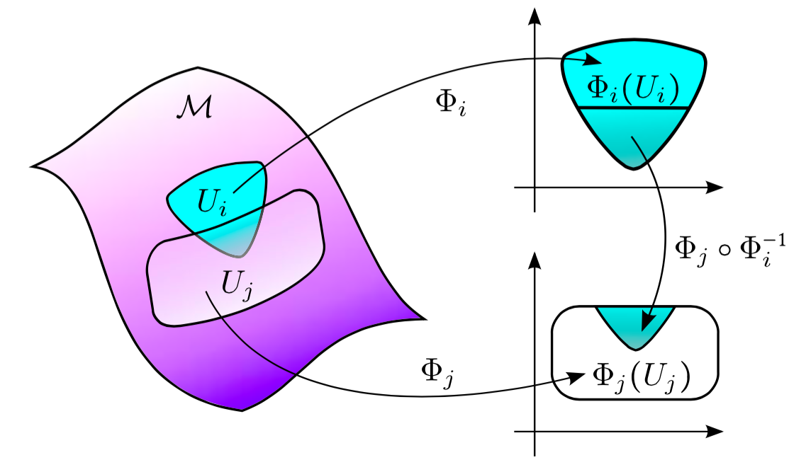
Figure 1: The transition map: the sets $\displaystyle U_{i},U_{j}\subset\mathcal{M}$ have $\displaystyle\Phi_{i}(U_{i})$ and $\displaystyle\Phi_{j}(U_{j})$ as realization into the linear space $\displaystyle\mathbb{R}^{2}$. The overlap $\displaystyle U_{i}\cap U_{j}$ should have the same realization with both $\displaystyle\Phi_{i}$ and $\displaystyle\Phi_{j}$, as it turns out in the turquoise triangle.

Finally, a natural covering of the set $\displaystyle\cal M$ is provided by a collection of compatible (each one with each other) charts. In this way all regions of $\displaystyle\cal M$ can be described by equivalent local coordinates. A collection of compatible charts covering $\displaystyle\cal M$ is called atlas. Moreover, two atlas are compatible if their union is yet an atlas of $\displaystyle\cal M$. A differentiable structure is the maximal (with respect the inclusion) atlas $\displaystyle\cal M$. Thus, a smooth manifold is the pair $\displaystyle(\mathcal{M},\mathcal{A})$ where $\displaystyle\cal A$ is a differentiable structure. Trivially, $\displaystyle\mathbb{R}^{n}$ is a smooth manifold with one chart and local coordinates given by the natural ones.

A.2 Tangent and cotangent space

Other extra structures on the manifold $\displaystyle\cal M$ are possible. The most evident example of manifold with an extra structure is the linear space $\displaystyle\mathbb{R}^{n}$: it is also a vector space. The canonical scalar product allows to introduce a metric structure on $\displaystyle\mathbb{R}^{n}$: we can measure the length of the tangent vectors, the length of the curves and the distance between two different points. Now we want introduce a metric structure also on $\displaystyle\cal M$. Doing that we obviously need a structure of vector space associated with $\displaystyle\cal M$. We know that a small region is like an open set $\displaystyle U\subset\mathbb{R}^{n}$, but as matter of fact we can not add two different points $\displaystyle p$ and $\displaystyle q$ in $\displaystyle\cal M$. The associated structure of vector space is given by the definition of the tangent space of $\displaystyle\cal M$ at a given point $\displaystyle p\in\mathcal{M}$. Thus, at any point $\displaystyle p$ we have a vector structure and so a scalar product. Then, roughly speaking, we can consider a metric structure on $\displaystyle\cal M$ as the union of all scalar product on any tangent space as $\displaystyle p$ varies on $\displaystyle\cal M$. Let us see first what is a tangent vector of $\displaystyle\cal M$ at $\displaystyle p$ and then which is the structure of the tangent space. Consider another mathematical object with one dimension, the curve, different from the line. More formally, a smooth curve is a smooth map $\displaystyle\sigma:I\rightarrow\mathbb{R}^{n}$, where $\displaystyle I\subset\mathbb{R}$ is an interval. Given $\displaystyle p\in\mathcal{M}$, we can realize a small region around $\displaystyle p$ as an open set $\displaystyle U\subset\mathbb{R}^{n}$ and perform the derivative of any differentiable function defined on it. A tangent vector of $\displaystyle\cal M$ at $\displaystyle p$ is the one $\displaystyle\sigma^{\prime}(0)$, where $\displaystyle\sigma:(-\delta,\delta)\rightarrow\mathcal{M}$ is a curve inside the small region around $\displaystyle p$ and such that $\displaystyle\sigma(0)=p$: see Fig. 2 for a major understanding of the concept. The collection of all tangent vectors of $\displaystyle\cal M$ at $\displaystyle p$ is the tangent space $\displaystyle T_{p}{\cal M}$ of $\displaystyle\cal M$ at $\displaystyle p$.

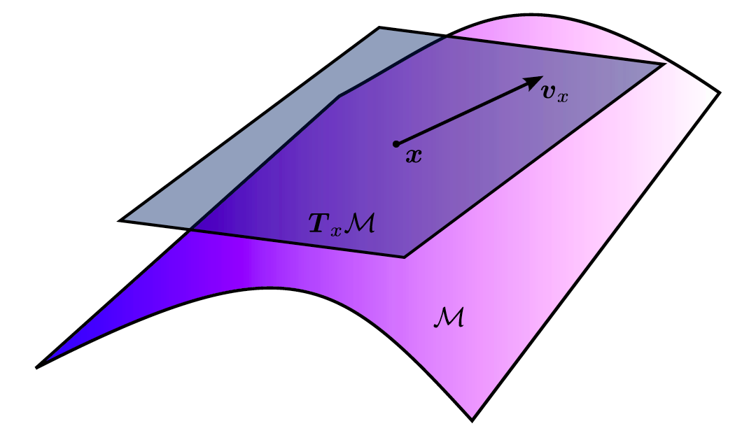
Figure 2: The tangent space of $\displaystyle\cal M$ at $\displaystyle x$: the vector $\displaystyle v_{x}$ is the tangent vector of a suitable curve $\displaystyle\sigma(t)$ living in a small region of $\displaystyle\cal M$, such that $\displaystyle\sigma(0)=x$.

In general, given an $\displaystyle n$-dimensional smooth manifold $\displaystyle\cal M$ and a point $\displaystyle p\in\mathcal{M}$, the tangent space $\displaystyle T_{p}\mathcal{M}$ of $\displaystyle\cal M$ at $\displaystyle p$ is a vector space which could be identified with the set of the partial derivatives. So, let $\displaystyle(U,\varphi)$ be the chart providing the realization of the small region around $\displaystyle p$ as an open set of $\displaystyle\mathbb{R}^{n}$, a basis of $\displaystyle T_{p}\mathcal{M}$ is given by $\displaystyle\mathcal{B}=\{\boldsymbol{\partial}_{1},\ldots,\boldsymbol{\partial}_{n}\}$, where $\displaystyle\boldsymbol{\partial}_{i}=\frac{\partial}{\partial x^{i}}$ and $\displaystyle\{x^{i}\}_{i=1}^{n}$ is the set of local coordinates.
The vector space structure $\displaystyle T_{p}\mathcal{M}$ naturally allows to define a dual vector space, the so called cotangent space $\displaystyle T_{p}^{*}\mathcal{M}$, such that every; namely if $\displaystyle\theta\in T_{p}^{*}\mathcal{M}$ and $\displaystyle\boldsymbol{X}\in T_{p}\mathcal{M}$ then $\displaystyle\theta_{p}(\boldsymbol{X})\in\mathbb{R}$. In particular, if $\displaystyle\mathcal{B}^{*}=\{dx_{p}^{1},\ldots,dx_{p}^{n}\}$ is a basis of $\displaystyle T_{p}^{*}\mathcal{M}$ then $\displaystyle dx_{p}^{i}(\partial_{j})=\delta_{ij}$
This two vector space allow to construct a tensor space of rank $\displaystyle(r,s)$, a multilinear map of the form

$$\mathcal{T}^{(r)}_{(s),p}=\otimes_{r}T_{p}\mathcal{M}\otimes_{s}T^{*}_{p}\mathcal{M}$$ (105)

an element $\displaystyle t\in\mathcal{T}^{(r)}_{(s),p}$ that in local components read

$$t=t^{i_{1}\dots i_{r}}_{j_{1}\ldots j_{s}}\boldsymbol{\partial}_{i_{1}}\otimes\boldsymbol{\partial}_{i_{r}}\otimes\mathrm{d}x_{p}^{j_{1}}\otimes\mathrm{d}x_{p}^{j_{s}}\,.$$ (106)

Fundamental operation on the tensor and their multilinear algebra are

• the linear combination of two tensor that in coordinates reads $\displaystyle\left(\alpha x+\beta y\right)^{i_{1}\ldots i_{r}}_{j_{1}\ldots j_{s}}=\alpha x^{i_{1}\ldots i_{r}}_{j_{1}\ldots j_{s}}+\beta y^{i_{1}\ldots i_{r}}_{j_{1}\ldots j_{s}}$ where $\displaystyle\alpha,\beta\in\mathbb{R}$;

• let $\displaystyle 1\leq\lambda\leq r$ and $\displaystyle 1\leq\mu\leq s$ and $\displaystyle x\in\mathcal{T}^{(r)}_{(s),p}$ then its tensor contraction $\displaystyle C_{\lambda\mu}(x)\in\mathcal{T}^{(r-1)}_{(s-1),p}$ reads in coordinate $\displaystyle(C_{\lambda\mu}(x))^{i_{1}\ldots i_{r}}_{j_{1}\ldots j_{s}}=x^{i_{1}\ldots i_{\lambda-1}ki_{\lambda+1}\ldots i_{r}}_{j_{1}\ldots j_{\mu-1}kj_{\mu+1}\ldots j_{s}}$

• the tensor product of two tensor $\displaystyle x\in x\in\mathcal{T}^{(r_{1})}_{(s_{1}),p}$ and $\displaystyle x\in\mathcal{T}^{(r_{2})}_{(s_{2}),p}$ whose action in coordinates reads

  $$\left(x\otimes y\right)^{i_{1}\ldots i_{r_{1}+r_{2}}}_{j_{1}\ldots j_{s_{1}+s_{2}}}=^{i_{1}\ldots i_{r_{1}}}_{j_{1}\ldots j_{s_{1}}}\cdot y^{i_{r_{1}+1}\ldots i_{r_{1}+r_{2}}}_{j_{s_{1}+1}\ldots j_{s_{1}+s_{2}}}$$ (107)

  this operation satisfies associative and distributive laws;

• the index permutation $\displaystyle\sigma$ that can be applied to tensors of rank $\displaystyle(r,0)$ (multivector) or $\displaystyle(0,s)$ (multiform); for instance, in the latest case we have that $\displaystyle\left(\sigma(x)\right)_{j_{1}\ldots j_{s}}=x_{j_{\sigma{1}}\ldots j_{\sigma{s}}}$. If we define the sign of a permutation as

  $$\mathrm{sgn}\sigma=\begin{cases}+1\qquad\text{even permutations}\\ -1\qquad\text{odd permutations}\\ \end{cases}$$ (108)

  we can introduce the symmetrazing map $\displaystyle S_{s}$ and the alternating map $\displaystyle A_{s}$ of a multiform $\displaystyle x\in\mathcal{T}^{(0)}_{(s),p}$

  $$\displaystyle A_{s}(x)=\dfrac{1}{s!}\sum_{\sigma\in\mathcal{S}(s)}\,\,\mathrm{sgn}\sigma\cdot\sigma{x}S_{s}(x)=\dfrac{1}{s!}\sum_{\sigma\in\mathcal{S}(s)}\,\,\sigma{x}\,\,.$$ (109)

The alternating map allows to define an exterior (wedge) product of an $\displaystyle s$-form $\displaystyle\eta$ and an $\displaystyle k$-form $\displaystyle\rho$ as

$$\eta\wedge\rho=A_{s+k}(\eta\otimes\rho)$$ (110)

with associative law, distributive law respect to sum and anticommutative law, i.e. $\displaystyle\rho\wedge\theta=(-1)^{ks}\theta\wedge\rho$. The local space of $\displaystyle k$-forms will be indicated in what follows with $\displaystyle\Lambda^{k}_{p}$.

Appendix B Tensor fields, derivations, connections and curvatures

The vector (or tensor) space introduced in the previous section are defined point-wise; the next step to enrich the structure of a differential manifolds consists in extend such structures to the whole manifold. A very simple way to realise this consists in taking the disjoint union $\displaystyle T\mathcal{M}$ of all $\displaystyle T_{p}\mathcal{M}$ with respect $\displaystyle p\in\mathcal{M}$ : this is called the tangent bundle. Analogously the disjoint union $\displaystyle T^{*}\mathcal{M}$ of all $\displaystyle T_{p}^{*}\mathcal{M}$ with respect $\displaystyle p\in\mathcal{M}$ is called the cotangent bundle. Thus, a tangent (co-tangent) bundle is a vectorial over structure upon the manifold; more in general the disjoint union of the tensor in each point $\displaystyle p\in\mathcal{M}$ of a riemanian manifold constitute the so called tensor bundle. In Fig. 3 the columns represent the vector spaces built upon the flat manifold $\displaystyle\mathbb{R}^{2}$: each column correspond to one tangent space, called fiber of the tangent bundle while the flat manifold is the base of the bundle

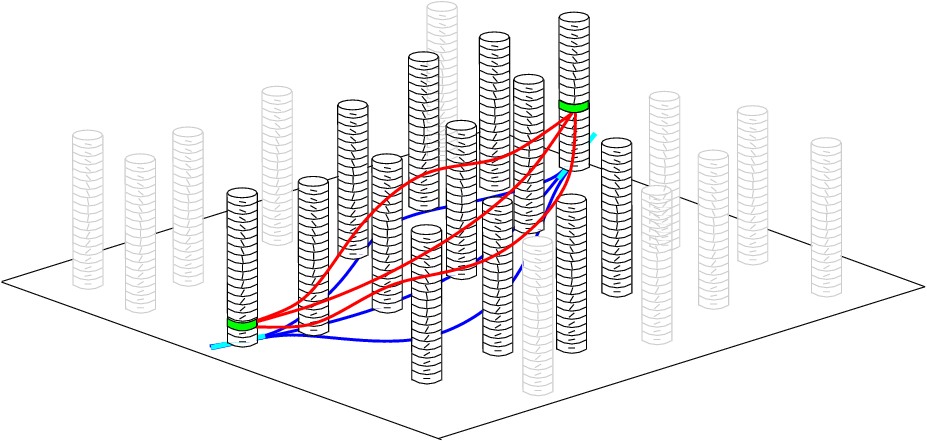
Figure 3: The tangent bundle: the columns represent the tangent spaces, called, in general, fibers of bundle. The blue lines are curves on the manifold, while the red lines are indicated as the sections of the tangent bundle upon the blue curve.

More in general the fiber can be constituted by an arbitrary vector space $\displaystyle V$ (as a space of tangent vector, covector, tensor spaces obtained as tensor product of them) and the vector bundle associated has the local structure of the Cartesian product of the manifold and the vector space: when this properties holds also globally the bundle is trivial. An application with associate at each point $\displaystyle p$ of the base $\displaystyle\mathcal{M}$ a vector in the corresponding fiber $\displaystyle V_{p}\mathcal{M}$ is a section of the fiber bundle. A vector field over a manifold $\displaystyle\mathcal{M}$ can be regarded as a section in some vector bundle $\displaystyle V\mathcal{M}$, as for instance the tangent bundle $\displaystyle T\mathcal{M}$.
In this case a vector field $\displaystyle\mathbf{X}\in\mathcal{T}_{f}\mathcal{M}$ that takes the value $\displaystyle\mathbf{X}(p)=X^{i}(p)\boldsymbol{\partial}_{i}$ in $\displaystyle p\in\mathcal{M}$ can be locally regarded as the tangent vector field of a curve $\displaystyle\gamma(t)\in\mathcal{M}$ with $\displaystyle\gamma(0)=p$ and $\displaystyle\dot{\gamma}(0)=\mathbf{X}(p)$.
The tangent bundle structure allows to introduce the operation of tensor derivation $\displaystyle\mathcal{D}\mathcal{T}^{(r)}_{{s}}\rightarrow\mathcal{T}^{(r)}_{{s}}$ that in general have to satisfy the the following properties:

• Commutes with contractions, i.e. if $\displaystyle A\in\mathcal{T}^{(r)}_{{s}}$, $\displaystyle\{V_{j}\}_{j=1,\ldots,s}\in T\mathcal{}$ and $\displaystyle\{\alpha_{i}\}_{i=1,\ldots,s}$

  $$\begin{split}&\mathcal{D}A(\theta_{1},\ldots,\theta_{i},\ldots,\theta_{r},V_{1},\ldots,V_{j},\ldots,V_{s})=(\mathcal{D}A)(\theta_{1},\ldots,\theta_{i},\ldots,\theta_{r},V_{1},\ldots,V_{j},\ldots,V_{s})+\\ &+\sum_{i=0}^{r}A(\theta_{1},\ldots,\mathcal{D}\theta_{i},\ldots,\theta_{r},V_{1},\ldots,V_{j},\ldots,V_{s})+\\ &+\sum_{j=1}^{s}A(\theta_{1},\ldots,\theta_{i},\ldots,\theta_{r},V_{1},\ldots,\mathcal{D}V_{j},\ldots,V_{s})\end{split}$$ (111)

• satisfy a Leibniz law with respect to tensor product, i.e. $\displaystyle\mathcal{D}(A\otimes B)=\mathcal{D}A\otimes B+A\otimes\mathcal{D}B$.

From this two properties is follows that the action of a derivation is specified by its action over function and vector field. The Lie derivative $\displaystyle\mathcal{L}_{\boldsymbol{X}}$ with respect to a vector field $\displaystyle\mathbf{X}$ generalize the concept of derivation along a curve: it measure the local rate of change of a tensor field along a curve whose tangent vector is $\displaystyle\mathbf{X}$. Its action over functions $\displaystyle f$ and vector fields $\displaystyle Y\in T\mathcal{M}$ is given by:

$$\mathcal{L}_{\mathbf{X}}f:=\mathbf{X}(f)=X^{i}\partial_{i}f\qquad\mathcal{L}_{\mathbf{X}}\mathbf{Y}=[\mathbf{X},\mathbf{Y}]=\left(X^{j}\partial_{j}Y^{i}-Y^{j}\partial_{j}X^{i}\right)\boldsymbol{\partial}_{i}$$ (112)

and consequently its action on one form is given by $\displaystyle\mathcal{L}_{\mathbf{X}}(\theta)=\left(\mathcal{L}_{\mathbf{X}}\theta\right)_{i}\mathrm{d}x^{i}=X^{i}\partial_{i}\theta_{j}+\theta_{j}\partial_{i}X^{i}$.
We notice that to calculate the values of the derivative of a tensor with respect to a vector field $\displaystyle\mathbf{X}$ in a point $\displaystyle p$ it is not sufficient to know its point-wise value but it is required its local value for the presence of its derivatives. Moreover this derivation cannot be applied to a general vector bundle constructed over $\displaystyle\mathcal{M}$. For this latest case is required to introduce the concept of connection over a vector bundle. Let be $\displaystyle\Gamma(E)$ the set of all sections over a $\displaystyle q$-dimensional vector bundle $\displaystyle E$ with base $\displaystyle\mathcal{M}$ and fibre $\displaystyle V$ ; then a connection $\displaystyle\nabla$ over this vector bundle is a map $\displaystyle\nabla:\Gamma(E)\rightarrow\Gamma(T*\mathcal{M}\otimes E)$ such that

• the connection of a sum of sections is the sum of the connections of each section, i.e. $\displaystyle s_{1},s_{2}\in\Gamma(E)$ it follows that $\displaystyle\nabla(s_{1}+s_{2})=\nabla s_{1}+\nabla s_{2}$;

• if $\displaystyle f$ is a function over $\displaystyle\mathcal{M}$ and $\displaystyle s\in\Gamma(E)$ then $\displaystyle\nabla(fs)=\mathrm{d}f\otimes s+f\nabla s$ where $\displaystyle\mathrm{d}f=\partial_{i}f\mathrm{d}x^{i}$ is the differential of the function.

When the connection $\displaystyle\nabla s$ is contracted with a vector field $\displaystyle\mathbf{X}\in T\mathcal{M}$ is called covariant derivative of $\displaystyle s$ with respect to $\displaystyle\mathbf{X}$ and it is indicated with $\displaystyle\nabla_{\mathbf{X}}s$. The action of the connection is characterized by matrix valued $\displaystyle 1$-form, called connection form $\displaystyle\theta$: if $\displaystyle\mathbf{s}=s^{\alpha}\mathbf{e}_{\alpha}$ is a section in vector bundle $\displaystyle V$ whose local basis is $\displaystyle\{\mathbf{e}_{\alpha}\}_{\alpha=1,...,q}$

$$\nabla s=\mathrm{d}s^{\alpha}\otimes\mathbf{e}_{\alpha}+s^{\beta}\theta_{\beta}^{\alpha}\mathbf{e}_{\alpha}=\left(\partial_{i}s^{\alpha}+s^{\beta}\theta_{\beta;i}^{\alpha}\right)\mathrm{d}x^{i}\otimes\mathbf{e}_{\alpha}\,.$$ (113)

Covariant derivative with respect to $\displaystyle\mathbf{X}=X^{i}\boldsymbol{\partial}_{i}$ on a tensor bundle $\displaystyle\mathcal{T}^{(r)}_{(s)}\mathcal{M}$ acts like a derivation; it follows that also in this case it is uniquely defined by its action on function and vectors

$$\nabla_{\mathbf{X}}f=X^{i}\partial_{i}f\qquad\nabla_{\boldsymbol{X}}\mathbf{Y}=X^{j}\left(\partial_{j}Y^{i}+Y^{k}\theta^{i}_{k;j}\right)\boldsymbol{\partial}_{i}$$ (114)

and consequently, in the case of the covariant derivative with respect to $\displaystyle\mathbf{X}$ of a general tensor $\displaystyle t=t^{i_{1}\ldots i_{s}}_{j_{1}\ldots j_{r}}\boldsymbol{\partial}_{i_{1}}\otimes\ldots\boldsymbol{\partial}_{i_{s}}\otimes\mathrm{d}x^{j_{1}}\otimes\ldots\mathrm{d}x^{j_{r}}$ it is given by

$$(\nabla_{\mathbf{X}}t)^{i_{1}\ldots i_{s}}_{j_{1}\ldots j_{r}}=X^{k}\left(\partial_{k}t^{i_{1}\ldots i_{s}}_{j_{1}\ldots j_{r}}+\sum_{l=1}^{r}\theta^{i_{l}}_{i_{m};k}t^{i_{1}\ldots i_{m}\ldots i_{s}}_{j_{1}\ldots j_{r}}-\sum_{l=1}^{s}\theta^{j_{m}}_{j_{l};k}t^{i_{1}\ldots i_{m}\ldots i_{s}}_{j_{1}\ldots j_{r}}\right)$$ (115)

For connections on the tangent bundle, the torsion $\displaystyle(2,1)$-rank tensor is defined as

$$\mathrm{Tor}(\mathbf{X},\mathbf{Y})=\nabla_{\mathbf{X}}\mathbf{Y}-\nabla_{\mathbf{Y}}\mathbf{X}-[\mathbf{X},\mathbf{Y}]$$ (116)

and in components reads

$$\mathrm{Tor}_{ij}^{k}=\theta_{i;j}^{k}-\theta_{j;i}^{k}-\left([\boldsymbol{\partial}_{i},\boldsymbol{\partial}_{j}]\right)^{k}\,.$$ (117)

In general $\displaystyle\nabla_{\mathbf{X}}\nabla_{\mathbf{Y}}\neq\nabla_{\mathbf{Y}}\nabla_{\mathbf{X}}$ a measure of the difference between these derivatives is the curvature $\displaystyle R$ of the connection, i.e.

$$R(\mathbf{X},\mathbf{Y})=\nabla_{\mathbf{X}}\nabla_{\mathbf{Y}}-\nabla_{\mathbf{Y}}\nabla_{\mathbf{X}}-\nabla_{[\mathbf{X},\mathbf{Y}]}$$ (118)

Appendix C Differential forms, exterior differentiations, integration of forms

Let us indicate with $\displaystyle A^{k}(\mathcal{M})$ the tensor bundle constructed over the manifold $\displaystyle\mathcal{M}$ as a disjoint union of the $\displaystyle k$-form spaces $\displaystyle\Lambda^{k}_{p}$. For the $\displaystyle n$-dimensional manifold $\displaystyle\mathcal{M}$ the space $\displaystyle A(\mathcal{M})=\sum_{k=0}^{n}A^{k}(\mathcal{M})$ is a graded algebra as with respect to the operation of sum $\displaystyle+$ and wedge product $\displaystyle\wedge$ of differential forms, meaning that $\displaystyle A(\mathcal{M})$ is a direct sum of a sequence of a vector spaces, and the product $\displaystyle\wedge$ defines a map $\displaystyle\wedge:A^{r}(\mathcal{M})+A^{s}(\mathcal{M})\rightarrow A^{r+s}(\mathcal{M})$ where $\displaystyle A^{r+s}(\mathcal{M})$ is zero when $\displaystyle r+s>n$. The exterior derivative $\displaystyle\mathrm{d}$ is a derivation introduced on $\displaystyle A(\mathcal{M})$ such that $\displaystyle\mathrm{d}(A^{k}(\mathcal{M}))\subset A^{k+1}(\mathcal{M})$ such that for any $\displaystyle\alpha,\beta\in A(\mathcal{M})$:

• $\displaystyle\mathrm{d}(\alpha+\beta)=\mathrm{d}\alpha+\mathrm{d}\beta$;

• if $\displaystyle\alpha\in A^{r}(\mathcal{M})$ then $\displaystyle\mathrm{d}(\alpha\wedge\beta)=\mathrm{d}\alpha\wedge\beta+(-1)^{r}\alpha\wedge\mathrm{d}\beta$;

• if $\displaystyle f$ is a smooth function $\displaystyle\mathcal{M}$ (i.e. $\displaystyle f\in A^{0}(\mathcal{M})$), where $\displaystyle\mathrm{d}f=\partial_{i}f\mathrm{d}x^{i}$

• if $\displaystyle f$ is a smooth function $\displaystyle\mathcal{M}$ then $\displaystyle\mathrm{d}(\mathrm{d}f)=0$.

The exterior differentiation of a differential $\displaystyle k$-form $\displaystyle\alpha\in A^{k}(\mathcal{M})$ is given by

$$\begin{split}&\left(\mathrm{d}\alpha\right)\left(\mathbf{X}_{1},\ldots,\mathbf{X}_{k+1}\right)=\sum_{i=1}^{k+1}(-1)^{i+1}\mathbf{X}_{i}\left(\alpha(\mathbf{X}_{1},\ldots,\mathbf{X}_{i-1},\mathbf{X}_{i+1},\ldots\mathbf{X}_{k+1})\right)+\\ &+\sum_{1\leq i<j\leq k+1}(-1)^{i+j}\alpha([\mathbf{X}_{i},\mathbf{X}_{j}],\mathbf{X}_{1},\ldots\mathbf{X}_{i-1}\mathbf{X}_{i+1}\ldots\mathbf{X}_{j-1}\mathbf{X}_{j+1}\ldots\mathbf{X}_{k+1})\end{split}$$ (119)

The Poincare’s Lemma states that $\displaystyle\mathrm{d}^{2}\alpha=0$ for all $\displaystyle\alpha\in A(\mathcal{M})$. The space $\displaystyle A(\mathcal{M})$ endowed with the differential $\displaystyle\mathrm{d}$ is called a complex. In any subspace $\displaystyle A^{k}(\mathcal{M})$ two subspaces can be identified:

• the space $\displaystyle Z^{k}(\mathcal{M})$ of all $\displaystyle k$-forms $\displaystyle\alpha$ that are closed, so $\displaystyle\mathrm{d}\alpha=0$, (also called cocycles)

• the space $\displaystyle B^{k}(\mathcal{M})$ of all $\displaystyle k$-forms $\displaystyle\alpha$ that are exact, so that exist $\displaystyle\beta\in C^{k-1}(\mathcal{M})$ such that $\displaystyle\mathrm{d}\beta=\alpha$, (also called coboundaries).

The cohomology space $\displaystyle H^{k}(\mathcal{M};\mathbb{R})$ is defined as

$$H^{k}(\mathcal{M};\mathbb{R})=Z^{k}(\mathcal{M})/B^{k}(\mathcal{M})$$ (120)

and an element $\displaystyle[\omega]$ in this space is the equivalence class of $\displaystyle k$-forms that differ among them for an exact form, i.e. $\displaystyle[\omega_{1}]=[\omega_{2}]$ if $\displaystyle\omega_{1}-\omega_{2}=\mathrm{d}phi$. From the definition of differential $\displaystyle k$-form it follows that $\displaystyle H^{k}(\mathcal{M},\mathbb{R})=0$ if $\displaystyle k>n$.
The De Rham cohomology space $\displaystyle H^{*}(\mathcal{M};\mathbb{R})$ is a graded space obtained as the direct sum of the $\displaystyle k$-dimensional cohomology spaces:

$$H^{*}(\mathcal{M},\mathbb{R})=\otimes_{k\geq 0}H^{k}(\mathcal{M};\mathbb{R})\,.$$ (121)

and it is a multiplication ring with the the addition $\displaystyle[\omega_{1}]+[\omega_{2}]=[\omega_{1}+\omega_{2}]$ and the multiplication $\displaystyle[\omega_{1}]\smile[\omega_{2}]=[\omega_{1}\wedge\omega_{2}]$. Moreover if $\displaystyle f:\mathcal{M}^{n}\rightarrow\mathcal{N}^{k}$ is a smooth map the pullback $\displaystyle f^{*}:A^{p}(\mathcal{N}^{k})\rightarrow A^{k}(\mathcal{M}^{n})$ is a homomorphism induced by the mapping among cohomology rings, i.e. $\displaystyle f^{*}:H^{*}(\mathcal{N}^{k};\mathbb{R})\rightarrow H^{*}(\mathcal{M}^{k};\mathbb{R})$ with $\displaystyle f^{*}[\omega]=[f^{*}\omega]$.
Two smooth mapping $\displaystyle f_{0}:\mathcal{M}^{n}\rightarrow\mathcal{N}^{k}$ and $\displaystyle f_{1}:\mathcal{M}^{n}\rightarrow\mathcal{N}^{k}$ are smoothly homotopic if there is a smooth homotopy mapping $\displaystyle F:\mathcal{M}^{n}\times[0,1]\rightarrow\mathcal{N}^{k}$ such that $\displaystyle F(x,k)=f_{k}(x)$ with $\displaystyle k=0,1$. In this case the action of the homomorphism of cohomology rings $\displaystyle f^{*}_{0}:H^{*}(\mathcal{N}^{k};\mathbb{R})\rightarrow H^{*}(\mathcal{M}^{n};\mathbb{R})$ and $\displaystyle f^{*}_{1}:H^{*}(\mathcal{N}^{k};\mathbb{R})\rightarrow H^{*}(\mathcal{M}^{n};\mathbb{R})$ coincides. Two manifolds $\displaystyle\mathcal{M}^{n}$ and $\displaystyle\mathcal{N}^{n}$ are said to be homotopically equivalent if there exists two mappings $\displaystyle f:\mathcal{M}^{n}\rightarrow\mathcal{N}^{k}$ and $\displaystyle g:\mathcal{N}^{k}\rightarrow\mathcal{M}^{n}$ such that $\displaystyle fg$ and $\displaystyle gf$ are homotopic to the identity. It can be proved that two homotopically equivalent manifolds have isomorphic cohomology groups.
The integration of exterior derivatives allows to connect local and global properties of a manifold. The first step consists in defining an orientable manifold as $\displaystyle n$-dimensional manifold $\displaystyle\mathcal{M}$ where there exists a continuous and nonvanishing exterior differential $\displaystyle n$-form; two differential $\displaystyle n$-forms which differ everywhere by a function factor which is always positive define an orientation. Let us suppose that $\displaystyle\mathcal{M}$ is a manifold oriented by a differential $\displaystyle n$-form $\displaystyle\omega$, then a chart $\displaystyle(U,x)$ is compatible if $\displaystyle\omega$ and $\displaystyle\mathrm{d}x^{1}\wedge\ldots\wedge\mathrm{d}x^{n}$ define the same orientation.
The main results that allows to define the integration over a manifold is the Partition of Unity Theorem: suppose $\displaystyle\Sigma$ is an open covering of a smooth manifold $\displaystyle\mathcal{M}$. Then there exists a family of smooth functions $\displaystyle\{g_{\alpha}\}$ on $\displaystyle\mathcal{M}$ satisfying the following conditions:

• $\displaystyle 0\leq g_{\alpha}\leq 1$ and the $\displaystyle\mathrm{supp}g_{\alpha}=\{p\in\mathcal{M}|g_{\alpha}(p)\neq 0\}$ is compact for each $\displaystyle\alpha$. Moreover, there exists an open set $\displaystyle W_{i}\in\Sigma$ such that $\displaystyle g_{\alpha}\subset W_{i}$;

• For each point $\displaystyle p\in\mathcal{M}$ there is a neighbourhood $\displaystyle U$ that intersects $\displaystyle\mathrm{supp}g_{\alpha}$ for only a finite number of $\displaystyle\alpha$

• $\displaystyle\sum_{\alpha}g_{\alpha}=1$.

The integral of a differential $\displaystyle m$-form $\displaystyle\omega$ is defined as

$$\int_{\mathcal{M}}\omega=\sum_{\alpha}\int_{W_{i}}g_{alpha}\omega$$ (122)

where in a local coordinate system $\displaystyle g_{alpha}\omega=f(x^{1},\ldots,x^{n})\mathrm{d}x^{1}\wedge\ldots\wedge\mathrm{d}x^{n}$ so that $\displaystyle\int_{W_{i}}\,\,g_{alpha}\omega=\int_{W_{i}}f(x^{1},\ldots,x^{n})\mathrm{d}x^{1}\ldots\mathrm{d}x^{n}$. Let us suppose that $\displaystyle h:\mathcal{N}\rightarrow\mathcal{M}$ is the imbedding of a $\displaystyle k$-dimensional submanifold in the $\displaystyle n$-dimensional ambient manifold $\displaystyle\mathcal{M}$. Then the integral of the differential $\displaystyle k$-form $\displaystyle h^{*}\omega$ over $\displaystyle\mathcal{N}$ is defined as

$$\int_{h(\mathcal{N})}\omega=\int_{\mathcal{N}}h^{*}\omega\,\,\,.$$ (123)

A very relevant result in integration theory of differential forms is the Stokes Theorem: let $\displaystyle\omega$ be a $\displaystyle(n-1)$-form and $\displaystyle D\subseteq\mathcal{M}$ and with a smooth or piecewise smooth boundary $\displaystyle\partial D$ then

$$\int_{\partial D}\omega=\int_{D}\mathrm{d}\omega\,\,\,.$$ (124)

This formula has its importance as it allows to characterize the topology of a certain domain $\displaystyle D$ over a manifold $\displaystyle\mathcal{M}$ as it establishes a duality (Poincaré duality) among the boundary operator $\displaystyle\partial$ and the coboundary operator (i.e. the exterior differentiation) $\displaystyle\mathrm{d}$ on forms. This result can be expressed

$$\int_{\partial D}\omega=(\partial D,\omega)=(D,\mathrm{d}\omega)=\int_{D}\mathrm{d}\omega$$ (125)

which represents the link between homology, the rigorous mathematical way to classify the manifolds with respect to their "holes", and the De Rham cohomology of differential forms on manifolds.
A geometric cycle on a manifold $\displaystyle\mathcal{M}^{n}$ is a pair $\displaystyle(\mathcal{N}^{k},f)$ consisting of a smooth mapping $\displaystyle f:\mathcal{N}^{k}\rightarrow\mathcal{M}^{n}$. If there is an orientation on the manifold $\displaystyle\mathcal{N}^{k}$, then such a cycle will be said to be oriented. Any closed $\displaystyle k$-form $\displaystyle\omega$ on a manifold $\displaystyle\mathcal{M}^{n}$ specifies a function on the set of all $\displaystyle k$-dimensional cycles $\displaystyle z=(\mathcal{N}^{k},f)$ by the formula

$$\left\langle\omega,z\right\rangle=\int_{N_{k}}f^{*}\omega\,.\,.$$ (126)

It can be proved that the value of $\displaystyle\left\langle\omega,z\right\rangle$ depends only by the cohomology group $\displaystyle[\omega]$.
Let $\displaystyle A_{p}(\mathcal{M})$ the space generated by all the oriented $\displaystyle p$-cycle over the field $\displaystyle\mathbb{R}$. For each element $\displaystyle z$ of this space we can define the integral of a closed $\displaystyle p$-form $\displaystyle\omega$ over $\displaystyle z$. Namely let $\displaystyle z=\lambda_{1}z_{1}+\ldots+\lambda_{k}z_{k}$ where $\displaystyle\lambda_{i}\in\mathbb{R}$ and $\displaystyle z_{i}=(\mathcal{N}_{i}^{p},f_{i})$ are ordinary cycles. Then

$$\left\langle\omega,z\right\rangle=\sum_{i}\lambda_{i}\left\langle\omega,z_{i}\right\rangle=\sum_{i}\lambda_{i}\int_{\mathcal{N}_{i}}f_{i}^{*}\omega$$ (127)

Let $\displaystyle B_{p}(\mathcal{M})\subset A_{p}(\mathcal{M})$ be the subspace that consist of the cycles such that the integral of all closed $\displaystyle p$-forms over these cycles vanish. The quotient space

$$H_{p}(\mathcal{M}^{p};\mathbb{R})=A_{p}(\mathcal{M}^{n})/B_{p}(\mathcal{M}^{n})$$ (128)

is called the real $\displaystyle p$-dimensional homology group of the manifold $\displaystyle\mathcal{M}^{n}$. The homology space is dual to the cohomology group $\displaystyle H^{p}(\mathcal{M}^{p};\mathbb{R})$ and for any nonzero element $\displaystyle[\omega]\in H^{p}(\mathcal{M}^{p};\mathbb{R})$ the linear functional

$$\left\langle[\omega],[z]\right\rangle=\left\langle\omega,z\right\rangle\qquad z\in H_{p}(\mathcal{M}^{p};\mathbb{R})\,.$$ (129)

For compact manifolds all the cohomology groups are finite-dimensional and their dimensions are called Betti numbers $\displaystyle b_{p}(\mathcal{M})=\mathrm{dim}H_{p}(\mathcal{M}^{p};\mathbb{R})=\mathrm{dim}H^{p}(\mathcal{M}^{p};\mathbb{R})$ and are topological invariants. The alternating sum of the Betti numbers is the Euler characteristics $\displaystyle\chi(\mathcal{M})=\sum_{i=0}^{n}(-1)^{i}\,b_{i}(\mathcal{M})$; as for a compact $\displaystyle n$-dimensional connected manifold without boundaries the Poincare duality implies $\displaystyle H^{n-k}(\mathcal{M}^{p};\mathbb{R})=H^{k}(\mathcal{M}^{p};\mathbb{R})$ it follows that for odd-dimensional manifolds the Euler characteristic vanishes $\displaystyle\chi(\mathcal{M}^{2n+1})=0$.

Appendix D Riemannian structure

Thanks to the vector structure, a scalar product, can be defined on $\displaystyle T_{p}\mathcal{M}$ as $\displaystyle g_{p}:T_{p}\mathcal{M}\times T_{p}\mathcal{M}\rightarrow\mathbb{R}$. This is a way to associate a real number to any pair $\displaystyle(\mathbf{X}_{p},\mathbf{Y}_{p})$ of tangent vectors. This product inherits all the features of the canonical scalar product on the linear space $\displaystyle\mathbb{R}^{n}$; in particular $\displaystyle\|\mathbf{X}_{p}\|_{g_{p}}^{2}=g_{p}(\mathbf{X}_{p},\mathbf{X}_{p})>0$ for all tangent vector $\displaystyle\mathbf{X}_{p}$ and $\displaystyle g_{p}(\mathbf{X}_{p},\mathbf{Y}_{p})=0$, if and only if one of the tangent vectors $\displaystyle X_{p}$ or $\displaystyle Y_{p}$ is null.
The Riemannian structure allows to define the gradient $\displaystyle\mathbf{grad}_{g}f$ of a function $\displaystyle f$ on $\displaystyle\mathcal{M}$ as the vector field with the property

$$g(\mathbf{grad}_{g}f,\mathbf{Y})=\mathbf{Y}(f)=Y^{i}\partial_{i}f\,.$$ (130)

and the divergence of a vector field $\displaystyle\mathbf{X}$ as

$$\left(\mathrm{div}_{g}\mathbf{X}\right)=\sum_{j=1}^{N}\,\,\mathrm{d}x^{j}\left(\nabla_{\boldsymbol{\partial}_{j}}\mathbf{X}\right)\,\,.$$ (131)

If this properties holds for every point $\displaystyle p\in\mathcal{M}$ for the tensor field $\displaystyle(0,2)$-rank $\displaystyle g=g_{ij}\mathrm{d}x^{i}\otimes\mathrm{d}x^{j}$ such a tensor is a metric tensor field that defines a Riemannian structure over the manifold $\displaystyle\mathcal{M}$.
The definition of a metric tensor allows to define the length of a curve $\displaystyle c(t):[a,b]\rightarrow\mathbb{R}$ as

$$L(c)=\int_{a}^{b}\|\dot{\mathbf{c}}(t)\|^{2}\mathrm{d}t\,.$$ (132)

and the volume form $\displaystyle\mathrm{d}\mathrm{Vol}_{g}$

$$\mathrm{d}\mathrm{Vol}_{g}=|\mathrm{det}g_{ij}|^{1/2}\mathrm{d}x^{1}\wedge\ldots\wedge\mathrm{d}x^{N}\,.$$ (133)

The inverse of $\displaystyle g_{ij}$ is given by the $\displaystyle g^{kl}$ matrix with $\displaystyle g_{ij}g^{jk}=\delta_{i}^{k}$; this two matrices allows to define the raising and lowering of indices of a tensor, i.e.

$$g_{ki_{l}}t_{\quad\quad\quad j_{1}\ldots j_{r}}^{i_{1}\ldots i_{l}\ldots i_{r}}=t_{\quad\quad\quad k\quad\quad\quad j_{1}\ldots j_{r}}^{i_{1}\ldots i_{l-1}\quad i_{l+1}\ldots i_{r}}\qquad\qquad g^{kj_{l}}t_{\quad\quad j_{1}\ldots j_{l}\ldots j_{r}}^{i_{1}\ldots i_{r}}=t_{\quad\quad j_{1}\ldots j_{l-1}\quad j_{l+1}\ldots j_{r}}^{i_{1}\ldots i_{r}\quad\quad\quad k}$$ (134)

This allows to define the metric-dependent trace of a $\displaystyle(0,2)$-rank tensor $\displaystyle A=A_{ij}\mathrm{d}x^{i}\otimes\mathrm{d}x^{j}$ as:

$$\mathrm{Tr}^{g}\left(A\right)=g^{ij}A_{ij}=A^{i}_{\quad i}\,.$$ (135)

The Riemannian structure puts some constraints on the definition of a connection on the tangent and tensor bundles over a given manifold; in particular, a Levi-Civita connection is compatible with the metric, that means

$$\left(\nabla_{\mathbf{X}}g\right)_{ij}=X^{k}\partial_{k}g_{ij}-\theta^{l}_{i;k}g_{lj}-\theta^{l}_{j;k}g_{il}$$ (136)

and torsion free, i.e. $\displaystyle\mathrm{Tor}=0$. In this case the components of the matrix-valued connection form are expressed by the Christoffel symbol $\displaystyle\Gamma^{k}_{ij}=\theta^{k}_{j;i}$. It can be proved that the for a given metric $\displaystyle g$ over $\displaystyle\mathcal{M}$ a unique Levi-Civita is defined.
The Christoffel symbol can be expressed as a function of derivatives of the components of the metric tensor

$$\Gamma^{i}_{jk}=\dfrac{1}{2}g^{il}\left(\partial_{j}g_{lk}+\partial_{k}g_{jk}-\partial_{l}g_{jk}\right)\,.$$ (137)

The curvature tensor for a Levi-Civita connection specified by the symbols $\displaystyle\Gamma^{i}_{jk}$ is the Riemann curvature tensor that in components reads:

$$R^{i}_{jkl}=\partial_{l}\Gamma^{i}_{jk}-\partial_{j}\Gamma^{i}_{kl}+\Gamma^{m}_{jk}\Gamma^{i}_{ml}-\Gamma^{m}_{jl}\Gamma^{i}_{mk}$$ (138)

and whose completely covariant version is the tensor $\displaystyle R_{ijkl}=g_{mi}R^{i}_{jkl}$ with basic symmetries:

$$R_{ijkl}=-R_{jikl}=-R_{ijlk}=R_{klij}\,.$$ (139)

In order to give a geometrical interpretation of Riemann curvature, let us introduce the concept geodesic curve as the shortest smooth curve that connects two points on a Riemannian manifold; a variational formulation of this condition for a geodesic $\displaystyle\gamma=(x^{1}(t)\ldots x^{N}(t)))$ is given by:

$$\Delta_{\dot{\boldsymbol{\gamma}}}\dot{\boldsymbol{\gamma}}=0\quad\Rightarrow\quad\ddot{x}^{i}+\Gamma^{i}_{kj}\ddot{x}^{j}\ddot{x}^{k}\,.$$ (140)

Now let us consider a smooth one parameter family of geodesic $\displaystyle\gamma_{\tau}$ with $\displaystyle\gamma_{0}(t)=\gamma(t)$ than the Jacobi vector field $\displaystyle\mathbf{J}$ along the geodesic $\displaystyle\gamma(t)$ is defined as

$$\mathbf{J}=\partial\gamma_{\tau}(t)\Bigr{|}_{\tau=0}$$ (141)

The Riemann curvature tensor gives a measure of the local geodesic spread. The evolution of the Jacobi field along a given geodesic is described by the Jacobi-Levi-Civita equation. Let us suppose that along the geodesic it is consider a orthonormal frame $\displaystyle\{\mathbf{e}_{i}\}_{i=1,...,N}$ in $\displaystyle T_{\gamma(t)}\mathcal{M}$, parallel transported all along $\displaystyle\Delta\mathbf{e}_{i}=0$ and with $\displaystyle\mathbf{e}_{1}=\dot{\boldsymbol{\gamma}}/\|\dot{\boldsymbol{\gamma}}\|_{g}$ than if the jacobi vector field is expressed $\displaystyle\boldsymbol{J}=y^{i}\mathbf{e}_{i}$ the Jacobi Levi Civita for the geodesic spread reads

$$\ddot{y}^{k}+\|\dot{\boldsymbol{\gamma}}\|^{2}_{g}\mathrm{R}^{k}_{1j1}y^{j}=0\,.$$ (142)

The contraction $\displaystyle C_{1,2}(R)$ of the Riemann curvature tensor is the Ricci curvature tensor

$$\mathrm{Ric}_{ij}=R^{k}_{ikj}=\partial_{l}\Gamma^{l}_{ji}-\partial_{j}\Gamma^{l}_{li}+\Gamma^{l}_{lk}\Gamma^{k}_{ji}-\Gamma^{l}_{jk}\Gamma^{k}_{il}\,.$$ (143)

For a given metric $\displaystyle g$ the Ricci curvature gives a local measure of the difference between the volume form with respect to an euclidean metric $\displaystyle g_{\mathbb{E}}$, i.e. if in a certain point $\displaystyle g_{ij}=\delta_{ij}+o\left(\|\mathbf{X}\|_{g}^{2}\right)$ with $\displaystyle\mathbf{X}=X^{i}\boldsymbol{\partial}_{i}$

$$\mathrm{d}\mathrm{Vol}_{g}=\mathrm{d}\mathrm{Vol}_{g_{\mathbb{E}}}\left(1-\dfrac{1}{6}\mathrm{Ric}_{jk}X^{k}X^{j}+o\left(\|\mathbf{X}\|_{g}^{3}\right)\right)$$ (144)

so in the directions $\displaystyle\mathbf{X}$ such that $\displaystyle\mathrm{Ric}(\boldsymbol{X},\boldsymbol{X})$ is positive the volume is contracted with respect to the Euclidean volume.
The metric-dependent trace of the Ricci curvature tensor is the Scalar curvature $\displaystyle\mathcal{R}=\mathrm{Tr}^{g}\mathrm{Ric}=g^{ij}\mathrm{Ric}_{ij}$.

Appendix E Riemmanian geometry of codimension one submanifolds (regular level sets)

Let $\displaystyle(\mathcal{M},\bar{g})$ be a $\displaystyle N$-dimensional Riemannian manifold whose Levi-Civita commection is $\displaystyle\overline{\nabla}$. A regular Submanifold of dimension $\displaystyle K$ is a subset $\displaystyle\Sigma$ such that for every point $\displaystyle p\in\Sigma$ such that for a certain chart $\displaystyle(U,x)$ over $\displaystyle\mathcal{M}$ it holds $\displaystyle x\left(U\cap Sigma\right)=x(U)\cup{\mathbb{R}^{K}\times\{c\}}$ for some $\displaystyle c\in\mathbb{R}^{N-K}$, that means that exists a chart over $\displaystyle\mathcal{M}$ such that for its restriction over $\displaystyle\Sigma$ there are $\displaystyle N-K$ fixed components. In particular, the set defined as a locus that in a chart $\displaystyle(U,x)$ reads $\displaystyle\Sigma=\left\{p\in\mathcal{M}|f_{A}(x^{1}(p),...,x_{N}(p))\right\}=0\qquad\text{for}\,\,A=1,...,L$ it is a $\displaystyle K$-dimensional level sets (with $\displaystyle K\leq L$) if the rank of the Jacobian $\displaystyle\partial_{i}f_{A}$ is $\displaystyle K$.
The equipotential level sets discussed in the first part of this manuscript are an example of regular submanifold without boundaries in absence of critical point of potential energy. Moreover in this specific case, we have a local regular foliation $\displaystyle\mathcal{F}$ of the configuration space, namely when the ambient manifolds can be regarded as the disjoint union of connected regular submanifolds $\displaystyle\Sigma_{\mathbf{a}\in\mathbb{R}^{N-K}}$ called leaves of dimension $\displaystyle K$ (and co-dimension $\displaystyle N-K$) such that in a neighbourhood of any point of the ambient space exists a chart $\displaystyle(U,x)$ such where the coordinate can be expressed in the form $\displaystyle(a^{1},...,a^{N-K},x^{1},...,x^{K})$. In what follows we consider level sets of one single function so that $\displaystyle K=N-1$.
As we supposed that the ambient space has a Riemannian structure, each leaf inherits a metric structure, the so called First Fundamental Form $\displaystyle\mathrm{I}:T_{p}\Sigma\times T_{p}\Sigma\rightarrow\mathbb{R}$ defined over a regular submanifold of co-dimension one

$$\mathrm{I}_{\Sigma}(\mathbf{X},\mathbf{Y}):\equiv\bar{g}(\mathbf{X},\mathbf{Y})\qquad\mathbf{X},\mathbf{Y}\in T_{p}\Sigma$$ (145)

and it coincides with the restriction of metric tensor $\displaystyle\bar{g}$ on the immersed co-dimension one submanifold $\displaystyle\Sigma$. This allows to define a Levi-Civita connection $\displaystyle\nabla$ over the regular submanifold. In order to introduce a more suitable notation for a fixed $\displaystyle\Sigma$, we will use in what follows $\displaystyle g=\mathrm{I}$.
Moreover, for a co-dimension one regular submanifold $\displaystyle\Sigma$ in a ambient space $\displaystyle\mathcal{M}$ it is possible to define a normal vector field as the vector field $\displaystyle\boldsymbol{\nu}\neq\mathbf{0}$ such that $\displaystyle\bar{g}(\boldsymbol{\nu},\mathbf{X})=0$ for every $\displaystyle\mathbf{X}\in T_{p}\Sigma$.
The rate of (covariant) variation of the normal vector field in a direction tangent to the submanifolds defines is intuitively related with the concept of curvature for a immersed submanifold. This is can be formalized as follows. First of all let us consider the Weingarten operator or Shape Operator $\displaystyle W_{\boldsymbol{\nu}_{p}}:T_{p}\Sigma\rightarrow T_{p}\Sigma$:

$$W_{\boldsymbol{\nu}_{p}}(X):\equiv\overline{\nabla}_{\mathbf{X}}\boldsymbol{\nu}\bigr{|}_{p}\qquad\mathbf{X}\in T_{p}\Sigma\,\,\,\,\,.$$ (146)

This operator can be regarded as $\displaystyle(1,1)$-rank tensor field over he submanifold tangent space; the induced metric structure over the submanifold allows to construct a $\displaystyle(0,2)$-rank tensor field over this submanifold called Second Fundamental Form $\displaystyle\mathrm{II}_{\Sigma}:T_{p}\Sigma\times T_{p}\Sigma\rightarrow\mathbb{R}$

$$\mathrm{II}_{\Sigma}(\mathbf{X},\mathbf{Y})=\bar{g}(W_{\nu}(\mathbf{X}),\mathbf{Y})=\bar{g}(\nabla_{\mathbf{X}}\boldsymbol{\nu},\mathbf{Y})=-\bar{g}(\boldsymbol{\nu},\nabla_{\mathbf{X}}\mathbf{Y})\qquad\mathbf{X},\mathbf{Y}\in T_{p}\Sigma$$ (147)

The second fundamental form is symmetric in its arguments as:

$$\begin{split}\mathrm{II}(\mathbf{X},\mathbf{Y})&=\bar{g}(\overline{\nabla}_{\mathbf{X}}\boldsymbol{\nu},\mathbf{Y})=-\bar{g}(\boldsymbol{\nu},\overline{\nabla}_{\mathbf{X}}\mathbf{Y})=-\bar{g}(\boldsymbol{\nu},\overline{\nabla}_{\mathbf{Y}}\mathbf{X})-\bar{g}(\boldsymbol{\nu},\left[\mathbf{X},\mathbf{Y}\right])=\\ &=\bar{g}(\overline{\nabla}_{\mathbf{Y}}\boldsymbol{\nu},\mathbf{X})=\mathrm{II}(\mathbf{Y},\mathbf{X})\qquad\mathbf{X},\mathbf{Y}\in T_{p}\Sigma\end{split}$$ (148)

The eigenvalues $\displaystyle(\lambda_{1},...,\lambda_{n})$ of the Weingarten operator are called principal curvatures and the metric-dependent trace of shape operator is called mean curvature:

$$h_{\Sigma,\bar{g}}=\dfrac{\sum_{i=1}^{N-1}\lambda_{i,\bar{g}}}{N-1}=\dfrac{\mathrm{Tr}^{g}(\mathrm{II})}{N-1}=\dfrac{\tau_{1,\bar{g}}}{N-1}$$ (149)

We derive a formula for the variation of mean curvature along the normal direction, in a coordinate system $\displaystyle(x^{0},x^{1},...,x^{N-1})$, where $\displaystyle\boldsymbol{\partial}_{0}=\boldsymbol{\nu}$, for a co-dimension one regular foliation

$$\mathcal{L}_{\boldsymbol{\nu}}(\tau_{1,\bar{g}})=\overline{\nabla}_{\boldsymbol{\nu}}\left(g^{ij}\mathrm{II}_{ij}\right)=\mathcal{L}_{\boldsymbol{\nu}}(g^{ij})\mathrm{II}_{ij}+g^{ij}\mathcal{L}_{\boldsymbol{\nu}}\left(\mathrm{II}_{ij}\right)\qquad i,j=1,...,N-1$$ (150)

We note that

$$\mathcal{L}_{\boldsymbol{\nu}}\left(g^{ij}g_{jk}\right)=0$$ (151)

from what follows

$$\mathcal{L}_{\boldsymbol{\nu}}g^{ij}=-g^{jk}g^{il}\mathcal{L}_{\boldsymbol{\nu}}(g_{kl})\,.$$ (152)

The last term can be calculated considering that the action of Lie derivative and covariant differentiation coincide on functions

$$\mathcal{L}_{\boldsymbol{\nu}}(g_{kl})=\overline{\nabla}_{\boldsymbol{\nu}}\left(\bar{g}(\mathbf{e}_{k},\mathbf{e}_{l})\right)=2(\overline{\nabla}_{\boldsymbol{\nu}}^{\bar{g}}\mathbf{e}_{k},\mathbf{e}_{l})=2(\overline{\nabla}_{\mathbf{e}_{k}}\boldsymbol{\nu},\mathbf{e}_{l})=2\mathrm{II}(\mathbf{e}_{k},\mathbf{e}_{l})=2\mathrm{II}_{kl}$$ (153)

so that substituting the last expression in (151) we obtain

$$\mathcal{L}_{\boldsymbol{\nu}}g^{ij}=-2\mathrm{II}^{ij}$$ (154)

and the first term of right-side in eq. (150) results

$$\mathcal{L}_{\boldsymbol{\nu}}(g^{ij})\mathrm{II}_{ij}=-2\mathrm{II}^{ij}\mathrm{II}_{ij}=-2(\mathrm{II}^{2})^{i}_{i}=-2\mathrm{Tr}^{g}\left(\mathrm{II}^{2}\right)\left(=-2\sum_{i=1}^{N-1}\lambda_{1,\bar{g}}^{2}:=-2\tau_{2,\bar{g}}\right)$$ (155)

Let us now consider the Lie derivative of second fundamental form along the normal field.

$$\begin{split}\mathcal{L}_{\boldsymbol{\nu}}\mathrm{II}_{ij}&=\mathcal{L}_{\boldsymbol{\nu}}\mathrm{II}(\mathbf{e}_{i},\mathbf{e}_{j})=\overline{\nabla}_{\boldsymbol{\nu}}\bar{g}(\nabla_{\mathbf{e}_{i}}^{\bar{g}}\boldsymbol{\nu},\mathbf{e}_{j})=\bar{g}(\overline{\nabla}_{\boldsymbol{\nu}}^{\bar{g}}\overline{\nabla}_{\mathbf{e}_{i}}\boldsymbol{\nu},\mathbf{e}_{j})+\bar{g}(\overline{\nabla}_{\mathbf{e}_{i}}\boldsymbol{\nu},\overline{\nabla}_{\mathbf{\nu}}\boldsymbol{e}_{j})=\\ &=\bar{g}\left(\bar{R}(\boldsymbol{\nu},\mathbf{e}_{i})\boldsymbol{\nu},\mathbf{e}_{j}\right)+\bar{g}(\overline{\nabla}_{\mathbf{e}_{i}}\overline{\nabla}_{\boldsymbol{\nu}}\boldsymbol{\nu},\mathbf{e}_{j})+\bar{g}(\left[\boldsymbol{\nu},\mathbf{e}_{i}\right],\mathbf{e}_{j})+\bar{g}(\overline{\nabla}_{\mathbf{e}_{i}}\boldsymbol{\nu},\overline{\nabla}_{\boldsymbol{\nu}}\mathbf{e}_{j})\\ \end{split}$$ (156)

where $\displaystyle R$ is the Riemannian curvature tensor of the ambient space. Under the hypothesis that $\displaystyle\overline{\nabla}_{\boldsymbol{\nu}}\boldsymbol{\nu}=0$ and using the antisymmetrical properties of the Riemann tensor we obtain:

$$\begin{split}&\mathcal{L}_{\boldsymbol{\nu}}\mathrm{II}_{ij}=-\bar{g}\left(\bar{R}(\mathbf{e}_{i},\boldsymbol{\nu})\boldsymbol{\nu},\mathbf{e}_{j}\right)+\bar{g}(\overline{\nabla}_{\mathbf{e}_{i}}\boldsymbol{\nu},\overline{\nabla}_{\mathbf{e}_{j}}\boldsymbol{\nu})=-\bar{R}_{j0i0}+\mathrm{W}^{k}_{i}\mathrm{W}^{l}_{j}\bar{g}(\mathbf{e}_{k},\mathbf{e}_{l})=\\ &=-\bar{R}_{j0i0}+\mathrm{II}^{k}_{i}\mathrm{II}^{l}_{j}\bar{g}_{k,l}=-\bar{R}_{j0i0}+\mathrm{II}_{i}^{k}\mathrm{II}_{kj}\,.\end{split}$$ (157)

Putting together eqs. (151) and (157) in eq.(150) we obtain

$$\begin{split}&\mathcal{L}_{\boldsymbol{\nu}}(\tau_{1,\bar{g}})=-2\mathrm{II}^{ij}\mathrm{II}_{ij}+g^{ij}\left(-\overline{R}_{j0i0}+\mathrm{II}_{i}^{k}\mathrm{II}_{kj}\right)=-\left(\mathrm{II}^{ij}\mathrm{II}_{ij}+\overline{\mathrm{Ric}}_{00}\right)=\\ &=-\mathrm{Tr}^{g}(\mathrm{II}^{2})-\overline{\mathrm{Ric}}(\boldsymbol{\nu},\boldsymbol{\nu})=-\tau_{2,\bar{g}}-\overline{\mathrm{Ric}}(\boldsymbol{\nu},\boldsymbol{\nu})\\ \end{split}$$ (158)

Appendix F Derivatives of the Hirsch vector field as function of potential

In the following section we derive explicit formulation of Lie derivatives of one-parameter diffeomorfism vector fiel $\displaystyle\boldsymbol{\xi}$ for a potential $\displaystyle V$ in "critical points-free" region of configuration space $\displaystyle(\mathcal{X},g_{\mathbb{R}^{N}}$ endowed with a riemmanian metric. Let $\displaystyle(q_{1},....,q_{N})$ be a set of coordinates in configuration space; in what follows we shall refer to $\displaystyle\partial_{i}$ as the partial derivatives respect to coordinate $\displaystyle q_{i}$ and (with an abuse of notation respect to the main part of this manuscript) $\displaystyle(\nabla V)_{i}=(\mathbf{grad}_{\mathbb{R}^{N}}V)_{i}=\partial_{i}V$ and the Hessian $\displaystyle(\mathrm{Hess}V)_{ij}=\partial^{2}_{ij}V$.
With these chioces the divergence of Hirsch vector field $\displaystyle\zeta=\mathrm{div}_{\mathbb{R}^{N}}\boldsymbol{\xi}$ reads:

$$\mathrm{div}_{\mathbb{R}^{N}}\boldsymbol{\xi}=\dfrac{\Delta V}{\|\nabla V\|^{2}}-2\dfrac{\nabla V\cdot(\mathrm{Hess}V\nabla V)}{\|\nabla V\|^{4}}$$ (159)

where $\displaystyle\Delta(\cdot)=\sum_{i}^{N}\partial^{i}\partial_{i}(\cdot)$ is the Laplacian operator in the Euclidean configuration space and $\displaystyle\|\boldsymbol{X}\|^{2}=g_{\mathbb{R}^{N}}(\boldsymbol{X},\boldsymbol{X})$ is the Euclidean norm. Consequentely we calculate explicitely higher order Lie derivative of $\displaystyle\zeta$ respect to $\displaystyle\boldsymbol{\xi}$ as averages, correlations, and other cumulants of this quantities appears in calculation of microcanonical entropy density. As the Lie derivative operator along the flux generated by vector field $\displaystyle\boldsymbol{\xi}$ is

$$\mathcal{L}_{\boldsymbol{\xi}}(\cdot)=(\boldsymbol{\xi}\cdot\nabla)(\cdot)=\sum_{i=1}^{N}\dfrac{\partial^{i}V}{\|\nabla V\|^{2}}\partial_{i}(\cdot)=\dfrac{\partial^{i}V}{\|\nabla V\|^{2}}$$ (160)

This yields at the first order:

$$\begin{split}\mathcal{L}_{\boldsymbol{\xi}}(\zeta)=&\dfrac{\nabla V\cdot\nabla(\Delta V)}{\|\nabla V\|^{4}}-2\dfrac{(\nabla V\cdot\mathrm{Hess}(V)\nabla V)\Delta V+2\|\mathrm{Hess}V\nabla V\|^{2}+\mathrm{D}^{3}V(\nabla V,\nabla V,\nabla V)}{\|\nabla V\|^{6}}+\\ &+8\dfrac{(\nabla V\cdot\mathrm{Hess}V\nabla V)^{2}}{\|\nabla V\|^{8}}\end{split}$$ (161)

at the second order:

$$\begin{split}\mathcal{L}_{\boldsymbol{\xi}}^{(ii)}(\zeta)=&\dfrac{\nabla(\Delta V)\cdot(\mathrm{Hess}V\nabla V)+\nabla V\cdot(\mathrm{Hess}(\Delta V)\nabla V)}{\|\nabla V\|^{6}}+\\ &-2\Biggr{[}\dfrac{\Delta V\mathrm{D}^{3}V(\nabla V,\nabla V,\nabla V)+2\Delta V\|\mathrm{Hess}V\nabla V\|^{2}}{\|\nabla V\|^{8}}+\\ &+\dfrac{4(\mathrm{Hess}V\nabla V)\cdot(\mathrm{Hess}V\mathrm{Hess}V\nabla V)}{\|\nabla V\|^{8}}+\\ &+\dfrac{7\mathrm{D}^{3}V(\mathrm{Hess}V\nabla V,\nabla V,\nabla V)+\mathrm{D}^{4}V(\nabla V,\nabla V,\nabla V,\nabla V)}{{\|\nabla V\|^{8}}¨+3(\nabla V\cdot\mathrm{Hess}V\nabla V)(\nabla V\cdot\nabla(\Delta V))}{\|\nabla V\|^{8}}\Biggr{]}+\\ &+\dfrac{28(\nabla V\mathrm{Hess}V\nabla V)\left[2\|\mathrm{Hess}V\nabla V\|^{2}+\mathrm{D}^{3}V(\nabla V,\nabla V,\nabla V)\right]+12(\nabla V\mathrm{Hess}V\nabla V)^{2}\Delta V}{\|\nabla V\|^{10}}+\\ &-64\dfrac{(\nabla V\mathrm{Hess}V\nabla V)^{3}}{\|\nabla V\|^{12}}\end{split}$$ (162)

at the third order:

$$\begin{split}&\mathcal{L}_{\boldsymbol{\xi}}^{(iii)}(\zeta)=\dfrac{3\nabla V\cdot\mathrm{Hess}(\Delta V)\mathrm{Hess}V\nabla V+\mathrm{D}^{3}\Delta V(\nabla V,\nabla V,\nabla V)+\mathrm{D}^{3}V(\nabla V,\nabla V,\nabla(\Delta V))}{\|\nabla V\|^{8}}+\\ &+\dfrac{\nabla(\Delta V)\cdot\mathrm{Hess}V\mathrm{Hess}V\nabla V}{\|\nabla V\|^{8}}-2\Biggr{[}\dfrac{4\mathrm{D}^{3}V(\nabla V,\nabla V,\nabla V)(\nabla V\cdot\nabla(\Delta V))}{\|\nabla V\|^{10}}+\\ &+\dfrac{7\mathrm{D}^{4}V(\nabla V,\nabla V,\nabla V,\mathrm{Hess}V\nabla V)}{\|\nabla V\|^{10}}+\\ &+\dfrac{15\mathrm{D}^{3}V(\nabla V,\nabla V,\mathrm{Hess}V\mathrm{Hess}V\nabla V)+7\|\mathrm{D}^{3}V(\nabla V,\nabla V)\|^{2}+18\mathrm{D}^{3}V(\mathrm{Hess}V\nabla V,\mathrm{Hess}V\nabla V,\nabla V)}{\|\nabla V\|^{10}}+\\ &+\dfrac{4\mathrm{D}V(\nabla V,\nabla V,\nabla V,\mathrm{Hess}V\nabla V)+\mathrm{D}^{5}V(\nabla V,\nabla V,\nabla V,\nabla V,\nabla V)+8(\nabla V\cdot\nabla(\Delta V))\|\mathrm{Hess}V\nabla V\|^{2}}{\|\nabla V\|^{10}}+\\ &+\dfrac{8\|\mathrm{Hess}V\mathrm{Hess}V\nabla V\|^{2}+7\mathrm{D}^{3}V(\nabla V,\nabla V,\mathrm{Hess}V\nabla V)\Delta V}{\|\nabla V\|^{10}}+\\ &\dfrac{\Delta V\mathrm{D}^{4}V(\nabla V,\nabla V,\nabla V,\nabla V)+4\Delta V(\mathrm{Hess}V\nabla V)\cdot\mathrm{Hess}V\mathrm{Hess}V\nabla V}{\|\nabla V\|^{10}}+\\ &+\dfrac{6(\mathrm{Hess}V\cdot\mathrm{Hess}V\nabla V)(\nabla V\cdot\mathrm{Hess}(\Delta V)\nabla V)+6(\mathrm{Hess}V\cdot\mathrm{Hess}V\nabla V)(\nabla(\Delta V)\cdot\mathrm{Hess}V\nabla V)}{\|\nabla V\|^{10}}\Biggr{]}+\\ &+4\Biggr{[}\dfrac{7\left(\mathrm{D}^{3}V(\nabla V,\nabla V,\nabla V)\right)^{2}+28\mathrm{D}^{3}V(\nabla V,\nabla V,\nabla V)\|\mathrm{Hess}V\nabla V\|^{2}}{\|\nabla V\|^{12}}+\\ &+\dfrac{10\Delta V\mathrm{D}^{3}V(\nabla V,\nabla V,\nabla V)(\nabla V\cdot\mathrm{Hess}V\nabla V)}{\|\nabla V\|^{12}}+\\ &+\dfrac{28\|\mathrm{Hess}V\nabla V\|^{4}+20\Delta V\|\mathrm{Hess}V\nabla V\|^{2}(\nabla V\cdot\mathrm{Hess}V\nabla V)}{\|\nabla V\|^{12}}+\\ &+\dfrac{(\nabla V\cdot\mathrm{Hess}V\nabla V)[77\mathrm{D}^{3}V(\nabla V,\nabla V,\mathrm{Hess}V\nabla V)}{\|\nabla V\|^{12}}+\\ &+\dfrac{11\mathrm{D}^{4}V(\nabla V,\nabla V,\nabla V,\nabla V)+44(\mathrm{Hess}V\nabla V)\cdot(\mathrm{Hess}V\mathrm{Hess}V\nabla V)}{\|\nabla V\|^{12}}+\\ &+\dfrac{15(\mathrm{Hess}V\cdot\mathrm{Hess}V\nabla V)(\nabla V\cdot\nabla(\Delta V))]}{\|\nabla V\|^{12}}\Biggr{]}+\\ &-8\Biggr{[}\dfrac{59\mathrm{D}^{3}V(\nabla V,\nabla V,\nabla V)(\nabla V\cdot\mathrm{Hess}V\nabla V)^{2}}{\|\nabla V\|^{14}}+\\ &+\dfrac{(\nabla V\cdot\mathrm{Hess}V\nabla V)^{2}[118\|\mathrm{Hess}V\nabla V\|^{2}+15\Delta V(\nabla V\cdot\mathrm{Hess}V\nabla V)]}{\|\nabla V\|^{14}}\Biggr{]}+768\dfrac{(\nabla V\cdot\mathrm{Hess}V\nabla V)^{4}}{\|\nabla V\|^{16}}\end{split}$$ (163)

References

- Pettini (2007) M. Pettini, Geometry and topology in Hamiltonian dynamics and statistical mechanics, Vol. 33 (Springer Science & Business Media, 2007).
- Franzosi (2011) R. Franzosi, Journal of Statistical Physics 143, 824 (2011).
- Note (1) The same considerations apply to the classical microcanonical ensemble where the specific energy is fixed, simply replacing the configuration space with the phase space and the specific potential energy (with fixed value ) with the Hamiltonian representing the energy per degree of freedom (with fixed value ).
- Note (2) The introduction of a metric space is an arbitrary operation and not always the euclidean one is the best choice. For instance for a system with angular generalized coordinates the torus metric could be more appropriate.
- Hirsch (1997) M. Hirsch, Differential Topology, Graduate Texts in Mathematics (Springer New York, 1997).
- Federer (2014) H. Federer, Geometric Measure Theory, Classics in Mathematics (Springer Berlin Heidelberg, 2014).
- Nicolaescu (2014) L. Nicolaescu, “The co-area formula,” URL http://www3.nd.edu/ lnicolae/Coarea.pdf (2014), notes for the "Blue collar seminar on geometric integraton theory".
- Rugh (1997) H. H. Rugh, Physical review letters 78, 772 (1997).
- Rugh (1998) H. H. Rugh, Journal of Physics A: Mathematical and General 31, 7761 (1998).
- Rugh (2001) H. H. Rugh, Physical Review E 64, 055101 (2001).
- Laurence (1989) P. Laurence, Zeitschrift für angewandte Mathematik und Physik ZAMP 40, 258 (1989).
- Note (3) This objects are widely studied in the context of isoperimetric problems and in optimal transportation theory.
- Morgan (2005) F. Morgan, Notices of the AMS , 853 (2005).
- Corwin et al. (2006) I. Corwin, N. Hoffman, S. Hurder, V. Šešum, and Y. Xu, Rose-Hulman Und. Math. J 7, 2 (2006).
- Bayle (2003) V. Bayle, Propriétés de concavité du profil isopérimétrique et applications, Ph.D. thesis, Université Joseph-Fourier-Grenoble I (2003).
- Note (4) Einstein’s convention is assumed for repeated indices.
- Besse (2007) A. L. Besse, Einstein manifolds (Springer Science & Business Media, 2007).
- Ledoux (2005) M. Ledoux, The concentration of measure phenomenon, 89 (American Mathematical Soc., 2005).
- Li (1993) P. Li, Lecture notes on geometric analysis, Vol. 6 (Citeseer, 1993).
- Di Cairano (2022) L. Di Cairano, arXiv preprint arXiv:2205.04552 (2022).
- Note (5) Here we introduce the concept of the manifold thinking of it as living into no linear space .
- Note (6) This requirement implies that the manifold has the same topology of , at least locally.
- Note (7) This is properly the definition of a diffeomorphism.
- Note (8) This means, the small region of has the same topology of .
- Note (9) The number eight drawn in a is a curve, but not a line. In fact, any small region around the auto-intersection point is a cross, but not a straight line, as request from the definition of the line.
- Note (10) is the dual basis of and the Kronecher symbol is defined as if , otherwise it is zero.
- Note (11) The function over a manifold can be regarded as a tensor bundle of -rank.
- Note (12) The only case where the point-wise information of is sufficient is when it is applied to functions.
- Note (13) Let be an application between two manifolds, and let be a function over , then the pullback of a function is defined as the function s.t. . The wedge product and exterior differentiation commutates with the pullback of forms, i.e. and .