History-Restricted Online Learning

Abstract

We introduce the concept of history-restricted no-regret online learning algorithms. An online learning algorithm $\mathcal{A}$ is $M$-history-restricted if its output at time $t$ can be written as a function of the $M$ previous rewards. This class of online learning algorithms is quite natural to consider from many perspectives: they may be better models of human agents and they do not store long-term information (thereby ensuring “the right to be forgotten”). We first demonstrate that a natural approach to constructing history-restricted algorithms from mean-based no-regret learning algorithms (e.g. running Hedge over the last $M$ rounds) fails, and that such algorithms incur linear regret. We then construct a history-restricted algorithm that achieves a per-round regret of $\Theta(1/\sqrt{M})$, which we complement with a tight lower bound. Finally, we empirically explore distributions where history-restricted online learners have favorable performance compared to other no-regret algorithms.

1 Introduction

Online learning, the study of online decision making, is one of the cornerstones of modern machine learning, with numerous applications across computer science, machine learning, and the sciences.

Most online learning algorithms in the literature depend (either directly or indirectly) on the entire history of rewards seen up to the present. For example, each round, the Multiplicative Weights Update method decides to play action $i$ with probability proportional to some exponential of the cumulative reward of action $i$ until the present (in fact, the rewards of the first round have as much impact on the action chosen at round $t$ as the rewards of round $t-1$). While it is certainly reasonable to use all this information, there are several situations in practice where one may wish not to include sufficiently old information, or may even be forbidden from doing so. For example:

• Data staleness: In settings where we expect the underlying distribution of data to change over time, it makes sense to place less emphasis on older data. For example, a company deciding what price to set for a product will probably look at market data only over a recent window (as opposed to the entire history they have access to).

• Modeling human behavior: It is increasingly common in the economics and social sciences literature to model rational agents as low-regret learners (e.g. (Blum and Mansour, 2007b; Nekipelov et al., 2015; Braverman et al., 2018)). However, the extent to which such algorithms actually model human behavior (especially over longer timescales) is unclear. Indeed, “recency bias” is a well-known psychological phenomenon in human decision-making indicating that people do, in general, prioritize more recent information.

• Privacy and data retention: The rights of users to control the use of their data are becoming ever more common worldwide, with regulations like the GDPR’s “right to be forgotten” (Voigt and Von dem Bussche, 2017) influencing how organizations store and think about data. For instance, it is increasingly recognized that it is not enough to simply remove explicit storage of data, but it is also necessary to remove the impact of this data on any models that were trained using it (motivating the study of machine unlearning, see e.g. Ginart et al. (2019)).

  Similarly, many organizations have a blanket policy of erasing any data that lies outside some retention window; such organizations must then train their model with data that lies within this window. Note that this is an example of a scenario where it is not sufficient to simply prioritize newer data; we must actively exclude data that is sufficiently old.

Motivated by these examples, in this paper we initiate the study of history-restricted learning algorithms: algorithms that can only use information received in the last $M$ rounds when making their decisions. In particular, we study this problem in the classical full-information online learning model, where every round $t$ (for $T$ rounds) a learner must play a distribution $x_{t}$ over $d$ possible actions. Upon doing this, the learner receives a reward vector $r_{t}$ from the adversary, and receives an expected reward of $\langle x_{t},r_{t}\rangle$. The learner’s goal is to maximize their total utility, or equivalently, minimize their regret (the different between their utility and the utility of the best fixed action).

It is well-known that without any restriction on the learning algorithm, there exist low-regret learning algorithms (e.g. Hedge) which incur at most $O(\sqrt{(\log d)/T})$ regret per round, and moreover this is tight; any algorithm must incur at least $\Omega(\sqrt{(\log d)/T})$ regret on some online learning instance. We begin by asking what regret bounds are possible for history-restricted algorithms. In Section 3 we show that (in analogy with the unrestricted case), any history-restricted learning algorithm must incur at least $\Omega(\sqrt{(\log d)/M})$ regret per round. Moreover, there is a very simple history-restricted algorithm which achieves this regret bound: simply take an optimal unrestricted learning algorithm and restart it every $M$ rounds (Algorithm 1).

However, this periodically restarting algorithm has some undesirable qualities – for example, even when playing it on time-invariant stochastic data, the performance of this algorithm periodically gets worse every $M$ rounds right after it restarts (it also e.g. does not seem like a particularly natural algorithm for modeling human behavior). Given this, we introduce the notion of strongly history-restricted algorithms, where the action taken by the learner at time $t$ must be a fixed function of the rewards in rounds $t-M$ through $t-1$; in particular, this function cannot depend on the value $t$ of the current round (and rules out the periodically restarting algorithm).

One of the most natural methods for constructing a strongly history-restricted algorithm is to take an unrestricted low-regret algorithm $\mathcal{A}$ of your choice and each round, rerun it over only the last $M$ rewards. Does this procedure result in a low-regret strongly history-restricted algorithm? We prove a two-pronged result:

• If the low-regret algorithm $\mathcal{A}$ belongs to a class of algorithms known as mean-based algorithms, then there exists an online learning instance where the resulting history-restricted algorithm incurs a constant (independent of $M$ and $T$) regret per round.

  The class of mean-based algorithms includes most common online learning algorithms (including Hedge and FTRL); intuitively, it contains any algorithm which will play action $i$ with high probability if historically, action $i$ performs linearly better than any other action.

• However, there does exist a low-regret algorithm $\mathcal{A}$ such that the resulting strongly history-restricted algorithm incurs an optimal regret of at most $O(\sqrt{(\log d)/M})$ per round.

  We call the resulting history-restricted algorithm the “average restart” algorithm and it works as follows: first choose a random starting point $s$ uniformly at random between $t-M$ and $t-1$. Then, run a low-regret algorithm of your choice (e.g. Hedge) only on the rewards from rounds $s$ to $t-1$.

  The underlying low-regret algorithm can be obtained by setting $M=T$. Interestingly, as far as we are aware this appears to be a novel low-regret (non-mean-based) algorithm, and may potentially be of use in other settings where mean-based algorithms are shown to fail (e.g. (Braverman et al., 2018)).

Finally, we run simulations of the algorithms mentioned above on a variety of different online learning instances. We observe that in time-varying settings, the history-restricted algorithms we develop often outperform their standard online learning counterparts.

Related work.

We defer discussion of related work to Appendix A.

2 Model and Preliminaries

We consider a full-information online learning setting where a learner (running algorithm $\mathcal{A}$) must output a distribution $x_{t}\in\Delta([d])$ over $d$ actions each round $t$ for $T$ rounds. Initially, an adversary selects a sequence $\mathbf{r}\in[0,1]^{T\times d}$ of reward vectors $\{r_{t}\}_{t\in[T]}$ where $r_{t,i}$ represents the reward of action $i$ in round $t$. Then, in each round $t$, the learner selects their distribution $x_{t}\in\Delta([d])$ as a function of the reward vectors $r_{1},r_{2},\dots,r_{t-1}$ (we write this as $x_{t}=\mathcal{A}(r_{1},r_{2},\dots,r_{t-1})$). The learner then receives utility $\langle x_{t},r_{t}\rangle$, and observes the full reward vector $r_{t}$. We evaluate our performance via the per-round regret:

Definition 1 (Per-round Regret).

The per-round regret of an online learning algorithm $\mathcal{A}$ on a learning instance $\mathbf{r}$ is given by

$$\mathsf{Reg}(\mathcal{A};\mathbf{r})\mathrel{\mathop{\mathchar 58\relax}}=\frac{1}{T}\left(\max_{i\in[d]}\sum_{t=1}^{T}r_{t,i}-\sum_{t=1}^{T}\langle x_{t},r_{t}\rangle\right).$$

In other words, $\mathsf{Reg}(\mathcal{A};\mathbf{r})$ represents the (amortized) difference in performance between algorithm $\mathcal{A}$ and the best action in hindsight on instance $\mathbf{r}$. Where $\mathbf{r}$ is clear from context we will omit it and write this simply as $\mathsf{Reg}(\mathcal{A})$.

Throughout this paper we will primarily be concerned with online learning algorithms that are history-restricted; that is, algorithms whose decision can only depend on a subset of recent rewards. Formally, we define this as follows:

Definition 2 (History-Restricted Online Learning Algorithms).

An online learning algorithm $\mathcal{A}$ is $M$-history-restricted if its output $x_{t}$ at round $t$ can be written in the form

$$x_{t}=f_{t}(r_{t-M},\dots,r_{t-1})$$

for some fixed function $f_{t}$ depending only on $\mathcal{A}$ (here we take $r_{i}=0$ when $i\leq 0$); in other words, the output at time $t$ depends only on $t$ and the rewards from the past $M$ rounds. If furthermore we have that $f_{t}$ is independent of $t$, we say that $\mathcal{A}$ is strongly $M$-history-restricted.

In general, we will consider the setting where both $M$ and $T$ go to infinity, but with $T\gg M$. We say a ($M$-history-restricted) learning algorithm is low-regret if $\mathsf{Reg}(\mathcal{A})=o(1)$ (here we allow $o(1)$ to depend on $M$; i.e., we will consider an algorithm with $\mathsf{Reg}(\mathcal{A})=O(1/\sqrt{M})$ to be low-regret).

2.1 Mean-based learners

One of the most natural approaches to constructing a strongly history-restricted learner $\mathcal{A}$ is to take a low-regret learning algorithm $\mathcal{A^{\prime}}$ for the ordinary setting (e.g. the Hedge algorithm) but only run it over the most recent $M$ rounds. Later, we show that for a wide range of natural low-regret learning algorithms $\mathcal{A^{\prime}}$ – e.g., Hedge, follow the perturbed/regularized leader, multiplicative weights, etc. – this results in a history-restricted algorithm $\mathcal{A}$ with linear regret.

All these algorithms have the property that they are mean-based algorithms. Intuitively, an algorithm is mean-based if it approximately best responds to history so far (i.e., if one arm $i$ has historically performed better than all other arms, the learning algorithm should play $i$ with weight near $1$). Formally, we define this as follows.

Definition 3 (Mean-based algorithm).

For each $i\in[d]$ and $1\leq t\leq T$, let $R_{t,i}=\sum_{s=1}^{t}r_{s,i}$. A learning algorithm $\mathcal{A}$ is $\gamma$-mean-based if, whenever $R_{t,i}-R_{t,j}>\gamma T$, $x_{t,j}<\gamma$. A learning algorithm is mean-based if it is $\gamma$-mean-based for some $\gamma=o(1)$.

Braverman et al. (2018) show that many standard low-regret algorithms (including Hedge, Multiplicative Weights, Follow the Perturbed Leader, EXP3, etc.) are mean-based.

We say a $M$-history-restricted algorithm is $M$-history-mean-based if its output $x_{t}$ in round $t$ is of the form $\mathcal{A}_{t}(r_{t-M},\dots,r_{t-2},r_{t-1})$ for some mean-based algorithm $\mathcal{A}_{t}$ (note that we allow for the choice of mean-based algorithm to differ from round to round; if we wish to construct a strongly $M$-history-restricted algorithm, $\mathcal{A}_{t}$ should be the same for all $t$).

3 Benchmarks for history-restricted learning

We begin by showing that all $M$-history-restricted learning algorithms must incur at least $\Omega(\sqrt{(\log d)/M})$ regret per round. Intuitively, this follows for the same reason as the $\Omega(1/\sqrt{T})$ regret lower bounds for ordinary learning: a learner cannot distinguish between an arm with mean $1/2$ and an arm with mean $1/2+\sqrt{1/M}$ with $o(M)$ samples.

Theorem 3.1 (Lower Bound).

Fix an $M>0$. Then for any $M$-history-restricted learning algorithm $\mathcal{A}$ and $T>M$, there exists a distribution $\mathcal{D}$ over online learning instances $\mathbf{r}{}$ of length $T$ with $d$ actions such that

$$\mathbb{E}_{\mathbf{r}\sim\mathcal{D}}[\mathsf{Reg}(\mathcal{A};\mathbf{r}{})]\geq\Omega\left(\sqrt{\frac{\log d}{M}}\right).$$

Proof.

See appendix. ∎

Next, we show that we can achieve the regret bound of Theorem 3.1 with a very simple history-restricted algorithm family which we call the PeriodicRestart algorithm (Algorithm 1).

0:  Time horizon $T$, history-restriction $M$, no-regret algorithm $\mathcal{A}$.

1:  for $t=1\to T$ do

2:     $s\mathrel{\mathop{\mathchar 58\relax}}=\lfloor t/M\rfloor\cdot M$

3:     Play action $x_{t}=\mathcal{A}(r_{s},r_{s+1},\dots,r_{t})$.

4:  end for

Algorithm 1 PeriodicRestart

Note that in PeriodicRestart, $x_{t}$ depends on at most the previous $M$ rounds and $t$. Note too that it is straightforward to implement PeriodicRestart given an implementation of $\mathcal{A}$; it suffices to simply run $\mathcal{A}$, restarting its state to the initial state every $M$ rounds (hence the name of the algorithm).

Theorem 1.

Assume the algorithm $\mathcal{A}$ has the property that $\mathsf{Reg}(\mathcal{A};\mathbf{r})\leq R(T,d)$ for any online learning instance $\mathbf{r}\in[0,1]^{T\times d}$. Then, for any instance $\mathbf{r}\in[0,1]^{T\times d}$

$$\mathsf{Reg}(\textsc{PeriodicRestart};\mathbf{r})\leq R(M,d).$$

Proof.

We will show that the guarantees on $\mathcal{A}$ imply that the per-round regret of PeriodicRestart over a segment of length $M$ where $\mathcal{A}$ does not restart is at most $R(T,d)$ (from which the theorem follows). Let $i^{*}=\arg\max_{i\in[d]}\sum_{t}r_{t,i}$. Since $\mathsf{Reg}(\mathcal{A};\mathbf{r})\leq R(T,d)$, for any $0\leq n\leq\lfloor T/M\rfloor$, it is the case that

$$\sum_{t=nM+1}^{(n+1)M}\langle x_{t},r_{t}\rangle = \sum_{t=nM+1}^{(n+1)M}\langle\mathcal{A}(x_{nM+1},x_{nM+2},\dots,x_{t}),r_{t}\rangle$$

$$\geq \left(\sum_{t=nM+1}^{(n+1)M}r_{t,i^{*}}\right)-M\cdot R(M,d).$$

Summing this over all $t\in[T]$, it follows that $\mathsf{Reg}(\textsc{PeriodicRestart};\mathbf{r})\leq R(M,d)$, as desired.

∎

As a corollary of Theorem 1, we see there exist history-restricted algorithms with per-round regret of $O(\sqrt{(\log d)/M})$.

Corollary 1.

For any $M>0$, $d\geq 2$, there exists a history-restricted algorithm $\mathcal{A}$ such that for any online learning instance $\mathbf{r}\in[0,1]^{T\times d}$, $\mathsf{Reg}(\mathcal{A};\mathbf{r})\leq O(\sqrt{(\log d)/M})$.

Proof.

Run PeriodicRestart with the Hedge algorithm, which has the guarantee that $\mathsf{Reg}(\textsc{Hedge};\mathbf{r})\leq\sqrt{\frac{\log d}{T}}$ for any $\mathbf{r}\in[0,1]^{T\times d}$ (see e.g. (Arora et al., 2012)). ∎

4 History-restricted mean-based algorithms have high regret

As mentioned earlier, one of the most natural strategies for constructing a strongly history-restricted algorithm is to run a no-regret algorithm $\mathcal{A}$ of your choice on the rewards from the past $M$ rounds. In this section, we show that if $\mathcal{A}$ belongs to the large class of mean-based algorithms, this does not work – that is, we show any $M$-history-mean based algorithm incurs a constant amount of per-round regret.

Theorem 2.

Fix any $M>0$, and let $\mathcal{A}$ be an $M$-history-mean-based algorithm. Then for any $T\geq 3M$, there exists an online learning instance $\mathbf{r}\in[0,1]^{2T}$ with two actions where $\mathsf{Reg}(\mathcal{A};\mathbf{r})\geq 1/12-o(1)$. In particular, for sufficiently large $T$, $\mathsf{Reg}(\mathcal{A};\mathbf{r})=\Omega(1)$.

The core idea behind the proof of Theorem 2 will be the following example, where we construct an instance of length $3M$ where any $M$-history-mean-based algorithm incurs regret at least $\Omega(M)$.

Lemma 1.

Fix any $M>0$, let $T=3M$, and let $\mathcal{A}$ be an $M$-history-mean-based algorithm. There exists an online learning instance $\mathbf{r}\in[0,1]^{2T}$ with two actions where $T\cdot\mathsf{Reg}(\mathcal{A};\mathbf{r})\geq M/6-o(M)$.

Proof.

Consider the following instance $\mathbf{r}$:

• For $1\leq t\leq M$, $r_{t}=(1,0)$.

• For $M<t\leq 5M/3$, $r_{t}=(0,1)$.

• For $5M/3<t\leq 2M$, $r_{t}=(1,0)$.

• For $2M<t\leq 3M$, $r_{t}=(0,0)$.

For each $t$, let $R_{t,1}=\sum_{s=t-M}^{t-1}r_{t,1}$ and let $R_{t,2}=\sum_{s=t-M}^{t-1}r_{t,2}$ (letting $r_{t}=0$ for $t\leq 0$). Since $\mathcal{A}$ is $M$-history-mean-based, there exists a $\gamma$ (which is $o(1)$ w.r.t. $T$) such that if $R_{t,1}-R_{t,2}>\gamma T$, then $x_{t,1}\geq 1-\gamma$, and likewise if $R_{t,2}-R_{t,1}>\gamma T$, then $x_{t,2}\geq 1-\gamma$. Let $\Delta_{t}=R_{t,1}-R_{t,2}$. We then have that:

• For $1\leq t\leq M$, $\Delta_{t}=t$.

• For $M<t\leq 5M/3$, $\Delta_{t}=M-2(t-M)$.

• For $5M/3<t\leq 2M$, $\Delta_{t}=-M/3$.

• For $2M<t\leq 8M/3$, $\Delta_{t}=-M/3+(t-2M)$.

• For $8M/3<t\leq 3M$, $\Delta_{t}=M/3-(t-8M/3)$.

For a visualization, see Figure 1.

Now, let $\mathcal{P}=\{t\in[T]\mid\Delta_{t}\geq\gamma T\}$, let $\mathcal{N}=\{t\in[T]\mid\Delta_{t}\leq-\gamma T\}$, and let $\mathcal{Z}=\{t\in[T]\mid t\not\in\mathcal{P}\cup\mathcal{N}\}$. As previously discussed, for $t\in\mathcal{P}$, $x_{t,1}\geq 1-\gamma$, and for $t\in\mathcal{N}$, $x_{t,2}\geq 1-\gamma$. It follows that the total reward obtained by $\mathcal{A}$ over $\mathbf{r}$ is at most

$$\sum_{t=1}^{T}\langle r_{t},x_{t}\rangle\leq\left(\sum_{t\in\mathcal{P}}r_{t,1}+\sum_{t\in\mathcal{N}}r_{t,2}\right)+\gamma T+|\mathcal{Z}|.$$ (1)

From our characterization above of $\Delta_{t}$, we know that:

$$\mathcal{P}=\left[\gamma T,\frac{3M}{2}-\frac{\gamma}{2}T\right]\bigcup\left[\frac{7M}{3}+\gamma T,3M-\gamma T\right],$$

and

$$\mathcal{N}=\left[\frac{3M}{2}+\frac{\gamma}{2}T,\frac{7M}{3}-\gamma T\right].$$

Combining this with the description of the instance $\mathcal{A}$, we can see that

$$\sum_{t\in\mathcal{P}}r_{t,1}=M-\gamma T,\;\sum_{t\in\mathcal{N}}r_{t,2}=\frac{M}{6}-\frac{\gamma}{2}T.$$

and that $|\mathcal{Z}|\leq 5\gamma T$. Expression (1) for the reward of the learner then becomes

$$\sum_{t=1}^{T}\langle r_{t},x_{t}\rangle\leq\frac{7M}{6}+\frac{9\gamma}{2}T=\frac{7M}{6}+o(T).$$ (2)

On the other hand, the optimal action in hindsight is action $1$, and $\sum_{t=1}^{T}r_{t,1}=\frac{4M}{3}$. It follows that

$$T\cdot\mathsf{Reg}(\mathcal{A};\mathbf{r})=\sum_{t=1}^{T}r_{t,1}-\sum_{t=1}^{T}\langle r_{t},x_{t}\rangle\geq\frac{M}{18}-o(M).$$

∎

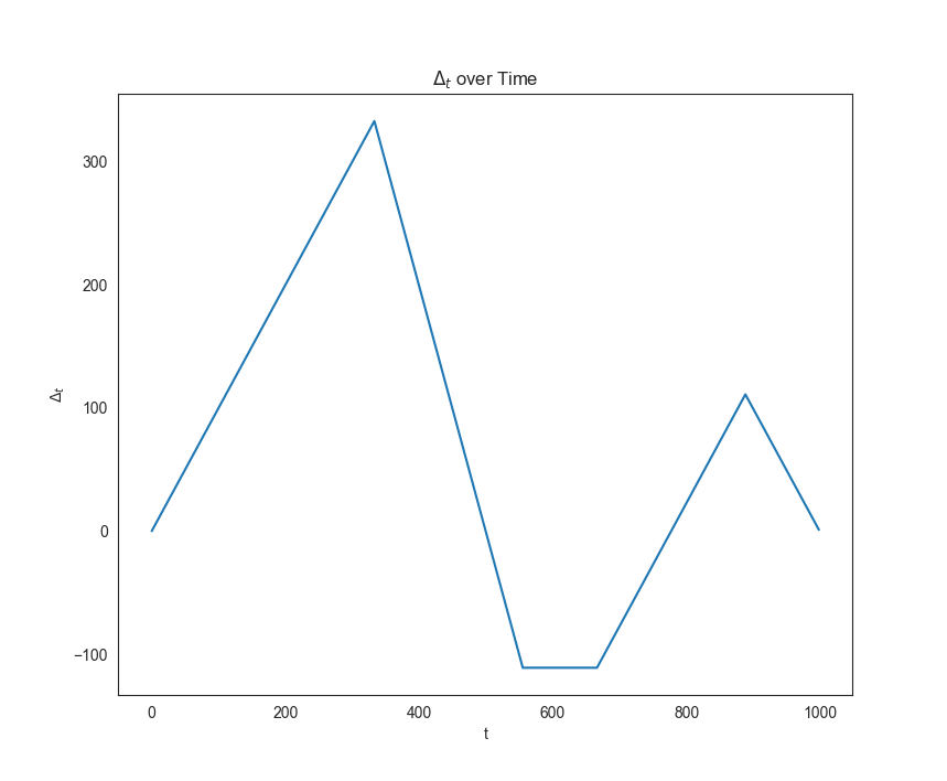
Figure 1: A plot of $\Delta_{t}$ over time, as used in Lemma 1.

We now apply Lemma 1 to prove Theorem 2.

Proof of Theorem 2.

Let $\mathbf{r}^{(M)}\in[0,1]^{2\cdot(3M)}$ be the counterexample constructed in Lemma 1, and let $N=\lfloor T/3M\rfloor$. Construct $\mathbf{r}\in[0,1]^{T}$ by concatenating $N$ copies of $\mathbf{r}^{(M)}$ and setting all other rewards to $0$ (i.e., $\mathbf{r}_{t,i}=\mathbf{r}^{(M)}_{(t\bmod 3M),i}$ for $t\leq 3MN$, $\mathbf{r}_{t,i}=0$ for $t>3MN$).

Fix any $1\leq n\leq N$, and consider the regret incurred by $\mathcal{A}$ on rounds $t\in[(n-1)\cdot 3M+1,n\cdot 3M]$ (the $n$th copy of $\mathbf{r}^{(M)}$). Since $\mathbf{r}^{(M)}$ ends with $M$ zeros, $\mathcal{A}$ will behave identically on these rounds as it would in the first $T$ rounds. Thus, by Lemma 1, $\mathcal{A}$ incurs regret at least $M/6-o(M)$ on these rounds, and at least $NM/6-o(T)$ regret in total. The per-round regret of $\mathcal{A}$ is thus at least $\mathsf{Reg}(\mathcal{A};\mathbf{r})\geq\frac{1}{T}\left(\frac{NM}{6}-o(T)\right)\geq\frac{1}{12}-o(1).$ ∎

5 Low-Regret Strongly History-Restricted Algorithms

5.1 Averaging over restarts

In the previous section, we showed that running a mean-based learning algorithm over the restricted history does not result in a low-regret strongly history-restricted learning algorithm. But are there non-mean-based algorithms which lead to low-regret strongly history-restricted algorithms? Do low-regret strongly history-restricted algorithms exist at all?

In this section, we will show that the answer to both of these questions is yes. We begin by constructing a strongly $M$-history-restricted algorithm called the AverageRestart algorithm (Algorithm 2) which incurs per-round regret of at most $O(\sqrt{(\log d)/M})$ (matching the lower bound of Theorem 3.1). Intuitively, AverageRestart randomizes over several different versions of PeriodicRestart – in particular, one can view the output of AverageRestart as first randomly sampling a starting point $s$ uniformly over the last $M$ rounds, and outputting the action that $\mathcal{A}$ would play having only seen rewards $r_{s}$ through $r_{t-1}$ (if $s\leq 0$ or $s>T$, we assume that $r_{s}=0$). Note that this algorithm is strongly $M$-history-restricted, as no step of this algorithm depends specifically on the round $t$.

0:  Time horizon $T$, history-restriction $M$, no-regret algorithm $\mathcal{A}$.

1:  for $t=0\to T$ do

2:     for $m=1\to M$ do

3:        $x_{t}^{(m)}\mathrel{\mathop{\mathchar 58\relax}}=\mathcal{A}(r_{t-m},r_{t-m+1},\dots,r_{t-1})$ (where we let $r_{t}=0$ for $t\leq 0$).

4:     end for

5:     Play action $x_{t}=\frac{1}{M}\sum_{m=1}^{M}x_{t}^{(m)}$.

6:  end for

Algorithm 2 AverageRestart

Theorem 5.1 (Average Restart Regret).

Assume the algorithm $\mathcal{A}$ has the property that $\mathsf{Reg}(\mathcal{A};\mathbf{r})\leq R(T,d)$ for any online learning instance $\mathbf{r}\in[0,1]^{T\times d}$. Then, for any instance $\mathbf{r}\in[0,1]^{T\times d}$

$$\mathsf{Reg}(\textsc{AverageRestart};\mathbf{r})\leq R(M,d).$$

Proof.

See appendix. ∎

As with PeriodicRestart, by choosing $\mathcal{A}$ to be Hedge, we obtain a strongly $M$-history-restricted algorithm with regret $O(\sqrt{(\log d)/M})$.

Corollary 2.

For any $M>0$, $d\geq 2$, there exists a strongly history-restricted algorithm $\mathcal{A}$ such that for any online learning instance $\mathbf{r}\in[0,1]^{T\times d}$, $\mathsf{Reg}(\mathcal{A};\mathbf{r})\leq O(\sqrt{(\log d)/M})$.

5.2 Averaging restarts over the entire time horizon

Earlier, we asked whether there were non-mean-based learning algorithms which give rise to strongly history-restricted learning algorithms with regret $o(1)$. While it is not immediately obvious from the description of AverageRestart, this algorithm is indeed of this form. We call the corresponding (non-history-restricted) learning algorithm AverageRestartFullHorizon (Algorithm 3). In particular, the action $x_{t}$ output by AverageRestart at time $t$ is given by

$$x_{t}=\textsc{AverageRestartFullHorizon}(r_{t-M},\dots,r_{t-1}).$$

where AverageRestartFullHorizon is initialized with time horizon $M$.

0:  Time horizon $T$, no-regret algorithm $\mathcal{A}$.

1:  for $t=0\to T$ do

2:     for $\tau=1\to T$ do

3:        $x_{t}^{(\tau)}\mathrel{\mathop{\mathchar 58\relax}}=\mathcal{A}(r_{t-\tau},r_{t-\tau+1},\dots,r_{t-1})$ (where we let $r_{t}=0$ for $t\leq 0$).

4:     end for

5:     Play action $x_{t}=\frac{1}{T}\sum_{\tau=1}^{T}x_{t}^{(\tau)}$.

6:  end for

Algorithm 3 AverageRestartFullHorizon

Interestingly, if $\mathcal{A}$ is a low-regret algorithm, so is AverageRestartFullHorizon. This follows directly from Theorem 5.1.

Theorem 3.

Assume the algorithm $\mathcal{A}$ has the property that $\mathsf{Reg}(\mathcal{A};\mathbf{r})\leq R(T,d)$ for any online learning instance $\mathbf{r}\in[0,1]^{T\times d}$. Then, for any instance $\mathbf{r}\in[0,1]^{T\times d}$

$$\mathsf{Reg}(\textsc{AverageRestartFullHorizon};\mathbf{r})\leq R(T,d).$$

Proof.

Set $M=T$ in the proof of Theorem 5.1. (In particular, the proof of Theorem 5.1 applies for any choice of $M$ and $T$, not only $T\gg M$). ∎

6 Simulations

6.1 Experiment Setup

We conduct some experiments to assess the performance of the history-restricted algorithms we introduce in some simple settings. In particular, we consider Algorithms 1,  2,  3, and an $M$-history-restricted mean-based algorithm, all applied to the Multiplicative Weights Update algorithm with fixed learning rate $\eta=1/2$. We also compare to classic Multiplicative Weights algorithm, which is known to have favorable performance compared to Multiplicative Weights in various non-worst-case settings (though it has linear regret in general) (De Rooij et al., 2014). We assess performance on periodic drifting rewards (see the appendix for full details), as well as an adversarial setting for the mean-based history-restricted algorithm. The drifting rewards are parameterized by how slowly their rewards change – we expect history-restricted algorithms to outperform full-horizon approaches in some cases since when the reward function for the arms changes quickly, it is more advantageous to only use more recent memory. We evaluate the algorithms by the total regret measure.

6.2 Results

The key takeaways from the results are as follows:

1. For all of our drifting reward settings, our proposed average restart and periodic restart methods (Algorithms 1 and  2) outperform or are on par with the other methods.

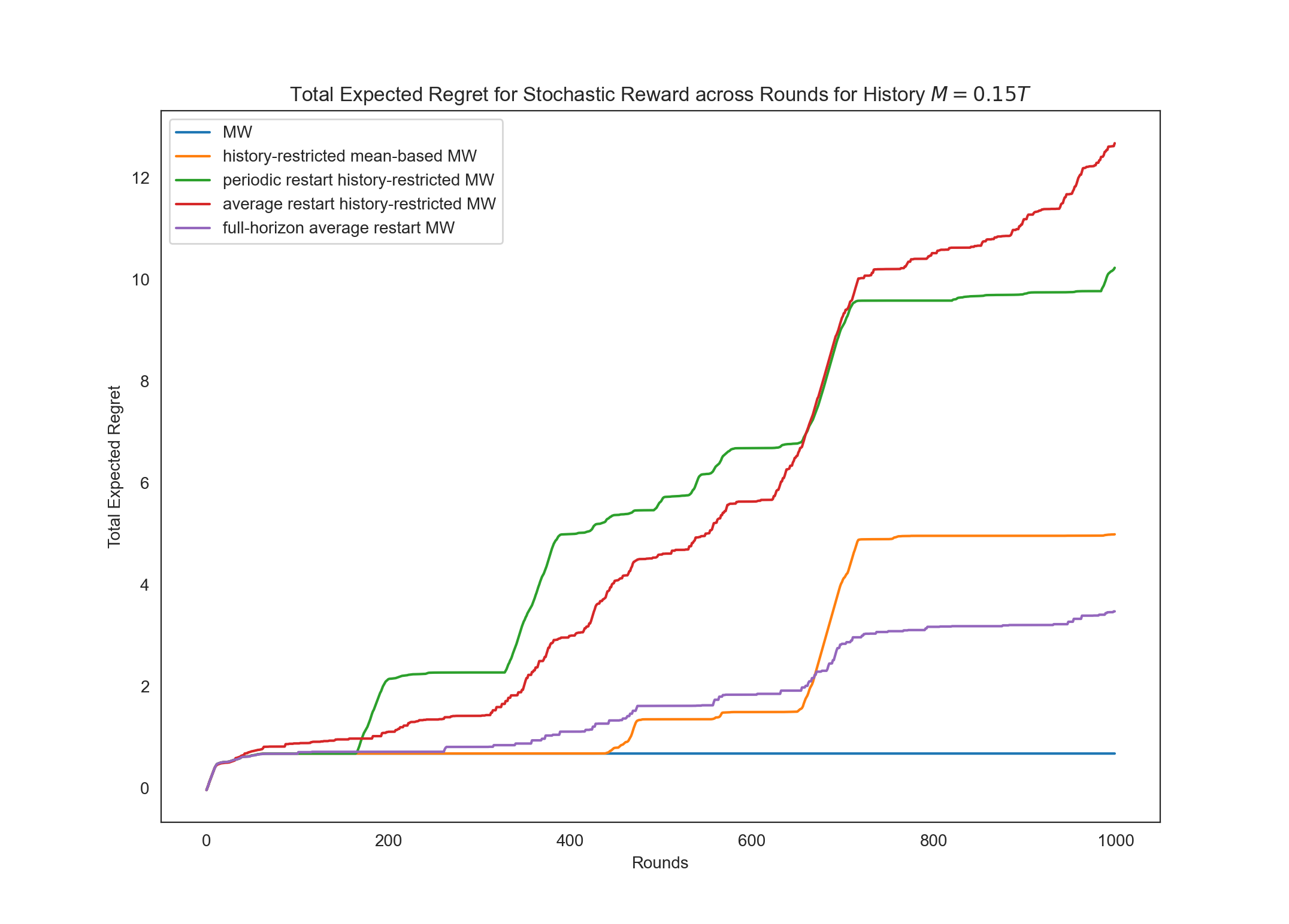
Figure 5: We plot the total regret of the algorithms over time for the stochastic rewards case – observe that in this case, Multiplicative Weights outperforms the history-restricted methods, which makes sense since the reward distribution is stationary.

2. In the stochastic setting, MW outperforms our proposed methods, though the difference is small (Figure 5 in Section C).

3. In the adversarial setting constructed in Lemma 1, the no-regret history-restricted methods outperform the other algorithms, and the mean-based history-restricted method attains far worse regret, as our theory proves (Figure 2 (b)).

4. Our history-restricted algorithms are highly sensitive to periodicity in the online rewards, and as hypothesized, can take advantage of periodicity that corresponds to the history parameter $M$. See Section D of the appendix for a thorough study of the impact of $M$ on performance.

5. Remarkably, Algorithm 3, our full-horizon variant of the average restart algorithm, can outperform Multiplicative Weights in various drifting settings, suggesting it is an interesting algorithm in its own right from an average case perspective.

6. We also remark that in the results presented in this section, it may appear that the periodic restart method (Algorithm 1) is strictly better than the average restart (Algorithm 2). This supposition tends to be true for small $M$, but is not necessarily the case when $M$ is larger – see the appendix for a discussion and ablations across the value of $M$.

The full results are in the appendix (Sections C and  D). Here we present a few figures which demonstrate the main points. Figure  2 highlights the improved average case performance of our history-restricted algorithms – the periodic and average restart history-restricted methods (Algorithms 1 and  2) are particularly good, and perhaps surprisingly, the full-horizon average restart algorithm (Algorithm 3) can sometimes outperform Multiplicative Weights (though on average over high-frequency drifting rewards it performs on par). Figure 2 validates our theoretical conclusions, and also demonstrates that the no-regret history-restricted algorithms perform very well in comparison to Multiplicative Weights on the hard example for history-restricted mean-based learners.

(a) Left

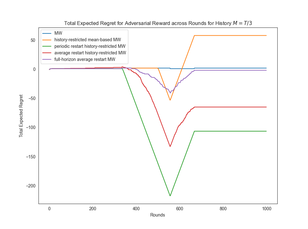
(b) Right

Figure 2: (Left) We plot the total regret of the algorithms over time over a uniform average of high-frequency drifting scenarios where the periods of the mean reward of arm $1$ are $T/20,T/10,T/5,$ and $T/2$ and arm $2$ flips an unbiased coin for reward $\{\pm 1\}$ – the history-restricted algorithms significantly outperform the classic no-regret algorithms. (Right) We plot the total regret of the algorithms over time for one block of the adversarial rewards case (see the construction in Lemma 1) – observe that the mean-based history-restricted learner attains regret on order $M/6$ (here, $M=T/3$), while our no-regret history-restricted learners all outperform Multiplicative Weights.

7 Conclusion and Future Work

In this paper, we initiated the study of history-restricted online learning and produced novel history-restricted no-regret algorithms, as well as provided linear regret lower bounds against a natural class of history-restricted learners.

There are many avenues for future work: 1) It would be interesting to consider history-restricted extensions to other notions of regret (e.g., swap regret (Blum and Mansour, 2007a)); 2) Our strongly-history-restricted algorithms are more computationally demanding than other no-regret algorithms – understanding the computational limitations of these methods would be useful as well; 3) Obtaining a theoretical characterization of performance improvements for history-restricted methods relative to classic online learners in general non-stationary settings would be quite interesting as well.

Appendix A Related Work

A.1 Adaptive Multiplicative Weights

There is a lot of existing work on understanding the behavior of Multiplicative Weights under various non-adversarial assumptions and properties of the loss sequence (Cesa-Bianchi et al., 2007; Hazan and Kale, 2010), as well as on coming up with adaptive algorithms which perform better than Multiplicative Weights in both worst-case and average-case settings (Erven et al., 2011; De Rooij et al., 2014; Koolen et al., 2016; Mourtada and Gaïffas, 2019). There is a particular emphasis on trading off between favorable performance for Follow-the-Leader and Multiplicative Weights in various average case settings. Our work connects to this literature by introducing history-restricted algorithms which empirically outperform both MW and FTL for a class of drifting and periodic rewards.

A.2 Private Learning and Discarding Data

History-restricted online learning algorithms can be viewed as private with respect to data sufficiently far in the past – such data is not taken into account in the prediction. This approach to achieving privacy is similar in principle to federated learning (Kairouz et al., 2021), which ensures that by decentralizing the data store, many parties participating in the model training will simply never come into contact with certain raw data points, thus mitigating privacy risks. Similarly, history-restricted approaches also provide an alternate angle on privacy-preserving ML systems which must store increasing amounts of streaming data (and thereby must adaptively set their privacy costs to avoid running out of privacy budget, see Lécuyer et al. (2019)). Additionally, the history-restricted approach to privacy yields algorithms for which data deletion (Ginart et al., 2019) is efficient – thereby ensuring “the right to be forgotten.”

A.3 Shifting Data Distributions

History-restricted algorithms are a natural approach to online learning over non-stationary time series, which is a common problem in practical industry settings (Huyen, 2022) and which has been studied for many years (Sugiyama and Kawanabe, 2012; Wiles et al., 2021; Wu, 2021; Rabanser et al., 2019). In particular, one can view history-restricted online learners as adapting to non-stationary structure in the data – thus, one may not need to go through the whole process of detecting a distribution shift and then deciding to re-train – ideally the learning algorithm is adaptive and automatically takes such eventualities into account. Our proposed history-restricted methods are one step in this direction.

Appendix B Omitted Proofs

See 3.1

Proof.

Our hard example is simple: we make use of standard hard examples used in regret lower bounds for the classical online learning setting (see e.g. Roughgarden (2016)), and simply append to such an example of length $M$ a block of $M$ $0$ rewards for all actions (effectively resetting the internal state of any history-restricted algorithm, and resulting in $0$ regret during that block). This trick allows us to only consider the regret on blocks of size $M$, and since the blocks are repeated, each block has the same best action in hindsight. Then taking the full block of length $2M$ together, we get an average regret lower bound for each block of size $\frac{1}{2}\Omega(\sqrt{M\log d})$. Adding up the regret lower bounds, we get a total regret lower bound for any history-restricted online learning algorithm with past window of size $M$ to be $\Omega\left(\frac{T}{2M}\cdot\sqrt{M\log d}\right)=\Omega\left(\sqrt{\frac{T^{2}\log d}{M}}\right)$, or $\Omega\left(\sqrt{\frac{\log d}{M}}\right)$ on average, as desired. ∎

See 5.1

Proof.

Intuitively, we will decompose the output of AverageRestart as a uniform combination of $M$ copies of PeriodicRestart (one for each offset modulo $M$ of reset location); since PeriodicRestart has per-round regret $R(M,d)$, so will AverageRestart.

Let $i^{*}=\arg\max_{i\in[d]}\sum_{t}r_{t,i}$. For any $t\in[-(M-1),T-1]$ and $m\in[M]$, let $y_{t}^{(m)}=x_{t+m}^{(m)}=\mathcal{A}(r_{t},r_{t+1},\dots,r_{t+m-1})$. Now, note that

$$\sum_{t=1}^{T}\langle x_{t},r_{t}\rangle = \sum_{t=1}^{T}\frac{1}{M}\sum_{m=1}^{M}\langle x_{t}^{(m)},r_{t}\rangle$$

$$= \sum_{t=1}^{T}\frac{1}{M}\sum_{m=1}^{M}\langle y_{t-m}^{(m)},r_{t}\rangle$$

$$= \sum_{t^{\prime}=-M+1}^{T-1}\frac{1}{M}\sum_{m=1}^{M}\langle y_{t^{\prime}}^{(m)},r_{t^{\prime}+m}\rangle$$

$$= \sum_{t^{\prime}=-M+1}^{T-1}\frac{1}{M}\sum_{m=1}^{M}\langle\mathcal{A}(r_{t^{\prime}},r_{t^{\prime}+1},\dots,r_{t^{\prime}+m-1}),r_{t^{\prime}+m}\rangle$$

$$\geq \sum_{t^{\prime}=-M+1}^{T-1}\frac{1}{M}\left(\sum_{m=1}^{M}r_{t^{\prime}+m,i^{*}}-M\cdot R(M,d)\right)$$

$$= \left(\sum_{t=1}^{T}r_{t,i^{*}}\right)-(T+M)R(M,d).$$

Here we have twice used the fact that $r_{s}=0$ for $s\leq 0$ and $s>T$; once for rewriting the sum in $t$ in terms of $t^{\prime}$ (the terms that do not appear in the original sum have $t^{\prime}+m\not\in[1,T]$, so the inner product evaluates to $0$), and once again when we rewrite the sum in $t^{\prime}$ in terms of $T$ (each $r_{t,i}$ for $1\leq t\leq T$ appears exactly $M$ times; other $r_{t,i}$ for $t\not\in[1,T]$ appear a variable number of times, but they all equal $0$). Since $M\leq T$, it follows that $\mathsf{Reg}(\textsc{AverageRestart};\mathbf{r})\leq R(M,d)$. ∎

Appendix C Additional Simulation Results

In the following plots, we compute the total expected regret as a function of time for the various online learning algorithms on the various reward sequences. Since the stochastic behavior is known to us (as we simulate it), we directly compute the expected rewards analytically, though we run the algorithms on stochastically sampled rewards. For each fixed reward sequence, we run each algorithm $3$ times and average the results (since some of the algorithmic behavior is random).

C.1 Further Details of the Simulation Methodology

We consider the following settings over $T=1000$ rounds, all with two arms which correspond to a coin flip with some bias $p$ between reward $+1$ and reward $-1$:

1. The stochastic i.i.d. setting where arm $1$ outputs $+1$ with probability $1/2+1/\sqrt{T}$ and arm $2$ outputs $+1$ with probability $1/2$.

2. Several drifting settings where arm $1$ outputs $+1$ with probability $|\sin\left(\pi/6+t\cdot\pi/\varphi\right)|$ at time $t\in[T]$. Here $\varphi$ is the period of the oscillation. See Figure 3 for some examples. We let arm $2$ output $+1$ with probability $1/2$.

3. Several pairwise drifting settings where arm $1$ outputs $+1$ with probability $|\sin\left(\pi/6+t\cdot\pi/\varphi_{1}\right)|$ at time $t\in[T]$ and arm $2$ outputs $+1$ with probability $|\sin\left(\pi/6+t\cdot\pi/\varphi_{2}\right)|$.

4. A random walk setting where the probability $p$ that arm $1$ outputs $+1$ drifts according to $p_{t+1}=p_{t}+Z_{t}$, where $Z_{t}$ are i.i.d. Gaussians $\mathcal{N}(0,\sigma^{2})$ for variance parameter $\sigma^{2}$. If $p_{t}+Z_{t}>1$ or $p_{t}+Z_{t}<0$, we cap the result $p_{t+1}=1$ or $p_{t+1}=0$ respectively. Arm $2$ outputs $+1$ with probability $1/2$. In our experiments, we sample $3$ random walk instances for each choice of $\sigma$ and display results for all three.

5. The hard case for mean-based history-restricted algorithms with $M=T/3$ (see Lemma 1).

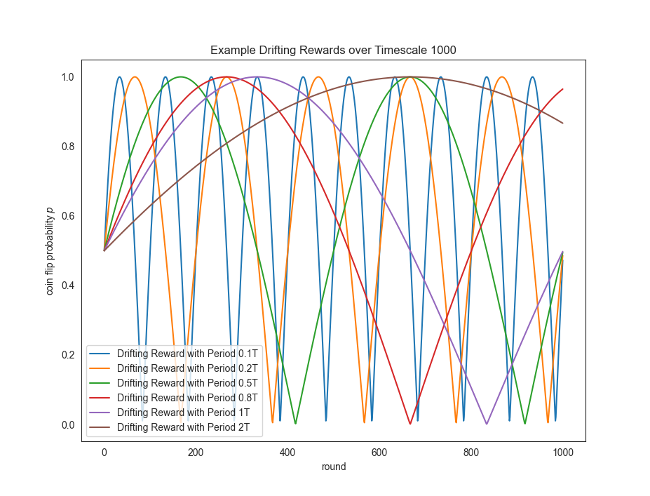
Figure 3: The drifting rewards used in our simulations are all defined over $\{\pm 1\}$ and are parameterized by the probability $p^{(t)}$ of getting heads for each arm as a function of time.

Notably, these drifting rewards are parameterized by how slowly their rewards change – we expect history-restricted algorithms to outperform full-horizon approaches in some cases since when the reward function for the arms changes quickly, it is more advantageous to only use more recent memory. We evaluate the algorithms by the total regret measure.

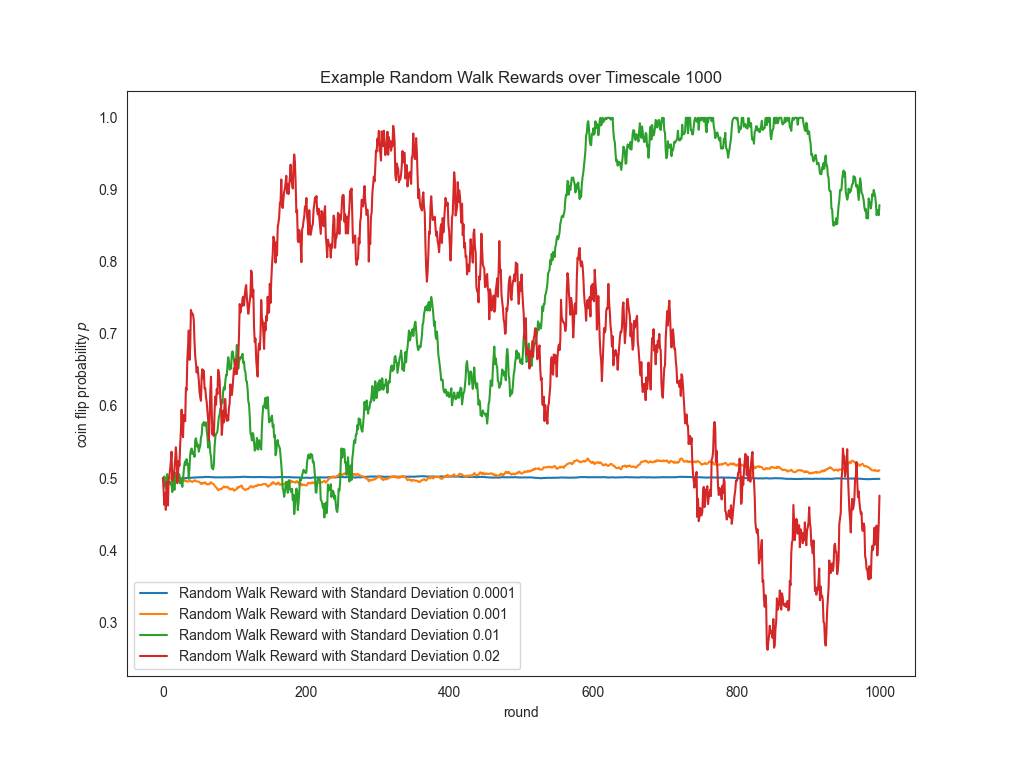
Figure 4: The random walk rewards used in our simulations are parameterized by the variance parameter $\sigma^{2}$ that governs the distribution the update to the current probability $p^{(t)}$ of getting heads for each arm as a function of time.

We also specify the specific form of the history-restricted mean-based MW algorithm:

0:  Reward sequence $\{r_{t}\}_{t=1}^{T}$ for $r_{t}\in\mathbb{R}^{d}$ corresponding to $d$ arms; memory $M\leq T$; learning rate $\eta$

1:  Initialize $w_{0}=[1,\cdots,1]\in\mathbb{R}^{d}$.

2:  for $t=0\to M-1$ do

3:     Sample action $a_{t}$ according to $\left[\frac{w_{t}(i)}{\sum_{j=1}^{d}w_{t}(j)}\right]_{i=1}^{d}$ and experience loss $r_{t}$

4:     $w_{t+1}=\left(1+\eta r_{t}\right)\odot w_{t}$

5:  end for

6:  for $t=M\to T$ do

7:     Sample action $a_{t}$ according to $\left[\frac{w_{t}(i)}{\sum_{j=1}^{d}w_{t}(j)}\right]_{i=1}^{d}$ and experience loss $r_{t}$

8:     $w_{t+1}=\frac{\left(1+\eta r_{t}\right)}{\left(1+\eta r_{t-M}\right)}\odot w_{t}$

9:  end for

Algorithm 4 History-Restricted Multiplicative Weights

For ease of reading the plots, we also include a map between the algorithm and the color of its performance graphs in the plots below:

1. Multiplicative Weights (MW): Blue

2. History-Restricted Periodic Restart (Algorithm 1): Green

3. History-Restricted Average Restart (Algorithm 2): Red

4. Full-Horizon Average Restart (Algorithm  3): Purple

5. History-Restricted Mean-Based (Algorithm 4): Orange

C.2 Total Regret vs. Rounds

In the following plots, we compute the total expected regret as a function of time for the various online learning algorithms on the various reward sequences. Since the stochastic behavior is known to us (as we simulate it), we directly compute the expected rewards analytically, though we run the algorithms on stochastically sampled rewards. For each fixed reward sequence, we run each algorithm $3$ times and average the results (since some of the algorithmic behavior is random).

We make the following observations:

1. There appear to be two qualitative modes of behavior: “stochastic” and “periodic”: In the stochastic mode, our history-restricted algorithms tend to perform linearly worse over time compared to Multiplicative Weights, but the gap is relatively small (even for the mean-based history-restricted algorithm, which is not no regret in general). See the random walk rewards for small $\sigma$, as well as the periodic rewards for either very small or very large $\varphi$ for examples of the stochastic mode. In the periodic mode (which includes various examples from the periodic rewards and the random walk rewards, for appropriate choices of period and (typically larger) standard deviations), the total regret over time tends to stay flat for a period of time before rapidly becoming negative for the history-restricted methods (and the full-horizon average restart method) – Multiplicative Weights, on the other hand, is relatively flat at $0$ regret through all of time. See the random walk rewards for larger $\sigma$ as well as the periodic rewards for medium sized $\varphi$ and the paired periodic rewards where $\varphi_{1}$ and $\varphi_{2}$ are close together for examples of the periodic mode.

2. The history-restricted mean-based algorithm, despite not being a no-regret algorithm, does relatively well in the periodic settings – however, this algorithm is prone to large spikes in regret compared to the other methods, suggesting that the worst case instances for this type of algorithm may be present in relatively simple periodic reward settings.

3. Generally, the periodic restart algorithm is much less stable compared to the average restart algorithms in its fluctuation in total regret over time. However, it is not as unstable as the history-restricted mean-based algorithm, possibly because the periodic restart algorithm is actually a no-regret algorithm.

C.2.1 Stochastic Rewards

C.2.2 Random Walk Rewards

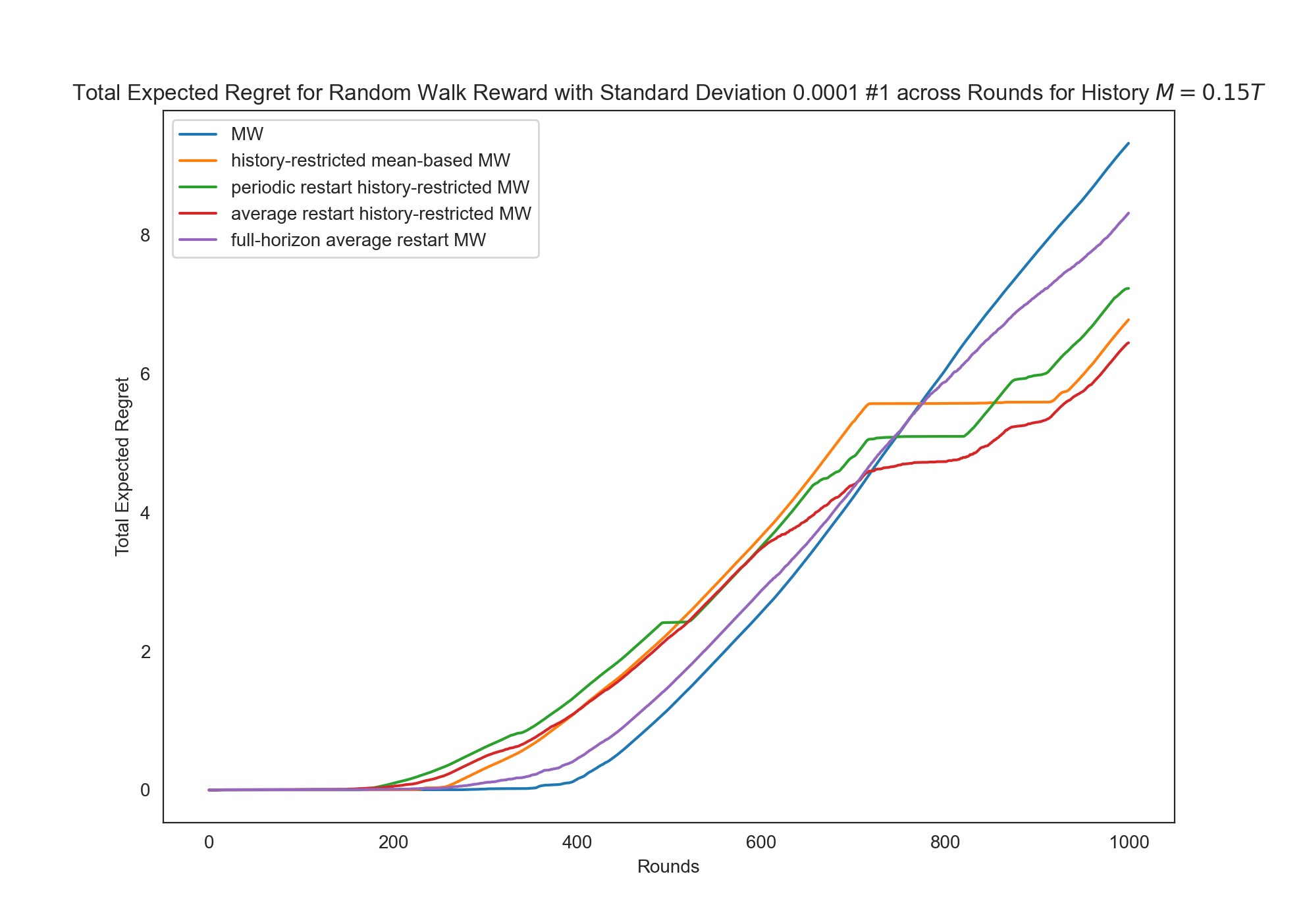
(a) Random Walk $\#1$

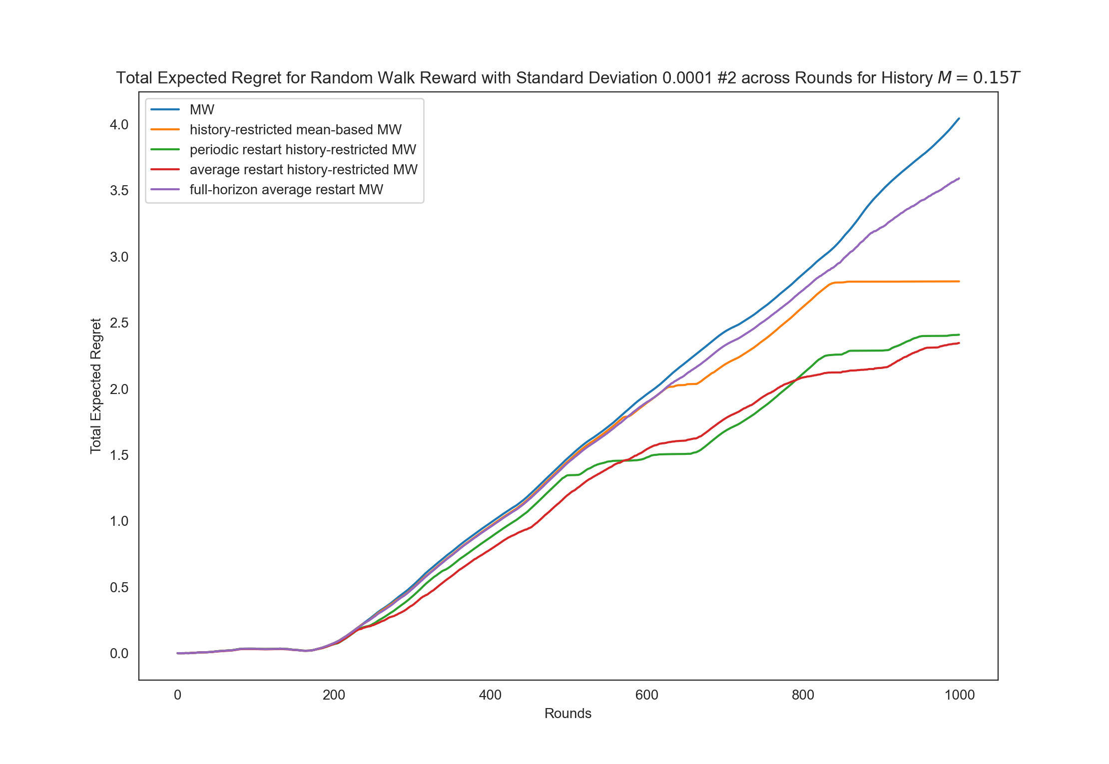
(b) Random Walk $\#2$

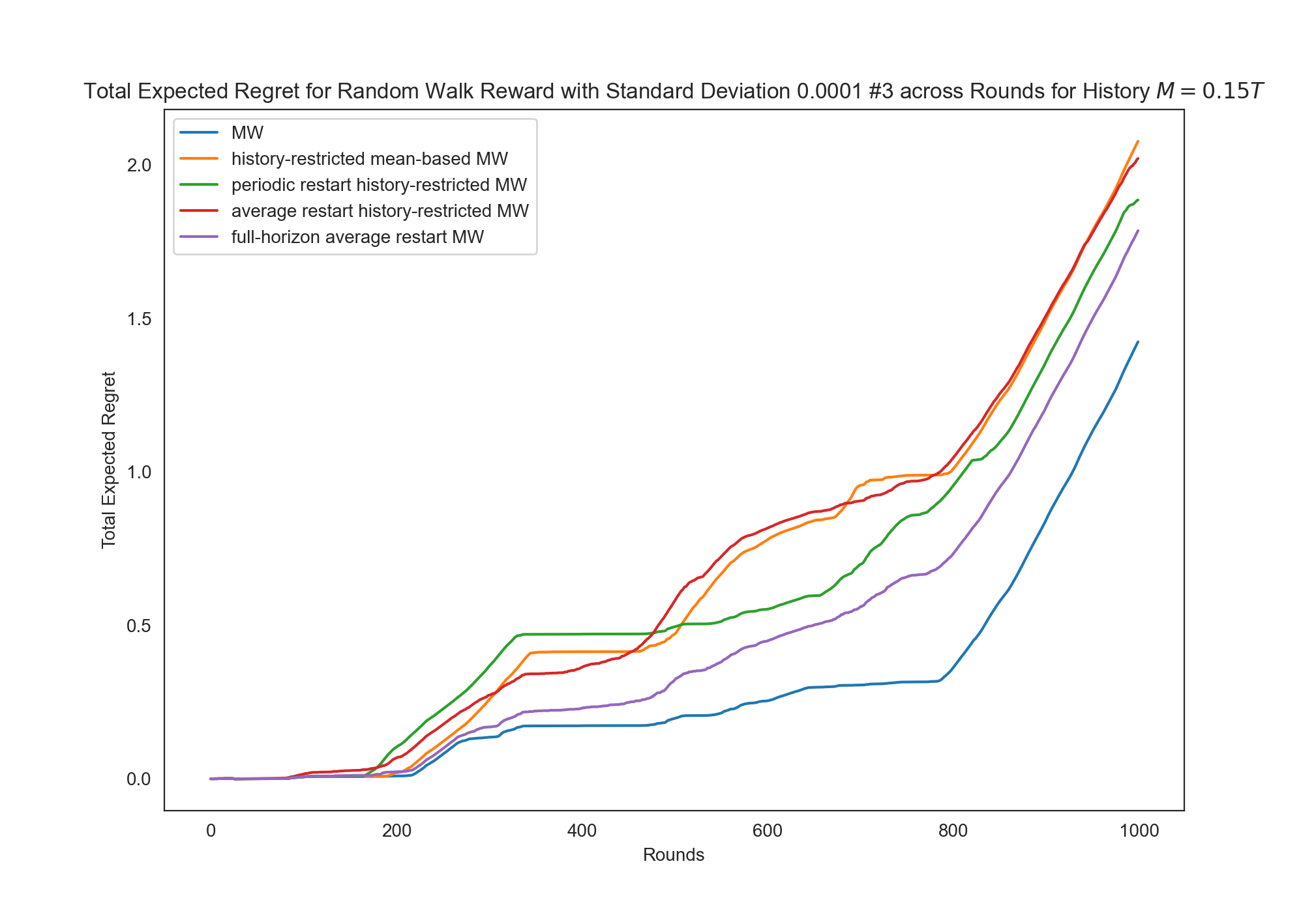
(c) Random Walk $\#3$

Figure 6: We plot the total regret of the algorithms over time for the random walk scenario with $\sigma=0.0001$.

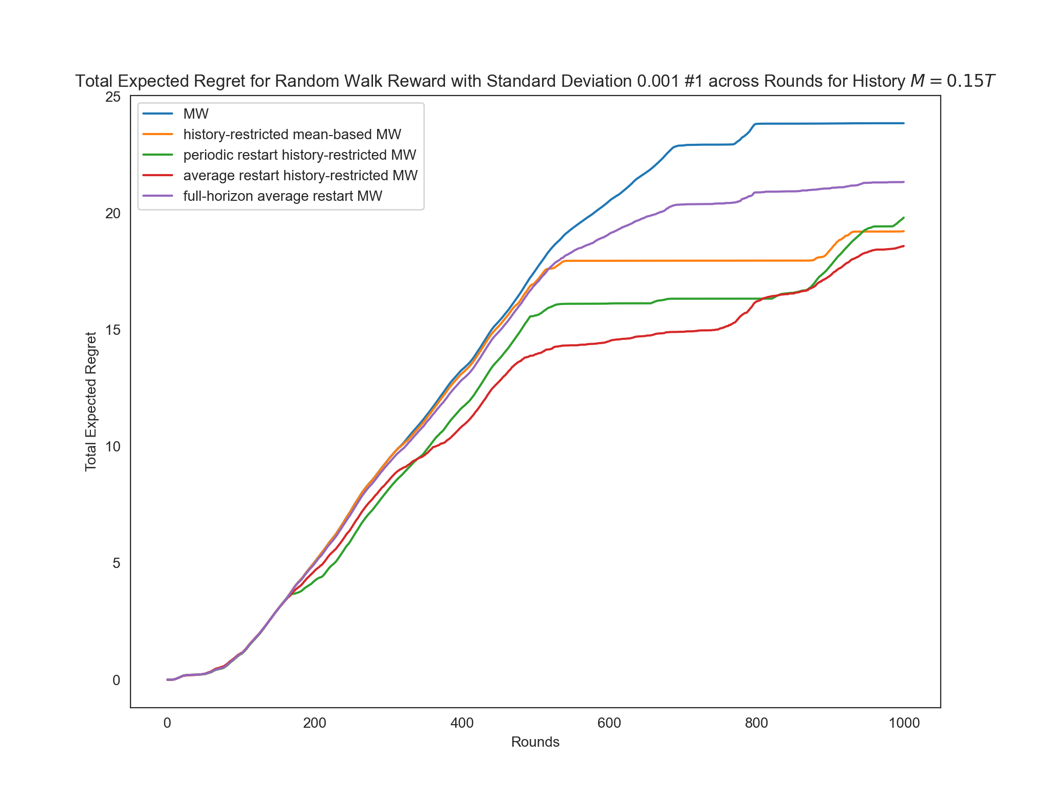
(a) Random Walk $\#1$

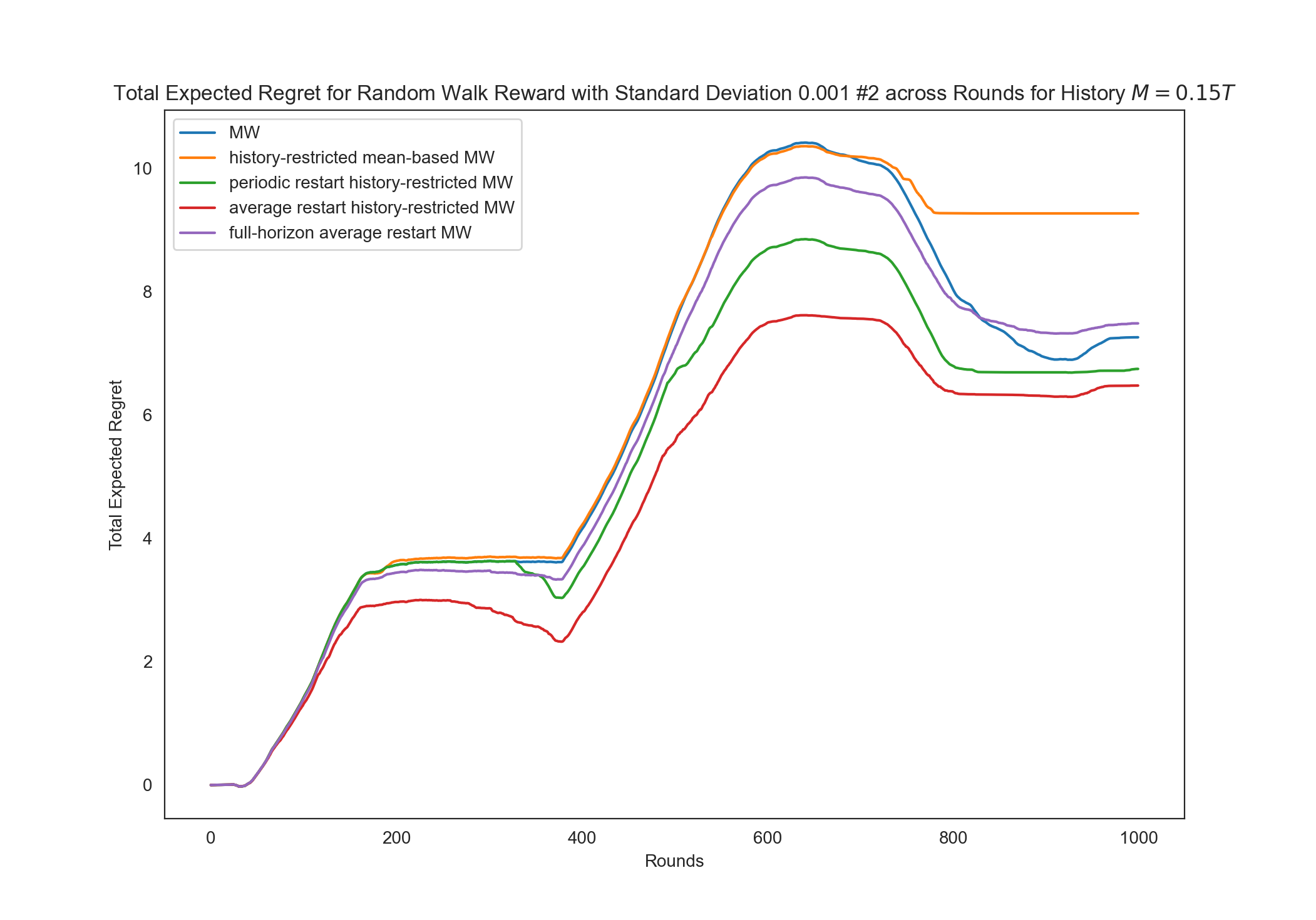
(b) Random Walk $\#2$

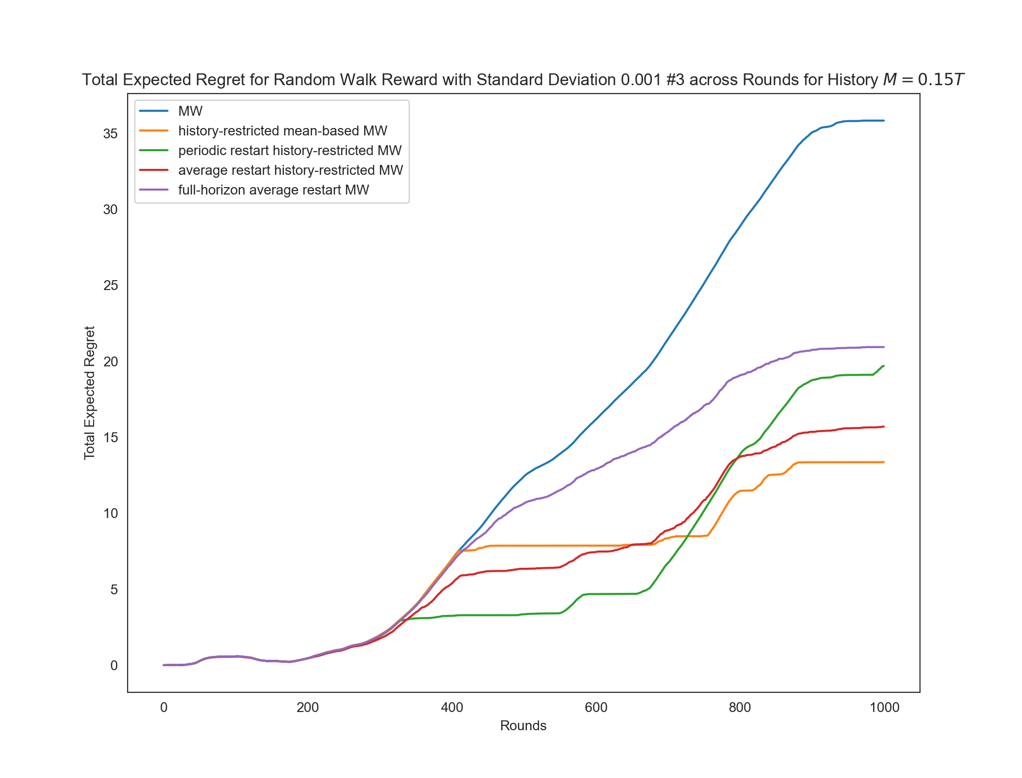
(c) Random Walk $\#3$

Figure 7: We plot the total regret of the algorithms over time for the random walk scenario with $\sigma=0.001$.

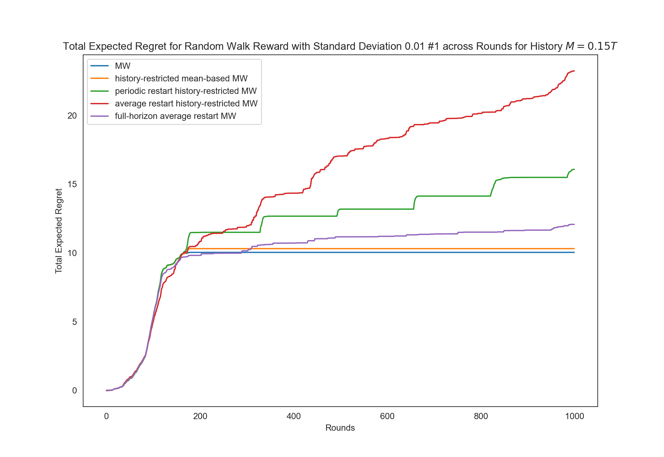
(a) Random Walk $\#1$

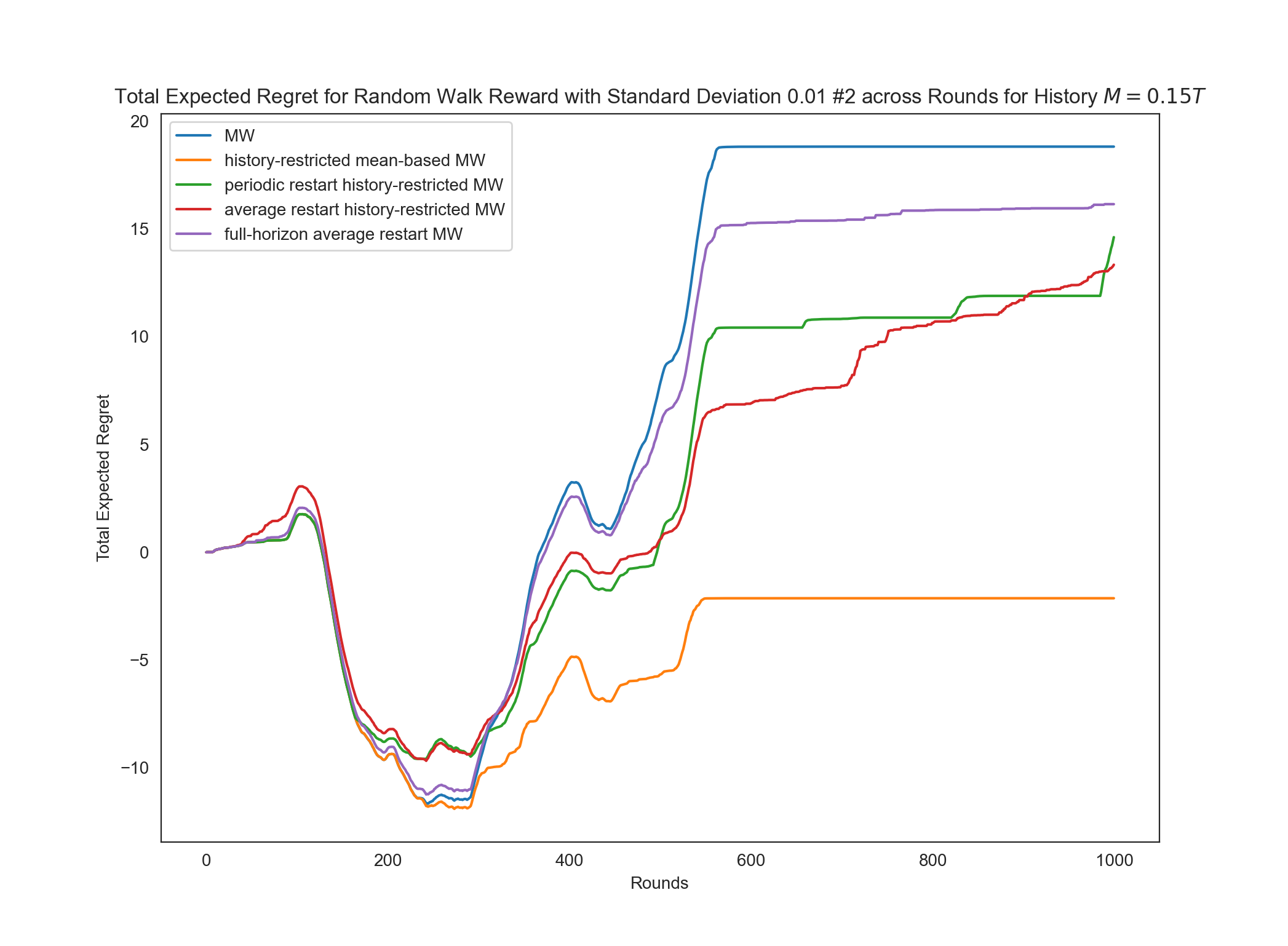
(b) Random Walk $\#2$

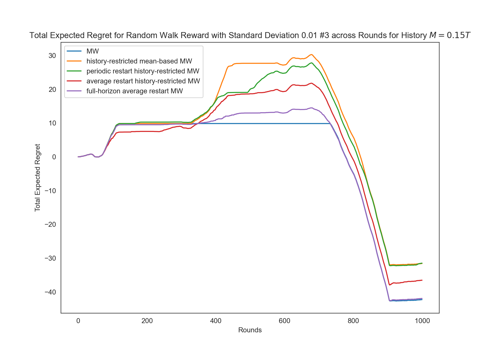
(c) Random Walk $\#3$

Figure 8: We plot the total regret of the algorithms over time for the random walk scenario with $\sigma=0.01$.

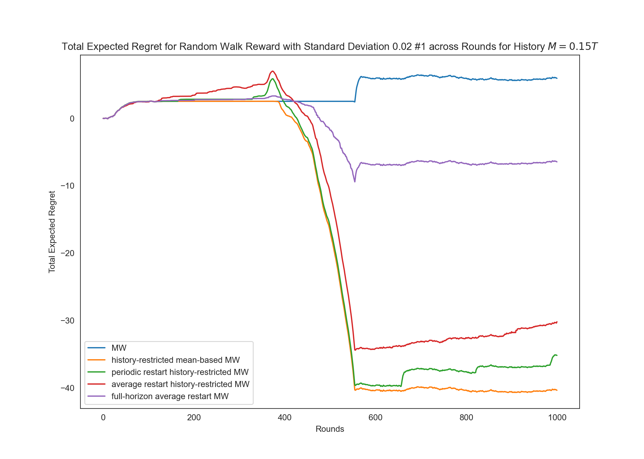
(a) Random Walk $\#1$

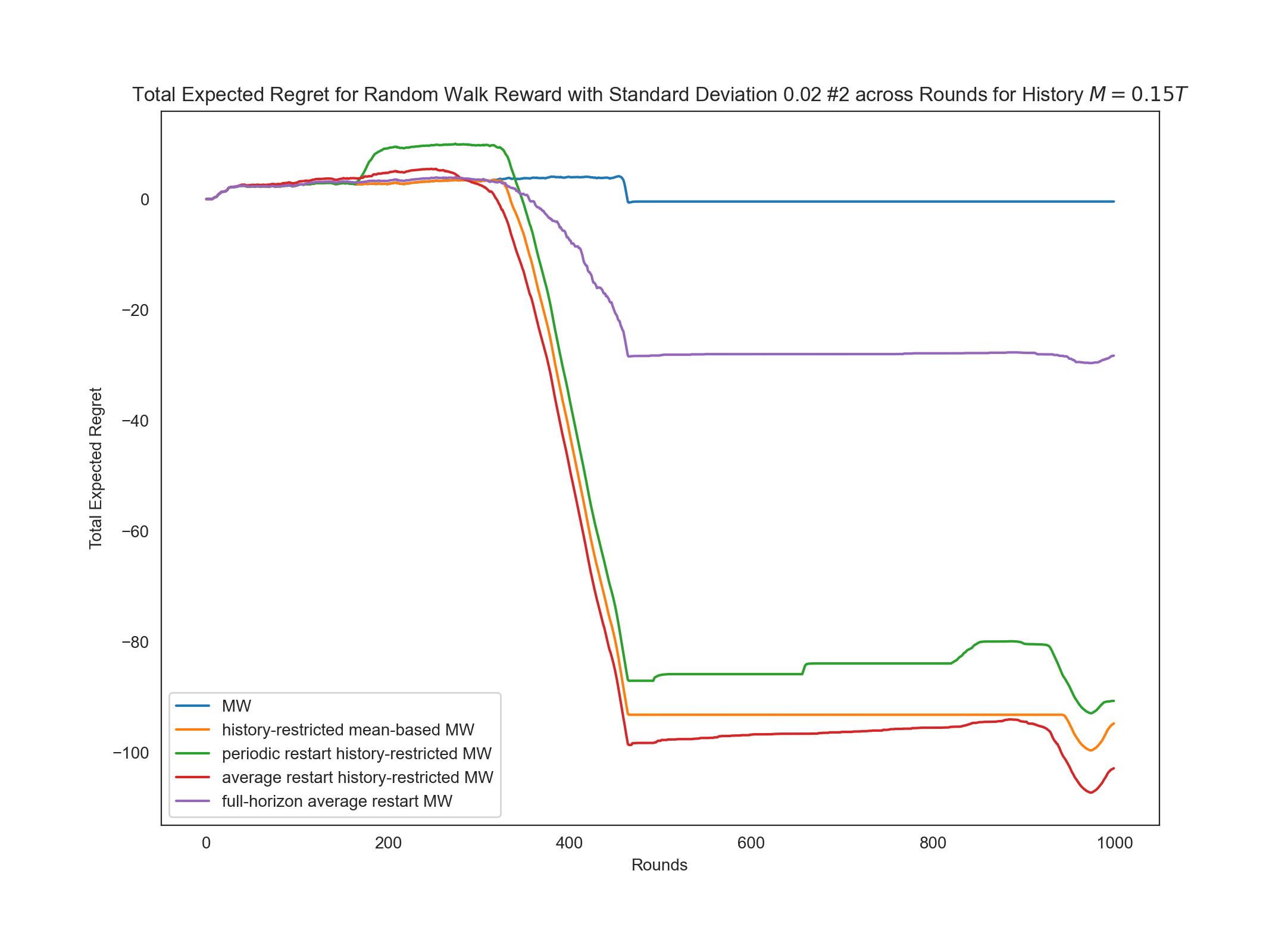
(b) Random Walk $\#2$

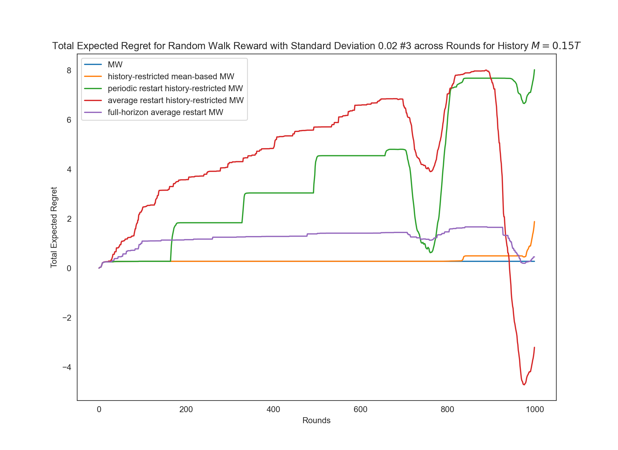
(c) Random Walk $\#3$

Figure 9: We plot the total regret of the algorithms over time for the random walk scenario with $\sigma=0.02$.

C.2.3 Periodic Rewards

For the drifting scenarios where arm $2$ is stochastic, we observe that as the period $\varphi$ decreases (e.g., the coin flip probability $p_{t}$ is high-frequency for arm $1$), the total expected regret portrait approaches the pure stochastic example.

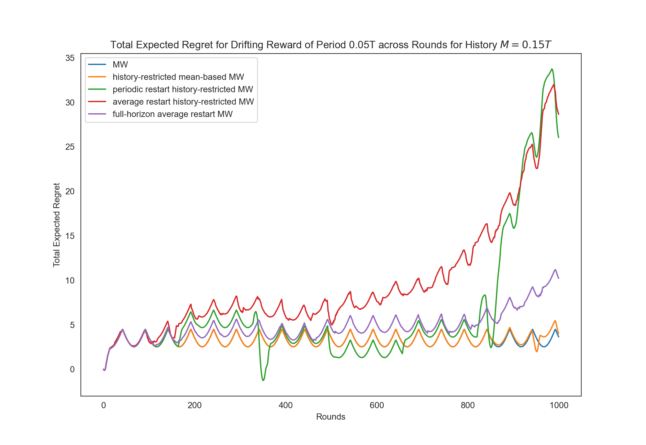
(a) $\varphi=T/20$.

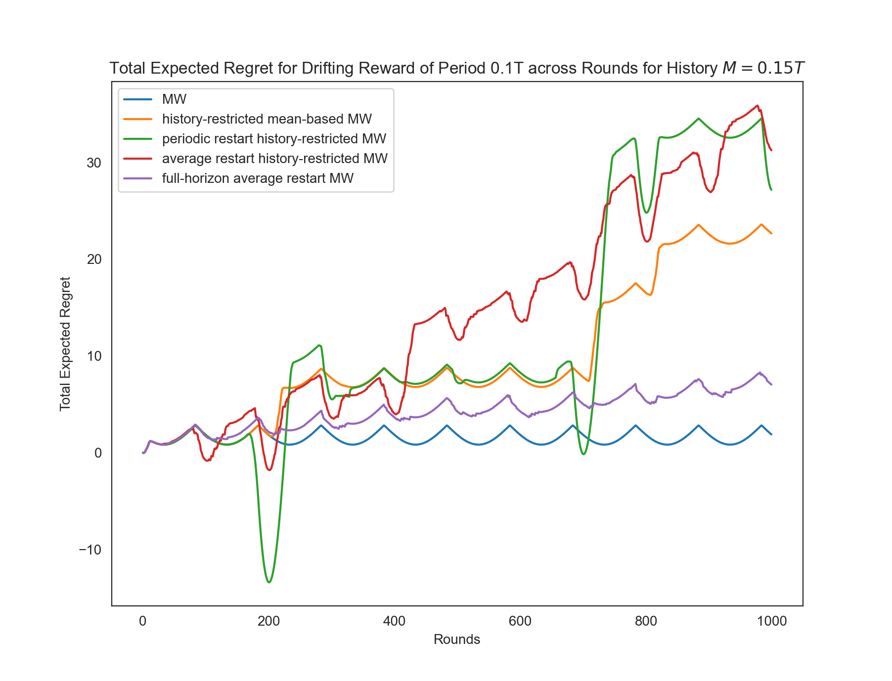
(b) $\varphi=T/10$.

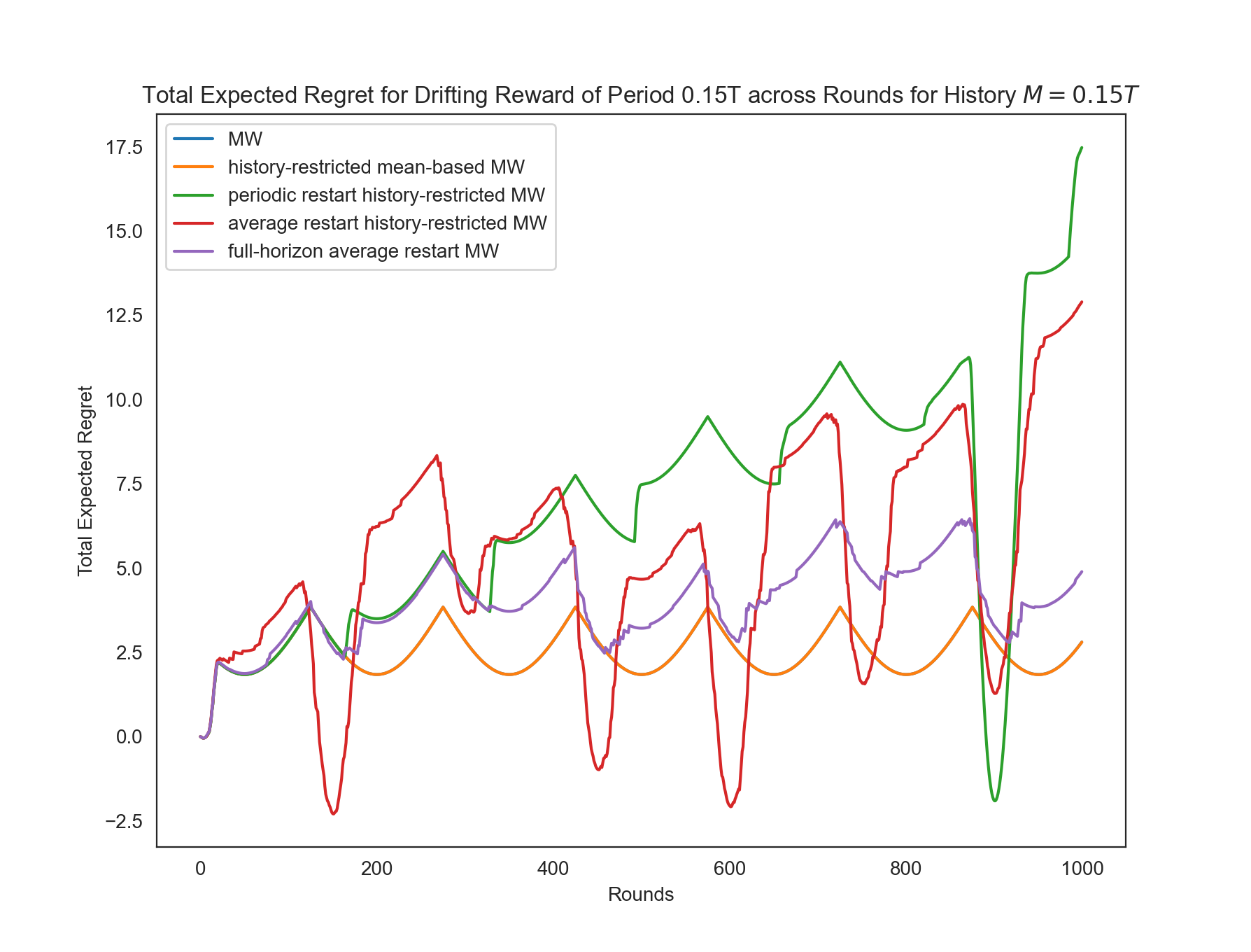
(c) $\varphi=0.15T$.

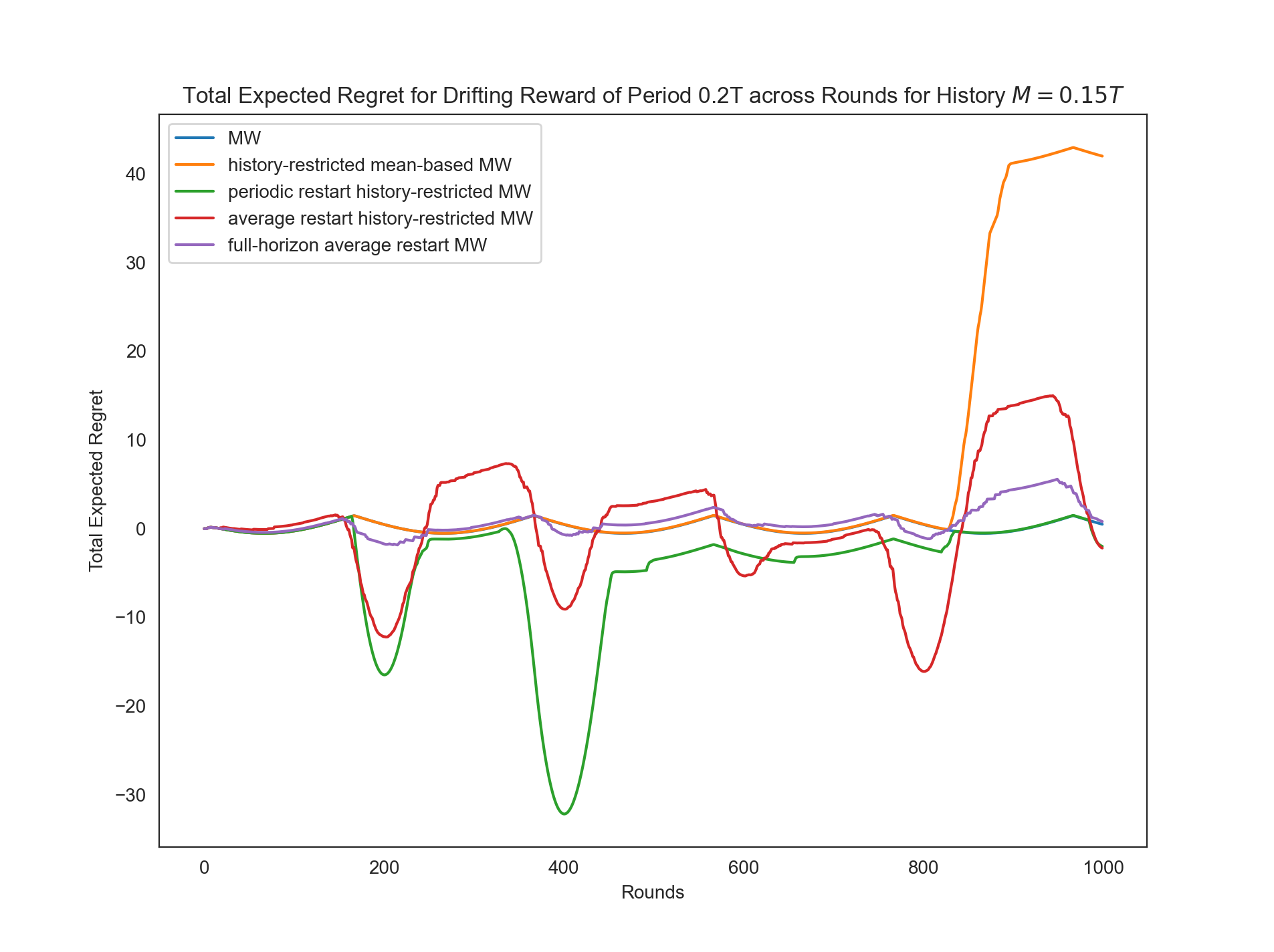
(d) $\varphi=T/5$.

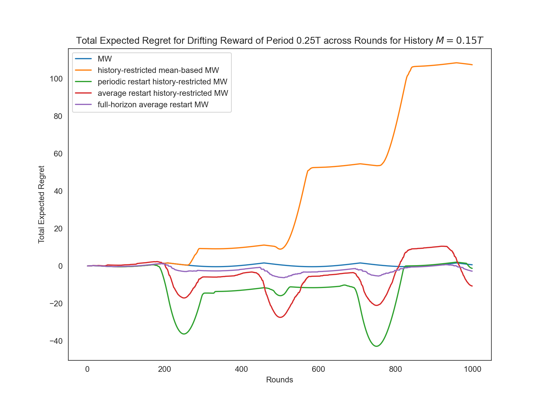
(e) $\varphi=T/4$.

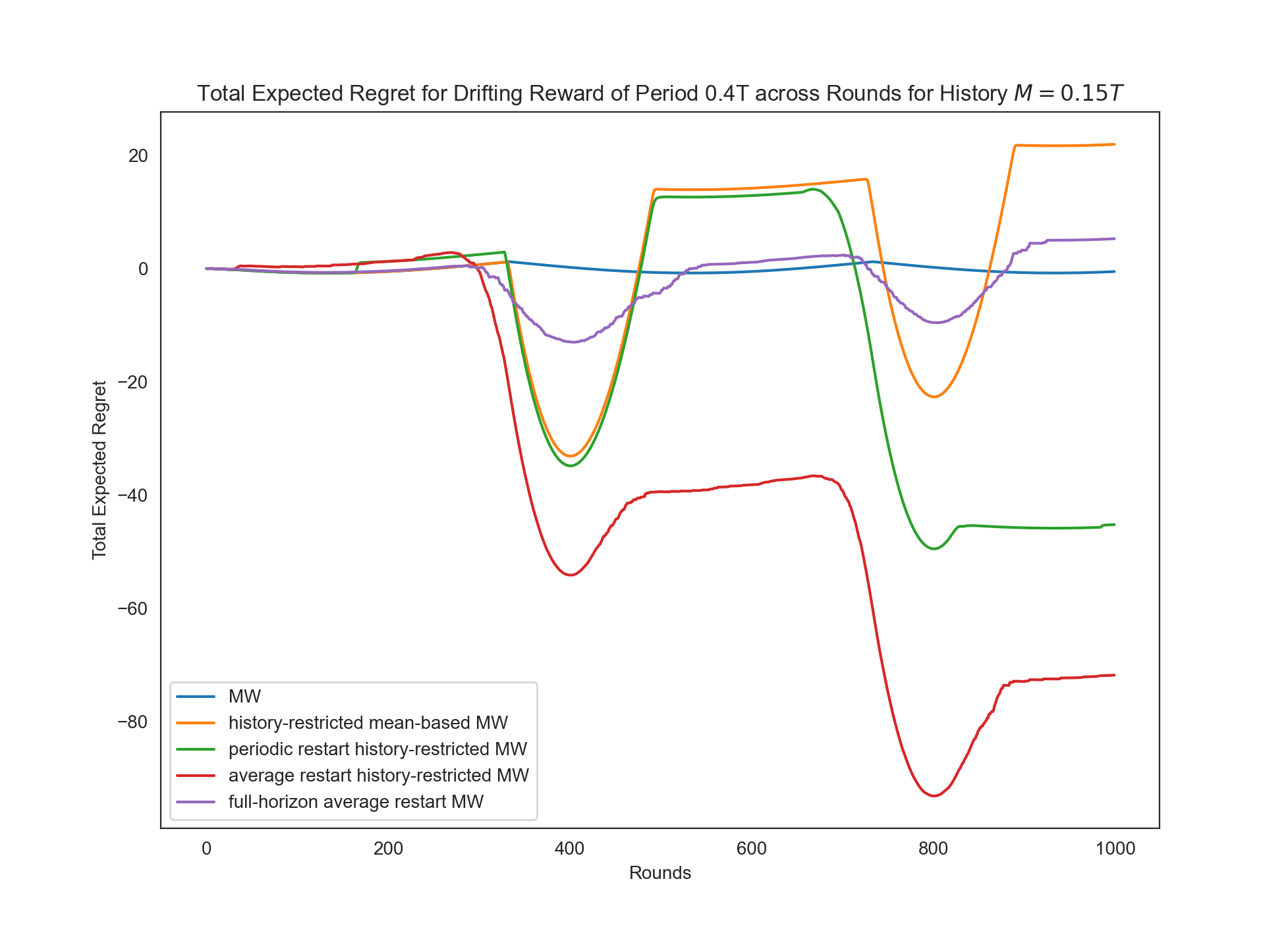
(f) $\varphi=2T/5$.

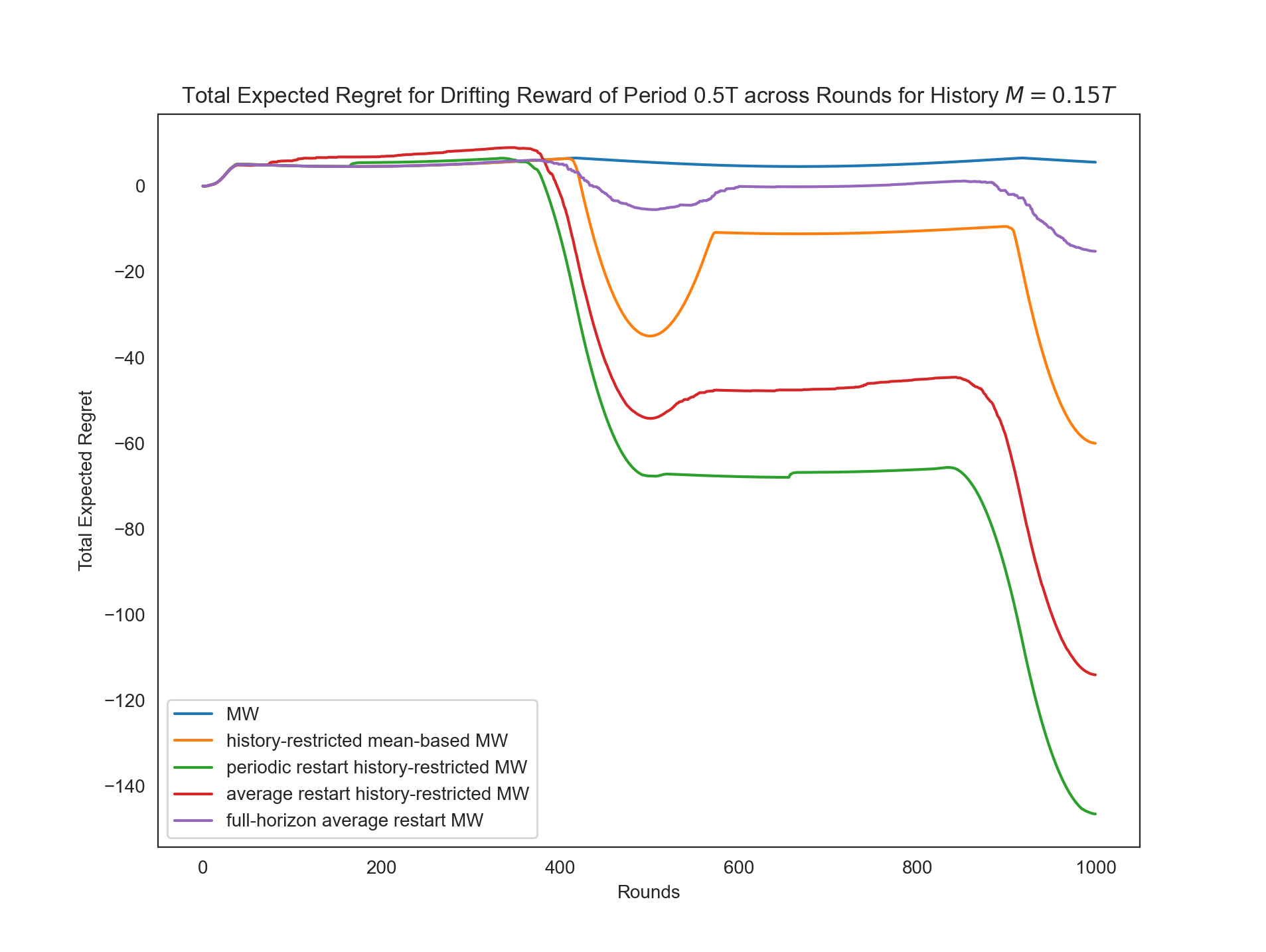
(g) $\varphi=T/2$.

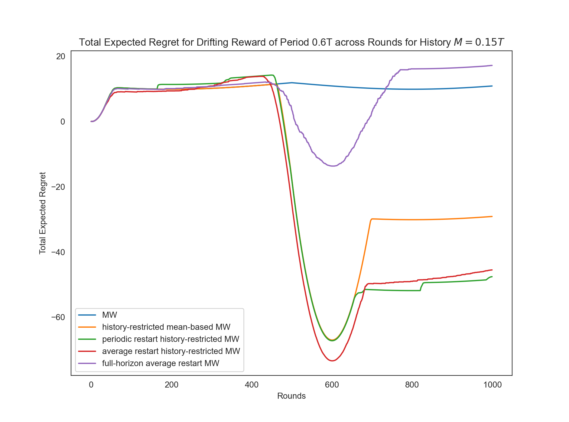
(h) $\varphi=3T/5$.

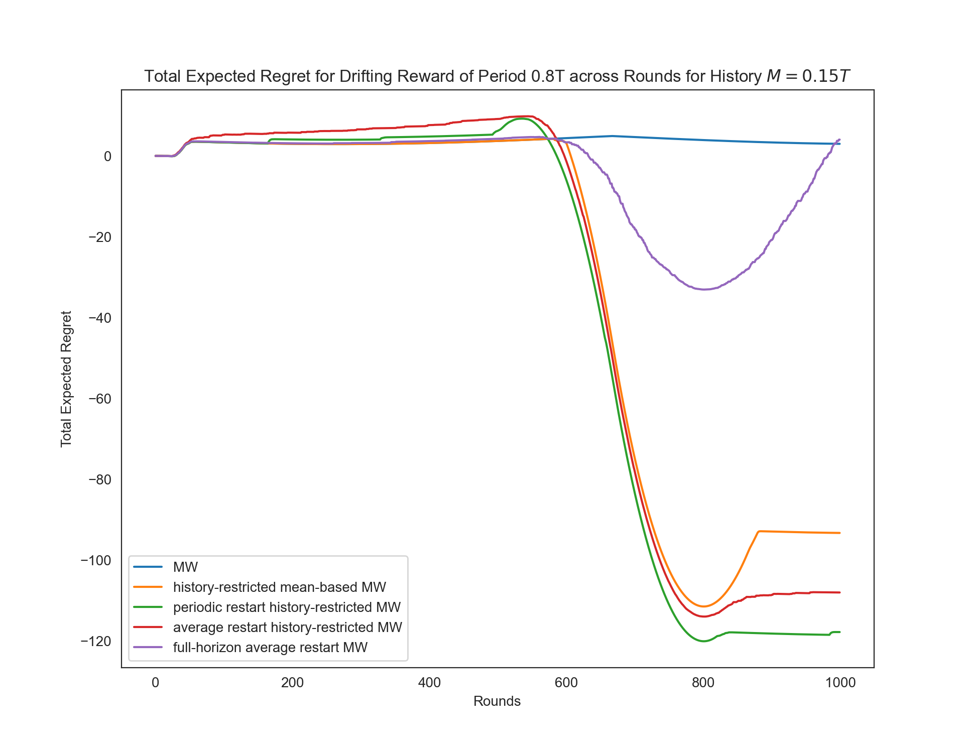
(i) $\varphi=4T/5$.

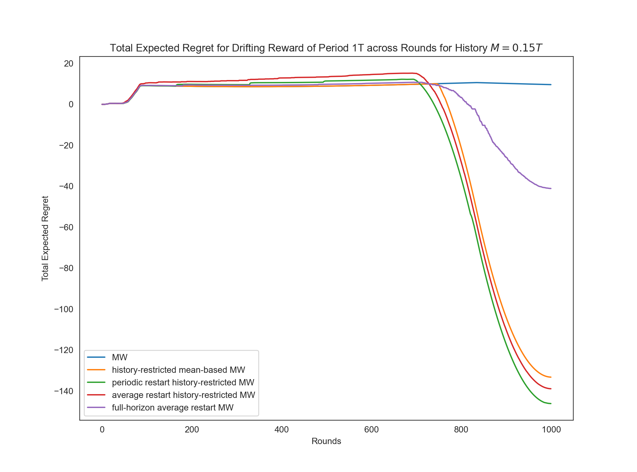
(j) $\varphi=T$.

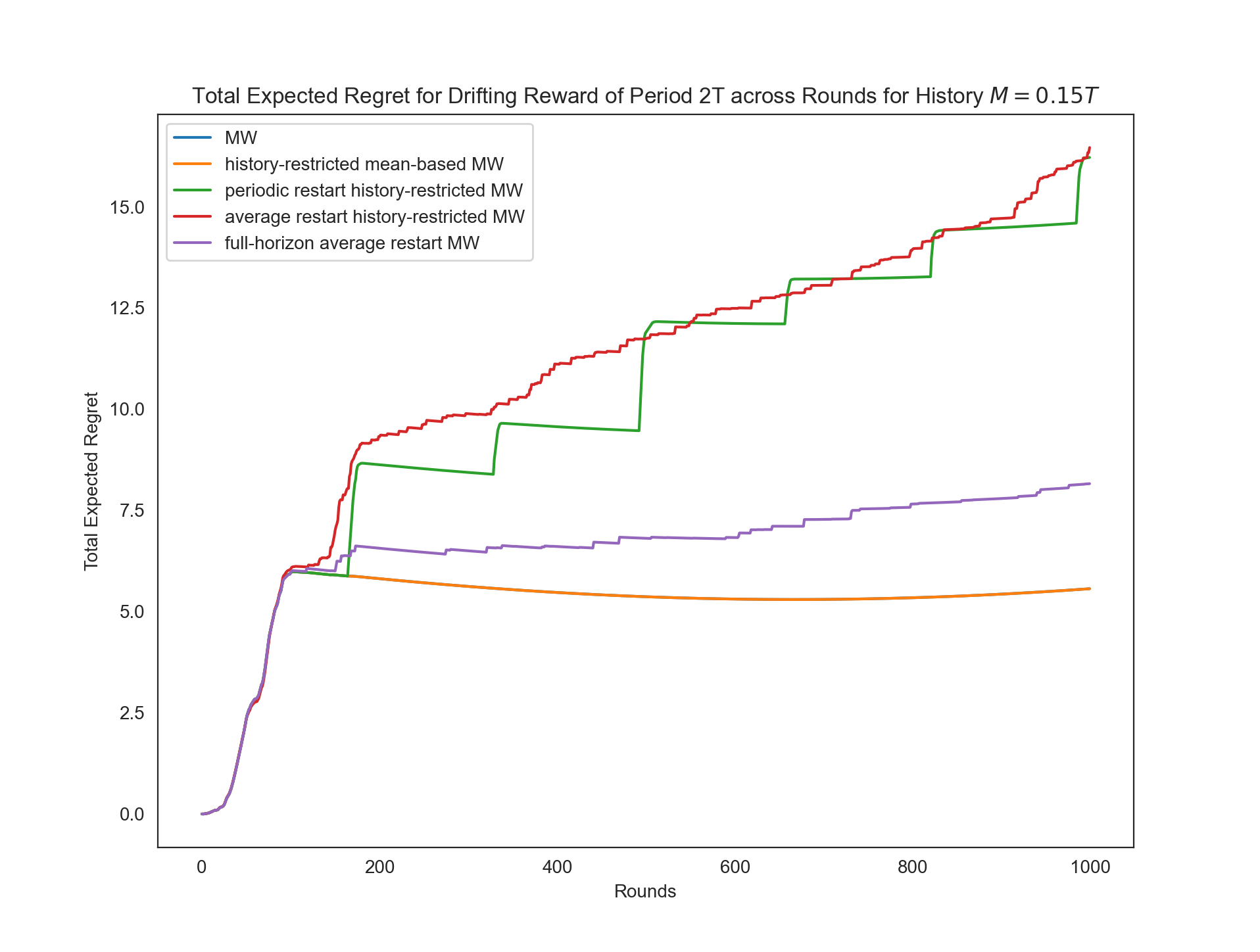
(k) $\varphi=2T$.

Figure 10: We plot the total regret of the algorithms over time for various drifting scenarios parameterized by periods $\varphi$.

Appendix D Ablations across the History Parameter

In this section, we study the average expected regret as a function of the history parameter $M$ in our history-restricted algorithms in multiple reward settings and across all algorithms.

Our takeaways are as follows:

1. There appear to qualitatively be two extreme modes of performance with respect to the choice of the history parameter in our various settings, which depends on the “periodicity” of the reward sequence: The first mode is “stochastic reward”-like – in this case, the history parameter does not affect performance greatly, except perhaps for very small choices of $M$, in which case the history-restricted algorithms typically perform worse than Multiplicative Weights (see the random walk rewards for small $\sigma$, as well as the periodic rewards for either very small or very large $\varphi$). The second mode is “periodic reward”-like – in this case, the history parameter has a significant impact on the performance of the history-restricted algorithms (and the full-horizon average restart algorithm) (see the random walk rewards for larger $\sigma$ as well as the periodic rewards for medium sized $\varphi$ and the paired periodic rewards where $\varphi_{1}$ and $\varphi_{2}$ are close together). In particular, the history-restricted algorithms significantly outperform Multiplicative Weights for smaller $M$, and gradually approach the performance of Multiplicative Weights for larger $M$, though some algorithms (typically the history-restricted and full-horizon average restart methods) level off with a strictly better performance than Multiplicative Weights.

2. Our periodic restart algorithm (Algorithm 1) performs well when $M$ is small, but in many settings, as $M$ gets larger, its performance takes a hit in comparison to the average restart method (Algorithm 2).

3. The full-horizon average restart method can significantly outperform Multiplicative Weights in settings where the reward is significantly periodic (including various periodic reward settings and random walk settings with larger standard deviation). This behavior is quite interesting since this algorithm is no-regret and demonstrates qualitatively different behavior compared to mean-based methods. Moreover, in the settings we considered, the full-horizon average restart method is never worse than Multiplicative Weights. It would be interesting to compare this algorithm to other methods from the adaptive online learning literature, though we suspect that those methods (e.g., (Erven et al., 2011; Chastain et al., 2013; Koolen et al., 2016; Mourtada and Gaïffas, 2019)) tend to be more focused on bridging the gap between the good performance of Follow-the-Leader (FTL) in stochastic settings and Multiplicative Weights in adversarial settings to get the best of both worlds – In our experiments, we noted that the FTL algorithm performed essentially identically to MW in our settings, and thus the adaptive gains possible in our periodic and drifting rewards settings are not necessarily exploitable by prior methods.

4. We observe that the history-restricted average restart method typically outperforms the full-horizon average restart algorithm especially for smaller values of $M$ in “periodic-reward-like” settings, and it gets worse as $M$ increases roughly monotonically until it approaches the performance of the full-horizon average restart method.

For ease of reading the plots, we also include a map between the algorithm and the color of its performance graphs in the plots below:

1. Multiplicative Weights (MW): Blue

2. History-Restricted Periodic Restart (Algorithm 1): Green

3. History-Restricted Average Restart (Algorithm 2): Red

4. Full-Horizon Average Restart (Algorithm  3): Purple

5. History-Restricted Mean-Based (Algorithm 4): Orange

D.1 Average Regret vs. History

D.1.1 Random Walk Rewards

Note for the random walk settings that there are essentially two plots against history which show up for the settings we consider: a) a plot similar to the stochastic setting (this plot occurs when the random walk behavior oscillates around an even coin flip, and is thus very similar to the stochastic setting); b) a plot similar to some of the periodic settings – this happens when significant non-stationarity arises over the course of the random walk – this is more likely to happen for larger values of $\sigma$.

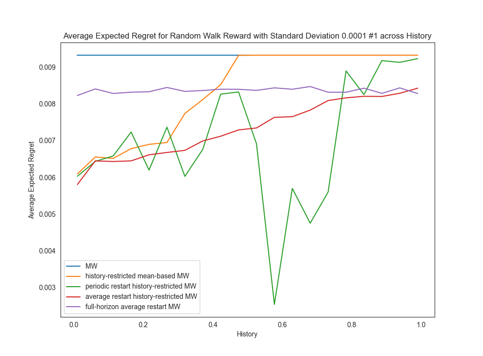
(a) Random Walk $\#1$

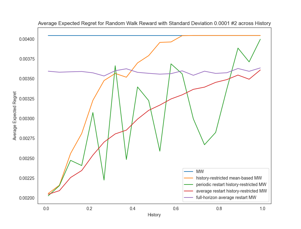
(b) Random Walk $\#2$

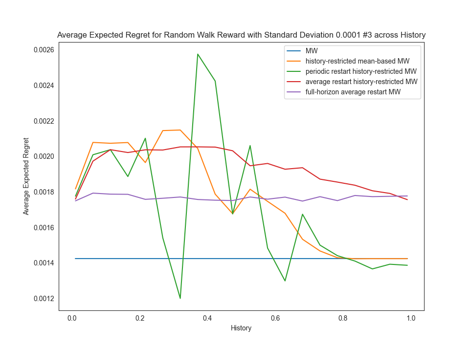
(c) Random Walk $\#3$

Figure 11: We compare the average regret of our different algorithms across different choices of history for a random walk setting where $\sigma=0.0001$.

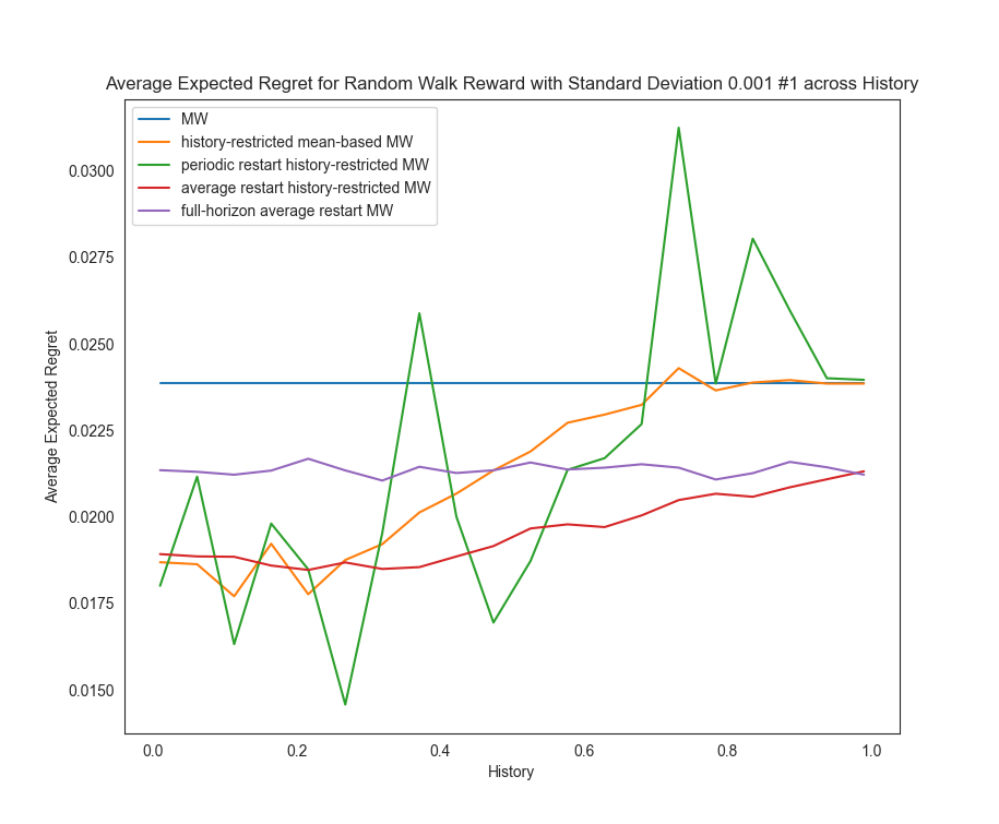
(a) Random Walk $\#1$

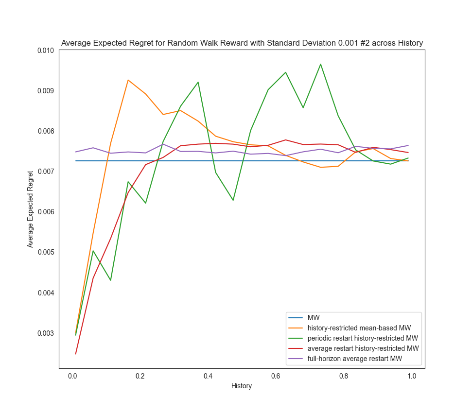
(b) Random Walk $\#2$

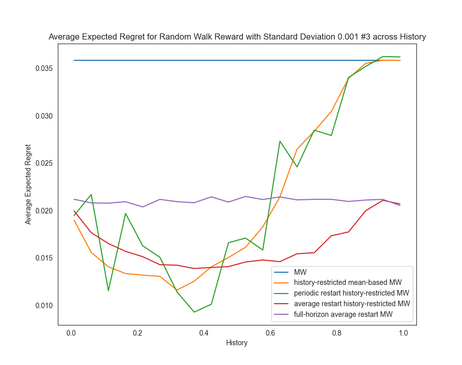
(c) Random Walk $\#3$

Figure 12: We compare the average regret of our different algorithms across different choices of history for a random walk setting where $\sigma=0.001$.

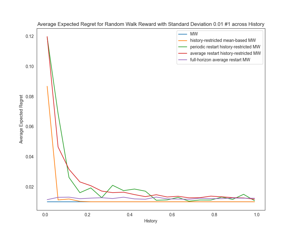
(a) Random Walk $\#1$

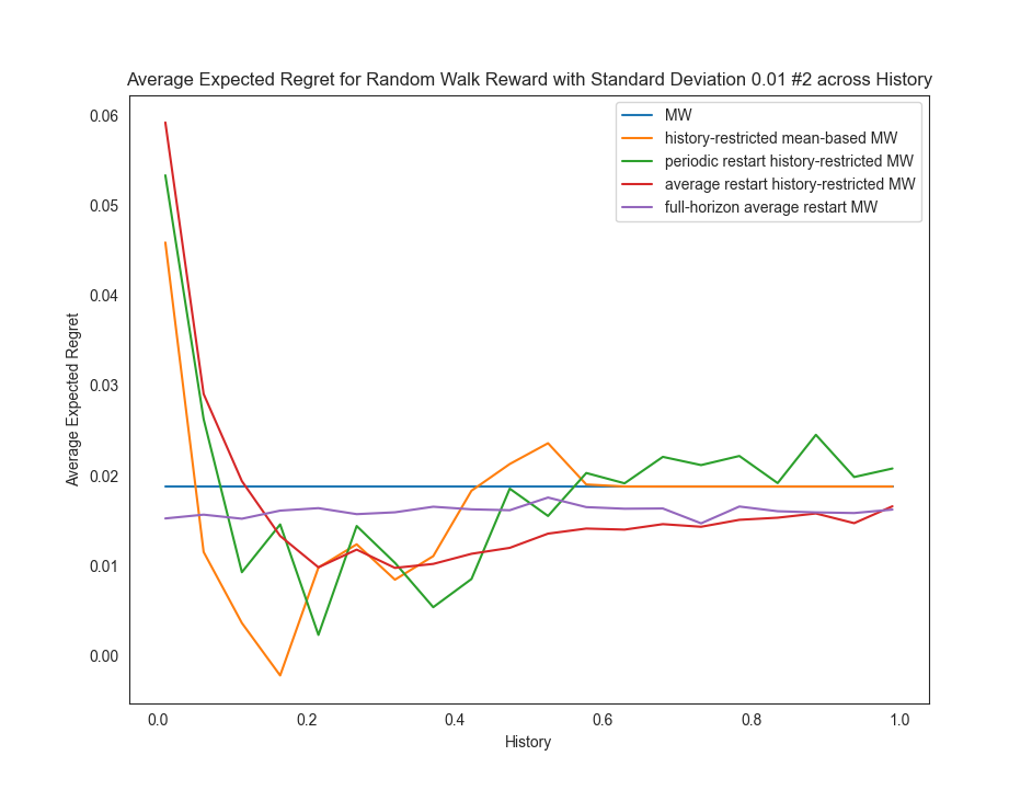
(b) Random Walk $\#2$

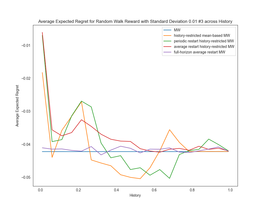
(c) Random Walk $\#3$

Figure 13: We compare the average regret of our different algorithms across different choices of history for a random walk setting where $\sigma=0.01$.

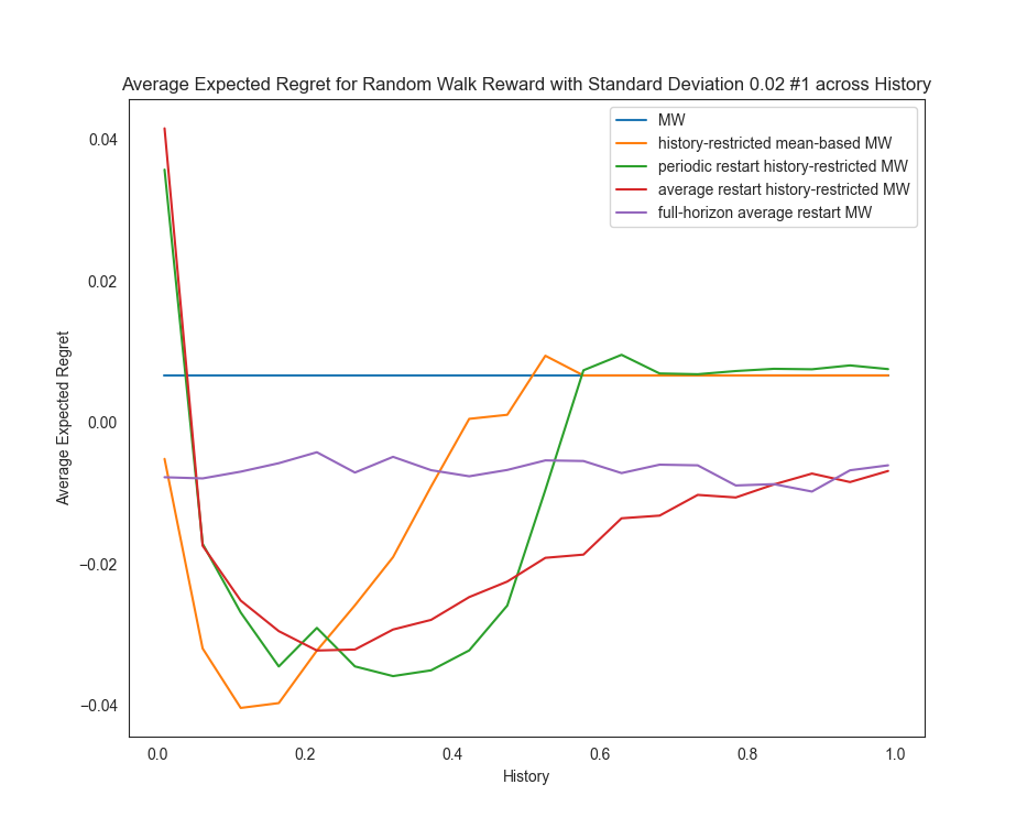
(a) Random Walk $\#1$

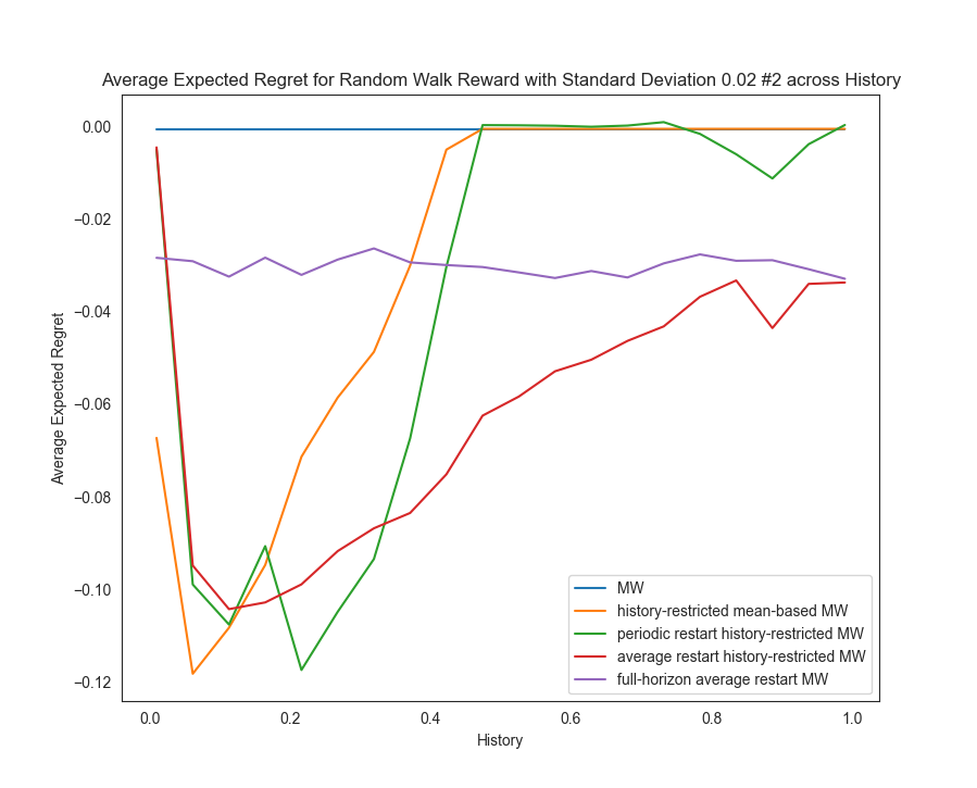
(b) Random Walk $\#2$

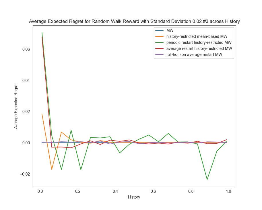
(c) Random Walk $\#3$

Figure 14: We compare the average regret of our different algorithms across different choices of history for a random walk setting where $\sigma=0.02$.

D.1.2 Periodic Rewards

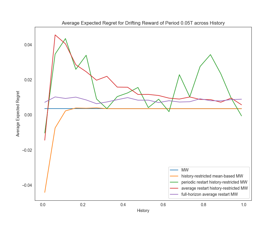
(a) $\varphi=T/20$

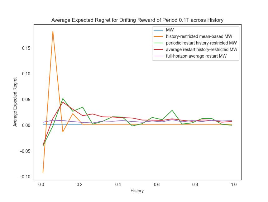
(b) $\varphi=T/10$

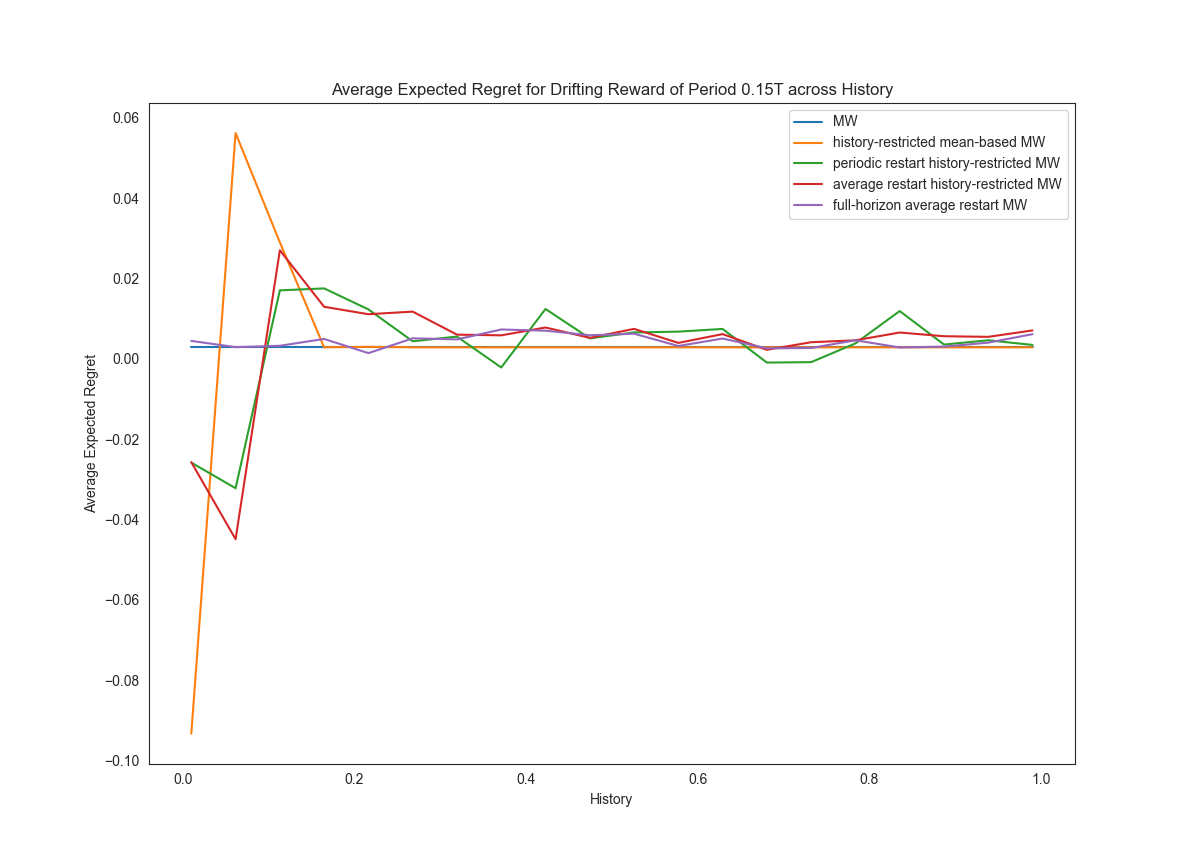
(c) $\varphi=0.15T$

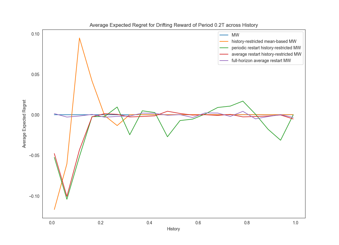
(d) $\varphi=T/5$

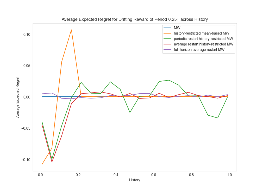
(e) $\varphi=T/4$

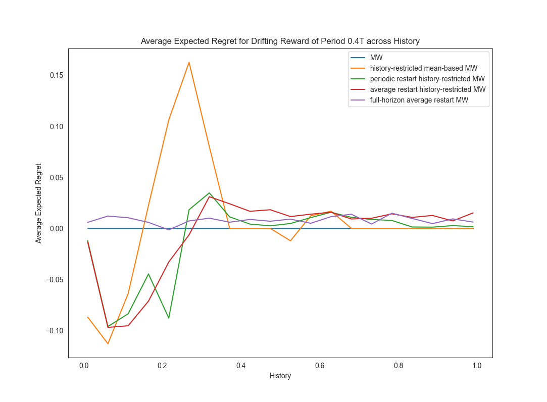
(f) $\varphi=2T/5$

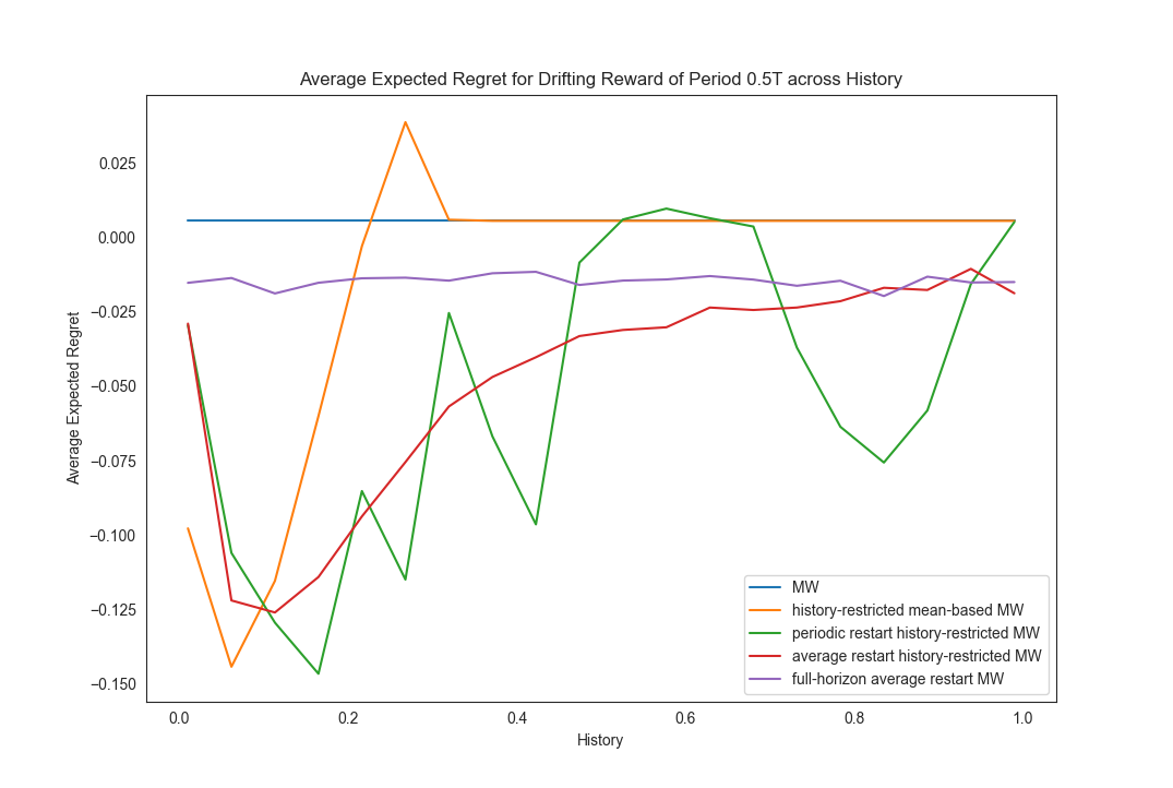
(g) $\varphi=T/2$

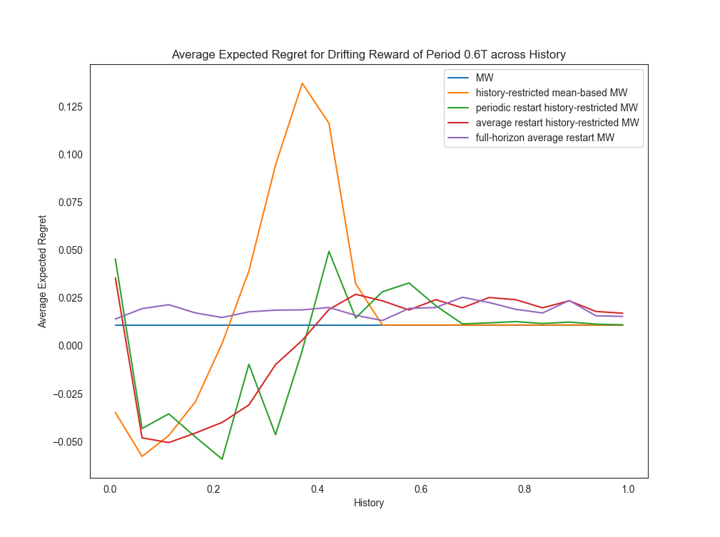
(h) $\varphi=3T/5$

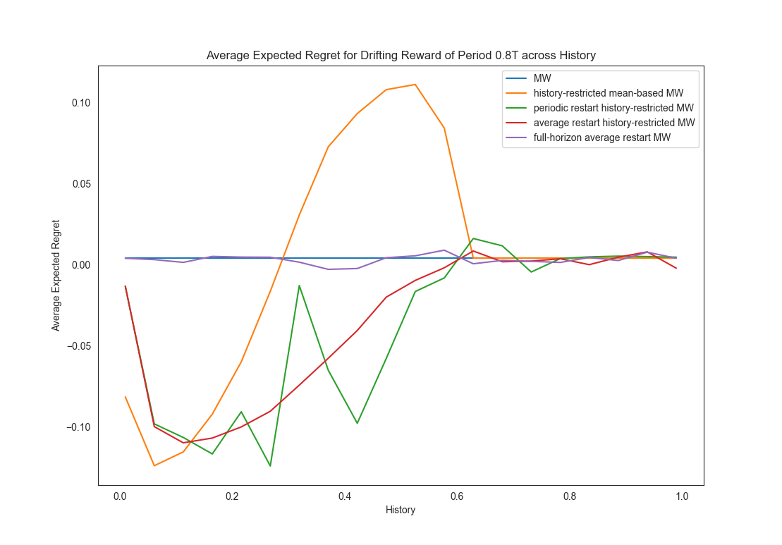
(i) $\varphi=4T/5$

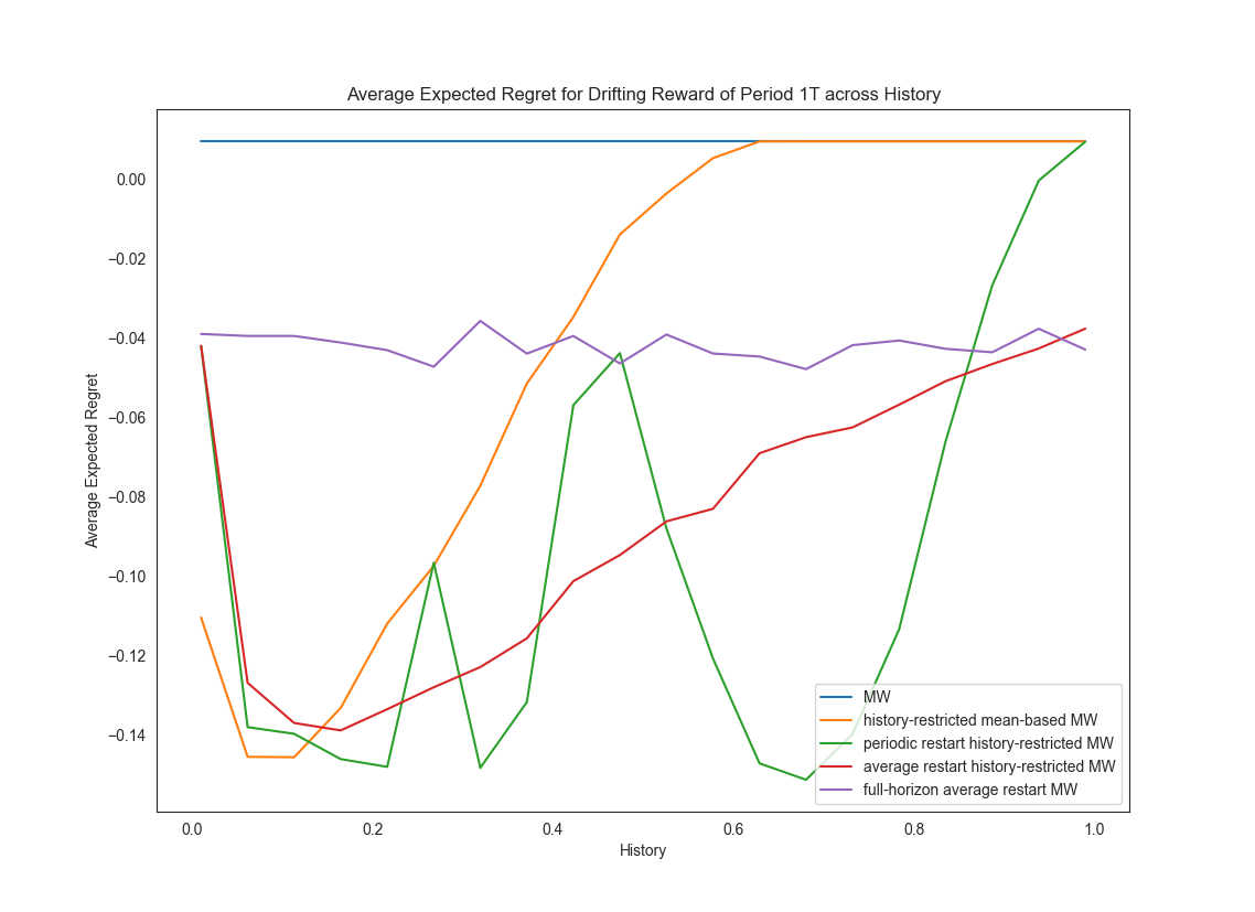
(j) $\varphi=T$

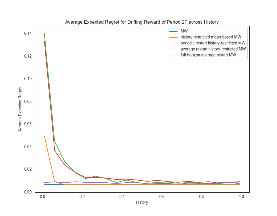
(k) $\varphi=2T$

Figure 15: We compare the average regret of our different algorithms across different choices of history for various drifting settings, parameterized by period $\varphi$.

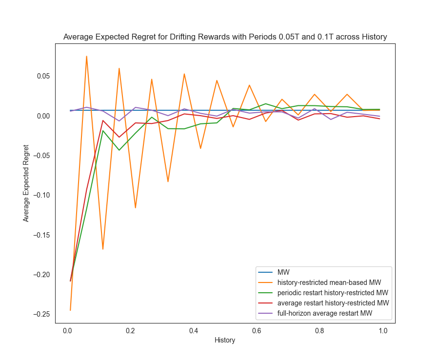
(a) $\varphi_{2}=T/10$

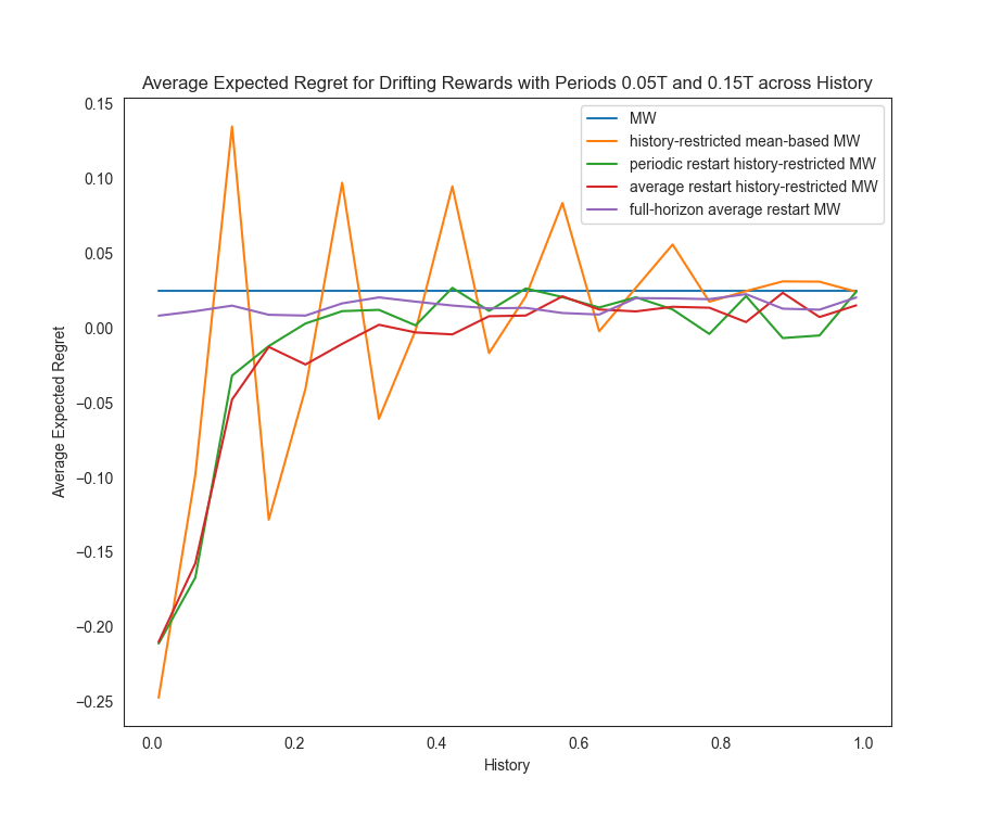
(b) $\varphi_{2}=0.15T$

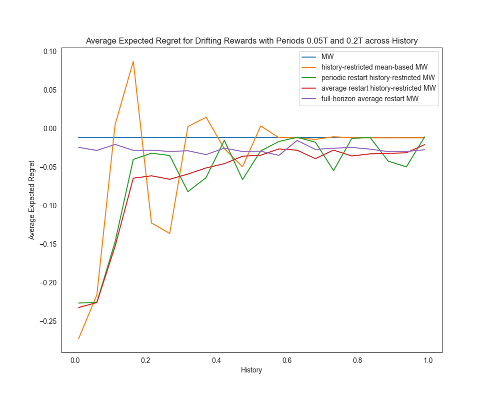
(c) $\varphi_{2}=T/5$

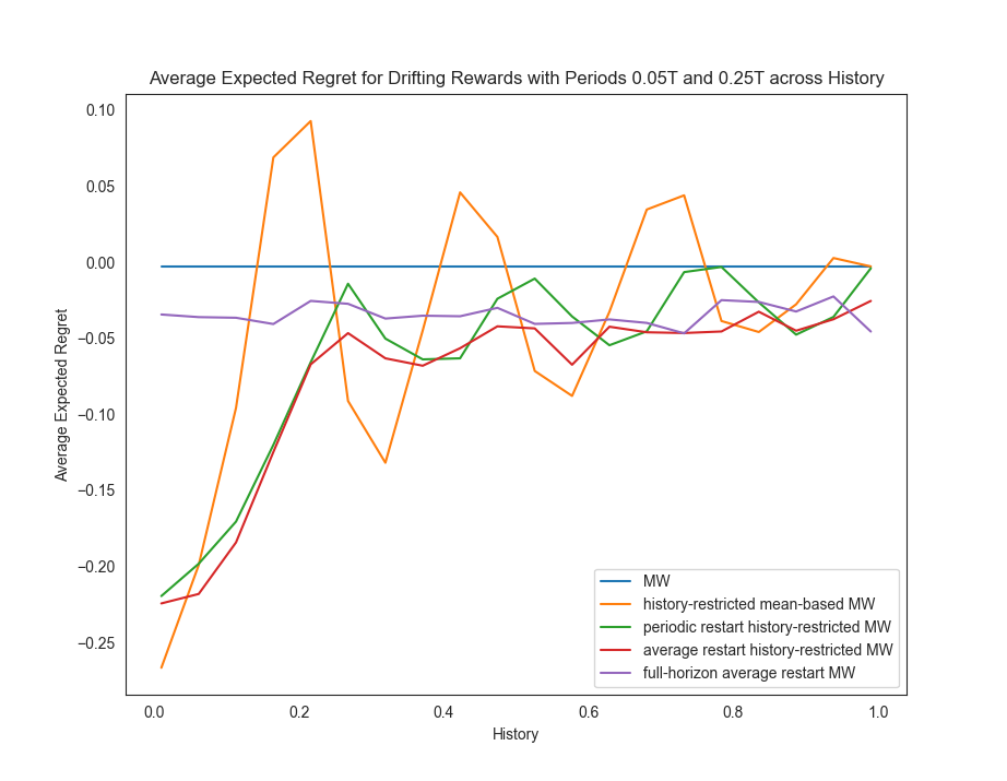
(d) $\varphi_{2}=T/4$

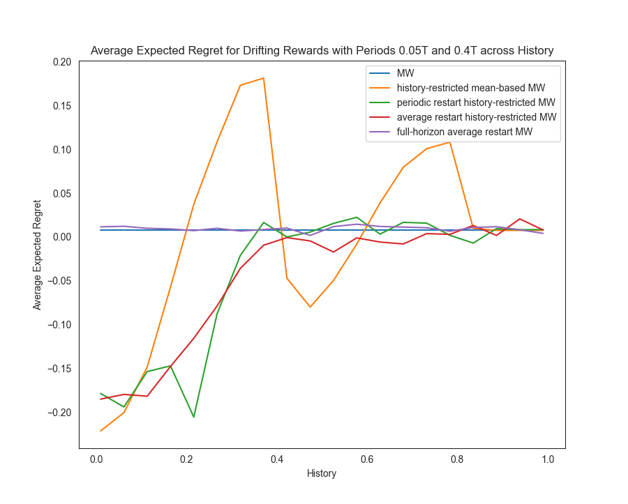
(e) $\varphi_{2}=2T/5$

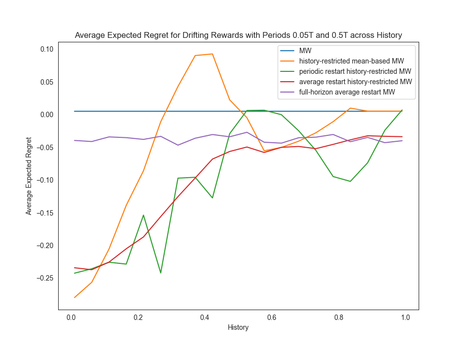
(f) $\varphi_{2}=T/2$

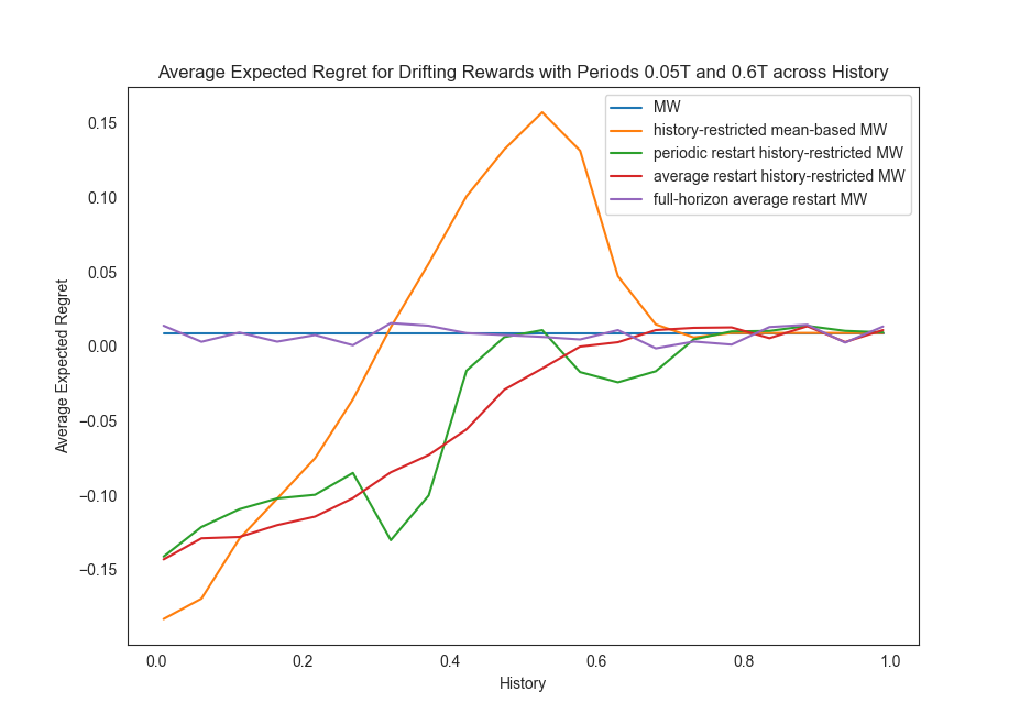
(g) $\varphi_{2}=3T/5$

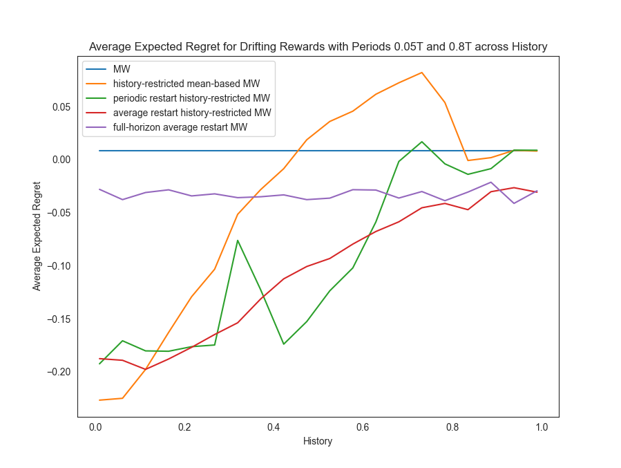
(h) $\varphi_{2}=4T/5$

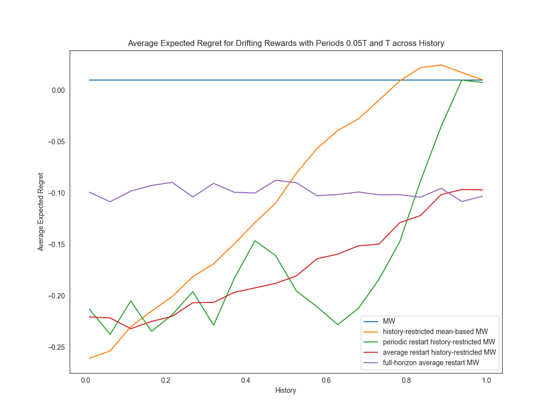
(i) $\varphi_{2}=T$

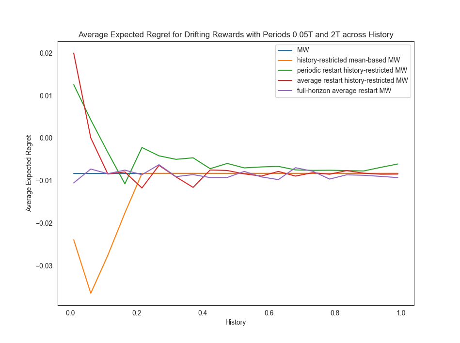
(j) $\varphi_{2}=2T$

Figure 16: We compare the average regret of our different algorithms across different choices of history for various drifting settings, with first arm having period $\varphi_{1}=T/20$ and second arm with period $\varphi_{2}$.

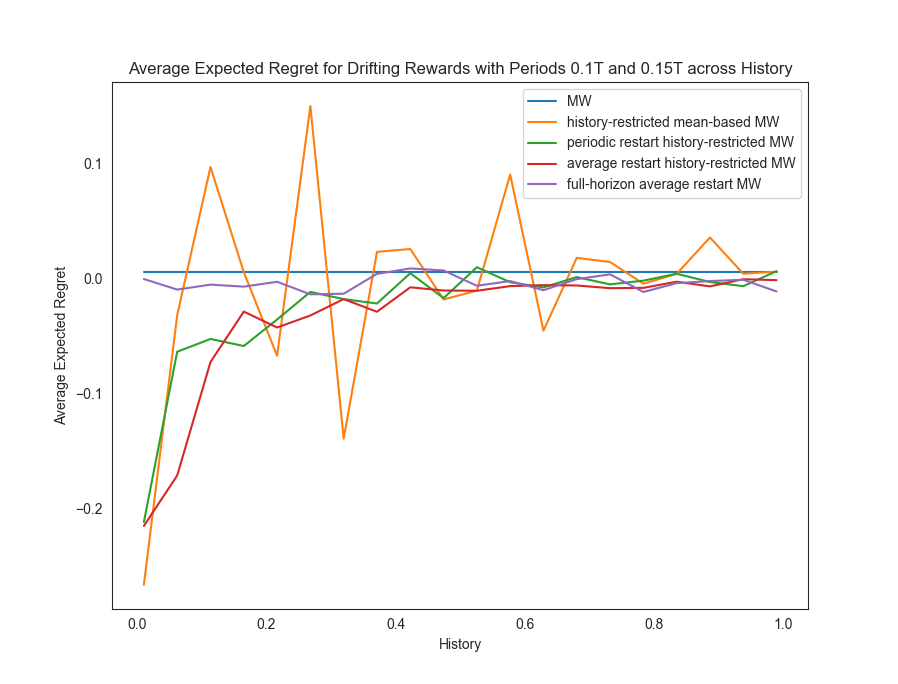
(a) $\varphi_{2}=0.15T$

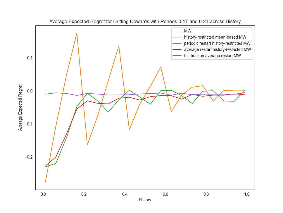
(b) $\varphi_{2}=T/5$

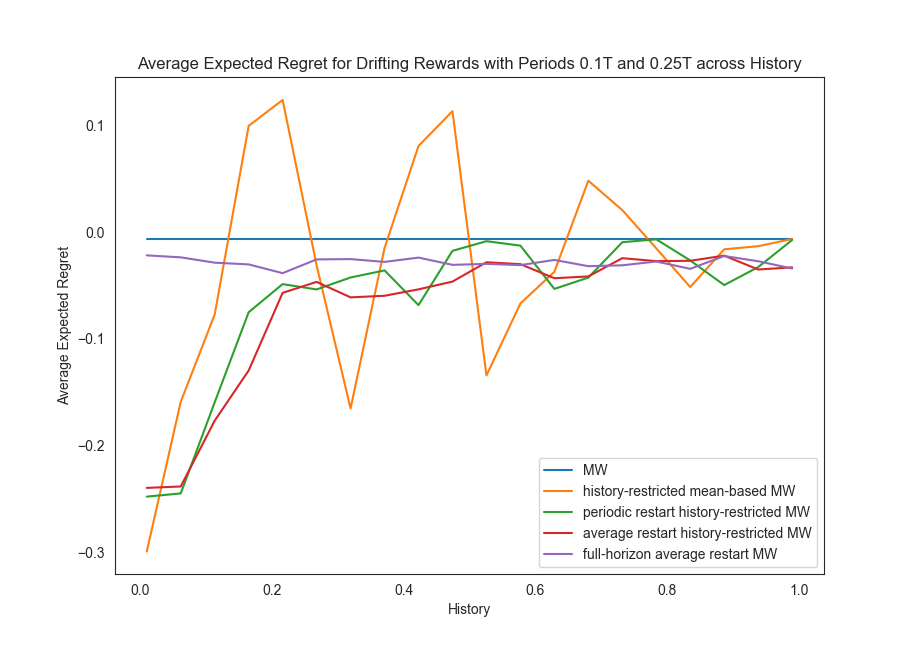
(c) $\varphi_{2}=T/4$

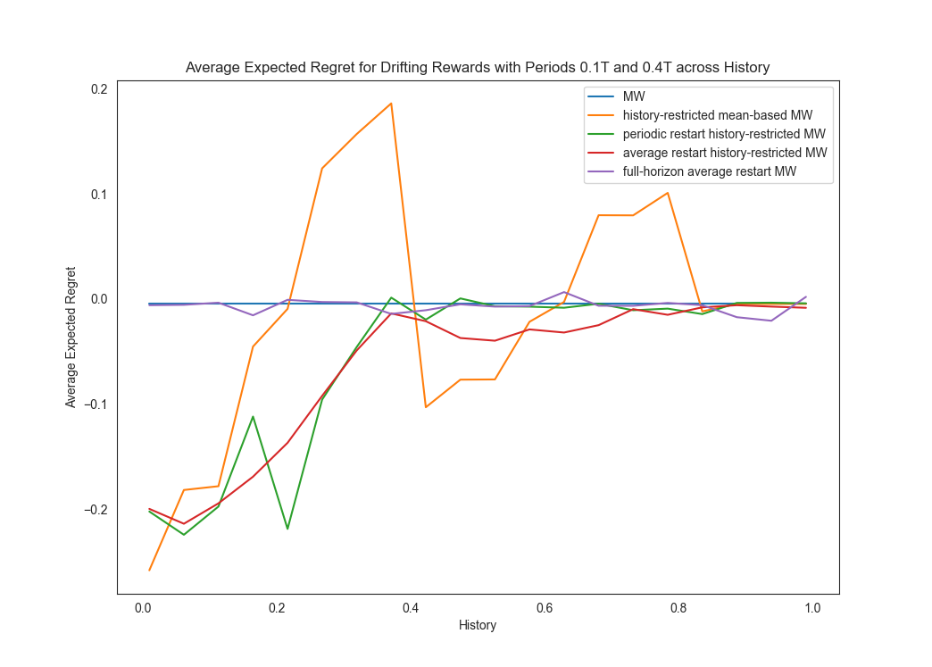
(d) $\varphi_{2}=2T/5$

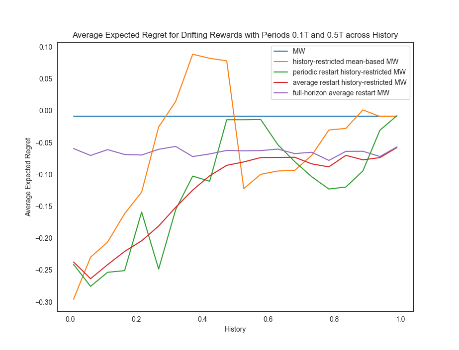
(e) $\varphi_{2}=T/2$

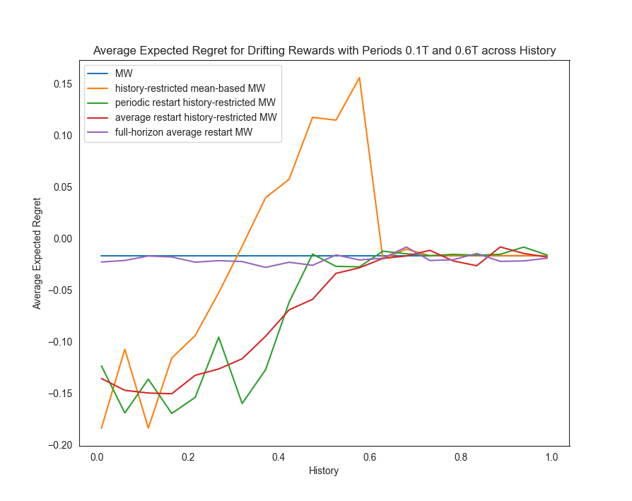
(f) $\varphi_{2}=3T/5$

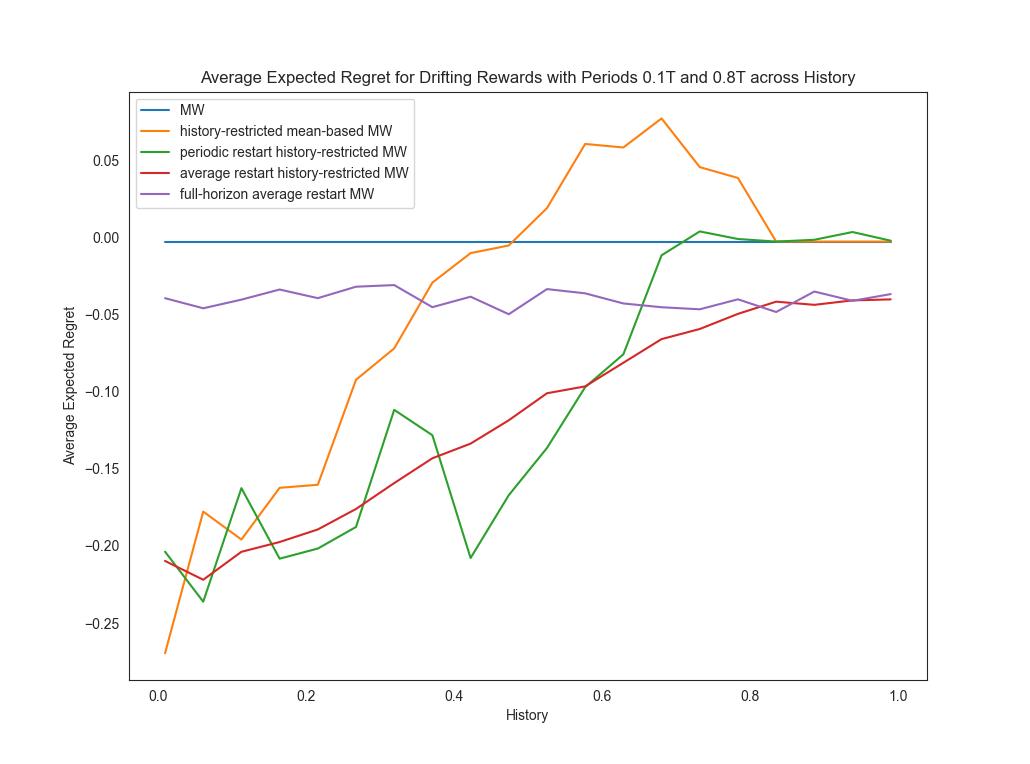
(g) $\varphi_{2}=4T/5$

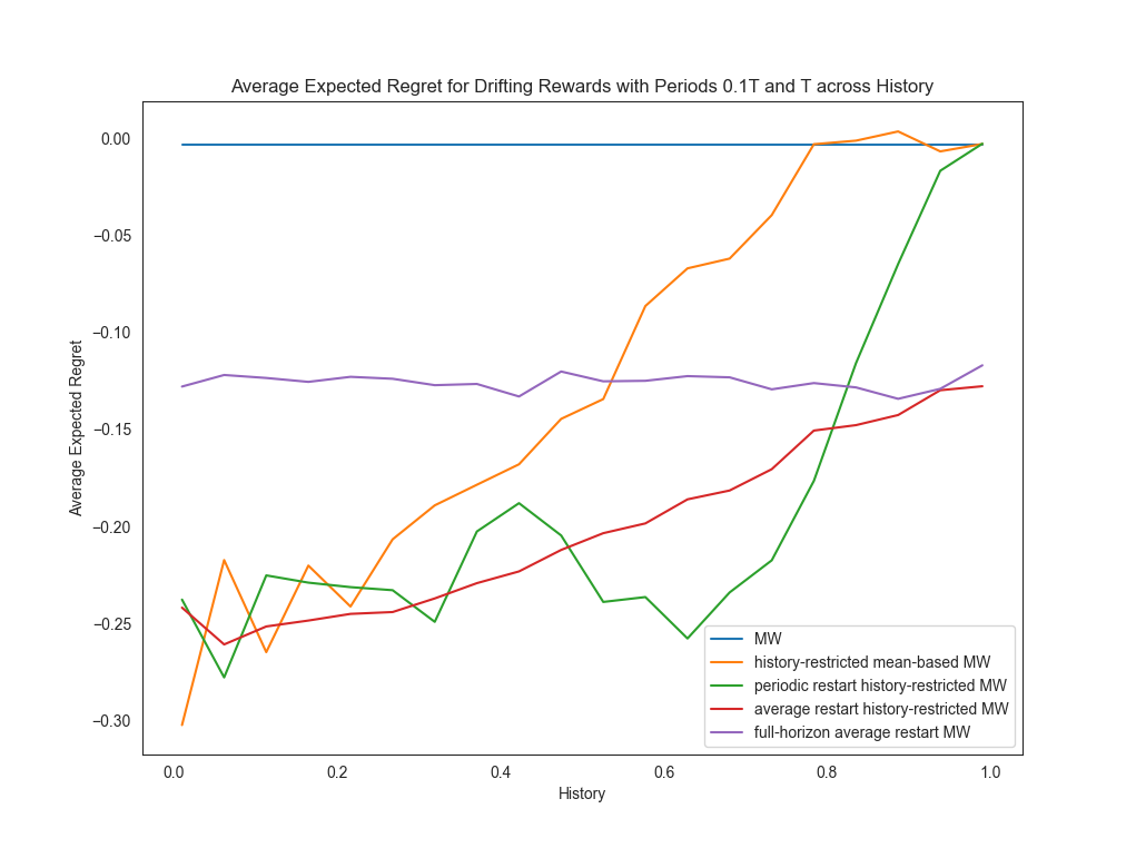
(h) $\varphi_{2}=T$

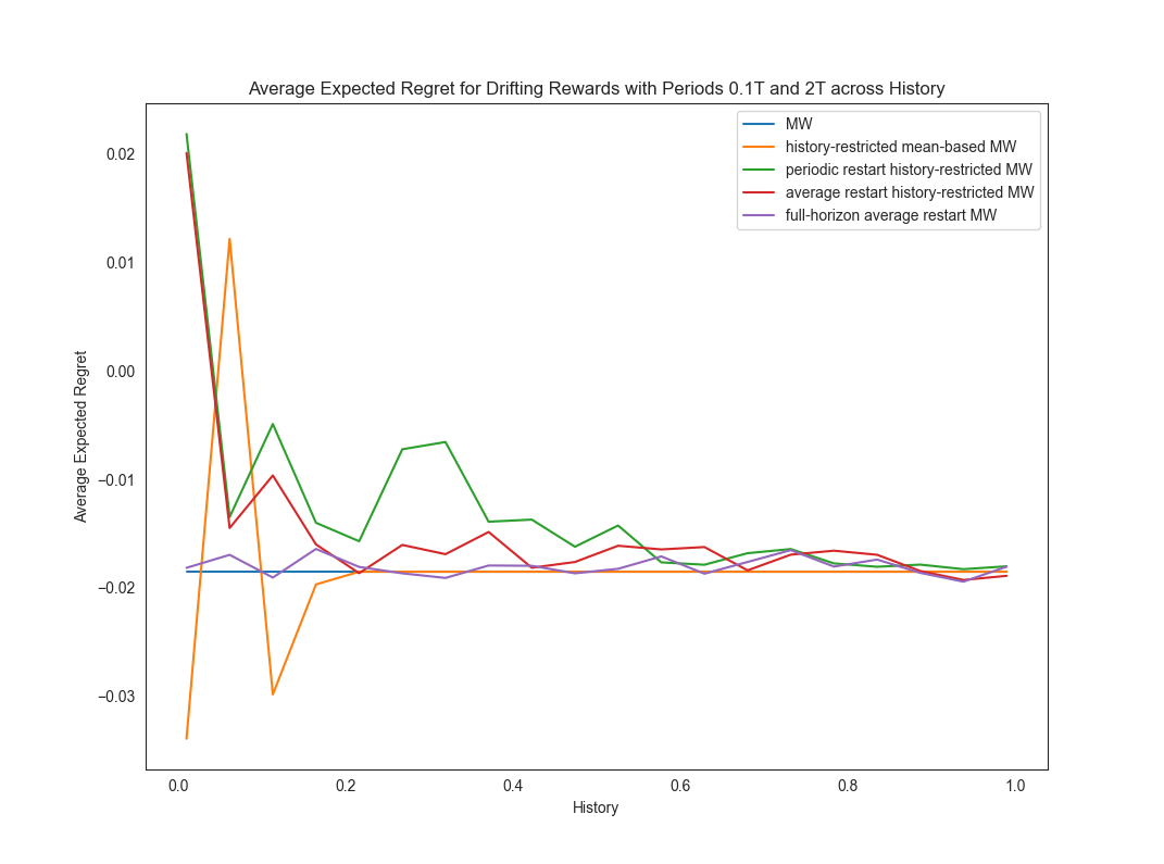
(i) $\varphi_{2}=2T$

Figure 17: We compare the average regret of our different algorithms across different choices of history for various drifting settings, with first arm having period $\varphi_{1}=T/10$ and second arm with period $\varphi_{2}$.

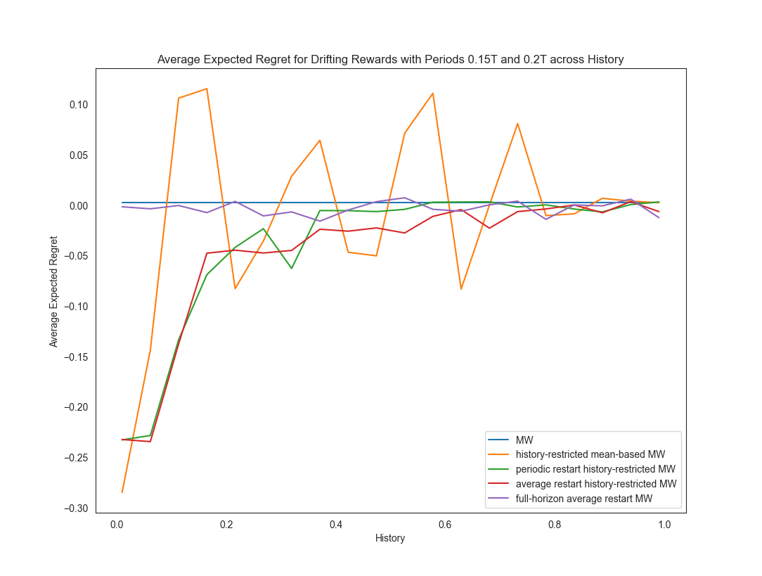
(a) $\varphi_{2}=T/5$

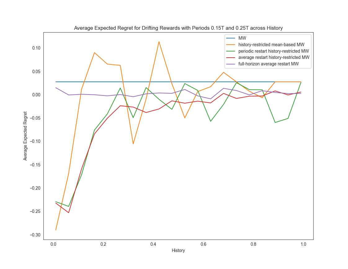
(b) $\varphi_{2}=T/4$

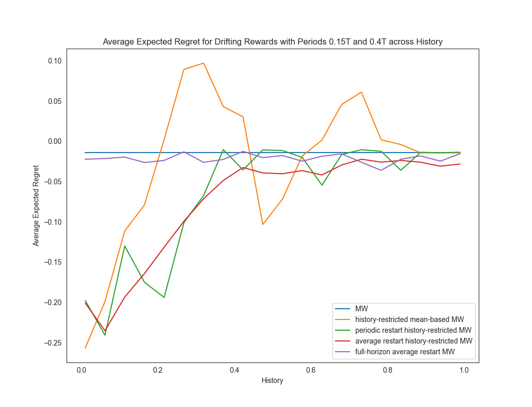
(c) $\varphi_{2}=2T/5$

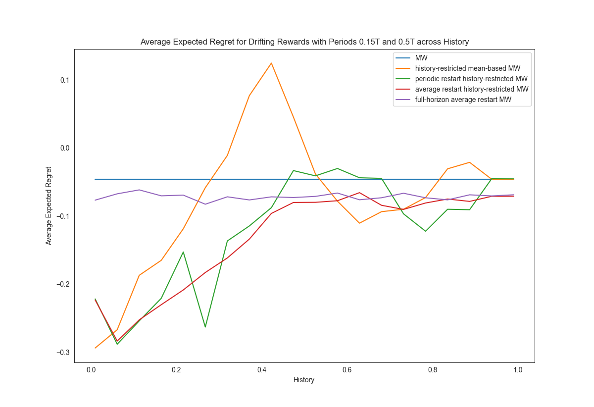
(d) $\varphi_{2}=T/2$

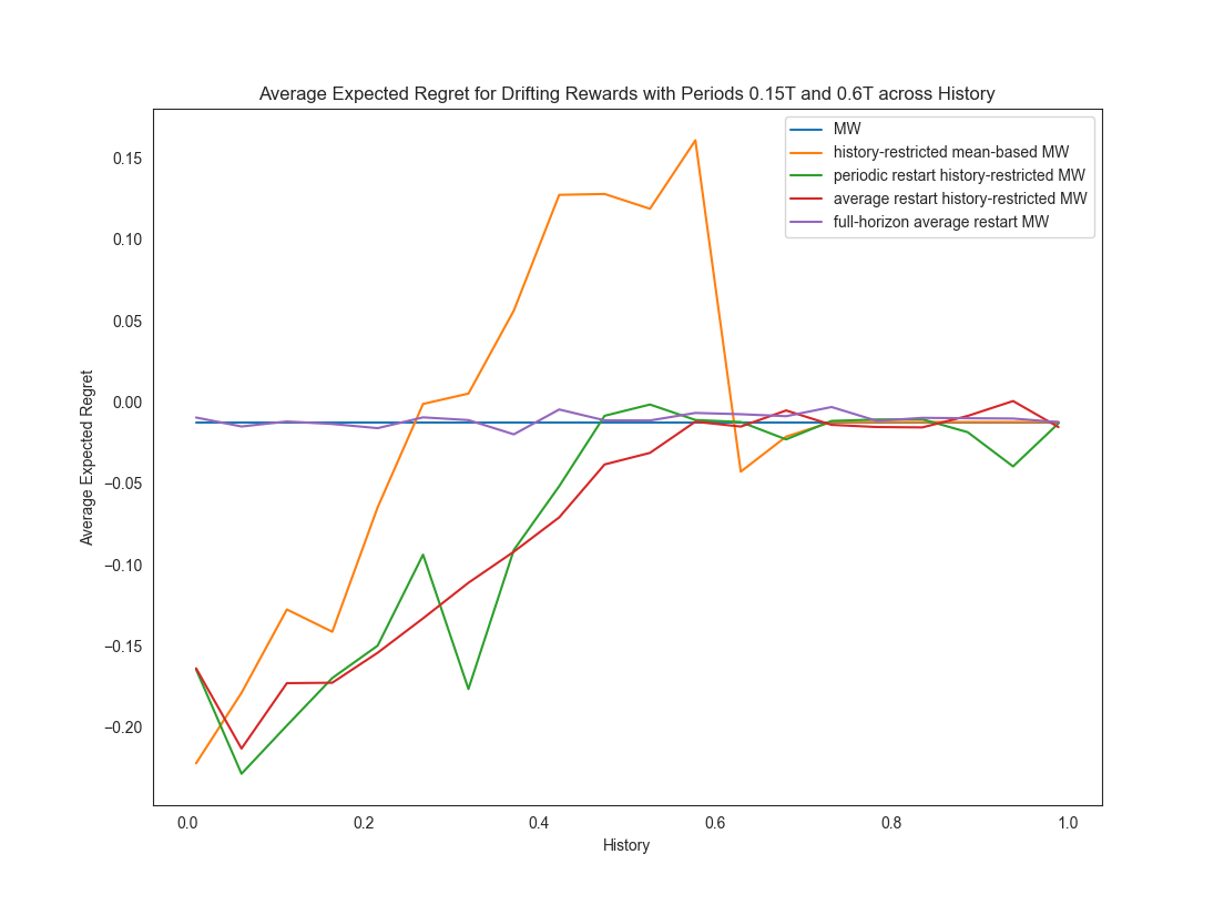
(e) $\varphi_{2}=3T/5$

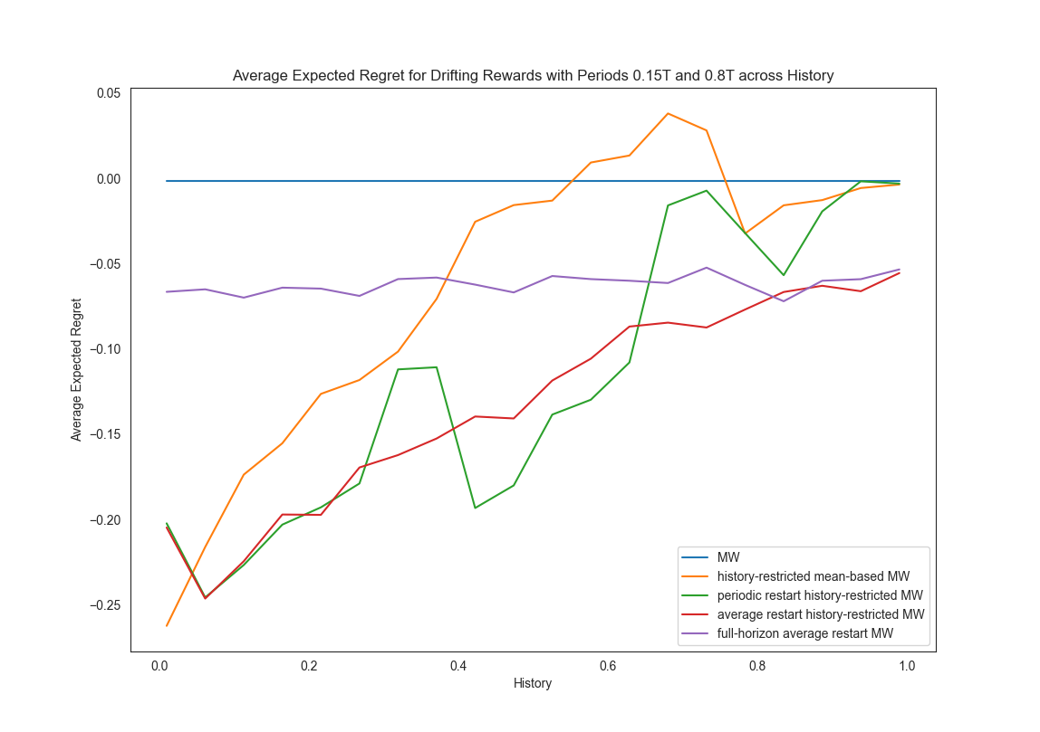
(f) $\varphi_{2}=4T/5$

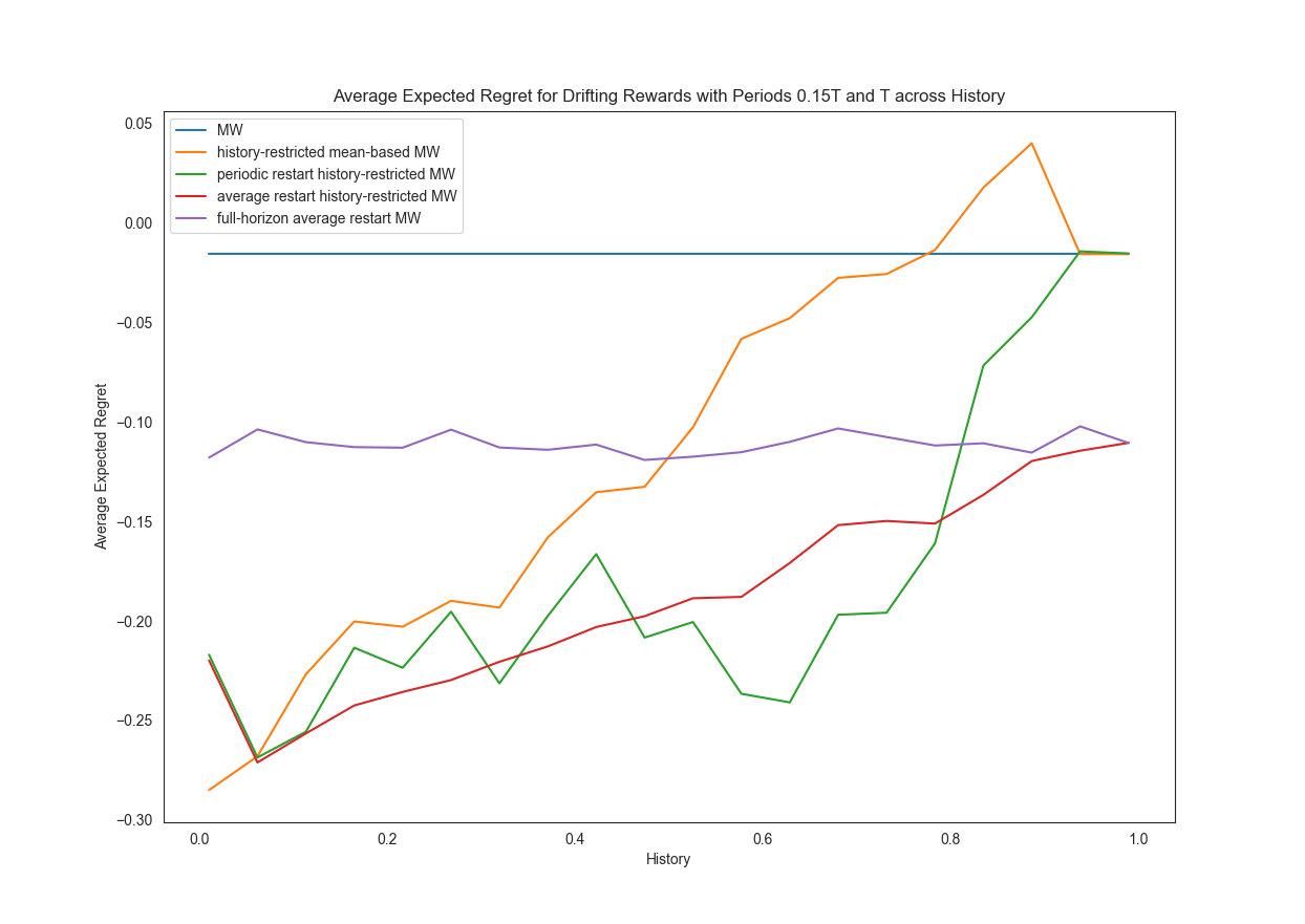
(g) $\varphi_{2}=T$

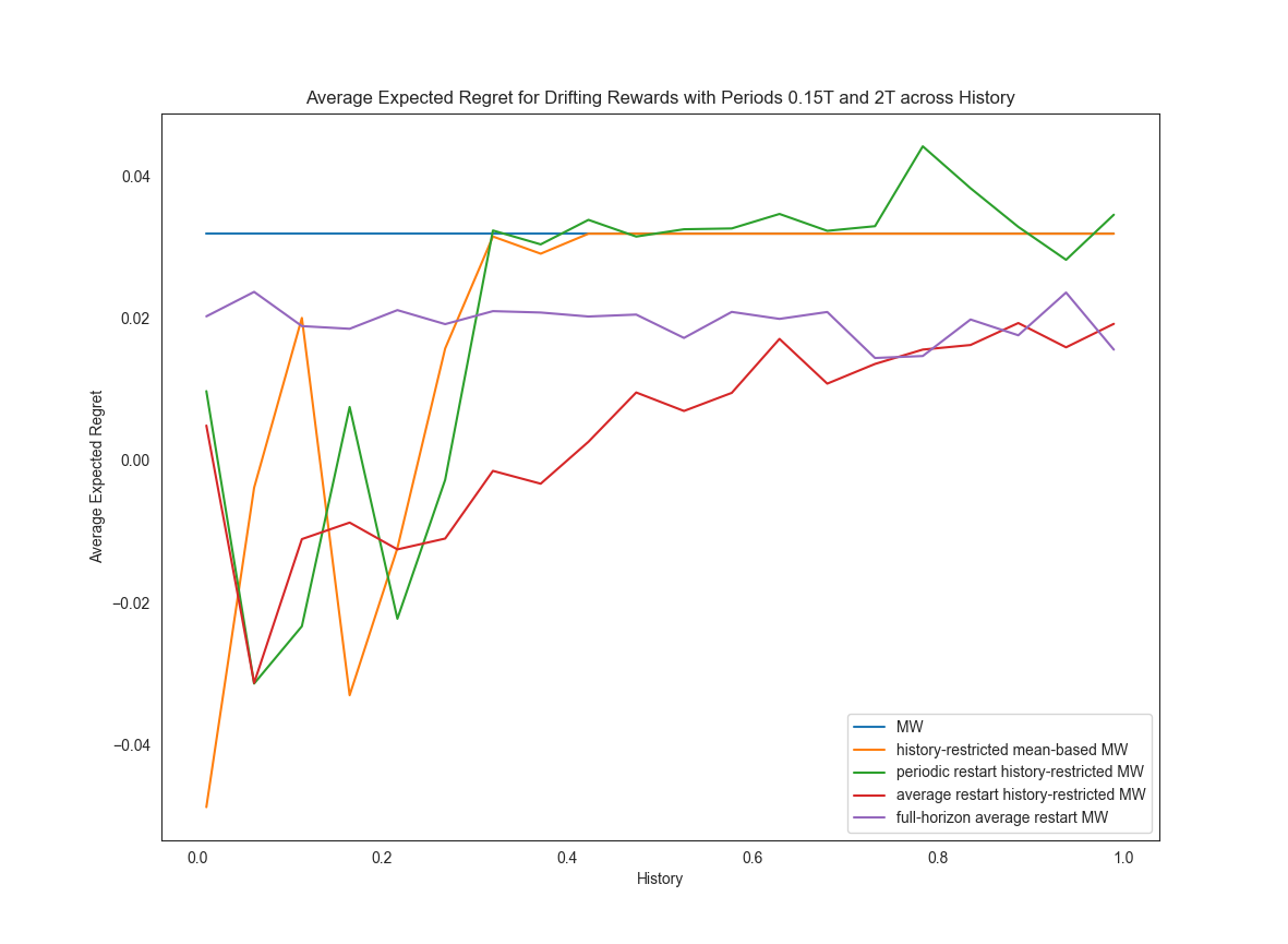
(h) $\varphi_{2}=2T$

Figure 18: We compare the average regret of our different algorithms across different choices of history for various drifting settings, with first arm having period $\varphi_{1}=0.15T$ and second arm with period $\varphi_{2}$.

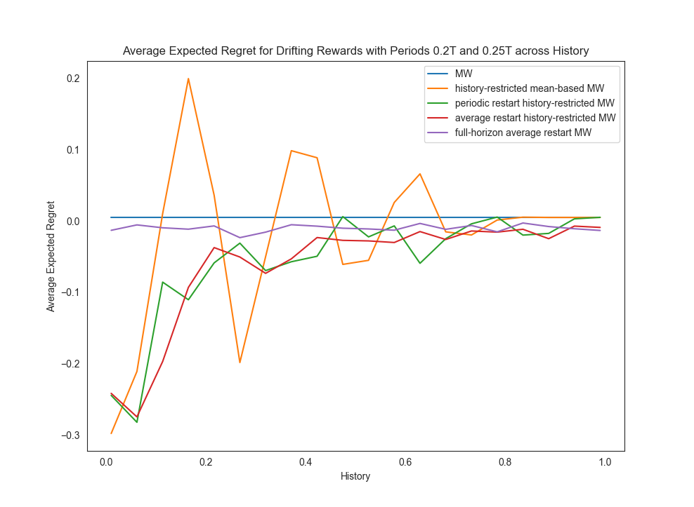
(a) $\varphi_{2}=T/4$

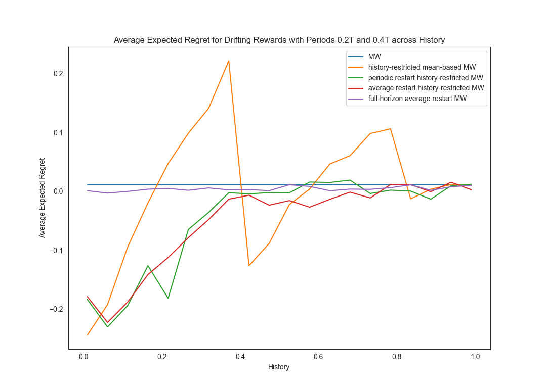
(b) $\varphi_{2}=2T/5$

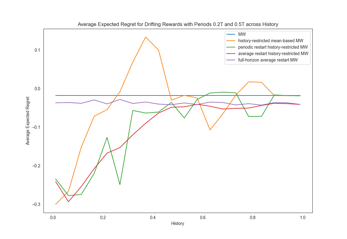
(c) $\varphi_{2}=T/2$

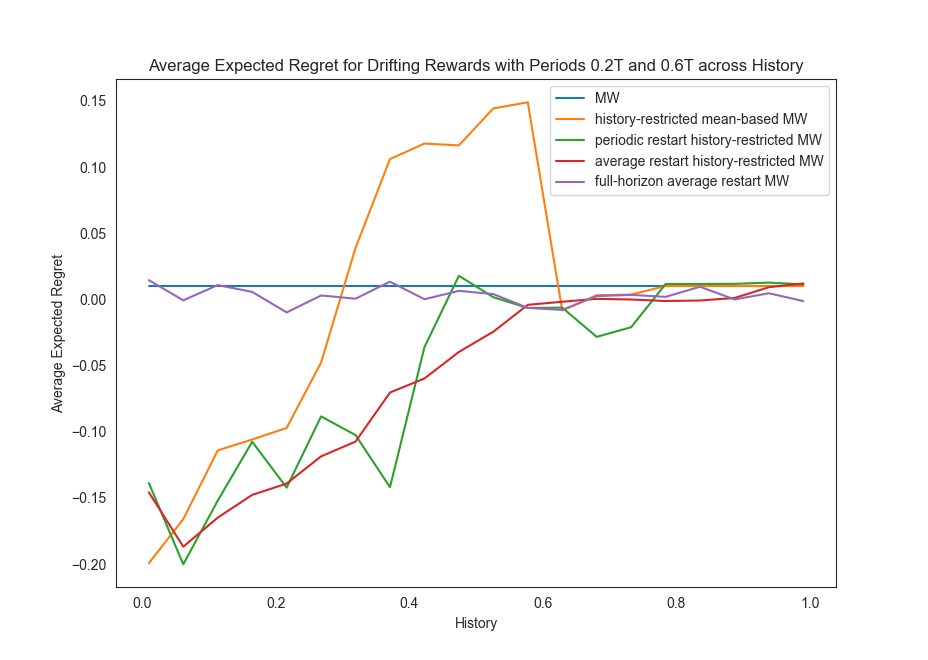
(d) $\varphi_{2}=3T/5$

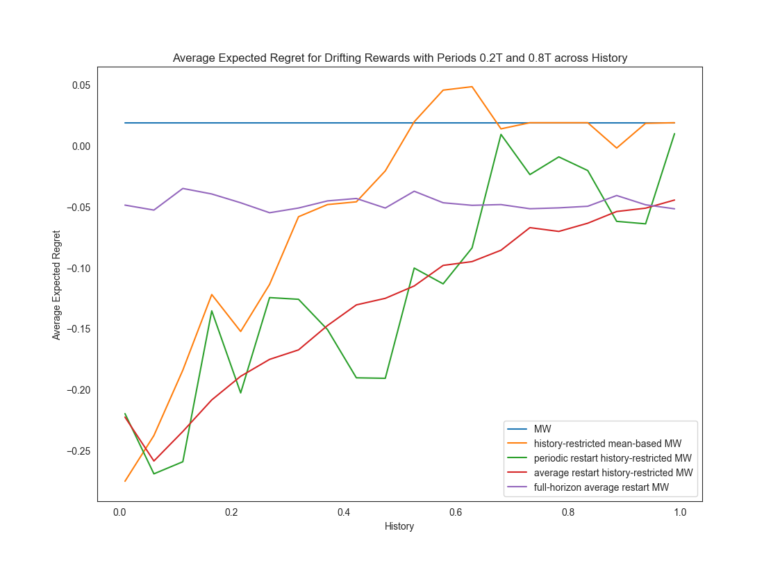
(e) $\varphi_{2}=4T/5$

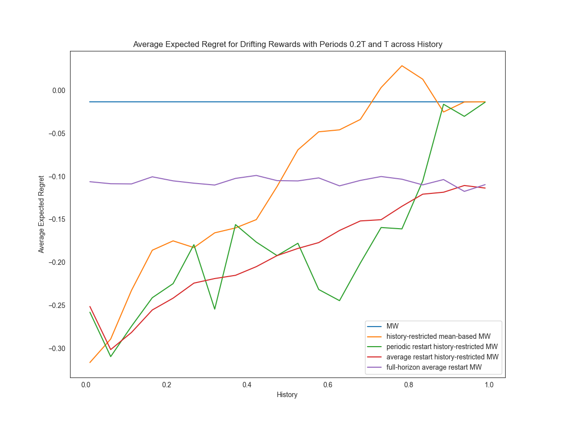
(f) $\varphi_{2}=T$

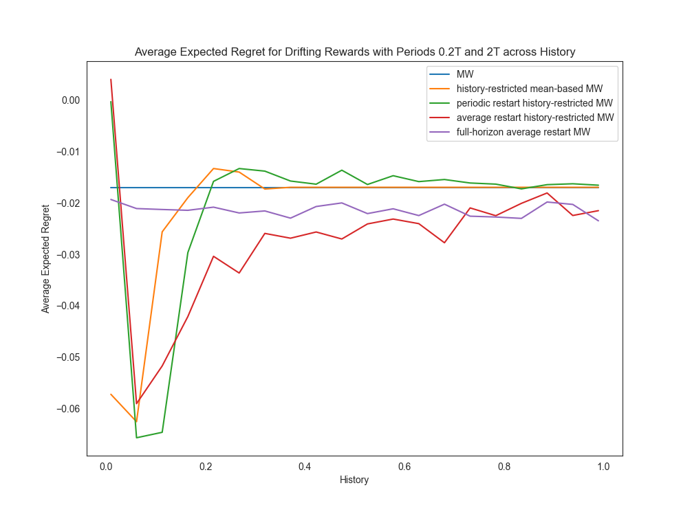
(g) $\varphi_{2}=2T$

Figure 19: We compare the average regret of our different algorithms across different choices of history for various drifting settings, with first arm having period $\varphi_{1}=T/5$ and second arm with period $\varphi_{2}$.

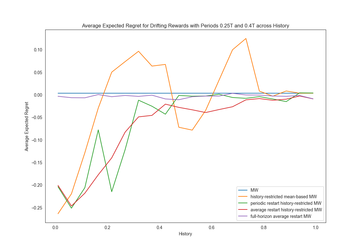
(a) $\varphi_{2}=2T/5$

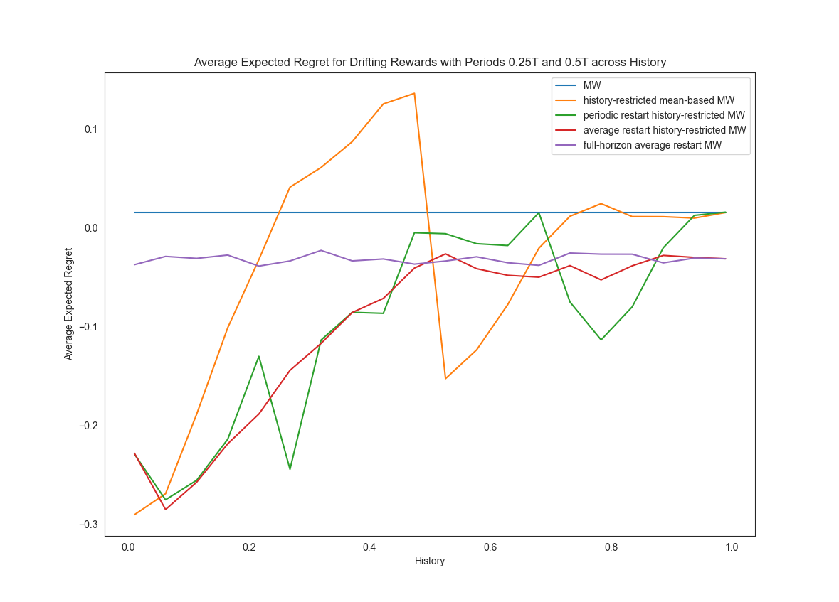
(b) $\varphi_{2}=T/2$

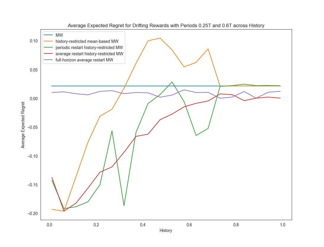
(c) $\varphi_{2}=3T/5$

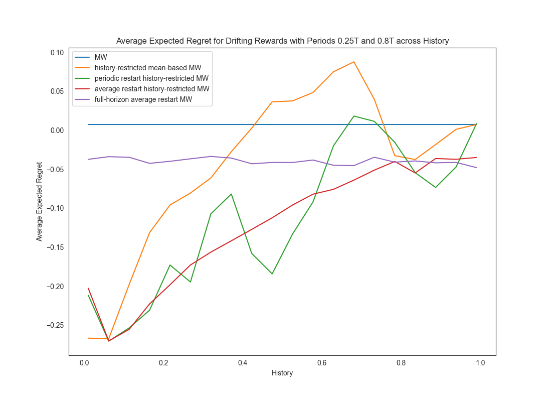
(d) $\varphi_{2}=4T/5$

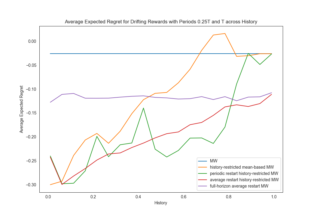
(e) $\varphi_{2}=T$

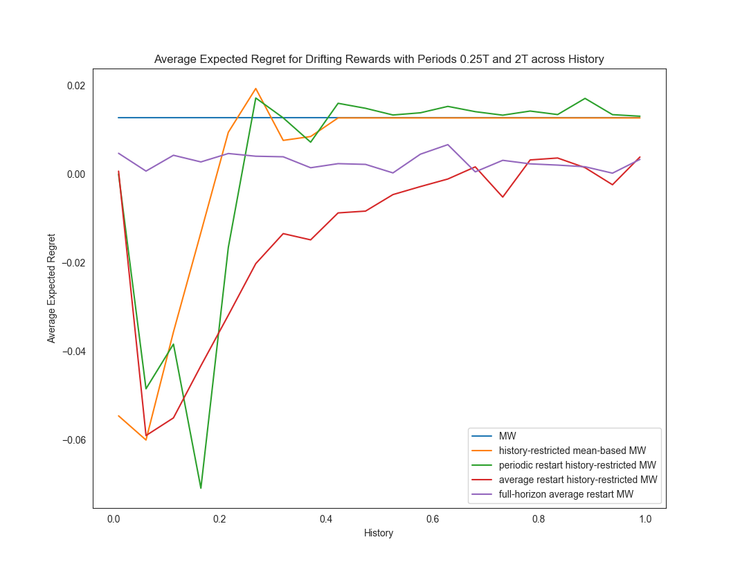
(f) $\varphi_{2}=2T$

Figure 20: We compare the average regret of our different algorithms across different choices of history for various drifting settings, with first arm having period $\varphi_{1}=T/4$ and second arm with period $\varphi_{2}$.

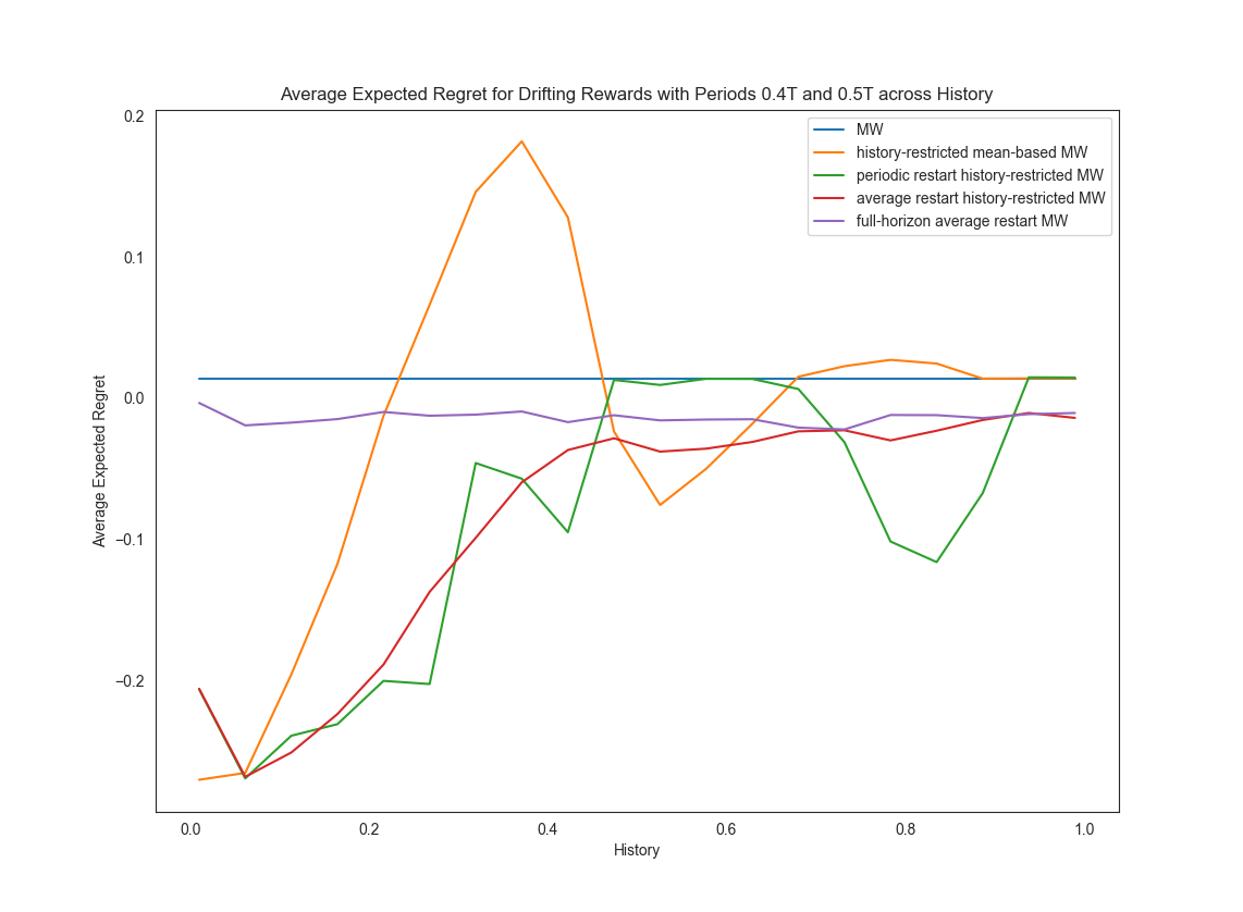
(a) $\varphi_{2}=T/2$

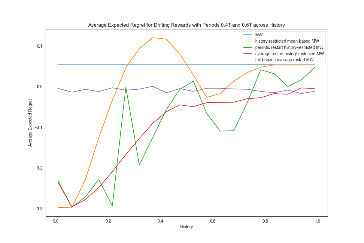
(b) $\varphi_{2}=3T/5$

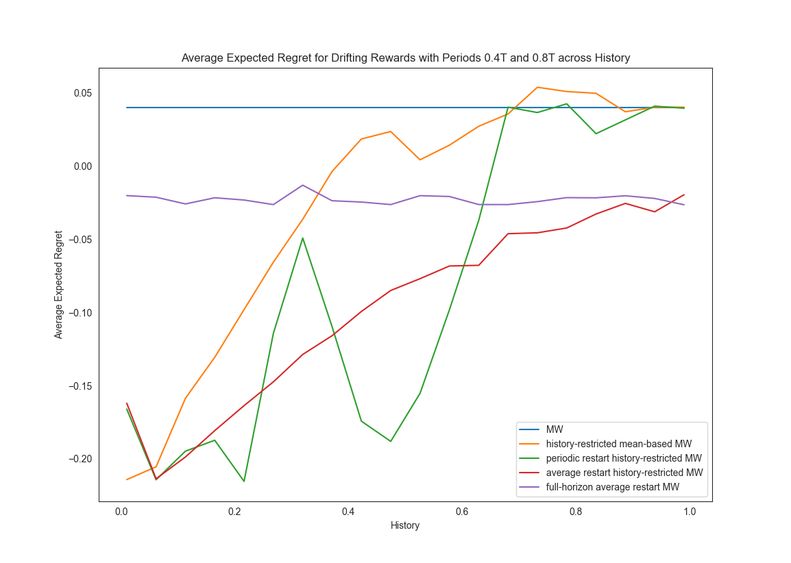
(c) $\varphi_{2}=4T/5$

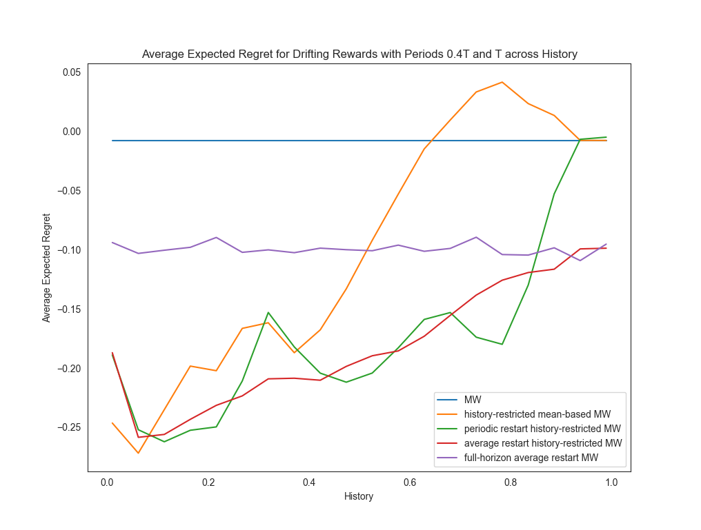
(d) $\varphi_{2}=T$

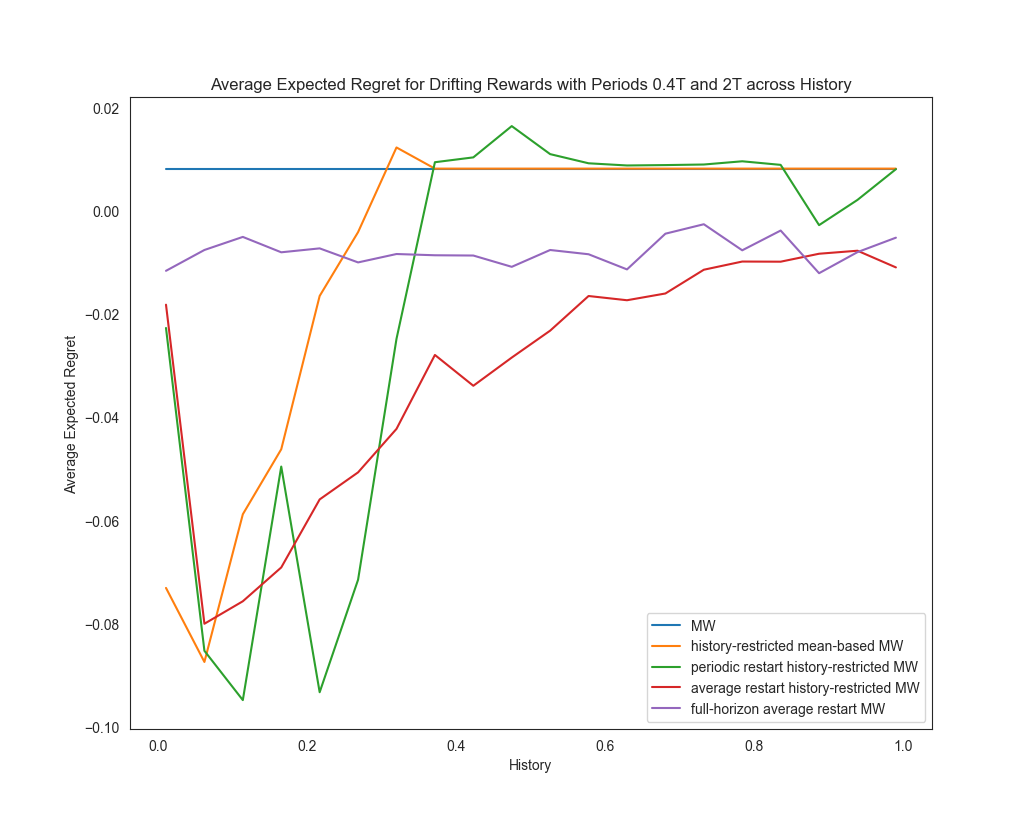
(e) $\varphi_{2}=2T$

Figure 21: We compare the average regret of our different algorithms across different choices of history for various drifting settings, with first arm having period $\varphi_{1}=2T/5$ and second arm with period $\varphi_{2}$.

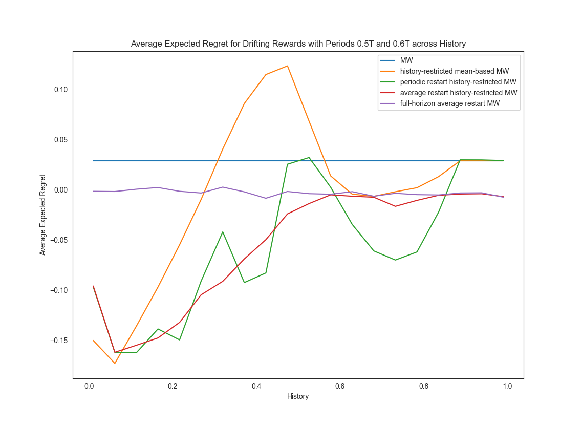
(a) $\varphi_{2}=3T/5$

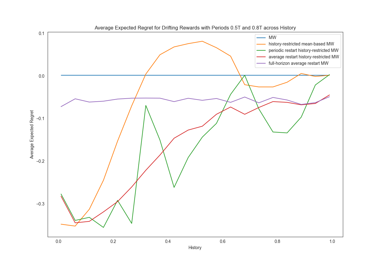
(b) $\varphi_{2}=4T/5$

(c) $\varphi_{2}=T$

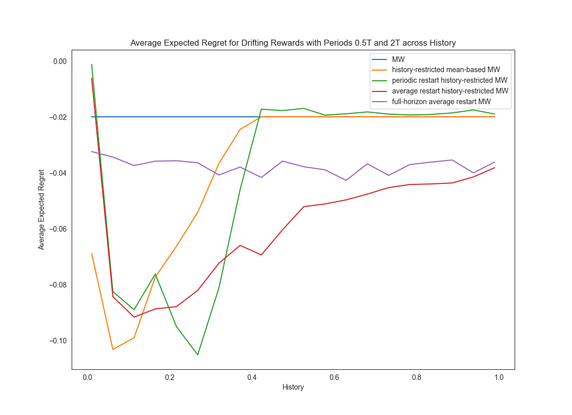
(d) $\varphi_{2}=2T$

Figure 22: We compare the average regret of our different algorithms across different choices of history for various drifting settings, with first arm having period $\varphi_{1}=T/2$ and second arm with period $\varphi_{2}$.

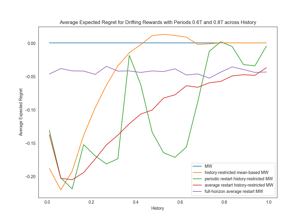
(a) $\varphi_{2}=4T/5$

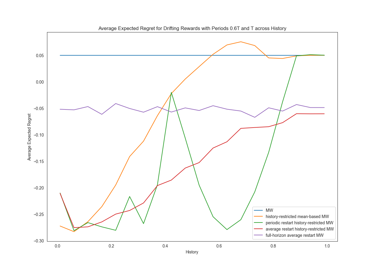
(b) $\varphi_{2}=T$

(c) $\varphi_{2}=2T$

Figure 23: We compare the average regret of our different algorithms across different choices of history for various drifting settings, with first arm having period $\varphi_{1}=3T/5$ and second arm with period $\varphi_{2}$.

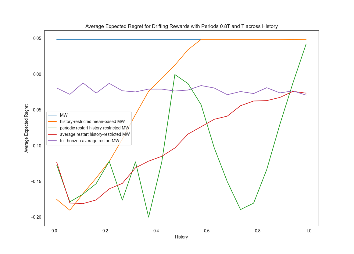
(a) $\varphi_{2}=T$

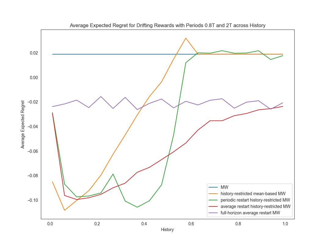
(b) $\varphi_{2}=2T$

Figure 24: We compare the average regret of our different algorithms across different choices of history for various drifting settings, with first arm having period $\varphi_{1}=4T/5$ and second arm with period $\varphi_{2}$.

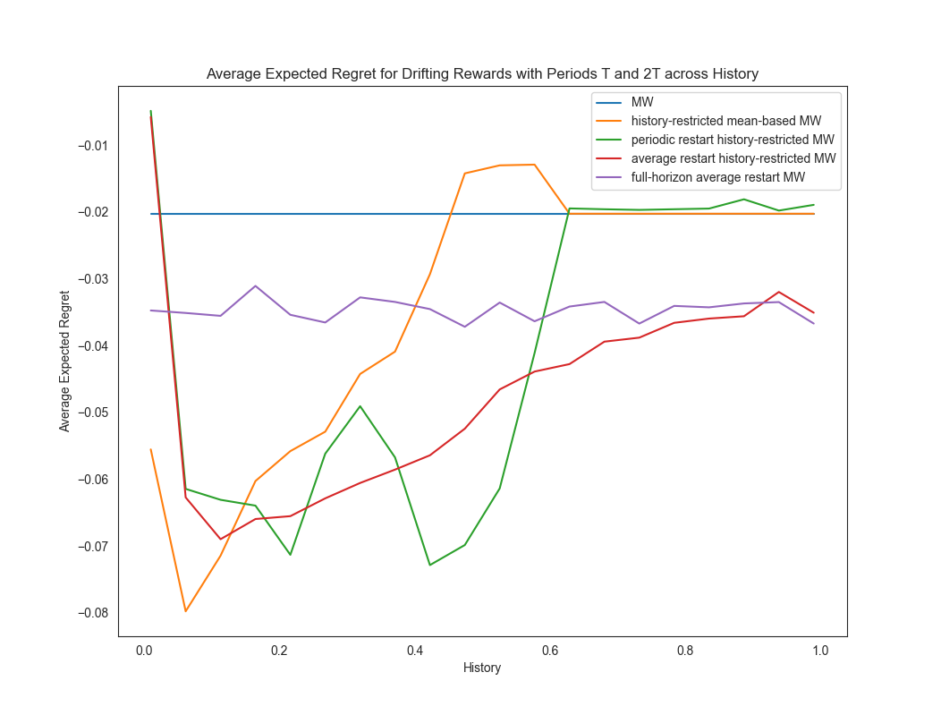
Figure 25: We compare the average regret of our different algorithms across different choices of history for a drifting setting where $\varphi_{1}=T,\varphi_{2}=2T$. It is particularly interesting that the average restart algorithmic paradigm improves over the others.

D.2 Heat Maps

Here we present heat map plots for four reward settings where the depth of the color red codifies the average regret across many choices of history parameter $M$ (we report $M$ as a fraction of $T$) and the number of rounds. We plot all history-restricted algorithms for each of the four settings.

Our takeaways are as follows:

1. Note the non-uniform impact of the history parameter – smaller histories to result in lower average regret in our chosen highly periodic settings.

2. The periodicity in the drifting rewards is exploitable by smaller history parameters.

3. The periodic restart algorithm is much less smooth in total regret performance as a function of the history parameter across the total regret trajectory as well, compared to the other two algorithms we consider.

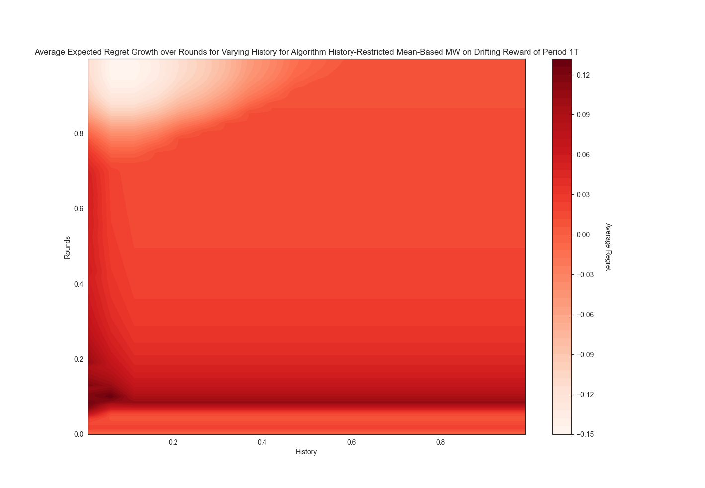
(a) Periodic Drifting Reward with $\varphi=T$.

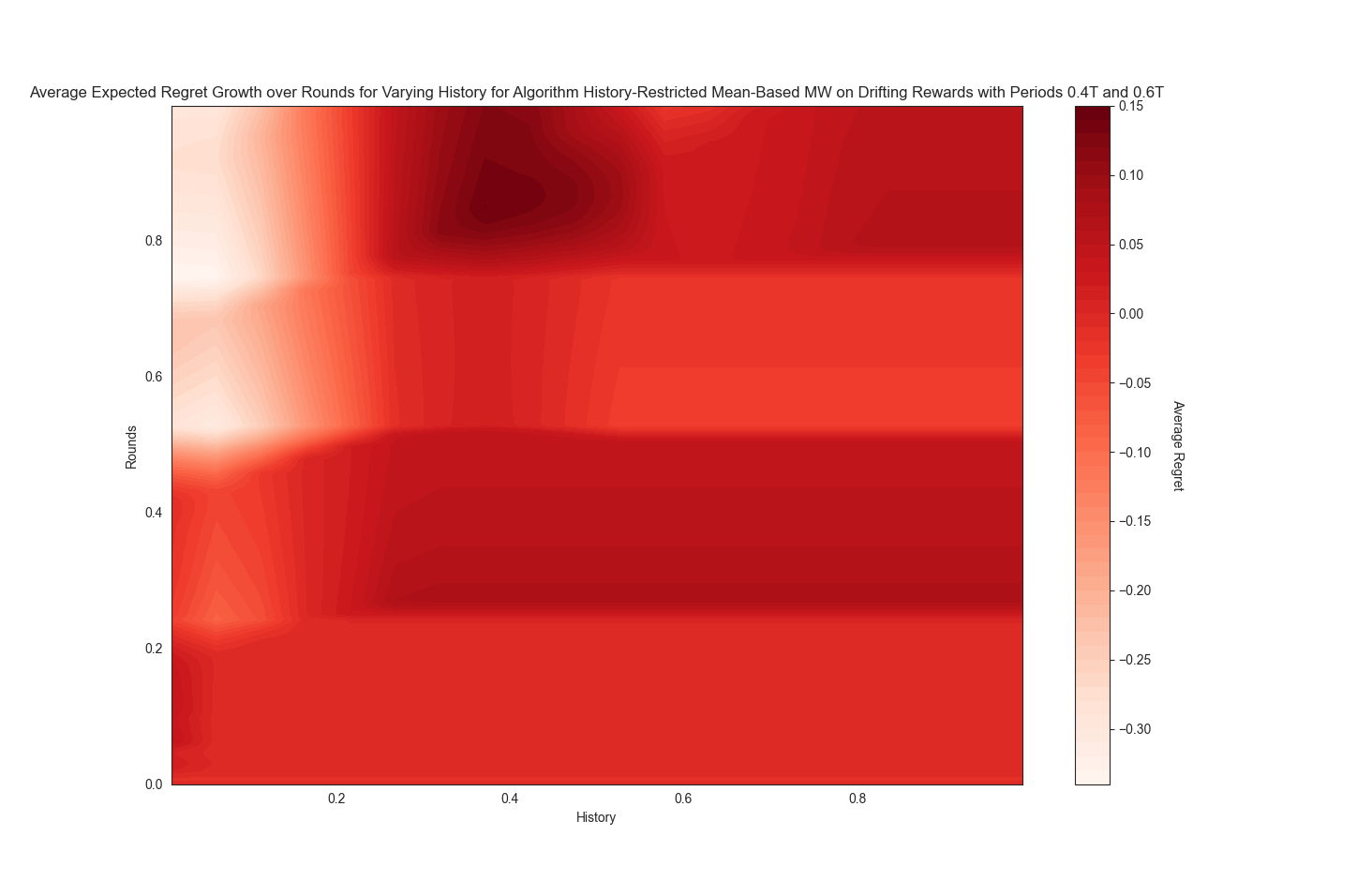
(b) Paired Periodic Drifting Reward with $\varphi_{1}=2T/5$ and $\varphi_{2}=3T/5$.

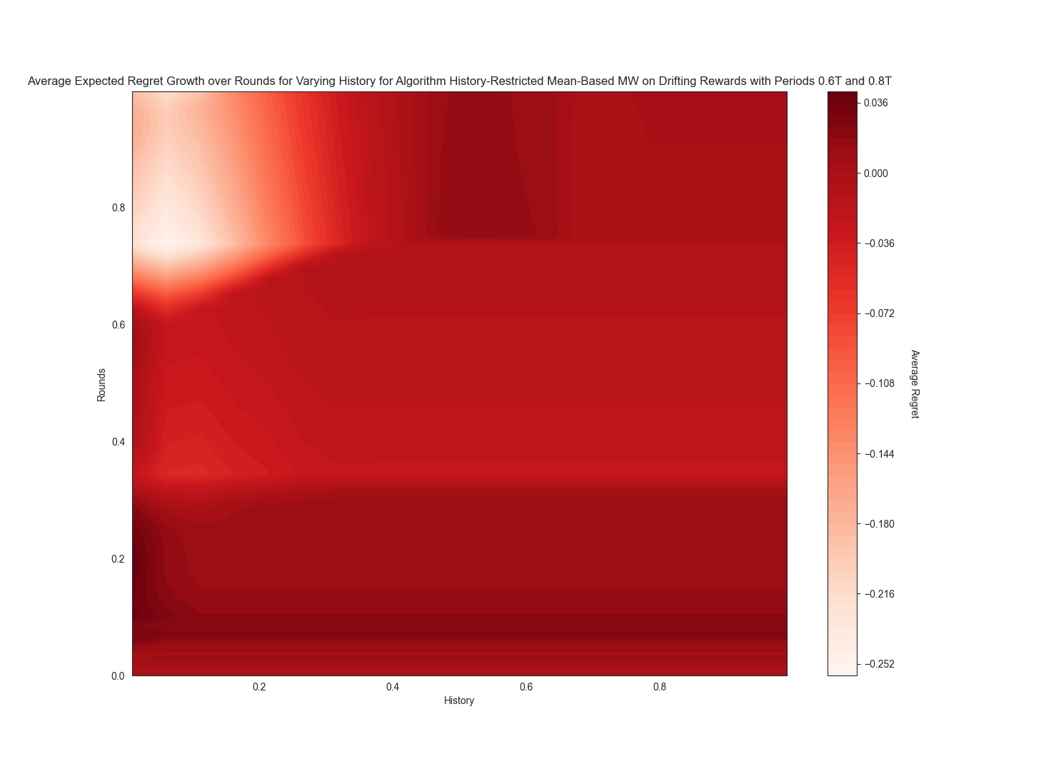
(c) Paired Periodic Drifting Reward with $\varphi_{1}=3T/5$ and $\varphi_{2}=4T/5$.

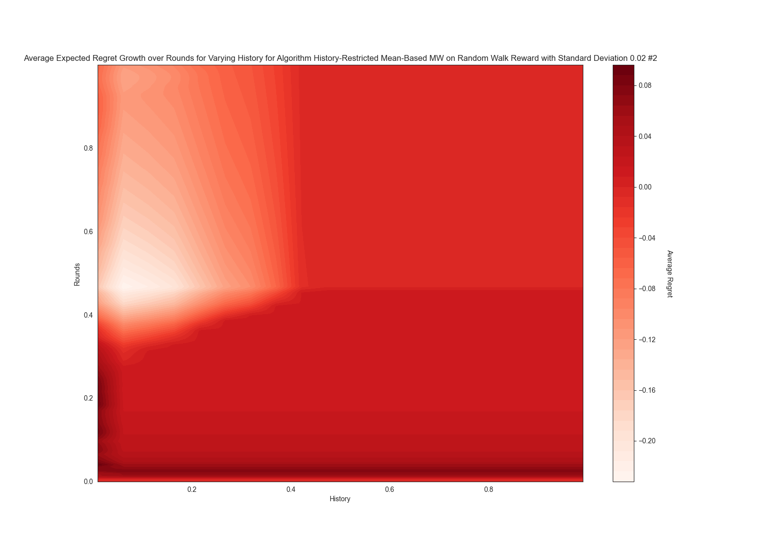
(d) Random Walk $\#2$ Reward with $\sigma=0.02$.

Figure 26: We compare the total regret evolution over time for the mean-based history restricted algorithm (Algorithm 4) across different choices of history for various reward settings.

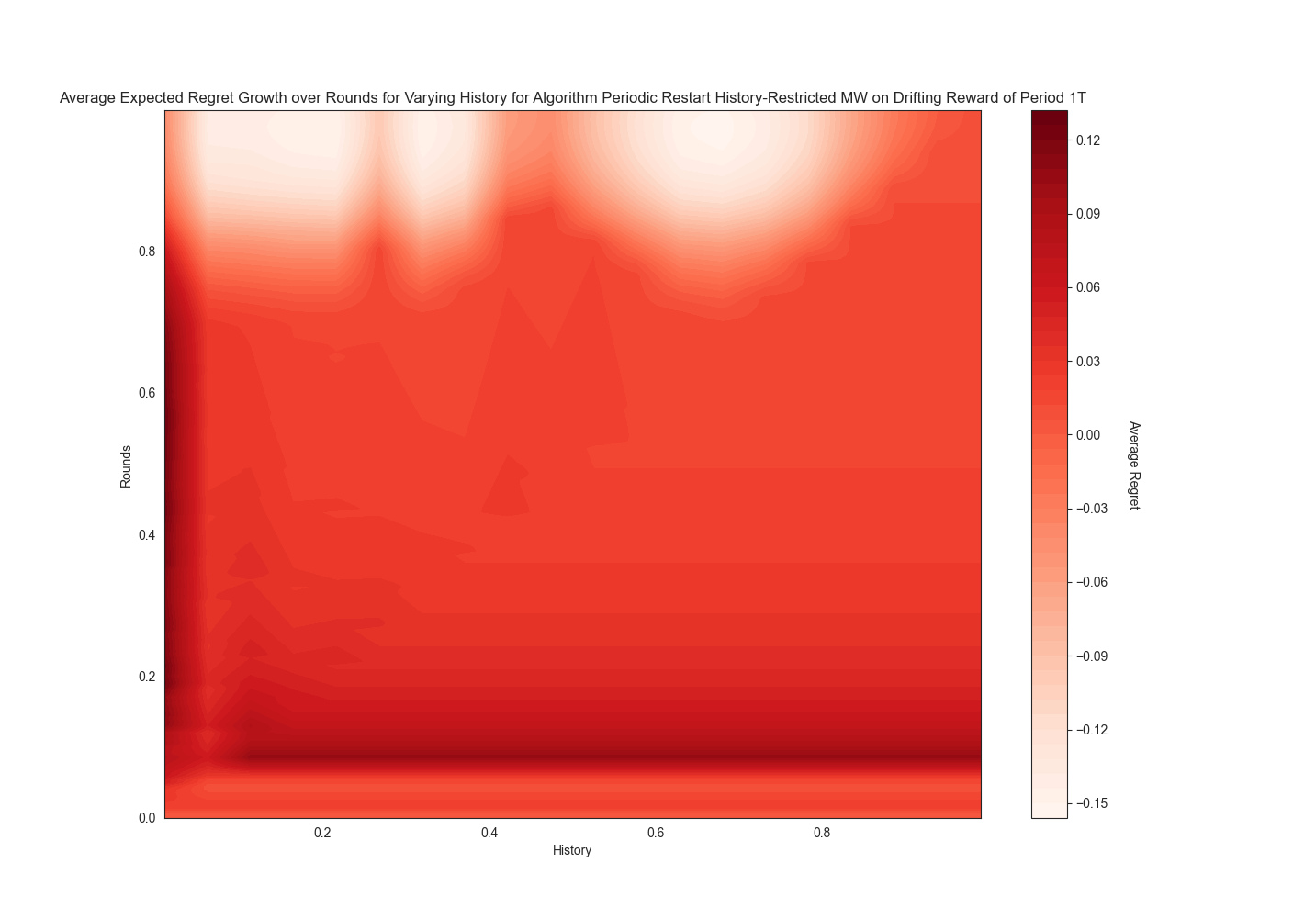
(a) Periodic Drifting Reward with $\varphi=T$.

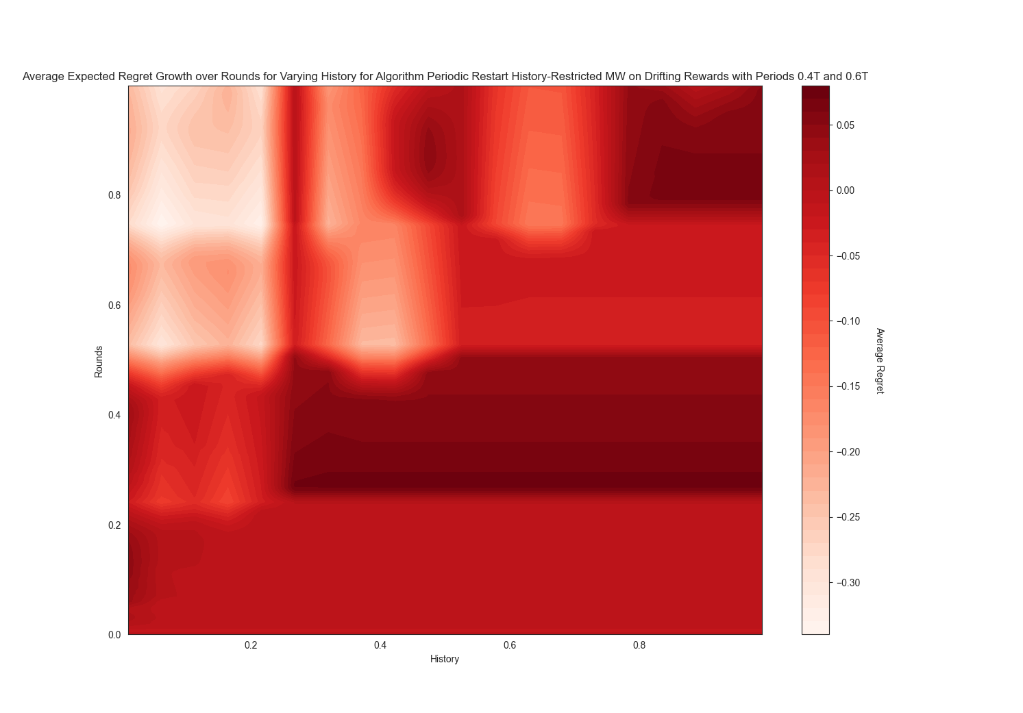
(b) Paired Periodic Drifting Reward with $\varphi_{1}=2T/5$ and $\varphi_{2}=3T/5$.

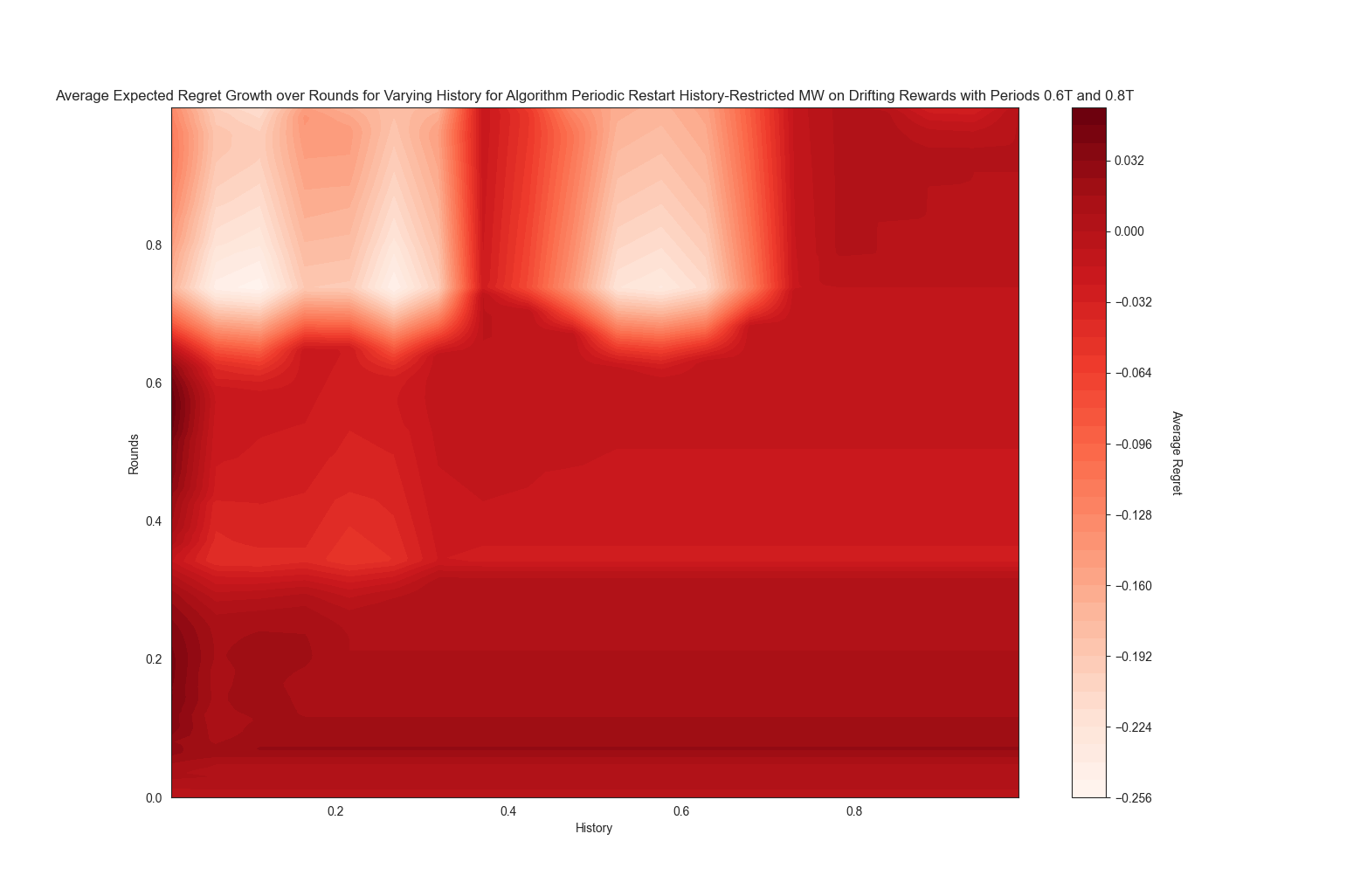
(c) Paired Periodic Drifting Reward with $\varphi_{1}=3T/5$ and $\varphi_{2}=4T/5$.

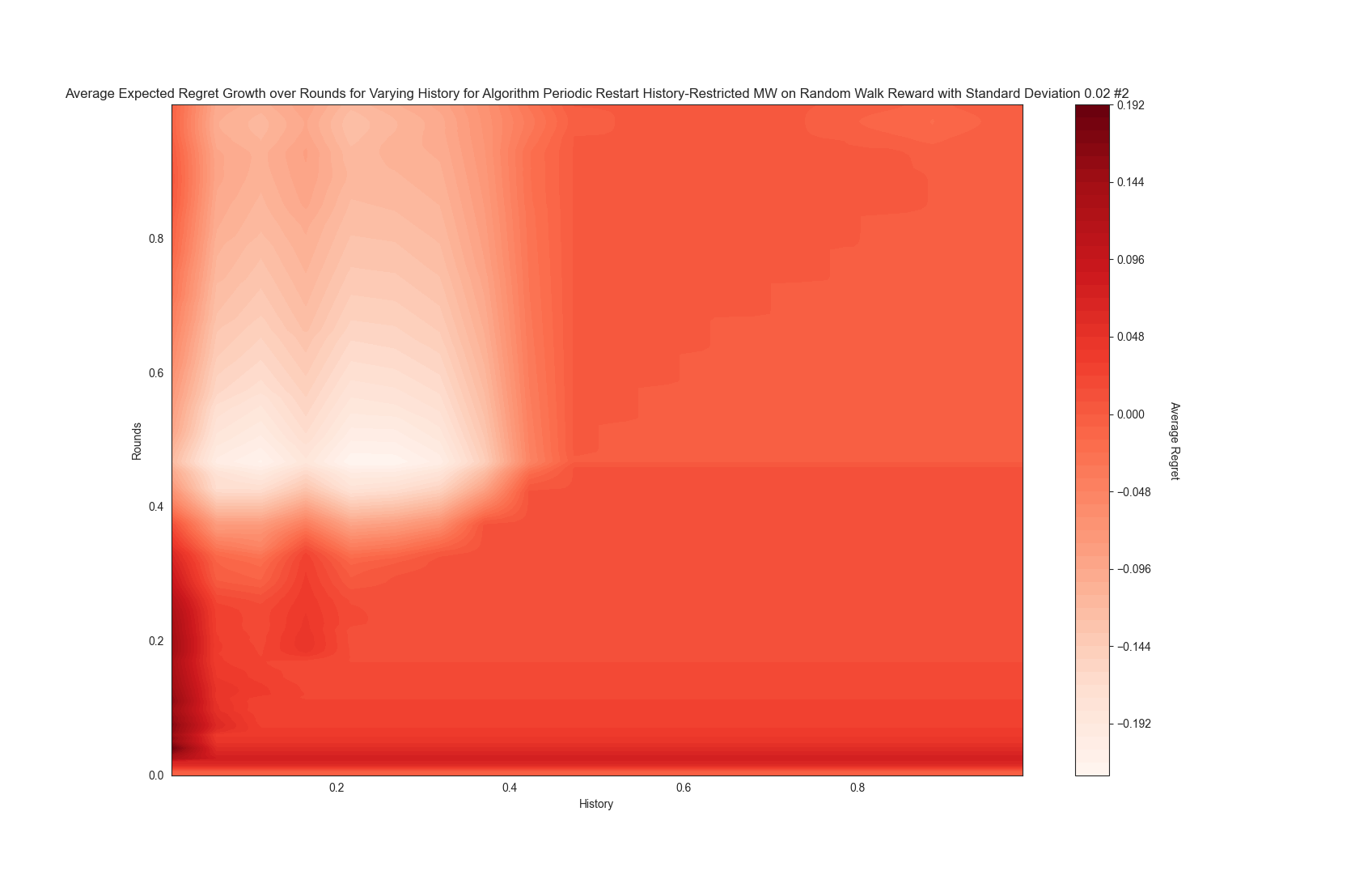
(d) Random Walk $\#2$ Reward with $\sigma=0.02$.

Figure 27: We compare the total regret evolution over time for the periodic restart algorithm (Algorithm 1) across different choices of history for various reward settings.

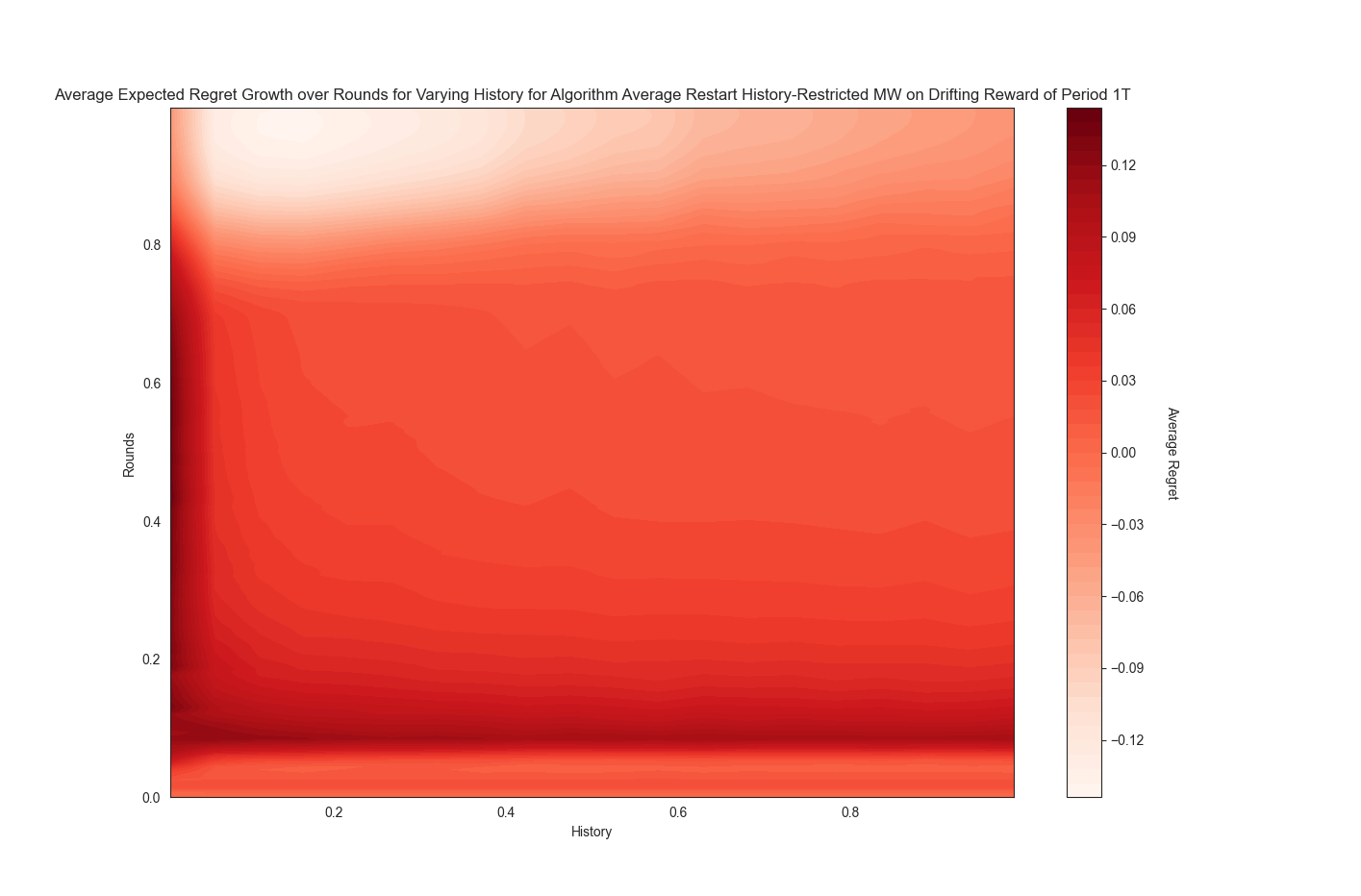
(a) Periodic Drifting Reward with $\varphi=T$.

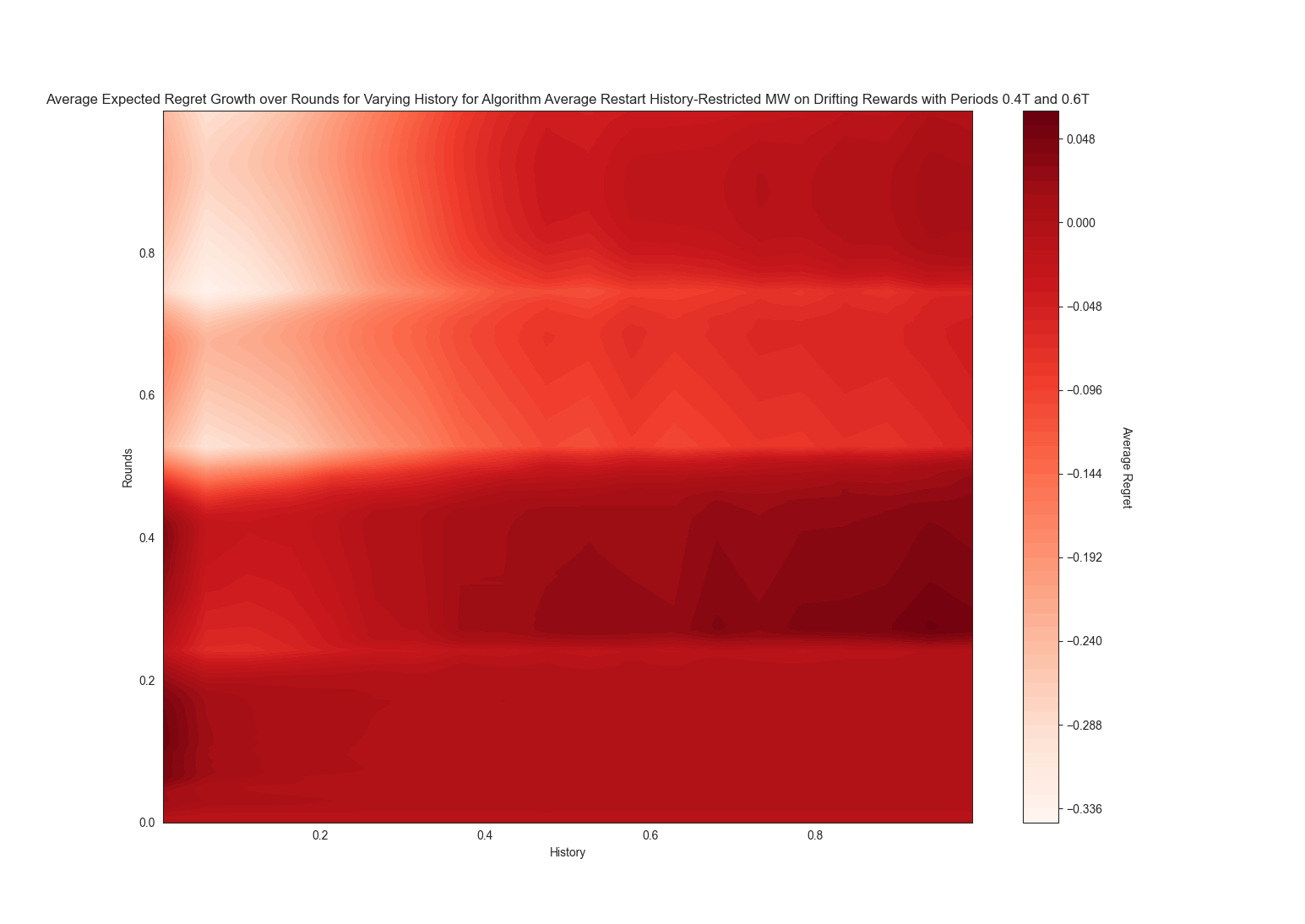
(b) Paired Periodic Drifting Reward with $\varphi_{1}=2T/5$ and $\varphi_{2}=3T/5$.

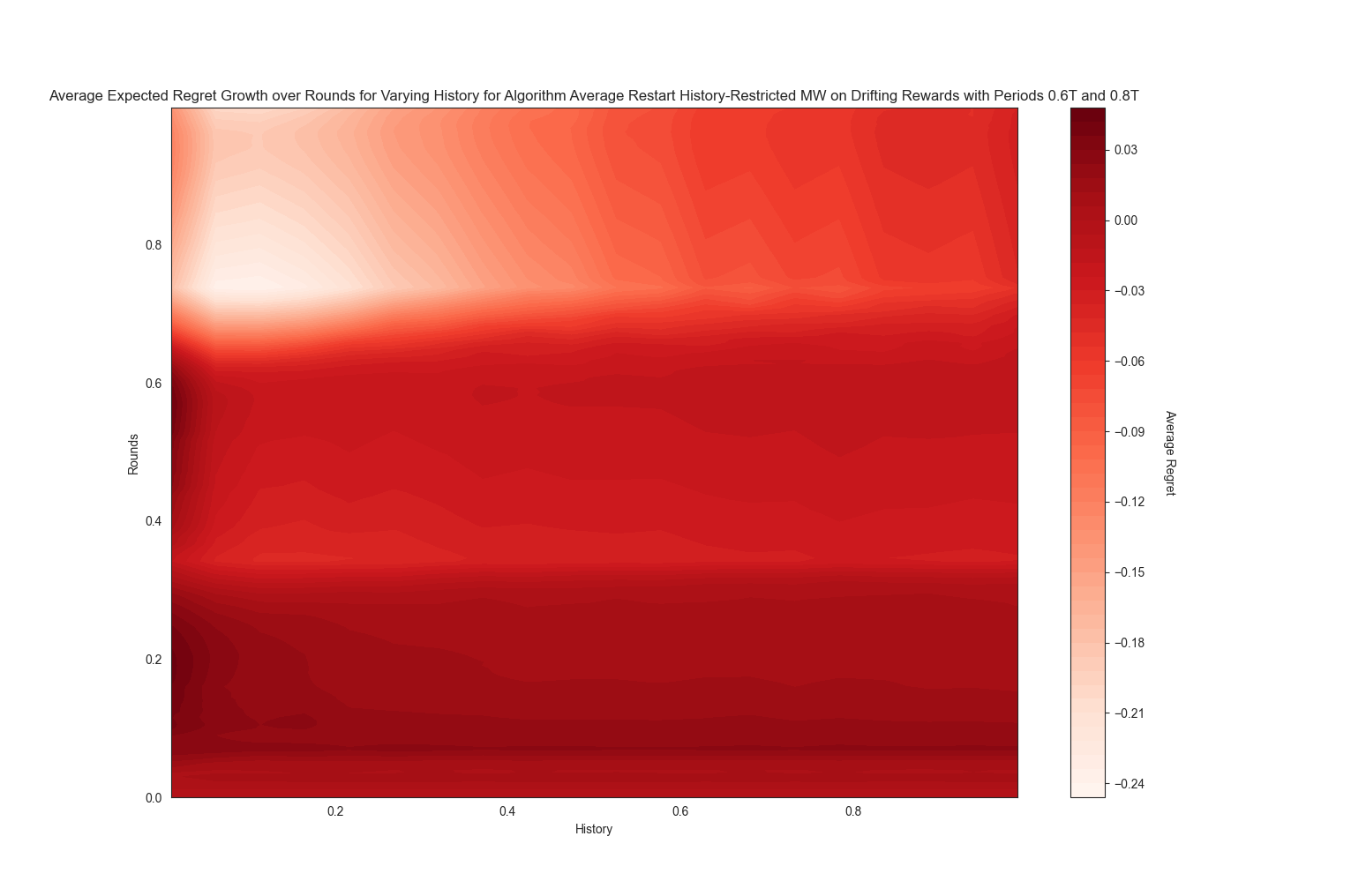
(c) Paired Periodic Drifting Reward with $\varphi_{1}=3T/5$ and $\varphi_{2}=4T/5$.

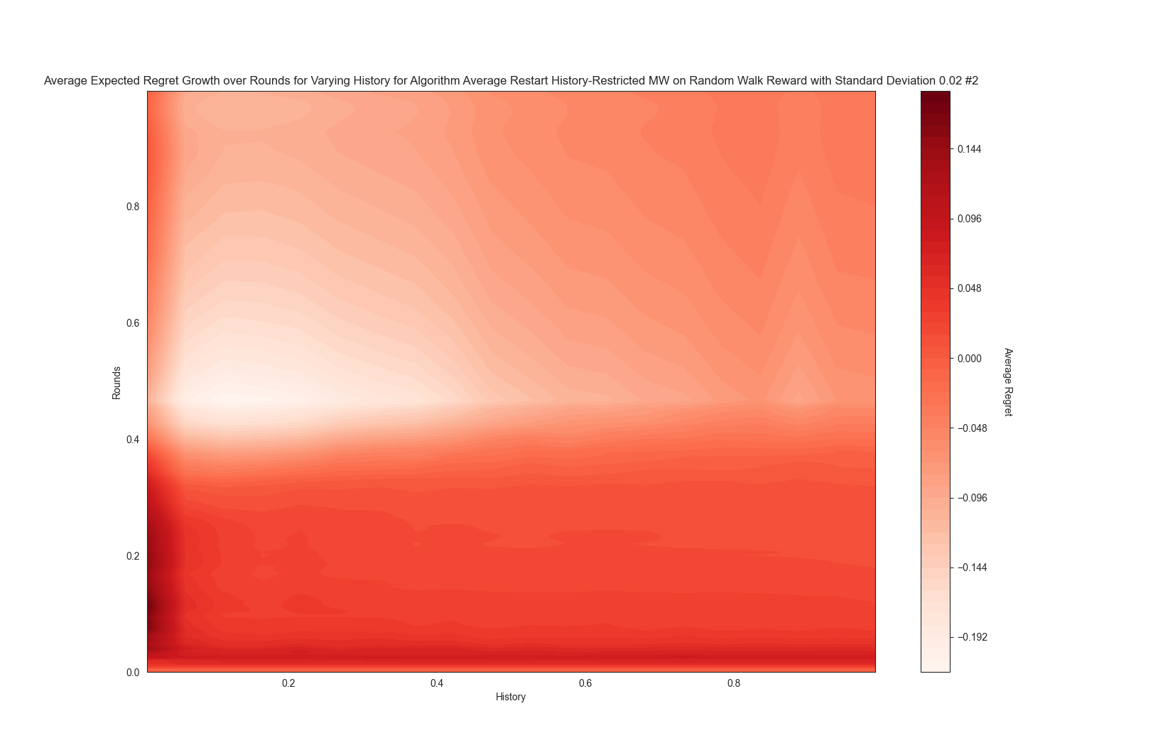
(d) Random Walk $\#2$ Reward with $\sigma=0.02$.

Figure 28: We compare the total regret evolution over time for the history-restricted average restart algorithm (Algorithm 2) across different choices of history for various reward settings.

References

- Arora et al. (2012) Sanjeev Arora, Elad Hazan, and Satyen Kale. The multiplicative weights update method: a meta-algorithm and applications. Theory of computing, 8(1):121–164, 2012.
- Blum and Mansour (2007a) Avrim Blum and Yishay Mansour. From external to internal regret. Journal of Machine Learning Research, 8(6), 2007a.
- Blum and Mansour (2007b) Avrim Blum and Yishay Mansour. Learning, regret minimization, and equilibria. 2007b.
- Braverman et al. (2018) Mark Braverman, Jieming Mao, Jon Schneider, and Matt Weinberg. Selling to a no-regret buyer. In Proceedings of the 2018 ACM Conference on Economics and Computation, pages 523–538, 2018.
- Cesa-Bianchi et al. (2007) Nicolo Cesa-Bianchi, Yishay Mansour, and Gilles Stoltz. Improved second-order bounds for prediction with expert advice. Machine Learning, 66(2):321–352, 2007.
- Chastain et al. (2013) Erick Chastain, Adi Livnat, Christos Papadimitriou, and Umesh Vazirani. Multiplicative updates in coordination games and the theory of evolution. In Proceedings of the 4th conference on Innovations in Theoretical Computer Science, pages 57–58, 2013.
- De Rooij et al. (2014) Steven De Rooij, Tim Van Erven, Peter D Grünwald, and Wouter M Koolen. Follow the leader if you can, hedge if you must. The Journal of Machine Learning Research, 15(1):1281–1316, 2014.
- Erven et al. (2011) Tim Erven, Wouter M Koolen, Steven Rooij, and Peter Grünwald. Adaptive hedge. Advances in Neural Information Processing Systems, 24, 2011.
- Ginart et al. (2019) Antonio Ginart, Melody Guan, Gregory Valiant, and James Y Zou. Making ai forget you: Data deletion in machine learning. Advances in Neural Information Processing Systems, 32, 2019.
- Hazan and Kale (2010) Elad Hazan and Satyen Kale. Extracting certainty from uncertainty: Regret bounded by variation in costs. Machine learning, 80(2):165–188, 2010.
- Huyen (2022) Chip Huyen. Data distribution shifts and monitoring, Feb 2022. URL https://huyenchip.com/.
- Kairouz et al. (2021) Peter Kairouz, H Brendan McMahan, Brendan Avent, Aurélien Bellet, Mehdi Bennis, Arjun Nitin Bhagoji, Kallista Bonawitz, Zachary Charles, Graham Cormode, Rachel Cummings, et al. Advances and open problems in federated learning. Foundations and Trends® in Machine Learning, 14(1–2):1–210, 2021.
- Koolen et al. (2016) Wouter M Koolen, Peter Grünwald, and Tim Van Erven. Combining adversarial guarantees and stochastic fast rates in online learning. Advances in Neural Information Processing Systems, 29, 2016.
- Lécuyer et al. (2019) Mathias Lécuyer, Riley Spahn, Kiran Vodrahalli, Roxana Geambasu, and Daniel Hsu. Privacy accounting and quality control in the sage differentially private ml platform. In Proceedings of the 27th ACM Symposium on Operating Systems Principles, pages 181–195, 2019.
- Mourtada and Gaïffas (2019) Jaouad Mourtada and Stéphane Gaïffas. On the optimality of the hedge algorithm in the stochastic regime. Journal of Machine Learning Research, 20:1–28, 2019.
- Nekipelov et al. (2015) Denis Nekipelov, Vasilis Syrgkanis, and Eva Tardos. Econometrics for learning agents. In Proceedings of the sixteenth acm conference on economics and computation, pages 1–18, 2015.
- Rabanser et al. (2019) Stephan Rabanser, Stephan Günnemann, and Zachary Lipton. Failing loudly: An empirical study of methods for detecting dataset shift. Advances in Neural Information Processing Systems, 32, 2019.
- Roughgarden (2016) Tim Roughgarden. Online learning and the multiplicative weights algorithm, February 2016.
- Sugiyama and Kawanabe (2012) Masashi Sugiyama and Motoaki Kawanabe. Machine learning in non-stationary environments: Introduction to covariate shift adaptation. MIT press, 2012.
- Voigt and Von dem Bussche (2017) Paul Voigt and Axel Von dem Bussche. The eu general data protection regulation (gdpr). A Practical Guide, 1st Ed., Cham: Springer International Publishing, 10(3152676):10–5555, 2017.
- Wiles et al. (2021) Olivia Wiles, Sven Gowal, Florian Stimberg, Sylvestre Alvise-Rebuffi, Ira Ktena, Taylan Cemgil, et al. A fine-grained analysis on distribution shift. arXiv preprint arXiv:2110.11328, 2021.
- Wu (2021) Yifan Wu. Learning to Predict and Make Decisions under Distribution Shift. PhD thesis, Carnegie Mellon University, 2021.